Stochastic Modelling of
Symmetric Positive Definite Material Tensors
Stochastic Modelling of
Symmetric Positive Definite Material Tensors
Abstract
Spatial symmetries and invariances play an important role in the behaviour of materials and should be respected in the description and modelling of material properties. The focus here is the class of physically symmetric and positive definite tensors, as they appear often in the description of materials, and one wants to be able to prescribe certain classes of spatial symmetries and invariances for each member of the whole ensemble, while at the same time demanding that the mean or expected value of the ensemble be subject to a possibly ‘higher’ spatial invariance class. We formulate a modelling framework which not only respects these two requirements—positive definiteness and invariance—but also allows a fine control over orientation on one hand, and strength / size on the other. As the set of positive definite tensors is not a linear space, but rather an open convex cone in the linear space of physically symmetric tensors, we consider it advantageous to widen the notion of mean to the so-called Fréchet mean on a metric space, which is based on distance measures or metrics between positive definite tensors other than the usual Euclidean one. It is shown how the random ensemble can be modelled and generated, independently in its scaling and orientational or directional aspects, with a Lie algebra representation via a memoryless transformation. The parameters which describe the elements in this Lie algebra are then to be considered as random fields on the domain of interest. As an example, a 2D and a 3D model of steady-state heat conduction in a human proximal femur, a bone with high material anisotropy, is modelled with a random thermal conductivity tensor, and the numerical results show the distinct impact of incorporating into the constitutive model different material uncertainties—scaling, orientation, and prescribed material symmetry—on the desired quantities of interest.
Keywords:
stochastic material modelling, tensor-valued random variable, anisotropy,
spatial symmetries of ensemble and mean, Fréchet mean, Lie algebra representation,
directional and scaling uncertainty, human proximal femur, uncertainty quantification
1 Introduction
Heterogeneous materials and their statistical description are of great interest in many fields. The properties of such materials often vary considerably on the spatial scales of interest, and additionally in many cases the material properties are only described statistically, reflecting some underlying uncertainty as to the exact values. This leads to the idea of a stochastic/random representation of these properties. The material properties are naturally collected in tensor quantities, and these tensors are often of even order and physically symmetric—in elasticity this is often termed the major symmetry. Furthermore, when these tensorial properties appear in the definitions of stored energy or entropy production of stable systems, they are additionally positive definite. It is this class of even-order physically symmetric and positive definite (SPD) tensors which we are interested in describing. Well known examples of such tensors are the second-order tensors describing diffusion phenomena, mapping the gradient of some quantity to the flux of some related quantity, e.g. the thermal conductivity tensor mapping temperature gradients to fluxes of thermal energy. An example of a fourth-order tensor is the elasticity tensor of a linearly elastic material, which maps the strain tensor to the stress tensor. Any even-order tensor may be viewed as a linear mapping on the space of tensors of half the order by contracting over half the indices. By choosing a basis in the space of tensors of half the order, each such even-order tensor can hence be represented by a matrix; so the class we are interested in can thus be represented by SPD matrices. We shall switch to this matrix representation whenever it is convenient to do so.
Even though frequently the exact values of the tensorial entries may not be known, some properties resulting from general principles often are known; namely, often it is known what kind of symmetries or invariances are to be expected [87, 10, 63]. These invariances—we prefer the term invariance over symmetry here to avoid confusion with the afore mentioned physical symmetry, resp. the symmetry of the tensor as a linear mapping—under the operation of some symmetry group are well known, and here we concentrate on spatial point operations such as those defining isotropy. These symmetry groups are represented as linear transformation groups on the relevant space of even order tensors, or, equivalently, on the space of representing symmetric matrices mentioned above. Such transformation groups then define invariant subspaces which represent the tensors with the given invariance property. As the number of such point groups is larger in the case of fourth-order spatial tensors (e.g. [11, 8, 10]) than in the case of second-order spatial tensors [68], in our explicit treatment here we shall confine ourselves to second-order spatial tensors for the sake of simplicity and clarity. But the general idea applies to any even-order SPD tensor field.
So, after a choice of bases, what will be considered here are random SPD matrices, where certain invariances are known for the whole population, as well as for the mean. There is already quite a bit of previous work in this field, drawing on several sources, which will be reviewed only very cursory and briefly here. Random SPD matrices (e.g. [48]) arise in a number of fields, e.g. [96, 99, 47, 36], to name just some.
Each SPD matrix can be spectrally decomposed with positive eigenvalues and orthogonal eigenvectors. This separates size / strength aspects as encoded in the eigenvalues, and orientation as encoded in the eigenvectors. We see these two items as vital information about how the tensor / matrix acts, and we shall base our treatment on this fundamental decomposition. On the other hand, for the purpose of modelling or representing a tensor, the most comfortable and desirable is to find a representation on a linear space. It is one of the aims to show here how this may be achieved for the spectral decomposition. Geometrically speaking, the positive definite symmetric even-order tensors resp. SPD matrices are an open convex cone in the vector space of symmetric even-order tensors resp. symmetric matrices, and are thus a differentiable manifold, but not a vector space. The spectral decomposition with positive eigenvalues represents this cone, and it will be shown that this decomposition is connected to another differentiable manifold, which is even a Lie group—a manifold with a differentiable group structure. This is one of the uses of group theory here, and in the actual numerical modelling it just boils down to the use of the matrix exponential.
Differentiable manifolds can be represented—mostly only locally—on their tangent spaces. The analysis of manifolds is typically facilitated if they can be adorned with a Riemannian structure [90, 105, 107], and even more so if the manifold carries the structure of a Lie group, as then everything can be played down to the tangent space at the neutral element, i.e. the associated Lie algebra. The Lie algebra is mapped to the Lie group via the exponential map. Unfortunately, the manifold of SPD matrices is not a Lie group under normal matrix multiplication, although it is possible [3] to give the SPD manifold a new commutative or Abelian multiplicative group structure, which coincides with matrix multiplication on commuting matrices.
The second use of group theory is in the material symmetry induced group reduction [26] —introducing as many zeros in the tensor as possible through spatial rotations, or, equivalently, through reflections [10]. This well-known subject defines the different symmetry classes [10, 68]. For second-order spatial tensors this spatial group reduction completely determines the eigenvector transformation of the associated SPD matrix into classes defined by the number of degenerate or coinciding eigenvalues, whereas for e.g. for fourth-order tensors there is an iso-spectral sub-group in the relevant Lie group of orthogonal transformations, cf. e.g. [65, 66, 67, 68], which determines the eigen-strain distribution in the relevant elasticity class [87, 11, 13, 63, 8]. This is one more reason to confine ourselves here initially to second-order spatial tensors for the sake of brevity and simplicity of exposition, the corresponding more involved results for fourth-order spatial tensors (i.e. elasticity tensors) will be published elsewhere.
The spectral decomposition of a random SPD matrix has thus two components, the SPD diagonal matrix of eigenvalues and the orthogonal orientation matrix. In particular—as will be shown—this allows the independent control of the strength (or size or norm) of the tensor and of its directional properties. Both components may be random, and thus random orthogonal matrices have some relevance here as well [69, 54, 81, 36]. The manifold of SPD matrices may thus be modelled on the product of the two Lie groups [57, 38, 37] of orthogonal and of positive diagonal matrices, and ultimately on their Lie algebras—the vector space of skew-symmetric and the space of diagonal matrices. A somewhat similar approach is also explored in [36], where rotation angles are used for the representation of rotations, which is one way to parametrise the Lie algebra of skew matrices. Here the well-known Rodrigues formula will be used for that purpose.
The Euclidean structure on the direct sum of the Lie algebras just mentioned may then be mapped via the exponential map onto a product Riemannian structure on the product manifold of the two Lie groups which represents the SPD matrices. Such a Riemannian structure on a manifold as just alluded to allows one to define the length of paths, and thus shortest paths resp. geodesics, and hence to measure distances on the manifold. As the variational definition of mean, resp. average, or expectation—we will use these terms interchangeably—depends on the distance measure (e.g. [85, 40], cf. also Section 2), this leads to the question as to what is an adequate definition of the mean for SPD tensors. The usual arithmetic mean is wedded to a flat (vector-)space and a Euclidean distance, as is well known and will be explained in more detail later in Section 2.3. On a metric space the mean of two points is the point half-way along the shortest path between them. This generalisation is known as the Fréchet mean. This connection between the mean (and variance to be defined later) and a distance metric may be used to switch the discussion of what is desired from the mean to the underlying distance metric, as on a non-flat manifold the Euclidean metric of the ambient space is not advantageous. For example on the Lie group of orthogonal matrices it is completely common to use such a Riemannian metric [69, 54, 81].
On the manifold of SPD matrices the usual Euclidean metric of the ambient space of symmetric matrices is derived from the Frobenius resp. Hilbert-Schmidt inner product and norm. It has long been recognised that this metric has some undesirable properties [90, 1, 83, 2, 3, 22, 23, 31, 27], in particular the so-called swelling, fattening, and shrinking effects in interpolation resp. averaging [96, 57, 97, 38, 37]. This refers to the ellipsoid representing the SPD matrix, and is connected to the non-monotonic interpolation of the eigenvalues or some of their functions (e.g. the determinant) along Euclidean geodesics, i.e. straight lines. In the context of stochastic material modelling this means a loss of anisotropy for the whole ensemble, which may be undesirable in some situations. In the literature just cited, there is an intensive discussion—particularly coming from the medical field of diffusion tensor imaging, where these undesirable effects are not acceptable—on how to make the SPD tensors into a Riemannian manifold with different metrics [91]. From this one obtains variatonally the Fréchet or Karcher mean—the generalisation of the arithmetic resp. Euclidean mean to general metric spaces [85, 40, 39]. This is an area of active research [105, 106, 107], the ‘best’ metric and mean seem to be application dependent, and here we shall formulate some desiderata for a metric—and thus mean—for SPD tensors of material properties, and propose one which in our view is most suited for this kind of field. Subsequently, we use this proposed Fréchet mean, and it agrees nicely with the modelling in terms of a product Lie group, see also [56].
As to the modelling of random tensor fields with given invariance properties, the culmination of a long series of works [66, 88, 65, 64, 67] is reported in [68], which looks at stochastically homogeneous and isotropic random tensor fields of any order in a three dimensional domain. The results reported there allow a fine control about what invariance the mean of such a tensor field has, and what kind of invariance may be required of each realisation. Using the spectral theorem for the covariance of such homogeneous and isotropic fields, as well as the representation theory of the appropriate groups, here one may find the spectral resolution of the covariance function and from it a Karhunen-Loève like representation (e.g. [76]) of the random tensor field with the desired invariance properties. In these deliberations, no special attention is payed to the topic of positive definiteness, as the methods used are purely vector space like linear combinations or generalisations such as series and integrals. And although the limiting expression may well represent a positive definite tensor, in practical computational situations these series and integrals have to be truncated resp. numerically approximated, and this step may lead to a numerical loss of positive definiteness.
A reduced non-parametric approach to generate random SPD matrices, which takes explicit account of the topic of positive definiteness, was presented in [99, 100]. Here an algebraic property, namely that positive elements in the algebra are squares of other elements in the algebra, is used to ascertain that each generated tensor field is indeed SPD. This approach to ensure positivity is also examined in [36]. Based on this, the generation of random elasticity tensors with specified invariance in the mean and fully anisotropic invariance in each realisation, resp. controlled elasticity class invariance with constant spatial orientation of the symmetry axes in each realisation, is shown in a series of papers [41, 42, 43, 44, 45, 46, 86, 102, 101].
Another example for a frequent approach to ensure the SPD property is to use the exponential function, resp. the logarithm in the opposite direction. This is employed in e.g. [45, 86, 57, 97, 38, 37], and it can even be combined with the previous squaring approach [45, 86, 36] to ensure compliance with a particular invariance class. This technique is used quite widely when describing measured diffusion and conductivity tensors, namely instead of addressing the SPD tensor itself, one focuses with the description on its logarithm. To obtain the tensor, one finally takes the exponential, thus ensuring positive definiteness. This approach can take advantage of the fact that the invariance classes are the same for a tensor and its exponential. We shall follow a similar path here and essentially use the exponential function to ensure positive definiteness numerically in each realisation.
The plan of the paper is as follows. In Section 2 we formulate the overall problem more precisely and spell out the desiderata for the modelling and generation of symmetric positive definite (SPD) matrices, as well as for the mean, based on requirements for the metric. The desiderata for the mean or expectation will be set forth in Section 2.3. As we shall use the spectral decomposition in Section 3 to separate orientation and strength / size, and an appropriate definition of mean and corresponding modelling approach, one has also to be able to generate random orthogonal transformations. In the end the SPD matrix at each point in the domain for each realisation will be a function of a few new numerical parameters, here the logarithms of the eigenvalues as well as a description for the orthogonal eigenvector matrix, which we shall base on the Rodrigues formula via the so called rotation vector.
It is these eigenvalue parameters as well as the rotation vector which vary randomly and in the domain, a similar approach as in [36], where the angles describing the eigenvectors are random fields. On this level, the step to spatially random fields is relatively simple, and one may borrow the idea formulated in [41, 42, 43, 44, 45, 46, 36], and regard the representation parameters as random fields without any positivity or invariance constraints. This then automatically produces random SPD tensor fields when played back via the spatially point-wise exponential map on the product Lie group, and from these to the SPD tensors.
As the spatial variation of the random tensor fields is well known from the corresponding correlation functions—no matter what kind of mean was used for the computation of the correlation function, this can be converted to a joint correlation function for the log eigenvalues and the rotation vector. Spatially homogeneous and invariant-wise isotropic tensor fields, which is the subject of [68], are a special case of this more general approach. As may be gleaned from this short overview, ensuring positive definiteness and the proper invariance at each point and realisation is a main concern, so we focus mainly on this part. Random fields of the parameters can then be generated through well known synthesis techniques connected to the Karhunen-Loève representation (e.g. [76]), or even more general representations with tight frames [62], where no nonlinear constraints like positivity have to be observed, yielding the SPD matrix through a memoryless transformation.
We also have an application in mind, which will be used in numerical examples to demonstrate the workings of the different modelling assumptions. This is the thermal conductivity of bones — a highly anisotropic material — which is important in some surgical procedures [79, 4]. It is described in Section 4. The results of the computations are shown in Sections 4.1 and 4.2, which then displays the effect on actual computational results of different modelling assumptions about the anisotropy. While Section 5 concludes, some additional material on distance metrics for symmetric positive definite matrices is collected in Appendix A.
2 Problem description
Let be a bounded domain in a -dimensional Euclidean space (here or ), such that the behaviour of a physical system in the domain is governed by an abstract equation
| (1) |
Here describes the state of the system lying in a Hilbert space (for the sake of simplicity), is a—possibly non-linear—operator modelling the physics of the system, and is some external influence (action/excitation/loading).
Furthermore, the coefficient is regarded as a material tensor which represents intrinsic physics-based properties of materials, such as thermal conductivity, magnetic permeability, chemical diffusivity, and similar [87, 63]. It is modelled as a tensor-valued field, at each point in the domain taking values in the open convex cone of real-valued second order positive-definite tensors:
| (2) |
As a simple example of such an equation, the reader may think of the well known thermal conduction equation — the example to be used in the numerical experiments:
| (3) |
plus some appropriate boundary conditions on . Here the system state is described by the temperature at each point , the ‘loading’ are thermal sinks and sources, and is the second order tensor field of thermal conductivities.
2.1 Stochastic model
Coming back to the general model Eq.(1), due to uncertainties in the exact value of , which may be due to a highly heterogeneous material, or simply a lack of knowledge about the exact value, we assume that a probabilistic model is adopted, so that it is modelled as a second-order tensor valued random field, i.e. a mapping
| (4) |
on a probability space , where represents the sample space containing all outcomes , is the -algebra of measurable subsets of , and is a probability measure. Similarly, one may assume the boundary or initial conditions, as well as external actions to be uncertain. However, this is secondary to the purpose of this paper and will not be covered further. To avoid unnecessary clutter in the notation the argument will be omitted, unless it is necessary for an understanding of the expressions. The same will often be true of the argument .
Evidently, this change transforms Eq.(1) to its stochastic counterpart, taking the form
| (5) |
in which is a stochastic response, due to the randomness in . Here we shall not be concerned on how this stochastic response may be computed (see e.g. [76]), but primarily on how to represent the symmetric positive definite (SPD) tensor .
2.2 Representation requirements
One important point in the description of material properties of are symmetries in the sense of invariance against certain transformations. It is well known that the collection of all such transformations form a group [87, 68], and here we shall only be concerned with so-called point groups. The representation of any such subgroup of the spatial orthogonal group of is fairly direct, and invariance here means that for all one has , a homogeneous linear constraint on .
The set of tensors which satisfy such an invariance is easily seen to form a subspace in (e.g. [10, 68]), the invariant subspace of the action of . Hence the distribution of the lives only on this subspace, or more precisely on , as there will be no realisations outside of it.
For the mean , which is an averaging operation, it is possible (e.g. [10, 68]) that it is invariant w.r.t. a larger group . This property of the mean possibly having a larger symmetry group is commonly envoked e.g. when considering random assemblages of anisotropic crystals [10]. As was noted already in Section 1, it is not all obvious which kind of mean to take here, as it depends on how is seen as a metric manifold with metric ; more about that will follow further below in Section 2.3 and in Appendix A. This implies that
as due to the -invariant subspace must be a subspace of the -invariant subspace . All this leads to the following requirements for the parametrisation of :
-
1.
Each has to be symmetric, i.e. .
-
2.
Even under numerical approximations like truncation of series resp. numerical quadrature, each realisation has to be SPD, i.e. for all .
-
3.
has to be invariant under some group of transformations , the invariance or symmetry class of each realisation.
-
4.
The appropriate mean has to be invariant under a possibly larger group of transformations , with , the invariance or symmetry class of the mean .
The first, third, and fourth item are not difficult to satisfy, as they are linear constraints in the vector space of all matrices, all one has to do is to pick an appropriate basis. The first item is almost trivial, and the second item is elaborated on in Section 3.1. The third and fourth point are discussed in Section 3.2, whereas the question of the mean in the fourth item will be addressed in the following Section 2.3.
2.3 Means for symmetric positive definite matrices
The second and third items on the above requirements list will be discussed in more detail later, but to discuss the fourth item, one has to first define the kind of mean or average resp. expected value one wants to use. As was already alluded to in Section 1, this is very much connected to the way in which distances on are measured. And computing a weighted mean between two items is actually a way of interpolating. The next few paragraphs are meant to illustrate and remind the reader of this connection.
It has been well known since antiquity that there are different ways to compute a mean or an average, one just has to look at the classical Pythagorean means. The arithmetic or Euclidean mean of a set of vectors —best known by almost anyone is the case —with standard Euclidean squared norm and corresponding Euclidean distance , is given by
| (6) |
which displays right away the variational characterisation of the mean by elementary calculus. The minimal value of the function is called the variance of the set . Observe that the terms in Eq.(6) are the squares of the Euclidean distances between and . One may also note that for one gets from Eq.(6) that is the half-way interpolation on the ‘shortest path’—the straight line—between and , which is an elementary example of the connection between averaging and interpolation.
The Eq.(6) is easily generalised to not necessarily equal (probability) weights , , instead of the constant , and vectors in any Euclidean vector space with inner product and corresponding norm, giving . Hereby it was assumed that—as is the case for an isotropic Euclidean distance—the gradient of the inner product is .
The generalisation of Eq.(6) corresponding to a general probability distribution of a -valued random variable would be
| (7) |
and again the minimum is the variance of the distribution .
In case the underlying set does not have a vector space structure but only that of a metric space, i.e. when only a distance metric is defined, or, like in our case, another distance than the Euclidean is to be used, one may define the so-called Fréchet mean or average attached to that metric [85, 91, 40, 39] through a variational characterisation similar to Eqs.(6) and (7), by replacing the Euclidean metric in those expressions by . Thus one may define the Fréchet-Karcher mean on such a metric space with a distance function which is at the same time a measure space with a general probability measure for an -valued random variable as
| (8) |
and again the variance is defined by the minimum value . If a unique minimiser exists, for general metric spaces this is called the Fréchet mean and variance, and for Riemannian manifolds a local minimiser of the variance functionals in Eq.(8) is also sometimes called the Karcher mean [85, 91, 40, 39].
These foregoing observations show the intimate connection between distance metric, mean or average and expectation, and interpolation. The properties of the Fréchet mean or average depend completely on the underlying metric, see Eqs.(6) and (8). Turning now to positive definite tensors , as mentioned already in Section 1, the Euclidean or Frobenius resp. Hilbert-Schmidt norm (cf. Eq.(49) in Appendix A) has long been recognised to result in some undesirable properties [90, 1, 83, 2, 3, 22, 23, 31], especially the swelling, fattening, and shrinking effects in interpolation resp. averaging [96, 57, 97, 38, 37, 27]. It is therefore of considerable interest to consider different metrics on [91, 85, 27]. In order not to distract the reader’s attention too much by reviewing different metrics used on , we relegate this material to Appendix A. Having chosen some distance metric with desirable properties on , one defines the -based Fréchet variance analogous to Eqs.(6) and (8):
| (9) |
From this one obtains the definition of the corresponding Fréchet or Karcher mean resp. expectation
| (10) |
Inserting this minimiser—if it exists—into the functional Eq.(9), one obtains the variance of the -valued random variable as the minimum value .
Let us collect here some, in our view desirable, properties of a possible metric for material tensors , which then may point to a certain kind of mean to use. As an extreme case one could argue that the mean should be such, that if used in Eq.(1), one obtains the mean of the stochastic solution of Eq.(5):
| (11) |
This is in fact the goal of homogenisation techniques, see e.g. [58, 51], but it is probably too much to require from a general kind of average, as it would depend on the model Eqs.(1) and (5) and thus be highly problem dependent. Hence we try and settle with some more general requirements based on invariance considerations. The invariance requirements for the metric translate immediately into invariance requirements for the corresponding Fréchet mean.
From the point of physical modelling, if appears in a constitutive model, there is typically an inverse formulation involving . This means that one normally knows as much about the distribution of as about the distribution of , as the set is stable under inversion. So one property of a desired metric on would be invariance under inversion. Changing physical units would correspond to a scaling by a positive factor, so the desired metric should be invariant under scaling. And as a change of the coordinate frame by an orthogonal transformation changes the constitutive tensor to , one would like the desired metric to be invariant under such transformations in order to respect the principle of frame indifference. Collecting everything, the desiderata for a metric , and hence for a Fréchet mean based on it via Eq.(10), then are to satisfy for all , , and all :
-
•
invariance under inversion: ;
-
•
invariance under scaling: ;
-
•
invariance under frame transformations: .
By choosing a metric on which satisfies those requirements, the Fréchet-Karcher mean based on that metric will automatically inherit all those properties, as can be easily gleaned from the very definition above in Eqs.(9) and (10).
The usual Frobenius resp. Euclidean distance which leads to the normal arithmetic mean Eq.(7) satisfies the last requirement, but not the first two. Additionally, the swelling, fattening, and shrinking effects that result from the straight line interpolation or averaging in the vector space of two elements of are highly undesirable [2, 96, 57, 97, 38, 37, 27]. Any Fréchet-Karcher mean based on a distance function which exhibits these undesirable effects in interpolation would also exhibit these effects in the averaging procedure, i.e. the thus defined mean would be more swollen, fatter, or shrunk than the population it is derived from. This short consideration shows that the normal arithmetic or Euclidean mean based on the Frobenius distance (Eq.(50) in Appendix A) is not ideal for SPD material tensors.
What comes out of from the more detailed considerations in Appendix A regarding possible metrics on , is that all the other distance metrics considered there, namely the geometric or affine-invariant distance (Eq.(51) in Appendix A), the logarithmic or log-Euclidean distance (Eq.(54) in Appendix A), and the scaling-rotation distance—which we will often refer to as just the scaling distance— (Eq.(58) in Appendix A), and which in turn is based on the product Lie group distance (Eq.(56) in Appendix A), all satisfy all of the above three requirements. This means that for a choice between them additional considerations are necessary. These are how to ensure the requirement listed above in Section 2.2, namely how to ensure positive definiteness through an appropriate representation, and at the same time ensure the symmetry class of the corresponding mean and each single realisation. One may note that we have defined as an open convex cone in , which means that all elements are positive definite. Thus any average or mean, which in a vector space is located in the convex hull of the support of the probability distribution will also be positive definite. In our approach in Section 3 this is ensured by modelling the logarithms of the eigenvalues. A slightly different situation may arise when [22, 23] experimental or measured covariance matrices are averaged. Such matrices may be rank deficient, i.e. singular, or symmetric positive but not definite, and thus geometrically on the boundary of the convex cone of positive definite matrices. In this case the arithmetic mean may also be singular and thus not positive definite, but the other Fréchet means may more readily give an average in the interior of the cone, and hence a positive definite mean.
In the following Section 3, where the modelling of SPD tensors based on the chosen representation is described in more detail, such a Fréchet mean will be used. To avoid the afore mentioned swelling, fattening, and shrinking effects, the distance function we shall employ for this mean will be the scaling distance— (Eq.(58) in Appendix A), and often for simplicity just the product Lie group distance (Eq.(56) in Appendix A) on which it is based, and which agrees with it for not too large variations—as it allows the desired fine control of size / strength and orientation, as well as making it easy to ensure positive definiteness.
3 Stochastic modelling
Methods to ensure positive definiteness will be briefly considered in Section 3.1. We shall settle for an approach based on the exponential map, which is most easily handled in the spectral decomposition representation, and which is also well suited to address the problem of symmetry invariance. The tensor —at each location is modelled in Section 3.2 by a number—depending on the symmetry class—of parameters, which can be clearly separated into scaling or ‘size’ parameters, and those which determine the orientation of the symmetry axes. This description is restricted to second-order spatial tensors like the heat conduction tensor, higher order tensors like the fourth-order elasticity tensor require additional parameters for the eigen-strain distribution. Although this is not the main topic of this paper, in Section 3.3 it is sketched how, borrowing an idea from [41, 42, 43, 44, 45, 46, 36], these parameters can be modelled as random fields without any positivity or invariance constraints, thus giving a random tensor field through a memoryless point-wise transformation.
3.1 Ensuring positive definiteness and group invariance
The second item on the list of requirements for representation above in Section 2.2, that each is SPD, can pose some problems, as is not a subspace, but geometrically an open convex cone. Therefore we shall look only at representations which can ensure that the resulting is SPD, even under numerical approximations. Some of these representations are actually closely connected to some of the metrics described in Appendix A; and although the kind of metric and associated mean and the representation are formally independent, some representations make it easier to compute certain means.
The first representation we shall look at is the exponential map, e.g. see [2, 3, 45, 86, 57, 97, 36, 38, 37] for some recent examples, which is analytic and one-to-one and onto, i.e. it can be taken as a global chart. For a we set . This can be computed either via spectral calculus, or simply through the everywhere convergent power series. One may also note that thanks to the Cayley-Hamilton theorem the series can actually be written as a finite sum. This representation also makes it very easy to compute the logarithmic or log-Euclidean distance , Eq.(54) in Appendix A.
The main result is that whatever errors may be committed by approximating , by computing the exponential in the end the result is guaranteed to be SPD. One advantage of the representation is that is a linear vector space, and is completely free in that vector space, which makes stochastic modelling a lot easier. One should also note that ensuring any kind of group invariance is very easy, as and its logarithm have exactly the same group invariance. For a fixed orientation, this then manifests itself as requiring to be in some linear subspace of .
One may note that by wanting to model , the tensor has physical units, so that it does not directly make sense to take its logarithm. This is usually dealt with by some kind of scaling with a representative inverse tensor which has the right invariance properties—this could be the mean one wants to use—as a scaling, and using its spectral decomposition (cf. also Eq.(13)) one may produce a dimensionless tensor
| (12) |
so one may take its logarithm . Usually it is tacitly assumed that such a transformation or scaling to a dimensionless form was performed before computing functions of .
The second kind of representation we shall consider, is the approach (see e.g. [99, 100, 41, 42, 36]) where the problem to ensure that each is SPD is solved by representing the tensor as a generalised square. The very definition of being positive in an algebra is that the element is a generalised square, i.e. with non-singular. In this approach as described in the cited literature, the matrix is chosen as upper triangular, and thus one is certain to use only the right number of parameters. In [45, 46] this representation as a generalised square is combined with the exponential representation described above. Group invariance due to material symmetries in this approach has only been considered for the mean [99, 100, 41, 42, 36]. A construction similar to Eq.(12) has been used for this purpose, in the form of factoring the mean which has the required group invariance (e.g. Choleski factorisation), and then setting . Here is completely anisotropic, but SPD and with mean equal to the identity ; cf. also Eqs.(19) and (20). Now is not a vector space, and any nonsingular has to satisfy the non-linear constraint . By controlling the diagonal elements of an upper triangular matrix such that —the matrix may thus be seen as a Cholesky-like factor of —one can indeed make sure that it is invertible, and this otherwise troublesome nonlinear constraint of non-vanishing determinant becomes simpler.
The third kind of representation, and this will be the one we will eventually use in our computations, allows a fine control of orientation and ‘size’. This is achieved by looking at the spectral decomposition of a and its logarithm :
| (13) |
with and the diagonal positive definite matrix of positive eigenvalues . Here the eigenvector matrix controls the orientation, whereas the diagonal matrix (resp. ) controls the scale, size, or strength of the tensor .
In Appendix A.5 the spectral decomposition Eq.(13) is also used to investigate the scaling-rotation distance on . Informally, Eq.(13) says that it induces the formal representation [96, 57, 97, 36, 38, 37]
| (14) |
One should point out though that the representation map Eq.(14) is onto, but not necessarily one-to-one; an example where this can be seen is the occurrence of multiple eigenvalues.
Unlike , the positive definite diagonal matrices are a commutative Lie group under normal matrix multiplication. Together with the Lie group of proper rotations , on the left hand side of Eq.(14) is a product of Lie groups, and thus again a Lie group. As already indicated, a Lie group can easily be represented via the exponential map on its Lie algebra—the tangent space at the identity and an unconstrained linear vector space. For the Lie algebra are the diagonal matrices , and for it is well known to be the skew symmetric matrices (), see the following Section 3.2. Here the exponential map reduces to the matrix exponential, trivial for diagonal matrices, and for proper orthogonal matrices it may be realised via the well known Rodrigues formula; see Section 3.2, Eqs.(27)–(30). But the connection with Lie group theory not only gives a theoretical underpinning for the representation, at the same times it allows the definition of Riemannian structures and thus the definition of distances and Fréchet means based on it, see Section 2.3 and Appendix A.
The spectral synthesis representation Eq.(14) can be extended to the left with the exponential map, giving a two step modelling process:
| (15) | ||||
Obviously ensures that is SPD. Interweaving the exponential and the spectral synthesis in Eq.(15), the last step then shows also formally that the logarithm is being modelled:
| (16) | ||||
The advantage we see in this last representation is that it separates out the eigenvalues resp. their logarithms —which physically may be conductivities or resistances—from the angle-like parameters defining , which one may use for fine-tuning in the stochastic modelling. A similar approach as regards the modelling of rotations through their rotation angles has been proposed in [36].
As was already indicated earlier, and as easily seen from Eq.(13), the group invariance properties of of a symmetric tensor and its exponential are the same, a fact which was also used in [45, 46]. This means that all the invariance constraints in the Lie representation Eqs.(15) and (16) to be proposed here may be applied on the Lie algebra level. Thus, building on the spectral decomposition Eq.(13), one uses the inverse of the scaling equation Eq.(12) above together with the spectral decomposition Eq.(13).
The Lie representation also effortlessly combines with the task of ensuring group invariance resulting from material symmetry. It was mentioned already that for second order symmetric tensors in 2D or 3D the situation is relatively simple [67, 68], as through group reduction [26] the matrix representation can be fully diagonalised. Thus in 3D there are only three symmetry classes [68], and depending on the number of distinct eigenvalues, the symmetry subgroup relations are
| (17) |
Here “orthotropic: 3 dEVs” means that there are 3 distinct eigenvalues, and the symmetry group for the orthotropic class—the symmetries of a general right rectangular prism in 3D—is a subgroup of the symmetry group for the plan isotropic class—the symmetries of a circular cylinder in 3D—which has only 2 distinct eigenvalues, and similarly for the other cases. This means that it should be possible e.g. that each realisation is orthotropic, but the mean is isotropic—and thus has the symmetries of a sphere in 3D—or any other such combination up the inclusion chain in Eq.(17), such that the mean has the same or a larger symmetry group. The case in 2D is even simpler, the symmetry subgroup relations are
| (18) |
where the orthotropic class has the symmetries of a general rectangle in 2D, and the isotropic class has the symmetries of a circle in 2D.
3.2 Point-wise modelling
To show the different possibilities, this will be done in three steps: first with fixed spatial orientation only the eigenvalues (i.e. the scaling) will be random. In the case of second order tensors, like the heat conduction tensor, which is considered here, this determines the group invariance class by the number of coinciding eigenvalues. In a second step, the eigenvalues are fixed but the spatial orientation of the symmetry axes varies randomly; and in the last step both of sources of randomness will be modelled together.
Fixed spatial orientation:
The modelling approach is easiest to see by modelling only the anisotropic scaling as random, and keep a fixed spatial orientation of the anisotropy.
| (19) |
With this scaling , which together with the fixed orientation and the random element determine the symmetry class for each realisation corresponding to the group , it can be arranged that for the scaling mean based on the scaling-rotation resp. scaling distance (Eq.(58) in Appendix A) preferred here, as well as the Lie product metric (Eq.(56) on which it is based, and in this special case even for the log-Euclidean metric (Eq.(54). Hence one has from Eq.(19)
| (20) |
which one can arrange to have the invariance properties of the group , i.e. the desired number of coinciding eigenvalues in ..
The representation equation Eq.(19) may just as well be written for :
| (21) |
as diagonal matrices commute, with . Thus one establishes a link to the exponential representation. From the last expression in Eq.(21) one may observe that in the unconstrained linear vector space of the log the scaling is merely a shift of origin, and as the non-dimensional form in Eq.(12) typically just makes the formulas look more complicated, we shall drop it in the notation and simply assume that this has been carried out in the background. The Lie algebra representation Eqs.(15) and (16) thus can be simplified from Eq.(19) —using —to
| (22) |
where an index “s” has been attached to signal that only random anisotropic scaling, i.e. a random was used. Additionally, one has to require that , i.e. for all : and . Here we are using the Euclidean mean in the unconstrained vector space , which corresponds to the log-Euclidean, Lie product, and scaling means of —and thus Obviously there is an analogous equation to Eq.(22) involving the reference tensor , i.e. from Eq.(20) one has:
| (23) |
In case it is only known that the have finite variance for each , the maximum entropy distribution [55] for the scalar random fields are Gaussian scalar random fields , possibly correlated. This would result in a log-normal distribution of and thus for . Such a distribution is unbounded, both for and , i.e. both for and its inverse , and hence is unbounded for as well as for its inverse . This poses some difficulties in the formulation of the stochastic boundary value problem (SBVP) Eq.(1), or its concrete example of heat conduction Eq.(3). In Section 3.3 this will be discussed further.
Let us first consider the simpler case of 2D in Eq.(18), where the tensor can be isotropic with two equal eigenvalues —a multiple of the identity—or orthotropic with distinct eigenvalues , in which case the orthogonal matrix determines the directions of the major axes of the tensor. If in the first case one demands that each realisation is isotropic—and obviously also the reference used in Eq.(12) —then only one random variable is needed to model both eigenvalues. On the other hand, if only the mean has to be isotropic but individual realisations may be orthotropic, then two identically distributed random variables could be used for the eigenvalues. Turning now to the case where the reference is orthotropic, obviously one eigenvalue logarithm has to be larger than the other, say . For the individual realisations, one may now choose to require that this relation holds also for each realisation, or only in the mean, together with some possible correlation of the eigenvalues. In case one wants to require for each realisation , one trick to achieve this is to take two unconstrained random variables, say and , and set and . Hence, in case individual realisations may be orthotropic, two log-stiffness like parameters are needed, and in case the individual realisations are always isotropic, just one log-stiffness like parameters is sufficient.
After this somewhat broad discussion of the 2D case, the 3D case in Eq.(17) may be treated in a similar way. The three invariance classes are determined again by the multiplicity of the eigenvalues, and the three cases are isotropy—all eigenvalues equal —or plan isotropy, where two eigenvalues are equal (defining the plane of isotropy) and the third eigenvalue differs from these, or finally orthotropy, where all three eigenvalues are different. So it is possible to require that each realisation is plan-isotropic (or orthotropic), but that the mean is isotropic, or that each realisation may be orthotropic but the mean plan isotropic (or isotropic). This is often invoked when modelling random mixtures of anisotropic crystals [10]. Thus, depending on which case one wants to model, from one up to three log-stiffness like parameters are needed.
Random spatial orientation with fixed scaling:
Nevertheless, it is a well known fact that anisotropic materials often also exhibit uncertainty in orientations due to the randomly oriented fibres/grains/crystals. The general procedure for this was pointed out before in Eq.(31). The directional uncertainty in —by keeping the material symmetry constant—is incorporated by subjecting the eigenvectors in in as in Eq.(31) to random rotations.
So for the start we keep the eigenvalues constant, and only subject the eigenvectors to random fluctuations; we use a subscript “r” to signify that only the eigenvectors are random. The stochastic tensor —with random orientations only—is then analogously to Eq.(31) defined in the form:
| (24) | ||||
| (25) |
where is a random rotation matrix chosen such that each realisation of resp. satisfies the appropriate invariance requirements. We also want
| (26) |
which requires .
It now becomes necessary to represent random rotations like in Eqs.(24) and (25). There are very many approaches to represent rotations, as well as a large amount of easily accessible literature; this will not be reviewed presently as this would lead the discussion astray. In order to arrive at a vector space setting preferred by us, we resort to the well known correspondence Eq.(27) between the Lie group of orthogonal matrices with unit determinant and its Lie algebra of skew-symmetric matrices [81, 82, 9], also alluded to in Appendix A.
| (27) |
As one wants that , this means that one needs in , where the Lie algebra is an unconstrained linear vector space. Any distribution of symmetric to the origin will produce the desired result.
Of course, a continuous one-to-one map between the compact Lie group and some real vector space it is not possible, as a real vector space is not compact. The compactness of the special rotation groups is obvious in 2D, where is homeomorphic to the unit circle in , or in 3D, where the unit quaternion representation shows that is homeomorphic to the sphere in . The elements in the Lie algebra may be seen as generalised angles, they appear in the arguments of trigonometric function when mapped onto by the exponential map, cf. Eq.(29). In [36] a similar approach is taken, where the rotations are represented by angular parameters.
Coming back to the probability distributions on the Lie algebra which then are mapped onto the compact Lie group , one has to remark that even if they are unbounded, they are wrapped on the compact Lie group to produce so-called circular statistics, e.g. see [54] —just think of the 2D case, where the Lie algebra is the real line, which is mapped via onto the circle. Thus probability distribution of the rotation matrix in is always bounded.
Especially in 3D one may use an explicit version of Eq.(27), the well-known Rodrigues rotation formula, e.g. [9]. There is a familiar correspondence between a skew-symmetric matrix and the defining Euler vector along its unit rotation axis vector
| (28) |
which is the unique rotation axis of a non-trivial rotation with rotation angle . Rodrigues’s rotation formula may then, thanks to the Cayley-Hamilton theorem, be written as
| (29) |
and inversely [24]
| (30) |
The defining vector is a -valued random vector with values in the ball with radius , and the random angle of rotation is , defined on a probability space . But in case each realisation is plan isotropic (this assumed to be the 1-2 plane), there is no point in rotations with a component — a rotation in the 1-2 plane. In this instance one only needs two angle-like parameters .
Note that in the 2D case the axis of rotation is fixed perpendicular to the plane; only the rotational angle resp. the parameter is modelled as a circular/angular random variable [69, 54]. And in case each realisation is isotropic, no rotation at all is required, as it will have no effect.
In any case one obtains a random , determined by 0–3 angle-like parameters , defining the axis of rotation . Again, as long as the distribution of resp. is symmetric around the origin, the expected value of of the here adequate Fréchet or Karcher mean with the metric (defined in Appendix A) is the identity, . Hence Eq.(26) holds in this case.
Random spatial orientation and scaling:
To account for both random orientation and scaling attributes in the tensor , one may combine the two approaches. If these two aspects are considered independent, one may define the probability space as a product space with , , and a product measure , but as pointed out in [36], often they will be not independent, as they both result from the probability distribution of . In any case, denoting a combined rotational-scaling uncertainty with a subscript “rs”, and reusing the already defined subscripts “s” and “r”, let denote a representation of an SPD tensor field with given group invariance and a fixed orientation of anisotropy axes, and , like the one just mentioned in Eq.(22), and let be a random orientation as in Eqs.(24)–(27).
| (31) |
is then a representation of an SPD tensor field with given group invariance of and random anistropic scaling, but in addition with a random orientation of anisotropy axes—with the random orientation described by the -valued random field . One then has for the scaling mean, based on the scaling distance (Eq.(58) in Appendix A):
| (32) |
This again shows how well the Lie representation fits with the Fréchet mean based on the metric , resp. , and which satisfies all our desiderata in Section 2.3.
This is also the appropriate place to summarise the possible properties of probability measures on the parameters spaces, and their effects on the probability distribution of the tensor , as well as on the computation of the Fréchet means and .
Looking at Eqs.(19) and (21), Eqs.(24) and (25), and Eq.(31), one may express this in total as
| (33) | ||||
| (34) |
The random parameters are , and from the previous discussion it is clear that in order to have Eq.(32), one requires
As the actual computation of the general Fréchet means is more involved than the computation of the normal arithmetic resp. Euclidean mean, it is worthwhile to point out once more that this will be achieved if both and , and additionally the distributions are symmetric w.r.t. the origin. This symmetry w.r.t. the origin of the logarithms of the perturbation of the mean, , additionally makes it quite easy to reflect the fact that one typically knows as much about as about its inverse , cf. the desiderata in Section 2.3.
It also may be gleaned from the descriptions in Appendix A that if the distributions of and do not deviate too much from the identity , or, equivalently, the the distributions of and do not deviate too much from the origin , the scaling metric and the Lie product metric actually coincide, and thus also their respective means. This makes the computation of much easier.
It was also already remarked, that whatever the distribution of the angle-like parameters , the rotation matrix is always bounded—it lives on the compact set —and hence has moments of any order. This means that the question of whether is bounded or has moments of some order is completely determined by the scaling . In particular, if the distribution of is bounded, so are the distributions of and , and thus also those of and . Unfortunately, the often used centred normal distribution for is not bounded—but has moments of any order— and thus the distributions of both and are unbounded, although of second order. We will comment on this specific case in the next Section 3.3.
3.3 Spatial modelling
According to Eqs.(15) and (16) the random SPD matrix at a point depends on the log-eigenvalues in which are 1–3 free log-scale like parameters , and on the skew matrix determined by 0–3 angle-like variables . We collect those parameters in the column vector . Similarly, one may collect the parameters for the mean matrix Eq.(23) in the column vector .
Correlation structure:
The joint correlation structure of the random parameters is described through a joint covariance matrix :
| (35) |
A good description of heterogeneous materials and their statistical description may be found in [108] and references therein. An often employed family of covariance functions, which allow one to separately control the smoothness and correlation length of the random field, are the family of Matérn functions (e.g. [72, 14, 34]). These kind of functions also allow efficient approximation via low-rank tensor methods [59], important in the solution of the Fredholm integral equation Eq.(36) and field expansion Eq.(38). On the plus side of this homogeneous covariance is its versatility and that its spectrum is analytically known, unfortunately, neither this covariance nor its continuous spctrum are compactly supported. One example of a covariance function with compact support is given in [33]. This renders the integral operator in Eq.(36) compact, hence it has a discrete spectrum and a proper Karhunen-Loève series expansion Eq.(38).
Random field expansion:
Aiming at a Karhunen-Loève expansion of a corresponding spatial field (see e.g. [76]), one has to solve the eigenproblem
| (36) |
for eigenvalues and eigenvector fields .
It should be noted that spatial homogeneity would be evident as usual from the fact that would be a function of only the difference of the arguments, . In that case the eigenproblem Eq.(36) is a convolution equation, and it is well known how to solve those by Fourier methods, as indeed the Fourier functions are (possibly generalised) eigenfunction of the operator represented by Eq.(36). In any case, the orthonormal eigenfunctions determine uncorrelated mean zero unit variance random variables through the projection of :
| (37) |
But normally we want to perform the reverse task, a spectral synthesis, and thus the random variables have to be chosen such that has the proper statistics at each . This problem is outside the scope of this work and has been addressed elsewhere, see e.g. [76] and the literature therein.
Assuming the proper mean zero unit variance random variables have been chosen, for the spectral synthesis resp. Karhunen-Loève expansion one typically has an infinite series—or an integral in case of a continuous spectrum—over the spectrum of the integral covariance operator in Eq.(36) (see e.g. [76, 60]):
| (38) |
It is of course also possible to use more general expansion functions , e.g. tight frames [62], an approach which may have advantages especially in the lognormal case [5, 6].
Note that through the use of a Lie group mapping onto , we are able to essentially do all the modelling in the Lie algebra, which is a free vector space, and the expression Eq.(38) is an example of this. This brings the modelling of random spatial fields or temporal stochastic processes of tensors to the same level of difficulty as the usual modelling of random fields resp. stochastic processes.
Elliptic stochastic boundary value problems (SPDEs) and their solution:
As already alluded to in the motivation for this work in Section 2, the final use of the modelling is to be able to investigate and solve equations like Eq.(1), here we will focus specifically on the linear elliptic partial differential equation (PDE) Eq.(3), e.g. a boundary value problem (BVP) for the case of stationary heat conduction, or more generally a stationary diffusion problem, where the random tensor is the heat conductivity resp. diffusion tensor. In case this tensor is uncertain and modelled probabilistically, this becomes a stochastic BVP (SBVP), or a stochastic PDE (SPDE).
The solution space for the temperature in Eq.(3) in the simplest instance in the deterministic case is a closed subspace of the Hilbert-Sobolev space incorporating the boundary conditions, say for simplicity , i.e. vanishes on the boundary . The right-hand side then typically has to be in the dual space . Thus the heat conductivity resp. diffusion tensor has to be in , i.e. bounded, in order for the map to be continuous. For a well-posed problem one would also want the inverse of that map to exits and be continuous, and this requires also the inverse diffusion tensor , i.e. to be also bounded. This is well known standard elliptic theory thanks to the open mapping theorem [98, 110].
When considering its stochastic extension with a random , the simplest is to require the random solution temperature field to have finite second moments, i.e. to live in the tensor product Hilbert space , and the right-hand side random sources or sinks have to be in its dual space . The formulation of a well-posed problem in this case requires the random diffusion tensor field to be bounded, as well as its inverse , e.g. see [74, 76, 73, 61, 15]. As already mentioned in Section 3.2, this requires the probability densities of the eigenvalues to be bounded, and bounded away from singularity, i.e. also to be bounded, at each point . Both of these requirements can be satisfied simultaneously by choosing a bounded distribution for the log-eigenvalues . One possibility is the quite versatile beta distribution, see e.g. [36].
So far, this is the standard case. But, as already mentioned above, the maximum entropy distribution for the log-eigenvalues with known finite second moments is the normal or Gaussian distribution [55], so this is a highly desired choice [97]. This makes the eigenvalues and hence lognormal, and the density is unbounded for both and . This means that neither the map nor its inverse (the solution map) are continuous on the solution space for the bounded case above. But it is possible also to proceed in this case, with different techniques, which either make the soultion space smaller, or change the solution concept slightly; see e.g. [25, 61, 50, 5, 6, 49, 15] for more details.
Such SBVPs resp. SPDEs will be considered and solved as examples in Section 4, and we will not further dwell on the numerical solution techniques, the interested reader may find more material in e.g. [74, 76, 73, 25, 50, 35, 61, 49, 15] and the references therein. The numerical solution of such SPDEs, and more concretely such example situation as depicted in Section 4, is also necessary when one wants to identify the properties of the tensor field from measurements resp. observations; a topic we turn to next.
Identification of tensorial random fields:
The identification of the properties, and especially the identification of the symmetry classes of materials is a vast topic beyond the scope of this work, so here we will only give some remarks. The identification of symmetry classes may be based e.g. on the knowledge of the crystal structure of the material [87], or on its fabrication [10]. Otherwise one must rely on measurements or observations. Much has been doen here in the case of elasticity classes [12, 30, 16, 17, 32], which are more involved than for the case of second order tensors considered here. Specifically for the kind of stochastic modelling proposed here some pointers are given in section 4.2 of [36].
One very general technique for such identification resp. inverse problems are the Bayesian methods, see e.g. [84, 104, 70, 71, 103, 94, 89, 93, 75, 78, 92, 77] and the references therein. These are probabilistic methods, which have already been used for anisotropic materials, e.g. [29, 95].
If the measurements or tests, like those computed in the examples in Section 4, are designed properly, so that they are informative about the quantities to be identified, quite complicated material behaviour can be identified and calibrated, see e.g. [93, 75, 78, 92], and also e.g. [21, 52, 53] for highly nonlinear and irreversible behaviour. Whether the tests or experiments are informative may be ted out exactly with such computations as in Section 4. This means the whole test or measurement and updating may be performed first virtually in the computer. From such computations one usually gets a good idea whether the measurement is informative as regards what has to be identified, and, in case it is not very informative, how to change the test or measurement.
4 Application: heat conduction in a proximal femur
The application we have in mind is the steady-state heat conduction in bones, a highly heterogeneous and anisotropic material. More specifically, we shall look at both a 2D and 3D model of the human proximal femur, this is the upper part of the thigh bone close to the hip. This example aims to enhance our understanding of bone tissue response to heat exposure, crucial for guiding surgical procedures such as bone drilling or cutting [79, 4], or to analyse the frictional heat dissipation that occurs within the total hip replacement e.g. at the head-cup interface [109, 18].
It is crucial to emphasize that the bone heat conduction example in this research should be regarded merely as a simplified model, not representing a physiologically accurate scenario. Therefore, the chosen boundary conditions and material parameters in Sections 4.1 and 4.2 remain largely experimental. The primary objective of the authors is to investigate the effects of different models of the anisotropy of the heat conductivity tensor on the heat conduction and temperature distribution in the femur.
Referring to the deterministic model of heat conduction defined in Eq.(3), for the sake of simplicity, only spatially constant conductivity tensors are considered in this study, so that . Following this, let the conductivity tensor be modelled as a random tensor as described in Eq.(31). The scaling terms of the tensor are modelled as positive log-normal random variables:
| (39) |
i.e. a non-linear transformation of the Gaussian random variables
| (40) |
where the parameters and denote the mean and standard deviation corresponding to the Gaussian distribution.
Further, the directional uncertainty of is accounted by modelling the eigenvectors in as von Mises-Fisher distributions defined on the unit sphere [69]. If is one of the eigenvectors of the matrix , then a von Mises-Fisher unit vector with mean direction has a probability density function (PDF)of the form:
| (41) |
where is the measure of concentration, and is the modified Bessel function of order . When , as only the rotational angle is modelled as a random variable on the unit circle , the above PDF reduces to the von Mises distribution [7]:
| (42) |
in which is the mean direction of the von Mises circular random variable .
By rewriting the deterministic model in Eq.(3) to a stochastic one
| (43) |
which has to be understood in a weak sense, both as regards the spatial as well as the stochastic dependence. The goal is to determine the random temperature field , assuming deterministic boundary conditions and heat source.
Given the weak form of Eq.(43), we use the finite element method to seek for an approximate solution on a finite-dimensional subspace of the solution space of Eq.(3), where as usual is the discretisation parameter— an indicator of element size. Subsequently, the objective of this study is to determine the statistics like the mean and standard deviation of the solution using the classical Monte Carlo method (MC) [80, 28]. Given, i.i.d. samples, where is the sample size, one may compute the statistics of discretised solution . The unbiased sample mean [19] is then calculated as
| (44) |
and the corrected sample standard deviation as
| (45) |
Along with the temperature field, we also evaluate the heat flux vector field , whose approximate solution is determined on a finite-dimensional subspace , where is the solution space of heat flux, . Further, we determine the second order statistics of the magnitude of approximate heat flux vector field in the Euclidean norm i.e. . More specifically, the statistics such as the mean and standard deviation are obtained by sampling based MC estimators and , respectively.
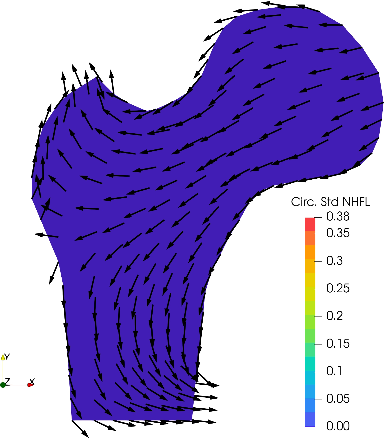
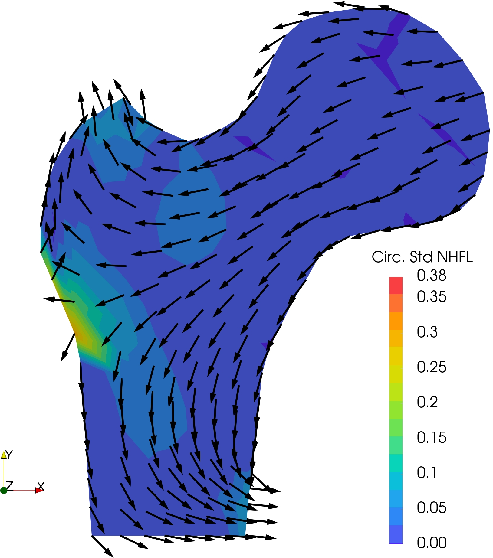
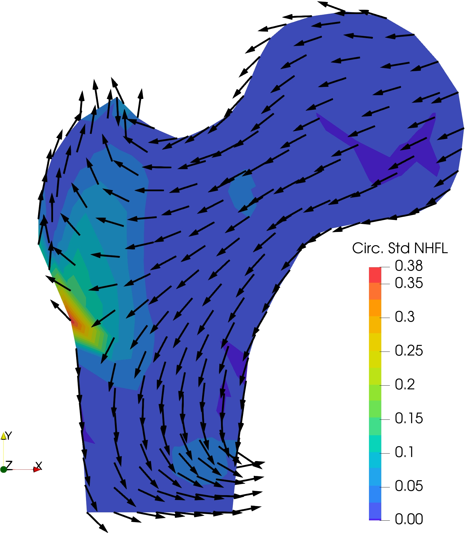
Apart from evaluating the statistics of magnitude of heat flux field , one may also be interested in understanding the statistics of direction of heat flow. To this, one may compute the second order circular statistics of the normalized heat flux, . Subsequently, the MC mean estimate of sampled unit vector field can be estimated accordingly [69, 54]:
| (46) |
where represents resultant Euclidean length of the sample mean , and is a unit vector defining the sample mean direction of . With the help of the former one, the sample circular standard deviation of can further be evaluated as
| (47) |
4.1 Results on 2D proximal femur
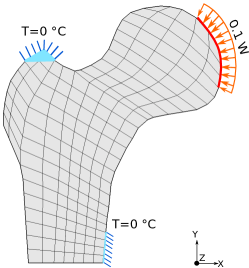
A two-dimensional proximal femur with a body of approximately 7 cm in width and 21.7 cm in height is considered, see Fig.1. A uniformly distributed surface heat flux with a resultant heating of 0.1 W and a fixed temperature of are applied at locations as shown in Fig.1. The computational domain is discretized by the finite element discretization method with 171 four-noded plane-stress elements, giving a mesh with 206 nodes and 390 degrees of freedom. In this study, each deterministic simulation obtained by sampling the stochastic parametric space is solved by the Calculix solver [20]. For the MC simulation, the Pearson coefficient of dispersion (for the scaling uncertainty) and samples are considered for all the cases in this study.
For simplification, we use abbreviations defined in Table 1 which are used to refer different modelling scenarios considered in this study. Each model will have a unique name in the form: reference tensor symmetry-realisation symmetry-type of model. For instance, “iso-ortho-scl” represents a model with random scaling only, such that the reference tensor belongs to isotropic symmetry, whereas the realisations are of orthotropic symmetry. Three such possible scenarios are explored in this article—“iso-iso-scl” (isotropy-isotropy-random scaling), “iso-ortho-scl” (isotropy-orthotropy-random scaling), and “ortho-ortho-dir” (orthotropy-orthotropy-random direction).
|
Type of model | ||||
|---|---|---|---|---|---|
| isotropy | orthotropy |
|
|
||
| iso | ortho | scl | dir | ||
Consequently, using the subscripts defined in Section 3.2 for random scaling and random orientation, two reference conductivity tensors— belonging to the isotropic symmetry class (denoted by superscript ) and with orthotropic symmetry (with superscript )—are considered, whose values are tabulated in Table 2. Furthermore, we simulate the grain orientations of the femur in a spatially homogeneous sense. As a result, the eigenvectors of the tensor corresponding to the eigenvalues and are oriented at an angle of in a clockwise direction to the x and y-axis, respectively.
|
|
||||
| Eigenvalues (W/mK) | |||||
|
|
||||
Random scaling with fixed symmetry:
the first modelling scenario is the one in which we perform random scaling only, such that the reference tensor , as well as the realisations, belong to isotropic symmetry (denoted by iso-iso-scl); see Fig.2 for a schematic overview of the model. In such a case, the random tensor is modelled—as in Eq.(22) —with random scaling only. Here the uncertain scaling parameters are modelled as identical log-normal random variables. Their corresponding PDF s are shown in Fig.2(a). A geometrically equivalent (circular) representation of reference tensor and realisations , where the radius of circle is defined by and [63], is presented in Fig.2(b). As can be seen the preservation of isotropic symmetry is apparent given the constant circular shape among the random variable realisations. However, the varying size of circles signifies a variation in scaling parameters.
Random scaling with varying symmetry:
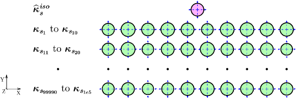
in the next scenario, we consider a similar stochastic tensor as described previously with a similar reference tensor . The difference being that the eigenvalues are modelled as independent identically distributed (i.i.d.) log-normal random variables. Due to which the realisations of model belong to orthotropic symmetry, thus, this model is denoted as iso-ortho-scl. Furthermore, in orthotropic realisations, the eigenvectors of related to random eigenvalues and are constrained at an angle of in clockwise direction with respect to x and y-axis respectively. The schematic representation of this model with varying symmetry is displayed in Fig.3, in which the corresponding PDF s are shown in Fig.3(a). Closer inspection of the Fig.3(b) shows the shift from circular geometry of isotropic reference tensor to orthotropic elliptical shape in realisations. One may also notice the variation in size of ellipses in the realisations as the semi-axes of ellipse are determined by and .
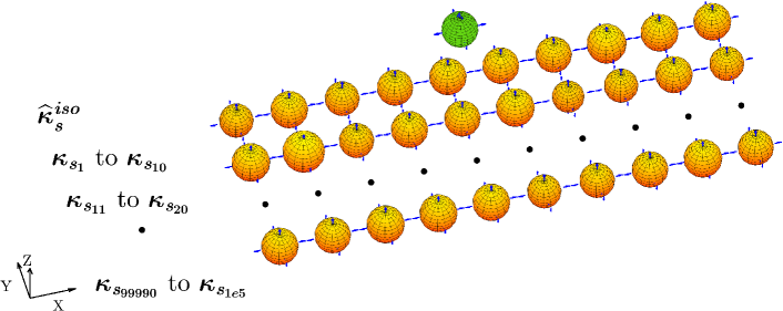
Random direction with fixed symmetry:
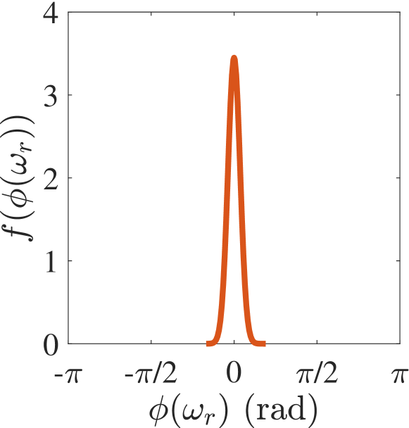
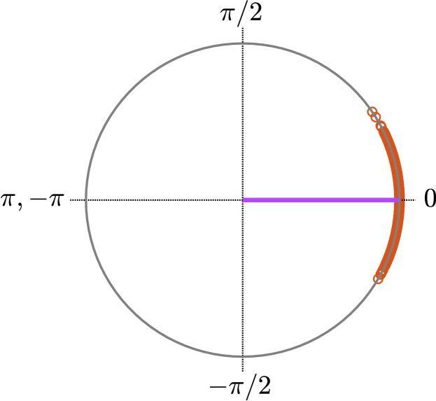
in the last modelling scenario, we build a random tensor , i.e. the exponential mapping of stochastic tensor as shown in Eq.(24), with random orientation only, given the reference tensor . Here the model is designated as ortho-ortho-dir, since, a fixed orthotropic symmetry is preserved in mean and realisations. The random angle of rotation is modelled as a von Mises random variable (see Eq.(42)) with zero mean with respect to x-axis and concentration parameter . In Fig.4(a), the PDF is shown on a real line over the domain , whereas the realisations of random variable and its sample mean vector (solid straight line) are plotted on a unit circle in Fig.4(b). In this study, we model directional uncertainty on the plane with as the axis of rotation. Thereby, the corresponding random rotation matrix in Eq.(24) takes the form:
| (48) |
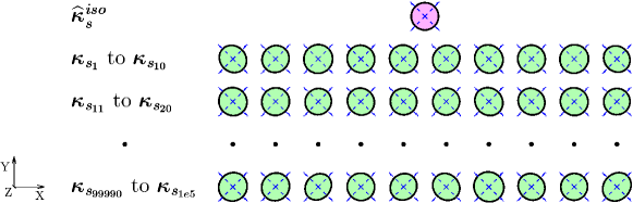
Here we consider a right-handed Cartesian coordinate system, meaning that positive values of random variable indicate counterclockwise rotation and vice versa. Fig.4(c) depicts the corresponding elliptical geometric visualization of the model. As can be seen that the orientation of elliptical semi-axes fluctuates in the realisations , whereas its size and shape remain constant in the mean and realisations.
Uncertainty quantification:
Fig.5 shows the MC mean estimate of the nodal temperature (NT) for the three described stochastic models. For easier interpretation, in this study, the results are displayed on a uniform scale. Hence, the values range from zero to a maximum value (corresponding to a given estimate of the desired output quantity). Clearly, the results in Figs.5(a) and 5(b) are similar, as the considered reference tensor is identical in both the cases. Due to the assumption of an orthotropic mean tensor , in the third figure Fig.5(c), we see a significant difference in the magnitude/contour pattern of the temperature.
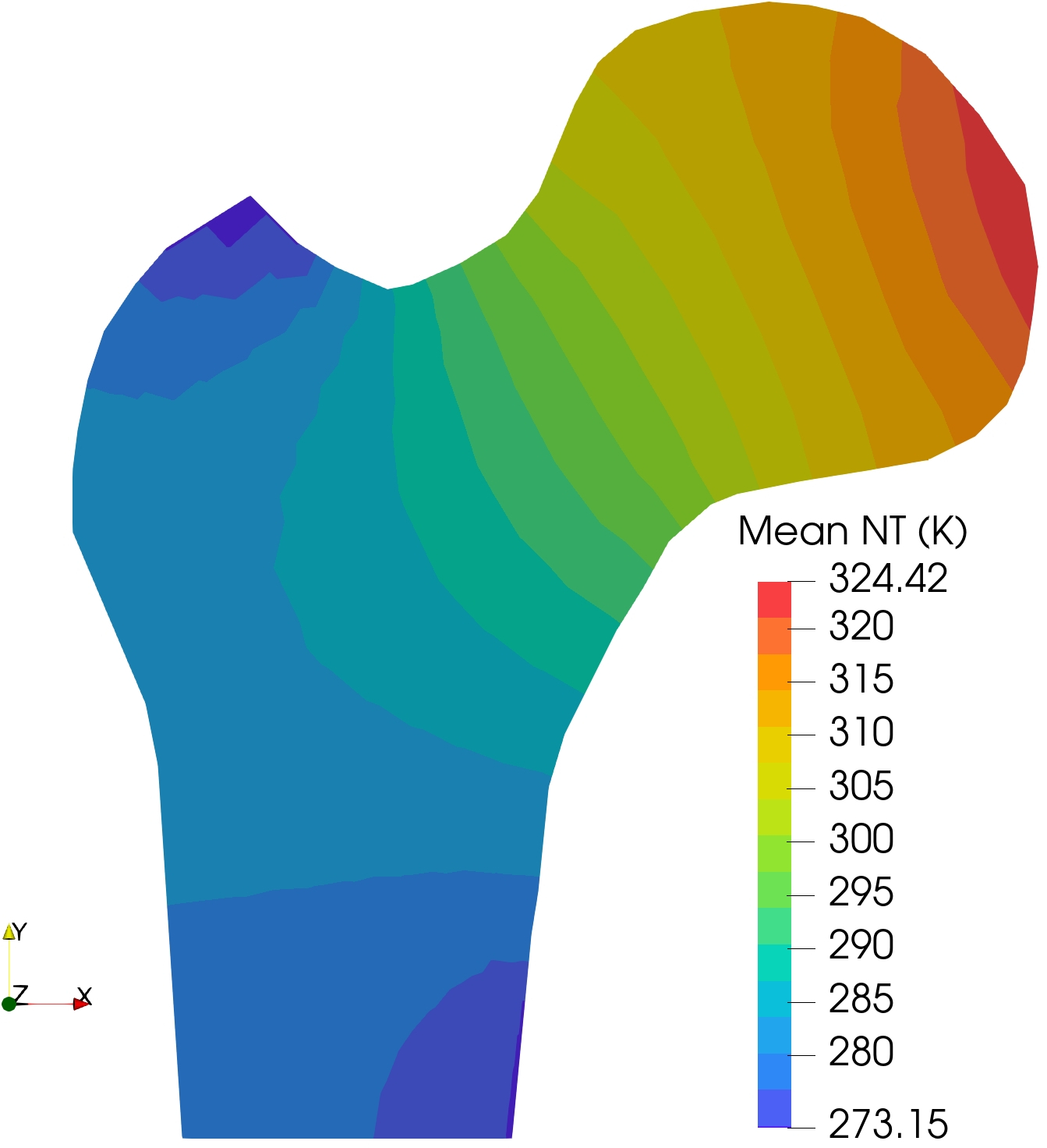
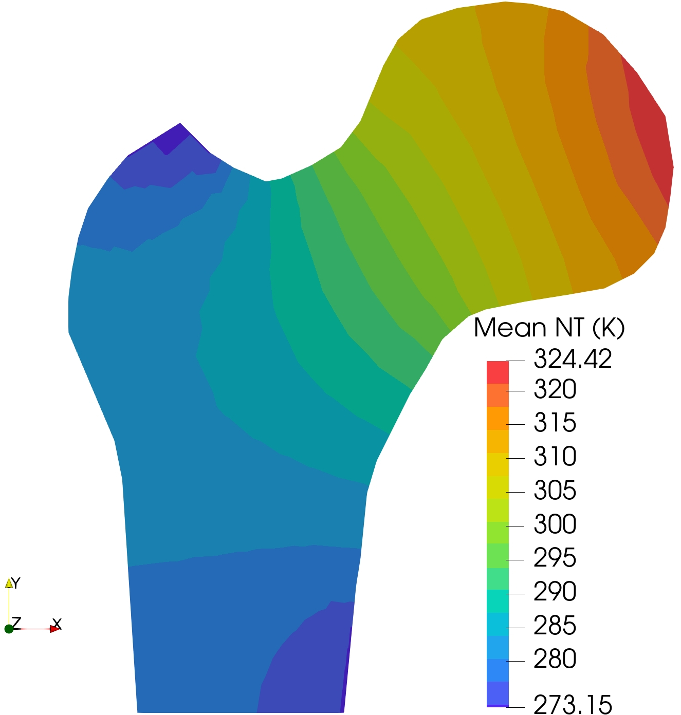
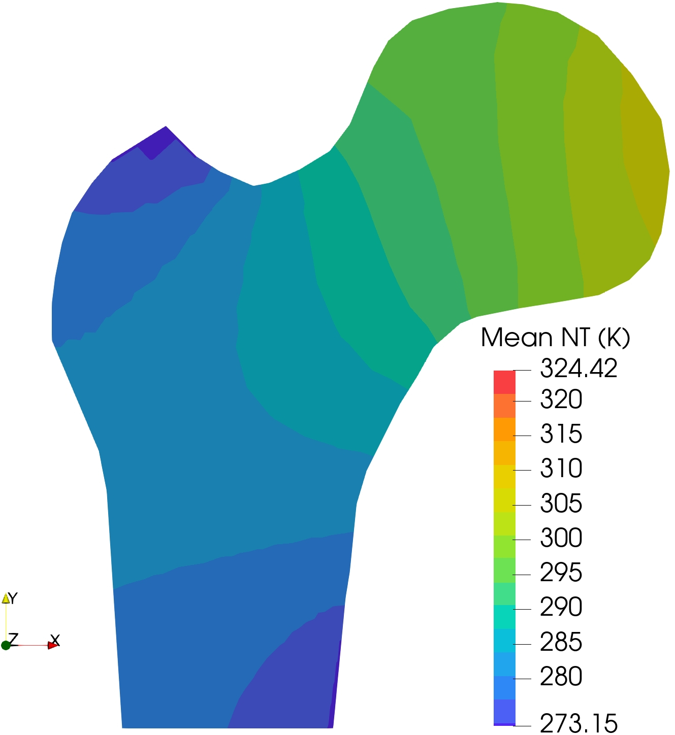
Fig.6 further depicts the standard deviation of temperature . Due to different modelling assumptions, it is apparent that all three results in this figure are different from each other. But Fig.6(c) stands out the most, where the stochastic influence on nodal temperature is much lower as compared to the other two cases.
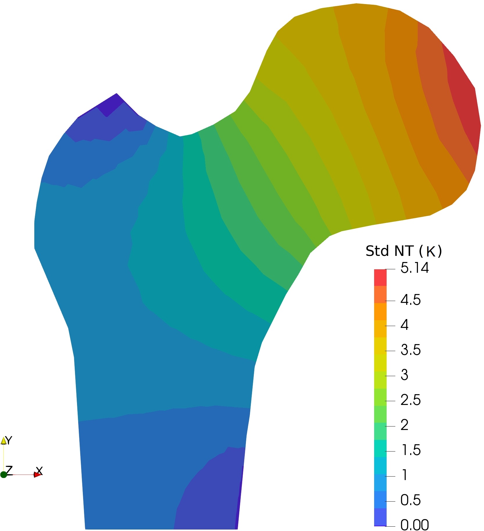
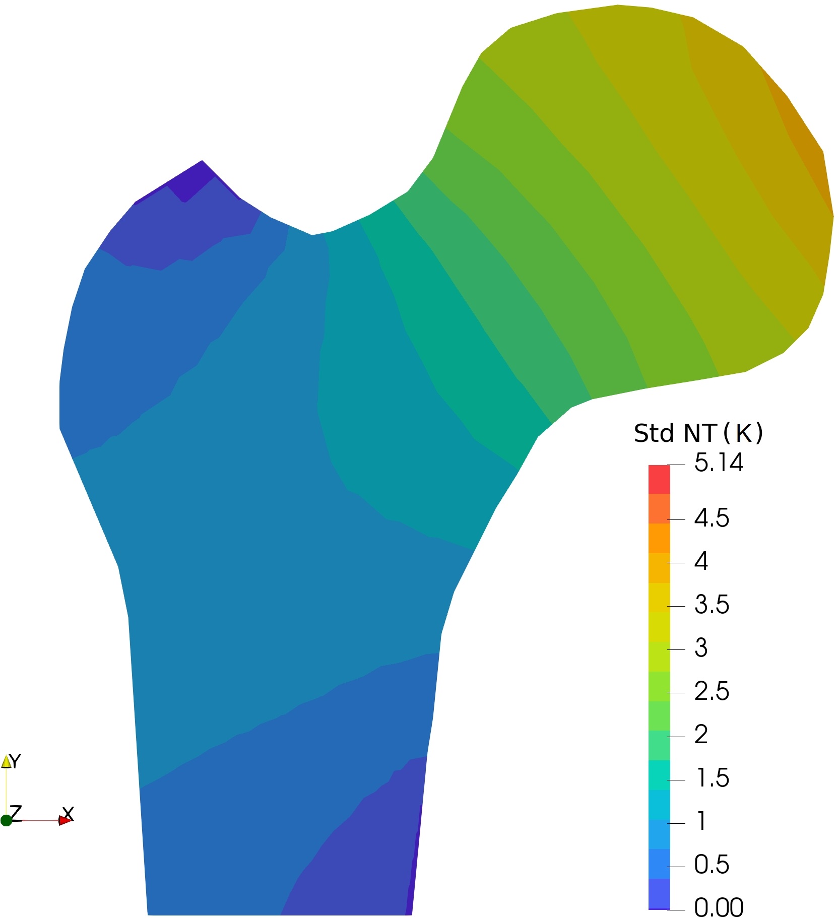
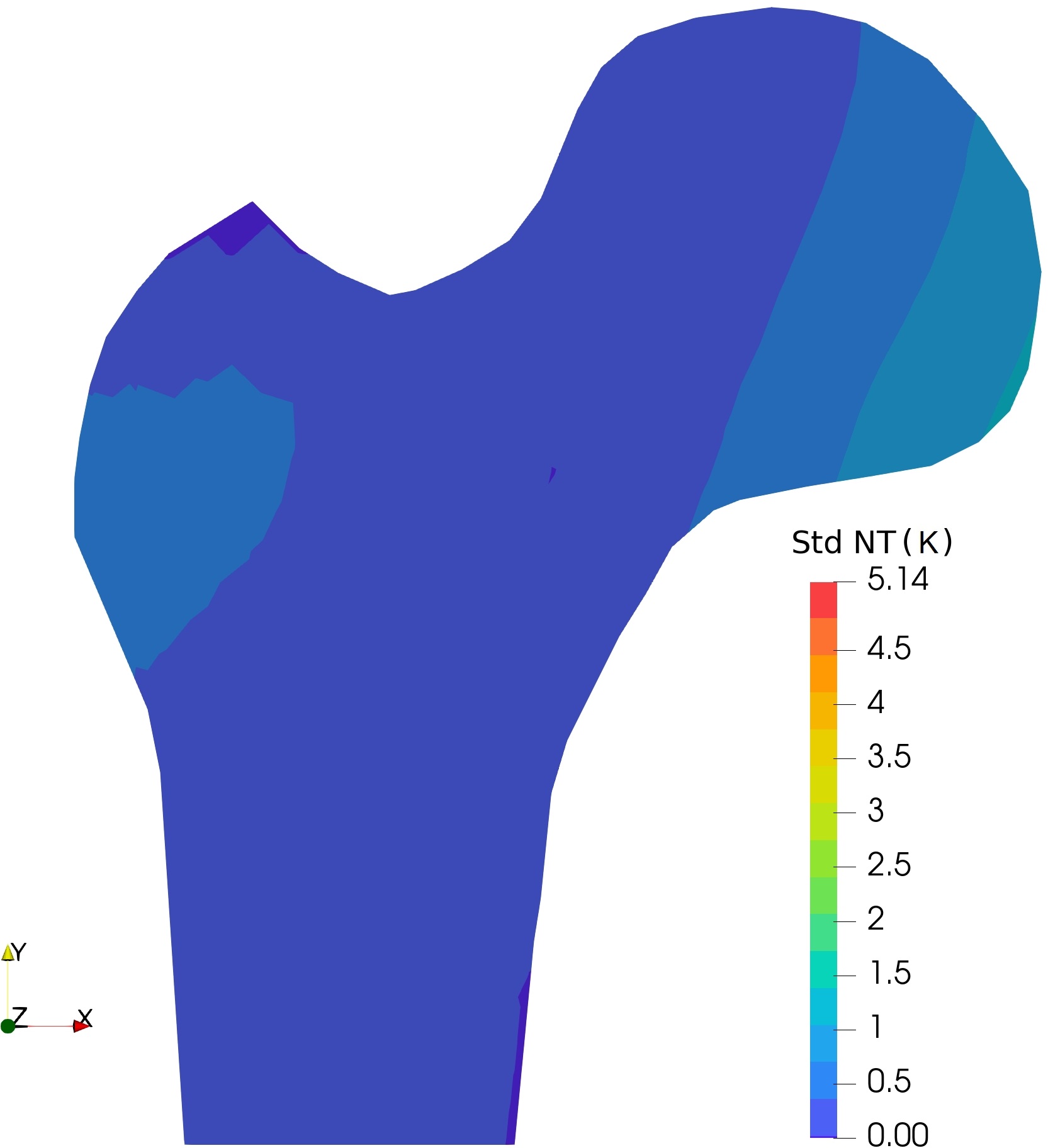
In the first two scenarios, only the scaling parameter is uncertain, whereas in the third example we consider only directional uncertainty. We know that under the assumption of deterministic boundary conditions, the random temperature field varies inversely to the stochastic coefficeint . As the scaling parameters of the model remain constant, the impact on the variation of temperature field due to directional randomness is small. On the other hand, when the scaling parameters are modelled as varying, the standard deviation estimate of temperature becomes more sensitive as evident in Figs.6(a) and 6(b). Interestingly, when Fig.6(b) is compared to Fig.6(a), it is clear that, varying the material symmetry from higher (isotropy) to lower (orthotropy) order in the model iso-ortho-scl results in lower stochastic influence on temperature .

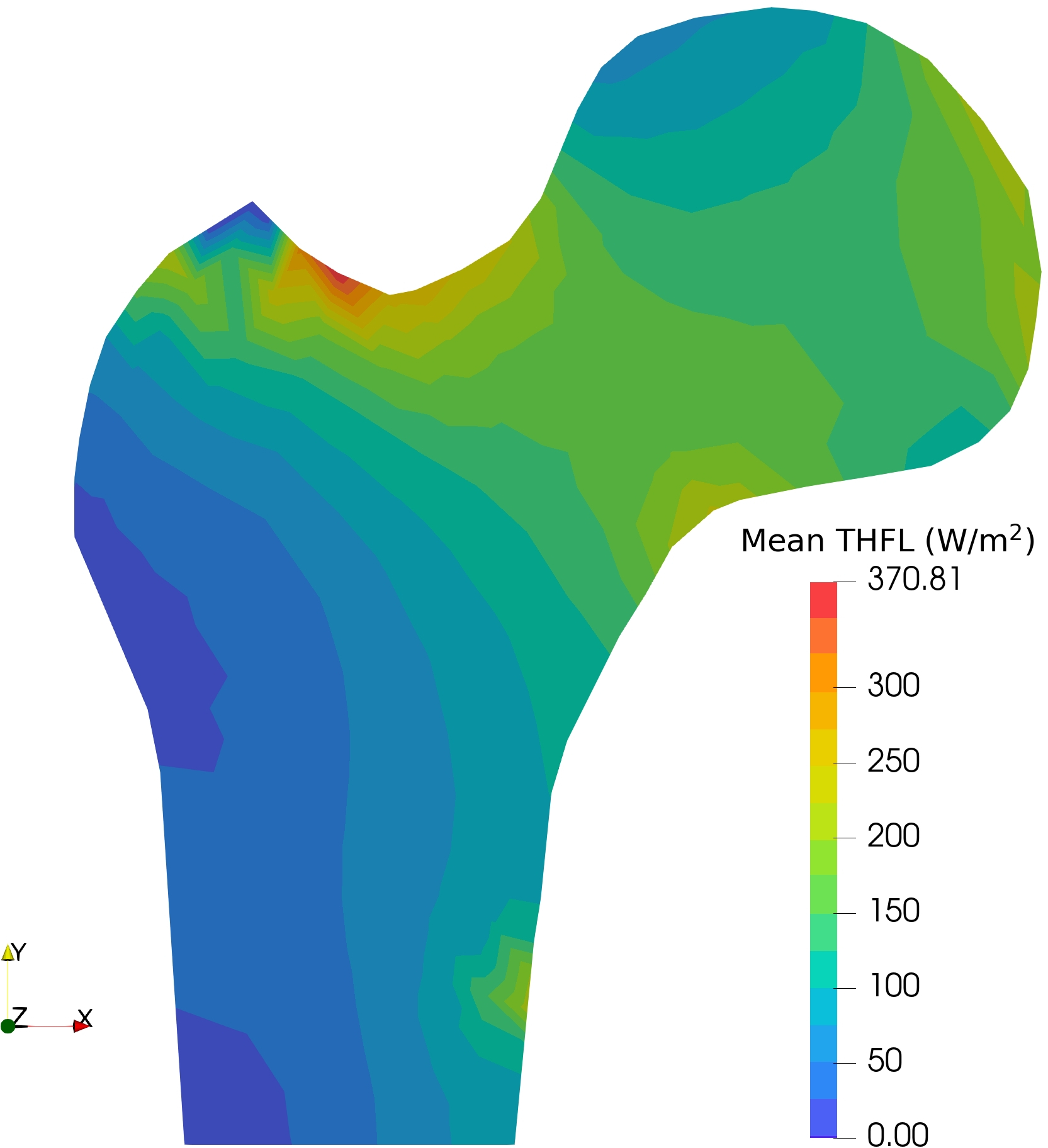

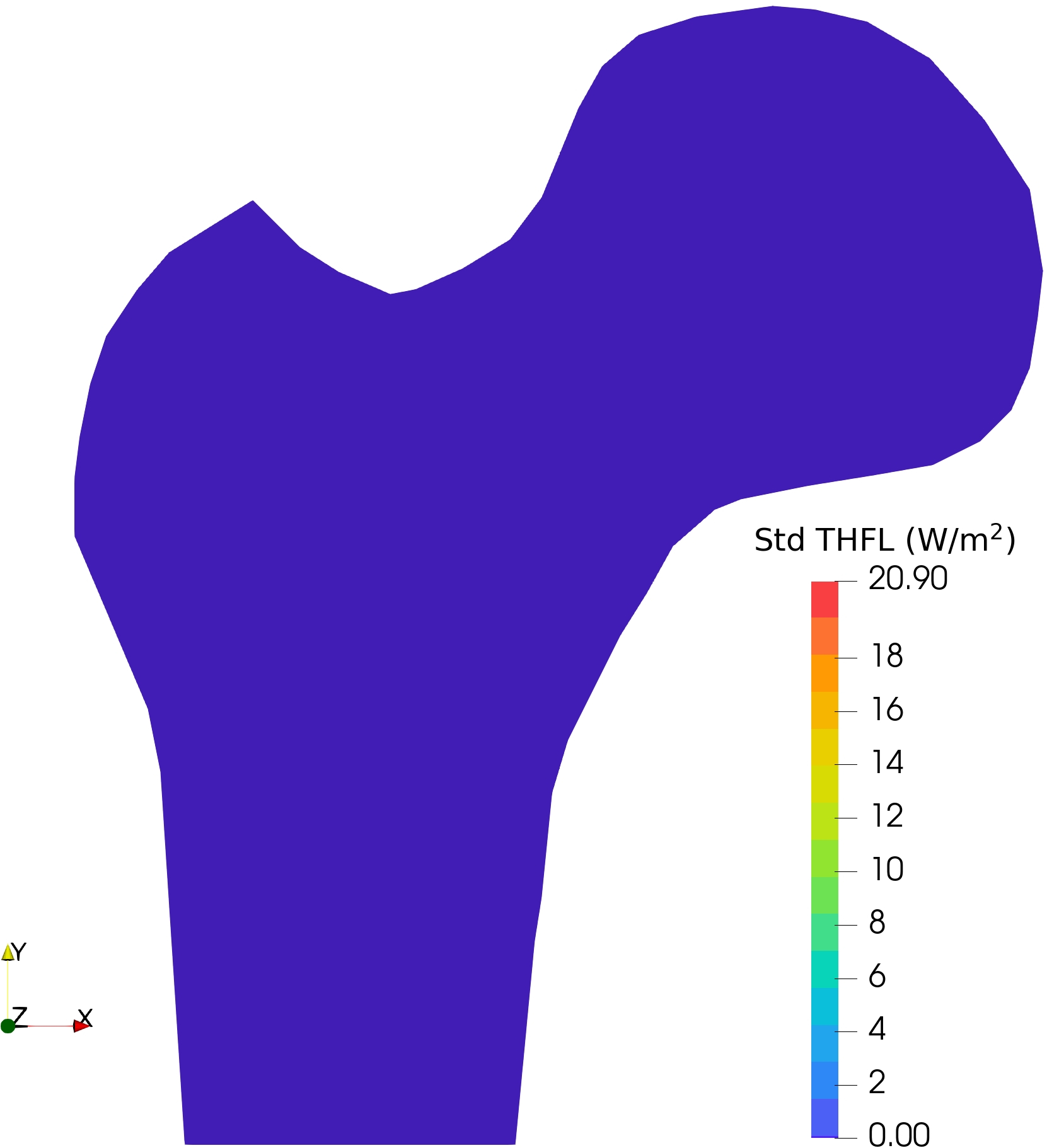
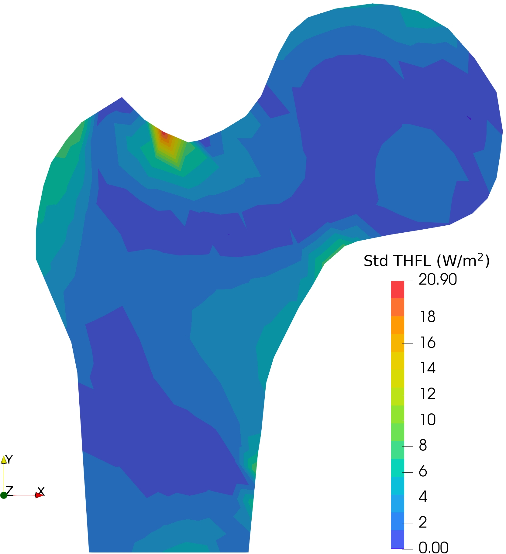
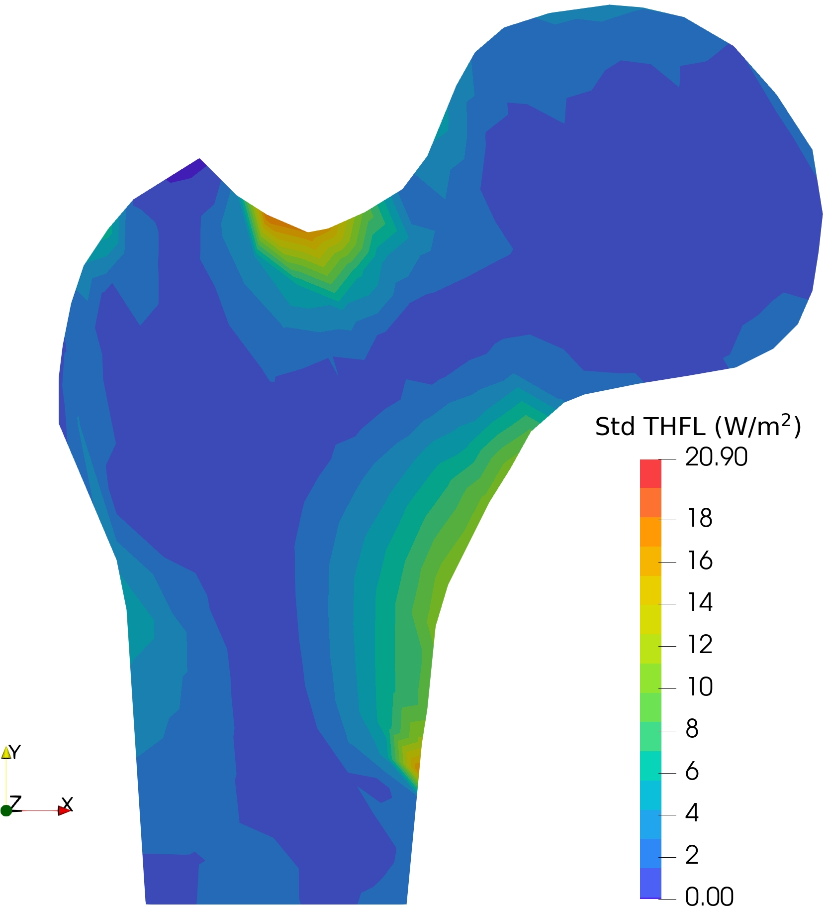
Furthermore, the sample mean estimates of total heat flux (THFL) are presented in Fig.7, where, Figs.7(a) and 7(b) showcase similar results as described previously (see Figs.5(a) and 5(b)). However, in comparison to these two figures, a visible difference in maximum total heat flux and contour pattern is noticed in Fig.7(c). In Fig.8, the corresponding estimated standard deviation of THFL is plotted. Here, the most interesting aspect is seen in Fig.8(a), where, the standard deviation is close to zero. It turns out that, in the model iso-iso-scl, the stochastic coefficient has almost perfect inverse correlation with temperature gradient field . Thus, the randomness in the model has almost no stochastic impact on THFL . However, on the contrary, the estimate in Figs.8(b) and 8(c) is visible, signifying the stochastic influence of the considered input models on THFL . One may conclude that directivity has more impact on the heat flux than the scaling parameter.
Additionally, the directional mean and standard deviation of normalized heat flux (NHFL)—from Eq.(46)—are displayed in Fig.9. The mean orientation (vector representation) in Figs.9(a) and 9(b) look similar, however, with a closer inspection of Fig.9(c), the difference is apparent. Similar to the results in Fig.8, the circular standard deviation estimate in Fig.9(a) is also close to zero, showing once again the insensitivity of directional attribute of NHFL to scaling uncertainty present in the model . Also, in comparison, the standard deviation estimate in Fig.9(c) is more significant than in Fig.9(b).
4.2 Results on 3D proximal femur
A three-dimensional proximal femur configuration of dimensions 45 mm in width and 154 mm in height is considered. The boundary conditions with identical values as used in the 2D example are imposed, shown in Fig.10. The computational domain is discretized by a four-noded tetrahedral finite element mesh, comprising 12504 nodes, 3166 elements and 35115 degrees of freedom.
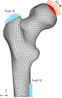
We use similar modelling scenarios as in 2D case i.e. iso-iso-scl, iso-ortho-scl and ortho-ortho-dir (see Table 1 for model abbreviations). The considered isotropic and orthotropic reference conductivity tensors are tabulated in Table 3. Furthermore, by fixing the negative y-axis as the rotational axis, the directional vectors of the model corresponding to the eigenvalues and are positioned at an angle of in an anti-clockwise direction with respect to the and -axis, respectively.
|
|
||||
| Eigenvalues (W/mK) | |||||
|
|
||||
Random scaling with fixed symmetry:
A stochastic tensor with fixed symmetry (iso-iso-scl), where the random scaling elements are modelled by an identical log-normal random variable, is constructed. The schematic representation of the model is shown in Fig.11, where Fig.11(a) presents the log-normal PDF of scaling parameters , whereas the geometric visualization—in the form of equivalent spheres—of the reference tensor and realisations is displayed in Fig.11(b). Here the radius of the sphere is determined by , and . As can be seen that the radius of the spheres in the realisations vary and the spherical shape of the mean is maintained in the realisations, owing to the preservation of isotropic material symmetry in the mean and realisations.
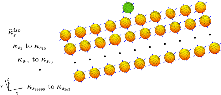
Random scaling with varying symmetry:
a random tensor model similar to the previous scenario, however with a varying material symmetry (iso-ortho-scl) is showcased in Fig.12. In Fig.12(a), the PDF of i.i.d log-normal scaling parameters can be seen, whereas Fig.12(b) shows the geometric interpretation of the mean and realisations . Looking from the negative y-axis, the eigenvectors of the model conforming to the eigenvalues and are at an angle of in an anti-clockwise direction corresponding to x and z-axis, respectively. A change in symmetry from isotropic in the mean (spherical shape) to orthotropic (ellipsoidal shape) in the realisations is evident. Also, the fluctuation in lengths of semi-major axes—calculated by , and —of the ellipsoids represents the aspect of varying scaling parameters.
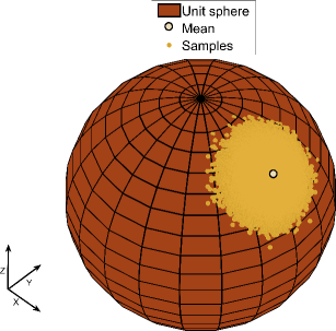
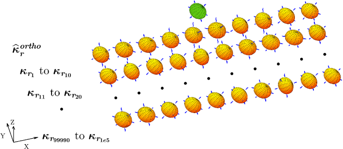
Random orientation with fixed symmetry: to account for directional uncertainty only, a random tensor with fixed symmetry (ortho-ortho-dir) , which is the exponential of the model described in Eq.(24), is considered. The eigenvector of random tensor related to the eigenvalue is modelled as a von Mises-Fisher distribution (see Eq.(41)) with the mean direction (the eigenvector of the reference tensor which corresponds to the eigenvalue ), and the concentration parameter . The random rotational angle is determined using the dot product operation, , whereas the unit random rotational axis is evaluated by the cross-product operation, . The corresponding random rotation matrix is then modelled as per the Rodrigues rotation formaula, described in Eq.(29). Fig.13 summarizes the model . Here Fig.13(a) displays the mean and realisations of von Mises Fisher random variable on unit sphere; the equivalent ellipsoidal representation of stochastic model is portrayed in Fig.13(b). It is evident that the shape and size of the ellipsoid in the mean and realisations remain constant; only the orientation of semi-axes of ellipsoids in the realisations fluctuate.
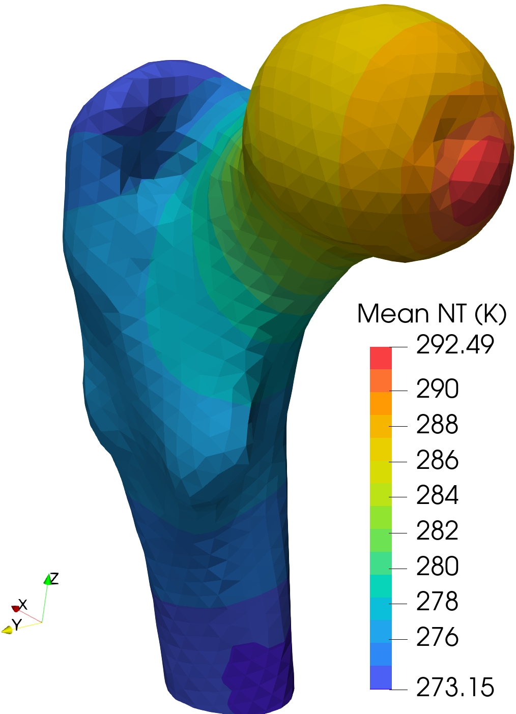
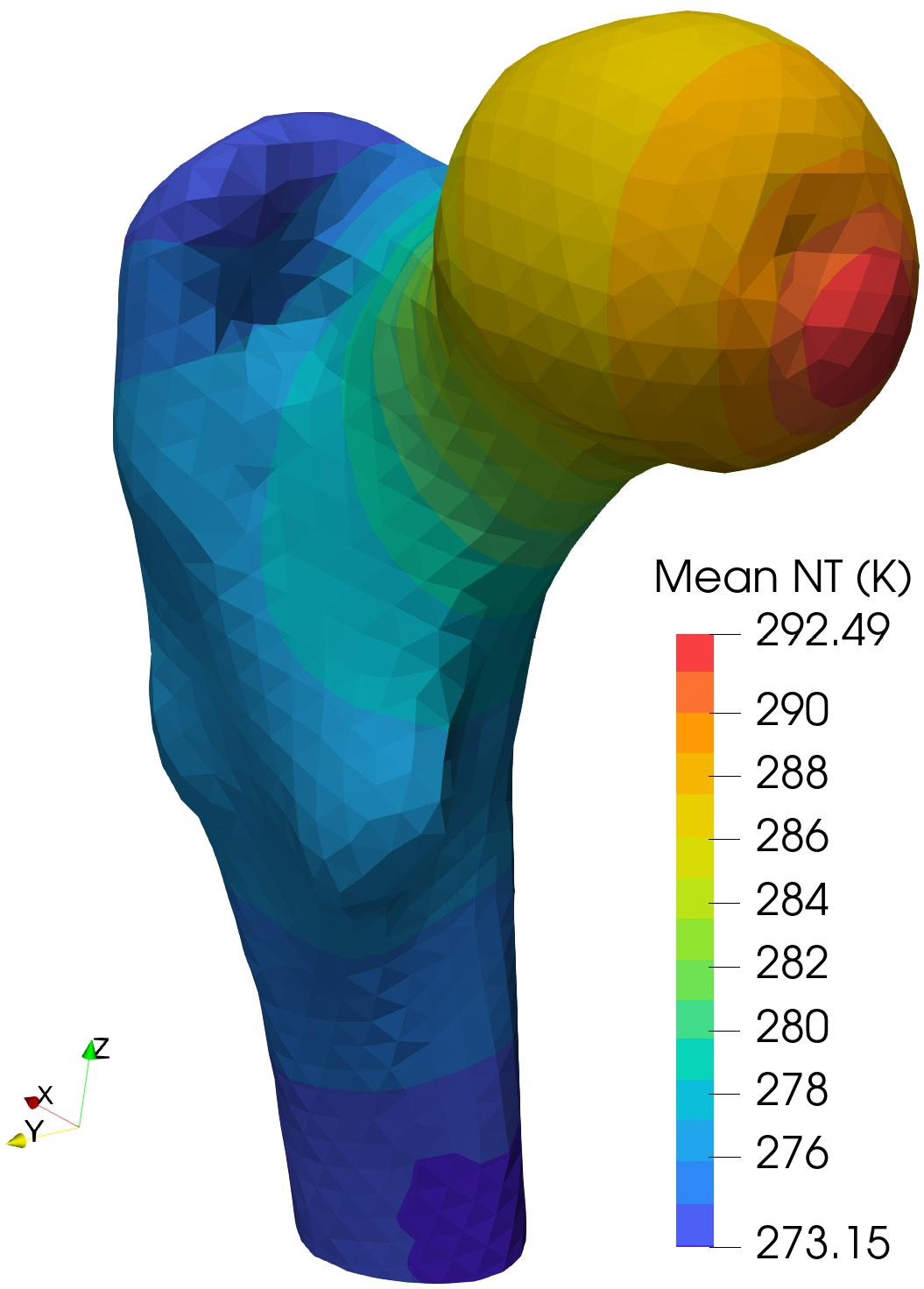
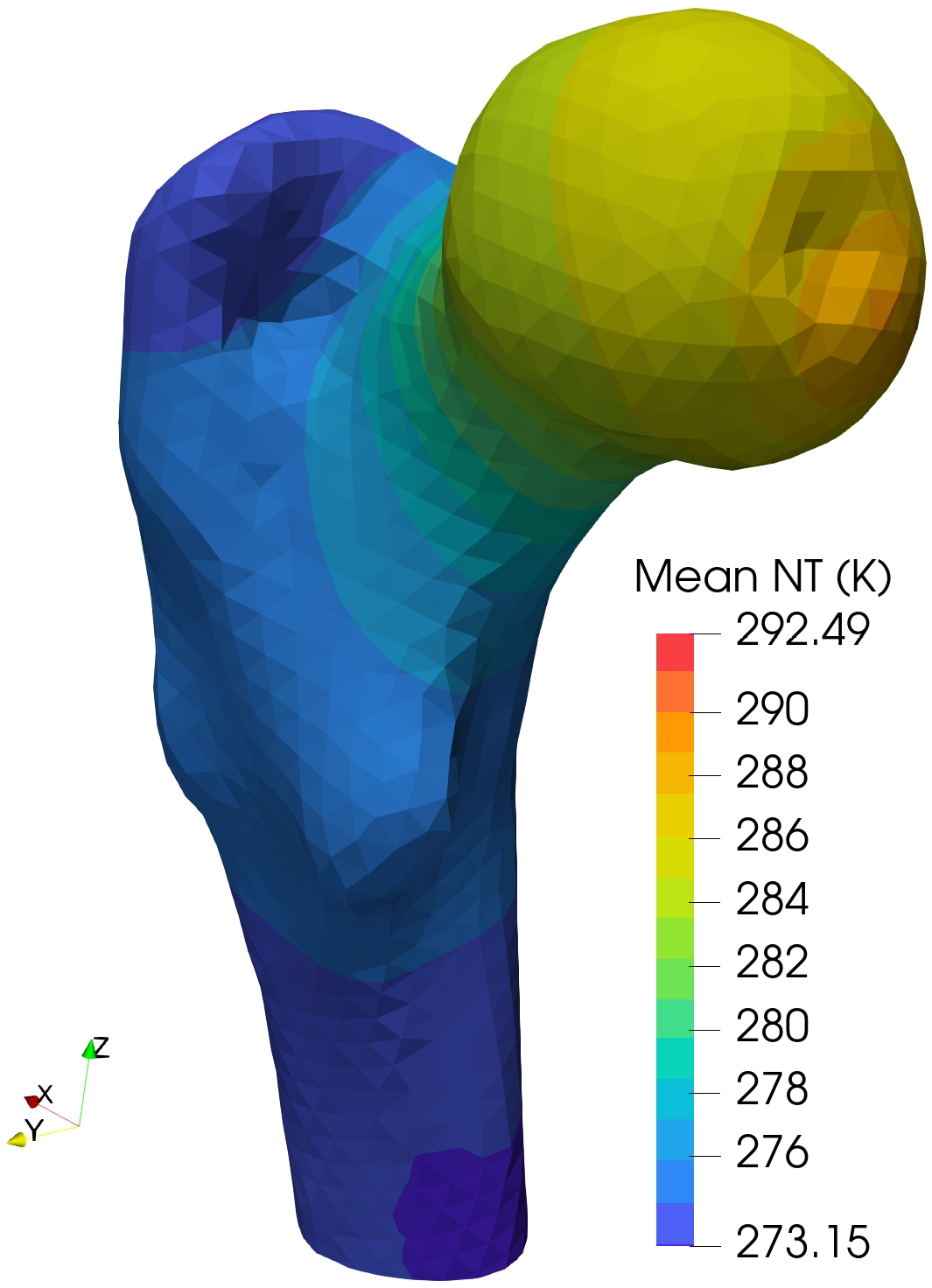
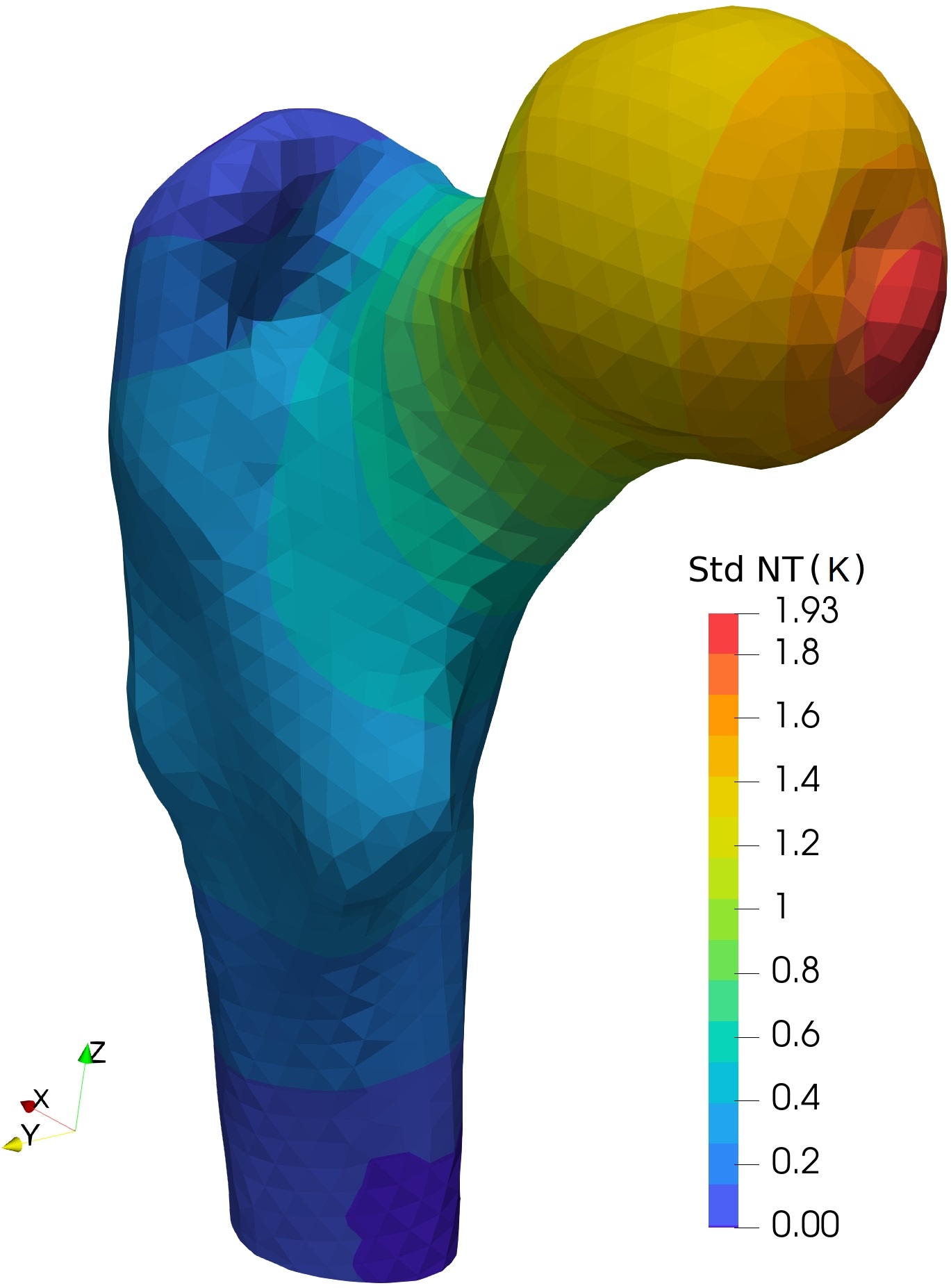
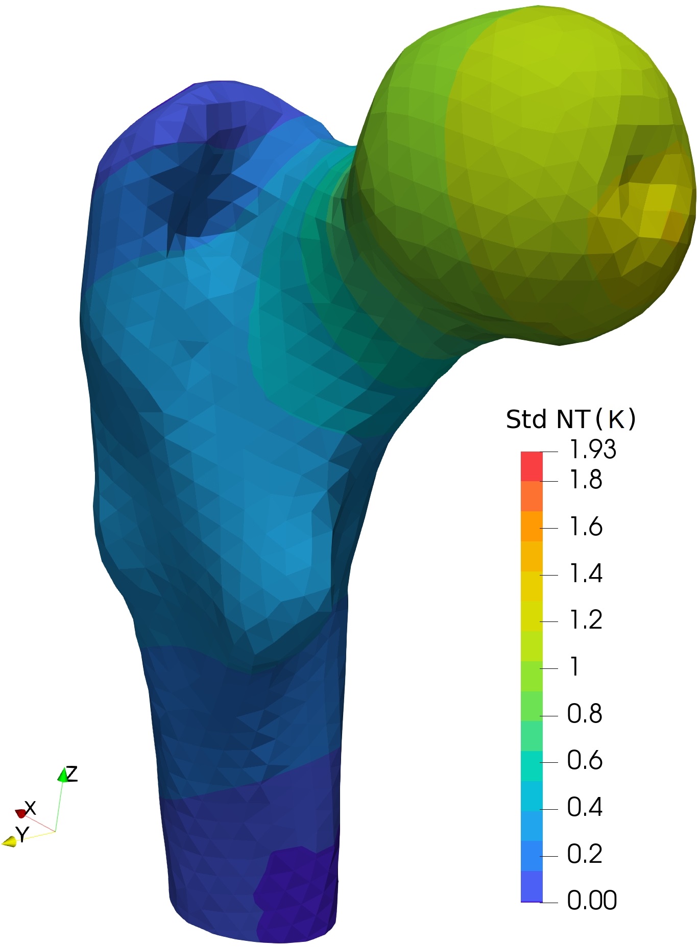
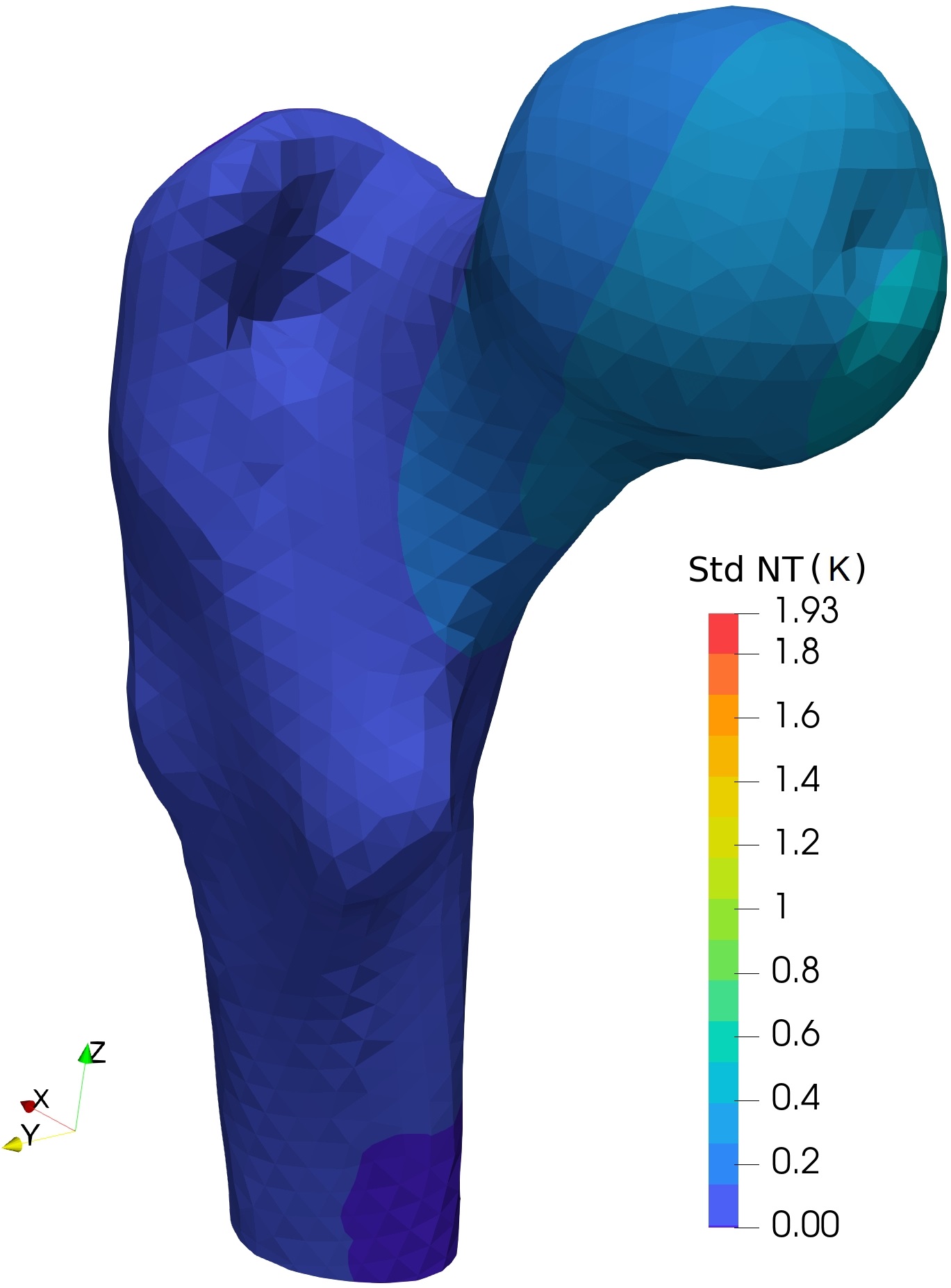
Uncertainty quantification
: Figs.14–17 display the MC mean and standard deviation estimates of NT and THFL, whereas Fig.18 shows the circular MC mean and circular standard deviation estimate of NHFL. Concerning the sensitivity of different stochastic models on the desired quantities, we make similar observations, and hence, draw similar conclusions on the 3D example as in the previous 2D case (from Section 4.1). That is, the findings in Figs.5–9 correspond approximately to the results in Figs.14–18.
The numerical results of both 2D and 3D proximal femur signify the prominence of incorporating different material uncertainties—scaling, orientation and material symmetry—independently into the constitutive model; the results showcase the distinct impact of stochastic models on the desired quantities of interest, such as nodal temperature and heat flux.
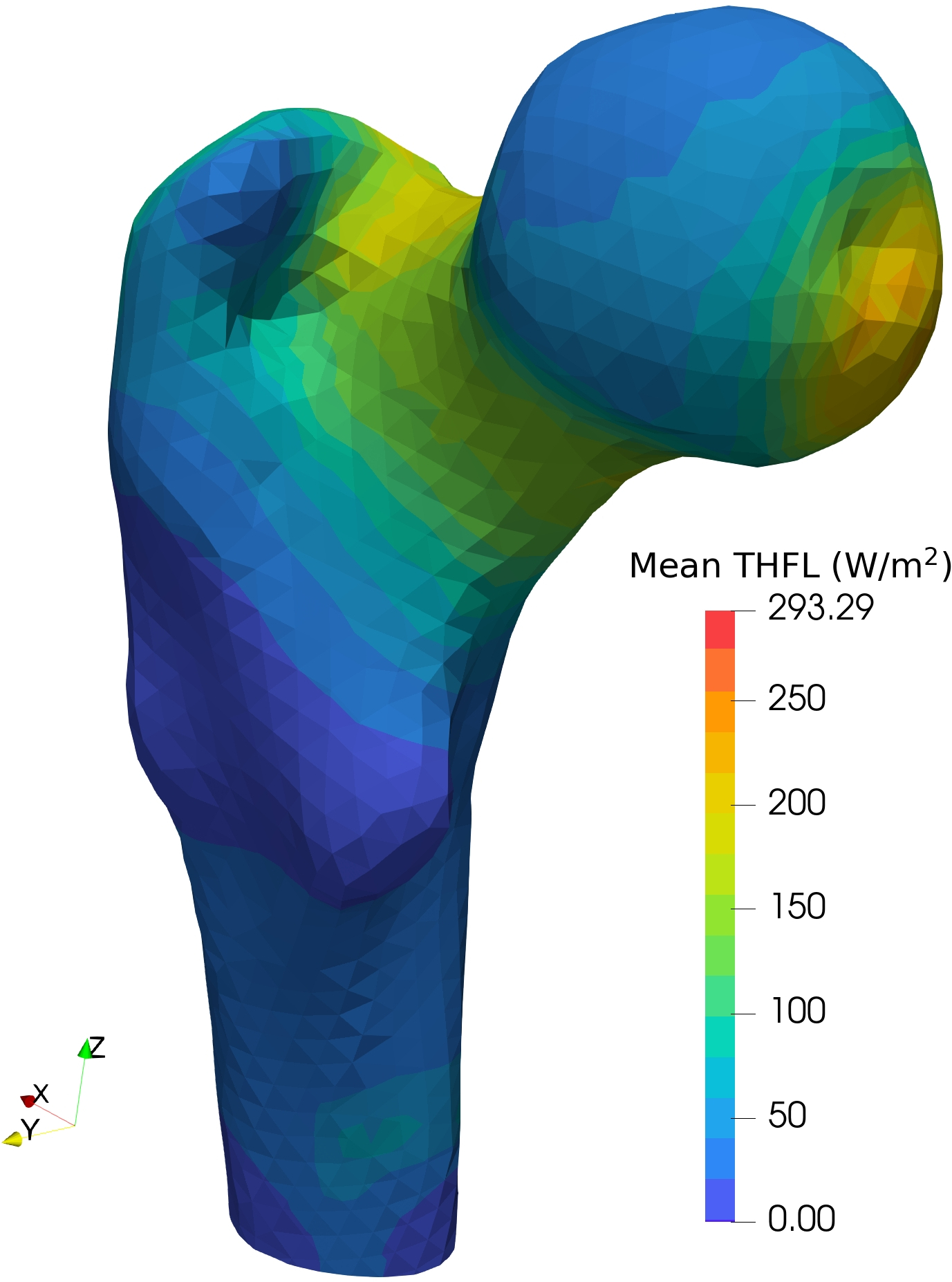


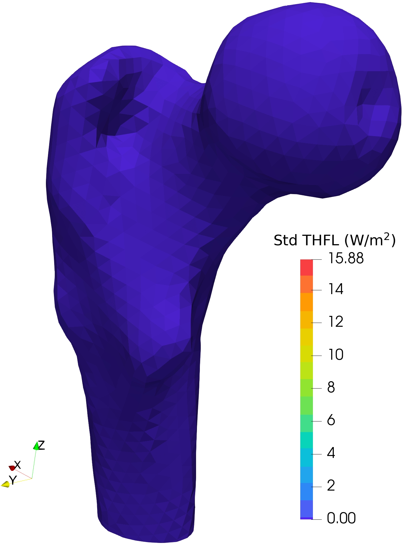

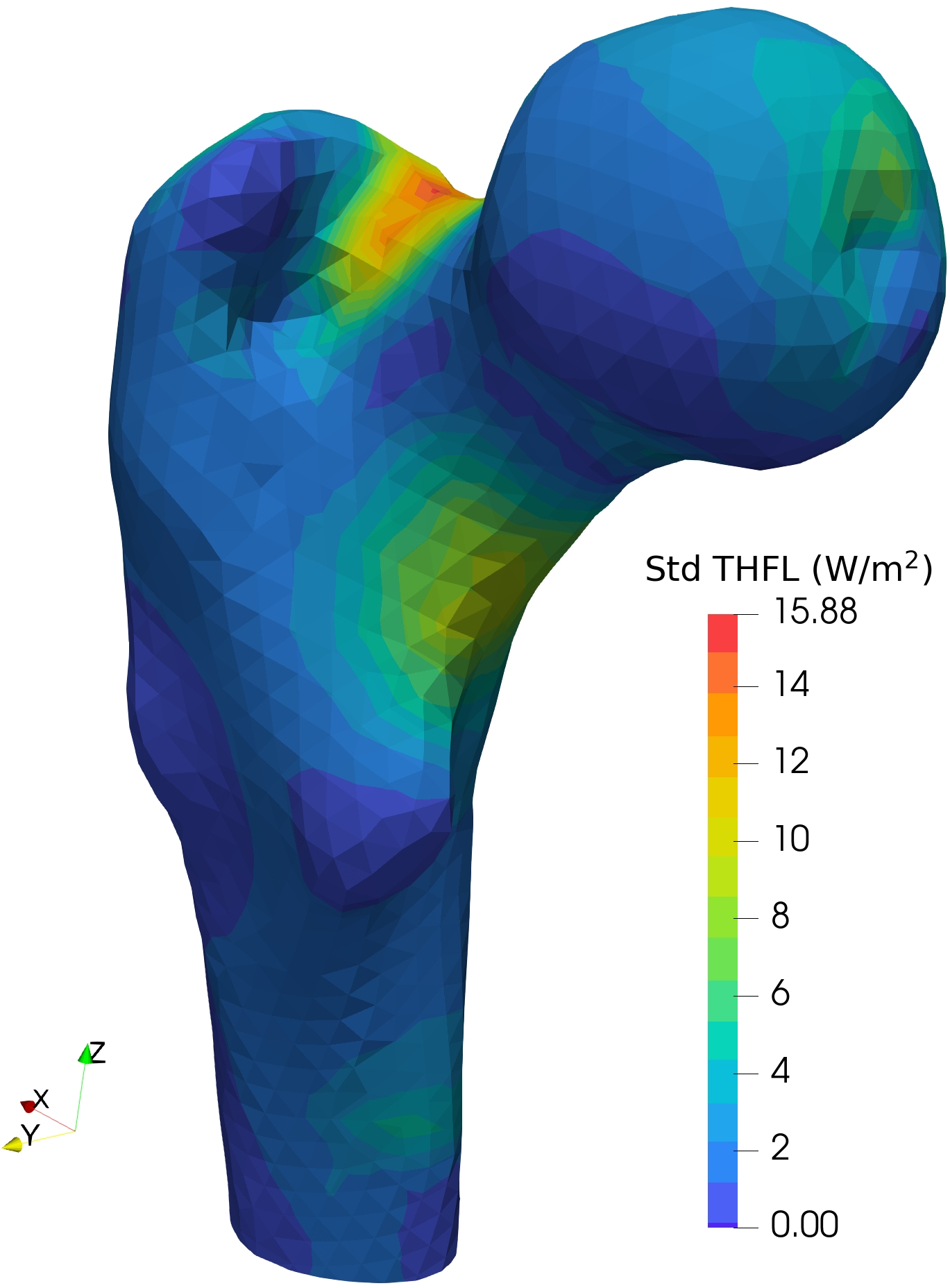
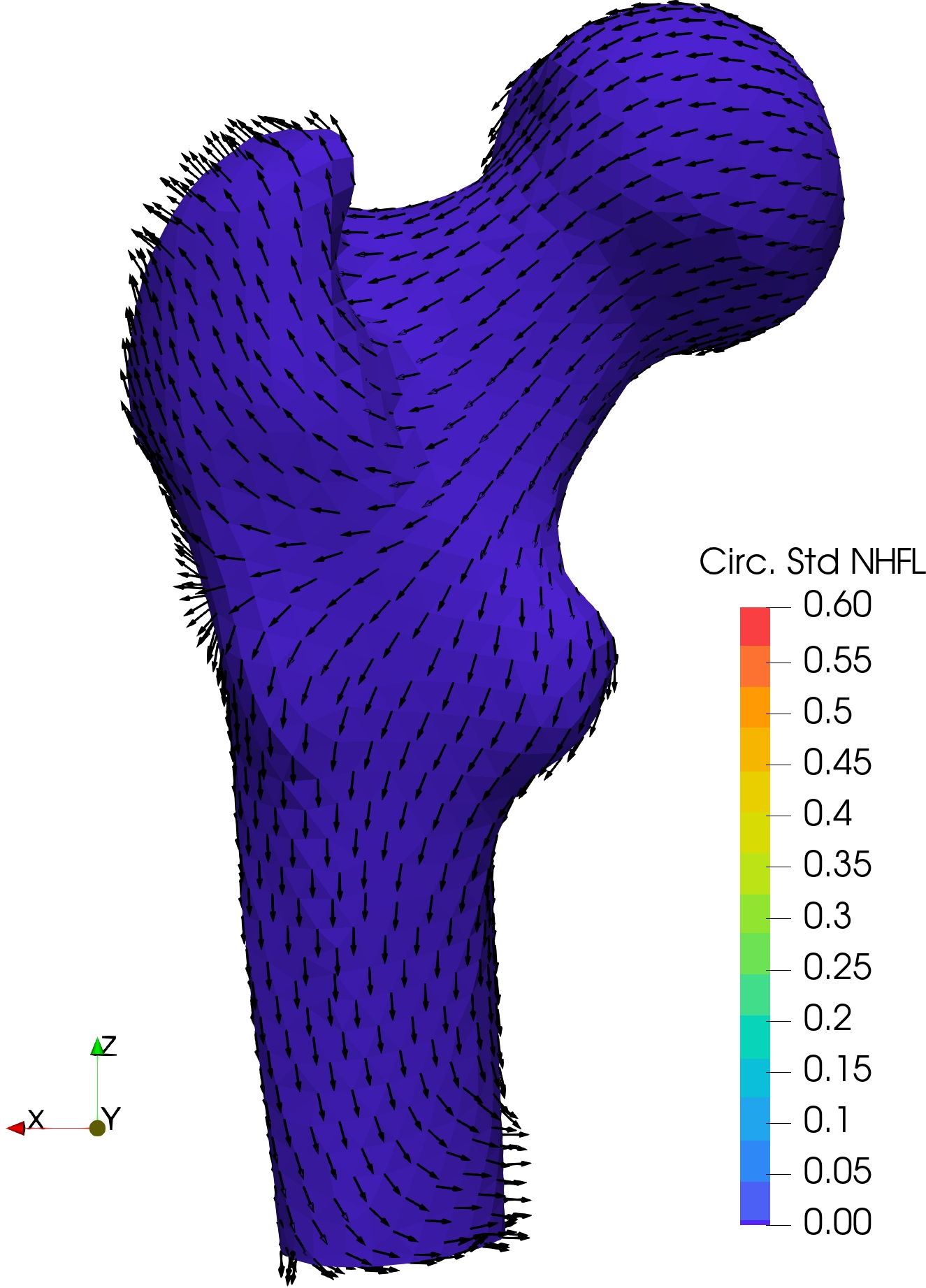
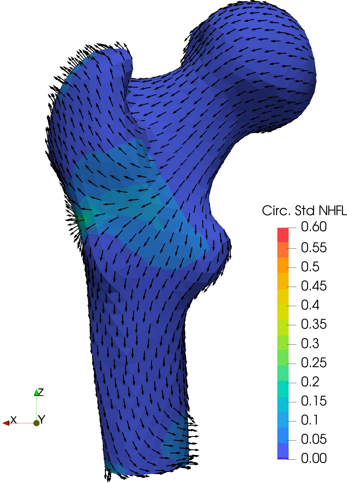
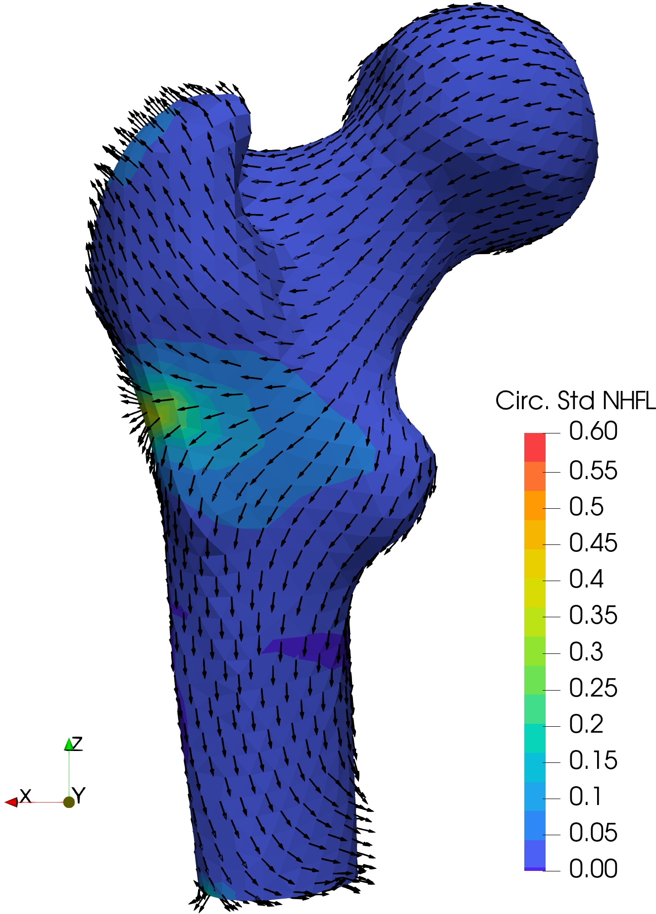
5 Conclusion
Here the task of modelling and representing random symmetric and positive definite (SPD) tensors was addressed, and some desiderata for the modelling and representation were formulated. Namely, the representation has to be SPD even under numerical approximation, and has to be such that one is able to control the material or spatial invariance resp. symmetry, both for each possible realisation and for the the expected value. Regarding the mean or expected value, it turned out that the usual expectation, which is tied to the structure of a linear space, may not be appropriate on the open convex cone of SPD tensors. The more general Fréchet mean is based on distance measurements, possibly different from the usual Euclidean distance, on the set of SPD tensors. Here some desiderata were formulated for the distance measure, which take into account the physical purpose and uncertainty involved in stochastic models of such physically symmetric and positive definite tensors.
Therefore in Appendix A the type of metric that one can consider for symmetric positive tensors and specifically for the set of SPD matrices to compute the correspondin Fréchet mean is discussed. As the Euclidean mean suffers from the so-called swelling effect, we suggest alternatives such as the geometric, log-Euclidean, and scale-rotation separated mean.
It was also proposed to follow a widely used technique to model and represent the logarithm of tensor, such that the symmetric positive definite attribute is automatically satisfied when taking the exponential in the end; the invariance properties automatically translate to the logarithm. To expose the ideas in the simplest possible setting, we consider specifically second-order SPD tensors, where the symmetry classes are quite simple.
More particularly, the focus is on modelling uncertainties in such a way as to have a fine control independently over the strength/scaling and directional attributes of the tensor—given that the material symmetry is fixed. As we separate the strength and orientations of the random SPD matrices by spectral decomposition, the task boils down to modelling the random scaling parameters of the logarithm of a random diagonal matrix, as well as the random orthogonal matrix of eigenvectors. Such orthogonal matrices are members of the Lie group , and the well-known exponential map from the corresponding Lie algebra of skew-symmetric matrices was used to carry random ensembles in the free vector space onto such ensembles on . This results in the random orientation being modelled by symmetric circular/spherical distributions. Furthermore, a scenario of fluctuating the material symmetry around the Fréchet mean is also studied, i.e. the mean tensor belongs to a higher order of material or spatial symmetry, whereas each realisation belongs to a lower order of material symmetry.
As an application in this study, the random thermal conductivity tensor of a steady-state heat conduction on a 2D and a 3D model of a proximal femur bone was investigated, a highly anisotropic material. Three different modelling scenarios are considered: random scalings only, random scalings with fluctuating symmetry, and random orientations only. The material uncertainties are then propagated to the output responses such as nodal temperature (NT), total heat flux (THFL)and normalized heat flux (NHFL)using the Monte Carlo method (MC). Subsequently, statistics such as mean and standard deviation estimates of NT and THFL, and circular mean and circular standard deviation estimates of NHFL are determined.
From the numerical results of both 2D and 3D models, it is clear that NT is most stochastically sensitive to the model with random scalings only, and least sensitive to random orientation only. On the other hand, the randomness in the model with random scaling only has almost zero stochastic influence on THFL—determined by the Euclidean norm—but the impact of the other two random models is evident. One may also observe a similar stochastic sensitivity of the stochastic models on NHFL, as well as on THFL. Therefore, the distinctive impact of the three stochastic models on the output response signifies the importance of incorporating different material uncertainties—scaling, orientations and material symmetry—independently into the constitutive model.
In total, we have proposed a modelling scenario for tensors defining positive-definite material properties which takes into account possible material resp. spatial invariances or symmetries. Our approach allows a fine control of the scaling randomness, and independently of the orientation randomness, further separating it into the invariance properties of the mean and those of the random fluctuations.
Appendix A Metrics on symmetric positive definite matrices
As was already noted in Section 1, positive definite tensors live geometrically on an open convex cone in the vector space of symmetric tensors . It is a differentiable manifold, but it is also part of the ambient space, the Euclidean resp. Frobenius or Hilbert-Schmidt norm. It has been found that this Euclidean metric on ,
| (49) |
namely
| (50) |
when used on the open convex cone [90, 1, 83, 2, 3, 22, 23, 31], leads to the undesirable swelling, fattening, and shrinking effects in interpolation resp. averaging [96, 57, 97, 38, 37, 27]. In addition, being an open subset means that is not metrically complete with the Euclidean metric , which in turn means that Cauchy sequences in in the metric may have limits which are not in , i.e. they could be singular, which may present a problem in approximation algorithms.
A.1 Metrics
What metric to take instead of the Euclidean one connected with the arithmetic mean is not so clear. For an overview of various options one may consult [85], see also the discussion in [38, 91]. Most proposals turn , which as an open subset of the linear vector space carries a natural structure of a differential manifold, into a Riemannian manifold in different ways with different metrics. This allows to measure the lengths of continuous paths in , thus leading to shortest paths or geodesics, on which one can naturally define interpolants resp. averages. A good introduction to this very active subject [105, 106, 107] relating to metrics on may be found in the collection [91], see also [85, 27, 39].
As will be seen, the open convex cone may be considered as a metric space in ways different from just being a subset of the vector space . In addition to the desiderata listed in Section 2 for a metric, and connected obviously to the first requirement, one may want that as for any , but the same should also hold as , in fact singular matrices in should all be infinitely far away from the identity, i.e. all of the boundary should be at an infinite distance from the identity.
A.2 Affine-invariant distance
The best known alternative to the Euclidean distance starts from the observation that as an open convex cone in a Euclidean space, can be considered as a Riemannian manifold with tangent space , with the Euclidean resp. Frobenius or Hilbert-Schmidt inner product Eq.(49) on the tangent space at each point. Thus one may define geodesics, and their length gives a distance metric on , often termed the geometric or affine-invariant distance
| (51) |
which in turn leads to the so-called geometric or affine-invariant mean [1, 83, 85, 91]. Observe that , and the existence of a unique logarithm is guaranteed by the spectral calculus [98, 110]. One may remark that , where are the eigenvalues of the matrix pencil , i.e. the eigenvalues of the generalised eigenvalue problem . This distance satisfies all the desired properties [1, 83, 85] listed in Section 2, as well as that the boundary is infinitely far away from the identity—this is here a consequence of working with the logarithm. But other choices for the metric are possible [31, 38]. Observe that when and commute, , and many of the problems of defining a suitable metric are connected with the difficulties arising from non-commuting tensors.
A.3 Lie-group distance for orthogonal matrices
One may recall that for a connected compact Lie group like the special orthogonal group which is used in our approach, one may define a metric invariant under the action of the group on itself (e.g. [82]), which is hence a very natural way to obtain a metric. It takes advantage of the correspondence between the Lie group and its Lie algebra of skew-symmetric matrices given by the exponential map resp. the logarithm, and is given by
| (52) |
for . Observe that and hence , and if and commute, ; compare this with Eq.(51) above in the commutative case. In any case, straight lines through the origin in the Lie algebra of skew matrices are geodesics with the Frobenius distance, and these are mapped by the exponential map—the inverse of the logarithm—onto geodesics in . It may be also noted that the exponential map and its inverse, the logarithm, establish a correspondence between the Lie algebra —which is one-to-one in the ball of defined as in Eq.(28) by Euler-vectors in the ball with antipodal points identified—and the Lie group , see also [9].
A.4 Log-Euclidean distance
Unfortunately, when considering these results for Lie groups, one has to note that is not a group under matrix multiplication, although—as was already noted—it is stable or invariant under inversion. But taking the situation for as a cue, it has been found [3] that there is a way of making into a Lie group with a new and commutative definition of multiplication:
| (53) |
This makes into a commutative Lie group [3] with the multiplication ‘’ —indeed, the inverse of w.r.t. this multiplication is the normal matrix inverse , and the neutral element is the normal identity matrix —and whenever and commute, this new product indeed coincides with the normal matrix product. Further it can be shown [3] that the Lie algebra of this Lie Group is the vector space of symmetric matrices , and the exponential map in the sense of Lie algebras is indeed the matrix exponential. In fact, the exponential map and its inverse, the logarithm, establish a one-to-one correspondence between the Lie algebra and the Lie group , actually a diffeomorphism and an algebraic isomorphism between the groups (with the new multiplication) and the additive group of the vector space of symmetric matrices. Thus may be seen as a global chart for . This means in particular that straight lines through the origin—geodesics with the Euclidean or Frobenius distance in —are mapped into geodesics in with the logarithmic or log-Euclidean metric
| (54) |
which also satisfies all desiderata listed in Section 2, and has the boundary at an infinite distance from the identity. Among others, this metric is also investigated in [31] (the authors call the chaotic geometric distance) and [97]. Notice also the equality with Eq.(51) above for the commuting case—if and commute, —and also the similarity with the Riemannian metric Eq.(52) on . This means that the two metrics Eq.(51) and Eq.(54) agree on commuting subsets of . But such a simple Euclidean structure on the Lie algebra mixes the strength and orientational information and disregards the effects of non-commutativity. In our view the non-commutative aspect is part of what is the orientational information in the eigenvectors of a SPD matrix, and for that reason we decide to treat strength and orientation aspects separately.
A.5 Scaling-rotation distance
Thus another possibility arises from the observation that two tensors commute only if they have the same invariant subspaces. In that case it can be arranged that the eigenvector matrices according to the spectral decomposition Eq.(13), and , are equal, i.e. . In this instance of two commuting tensors, one has
| (55) |
As discussed in Section 3.1, the spectral decomposition Eq.(13) induces the representation of Eq.(14) on a product of Lie groups, namely on: , which is itself a Lie group; this is the right half of Eq.(15). From this and Eq.(55) comes the idea [57, 38] to measure the distance on by measuring separately the distance between the eigenspaces (the rotation matrices ), and the distance between the eigenvalues (the scaling matrices ), and define a distance function by combining Eq.(54) on the commutative factor with Eq.(52) on to a product distance
| (56) |
for some on the product Lie group , i.e. one measures the distance squared between the scales and the orientations separately and adds them both up.
As was pointed in Section 3.1, the representation map in Eq.(14) is not one-to-one, so this does not carry directly over to a metric on [38, 27]. Thus one sets, by minimising over all possible decompositions,
| (57) |
where . Unfortunately, , although it satisfies all our desiderata listed in Section 2, may fail the triangle inequality—cf. the discussion in [27] —and is thus not necessarily a distance resp. a metric. Luckily, this can be repaired by setting [27]
| (58) |
This expression, in Eq.(58), now is a metric and satisfies all our desiderata. It is termed the scaling resp. scaling-rotation distance and has the boundary infinitely far away from the identity, as this already holds for the product distance in Eq.(56).
As we propose to rather work with , where , it is important to note that the metrics mentioned before can easily be computed on . One has
| (59) | ||||
| (60) | ||||
| (61) |
Acknowledgement: Partly supported by the Deutsche Forschungsgemeinschaft (DFG) and a Gay-Lussac Humboldt prize.
References
- [1] T. Ando, C.-K. Li, and R. Mathias, Geometric means, Linear Algebra and Its Applications 385 (2004), 305–334, doi:10.1016/j.laa.2003.11.019.
- [2] V. Arsigny, P. Fillard, X. Pennec, and N. Ayache, Log-Euclidean metrics for fast and simple calculus on diffusion tensors, Magn Reson Med. 56 (2006), no. 2, 411–421, doi:10.1002/mrm.20965.
- [3] , Geometric means in a novel space structure of symmetric positive definite matrices, SIAM J. Matrix Anal. Appl. 29 (2007), no. 1, 328–347, doi:10.1137/05063799.
- [4] G. Augustin, T. Zigman, S. Davila, T. Udilljak, T. Staroveski, D. Brezak, and S. Babic, Cortical bone drilling and thermal osteonecrosis, Clinical Biomechanics 27 (2012), no. 4, 313–325 (English), Publisher: Elsevier, doi:10.1016/j.clinbiomech.2011.10.010.
- [5] M. Bachmayr, A. Cohen, R. DeVore, and G. Migliorati, Sparse polynomial approximation of parametric elliptic PDEs. Part II: lognormal coefficients, ESAIM: M2AN 51 (2017), 341–363, doi:10.1051/m2an/2016051.
- [6] M. Bachmayr, A. Cohen, and G. Migliorati, Representations of Gaussian random fields and approximation of elliptic PDEs with lognormal coefficients, J. Fourier. Anal. Appl. 24 (2018), 621–649, doi:10.1007/s00041-017-9539-5.
- [7] D. J. Best and N. I. Fisher, Efficient simulation of the von Mises distribution, Applied Statistics 28 (1979), no. 2, 152.
- [8] A. Bóna, I. Bucataru, and M. A. Slawinski, Coordinate-free Characterization of the Symmetry Classes of Elasticity Tensors, Journal of Elasticity 87 (2007), no. 2–3, 109–132, doi:10.1007/s10659-007-9099-z.
- [9] J. Cardoso and F. Leite, Exponentials of skew-symmetric matrices and logarithms of orthogonal matrices, Journal of Computational and Applied Mathematics 233 (2010), no. 11, 2867–2875, doi:10.1016/j.cam.2009.11.032.
- [10] S. Cowin, Continuum Mechanics of Anisotropic Materials, Springer, 2013, doi:10.1007/978-1-4614-5025-2.
- [11] S. Cowin and M. Mehrabadi, On the identification of material symmetry for anisotropic elastic materials, Quart J Mech Appl Math. 40 (1987), 451–476.
- [12] S. C. Cowin and M. M. Mehrabadi, Identification of the elastic symmetry of bone and other materials, J Biomechanics 22 (1989), no. 6/7, 503–515.
- [13] S. Cowin and M. Mehrabadi, Anisotropic symmetries of linear elasticity, ASME Appl Mech Rev 48 (1995), 247–285.
- [14] N. A. C. Cressie, Statistics for Spatial Data, Wiley Series in Probability and Statistics, John Wiley & Sons, 1993, doi:10.1002/9781119115151.
- [15] D. Dũng, V. K. Nguyen, C. Schwab, and J. Zech, Analyticity and sparsity in uncertainty quantification for PDEs with Gaussian random field inputs [online], arXiv: 2201.01912 [math.NA], 2022, arXiv:2201.01912, doi:10.48550/arXiv.2201.01912.
- [16] T. Danek, M. Kochetov, and M. A. Slawinski, Effective elasticity tensors in context of random errors, J Elast 121 (2015), 55–67, doi:10.1007/s10659-015-9519-4.
- [17] T. Danek and M. A. Slawinski, On choosing effective elasticity tensors using a Monte Carlo method, Acta Geophysica 63 (2015), no. 1, 45–61, doi:10.2478/s11600-013-0197-y.
- [18] J. A. Davidson, S. Gir, and J. P. Paul, Heat transfer analysis of frictional heat dissipation during articulation of femoral implants, Journal of Biomedical Materials Research 22 (1988), no. S14, 281–309.
- [19] M. Dekking, A modern introduction to probability and statistics: understanding why and how, Springer texts in statistics, Springer, London, 2005.
- [20] G. Dhondt, The Finite Element Method for Three-Dimensional Thermomechanical Applications, J. Wiley & sons, 2004.
- [21] S. Dobrilla, H. G. Matthies, and A. Ibrahimbegovic, Considerations on the identifiability of fracture and bond properties of reinforced concrete, Int J Numer Methods Eng 124 (2023), 3662–3686, doi:10.1002/nme.7289.
- [22] I. L. Dryden, A. Koloydenko, and D. Zhou, Non-Euclidean statistics for covariance matrices, with applications to diffusion tensor imaging, Ann. Appl. Stat. 3 (2009), 1102–1123, doi:10.1214/09-AOAS249.
- [23] I. L. Dryden, X. Pennec, and J.-M. Peyrat, Power Euclidean metrics for covariance matrices with application to diffusion tensor imaging [online], arXiv: 1009.3045 [stat.ME], 2010, arXiv:1009.3045, doi:10.48550/arXiv.1009.3045.
- [24] K. Engø, On the BCH-formula in , BIT 41 (2001), no. 3, 629–632.
- [25] M. Espig, W. Hackbusch, A. Litvinenko, H. G. Matthies, and P. Wähnert, Efficient low-rank approximation of the stochastic Galerkin matrix in tensor formats, Computers & Mathematics With Applications 67 (2014), no. 4, 818–829.
- [26] A. Fässler and E. Stiefel, Group Theoretical Methods and Their Applications, Birkhäuser, 1992.
- [27] A. Feragen and A. Fuster, Geometries and interpolations for symmetric positive definite matrices, Modeling, Analysis, and Visualization of Anisotropy (T. Schultz, E. Özarslan, and I. Hotz, eds.), Mathematics and Visualization, Springer, 2017, pp. 85–113, doi:10.1007/978-3-319-61358-1_5.
- [28] G. Fishman, Monte Carlo: Concepts, Algorithms, and Applications, Springer Series in Operations Research and Financial Engineering, Springer, New York, 1996, doi:10.1007/978-1-4757-2553-7.
- [29] D. Fitt, H. Wyatt, T. E. Woolley, and L. A. Mihai, Uncertainty quantification of elastic material responses: testing, stochastic calibration and Bayesian model selection, Mechanics of Soft Materials 1 (2019), 13, doi:10.1007/s42558-019-0013-1.
- [30] M. L. M. François, G. Geymonat, and Y. Berthaud, On choosing effective elasticity tensors using a Monte Carlo method, Acta Geophysica 35 (1998), no. 31–32, 4091–4106, doi:10.1016/S0020-7683(97)00303-X.
- [31] J. I. Fujii and Y. Seo, On the Ando–Li–Mathias mean and the Karcher mean of positive definite matrices, Linear and Multilinear Algebra 63 (2015), no. 3, 639–649, doi:10.1080/03081087.2014.896359.
- [32] B. Gierlach and T. Danek, On obtaining effective elasticity tensors with entries zeroing method, Geology, Geophysics & Environment 44 (2018), no. 2, 259–274, doi:10.7494/geol.2018.44.2.259.
- [33] T. Gneiting, Compactly supported correlation functions, Journal of Multivariate Analysis 83 (2002), 493–508, doi:10.1006/jmva.2001.2056.
- [34] T. Gneiting, W. Kleiber, and M. Schlather, Matérn cross-covariance functions for multivariate random fields, Journal of The American Statistical Association 105 (2010), no. 491, 1167–1177, doi:10.1198/jasa.2010.tm09420.
- [35] M. Grigoriu, Stochastic systems: Uncertainty quantification and propagation, Springer, 2012, doi:10.1007/978-1-4471-2327-9.
- [36] , Microstructure models and material response by extreme value theory, SIAM/ASA J Uncertainty Quantification 4 (2016), 190–217, doi:10.1137/15M1006453.
- [37] D. Groisser, S. Jung, and A. Schwartzman, Foundations for a scaling-rotation geometry in the space of symmetric positive-definite matrices [online], arXiv: 1702.03237 [math.MG], 2017, arXiv:1702.03237, doi:10.48550/arXiv.1702.03237.
- [38] , Geometric foundations for scaling-rotation statistics on symmetric positive definite matrices: Minimal smooth scaling-rotation curves in low dimensions, Electronic Journal of Statistics 17 (2017), 1092–1159, doi:10.1214/17-EJS1250.
- [39] , A genericity property of Fréchet sample means on Riemannian manifolds [online], arXiv: 2309.13823 [math.PR], 2023, arXiv:2309.13823, doi:10.48550/arXiv.2309.13823.
- [40] N. Guigui, N. Miolane, and X. Pennec, Introduction to Riemannian geometry and geometric statistics: From basic theory to implementation with Geomstats, Foundations and Trends in Machine Learning 16 (2023), no. 3, 329–493, doi:10.1561/2200000098.
- [41] J. Guilleminot and C. Soize, Non-Gaussian positive-definite matrix-valued random fields with constrained eigenvalues: application to random elasticity tensors with uncertain material symmetries, Int. J. Numer. Methods Eng. 88 (2011), no. 11, 1128–1151.
- [42] , Generalized stochastic approach for constitutive equation in linear elasticity: a random matrix model, Int. J. Numer. Methods Eng. 90 (2012), no. 5, 613–635, doi:10.1002/nme.3338.
- [43] , Stochastic modeling of anisotropy in multiscale analysis of heterogeneous materials: A comprehensive overview on random matrix approaches, Mechanis of Materials 44 (2012), 35–46, doi:10.1016/j.mechmat.2011.06.003.
- [44] , On the statistical dependence for the components of random elasticity tensors exhibiting material symmetry properties, J. Elasticity 111 (2013), no. 2, 109–130.
- [45] , Stochastic model and generator for random fields with symmetry properties: application to the mesoscopic modeling of elastic random media, Multiscale Model. Simul. 11 (2013), no. 3, 840–870.
- [46] , Itô SDE-based generator for a class of non-Gaussian vector-valued random fields in uncertainty quantification, SIAM J. Sci. Comput. 36 (2014), no. 6, A2763–A2786.
- [47] J. Guilleminot, C. Soize, and R. G. Ghanem, Stochastic representation for anisotropic permeability tensor random fields, Int. J. Numer. Anal. Meth. Geomech. 36 (2011), no. 13, 1592–1608, doi:10.1002/nag.1081.
- [48] A. Gupta and D. Nagar, Matrix Variate Distributions, Monographs and Surveys in Pure and Applied Mathematics, Taylor & Francis, 1999.
- [49] L. Herrmann and C. Schwab, Multilevel quasi-Monte Carlo integration with product weights for elliptic PDEs with lognormal coefficients, ESAIM: Mathematical Modelling and Numerical Analysis 53 (2019), 1507–1552, doi:10.1051/m2an/2019016.
- [50] V. H. Hoang and C. Schwab, -Term Wiener chaos approximation rates for elliptic PDEs with lognormal Gaussian random inputs, Mathematical Models and Methods in Applied Sciences 24 (2014), no. 4, 797–826, doi:10.1142/S0218202513500681.
- [51] U. Hornung, Homogenization and porous media, Springer, 1997, doi:10.1007/978-1-4612-1920-0.
- [52] A. Ibrahimbegovic, H. G. Matthies, S. Dobrilla, E. Karavelić, R. A. Mejia Nava, C. U. Nguyen, M. S. Sarfaraz, A. Stanić, and J. Vondřejc, Synergy of stochastics and inelasticity at multiple scales: novel Bayesian applications in stochastic upscaling and fracture size and scale effects, Springer Nature Applied Sciences 4 (2022), no. 7, 191, doi:10.1007/s42452-022-04935-y.
- [53] A. Ibrahimbegovic, H. G. Matthies, and E. Karavelić, Reduced model of macro-scale stochastic plasticity identification by Bayesian inference: Application to quasi-brittle failure of concrete, Comput. Methods Appl. Mech. Engrg. 372 (2020), 113428, doi:10.1016/j.cma.2020.113428.
- [54] S. R. Jammalamadaka and A. Sengupta, Topics in circular statistics, Series on multivariate analysis, World Scientific, River Edge, N.J, 2001.
- [55] E. T. Jaynes, Probability theory: The logic of science, Cambridge University Press, 2003.
- [56] S. Jung, B. Rooks, D. Groisser, and A. Schwartzman, Averaging symmetric positive-definite matrices on the space of eigen-decompositions [online], arXiv: 2306.12025 [stat.ME], 2023, arXiv:2306.12025, doi:10.48550/arXiv.2306.12025.
- [57] S. Jung, A. Schwartzman, and D. Groisser, Scaling-rotation distance and interpolation of symmetric positive-definite matrices, SIAM J. Matrix Anal. Appl. 36 (2015), no. 3, 1180–1201, doi:10.1137/140967040.
- [58] S. M. Kozlov, O. A. Oleinik, and V. V. Zhikov, Homogenization of differential operators and integral functionals, Springer, 1994.
- [59] A. Litvinenko, D. Keyes, V. Khoromskaia, B. N. Khoromskij, and H. G. Matthies, Tucker tensor analysis of Matérn functions in spatial statistics, Computational Methods in Applied Mathematics 19 (2019), no. 1, 101–122, doi:10.1515/cmam-2018-0022.
- [60] D. Liu, J. Vondřejc, and H. Matthies, Efficient simulation of random fields by trigonometric polynomial and low-rank tensor, PAMM · Proc. Appl. Math. Mech. 20 (2020), no. 1, e202000341, doi:10.1002/pamm.202000341.
- [61] G. J. Lord, C. E. Powell, and T. Shardlow, An introduction to computational stochastic PDEs, Cambridge University Press, 2014, doi:10.1017/CBO9781139017329.
- [62] H. Luschgy and G. Pagès, Expansions for Gaussian processes and Parseval frames, Electron. J. Probab. 14 (2009), 1198–1221, doi:10.1214/EJP.v14-649.
- [63] C. Malgrange, C. Ricolleau, and M. Schlenker, Symmetry and Physical Properties of Crystals, Springer, 2014, doi:10.1007/978-94-017-8993-6.
- [64] A. Malyarenko and M. Ostoja-Starzewski, Statistically isotropic tensor random fields: Correlation structures, Mathematics and Mechanics of Complex Systems 2 (2014), no. 2, 209–231.
- [65] , Spectral Expansion of Three-Dimensional Elasticity Tensor Random Fields, Engineering Mathematics I, vol. 178, Springer, Cham, 2016, pp. 281–300.
- [66] , A Random Field Formulation of Hooke’s Law in All Elasticity Classes, J Elast 127 (2017), no. 2, 269–302, doi:10.1007/s10659-016-9613-2.
- [67] , Tensor Random Fields in Continuum Mechanics, Encyclopedia of Continuum Mechanics, Springer, Berlin, Heidelberg, 2018, pp. 1–9.
- [68] , Tensor-Valued Random Fields for Continuum Physics, Cambridge University Press, 2019.
- [69] K. V. Mardia and P. E. Jupp, Directional statistics, Wiley series in probability and statistics, J. Wiley & sons, Chichester ; New York, 2000.
- [70] Y. Marzouk, H. Najm, and L. Rahn, Stochastic spectral methods for efficient Bayesian solution of inverse problems, Journal of Computational Physics 224 (2007), no. 2, 560–586.
- [71] Y. Marzouk and D. Xiu, A stochastic collocation approach to Bayesian inference in inverse problems, Communications in Computational Physics 6 (2009), no. 4, 826–847.
- [72] B. Matérn, Spatial Variation, Springer, 1986.
- [73] H. G. Matthies, Stochastic finite elements: Computational approaches to stochastic partial differential equations, Z. Angew. Math. Mech. (ZAMM) 88 (2008), no. 11, 849–873, doi:10.1002/zamm.200800095.
- [74] H. G. Matthies and A. Keese, Galerkin methods for linear and nonlinear elliptic stochastic partial differential equations, Computer Methods in Applied Mechanics and Engineering 194 (2005), no. 12–16, 1295–1331, doi:10.1016/j.cma.2004.05.027.
- [75] H. G. Matthies, E. Zander, B. Rosić, A. Litvinenko, and O. Pajonk, Inverse problems in a Bayesian setting, Computational Methods for Solids and Fluids (A. Ibrahimbegovic, ed.), Computational Methods in Applied Sciences, vol. 41, Springer, 2016, pp. 245–286, doi:10.1007/978-3-319-27996-1_10.
- [76] H. G. Matthies, Uncertainty quantification with stochastic finite elements, Encyclopedia of Computational Mechanics, vol. Part 1: Fundamentals, John Wiley & Sons, 2007, doi:10.1002/0470091355.ecm071.
- [77] , Uncertainty quantification and Bayesian inversion, Encyclopedia of Computational Mechanics, vol. Part 1: Fundamentals, John Wiley & Sons, 2nd ed., 2018, pp. 1–51, doi:10.1002/9781119176817.ecm2071.
- [78] H. G. Matthies, E. Zander, B. V. Rosić, and A. Litvinenko, Parameter estimation via conditional expectation: a Bayesian inversion, Adv. Model. and Simul. in Eng. Sci. 3 (2016), 24, doi:10.1186/s40323-016-0075-7.
- [79] M. Mediouni, D. R. Schlatterer, A. Khoury, T. Von Bergen, S. H. Shetty, M. Arora, A. Dhond, N. Vaughan, and A. Volosnikov, Optimal parameters to avoid thermal necrosis during bone drilling: A finite element analysis: 3D DRILLING SIMULATION, Journal of Orthopaedic Research 35 (2017), no. 11, 2386–2391 (en), doi:10.1002/jor.23542.
- [80] N. Metropolis and S. Ulam, The Monte Carlo Method, Journal of the American Statistical Association 44 (1949), no. 247, 335–341.
- [81] F. Mezzadri, How to generate matrices from the classical compact groups, Notices of the American Mathematical Society 54 (2007), no. 5, 592–604.
- [82] M. Moakher, Means and averaging in the group of rotations, SIAM J. Matrix Anal. Appl. 24 (2002), no. 1, 1–16, doi:10.1137/S089547980138387.
- [83] , A differential geometric approach to the geometric mean of symmetric positive-definite matrices, SIAM J. Matrix Anal. Appl. 26 (2005), no. 3, 735–747, doi:10.1137/S08954798034369.
- [84] K. Mosegaard and M. Sambridge, Monte Carlo analysis of inverse problems, Inverse Problems 18 (2002), no. 3, 29–54.
- [85] F. Nielsen and R. Bhatia (eds.), Matrix information geometry, Berlin, Springer, 2013.
- [86] A. Nouy and C. Soize, Random fields representations for stochastic elliptic boundary value problems and statistical inverse problems, European Journal of Applied Mathematics 25 (2014), no. 3, 339–373, doi:10.1017/S0956792514000072.
- [87] J. F. Nye, Physical properties of crystals: their representation by tensors and matrices, Oxford University Clarendon Press, 1984.
- [88] M. Ostoja-Starzewski, Microstructural Randomness and Scaling in Mechanics of Materials, Chapman and Hall/CRC, August 2007.
- [89] O. Pajonk, B. V. Rosić, A. Litvinenko, and H. G. Matthies, A deterministic filter for non-Gaussian Bayesian estimation, Physica D: Nonlinear Phenomena 241 (2012), no. 7, 775–788, doi:10.1016/j.physd.2012.01.001.
- [90] X. Pennec, P. Fillard, and N. Ayache, A Riemannian framework for tensor computing, Research Report RR-5255, INRIA, 2004, Available from: https://hal.inria.fr/inria-00070743.
- [91] X. Pennec, S. Sommer, and T. Fletcher (eds.), Riemannian geometric statistics in medical image analysis, The Elsevier and MICCAI Society Book Series, Academic Press, 2020.
- [92] B. Rosić, J. Sýkora, O. Pajonk, K. A., and H. G. Matthies, Comparison of numerical approaches to Bayesian updating, Computational Methods for Solids and Fluids (A. Ibrahimbegovic, ed.), Computational Methods in Applied Sciences, vol. 41, Springer, 2016, pp. 427–461, doi:10.1007/978-3-319-27996-1_16.
- [93] B. V. Rosić, A. Kučerová, J. Sýkora, O. Pajonk, A. Litvinenko, and H. G. Matthies, Parameter identification in a probabilistic setting, Engineering Structures 50 (2013), 179–196, doi:10.1016/j.engstruct.2012.12.029.
- [94] B. V. Rosić, A. Litvinenko, O. Pajonk, and H. G. Matthies, Sampling-free linear Bayesian update of polynomial chaos representations, Journal of Computational Physics 231 (2012), no. 17, 5761–5787, doi:10.1016/j.jcp.2012.04.044.
- [95] D. Savvas, I. Papaioannou, and G. Stefanou, Bayesian identification and model comparison for random property fields derived from material microstructure, Comput. Methods Appl. Mech. Engrg. 365 (2020), 113026, doi:10.1016/j.cma.2020.113026.
- [96] A. Schwartzman, Random ellipsoids and false discovery rates: Statistics for diffusion tensor imaging data, Ph.D. thesis, Stanford University, 2006.
- [97] , Lognormal Distributions and Geometric Averages of Symmetric Positive Definite Matrices: Lognormal Positive Definite Matrices, International Statistical Review 84 (2016), no. 3, 456–486.
- [98] I. E. Segal and R. A. Kunze, Integrals and operators, ed., Springer, Berlin, 1978.
- [99] C. Soize, A nonparametric model of random uncertainties for reduced matrix models in structural dynamics, Probabilistic Engineering Mechanics 15 (2000), no. 3, 277–294, doi:10.1016/S0266-8920(99)00028-4.
- [100] , Non-Gaussian positive-definite matrix-valued random fields for elliptic stochastic partial differential operators, Computer Methods in Applied Mechanics and Engineering 195 (2006), no. 1–3, 26–64, doi:10.1016/j.cma.2004.12.014.
- [101] C. Soize, Stochastic elliptic operators defined by non-Gaussian random fields with uncertain spectrum [online], arXiv: 2106.07706 [cs.NA], 2021, arXiv:2106.07706, doi:10.48550/arXiv.2106.07706.
- [102] B. Staber and J. Guilleminot, Stochastic modeling and generation of random fields of elasticity tensors: A unified information-theoretic approach, C. R. Mécanique 345 (2017), 399–416, doi:10.1016/j.crme.2017.05.001.
- [103] A. M. Stuart, Inverse problems: a Bayesian perspective, Acta Numerica 19 (2010), 451–559, doi:10.1017/S0962492910000061.
- [104] A. Tarantola, Inverse Problem Theory and Methods for Model Parameter Estimation, SIAM, 2005.
- [105] Y. Thanwerdas and X. Pennec, Exploration of balanced metrics on symmetric positive definite matrices [online], arXiv: 1909.03852 [math.DG], 2019, arXiv:1909.03852, doi:10.48550/arXiv.1909.03852.
- [106] , Is affine-invariance well defined on SPD matrices? A principled continuum of metrics [online], arXiv: 1906.01349 [math.DG], 2019, arXiv:1906.01349, doi:10.48550/arXiv.1906.01349.
- [107] , -invariant Riemannian metrics on SPD matrices [online], arXiv: 2109.05768 [math.DG], 2021, arXiv:2109.05768, doi:10.48550/arXiv.2109.05768.
- [108] S. Torquato, Random Heterogeneous Materials, Springer, 2001.
- [109] M. S. Uddin and P. Majewski, Frictional Heating in Hip Implants – A Review, Procedia Engineering 56 (2013), 725–730 (en), doi:10.1016/j.proeng.2013.03.185.
- [110] K. Yosida, Functional analysis, ed., Springer, Berlin, 1980.