Exploring DFT$+U$ parameter space with a Bayesian calibration assisted by Markov chain Monte Carlo sampling

Abstract

Density-functional theory is widely used to predict the physical properties of materials. However, it usually fails for strongly correlated materials. A popular solution is to use the Hubbard corrections to treat strongly correlated electronic states. Unfortunately, the exact values of the Hubbard $U$ and $J$ parameters are initially unknown, and they can vary from one material to another. In this semi-empirical study, we explore the $U$ and $J$ parameter space of a group of iron-based compounds to simultaneously improve the prediction of physical properties (volume, magnetic moment, and bandgap). We used a Bayesian calibration assisted by Markov chain Monte Carlo sampling for three different exchange-correlation functionals (LDA, PBE, and PBEsol). We found that LDA requires the largest $U$ correction. PBE has the smallest standard deviation and its $U$ and $J$ parameters are the most transferable to other iron-based compounds. Lastly, PBE predicts lattice parameters reasonably well without the Hubbard correction.

1 Introduction

Thanks to the seminal works of Hohenberg, Kohn, and Sham [1, 2, 3] researchers can simplify the many-body Schrödinger’s equation into a mean-field approach for the electronic Hamiltonian in materials. This approach allows us to computationally predict numerous material-specific properties utilizing the elegance of the density-functional theory (DFT) [2, 4, 3, 5, 6]. Since the groundbreaking development of DFT, there have been numerous adaptations designed to optimize the accuracy of the exchange and correlation effects in DFT calculations. The largest complication of DFT lies within the accurate description of the exchange and correlation energy. An exact exchange-correlation (XC) functional is not yet known. However, various approximations for the XC functional have been made to more precisely and efficiently describe the electronic quantum states in materials [7, 8, 9, 10, 11, 12, 13, 14, 15, 16]

Strongly correlated materials are greatly affected by the systematic error introduced in the widely used existing XC functionals, where the electronic kinetic energy is of the same order as the electron-electron repulsion. In this strong-interaction regime, distinct electronic properties can have various competing phases that are very sensitive to the description of the correlated-electronic states, as in the case of the $d-$ and $f-$electron systems, and in the metal-to-insulator transition observed in many oxides [17]. The lack of accurate representation of the electronic state by commonly used XC functionals impacts the prediction of the electronic and vibrational properties, in particular, the electronic bandgap, which can be significantly underestimated [18, 19].

The currently accepted approaches to improve the DFT predictions, known as beyond-DFT methods, include: hybrid XC functionals [20, 21, 22, 23], DFT+DMFT [24, 25, 26, 27, 28, 29, 30, 31, 32, 33, 34, 35, 36, 37], and paramount to this work, DFT+$U$ [38, 39]. To address the above problem, DFT+$U$ introduces an on-site Coulombic interaction for the treatment of the electronic correlation effects [17]. An external Hubbard-like [40, 41] term is added to the DFT Hamiltonian along with a double-counting term, which negates the initial DFT calculation for the terms the Hubbard Hamiltonian attempts to correct. Two parameters $U$ and $J$ are supplemented to the Hubbard-like term to correct the Coulomb-repulsion term and the effective exchange interaction, respectively. This method is famously used in LDA+$U$ [42, 38, 43], and can be generalized to numerous DFT functionals to correct the error-prone calculations.

The main challenge facing DFT+$U$ is obtaining the optimal $U$ and $J$ correction parameters. To date, there are many methods designed to obtain these values. One of the most popular methods is the semi-empirical approach [44] in which the parameters’ values are modified until the DFT+$U$ predictions of some physical predefined observables are in agreement with the experimental measurements, such as electron bandgap, lattice parameters, or the atomic magnetic moment. Unfortunately, this method is limited to the materials for which experimental data is available.

Other methods are based on density-functional perturbation theory, linear response, the constrained random-phase approximation, and Hartree-Fock-based methods [45, 46, 47, 48, 49, 50, 51, 52, 53, 54]. Though these theoretical methods are quite mature and have been implemented in different computational packages [55, 56, 57], it is unclear if the search for optimal correctional parameters will have a unique global minimum, or multiple different local minima. This is a question that can only be addressed by a careful exploration of the $U$ and $J$ parameters. Furthermore, the explicit dependence of the DFT+$U$ Hamiltonian on orbital-dependence adds another dimension to the parameter space (i.e., the known metastability issue in DFT+$U$)  [58, 59, 60].

It is also unclear if a set of parameters defined for a specific material can be generalized to other materials (even within the same material family), or if the dependence of those parameters is strongly dependent on the selected XC functional within the DFT. The current understanding is that the correction parameters cannot be transferred to different materials because electronic correlations are governed by the nature of the chemical bonding and the coordination number, leading to the manifestation of different correlation effects within the same material family [61, 62, 63]. This further complicates the use of the DFT+$U$ methods in high-throughput calculations.

In this investigation, we implemented an algorithm that builds a probability distribution in the parameter space of $U$ and $J$ for five strongly correlated iron-based compounds having different Fe oxidations states using three different XC functionals. We subsequently performed DFT+$U$ calculations using the mean values obtained for the $U$ and $J$ parameters for the initial five materials and three other similar iron-based compounds. We compared our results with the experimental data to investigate how well the distribution of the correction parameters can be extended to other similar compounds. Moreover, we inspected the relationship of the $U$ and $J$ parameters with different XC functionals.

1.1 Bayesian Calibration and Markov Chain Monte Carlo Sampling

The main goal of this project is to determine the distribution of the $U$ and $J$ values that can generate accurate predictions for iron-based materials using DFT$+U$ modeling. We use Bayesian calibration assisted by Markov chain Monte Carlo (MCMC) to sample the parameter space of $U$ and $J$ values on the potential energy surface. MCMC obtains the posterior distribution from the Bayes’ theorem in an empirical form.

Bayes’ theorem defines the relationship between posterior and prior probability distributions on the parameter space:

$$P({U,J}\mid X)=\frac{P(X\mid{U,J})~{}P({U,J})}{P(X)}.$$ (1)

Where $P({U,J}\mid X)$ is the posterior density on the parameter space given the dataset $X$, $P(X\mid{U,J})$ is the likelihood, $P({U,J})$ is the prior density, and $P(X)=\int P(X\mid{U,J})P({U,J})dUdJ$ is the integrated probability of the data (or “evidence”) given the model.

Priors

The prior density is bounded uniform, with boundaries drawn in such a way that prevents the unphysical regions of the parameter space (i.e., $J>U$) from appearing in the posterior.

Likelihood

The likelihood model is a “white noise” model with variance estimated in the course of the calibration

$$P(X\mid{U,J})=\prod_{j}\frac{1}{(2\mathrm{\pi}\sigma_{j})^{N_{j}/2}}\exp{\Bigl{\{}\frac{\sum_{i}^{N_{j}}[M_{ij}(U,J)-X_{ij}]^{2}}{2\sigma_{j}^{2}}\Bigr{\}}},$$ (2)

where $M_{ij}$ and $X_{ij}$ are DFT model result and corresponding experimental measurement $i$ of type $j$, respectively, and $N_{j}$ is the total number of experimental results of type $j$. The variance of the experimental error $\sigma_{j}$ for property $j$ is estimated in the calibration, with an inverse gamma prior.

Markov chain Monte Carlo

The evidence $P(X)$ may be written in terms of the likelihood and prior

$$P(X)=\int P(X\mid{U,J})P({U,J})dJdU.$$ (3)

This integral is not analytically estimable in the present case because of the nonlinear nature of the likelihood. Therefore, a Markov chain sampling procedure is used, which is guaranteed to converge in the limit of infinite samples drawn [64]. In practice, the routine generally moves through an initial equilibration (burn-in) period before settling into its equilibrium state. Convergence is not guaranteed if insufficient samples are drawn from the parameter space, but criteria indicative of non-convergence can be tested for and ruled out, using for example a batch means test [65]. The MCMC procedure leads to a sample-based posterior distribution, from which the statistical behavior of the stochastic model can be easily inferred (for more details see Ref. 66.

1.2 Exchange-Correlation Functionals

XC functionals play a vital role in DFT. Numerous attempts have been made in the past to model the XC functional for accurate prediction of many-body quantum interactions [67, 68]. In particular, the precise description of the metal-to-insulator transition in strongly correlated materials requires methods that go further than a single determinant of the N-electron wave function [38]. Even though DFT is an exact theory, the perfect XC functional is not yet known.

The local density approximation (LDA), proposed by Kohn and Sham [2], adopts the exchange and correlation energies of the homogeneous electron gas [69, 70, 71, 72]. It follows that LDA is most successful in predicting the properties of solids whose effects of exchange and correlation are short-range [70]. Nevertheless, it is broadly used in different material classes. LDA is known to underestimate exchange energy and overestimate correlation energy [73]. LDA systematically overbinds atoms causing an underestimation of the bond lengths and lattice parameters.

Generalized-gradient approximation (GGA) XC are semi-local functionals that consider the gradient electron density to account for the anisotropic manner of the localized electron densities [10, 74] of many materials. Contrary to LDA, GGA functionals tend to underbind atoms overestimating bond lengths and lattice constants. Perdew-Burke-Ernzerhof (PBE) [10, 74] is the most popular GGA XC functional and has been used successfully to study many types of materials [75].

Similar to PBE, Perdew-Burke-Ernzerhof revised for solids (PBEsol) [11, 76] is a GGA XC functional. PBEsol differs from PBE only by two altered parameters that allow PBEsol to maintain many of the reliable properties from PBE [76]. PBEsol improves the equilibrium properties such as bond lengths and lattice parameters over PBE. However, it is generally poor in predicting dissociation or cohesive energies and reaction energy barriers [77, 78, 79, 80].

1.3 DFT+$U$

The correction in DFT for strongly correlated materials can be introduced by including the Hubbard model [81].

$$E_{DFT+U}[\rho^{\sigma}(r),\{n^{i\sigma}_{mm^{\prime}}\}]=E_{DFT}[\rho(r)]+E_{Hub}[\{n^{i\sigma}_{mm^{\prime}}\}]-E_{dc}[\{n^{i\sigma}_{mm^{\prime}}\}],$$ (4)

where $\rho^{\sigma}(r)$ represents the charge density for spin $\sigma$ and $n^{i\sigma}_{mm^{\prime}}$ represents the density matrix for site $i$, states $m$ and $m^{\prime}$, and spin $\sigma$. The $E_{Hub}$ is the Hubbard correction for the electron-electron interaction that is only applied to specified correlated states ($d-$ and $f-$electrons). The $E_{dc}$, known as the double counting term, contains the energy of the correlated electrons calculated within DFT [82, 83]. This term must be subtracted from the total energy as the Hubbard term already contains the corrected energy of these states. The $E_{Hub}$ used in this study is the rotationally invariant form introduced by Lichtenstein et al. [81]. In this form, the Hubbard Hamiltonian is written in terms of matrix elements of the Coulomb electron-electron interaction. The matrix elements can be expanded in terms of Slater integrals and spherical harmonics. The effective Coulomb and exchange interactions, $U$ and $J$ are defined using the matrix elements of the Coulomb electron-electron interaction. Using atomic orbitals to extract the Slater integrals can lead to a large overestimation because the Coulomb interaction is screened. In DFT simulation packages, $U$ and $J$ are treated as parameters to reach an agreement with experimental results.

The DFT+$U$ method offers a relatively simple solution to the complex problem of XC interaction calculation in strongly correlated materials. In this work, the method used to determine the double-counting correction in the Hubbard Hamiltonian was the rotationally invariant method proposed by Liechtenstein [81].

1.4 Studied Materials

In this study, we experimented with a group of iron-based compounds Fe (Im$\overline{3}$m), Fe3Ge (P6₃/mmc), Fe2P (P$\overline{6}$2m), SrFeO3 (Pm$\overline{3}$m) and BaFeO3 (Pm$\overline{3}$m) having different Fe oxidation states. The experimental properties and crystal structures of each material are listed in Table 2. For Fe, BaFeO3, and SrFeO3 we chose the cubic phases, while for Fe3Ge and Fe2P, we chose their hexagonal phase. In our calculations, Fe, BaFeO3, SrFeO3, Fe3Ge, and Fe2P have two, five, five, eight, and nine atoms per unit cell, respectively. Fe, Fe3Ge, and Fe2P have a ferromagnetic (FM) ordering [84, 85, 86], while BaFeO3 and SrFeO3 exhibit a helimagnetic (HM) ordering [87].

SrFeO3 is a cubic perovskite and its HM structure propagates along $<$111$>$ direction by 46^∘ from one layer to another [87]. Zhao and Zhou [88] suggest that at low temperatures SrFeO3 adopts domains of FM phase causing magnetic inhomogeneity generating a metal-to-insulator transition. Given that our study is for 0 K, we use the FM ordered SrFeO3 phase.

As for BaFeO3, it is well known that depending on the oxygen deficiency and temperature, it can adopt different crystal structures including triclinic, rhombohedral, tetragonal, and cubic [89, 87]. These different phases correspond to different magnetic orderings ranging from the HM in the hexagonal to the FM in the cubic phase [87, 90]. This material is reported to be an insulator in the cubic phase [91]. BaFeO3 follows the $<$100$>$ magnetic propagation direction and the helical structure rotates the y-z component of the spin by 22^∘. Based on this smaller angle, BaFeO3 is closer to a ferromagnetic structure than SrFeO3 [87]. This is supported by the large magnetic field (42 T) [92] required to switch SrFeO3 from HM to FM compared to the small magnetic field (0.3 T) [91] required to switch BaFeO3. Given the small HM characteristic turn angle in the BaFeO3, we considered this structure to be FM for this investigation.

We performed our calculations assuming that all structures had a collinear FM ordering. This assumption was made considering computational efficiency. Moreover, both of the perovskites were assumed to be insulating and in their cubic phases. Even though SrFeO3 is not insulating, we purposefully selected a bandgap for this material (we choose a bandgap reported for a thin film [93], to both evaluate the robustness of MCMC to errors in small target values and avoid overfitting towards metallic states.

Using the MCMC sampling, the space of $U$ and $J$ parameters was built up with the calculations made for these five compounds. The mean values of the of $U$ and $J$ parameters were extracted from the estimated distribution after the burn-in. Using these mean values, we performed simulations for the original five materials as well as for the new materials: FeO (Fm$\bar{3}$m), $\alpha$-Fe2O3 (R$\bar{3}$c), Al2FeB2 (Cmmm), Fe5PB2 (I4/mcm), and Fe5SiB2 (I4/mcm).

2 Results and discussion

For each XC functional, we see that after a certain critical number of pairs of proposed parameters, equilibration (burn-in) is reached, and the algorithm starts to efficiently explore the most important regions of parameter space. The critical number of proposed parameters are approximately two-thousand pairs for PBE and PBEsol, and fifteen-hundred pairs for LDA. LDA and PBEsol explored different areas of parameter space more frequently than PBE. The progression of parameters is provided in MCMC trace plots in supplementary Figure 1.

The Hubbard model was introduced to DFT to correct the errors in the simplifications of the XC functionals. However, these corrections can be system dependent. Therefore, if the distribution of the correction parameters applied to various materials is localized, one can conclude that the correction parameters can be used universally in that specific XC functional with similar materials with reasonably good accuracy.

After the PBE+$U$ Markov Chain reached the stationary zone (ca. 2500 pairs of proposed $U$ and $J$), the parameters varied minimally until it was terminated (ca. 8000 pairs). This leads us to believe that once the critical number of proposed pairs is reached and the algorithm locates an initial minimal variance of proposed parameters, it will not locate another in parameter space. The same behavior was observed for LDA+$U$ and PBEsol+$U$. This suggests that there is only one maximum for the $U$ and $J$ probability density distribution.

The arithmetic means and standard deviations of the $U$ and $J$ parameters are displayed in Table 1. The standard deviation of the $J$ parameter ($\sigma_{J}$) is smaller than that of $U$ ($\sigma_{U}$) for all three XC functionals. This is due to the higher effect the Coulomb-repulsion has on the energetics of a system compared to the exchange interaction. The mean value of the $J$ parameter ($J_{avg}$) is larger than the $J$ values used in other DFT+$U$ investigations [50, 82, 94]. However, recent studies have shown that larger values of $J$ are needed to reproduce the magnetic moments of some iron compounds [95, 96]. These larger values of $J$ tend to decrease the overprediction of the magnetic moment (See Supplementary Figure 2).

Table 1: Univariate analysis of the parameter space distributions. $U_{avg}$ and $J_{avg}$ represent the arithmetic mean of each distribution. $\sigma_{U}$ and $\sigma_{J}$ denote the standard deviation. $\sigma_{UJ}$ denotes the overall standard deviation. Lastly $\rho_{UJ}$ represents the Pearson correlation coefficient between $U$ and $J$ parameters.

XC Functional	$U_{\textrm{avg}}$ ($\sigma_{U}$)	$J_{\textrm{avg}}$ ($\sigma_{J}$)	$\sigma_{UJ}$	$\rho_{UJ}$
LDA	5.9 (1.0)	2.1 (0.6)	1.4	0.5
PBE	3.1 (0.3)	1.9 (0.1)	0.1	0.7
PBEsol	4.5 (0.6)	2.1 (0.4)	0.5	0.2

The mean value of the $U$ parameter ($U_{avg}$) is substantially larger in LDA in comparison to its GGA counterparts (PBE and PBEsol). This is expected as LDA is the simplest XC functional. As mentioned earlier, LDA assumes the XC energy is that of a homogenous electron gas. Therefore, it requires a greater on-site electron-electron Coulomb-interaction correction. LDA systematically overbinds the atoms causing an underestimation in the bond lengths. Thus, it requires a larger $U$ parameter to create the Coulomb-repulsion and expand the bonds and consequently the lattice parameters. Table 2 shows this initial underestimation in the lattice parameters and the subsequent improvement when introducing $U$ and $J$ in the calculations. Regarding the GGA functionals, PBEsol required a slightly larger $U$ parameter than PBE. One of the purposes for the introduction of PBEsol was to correct the overestimation of PBE [76] in the bond lengths for non-correlated materials. For correlated materials, however, this overestimation leads to a closer prediction in bond length to the experimentally measured because correlated materials need an extra Coulomb-repulsion for more precise predictions.

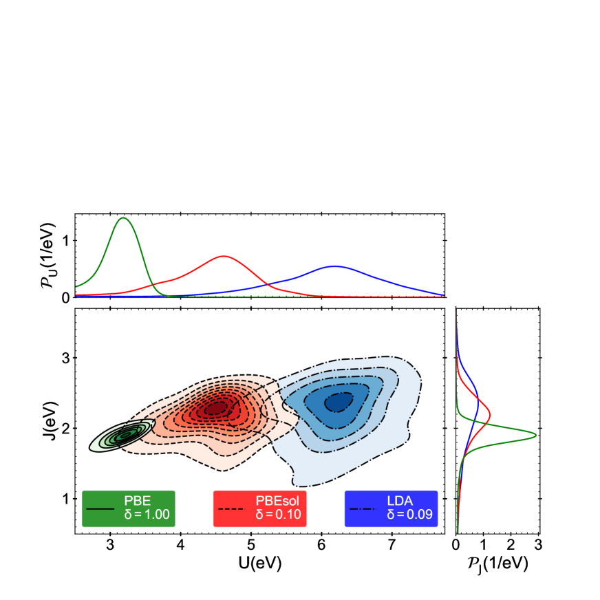
Figure 1: The density was estimated using a gaussian kernel density estimation (KDE). The bandwidth was selected using the Scott [97] approach. Each KDE is normalized to one separately. $\delta$ is the step between contour lines. (top left) Shows the probability density function of accepted $U$ parameters. (bottom left) Shows the joint probability density function of accepted $U$ and $J$. (bottom right) Shows the probability density function of accepted $J$ parameters.

The distribution of $U$ and $J$ parameters is more localized in PBE comparing to that of LDA and PBEsol. This can be visualized in Figure 1 by noting the spread of the distribution in the parameter space in each case. Furthermore, the univariate analysis, provided in Table 1, shows that PBE has a noticeably smaller overall standard deviation ($\sigma_{UJ}$) than LDA and PBEsol. A small overall standard deviation of $U$ and $J$ in the parameter space (i.e. a localized distribution) indicates that using the mean values $U_{avg}$ and $J_{avg}$ simultaneously improves the results toward a better agreement with the experimental data for all of the structures. Therefore, we expect $U_{avg}$ and $J_{avg}$ values from the distribution for PBE+$U$ are more transferable to other materials than LDA+$U$ and PBEsol+$U$.

The last column of Table 1 shows the Pearson correlation coefficient of the $U$ and $J$ parameter ($\rho_{UJ}$). If the correlation factor is equal to zero, $U$ and $J$ are completely independent. As the correlation approaches one, the dependence increases. If the correlation is equal to one, $U$ and $J$ are completely dependent. This is reminiscent of the Dudarev approximation  [98], a more simplified yet rotationally invariant form, where the functional can be obtained by only considering the zeroth-order Slater integral. The treatment of $U$ and $J$ values in Ref.  98 is analogous to incorporating the exchange interaction to the Coulomb interaction using an effective $U$, $U_{\mathrm{eff}}=U–J$  [95]. Within the Dudarev approximation the two parameters of Lichtenstein form, $U$ and $J$, are effectively reduced to one parameter, $U_{\mathrm{eff}}$. We find that PBE has the largest correlation between $U$ and $J$. This seems to indicate that out of the three studied XC functionals, PBE has the closest result between Dudarev approximation  [98] and Lichtenstein form [81].

We have recorded the experimental and predicted values of lattice parameters, volume, bandgap, and magnetic moment for the studied materials in Table 2. Even though volume, bandgap, and magnetic moment were set equally as target parameters, it can be seen that the corrections for lattice parameters have been more effective than the bandgap and magnetic moment. This is because treating the volume on the same footing as bandgap and magnetic moment increases the importance of the lattice parameters. Also, changes in lattice parameters can subsequently effect the magnetic moment and bandgap predictions.

Table 2: Structural, electronic, and magnetic properties of selected iron-based compounds. Values outside (inside) parenthesis are from simulations using DFT (DFT+$U$). The DFT+$U$ calculations were performed using the mean values of $U$ and $J$ from the distributions. Letters a, b, and c represent the lattice parameters. MP represents the final magnetic phase. Volume, bandgap, and magnetic moment are expressed in units of ų, eV, and Bohr magneton ($\mu_{B}$), respectively.

Material	XC	a	b	c	Volume	Bandgap	Mag. Mom.	MP
Fe	Experiment	2.87a			23.64	0.0b	2.22c	FMb
Im$\overline{3}$m	LDA (+$U$)	2.75 (2.83)			20.71 (22.55)	0.00 (0.00)	1.95 (2.73)	FM (FM)
	PBE, (+$U$)	2.83 (2.84)			22.58 (22.96)	0.00 (0.00)	2.19 (2.09)	FM (FM)
	PBEsol (+$U$)	2.78 (2.85)			21.59 (23.22)	0.00 (0.00)	2.12 (2.71)	FM (FM)
Fe2P	Experiment	5.87d		3.46d	119.34	0.0e	1.91f (Fe(II))	FMf
P$\overline{6}$2m	LDA +$U$)	5.56 (5.88)		3.42 (3.32)	91.31 (99.37)	0.00 (0.00)	1.11 (2.26)	FM (FM)
	PBE (+$U$)	5.81 (5.91)		3.41 (3.38)	99.55 (102.43)	0.00 (0.00)	2.25 (2.09)	FM (FM)
	PBEsol (+$U$)	5.70 (5.90)		3.40 (3.36)	95.70 (101.25)	0.00 (0.00)	2.03 (2.23)	FM (FM)
Fe3Ge	Experiment	5.17g		4.22g	112.79	0.0g	2.00g	FMg
P63/mmc	LDA (+$U$)	4.95 (5.18)		4.03 (4.17)	85.69 (96.80)	0.00 (0.00)	1.25 (2.75)	FM (FM)
	PBE (+$U$)	5.14 (5.17)		4.20 (4.21)	95.83 (97.50)	0.00 (0.00)	2.18 (2.37)	FM (FM)
	PBEsol (+$U$)	5.15 (5.17)		4.22 (4.28)	96.85 (98.97)	0.00 (0.00)	2.17 (2.66)	FM (FM)
BaFeO3	Experiment	3.97h			62.57	1.8i	3.50i	FMi
Pm$\overline{3}$m	LDA (+$U$)	3.86 (3.90)			57.31 (59.09)	0.00 (0.00)	2.64 (3.56)	FM (FM)
	PBE (+$U$)	3.97 (3.98)			62.47 (63.24)	0.00 (0.00)	3.02 (3.37)	FM (FM)
	PBEsol (+$U$)	3.90 (3.91)			59.39 (59.75)	0.00 (0.00)	2.88 (3.45)	FM (FM)
SrFeO3	Experiment	3.85j			57.06	1.8k	3.10m	FMo
Pm$\overline{3}$m	LDA (+$U$)	3.74 (3.78)			52.24 (53.93)	0.00 (0.00)	2.51 (3.49)	FM (FM)
	PBE (+$U$)	3.84 (3.85)			56.70 (57.21)	0.00 (0.00)	2.87 (3.15)	FM (FM)
	PBEsol (+$U$)	3.77 (3.79)			53.45 (54.64)	0.00 (0.00)	2.71 (3.36)	FM (FM)
FeO	Experiment	4.31q,s			80.06	1p-2.4r	3.32q	AFMq
Fm$\overline{3}$m	LDA (+$U$)	4.15 (4.20)			71.28 (73.31)	0.00 (2.85)	3.30 (0.12)	AFM (AFM)
	PBE (+$U$)	4.24 (4.27)			76.43 (77.74)	0.00 (0.00)	3.40 (3.51)	AFM (AFM)
	PBEsol (+$U$)	4.15 (4.22)			70.25 (75.24)	0.00 (0.00)	3.29 (3.55)	AFM (AFM)
$\alpha-$Fe2O3	Experiment	5.03t		13.75t	301.82	2.1u	4.9u	AFMv
R$\overline{3}$c	LDA (+$U$)	4.62 (4.95)		13.31 (13.60)	246.03 (289.03)	0.00 (1.74)	1.11 (4.00)	AFM (AFM)
	PBE, (+$U$)	5.00 (5.05)		13.86 (13.91)	300.59 (306.85)	0.53 (1.15)	3.55 (3.85)	AFM (AFM)
	PBEsol (+$U$)	4.91 (5.00)		13.66 (13.73)	285.18 (297.22)	0.30 (1.49)	3.36 (3.95)	AFM (AFM)
AlFeB2	Experiment	2.92w	11.03w	2.87w	92.23w	0.0x	1.21w,y,z	FMw,y,z
Cmmm	LDA (+$U$)	2.90 (2.87)	11.13 (10.84)	2.64 (2.85)	85.17 (88.53)	0.0 (0.0)	0.0 (1.64)	FM (FM)
	PBE (+$U$)	2.92 (2.92)	11.01 (11.01)	2.86 (2.86)	91.91 (91.91)	0.0 (0.0)	1.40 (1.52)	FM (FM)
	PBEsol (+$U$)	2.92 (2.92)	11.01 (11.01)	2.86 (2.86)	91.91 (91.91)	0.0 (0.0)	1.37 (1.57)	FM (FM)
Fe5PB2	Experiment	5.49l		10.35l	311.67	0.0	1.73 l	FMl
I4/mcm	LDA (+$U$)	5.45 (5.45)		10.31 (10.31)	306.45 (306.45)	0.0 (0.0)	1.43 (2.21)	FM (FM)
	PBE (+$U$)	5.44 (5.51)		10.34 (10.39)	305.79 (315.32)	0.0 (0.0)	1.79 (1.99)	FM (FM)
	PBEsol (+$U$)	5.35 (5.48)		10.18 (10.26)	292.08 (308.12)	0.0 (0.0)	1.55 (2.11)	FM (FM)
Fe5SiB2	Experiment	5.55l		10.34l	318.45	0.0	1.83l	FMl
I4/mcm	LDA (+$U$)	5.45 (5.45)		10.31 (10.31)	306.45 (306.45)	0.00 (0.0)	1.48 (2.11)	FM (FM)
	PBE (+$U$)	5.50 (5.54)		10.33 (10.42)	312.25 (320.29)	0.00 (0.0)	1.84 (1.98)	FM (FM)
	PBEsol (+$U$)	5.43 (5.51)		10.12 (10.27)	298.58 (312.42)	0.0 (0.0)	1.61 (2.04)	FM (FM)

^a Ref. 99; ^b Ref. 100; ^c Ref. 101; ^d Ref. 102; ^e Ref. 103; ^f Ref. 85; ^g Ref. 86; ^h Ref. 104; ⁱ Ref. 91; ^j Ref. 105; ^k Ref. 93; ^l Ref. 106; ^m Ref. 107; ⁿ Ref. 108; ^o Ref. 109; ^p Ref. 110; ^q Ref. 111; ^r Ref. 112; ^s Ref. 113; ^t Ref. 114; ^u Ref. 115; ^v Ref. 116; ^w Ref. 117; ^x Ref. 118; ^y Ref. 119; ^z Ref. 120.

We selected an accuracy criterion of 0.09 Å and compared the experimental and predicted lattice parameters before and after the Hubbard correction. As expected, LDA usually underestimates the lattice parameters. This corroborates our previous findings that LDA needs a larger $U$ value to correct the underestimation of the bond lengths. The introduction of the correction parameters improves the prediction for most of the structures. As mentioned before, PBE is known for overestimating lattice parameters in non-correlated materials. For strongly correlated materials, as in the case of this study, this trend benefits PBE in predicting the lattice parameters reasonably accurately without any corrections. This was also observed by Meng et al. [121] in their study of a group of iron oxides using beyond-DFT approaches, where they observed adding the suggested $U$ and $J$ parameters to PBE minimally influence the lattice parameters prediction. This result also supports our previous observation that PBE requires smaller correction parameters. On the other hand, PBEsol underestimates the lattice parameters. This was expected because PBEsol was introduced to correct the overestimation of PBE. The $U$ and $J$ parameters suggested in this study improve the lattice parameter prediction in PBEsol. Detailed analysis can be found in supplementary Table 2.

The same analysis was performed for the magnetic moment with an accuracy criterion of 0.2 $\mu_{B}$. Magnetic moment predictions by LDA are underestimated for all of the structures. This underestimation frequently turns to an overestimation by introducing the correctional parameters. PBE, however, usually predicts the magnetic moment accurately, and adding the suggested $U$ and $J$ does not change the number of accurate predictions. PBEsol, similar to LDA, underestimates the magnetic moment. The suggested correctional parameters convert this underestimation to overestimation. Detailed analysis can be found in supplementary Table 3.

As for bandgap predictions, predicting a zero bandgap by DFT+$U$ is not remarkable. The materials listed with a bandgap in Table 2 are BaFeO3, SrFeO3, FeO, and $\alpha$-Fe2O3.BaFeO3 exhibits a metallic behavior even after the Hubbard correction. Additional calculations were performed with the aim to open the bandgap in this compound using higher values of $U$. However, this was not achieved, even with values as high as 8 eV. Similarly, SrFeO3 also shows a metallic behavior with and without the correctional parameters. Experimentally it has both metallic and insulating phases [88]. To be able to capture the insulating phase using DFT one has to prepare a structure that includes both HM and FM domains. For FeO (wüstite), the only XC functional that could open a bandgap using the Hubbard correction was LDA, however, the magnetic moment was drastically underestimated. Prediction of the correct bandgap in FeO requires special care associated with the occupancies of the 3$d$ states [46]. Mandal et al. [122, 123] showed DFT+$U$ is not sufficient for reproducing the experimental results of FeO and one has to employ DFT+DMFT [29, 30, 31, 32, 33, 34, 35, 36, 37] method to accurately predict the AFM state of FeO. As for $\alpha$-Fe2O3 (hematite), before introducing $U$ and $J$ parameters, LDA predicted a metallic behavior, while PBE and PBEsol opened a small bandgap. Using the correctional parameters all three XC functionals estimated an acceptable bandgap without compromising other properties.

Finally, we show the root mean square error (RMSE) and mean absolute error (MAE) of the predicted properties (volume, magnetic moment) in Supplementary Table 4. The RMSE and MAE show the improvement in the predicted values in all of the XC functionals after including the Hubbard correction.

In summary, we selected a group of iron-based compounds and explored the space of the correction parameters $U$ and $J$ that can improve the prediction results (volume, magnetic moment, and bandgap) for all of the studied materials simultaneously. This semi-empirical exploration was done using a Bayesian calibration, assisted by Markov Chain Monte Carlo sampling. For these iron-based compounds, we extracted three sets of $U$ and $J$ for LDA, PBE, and PBEsol XC functionals. All the $U$ and $J$ distributions have a single maximum. LDA requires a significantly larger $U$ parameter comparing to GGA functionals. $U$ and $J$ achieved in PBE are the most transferable between the studied iron-based compounds. The Dudarev approximation can result in a closer prediction to the Lichtenstein form of the Hubbard interaction in PBE compared to that of LDA and PBEsol. Assessing the correction parameters obtained from the distributions, showed the suggested correctional parameters improve the prediction of the lattice parameters and the magnetic moment in all XC functionals. A correct bandgap was not predicted for FeO or BaFeO3, due to the inability of DFT+$U$ to reproduce the experimental results. In the case of $\alpha-$Fe2O3, bandgap estimation was improved for all the XC functionals. PBE predicts the lattice parameters reasonably accurately even without the Hubbard correction for these iron-based compounds. Lastly, based on the analysis performed in this study, we conclude that the $U$ and $J$ pairs provided can be a good starting point for DFT+$U$ calculations on the iron-based compound. In the future, it will be interesting to expand the parameter space to incorporate the details of the orbital occupation [58, 59, 60], the inter-site Hubbard $V$ [95], and pseudopotentials [124]. Moreover, various other properties such as cohesive energy, formation energy, elastic constants, etc. can be used in the dataset $X$. The proposed methodology can be employed for other systems to predict their properties for a given set of parameters within the spirit of high-throughput calculations.

3 Methods

3.1 DFT+$U$ and Bayesian calibration interface

Since the underlying model is nonlinear and the evidence $P(X)$ is intractable, we used MCMC to draw the samples from the distribution. The MCMC sampler used an adaptive block proposal. For each run of the sampler, post equilibration (burn-in) convergence was assessed using a standard of $\pm$ 5% for both $U$ and $J$ at 95% confidence using a Student t-test on batch means. Mixing of the sampler depicts a stationary behavior, and convergence was obtained for all runs after approximately 2000 post-burn-in draws.

This experiment is a set of back and forth communications between the DFT package and the MCMC sampler. The DFT+$U$ calculation is performed using the $U$ and $J$ parameters proposed by the MCMC sampler. Based on the accuracy of the DFT prediction in comparison with the experimental values, the MCMC sampler proposes a new pair of parameters drawn from a normal distribution centered at the $U$ and $J$ of the previous step for a new trial, and so on. We use a block-proposal scheme (both i.e. $U$ and $J$ are proposed at once). Our implementation uses an adaptive proposal where the covariance of the multivariate normal proposal distribution is shaped to the accepted points. At each MCMC step the likelihood is calculated and the proposal is accepted or rejected based on the Metropolis-Hastings algorithm (for more details see Ref.  66. A schematic representation of the algorithm is shown in Figure 2.

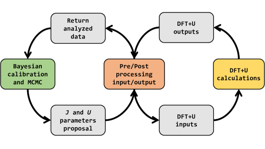
Figure 2: Computational process.

3.2 Computational details

The DFT calculations were performed using the Vienna Ab initio Simulation Package (VASP) [125, 126, 127, 128]. The valence electrons wave functions were described by the projector augmented-wave [129, 130] method. The kinetic energy expansion and optimum irreducible Brillouin zone grid (k-grid) for each structure were obtained by choosing a maximum error of 1 meV/atom for the total energy in each cell. We used $\Gamma$-centered and Monkhorst-Pack type [131] k-grids for hexagonal and cubic structures, respectively. Detailed convergence parameters are provided in supplementary Table 1. The Slater integrals values for Fe 3d shell were evaluated using the $U$, $J$, and the ratio of $F^{4}/F^{2}$, as implemented in VASP [132].

The Kohn-Sham equations were solved self-consistently with a maximum total energy difference of $10^{-5}$ eV. Furthermore, we assumed the crystal structure geometry to be optimized when the internal stress tensor components differ from the ambient pressure (assumed to be zero) by less than 0.5 kbar, and the residual forces on each atom are less than 1 meV/Å.

As a consequence of the MCMC random walk, the algorithm might step in unphysical areas of the parameter space where $J>U$. These values are expected to be proposed because the Markov chain is free to explore every possible region seeking points where the predictions are close to the provided experimental values. Initially, the algorithm has little guidance from past proposed parameters leading to the proposition of unphysical parameters. To penalize the MCMC walker anytime an unphysical pair is proposed by the sampler, we skip the DFT calculation and return senseless values for the DFT+$U$ prediction (e.g. bandgap = -50 eV, volume = -50 ų, magnetic moment = -50 $\mu_{B}$). This encourages the algorithm to avoid proposing unnatural parameters and to explore other areas of the parameter space. The same strategy is used to penalize the algorithm when the $U$ and $J$ correction results in a change of space group.

Supplementary information

Supplementary Table  4 shows the improvement in volume and magnetic moment prediction using DFT+$U$.

In Supplementary Table  5 for BaFe2As2 we used the Fmmm space group and started the computation with ferromagnetic (FM), stripe antiferromagnetic (s-AFM), and checkerboard antiferromagnetic (c-AFM) initial magnetic phases. The DFT+$U$ calculations were performed using the mean values of $U$ and $J$ from the distributions. This material was selected to evaluate the performance of these suggested $U$ and $J$ values in an iron-based superconductor. It is known that this compound is an antiferromagnet below approximately 140 K. LDA, regardless of XC functional, predicts a nonmagnetic (NM) phase. The total energies using LDA for the different magnetic phases are very similar to each other and do not allow an accurate prediction of the ground state. LDA+$U$ predicts the ground state of this compound to be s-AFM with a magnetic moment of 2.94 $\mu_{B}$. PBE predicts the s-AFM phase to be the most stable magnetic phase with a magnetic moment of 1.43 $\mu_{B}$, and PBE+$U$ predicts the FM phase as the ground state with an overestimated magnetic moment of 2.17 $\mu_{B}$. This example clearly demonstrates that certain materials require a larger $J$ value in order to accurately describe their magnetic behavior. For this specific compound, it appears preferable not to use the Hubbard correction than to use a small $J$ value. Lastly, PBEsol predicts the ground state to be s-AFM for both PBEsol and PBEsol+$U$. Similar to other XC functionals, the Hubbard correction tends to overestimate the magnetic moment (2.86 $\mu_{B}$) while the plain calculation better approaches the experimental values. As shown by Derondeau et al., calculations for this material often overestimate magnetic moments[137].

Supplementary Figure  2 shows percentage error heat maps of $U$ and $J$ for Fe and SrFeO3 for volume, bandgap, and magnetic moment predictions. The $U$ and $J$ pairs that provide the most accurate results are different for iron in different environments. The same can be said for the prediction of different properties in the same material, i.e. the $U$ and $J$ pairs that produce the closes result for volume are not the same for magnetic moment. For simplicity, here we show all prediction errors only for Fe and SrFeO3 in LDA+$U$. As plotted, we only show the pixels that were explored by the sampler. The $U$ and $J$ extracted from this sampling are shown as solid round magenta dots.

To evaluate the importance of target properties and the functionality of the method, we performed the experiment by omitting the bandgap from the target properties for LDA and PBE. This pushes the algorithm towards providing $U$ and $J$ pairs that improve the magnetic moment and the volume more than when bandgap is included in the target properties. The $U$ and $J$ parameters extracted from this sampling are provided in Supplementary Table  6. The probability distribution for sampling is shown in Supplementary Figure  3. Supplementary Table  7 shows the root mean square error (RMSE) and mean absolute error (MAE) from the DFT+$U$ calculation using the $U$ and $J$ pair extracted from this sampling.

The observation error variance $\phi$ is estimated during the calibration. $\phi$ has an Inverse Gamma distribution ($IG)$ prior  [66]. In principle, the $IG$ should be based on an a priori assessment of error in the experiment. We have generated these $IG$ by considering the mode and the mean to be twice and four times as large as the largest standard deviation of the target parameters, respectively. The standard deviations used for bandgap, magnetic moment, and volume were 0.01 eV, 0.01 $\AA^{3}$, and 0.1 $\mu_{B}$ respectively. This results in $\phi_{E_{g}}\sim IG(3,0.08)$, $\phi_{V}\sim IG(3,0.08)$, and $\phi_{\mu}\sim IG(3,0.8)$.

Supplementary Table 1: Convergence parameters. k-grid shows the dimension of the selected grid for the Brillouin zone. E_cut shows the cutoff of plane-wave expansion cutoff and it is presented in $eV$.

Material	LDA		PBE		PBEsol
	k-grid	Ecut	k-grid	Ecut	k-grid	Ecut
Fe	9$\times$9$\times$9	450	9$\times$9$\times$9	500	8$\times$8$\times$8	550
Fe2P	3$\times$3$\times$4	400	3$\times$3$\times$4	500	3$\times$3$\times$4	500
Fe3Ge	3$\times$3$\times$4	450	3$\times$3$\times$4	500	3$\times$3$\times$4	500
SrFeO3	8$\times$8$\times$8	900	8$\times$8$\times$8	900	8$\times$8$\times$8	900
BaFeO3	8$\times$8$\times$8	900	8$\times$8$\times$8	950	8$\times$8$\times$8	900

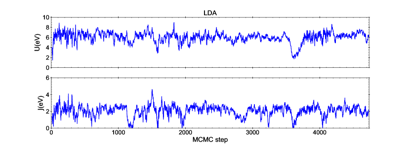
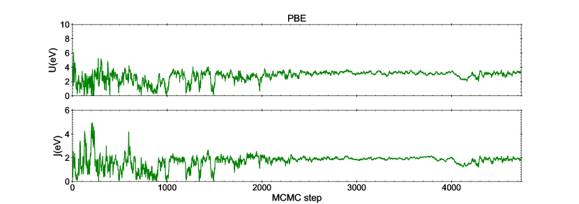
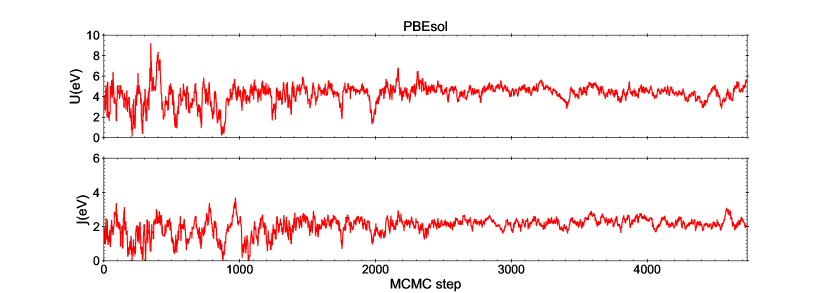
Supplementary Figure 1: Trace of MCMC algorithm for LDA, PBE, and PBEsol XC functionals.

Supplementary Table 2: Lattice parameter prediction evaluation for each XC functional and their corresponding Hubbard correction. Red, green, and white backgrounds depict underestimation, overestimation, and accurate, respectively. The accuracy criterion is 0.09 Å. $\Delta$ represents the prediction error.

Material	Parameter	Exp.	LDA	LDA+$U$	PBE	PBE+$U$	PBEsol	PBEsol+$U$	$\Delta_{LDA}$	$\Delta_{LDA+U}$	$\Delta_{PBE}$	$\Delta_{PBE+U}$	$\Delta_{PBEsol}$	$\Delta_{PBEsol+U}$
Fe	a	2.87	2.75	2.83	2.83	2.84	2.78	2.85	[HTML]FFC7CE -0.12	-0.04	-0.04	-0.03	[HTML]FFC7CE -0.09	-0.02
Fe2P	a	5.87	5.56	5.88	5.81	5.91	5.70	5.90	[HTML]FFC7CE -0.31	0.01	-0.06	0.04	[HTML]FFC7CE -0.17	0.03
Fe3Ge	a	5.17	4.95	5.18	5.14	5.17	5.15	5.17	[HTML]FFC7CE -0.22	0.01	-0.03	0.00	-0.02	0.00
BaFeO3	a	3.97	3.86	3.90	3.97	3.98	3.90	3.91	[HTML]FFC7CE -0.11	-0.07	0.00	0.01	-0.07	-0.06
SrFeO3	a	3.85	3.74	3.78	3.84	3.85	3.77	3.79	[HTML]FFC7CE -0.11	-0.07	-0.01	0.00	-0.08	-0.06
FeO	a	4.31	4.15	4.20	4.24	4.27	4.15	4.22	[HTML]FFC7CE -0.16	[HTML]FFC7CE -0.11	-0.07	-0.04	[HTML]FFC7CE -0.16	[HTML]FFC7CE -0.09
$\alpha$-Fe2O3	a	5.03	4.62	4.95	5.00	5.05	4.91	5.00	[HTML]FFC7CE -0.41	-0.08	-0.03	0.02	[HTML]FFC7CE -0.12	-0.03
AlFeB2	a	2.92	2.90	2.87	2.92	2.92	2.92	2.92	-0.02	-0.05	0.00	0.00	0.00	0.00
Fe5PB2	a	5.49	5.45	5.45	5.44	5.51	5.35	5.48	-0.04	-0.04	-0.05	0.02	[HTML]FFC7CE -0.14	-0.01
Fe5SiB2	a	5.55	5.45	5.45	5.50	5.54	5.43	5.51	[HTML]FFC7CE -0.10	[HTML]FFC7CE -0.10	-0.05	-0.01	[HTML]FFC7CE -0.12	-0.04
AlFeB2	b	11.03	11.13	10.84	11.01	11.01	11.01	11.01	[HTML]C6EFCE 0.10	[HTML]FFC7CE -0.19	-0.02	-0.02	-0.02	-0.02
Fe2P	c	3.46	3.42	3.32	3.41	3.38	3.40	3.36	-0.04	[HTML]FFC7CE -0.14	-0.05	-0.08	-0.06	[HTML]FFC7CE -0.10
Fe3Ge	c	4.22	4.03	4.17	4.20	4.21	4.22	4.28	[HTML]FFC7CE -0.19	-0.05	-0.02	-0.01	0.00	0.06
$\alpha$-Fe2O3	c	13.75	13.31	13.60	13.86	13.91	13.66	13.73	[HTML]FFC7CE -0.44	[HTML]FFC7CE -0.15	[HTML]C6EFCE 0.11	[HTML]C6EFCE 0.16	[HTML]FFC7CE -0.09	-0.02
AlFeB2	c	2.87	2.64	2.85	2.86	2.86	2.86	2.86	[HTML]FFC7CE -0.23	-0.02	-0.01	-0.01	-0.01	-0.01
Fe5PB2	c	10.35	10.31	10.31	10.34	10.39	10.18	10.26	-0.04	-0.04	-0.01	0.04	[HTML]FFC7CE -0.17	[HTML]FFC7CE -0.09
Fe5SiB2	c	10.34	10.31	10.31	10.33	10.42	10.12	10.27	-0.03	-0.03	-0.01	0.08	[HTML]FFC7CE -0.22	-0.07

Supplementary Table 3: Magnetic moment prediction evaluation for each XC functional and their corresponding Hubbard correction. Red, green, and white backgrounds depict underestimation, overestimation, and accurate, respectively. The accuracy criterion is 0.2 $\mu_{B}$. $\Delta$ represents the prediction error.

[HTML]FFFFFF Material	Exp.	LDA	LDA+$U$	PBE	PBE+$U$	PBEsol	PBEsol+$U$	$\Delta_{LDA}$	$\Delta_{LDA+U}$	$\Delta_{PBE}$	$\Delta_{PBE+U}$	$\Delta_{PBEsol}$	$\Delta_{PBEsol+U}$
Fe	2.22	1.95	2.73	2.19	2.09	2.12	2.71	[HTML]FFC7CE -0.27	[HTML]C6EFCE 0.51	-0.03	-0.13	[HTML]FFC7CE -0.10	[HTML]C6EFCE 0.49
Fe2P	1.91	1.11	2.26	2.25	2.09	2.03	2.23	[HTML]FFC7CE -0.80	[HTML]C6EFCE 0.35	[HTML]C6EFCE 0.34	0.18	[HTML]FFC7CE 0.12	[HTML]C6EFCE 0.32
Fe3Ge	2.00	1.25	2.75	2.18	2.37	2.17	2.66	[HTML]FFC7CE -0.75	[HTML]C6EFCE 0.75	0.18	[HTML]C6EFCE 0.37	0.17	[HTML]C6EFCE 0.66
BaFeO3	3.50	2.64	3.56	3.02	3.37	2.88	3.45	[HTML]FFC7CE -0.86	0.06	[HTML]FFC7CE -0.48	-0.13	[HTML]FFC7CE -0.62	-0.05
SrFeO3	3.10	2.51	3.49	2.87	3.15	2.71	3.36	[HTML]FFC7CE -0.59	[HTML]C6EFCE 0.39	[HTML]FFC7CE -0.23	0.05	[HTML]FFC7CE -0.39	[HTML]C6EFCE 0.26
FeO	3.32	3.30	0.12	3.40	3.51	3.29	3.55	[HTML]FFC7CE -0.02	[HTML]FFC7CE -3.20	0.08	0.19	[HTML]FFC7CE -0.03	[HTML]C6EFCE 0.23
$\alpha$-Fe2O3	4.90	1.11	4.00	3.55	3.85	3.36	3.95	[HTML]FFC7CE -3.79	[HTML]FFC7CE -0.90	[HTML]FFC7CE -1.35	[HTML]FFC7CE -1.05	[HTML]FFC7CE -1.54	[HTML]FFC7CE -0.95
AlFeB2	1.21	0.00	1.64	1.40	1.52	1.37	1.57	[HTML]FFC7CE -1.21	[HTML]C6EFCE 0.43	0.19	[HTML]C6EFCE 0.31	0.16	[HTML]C6EFCE 0.36
Fe5PB2	1.73	1.43	2.21	1.79	1.99	1.55	2.11	[HTML]FFC7CE -0.30	[HTML]C6EFCE 0.48	0.06	[HTML]C6EFCE 0.26	[HTML]FFC7CE -0.18	[HTML]C6EFCE 0.38
Fe5SiB2	1.83	1.48	2.11	1.84	1.98	1.61	2.04	[HTML]FFC7CE -0.35	[HTML]C6EFCE 0.28	0.01	0.15	[HTML]FFC7CE -0.22	[HTML]C6EFCE 0.21

Supplementary Table 4: Root mean square error (RMSE) and mean absolute error (MAE) for prediction using DFT and DFT+$U$. Note, after including the Hubbard correction, predictions for volume and magnetic moment ($V$ and $\mu$) improve. Green represents improvement in predictions.

	Target Property	LDA	LDA+$U$	PBE	PBE+$U$	PBEsol	PBEsol+$U$	DFT	DFT+$U$
RSME	Volume $(\AA^{3})$	22.34	[HTML]C6EFCE 10.50	8.77	[HTML]C6EFCE 7.54	14.11	[HTML]C6EFCE7.91	16.07	[HTML]C6EFCE 8.75
	Mag. Mom. $(\mu_{B})$	1.36	[HTML]C6EFCE 1.12	0.48	[HTML]C6EFCE 0.39	0.55	[HTML]C6EFCE 0.46	0.89	[HTML]C6EFCE 0.74
MAE	Volume $(\AA^{3})$	15.70	[HTML]C6EFCE 8.61	5.55	[HTML]C6EFCE 4.69	11.47	[HTML]C6EFCE 5.69	10.91	[HTML]C6EFCE 6.33
	Mag. Mom. $(\mu_{B})$	0.89	[HTML]C6EFCE 0.74	0.30	[HTML]C6EFCE 0.28	0.35	[HTML]C6EFCE 0.39	0.51	[HTML]C6EFCE 0.47

Supplementary Table 5: Structural, electronic, and magnetic properties of BaFe2As2. Values outside (inside) parenthesis are from simulations using DFT (DFT+$U$). The DFT+$U$ calculations were performed using the mean values of $U$ and $J$ from the distributions. Letters a, b, and c represent the lattice parameters. MP represents the final magnetic phase. Volume and magnetic moment are expressed in units of ų and Bohr magneton ($\mu_{B}$), respectively.

Material	XC	a	b	c	Volume	Mag. Mom.	MP
BaFe2As2	Experiment	5.61 a	5.57 a	12.95 a	405.14 a	0.40, 0.5, 0.87 a,b,c	AFM a
Ferromagnet	LDA (+$U$)	5.48 (5.54)	5.48 (5.54)	12.30 (13.32)	369.52 (408.79)	0.00 (1.74)	NM (FM)
	PBE (+$U$)	5.60 (5.64)	5.60 (5.63)	12.60 (13.49)	395.86 (427.83)	0.00 (1.43)	NM (FM)
	PBEsol (+$U$)	5.53 (5.56)	5.53 (5.55)	12.34 (13.37)	377.35 (411.56)	0.00 (1.56)	NM (FM)
Antiferromagnet	LDA (+$U$)	5.48 (5.82)	5.48 (5.40)	12.30 (13.19)	369.50 (415.03)	0.00 (2.89)	NM (AFM)
stripe	PBE (+$U$)	5.68 (5.93)	5.58 (5.58)	12.88 (13.16)	408.39 (435.75)	1.90 (2.73)	AFM (AFM)
	PBEsol (+$U$)	5.54 (5.85)	5.54 (5.85)	12.65 (13.09)	380.99 (420.13)	1.11 (2.86)	AFM (AFM)
Antiferromagnet	LDA (+$U$)	5.48 (5.88)	5.48 (5.29)	12.30 (13.42)	369.53 (417.64)	0.00 (2.50)	NM (AFM)
checkerboard	PBE (+$U$)	5.63 (6.01)	5.63 (5.47)	12.70 (13.36)	403.05 (439.60)	1.38 (2.17)	AFM (AFM)
	PBEsol (+$U$)	5.53 (5.91)	5.53 (5.35)	12.34 (13.36)	377.36 (422.91)	0.00 (2.39)	NM (AFM)

^a Ref.  138; ^b Ref.  139; ^c Ref.  140;

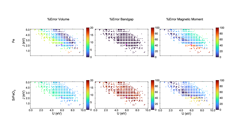
Supplementary Figure 2: LDA+$U$ prediction percentage error heat maps of $U$ and $J$ for Fe and SrFeO3 for volume, bandgap, and magnetic moment.

Supplementary Table 6: $U$ and $J$ values extracted from MCMC sampling with and without bandgap as a target parameter. $\mu$, V, and $E_{g}$ represent magnetic moment, volume, and bandgap, respectively.

XC	LDA+$U$	LDA+$U$	PBE+$U$	PBE+$U$
Target properties	$\mu$, $V$, $E_{g}$	$\mu$, $V$	$\mu$, $V$, $E_{g}$	$\mu$, $V$
$U$ (eV)	5.9	6.4	3.1	3.1
$J$ (eV)	2.1	1.9	1.9	1.8

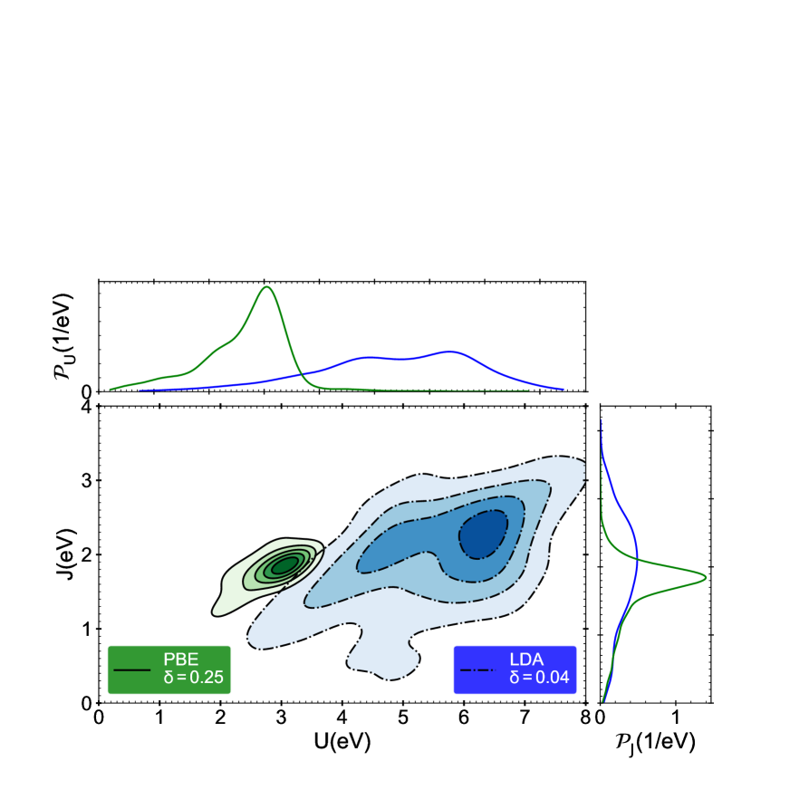
Supplementary Figure 3: $U$ and $J$ values extracted from MCMC sampling without bandgap in the target properties. Target properties in this sampling are volume and magnetic moment. The density was estimated using a gaussian kernel density estimation (KDE). The bandwidth was selected using the Scott approach. Each KDE is separately normalized to one. $\delta$ is the step between contour lines. Top left shows the probability density function of accepted $U$ parameters. Bottom left shows the joint probability density function of accepted $U$ and $J$. Bottom right shows the probability density function of accepted $J$ parameters.

Supplementary Table 7: RMSE and MAE of DFT+$U$ with $U$ and $J$ values extracted from MCMC samplings with and without bandgap included in the target parameters.

	RMSE	RMSE	MAE	MAE
Target properties	$\mu$, $V$, $E_{g}$	$\mu$, $V$	$\mu$, $V$, $E_{g}$	$\mu$, $V$
Volume ($\AA^{3}$)	8.75	[HTML]C6EFCE6.68	6.33	[HTML]C6EFCE3.98
Mag. Mom. ($\mu_{B}$)	0.74	[HTML]C6EFCE0.39	0.47	[HTML]C6EFCE0.26

References

- [1] Hohenberg, P. & Kohn, W. Inhomogeneous Electron Gas. Phys. Rev. 136, B864–B871 (1964). URL https://link.aps.org/doi/10.1103/PhysRev.136.B864.
- [2] Kohn, W. & Sham, L. J. Self-Consistent Equations Including Exchange and Correlation Effects. Phys. Rev. 140, A1133–A1138 (1965). URL https://link.aps.org/doi/10.1103/PhysRev.140.A1133.
- [3] Kohn, W., Becke, A. D. & Parr, R. G. Density Functional Theory of Electronic Structure. J. Phys. Chem. 100, 12974–12980 (1996). URL https://doi.org/10.1021/jp960669l.
- [4] Steckel, J. A. & Sholl, D. Density Functional Theory (John Wiley & Sons, Ltd, Hoboken, 2009). URL https://onlinelibrary.wiley.com/doi/abs/10.1002/9780470447710.
- [5] Fiolhais, C., Nogueira, F. & Marques, M. A. A primer in density functional theory, vol. 620 (Springer Berlin Heidelberg, Berlin Heidelberg, 2003). URL https://doi.org/10.1007/3-540-37072-2.
- [6] Parr, R. G. Density Functional Theory of Atoms and Molecules. In Fukui, K. & Pullman, B. (eds.) Horizons of Quantum Chemistry, 5–15 (Springer, Dordrecht, 1980).
- [7] Becke, A. D. Density-functional exchange-energy approximation with correct asymptotic behavior. Phys. Rev. A 38, 3098–3100 (1988). URL https://link.aps.org/doi/10.1103/PhysRevA.38.3098.
- [8] Perdew, J. P. et al. Atoms, molecules, solids, and surfaces: Applications of the generalized gradient approximation for exchange and correlation. Phys. Rev. B 46, 6671–6687 (1992). URL https://link.aps.org/doi/10.1103/PhysRevB.46.6671.
- [9] Lee, C., Yang, W. & Parr, R. G. Development of the Colle-Salvetti correlation-energy formula into a functional of the electron density. Phys. Rev. B 37, 785–789 (1988). URL https://link.aps.org/doi/10.1103/PhysRevB.37.785.
- [10] Perdew, J. P., Burke, K. & Wang, Y. Generalized gradient approximation for the exchange-correlation hole of a many-electron system. Phys. Rev. B 54, 16533–16539 (1996). URL https://link.aps.org/doi/10.1103/PhysRevB.54.16533.
- [11] Csonka, G. I. et al. Assessing the performance of recent density functionals for bulk solids. Phys. Rev. B 79, 155107 (2009). URL https://link.aps.org/doi/10.1103/PhysRevB.79.155107.
- [12] Sun, J., Ruzsinszky, A. & Perdew, J. P. Strongly Constrained and Appropriately Normed Semilocal Density Functional. Phys. Rev. Lett. 115, 036402 (2015). URL https://link.aps.org/doi/10.1103/PhysRevLett.115.036402.
- [13] Kim, K. & Jordan, K. Comparison of density functional and MP2 calculations on the water monomer and dimer. J. Phys. Chem. 98, 10089–10094 (1994). URL https://doi.org/10.1021/j100091a024.
- [14] Sun, J., Xiao, B. & Ruzsinszky, A. Communication: Effect of the orbital-overlap dependence in the meta generalized gradient approximation. J. Chem. Phys. 137, 051101 (2012). URL https://doi.org/10.1063/1.4742312.
- [15] Scuseria, G. E. & Staroverov, V. N. Chapter 24 - Progress in the development of exchange-correlation functionals. In Dykstra, C. E., Frenking, G., Kim, K. S. & Scuseria, G. E. (eds.) Theory and Applications of Computational Chemistry, 669–724 (Elsevier, Amsterdam, 2005). URL https://www.sciencedirect.com/science/article/pii/B9780444517197500676.
- [16] Mardirossian, N. & Head-Gordon, M. Thirty years of density functional theory in computational chemistry: an overview and extensive assessment of 200 density functionals. Mol. Phys. 115, 2315–2372 (2017). URL https://doi.org/10.1080/00268976.2017.1333644.
- [17] Misra, P. K. Chapter 7 - Electron–Electron Interaction. In Misra, P. K. (ed.) Physics of Condensed Matter, 199–242 (Academic Press, Boston, 2012). URL http://www.sciencedirect.com/science/article/pii/B9780123849540000074.
- [18] Heyd, J., Peralta, J. E., Scuseria, G. E. & Martin, R. L. Energy band gaps and lattice parameters evaluated with the Heyd-Scuseria-Ernzerhof screened hybrid functional. J. Chem. Phys. 123, 174101 (2005). URL https://doi.org/10.1063/1.2085170.
- [19] Verma, P. & Truhlar, D. G. HLE16: A Local Kohn–Sham Gradient Approximation with Good Performance for Semiconductor Band Gaps and Molecular Excitation Energies. J. Phys. Chem. Lett. 8, 380–387 (2017). URL https://doi.org/10.1021/acs.jpclett.6b02757.
- [20] Arbuznikov, A. V. Hybrid exchange correlation functionals and potentials: Concept elaboration. J. Struct. Chem. 48, S1–S31 (2007). URL https://doi.org/10.1007/s10947-007-0147-0.
- [21] Perdew, J. P., Ernzerhof, M. & Burke, K. Rationale for mixing exact exchange with density functional approximations. J. Chem. Phys. 105, 9982–9985 (1996). URL https://doi.org/10.1063/1.472933.
- [22] Becke, A. D. A new mixing of Hartree–Fock and local density‐functional theories. J. Chem. Phys. 98, 1372–1377 (1993). URL https://doi.org/10.1063/1.464304.
- [23] Heyd, J., Scuseria, G. E. & Ernzerhof, M. Hybrid functionals based on a screened Coulomb potential. J. Chem. Phys. 118, 8207–8215 (2003). URL https://doi.org/10.1063/1.1564060.
- [24] Georges, A., Kotliar, G., Krauth, W. & Rozenberg, M. J. Dynamical mean-field theory of strongly correlated fermion systems and the limit of infinite dimensions. Rev. Mod. Phys. 68, 13–125 (1996). URL https://link.aps.org/doi/10.1103/RevModPhys.68.13.
- [25] Georges, A. & Kotliar, G. Hubbard model in infinite dimensions. Phys. Rev. B 45, 6479–6483 (1992). URL https://link.aps.org/doi/10.1103/PhysRevB.45.6479.
- [26] Kotliar, G. & Vollhardt, D. Strongly correlated materials: Insights from dynamical mean-field theory. Phys. Today 57, 53–60 (2004). URL https://doi.org/10.1063/1.1712502.
- [27] Kotliar, G. et al. Electronic structure calculations with dynamical mean-field theory. Rev. Mod. Phys. 78, 865–951 (2006). URL https://link.aps.org/doi/10.1103/RevModPhys.78.865.
- [28] Georges, A. Strongly Correlated Electron Materials: Dynamical Mean‐Field Theory and Electronic Structure. AIP Conf. Proc. 715, 3–74 (2004). URL https://aip.scitation.org/doi/abs/10.1063/1.1800733.
- [29] Vollhardt, D., Byczuk, K. & Kollar, M. Dynamical Mean-Field Theory, 203–236 (Springer Berlin Heidelberg, Berlin, Heidelberg, 2012). URL https://doi.org/10.1007/978-3-642-21831-6_7.
- [30] DMFTwDFT: An open-source code combining Dynamical Mean Field Theory with various density functional theory packages. Comput. Phys. Commun. 261, 107778 (2021). URL http://www.sciencedirect.com/science/article/pii/S001046552030388X.
- [31] Paul, A. & Birol, T. Applications of DFT + DMFT in Materials Science. Annu. Rev. Mater. Res. 49, 31–52 (2019). URL https://doi.org/10.1146/annurev-matsci-070218-121825.
- [32] Kent, P. R. & Kotliar, G. Toward a predictive theory of correlated materials. Science 361, 348–354 (2018). URL https://www.science.org/doi/abs/10.1126/science.aat5975.
- [33] Haule, K. & Birol, T. Free energy from stationary implementation of the DFT+ DMFT functional. Phys. Rev. Lett. 115, 256402 (2015). URL https://link.aps.org/doi/10.1103/PhysRevLett.115.256402.
- [34] Haule, K. Exact double counting in combining the dynamical mean field theory and the density functional theory. Phys. Rev. Lett. 115, 196403 (2015). URL https://link.aps.org/doi/10.1103/PhysRevLett.115.196403.
- [35] Koçer, C. P., Haule, K., Pascut, G. L. & Monserrat, B. Efficient lattice dynamics calculations for correlated materials with DFT+ DMFT. Phys. Rev. B 102, 245104 (2020). URL https://link.aps.org/doi/10.1103/PhysRevB.102.245104.
- [36] Aichhorn, M. et al. TRIQS/DFTTools: A TRIQS application for ab initio calculations of correlated materials. Comput. Phys. Commun. 204, 200–208 (2016). URL https://www.sciencedirect.com/science/article/pii/S0010465516300728.
- [37] Vollhardt, D., Anisimov, V., Skornyakov, S. & Leonov, I. Dynamical mean-field theory for correlated electron materials. Mater. Today: Proc. 14, 176–180 (2019). URL https://www.sciencedirect.com/science/article/pii/S2214785319309022.
- [38] Himmetoglu, B., Floris, A., de Gironcoli, S. & Cococcioni, M. Hubbard-corrected DFT energy functionals: The LDA+ description of correlated systems. Int. J. Quantum Chem. 114, 14–49 (2014). URL https://onlinelibrary.wiley.com/doi/abs/10.1002/qua.24521.
- [39] Anisimov, V. I., Aryasetiawan, F. & Lichtenstein, A. I. First-principles calculations of the electronic structure and spectra of strongly correlated systems: the LDA+ method. J. Condens. Matter Phys. 9, 767–808 (1997). URL https://doi.org/10.1088/0953-8984/9/4/002.
- [40] Hubbard, J. & Flowers, B. H. Electron correlations in narrow energy bands. Proc. R. Soc. A 276, 238–257 (1963). URL https://royalsocietypublishing.org/doi/abs/10.1098/rspa.1963.0204.
- [41] Hubbard, J. & Flowers, B. H. Electron Correlations in Narrow Energy Bands. III. An Improved Solution. Proc. R. Soc. A 281, 401–419 (1964). URL https://royalsocietypublishing.org/doi/abs/10.1098/rspa.1964.0190.
- [42] Anisimov, V. I. (ed.) Strong Coulomb Correlations in Electronic Structure Calculations (CRC Press, London, 2000). URL https://doi.org/10.1201/9781482296877.
- [43] Anisimov, V. I., Aryasetiawan, F. & Lichtenstein, A. First-principles calculations of the electronic structure and spectra of strongly correlated systems: the LDA+ method. J. Condens. Matter Phys. 9, 767–808 (1997). URL https://doi.org/10.1088/0953-8984/9/4/002.
- [44] Wang, L., Maxisch, T. & Ceder, G. Oxidation energies of transition metal oxides within the GGA+ framework. Phys. Rev. B 73, 195107 (2006). URL https://link.aps.org/doi/10.1103/PhysRevB.73.195107.
- [45] Pickett, W. E., Erwin, S. C. & Ethridge, E. C. Reformulation of the LDA+ method for a local-orbital basis. Phys. Rev. B 58, 1201–1209 (1998). URL https://link.aps.org/doi/10.1103/PhysRevB.58.1201.
- [46] Cococcioni, M. & de Gironcoli, S. Linear response approach to the calculation of the effective interaction parameters in the LDA+ method. Phys. Rev. B 71, 035105 (2005). URL https://link.aps.org/doi/10.1103/PhysRevB.71.035105.
- [47] Aryasetiawan, F., Karlsson, K., Jepsen, O. & Schönberger, U. Calculations of Hubbard from first-principles. Phys. Rev. B 74, 125106 (2006). URL https://link.aps.org/doi/10.1103/PhysRevB.74.125106.
- [48] Timrov, I., Marzari, N. & Cococcioni, M. Hubbard parameters from density-functional perturbation theory. Phys. Rev. B 98, 085127 (2018). URL https://link.aps.org/doi/10.1103/PhysRevB.98.085127.
- [49] Timrov, I., Marzari, N. & Cococcioni, M. Self-consistent Hubbard parameters from density-functional perturbation theory in the ultrasoft and projector-augmented wave formulations. Phys. Rev. B 103, 045141 (2021). URL https://link.aps.org/doi/10.1103/PhysRevB.103.045141.
- [50] Şaşıoğlu, E., Friedrich, C. & Blügel, S. Effective Coulomb interaction in transition metals from constrained random-phase approximation. Phys. Rev. B 83, 121101 (2011). URL https://link.aps.org/doi/10.1103/PhysRevB.83.121101.
- [51] Vaugier, L., Jiang, H. & Biermann, S. Hubbard and Hund exchange in transition metal oxides: Screening versus localization trends from constrained random phase approximation. Phys. Rev. B 86, 165105 (2012). URL https://link.aps.org/doi/10.1103/PhysRevB.86.165105.
- [52] Nakamura, K. et al. RESPACK: An ab initio tool for derivation of effective low-energy model of material. Comput. Phys. Commun. 261, 107781 (2021). URL https://www.sciencedirect.com/science/article/pii/S001046552030391X.
- [53] Mosey, N. J. & Carter, E. A. Ab initio evaluation of Coulomb and exchange parameters for DFT+ calculations. Phys. Rev. B 76, 155123 (2007). URL https://link.aps.org/doi/10.1103/PhysRevB.76.155123.
- [54] Agapito, L. A., Curtarolo, S. & Buongiorno Nardelli, M. Reformulation of DFT+ as a pseudohybrid hubbard density functional for accelerated materials discovery. Phys. Rev. X 5, 011006 (2015). URL https://link.aps.org/doi/10.1103/PhysRevX.5.011006.
- [55] Giannozzi, P. et al. Advanced capabilities for materials modelling with Quantum ESPRESSO. J. Condens. Matter Phys. 29, 465901 (2017). URL https://doi.org/10.1088/1361-648x/aa8f79.
- [56] Giannozzi, P. et al. QUANTUM ESPRESSO: a modular and open-source software project for quantum simulations of materials. J. Condens. Matter Phys. 21, 395502 (2009). URL https://doi.org/10.1088/0953-8984/21/39/395502.
- [57] Segall, M. et al. First-principles simulation: ideas, illustrations and the CASTEP code. J. Condens. Matter Phys. 14, 2717–2744 (2002). URL https://doi.org/10.1088/0953-8984/14/11/301.
- [58] Meredig, B., Thompson, A., Hansen, H. A., Wolverton, C. & van de Walle, A. Method for locating low-energy solutions within DFT+. Phys. Rev. B 82, 195128 (2010). URL https://link.aps.org/doi/10.1103/PhysRevB.82.195128.
- [59] Allen, J. P. & Watson, G. W. Occupation matrix control of d- and f-electron localisations using DFT+. Phys. Chem. Chem. Phys. 16, 21016–21031 (2014). URL http://dx.doi.org/10.1039/C4CP01083C.
- [60] Payne, A., Avedaño-Franco, G., He, X., Bousquet, E. & Romero, A. H. Optimizing the orbital occupation in the multiple minima problem of magnetic materials from the metaheuristic firefly algorithm. Phys. Chem. Chem. Phys. 21, 21932–21941. URL http://dx.doi.org/10.1039/C9CP03618K.
- [61] Kulik, H. J. & Marzari, N. Systematic study of first-row transition-metal diatomic molecules: A self-consistent DFT+ approach. J. Chem. Phys. 133, 114103 (2010). URL https://doi.org/10.1063/1.3489110.
- [62] Kulik, H. J. Perspective: Treating electron over-delocalization with the DFT+ method. J. Chem. Phys. 142, 240901 (2015). URL https://doi.org/10.1063/1.4922693.
- [63] Lany, S. & Zunger, A. Assessment of correction methods for the band-gap problem and for finite-size effects in supercell defect calculations: Case studies for \ceZnO and \ceGaAs. Phys. Rev. B 78, 235104 (2008). URL https://link.aps.org/doi/10.1103/PhysRevB.78.235104.
- [64] Gelfand, A. E. & Smith, A. F. M. Sampling-Based Approaches to Calculating Marginal Densities. J. Am. Stat. Assoc. 85, 398–409 (1990). URL http://www.jstor.org/stable/2289776.
- [65] Jones, G. L., Haran, M., Caffo, B. S. & Neath, R. Fixed-Width Output Analysis for Markov Chain Monte Carlo. J. Am. Stat. Assoc. 101, 1537–1547 (2006). URL http://www.jstor.org/stable/27639771.
- [66] Mebane, D. S. et al. Bayesian calibration of thermodynamic models for the uptake of \ceCO2 in supported amine sorbents using ab initio priors. Phys. Chem. Chem. Phys. 15, 4355–4366 (2013). URL http://dx.doi.org/10.1039/C3CP42963F.
- [67] Marques, M. A., Oliveira, M. J. & Burnus, T. Libxc: A library of exchange and correlation functionals for density functional theory. Comput. Phys. Commun. 183, 2272–2281 (2012). URL http://www.sciencedirect.com/science/article/pii/S0010465512001750.
- [68] Recent developments in libxc — A comprehensive library of functionals for density functional theory. SoftwareX 7, 1–5 (2018). URL http://www.sciencedirect.com/science/article/pii/S2352711017300602.
- [69] Ceperley, D. M. & Alder, B. J. Ground State of the Electron Gas by a Stochastic Method. Phys. Rev. Lett. 45, 566–569 (1980). URL https://link.aps.org/doi/10.1103/PhysRevLett.45.566.
- [70] Jones, R. O. & Gunnarsson, O. The density functional formalism, its applications and prospects. Rev. Mod. Phys. 61, 689–746 (1989). URL https://link.aps.org/doi/10.1103/RevModPhys.61.689.
- [71] Ceperley, D. M. & Alder, B. J. Ground State of the Electron Gas by a Stochastic Method. Phys. Rev. Lett. 45, 566–569 (1980). URL https://link.aps.org/doi/10.1103/PhysRevLett.45.566.
- [72] von Barth, U. & Hedin, L. A local exchange-correlation potential for the spin polarized case. i. J. phys., C, Solid state phys. 5, 1629–1642 (1972). URL https://doi.org/10.1088/0022-3719/5/13/012.
- [73] Gupta, V. P. Chapter 5 - Density Functional Theory (DFT) and Time Dependent DFT (TDDFT), 155–194 (Academic Press, Boston, 2016). URL http://www.sciencedirect.com/science/article/pii/B9780128034781000054.
- [74] Perdew, J. P., Burke, K. & Ernzerhof, M. Perdew, Burke, and Ernzerhof Reply:. Phys. Rev. Lett. 80, 891–891 (1998). URL https://link.aps.org/doi/10.1103/PhysRevLett.80.891.
- [75] Wentzcovitch, R. M. & Stixrude, L. (eds.) Theoretical and Computational Methods in Mineral Physics: Geophysical Applications (De Gruyter, 2018). URL https://doi.org/10.1515/9781501508448.
- [76] Perdew, J. P. et al. Restoring the Density-Gradient Expansion for Exchange in Solids and Surfaces. Phys. Rev. Lett. 100, 136406 (2008). URL https://link.aps.org/doi/10.1103/PhysRevLett.100.136406.
- [77] Dongho Nguimdo, G. M. & Joubert, D. P. A density functional (PBE, PBEsol, HSE06) study of the structural, electronic and optical properties of the ternary compounds \ceAgAlX2 (X = S, Se, Te). Eur. Phys. J. B 88, 113 (2015). URL https://doi.org/10.1140/epjb/e2015-50478-x.
- [78] Zhang, G.-X., Reilly, A. M., Tkatchenko, A. & Scheffler, M. Performance of various density-functional approximations for cohesive properties of 64 bulk solids. New J. Phys. 20, 063020 (2018). URL https://doi.org/10.1088/1367-2630/aac7f0.
- [79] De La Pierre, M. et al. Performance of six functionals (LDA, PBE, PBESOL, B3LYP, PBE0, and WC1LYP) in the simulation of vibrational and dielectric properties of crystalline compounds. The case of forsterite \ceMg2SiO4. J. Comput. Chem. 32, 1775–1784 (2011). URL https://onlinelibrary.wiley.com/doi/abs/10.1002/jcc.21750.
- [80] Hinuma, Y., Hayashi, H., Kumagai, Y., Tanaka, I. & Oba, F. Comparison of approximations in density functional theory calculations: Energetics and structure of binary oxides. Phys. Rev. B 96, 094102 (2017). URL https://link.aps.org/doi/10.1103/PhysRevB.96.094102.
- [81] Liechtenstein, A. I., Anisimov, V. I. & Zaanen, J. Density-functional theory and strong interactions: Orbital ordering in Mott-Hubbard insulators. Phys. Rev. B 52, R5467–R5470 (1995). URL https://link.aps.org/doi/10.1103/PhysRevB.52.R5467.
- [82] Ryee, S. & Han, M. J. The effect of double counting, spin density, and Hund interaction in the different DFT+ functionals. Sci. Rep. 8, 9559 (2018). URL https://doi.org/10.1038/s41598-018-27731-4.
- [83] Wehling, T. 5 Projectors, Hubbard U, Charge Self-Consistency, and Double-Counting. In Pavarini, E., Koch, E., Vollhardt, D. & Lichtenstein, A. (eds.) Dmft at 25: Infinite dimensions: Lecture notes of the autumn school on correlated electrons 2014, vol. 4, 5.1–5.23 (Forschungszentrum Jülich, Jülich, 2014). URL http://hdl.handle.net/2128/7937.
- [84] 25 - Iron, Ruthenium and Osmium. In Greenwoon, N. & Earnshaw, A. (eds.) Chemistry of the Elements (Second Edition), 1070–1112 (Butterworth-Heinemann, Oxford, 1997), second edition edn. URL http://www.sciencedirect.com/science/article/pii/B9780750633659500316.
- [85] Severin, L., Haggstrom, L., Nordstrom, L., Andersson, Y. & Johansson, B. Magnetism and crystal structure in orthorhombic \ceFe2P: a theoretical and experimental study. J. Condens. Matter Phys. 7, 185–198 (1995). URL https://doi.org/10.1088/0953-8984/7/1/016.
- [86] Drijver, J. W., Sinnema, S. G. & van der Woude, F. Magnetic properties of hexagonal and cubic \ceFe3Ge. J. Phys. F: Met. Phys. 6, 2165–2177 (1976). URL https://doi.org/10.1088/0305-4608/6/11/015.
- [87] Hayashi, N. et al. \ceBaFeO3: A Ferromagnetic Iron Oxide. Angew. Chem. 123, 12755–12758 (2011). URL https://onlinelibrary.wiley.com/doi/abs/10.1002/anie.201105276.
- [88] Zhao, Y. & Zhou, P. Metal-insulator transition in helical \ceBaFeO_3 antiferromagnet. J. Magn. Magn. Mater. 281, 214–220 (2004). URL https://www.sciencedirect.com/science/article/pii/S0304885304005517.
- [89] Mori, K. et al. Mixed magnetic phase in 6H-type \ceBaFeO_3. J. Appl. Crystallogr. 40, s501–s505 (2007). URL https://doi.org/10.1107/S0021889807001653.
- [90] Norton, D. P. Synthesis and Characterization of \ceBaFeO3, (Ba, Bi)\ceFeO3, and Related Epitaxial Thin Films and Nanostructures. Tech. Rep., Dept. of Materials Science and Engr., University of Florida, Gainesville, FL (2009). https://apps.dtic.mil/sti/pdfs/ADA510215.pdf.
- [91] Tsuyama, T. et al. X-ray spectroscopic study of \ceBaFeO3 thin films: An \ceFe4+ ferromagnetic insulator. Phys. Rev. B 91, 115101 (2015). URL https://link.aps.org/doi/10.1103/PhysRevB.91.115101.
- [92] Ishiwata, S. et al. Versatile helimagnetic phases under magnetic fields in cubic perovskite \ceSrFeO3. Phys. Rev. B 84, 054427 (2011). URL https://link.aps.org/doi/10.1103/PhysRevB.84.054427.
- [93] Ghaffari, M., Huang, H., Tan, O. K. & Shannon, M. Band gap measurement of \ceSrFeO_3 by ultraviolet photoelectron spectroscopy and photovoltage method. CrystEngComm 14, 7487–7492 (2012). URL http://dx.doi.org/10.1039/C2CE25751C.
- [94] Bousquet, E. & Spaldin, N. J dependence in the LSDA+ treatment of noncollinear magnets. Phys. Rev. B 82, 220402 (2010). URL https://link.aps.org/doi/10.1103/PhysRevB.82.220402.
- [95] Himmetoglu, B., Floris, A., De Gironcoli, S. & Cococcioni, M. Hubbard-corrected DFT energy functionals: The LDA+ description of correlated systems. Int. J. Quantum Chem. 114, 14–49 (2014). URL https://onlinelibrary.wiley.com/doi/abs/10.1002/qua.24521.
- [96] Nakamura, H., Hayashi, N., Nakai, N., Okumura, M. & Machida, M. First-principle electronic structure calculations for magnetic moment in iron-based superconductors: An LSDA+negative study. Physica C Supercond 469, 908–911 (2009). URL https://www.sciencedirect.com/science/article/pii/S0921453409001804.
- [97] Scott, D. W. On optimal and data-based histograms. Biometrika 66, 605–610 (1979). URL https://doi.org/10.1093/biomet/66.3.605.
- [98] Dudarev, S. L., Botton, G. A., Savrasov, S. Y., Humphreys, C. J. & Sutton, A. P. Electron-energy-loss spectra and the structural stability of nickel oxide: An LSDA+ study. Phys. Rev. B 57, 1505–1509 (1998). URL https://link.aps.org/doi/10.1103/PhysRevB.57.1505.
- [99] Chiarotti, G. 1.6 Crystal structures and bulk lattice parameters of materials quoted in the volume. In Chiarotti, G. (ed.) Physics of Solid Surfaces · Structure, 21–26 (Springer, Berlin Heidelberg, 1995). URL https://materials.springer.com/lb/docs/sm_lbs_978-3-540-47397-8_6.
- [100] Cornell, R. M. & Schwertmann, U. Electronic, Electrical and Magnetic Properties and Colour, chap. 6, 111–137 (John Wiley & Sons, Ltd, Weinheim, 2004). URL https://onlinelibrary.wiley.com/doi/abs/10.1002/3527602097.ch6.
- [101] Kikuchi, H., Suzuki, Y. & Katayama, T. Structure and magnetic properties of single‐crystal Fe/Au(100) superlattices synthesized using RHEED oscillation. Int. J. Appl. Phys. 67, 5403–5405 (1990). URL https://doi.org/10.1063/1.344567.
- [102] Tobola, J. et al. Magnetism of \ceFe2P investigated by neutron experiments and band structure calculations. J. Magn. Magn. Mater. 157-158, 708–710 (1996). URL http://www.sciencedirect.com/science/article/pii/0304885395012583.
- [103] Sugizaki, Y., Motoyama, H., Edamoto, K. & Ozawa, K. Electronic structure of \ceFe2P(100) studied by soft X-ray photoelectron spectroscopy and X-ray absorption spectroscopy. Surf. Sci. 664, 50–55 (2017). URL http://www.sciencedirect.com/science/article/pii/S0039602817302182.
- [104] Taib, M., Hussin, N., Samat, M., Hassan, O. & Yahya, M. Structural, Electronic and Optical Properties of \ceBaTiO3 and \ceBaFeO3 From First Principles LDA+ Study. Int. J. Electroactive Mater 4, 14–17 (2016).
- [105] Santana, J. A., Krogel, J. T., Kent, P. R. & Reboredo, F. A. Diffusion quantum Monte Carlo calculations of \ceSrFeO3 and \ceLaFeO3. J. Chem. Phys. 147, 034701 (2017). URL https://doi.org/10.1063/1.4994083.
- [106] McGuire, M. A. & Parker, D. S. Magnetic and structural properties of ferromagnetic \ceFe5PB2 and \ceFe5SiB2 and effects of Co and Mn substitutions. Int. J. Appl. Phys. 118, 163903 (2015). URL https://doi.org/10.1063/1.4934496.
- [107] Matar, S., Mohn, P. & Demazeau, G. The magnetic structure of \ceSrFeO3 calculated within LDA. J. Magn. Magn. Mater. 140-144, 169–170 (1995). URL http://www.sciencedirect.com/science/article/pii/030488539401129X. International Conference on Magnetism.
- [108] Lu, J. et al. On the room temperature multiferroic \ceBiFeO3: magnetic,dielectric and thermal properties. Eur. Phys. J. B 75, 451–460 (2010). URL https://doi.org/10.1140/epjb/e2010-00170-x.
- [109] Radheep, D. M., Shanmugapriya, K., Palanivel, B. & Murugan, R. Magnetic field-induced switching of magnetic ordering in \ceSrFeO_3. Appl. Phys. A 122, 778 (2016). URL https://doi.org/10.1007/s00339-016-0303-5.
- [110] Schrettle, F. et al. Wüstite: electric, thermodynamic and optical properties of \ceFeO. Eur. Phys. J. B 85, 164 (2012). URL https://doi.org/10.1140/epjb/e2012-30201-5.
- [111] Hellwege, K.-H. & Hellwege, A. M. (eds.) Magnetic and Other Properties of Oxides and Related Compounds (Springer, Berlin Heidelberg, 1970). URL https://materials.springer.com/lb/docs/sm_lbs_978-3-540-36202-9.
- [112] Bowen, H., Adler, D. & Auker, B. Electrical and optical properties of \ceFeO. J. Solid State Chem. 12, 355–359 (1975). URL https://www.sciencedirect.com/science/article/pii/0022459675903400.
- [113] Cornell, R. M. & Schwertmann, U. Crystal Structure, chap. 2 (John Wiley & Sons, Ltd, Weinheim, 2004). URL https://onlinelibrary.wiley.com/doi/abs/10.1002/3527602097.ch2.
- [114] Finger, L. W. & Hazen, R. M. Crystal structure and isothermal compression of \ceFe2O3, \ceCr2O3, and \ceV2O3 to 50 Kbars. Int. J. Appl. Phys. 51, 5362–5367 (1980). URL https://aip.scitation.org/doi/abs/10.1063/1.327451.
- [115] Coey, J. M. D. & Sawatzky, G. A. A study of hyperfine interactions in the system \ce(Fe1-xRhx)2O3 using the Mössbauer effect (Bonding parameters). J. phys., C, Solid state phys. 4, 2386–2407 (1971). URL https://doi.org/10.1088/0022-3719/4/15/025.
- [116] Coey, J. M. D., Venkatesan, M. & Xu, H. Introduction to Magnetic Oxides, chap. 1, 1–49 (John Wiley & Sons, Ltd, Weinheim, 2013). URL https://onlinelibrary.wiley.com/doi/abs/10.1002/9783527654864.ch1.
- [117] Lamichhane, T. N. et al. Magnetic properties of single crystalline itinerant ferromagnet \ceAlFe2B2. Phys. Rev. Materials 2, 084408 (2018). URL https://link.aps.org/doi/10.1103/PhysRevMaterials.2.084408.
- [118] Barua, R. et al. Enhanced room-temperature magnetocaloric effect and tunable magnetic response in Ga-and Ge-substituted \ceAlFe2B2. J. Alloys Compd. 777, 1030–1038 (2019). URL https://www.sciencedirect.com/science/article/pii/S0925838818338805.
- [119] ElMassalami, M., Oliveira, D. d. S. & Takeya, H. On the ferromagnetism of \ceAlFe2B2. J. Magn. Magn. Mater. 323, 2133–2136 (2011). URL https://www.sciencedirect.com/science/article/pii/S0304885311001661.
- [120] Ali, T., Khan, M., Ahmed, E. & Ali, A. Phase analysis of \ceAlFe2B2 by synchrotron X-ray diffraction, magnetic and Mössbauer studies. Prog. Nat. Sci. Mater. Int 27, 251–256 (2017). URL https://www.sciencedirect.com/science/article/pii/S1002007116301319.
- [121] Meng, Y. et al. When density functional approximations meet iron oxides. J. Chem. Theory Comput. 12, 5132–5144 (2016). URL https://doi.org/10.1021/acs.jctc.6b00640.
- [122] Mandal, S., Haule, K., Rabe, K. M. & Vanderbilt, D. Influence of magnetic ordering on the spectral properties of binary transition metal oxides. Phys. Rev. B 100, 245109 (2019). URL https://link.aps.org/doi/10.1103/PhysRevB.100.245109.
- [123] Mandal, S., Haule, K., Rabe, K. M. & Vanderbilt, D. Systematic beyond-DFT study of binary transition metal oxides. Npj Comput. Mater. 5, 1–8 (2019). URL https://doi.org/10.1038/s41524-019-0251-7.
- [124] Kulik, H. J. & Marzari, N. A self-consistent Hubbard U density-functional theory approach to the addition-elimination reactions of hydrocarbons on bare \ceFeO+. J. Chem. Phys. 129, 134314 (2008). URL https://doi.org/10.1063/1.2987444.
- [125] Kresse, G. & Hafner, J. Ab initio molecular dynamics for liquid metals. Phys. Rev. B 47, 558–561 (1993). URL https://link.aps.org/doi/10.1103/PhysRevB.47.558.
- [126] Kresse, G. & Hafner, J. Ab initio molecular-dynamics simulation of the liquid-metal–amorphous-semiconductor transition in germanium. Phys. Rev. B 49, 14251–14269 (1994). URL https://link.aps.org/doi/10.1103/PhysRevB.49.14251.
- [127] Kresse, G. & Furthmüller, J. Efficiency of ab-initio total energy calculations for metals and semiconductors using a plane-wave basis set. Comput. Mater. Sci. 6, 15–50 (1996). URL https://www.sciencedirect.com/science/article/pii/0927025696000080.
- [128] Kresse, G. & Furthmüller, J. Efficient iterative schemes for ab initio total-energy calculations using a plane-wave basis set. Phys. Rev. B 54, 11169–11186 (1996). URL https://link.aps.org/doi/10.1103/PhysRevB.54.11169.
- [129] Blöchl, P. E. Projector augmented-wave method. Phys. Rev. B 50, 17953–17979 (1994). URL https://link.aps.org/doi/10.1103/PhysRevB.50.17953.
- [130] Kresse, G. & Joubert, D. From ultrasoft pseudopotentials to the projector augmented-wave method. Phys. Rev. B 59, 1758–1775 (1999). URL https://link.aps.org/doi/10.1103/PhysRevB.59.1758.
- [131] Monkhorst, H. J. & Pack, J. D. Special points for Brillouin-zone integrations. Phys. Rev. B 13, 5188–5192 (1976). URL https://link.aps.org/doi/10.1103/PhysRevB.13.5188.
- [132] Bengone, O., Alouani, M., Blöchl, P. & Hugel, J. Implementation of the projector augmented-wave LDA+ method: Application to the electronic structure of \ceNiO. Phys. Rev. B 62, 16392–16401 (2000). URL https://link.aps.org/doi/10.1103/PhysRevB.62.16392.
- [133] Hunter, J. D. Matplotlib: A 2D graphics environment. Comput. Sci. Eng. 9, 90–95 (2007). URL https://doi.org/10.1109/MCSE.2007.55.
- [134] Sullivan, C. B. & Kaszynski, A. PyVista: 3D plotting and mesh analysis through a streamlined interface for the Visualization Toolkit (VTK). J. Open Source Softw. 4, 1450 (2019). URL https://doi.org/10.21105/joss.01450.
- [135] Harris, C. R. et al. Array programming with NumPy. Nature 585, 357–362 (2020). URL https://doi.org/10.1038/s41586-020-2649-2.
- [136] Virtanen, P. et al. SciPy 1.0: fundamental algorithms for scientific computing in Python. Nat. Methods. 17, 261–272 (2020). URL https://doi.org/10.1038/s41592-019-0686-2.
- [137] Derondeau, G., Minár, J. & Ebert, H. Hyperfine fields in the \ceBaFe2As2 family and their relation to the magnetic moment. Phys. Rev. B 94, 214508 (2016). URL https://link.aps.org/doi/10.1103/PhysRevB.94.214508.
- [138] Rotter, M. et al. Spin-density-wave anomaly at 140 K in the ternary iron arsenide \ceBaFe2As2. Phys. Rev. B 78, 020503 (2008). URL https://link.aps.org/doi/10.1103/PhysRevB.78.020503.
- [139] Huang, Q. et al. Neutron-diffraction measurements of magnetic order and a structural transition in the parent \ceBaFe2As2 compound of \ceFeAs-based high-temperature superconductors. Phys. Rev. Lett. 101, 257003 (2008). URL https://link.aps.org/doi/10.1103/PhysRevLett.101.257003.
- [140] Rotter, M. et al. Competition of magnetism and superconductivity in underdoped \ce(Ba_1-xK_x)Fe2As2. New J. Phys. 11, 025014 (2009). URL https://doi.org/10.1088/1367-2630/11/2/025014.