∎
London penetration depth measurements using tunnel diode resonators
Abstract
The London penetration depth is the basic length scale for electromagnetic behavior in a superconductor. Precise measurements of as a function of temperature, field and impurity scattering have been instrumental in revealing the nature of the order parameter and pairing interactions in a variety of superconductors discovered over the past decades. Here we recount our development of the tunnel-diode resonator technique to measure as function of temperature and field in small single crystal samples. We discuss the principles and applications of this technique to study unconventional superconductivity in the copper oxides and other materials such as iron-based superconductors. The technique has now been employed by several groups world-wide as a precision measurement tool for the exploration of new superconductors.
Keywords:
London penetration depth tunnel-diode resonator1 Introduction
Since the discovery of superconductivity in the copper oxides htsc , an immense number of new superconductors have been discovered, most with ground states far more complex than the elemental materials first addressed in BCS theory bcs . In this paper, we discuss some of our work using tunnel diode resonators to measure the London penetration depth in several newly discovered superconductors. We review how penetration depth is used as a probe of the order parameter and then discuss details of our first tunnel diode resonator design. We then discuss experiments to study phenomena unique to unconventional pairing states, multiband superconductivity, impurity effects and electronic phase transformations.
2 Order parameter and gap function
The motivation for nearly all the measurements discussed here is to determine the superconducting order parameter, first defined in BCS theory as an anomalous average that grows continuously from zero at the transition temperature bcs ,
| (1) |
The are fermion destruction operators, is the wavevector and , are spin indices. Physically measurable quantities are more directly related to a gap matrix,
| (2) |
is determined self-consistently through the gap equation where is the pair interaction responsible for superconductivity. Fermions may pair in singlet, triplet or in principle, admixtures of these two spin states. The spin character of the order parameter is best determined by nuclear magnetic resonance. Triplet superconductivity is very rare and the materials discussed here all pair in a spin singlet state. In that case the gap function simplifies to sigrist ,
| (3) |
where is a Pauli matrix and will be referred to as the gap function. In the simplest version of BCS theory, depends on temperature but is independent of , a case known as isotropic -wave pairing. However, in general depends on . The requirement that the pair wavefunction be antisymmetric under interchange of fermions means that the gap function for a singlet state must have even parity (, ,…).
The discovery of superconductivity in the copper oxides prompted several authors to propose a pair interaction based on the exchange of antiferromagnetic spin fluctuations scalapino ; annett . For these materials, this mechanism favors a gap function,
| (4) |
is the magnitude of the gap whose temperature dependence will be discussed momentarily. Alternatively, a different representation , (where is the in-plane azimuthal angle) is often used which is similar to Eq. 4 for a circular Fermi-surface and has the same symmetry. Figure 1 shows the gap on a cylindrical Fermi surface. This particular state has nodes at 45∘ relative to the crystalline axes while a state would have nodes along the axes. The existence of a sign-changing gap function can rule out some pairing mechanisms and favor others so its identification inspired an intense world-wide effort.
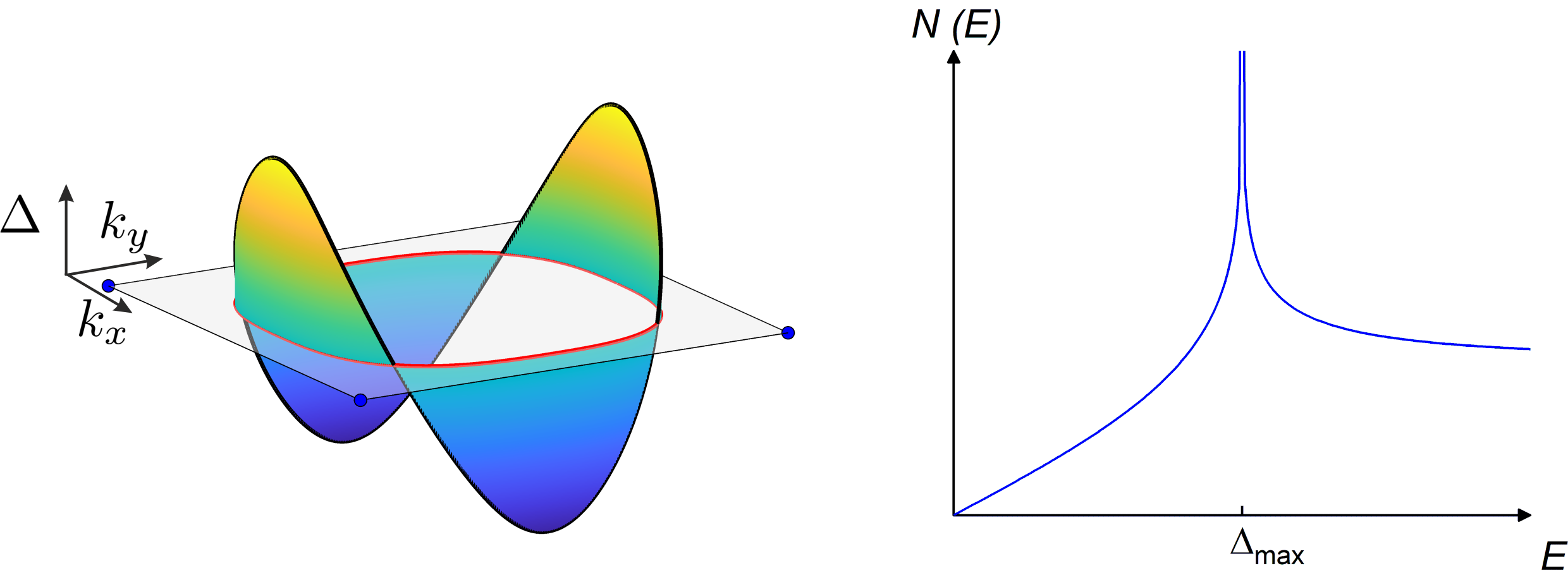
Nodes have important experimental consequences since they determine the low temperature behavior of quantities such as specific heat moler and penetration depth hardy . This arises through the thermal population of quasiparticles, whose occupation number,
| (5) |
involves the excitation energy,
| (6) |
is the band energy measured relative to the chemical potential. The right panel of figure 1 shows the density of quasiparticle states for the gap. For a gap without nodes there are no states below . Nodes lead to a linear contribution . As shown in figure 2 , below about the gap function is nearly temperature-independent. The low temperature variation of the penetration depth then comes entirely from the variation of the gap in -space. The linear quasiparticle density of states leads to a power law temperature dependence while a finite gap everywhere on the Fermi surface leads to an exponentially-activated dependence. Low temperature measurements with sufficient precision can therefore indicate the presence of nodes, or at least place a lower limit on magnitude of the gap. It would seem that experiments relying solely on quasiparticle occupation cannot distinguish a state with nodes but no sign change from the sign-changing state. However, we will see that the sign change of the -wave gap function, though more directly accessible through Josephson and flux quantization measurements dale ; tsuei , can reveal itself through penetration depth measurements at low temperatures. Later, in our discussion of multiband superconductors, we discuss how measurements together with controlled impurity scattering can also lead to phase sensitivity.
Many of our measurements focus on the region well below where the temperature dependence of the gap function can be ignored, regardless of its momentum dependence. Within the weak-coupling (BCS) approximation the pair interaction is assumed to have the form, . This leads to a gap function of the general form,
| (7) |
where the average taken over the Fermi surface. is obtained by solving the following self-consistent equation KP2021PRB ,
| (8) |
The brackets denote a Fermi surface average and are Matsubara frequencies. A very good approximation for the temperature dependence of the gap function is given by KP2021PRB ,
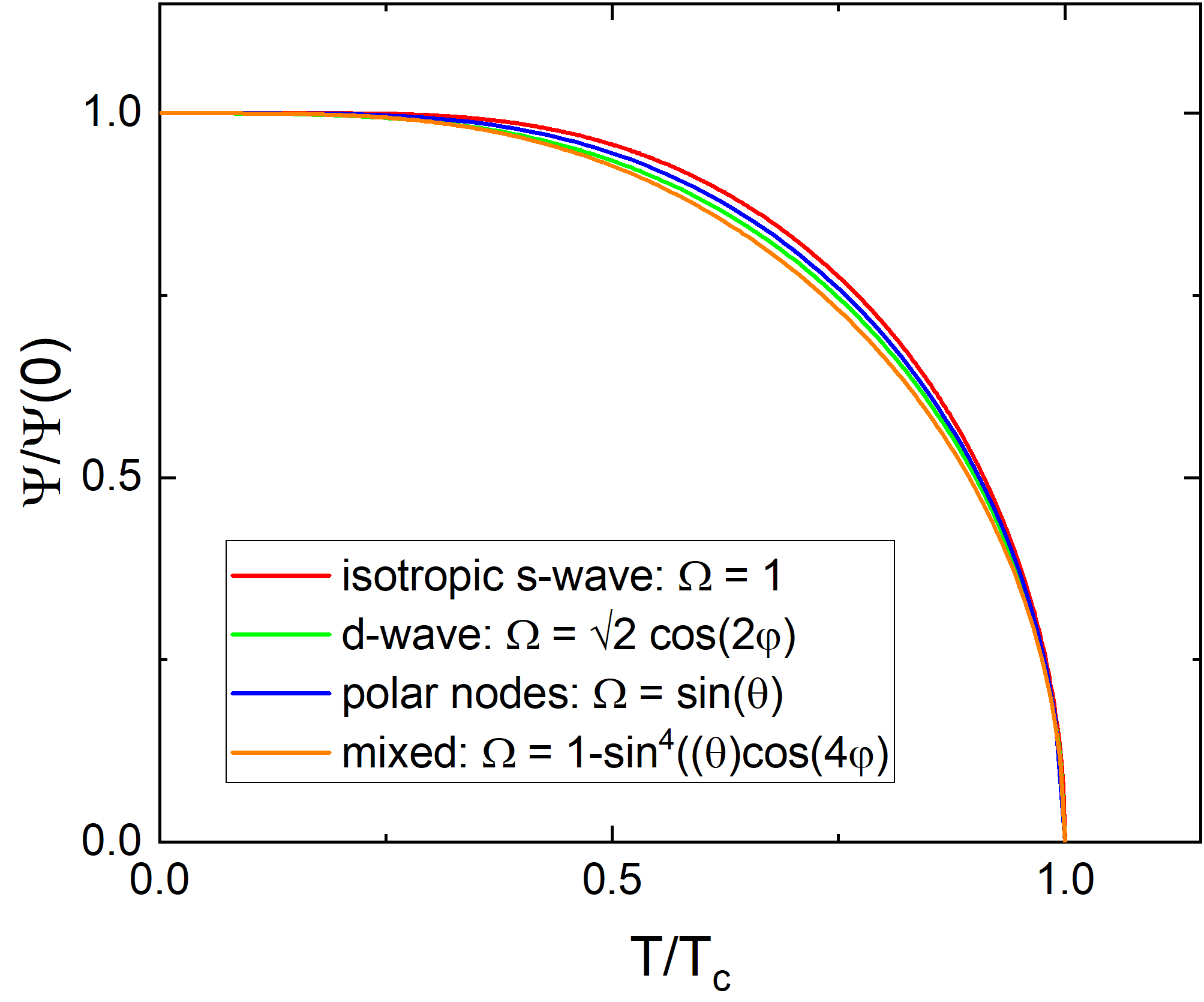
| (9) |
where = is Euler’s constant and = is the Riemann zeta function. Figure 2 shows that the ratio in equation 9 is a nearly universal function of and only weakly dependent on the -variation of the gap function. Furthermore figure 2 shows that is nearly temperature independent below , regardless of the dependence of the gap. The approximately universal temperature dependence does not hold for multiband superconductivity where different gap functions exist on different Fermi surface sheets.
3 Penetration depth and superfluid density
The basic experimental feature of a superconductor is perfect diamagnetism, i.e., the Meissner effect. Using the second London equation and Ampere’s law the magnetic field in a superconductor obeys,
| (10) |
where is the London penetration depth. Equation 10 implies that an applied magnetic field decays exponentially into a superconductor on the length scale of . More generally, the penetration depth is anisotropic. The second London equation then relates the supercurrent components to the vector potential through a superfluid density tensor ,
| (11) |
where we assume the London gauge, . The measured penetration depth components are then obtained from the principal axis components of . therefore refers to the penetration depth for the current , not the field component . In layered superconductors such as copper oxides, , the penetration depth for currents within the conducting planes is quite different from , the penetration depth for interplane currents. Unless otherwise noted we will denote the in-plane penetration depth as simply .
Microscopic treatments of the penetration depth can be found in many excellent texts and articles. For the present we recall a useful semiclassical result which holds in London limit where the current is locally proportional to the vector potential gross ,
| (12) |
The factors are Fermi velocities along the direction, while the gap function and quasiparticle energy were introduced earlier. Equation 12 consists of two competing terms. The temperature-independent term comes from a diamagnetic current that is present in both normal and superconducting states when a magnetic field is applied. It is proportional to the full density of carriers and does not depend on the superconducting parameters. The second term comes from a paramagnetic current that depends on both the gap function and the temperature tinkham . This term defines the normal fluid density . The superfluid density is given by the difference = - . Above , the two currents cancel, vanishes and the penetration depth is infinite. In liquid helium physics one directly measures the superfluid density but in superconductivity it is that is more often measured.
Figure 2 shows that below approximately 0.25 the energy gap for and wave pairing is essentially temperature independent. In this region we can use equation 12 to find the temperature dependence of the normalized superfluid density (also known as the phase stiffness). For -wave pairing we recover the standard BCS result,
| (13) |
For a -wave gap function, where . Assuming an isotropic or spheroidal Fermi surface, is linear at low temperatures prozorov1 ,
| (14) |
More generally, for a superconductor with line nodes,
| (15) |
where the denominator is the slope of the gap angular dependence at the node Xu95 . The predicted linear temperature dependence arising from nodal quasiparticles was first measured in optimally doped YBa2Cu3O6+x (Y123) crystals by Hardy et. al. hardy using a superconducting microwave resonator. This important experiment was crucial to the wide acceptance of nodes in the gap function of copper oxide superconductors and gave support to the hypothesis of -wave pairing in these materials. The temperature dependence is crucial since the in-plane magnetic response (equation 12) is isotropic for a -wave superconductor with tetragonal lattice symmetry. Therefore, changing the direction of the magnetic field cannot distinguish -wave from -wave.
For an arbitrary angular variation of the gap, , the amplitude is found by solving equation 8 at zero temperature, after which the nodal derivative is determined. The shape of the Fermi surface affects through its dependence on at the node, as indicated in equation 12. The nodes may also be inequivalent, in which case separate derivatives must be calculated.
The issue of strong versus weak coupling sometimes arises in the interpretation of data. Strong coupling increases the magnitude of the gap relative to so it is more likely to extend the low temperature region over which power laws are determined by the dependence of the gap function. For a -wave superconductor, the coefficient of in equation 14 is affected by the magnitude of gap function but it is also affected by its specific shape in space and the details of the Fermi surface, so strong coupling effects are difficult to isolate. Kogan and Prozorov KP2021PRB have shown that claims of strong-coupling obtained by fitting to an exponential dependence of can often be erroneous. Later, we discuss two band superconductors. There, weak coupling implies a generalization of the familiar , = criterion tinkham to a matrix that involves the pair interaction both within and between bands.
4 Nonlinear Meissner Effect
The development of our technique for measuring penetration depth was motivated by a theoretical paper by S. Yip and J. Sauls ys which suggested that penetration depth measurements as a function of magnetic field could provide a stringent test of -wave pairing and potentially locate the directions of the nodes of the gap function. They termed this phenomenon the nonlinear Meissner effect and predicted that it would be observable at low temperatures in sufficiently pure Y123 crystals. For a simple picture, recall that the energy of a quasiparticle in the BCS state depends on the direction of its momentum relative to the net superfluid velocity ,
| (16) |
Quasiparticles with momentum parallel to have higher energy than those antiparallel, i.e., a Doppler shift. The counter-moving excitations reduce the net supercurrent and therefore increase the penetration depth. The penetration depth is also increased by the field in a fully-gapped superconductor but the effect is small, the correction being of order where is a scaling field of order the thermodynamic critical field. In addition, the correction vanishes exponentially with temperature due to the presence of a finite energy gap everywhere on the Fermi surface.
Yip and Sauls showed that -wave pairing changes the picture entirely. Due to the presence of nodes, counter-moving quasiparticles in the -wave state are more likely to be populated by the application of a field. This occurs at fields low enough that suppression of the gap itself by the field is small. The repopulation reduces the supercurrent and leads to an increase of the penetration depth that is linear in the applied field. At finite temperature this correction is reduced at low field () so the total change with field grows as the temperature is reduced. Their prediction at = was,
| (17) |
where is predicted to be larger for node compared to node. The observation of a nonlinear Meissner effect posed a significant experimental challenge. The need to work in the Meissner state requires (about 100 Oe for plane of Y123 ) while T in Y123. The largest predicted field-dependent correction to is less than 1 percent. Since 1500 Å, it was necessary to resolve Angstrom-level changes in using crystals whose maximum dimension was typically less than 1 mm.
The need to apply a DC magnetic field in addition to a tiny RF probing field ruled out a superconducting microwave resonator approach. One of us (RWG) recalled a Cornell low temperature physics group seminar given in the late 1970’s by Craig Van Degrift. He had built an extremely stable tunnel diode resonator (TDR) to measure tiny changes in the dielectric constant of liquid helium vDG . The device operated at a few MHz using a copper coil and a capacitor for the resonant cavity. The high sensitivity and absence of superconducting components suggested that the TDR would be an ideal device to search for the nonlinear Meissner effect.
5 Measurement of Penetration Depth
Using the London equation it is a standard exercise to show that the induced magnetic moment of a superconducting slab in a uniform magnetic field is given by,
| (18) |
Here , where , and are the length, width and thickness of the slab. The field is applied parallel to the longest dimension therefore minimizing demagnetizing effects. In our measurements is an RF field. Unfortunately, a thin slab, a sphere and a cylinder are the only shapes for which the London equation can be solved exactly. The irregular shapes encountered in experiments can usually be treated with the following approximate expression,
| (19) |
where is a demagnetizing factor and is an effective sample dimension for which Prozorov et al. derived an approximate analytical expression prozorov1 ; prozorov2 . If the sample is now inserted into the coil of an oscillator, the oscillation frequency increases by an amount,
| (20) |
where depends on the effective volume of the coil and the oscillation frequency. While the prefactor is difficult to calculate reliably, it can be directly measured by removing the sample from the coil in situ at the base temperature where the -dependent term is typically or smaller. For typical sample sizes, the frequency shift in equation 20 ranges from 1 100 kHz and repeats to within 1-2 ppm. Once has been obtained, we measure the change in resonator frequency as the temperature or an external DC magnetic field is varied. A more complete account of the calibration, including updated formulas for the effective dimensions can be found in ref Prozorov2021 .
The small size of the -dependent term in means that one cannot simply insert the sample into the coil, measure the change in oscillation frequency and determine . To do that would require knowing the sample geometry, field orientation and then numerically solving the London equation for , all with far more precision than is currently feasible. What can be done is to numerically calculate the effective sample dimension in equation 19, measure the change in frequency as the sample temperature changes and convert that change into = to a precision of a few percent. The normalized superfluid density is then given by,
| (21) |
The zero temperature penetration depth is often obtained from other techniques such as SR, small angle neutron scattering or infrared reflectively. These techniques have far less sensitivity to but can determine to reasonable precision. Later, we will discuss an aluminum-plating technique which allows us to measure the full value of with the tunnel diode resonator alone.
Commercial magnetometers lack the sensitivity for the measurements discussed here. For example, a perfectly diamagnetic cylinder 1 mm in diameter and 0.1 mm thick (slightly larger than our typical sample) has a moment emu (1 emu = erg/G). A change in penetration depth for this sample corresponds to a change in magnetic moment . For 1 Å this corresponds to emu, approximately 4 orders of magnitude smaller than the sensitivity of commercial magnetometers. However, the required sensitivity can be attained with a tunnel diode resonator.
6 Tunnel Diode Resonator
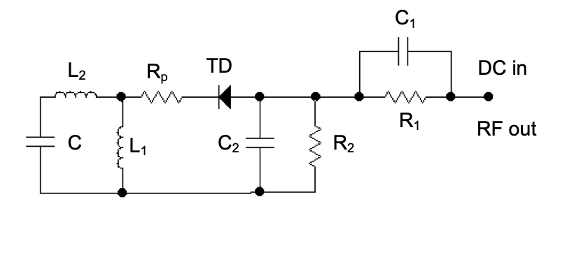
Tunnel diode resonators have been used in low temperature physics since the 1960’s heybey ; boghosian ; tedrow . Their advantages include simplicity, high sensitivity, low power dissipation and the ability to operate in static magnetic fields of many Tesla. Figure 3 shows the IV characteristic of a BD3 tunnel diode. At the inflection point the diode has its peak negative differential resistance , , which will lead to sustained oscillations when incorporated into the circuit shown in Figure 4. is the sample coil and is a tap coil that adjusts the impedance of the tank circuit, making the oscillator ‘marginal’ which reduces substantially the frequency noise levelvDG . is used to reduce parasitic resonances. The other resistors maintain the correct DC bias while and couple the RF signal out of the oscillator and provide an AC ground, respectively. At resonance, the tapped tank circuit presents a resistive impedance where is the quality factor, is the coil AC resistance and is the tap fraction. The resonant frequency is typically 10-15 MHz. Typically, oscillations do not begin until well below 77 K when the onset condition is met. There are many small corrections to the frequency that depend on and the other circuit component values but these are independent of the superconducting sample properties and are therefore constant throughout the measurement. Dissipation in the sample can affect and therefore the oscillation frequency but this effect is negligible except very close to .

The sub-mm dimensions of many superconducting crystals dictate the size of the sample coil . It must be small enough to be measurably perturbed by Angstrom-level changes in penetration depth yet large enough to generate a homogeneous RF magnetic field. Ours are typically 1 cm long and 2 mm in diameter with a quality factor = 100-200. The coil is surrounded by a copper tube which makes the field more homogeneous, lowers its amplitude and provides temperature stability. The tunnel diode circuitry sits inside a shielded enclosure whose temperature is controlled near 2 K to within a few K.
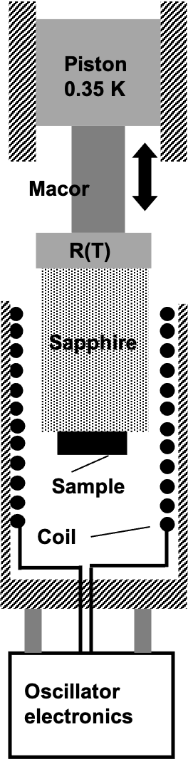
Figure 5 shows a schematic of a typical apparatus carrington ; organic . The sample is attached to a sapphire rod that can be moved in and out of the tunnel diode oscillator coil. The thermometer and heater stage, R(T), is located at the opposite end of the rod, outside the RF field of the coil. The thermometry stage is in turn attached to a low thermal conductivity ceramic rod which is attached to a copper piston that slides inside a closely fitting copper cylinder. The cylinder and piston are heat sunk to the 3He evaporator. This scheme allows the sample temperature to be controlled anywhere from 0.35 – 150 K, independent of tunnel diode circuit. The latter is independently controlled near 2 K but mechanically attached to the cylinder/piston assembly through a graphite tube. DC magnetic fields both parallel and perpendicular to the axis of the sapphire rod are applied with small superconducting coils inside the vacuum can. The ability to control the oscillator temperature independently of the sample temperature and to remove the sample from the RF field in situ have proven to be indispensable for both calibration purposes and for eliminating frequency shifts due to applied magnetic fields. Variations on this design have been used with a dilution refrigerator to achieve sample temperatures below 50 mK bonalde ; bonalde2 ; fletcher2007 ; fletcher2009 ; tanatar ; wilcox .
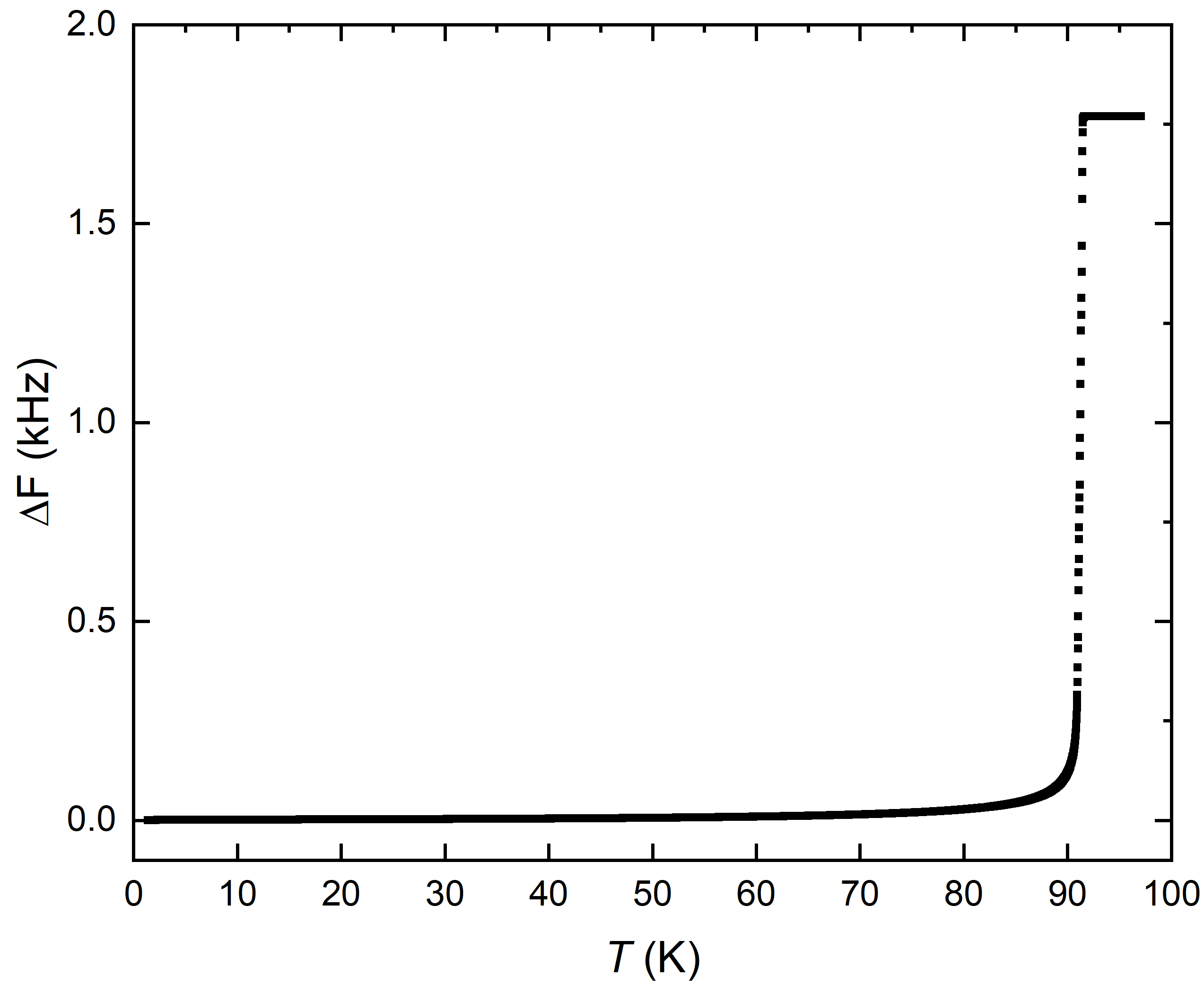
Figure 6 is an example of resonator data for a optimally doped single crystal of YBa2Cu3O6+x with and size . Above the curve is nearly flat due to the skin depth being larger than the sample thickness. The sharp transition at is a useful check on the thermometry and sample homogeneity but it tells us little about the superconducting state beyond the existence of a Meissner effect. With the vertical scale shown, the data for all superconductors looks very similar. To distinguish an exponential from a power law temperature dependence we must work at temperatures well below and with the vertical scale expanded by 100-1000 depending on the sample size.
7 Search for Nonlinear Meissner Effect
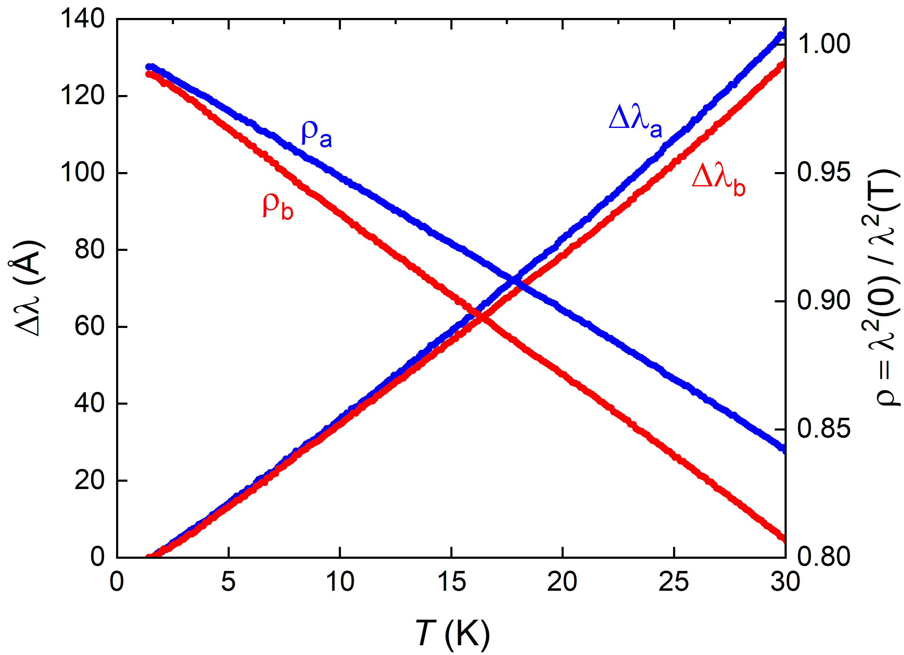
In the first application of the apparatus, Carrington et. al. carrington measured the temperature dependence of the penetration depth in a Y123 crystal. Figure 7 shows and for supercurrents along the and directions in the copper-oxide plane. We reiterate that are the directly measured quantities while the use reported values of as inputs. While all four quantities vary linearly at the lowest temperatures, the superfluid density is linear over a wider range than , as expected. Our values of were within a few percent of those obtained by Hardy et al. hardy .
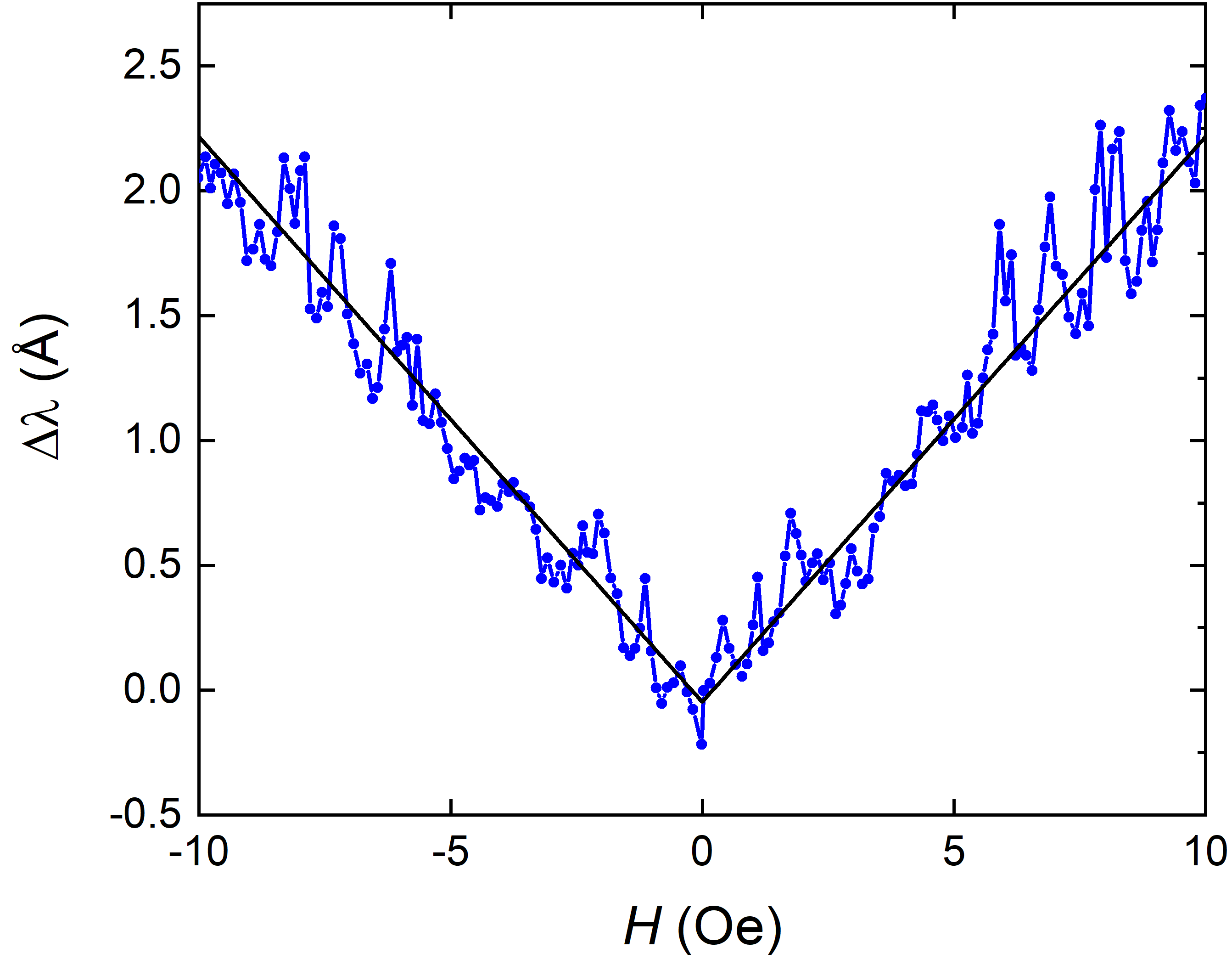
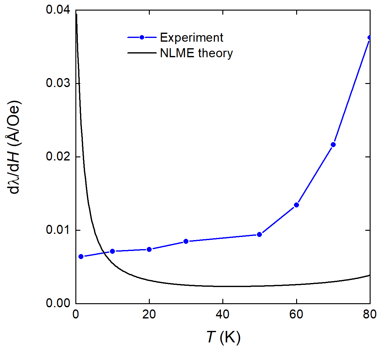
Our goal was to measure the magnetic field dependence of and this data is shown in figure 8. While we routinely observed a linear dependence, the data lacked other characteristics we were looking for. Y123 is a type II superconductor so it admits quantized vortices. Despite applying fields below the accepted lower critical field, it appears that vortices can still enter the sample and generate a field dependence to , possibly at the corners of the sample where the demagnetising effects are higher. In the mixed state, field dependent changes in occur because the RF-field imparts a Lorentz force to a vortex. The oscillating vortex carries magnetic field into the superconductor and therefore increases the total penetration depth. This vortex contribution, known as the Campbell penetration depth, adds in quadrature with the desired contribution from the Meissner state:campbell1 ; campbell2 ; prozorov3 ; wu ; tea ,
| (22) |
Treating the vortex as a particle in a harmonic pinning well subject to an oscillating Lorentz force, the Campbell depth is given by,
| (23) |
where is the flux quantum and is the effective force constant of the pinning well. A recent, more comprehensive treatment of the Campbell depth may be found in ref. willa . For small fields, the Campbell depth also leads to a linear magnetic field dependence to the measured penetration depth. However, with increasing temperature, vortex pinning weakens, decreases and the Campbell contribution to the penetration depth , precisely the opposite of the nonlinear Meissner effect. As shown in figure 9, an increase of with temperature is what we observed particularly closer to , thus pointing to vortex motion as the cause. We reluctantly published a null result for the nonlinear Meissner effect in Y123 carrington as did Bidnosti et. al. bidnosti who used a low frequency mutual inductance bridge method to look for the effect. Previously, Sridhar et. al. sridhar had used a TDR to study in Y123 and concluded that the field dependence was consistent with pair-breaking in an -wave pairing state. Later, Maeda et. al. et. al. maeda used a TDR to observe a linear field dependence to in Bi2Sr2CaCu2Oy. Although they claimed to have observed the nonlinear Meissner effect, in their samples had a quadratic (rather than linear) temperature dependence, indicating inadequate purity. In addition, they found to be only weakly dependent on temperature, in contradiction with the theory shown in figure 9, and again suggesting that vortex motion was responsible for their observed field dependence.
It is worth pointing out that the apparent noise in figure 8 is actually highly reproducible. Subtracting away the linear trend leaves an oscillation with a period of about 0.5 Oe, almost certainly coming from a modulation by the DC field of the critical current in weak links somewhere in the sample. In other superconductors we have observed such oscillations with periods of only a few mOe. This places an upper limit on the RF field amplitude since the oscillations would not be observable unless the RF field were much less than the DC field periodicity of a few mOe.
Recently Wilcox et al. wilcox have succeeded in observing the nonlinear Meissner effect in non-copper oxide superconductors, CeCoIn5 and LaFePO. These are also nodal superconductors but have a much lower (2.3 K and 6 K respectively) than optimally doped Y123. As does not depend on but does, it is expected that the field-dependent change in at the maximum field before vortices enter varies as . Therefore the non-linear Meissner effect is much easier to see in these low- materials. The effect is likely also present in Y123 but is masked by extrinsic effects such as vortices (above) and Andreev bound states as described below.
8 Surface Andreev Bound States
The -wave order parameter changes sign in -space and it was soon appreciated that this would to lead to current-carrying states localized near particular crystalline faces hu ; tanaka ; fogelstrom ; barash . These so-called surface Andreev bound states (ABS) can arise in the geometry shown in figure 10 where the -wave gap function is superimposed on a crystal with a [110] facet. The oppositely-signed lobes of the gap function present an effective potential for quasiparticles moving along the trajectories shown, leading to zero energy bound states that live within a few coherence lengths of the [110] surface. These states carry current and their presence leads to a peak in the quasiparticle density of states at zero energy and consequently a dependence for that appears below about 10 K in Y123 crystals. Moreover, the contribution from bound states is predicted to vanish in small magnetic fields as the bound state energy is pushed away from the Fermi energy by the Doppler shift in quasiparticle energies caused by the screening currents.
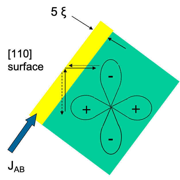
Magnetic impurities may also lead to a paramagnetic upturn in pcco . Given the unusual nature of surface Andreev bound states, it was important to distinguish the two. Observations by Carrington et al. carringtonabs satisfied several criteria for the upturn. (1) It appears below approximately 10 K in Y123 (2) Its magnitude is a function of the angle between the actual crystal face and the [110] direction (3) It appears only with induced supercurrents confined to the sample edges (4) It is quenched with a small ( 100 Oe) DC magnetic field. Magnetic impurities would satisfy none of these criteria.
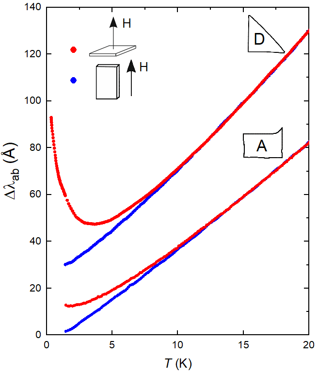
Figure 11 shows data for two crystals with differing amounts of [110] surface and with the RF field in two orientations. With the field normal to the planes, induced supercurrents circulate around the perimeter of the crystal and penetrate in from the edge on a length scale of , the in-plane penetration depth. This orientation is expected to show the upturn since it is most sensitive to the bound state current on [110] faces. If the RF field is oriented parallel to the planes, supercurrents flow across the top and bottom faces where there are no bound states so no upturn is expected. Figure 11 shows the result for each RF field orientation in two different crystals. In each crystal, an upturn was observed only for the predicted RF field orientation and the size of the upturn scaled as predicted with the amount of [110] surface present. Paramagnetic upturns in below were also reported in thin films of Y123 by Walter et. al. walter Those authors used heavy ion irradiation to generate tracks with varying amounts of [110] surface. The size of the upturn scaled with the estimated amount of [110] surface] as expected for surface Andreev bound states. They did not report measurements of the magnetic field dependence of .
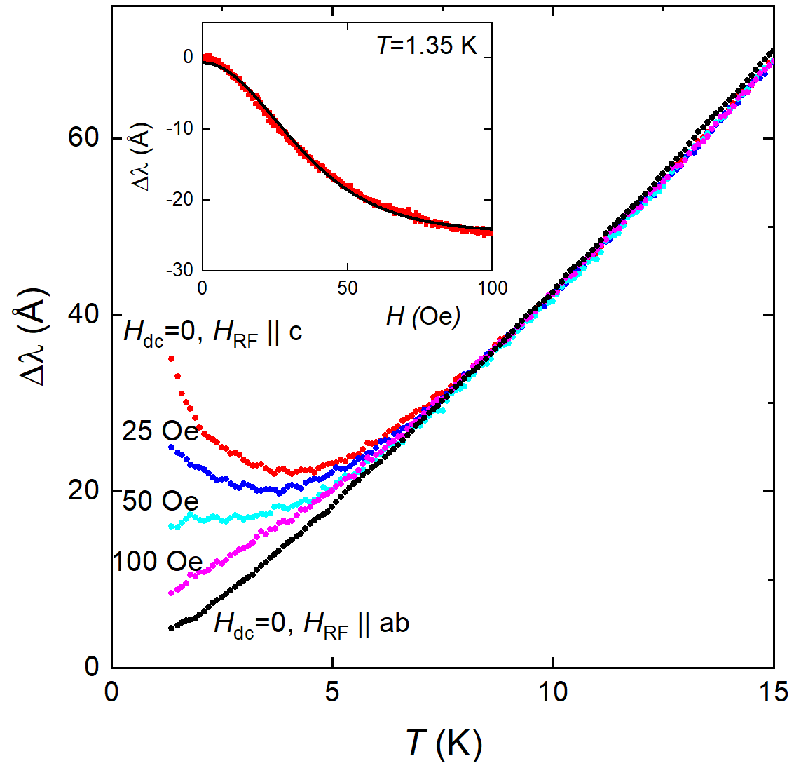
Figure 12 shows how the upturn in is quenched in a dc field of 100 Oe, which is remarkably small. Were the upturn coming from magnetic impurities, the penetration depth would be enhanced by a factor of where is the magnetic susceptibility. Assuming an impurity magnetic moment , and spin , a field of 3 Tesla would be required to reduce by 95 percent. The much smaller field scale arising from Andreev bound states can be understood from a simple model in which bound states contribute a delta function peak to the density of states at an energy given by the Doppler shift in equation 16 (). This leads to a field-dependent upturn given by,
| (24) |
Here is the Fermi velocity and is a function of the angle between the surface normal and the [110] direction beta . The inset shows a fit to Eq. 24. A more accurate theory barash includes the necessary averaging over the Fermi surface and the effect of finite quasiparticle lifetime (scattering). Fitting to that theory gives results which are similar to Eq. 24, but with a higher value of . In fact, is essentially the only free parameter and was determined to be ms-1, similar to other estimates. Bound states do not occur unless the gap function changes sign so these observations were strong evidence for the unconventional, pairing state first proposed for the copper oxide superconductors. Tsai and Hirschfeld tsai later pointed out that both the 1/T upturn and its suppression by low magnetic fields could arise from sufficiently isolated, unitary-limit impurity scatterers in a d-wave superconductor. Their mechanism does not predict the dependence on crystal shape ([110] surface) that we observed, but it may account for earlier observations of a low temperature upturn in for Zn-doped Y123 bonn2 .
9 Multiband superconductors
Penetration depth measurements in the high temperature superconductors focused on the gap function in materials with simple Fermi surfaces. In the majority of superconductors, pairing occurs on multiple Fermi surface sheets but the scattering of electrons between sheets effectively homogenizes the gap function. However, in materials where the Fermi sheets have distinct orbital character, interband scattering is strongly suppressed resulting in distinct gap functions for each sheet, i.e., multiband superconductivity. We present two examples. The first is MgB2, a phonon-mediated superconductor with K. The second is CaKFe4As4 ( K) a member of the large class known as iron-based superconductors hosono in which the pairing appears to be mediated by magnetic interactions mazin ; hirschfeld2011 .
While measurements of for are necessary for detecting nodes and sign changes in the order parameter, measurements over the entire temperature range up to are required to identify multiple gaps. Over this full range, as figure 6 shows, the penetration depth looks essentially flat while the superfluid density is far more revealing. Figure 13 shows the results for MgB2fletcher . Superfluid densities and correspond to screening currents along the and axes of the crystal. Pairing in MgB2 occurs on different Fermi surface sheets (), each with its own superfluid density (, ) and gap function (, ). The temperature dependence of each gap is show in the inset. The fits in figure 13 were produced using a weighted sum,
| (25) |
with = 75 K and = 29 K and for each band calculated using a 2-band Eliashberg model. The temperature dependence of is close the the isotropic BCS model but for there are significant differences. A fully self-consistent analysis of the experimental data in MgB2 can be found Ref.Kim2019 and is outlined below.
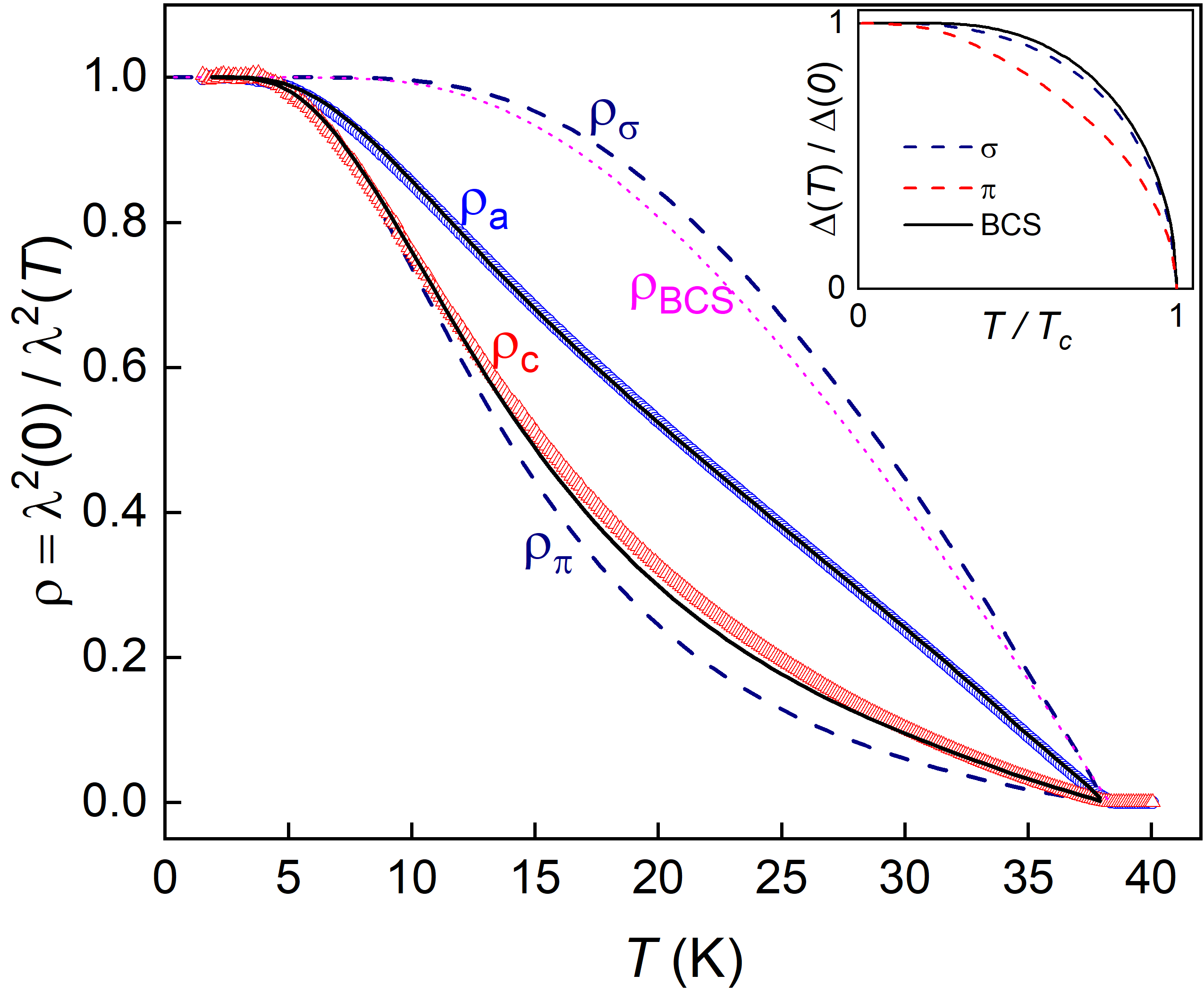
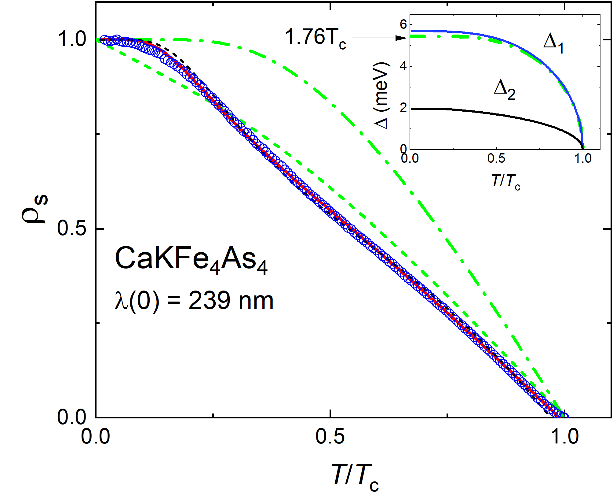
Figure 14 shows the superfluid density for CaKFe4As4, a stoichiometric iron-based superconductor Cho2017 . To generate from the value of was taken from the new technique of optical magnetometry using nitrogen vacancy (NV) centers in diamond Hc1PRA2019 . The solid line is a fit to a self-consistent model of two-band superconductivity involving both in-band and interband pairing interactions as well as two intraband and one interband scattering rate Kogan2009 ; prozorov2011 . For comparison, we also show the superfluid density for a single band -wave (green solid line) and -wave (green dashed line) gap functions. Both differ significantly from the two-band model, which provides an excellent fit. The inset shows the gap for each band (, ) calculated self-consistently using a two-band generalization of Eq.8 Kogan2009 . Although the temperature dependence of and are reasonably close to the standard BCS form, one gap is always larger and the other is always smaller than the weak-coupling BCS value.
An idealized material with only in-band pair interactions would exhibit separate superconducting transitions. In real materials an interaction always exists and there is just one transition but the shape of retains some remnant of the idealized case, sometimes leading to the positive curvature shown by in figure 13. However, this alone cannot be considered proof of multiband superconductivity and other measurements are needed. These two examples show that precise penetration depth measurements over the full temperature range, coupled with sophisticated analysis, can now reveal the details of multiband superconductivity.
10 Impurity scattering
Real samples contain impurities, which can substantially alter the temperature dependence of . While phenomena such as nonlinear Meissner effect and Andreev bound states require the highest purity samples, the deliberate addition of impurities has historically been an important probe of superconductivity. Anderson’s theorem anderson states that non-magnetic impurities do not change in an isotropic superconductor. When they do lower a more complicated pairing state is likely to be involved. Impurities may also alter the power law for the temperature dependence of the penetration depth. The tunnel diode method permits us to measure with remarkable precision and therefore discriminate among different possible gap functions. Quantitative predictions for the effect of impurities require more advanced mathematical techniques so we will state only the final results Xu95 ; prozorov2011 ; bang ; vorontsov .
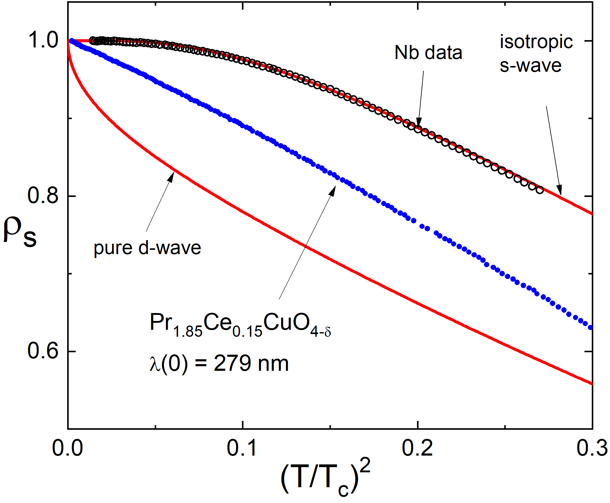
Early measurements in the copper oxides showed a quadratic power law . This was later shown by Hirschfeld and Goldenfeld to result from non-magnetic impurity scattering in the unitary (strong scattering) limit that generates quasiparticle states at = 0 without a concomitant sizeable reduction in in a -wave superconductor hirschfeld1993 . Their empirical formula, valid in the domain ,
| (26) |
includes a crossover temperature related to the density and strength of scatterers. For , and for , . Figure 15 shows the superfluid density for the electron-doped copper oxide Pr1.85Ce0.15CuO4-δ ( K) pcco . For this material in the low temperature region shown. The = 2 power law is clearly distinct from the exponential variation seen in Nb and was taken as early evidence for -wave pairing in the electron-doped copper oxides pcco .
Penetration depth measurements with added impurities have been particularly useful in revealing the pairing state of the iron-based superconductors. Since these are multiband superconductors, different gap magnitudes, nodes and sign changes are all possible. Figure 16 illustrates four possible pairing states in the iron-based materials hirschfeld2011 . In each case, the central surface is hole-like while the four adjacent ones are electron-like. The leading candidate for most iron-based superconductors is the state in which hole and electron surfaces are each fully gapped, albeit with different gap amplitudes and a sign change between them. This state is favored by a repulsive interaction coming from the exchange of spin fluctuations between electron and hole sheets mazin ; hirschfeld2011 . Since it has 4-fold rotational symmetry, the state is still conventional in a group-theory sense but the sign change leads to measurable consequences. Interestingly, while Anderson’s theorem remains applicable for in-band scattering, nonmagnetic interband scattering is pair-breaking if the gap function changes sign between bands Kogan2016 ; prozorov2011 .

Measurements on clean samples cannot easily distinguish from . In each case, shows an exponential dependence at low temperatures characterized by the smaller of two gaps. However and superconductors respond differently to the addition of non-magnetic scatterers. At low temperatures, in an superconductor continues to show exponential dependence but in an superconductor it is predicted to evolve from exponential to with increased scattering bang ; vorontsov . At our current level of sensitivity, is nearly indistinguishable from exponential behavior so the prediction for is effectively a decrease of toward = 2 with increased scattering. This contrasts with the case for a -wave superconductor with line nodes, in which more scattering leads to an increase of from 1 to 2. The peculiar situation for comes from the generation of new quasiparticle states below the minimum energy gap with increased scattering. The top panel of Figure 17 shows the calculated density of states in an superconductor for two levels of impurity scattering Kim2010 . For weak scattering, two sharp gap features are apparent along with a small midband density of states. Increased scattering broadens the distribution and generates new states at = 0 leading to .
Experiments of this type are sometimes complicated by changes in carrier density when impurities are added. Columnar defects produced by heavy ion irradiation offer one way around this problem. This approach was used to vary the density of defects in the electron-doped pnictides Ba(Fe1-xCox)As2 and Ba(Fe1-xNix)As2, as shown in the lower panel of Figure 17. Here is plotted versus the exponent with the defect density as an implicit variable. Both and vary exactly as predicted from the density of states calculated for an order parameterKim2010 .

While the numerical details depend on specifics of the Fermi surface and scattering rates, the evolution of the power law from high to low and the concomitant change in is a qualitative result that provides some of the strongest evidence for pairing. Impurity experiments like this may also be useful in identifying topological superconductivity in materials such as the Dirac semimetal, PdTe2 PdTe2eirr2020 .
11 Absolute penetration depth and quantum criticality
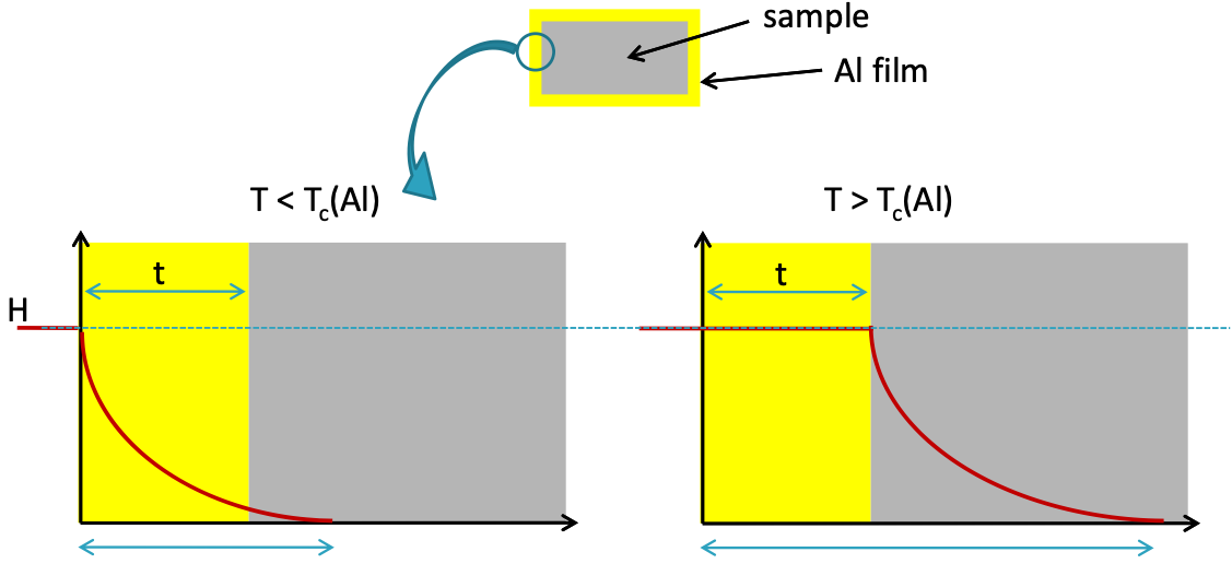
Although the tunnel diode resonator can easily measure changes in with very high precision, absolute measurements are considerably more difficult. Nonetheless, the sensitivity to changes in resonator frequency can be exploited using the scheme shown in Figure 18 Alcoating . Here, the sample under study is uniformly sputter-coated with aluminum to a depth of typically 1000 Å. Since the skin depth of Al at 10 MHz is much larger than 1000Å, the film is invisible to the RF field when and the effective penetration depth is . This case is shown on the right panel. As the sample cools below the film becomes superconducting and the RF field penetrates the composite superconductor shown in the left panel. Treating each superconductor in the London limit, the effective penetration depth of the composite is given by,
| (27) |
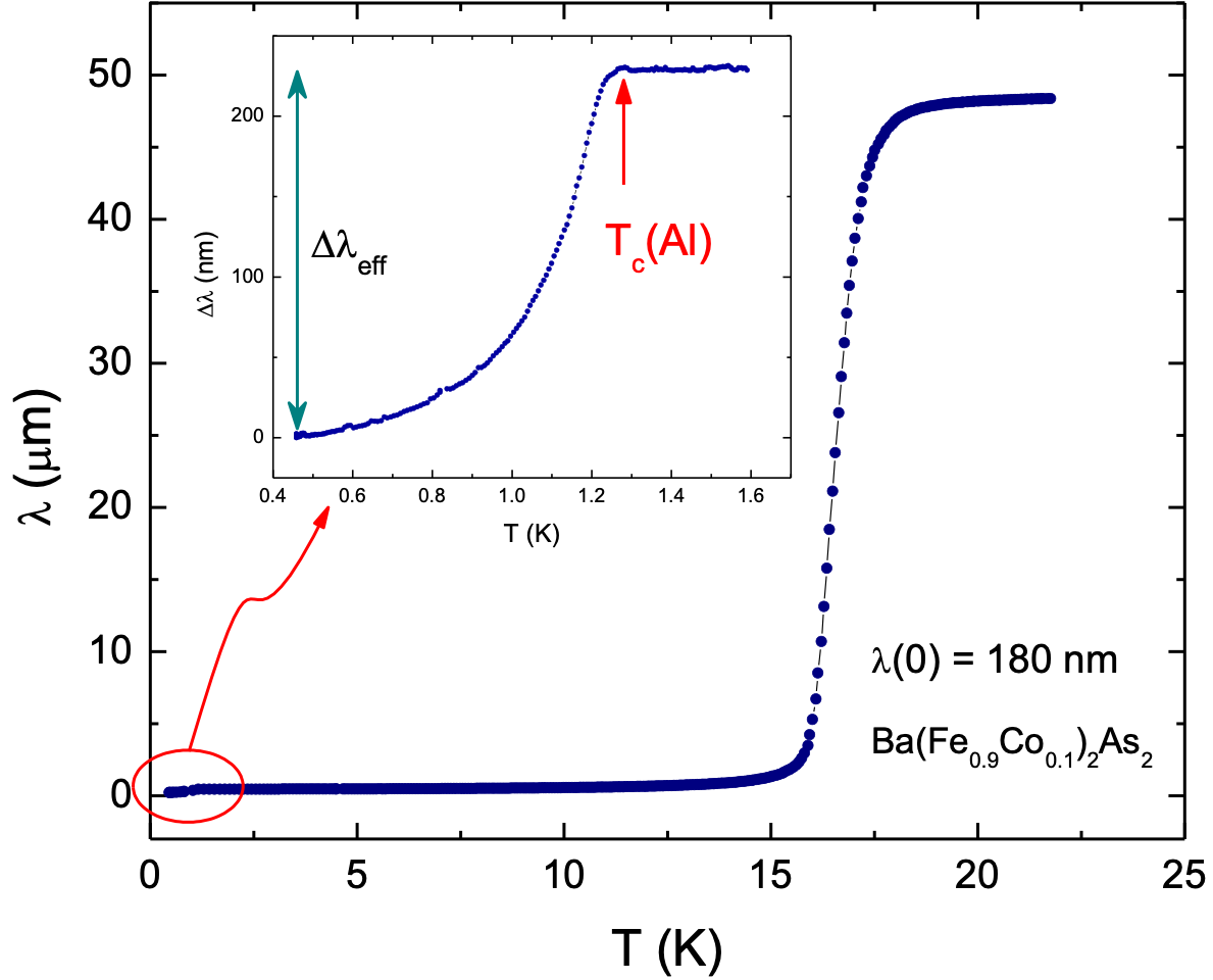
By measuring the (shown in the insert) and assuming Åtedrow we can extract of the underlying superconductor. Since K is well below that of the underlying superconductor, we essentially measure its zero-temperature penetration depth, . An example is shown in Figure 19 for Ba(Fe0.9Co0.1)2As2. The inset shows the transition to superconductivity in the Al film. The inset shows the transition to superconductivity in the Al film. Although there is some uncertainty in because of disorder and surface roughness of the film meservey , the technique generates values of for several copper oxide and iron-based superconductors that are in good agreement with other experimental methods.
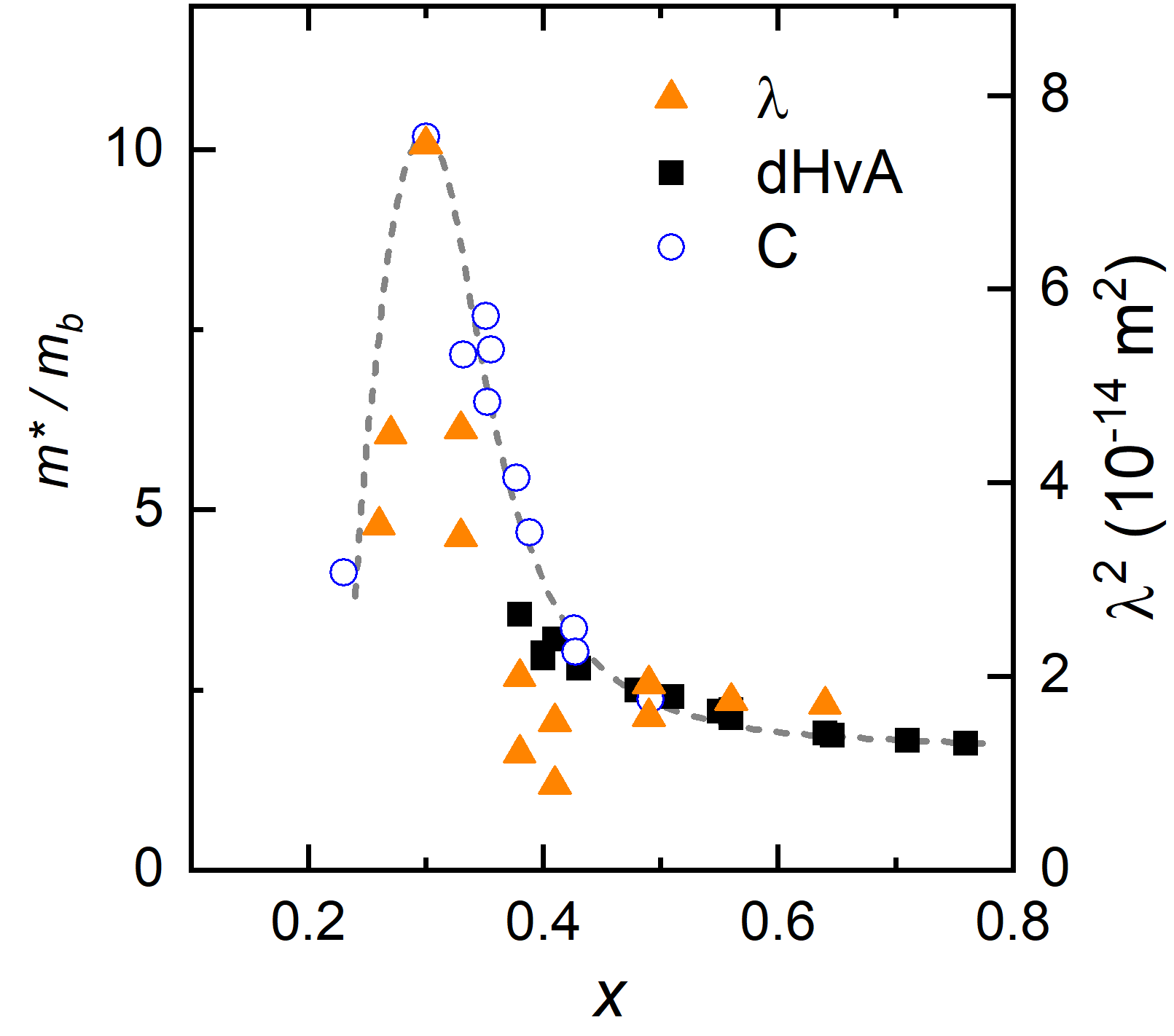
In a simple picture (Eq. 12) is proportional to the ratio of the normal state parameters , where is the volume of the Fermi surface. In the BaFe2(As1-xPx)2 (BaAsP122) system quantum oscillation measurements have shown that varies markedly with , peaking at the composition , which corresponds to a quantum critical point (QCP) of the antiferromagnetic phase Hashimoto2012 ; walmsley . Measurements of using the Al plating method also showed a peak at in which the mass enhancement derived from was found to be in good agreement with those derived both from quantum oscillations and specific heat. This data is shown in figure 20 Hashimoto2012 ; walmsley ). This peak in mass is important evidence that is boosted by the presence of the QCP. There is some theoretical uncertainty about how mass renormalization enters the expression for . For a Galilean invariant Fermi-liquid the mass renormalization is cancelled out by backflow at (leggett ), so in Eq, 12 is the bare band mass. However, it is unclear to what extent this applies to a solid which is not Galilean invariant and the presence of electron and hole pockets may also break the backflow cancellation Levchenko ; nomoto . The BaAsP122 system is the clearest system to date where this has been tested.
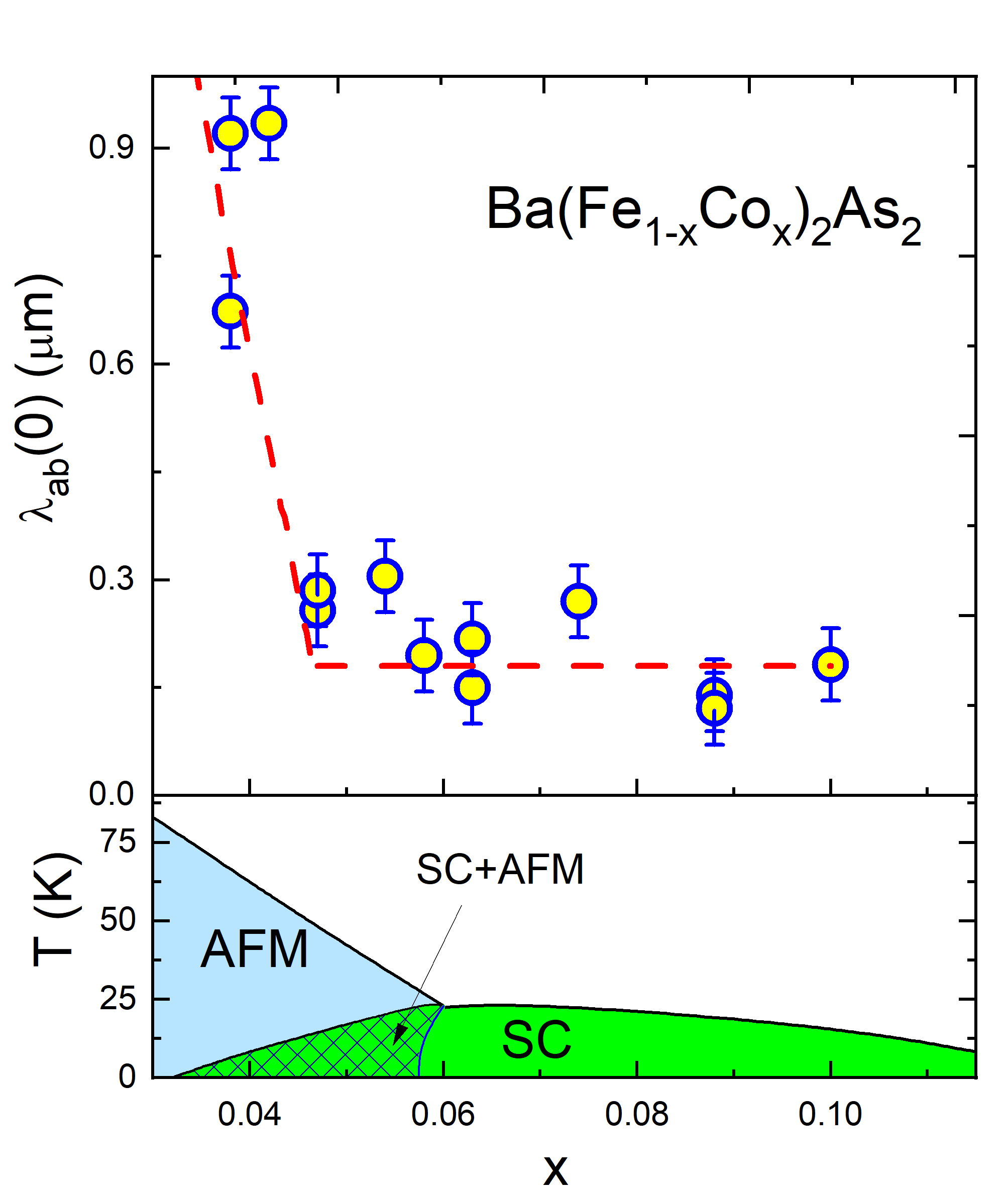
Later these measurements were extended to Ba(Fe1-xCox)2As2 (BaCo122), where the phase diagram is traversed by electron doping with Co, as opposed to the isoelectric P/As substitution in BaAsP122. This charge doping introduces considerable disorder so in this case quantum oscillations could not be observed. The BaCo122 data show a similar peak in at the QCP (figure 21) but the higher scatter of the data and the strong increase in inside the region of the phase diagram where superconductivity coexists with antiferromagnetism makes the peak more difficult to discern Alcoating Also, it is important to emphasize that in order to observe a sharp QCP-related peak, several samples of finely spaced compositions are required. The usual case for such compounds is a mismatch between the nominal and actual composition, making such experiments very challenging.
Within conventional theory, a peak in should cause a corresponding decrease in the lower critical field . However, in BaAsP122 the opposite was found at the QCP putzke . This increase of was attributed to an anomalous increase in the vortex core energy at the QCP putzke . Measurements of in BaCo122 showed the opposite behavior: a clear decrease of at the QCP Joshi2020 . This dichotomy calls for further measurements of and by different methods on clean systems and those where disorder is added in a controlled way.
12 Concluding remarks
This paper presents some highlights from our research using tunnel diode resonators. There is every reason to believe that this technique will continue to be refined and used to explore new forms of superconductivity. Our approach was inspired by a Cornell low temperature group seminar given many years earlier. One prevailing philosophy in that group was the importance of building a unique kind of apparatus with very high sensitivity. To those of us who were graduate students, the discovery of superfluidity in 3He by Osheroff, Richardson and Lee brought that lesson home in a particularly forceful way. In effect, a Nobel prize hinged on the appearance of a tiny glitch in the 3He pressurization curve. Of course, you had to be cold enough to see it! A later unexpected jump in the frequency of a torsion oscillator lead to the identification of the Kosterlitz-Thouless transition in 4He films by David Bishop and John Reppy. This was a seminal discovery in the physics of topological matter. RWG is grateful to Dave Lee, John Reppy, Bob Richardson and all the other inhabitants of H-corridor for their insights, camraderie and inspiration during those fantastic years.
Acknowledgements.
R.P. is supported by the U.S. Department of Energy (DOE), Office of Science, Basic Energy Sciences, Materials Science and Engineering Division. Ames Laboratory is operated for the U.S. DOE by Iowa State University under contract DE-AC02-07CH11358. AC is supported by UK EPSRC grant EP/R011141/1. RWG was supported by DOE award DE-AC0298CH1088 (Center for Emergent Superconductivity) and National Science Foundation award numbers NSF-DMR91-20000 and NSF-DMR-05-03882.Conflict of interest
The authors declare that they have no conflict of interest.
References
- (1) J.C. Bednorz and K.A. Muller, Z. Phys. B. - Condensed Matter 64, 189 (1986).
- (2) J. Bardeen, L.N. Cooper, J.R. Schrieffer, Phys. Rev. 108, 1175 (1957).
- (3) M. Sigrist and K. Ueda, Rev. Mod. Phys. 63, 239 (1991).
- (4) For a review, see D.J. Scalapino, Jour. Low Temp. Phys. 117, Nos. 3/4, 179 (1999).
- (5) J.F. Annett, N. Goldenfeld, S.R. Renn, chapter 9, in , (New Jersey, World Scientific) ed. D.M. Ginsberg (1990)
- (6) K.A. Moler, D.J. Baar, J.S. Urbach, R. Liang, W.N. Hardy, A. Kapitulnik, Phys. Rev. Lett. 73, 2744 (1994).
- (7) W.N. Hardy, D.A. Bonn, D.C. Morgan, R.X. Liang, K. Zhang, Phys. Rev. Lett. 70, 3999 (1993).
- (8) M. Tinkham, , 2nd edition, (Dover, 1996).
- (9) R. Prozorov and R. W. Giannetta, Supercond. Sci. Techn. 19, R41 (2006).
- (10) D.A. Wollman, D.J. van Harlingen, W.C. Lee, D.M. Ginsberg, A.J. Leggett, Phys. Rev. Lett. 71, 2134 (1993).
- (11) C.C. Tsuei, J.R. Kirtley, C.C. Chi, L.S. Yu-Jahnes, A. Gupta, T. Shaw, J.Z. Sun, M.B. Ketchum, Phys. Rev. Lett. 73, 593 (1994).
- (12) V. G. Kogan and R. Prozorov, Phys. Rev. B 103, 054502 (2021).
- (13) B.S. Chandrasekhar and D. Einzel, Ann. Phys. Lpz. 2 535 (1993).
- (14) D. Xu, S. K. Yip, and J. A. Sauls, Phys. Rev. B 51, 16 233, (1995).
- (15) S.K. Yip and J.A. Sauls, Phys. Rev. Lett. 69, 2264 (1992).
- (16) C.T. Van Degrift, Rev. Sci. Instrum. 46, 599 (1975).
- (17) R. Prozorov, R.W. Giannetta, A. Carrington and F.M. Araujo-Moreira, Phys. Rev. B 62, 115 (2000).
- (18) R. Prozorov, arXiv:2105.00998 (2021).
- (19) O. Heybey, Master’s thesis, Cornell University (1962) (unpublished).
- (20) C. Boghosian, H. Meyer, J. Rives, Phys. Rev. 146, 110 (166).
- (21) P.M. Tedrow, G. Faraci, R. Meservey, Jour. Appl. Phys. 74 2028 (1969).
- (22) A. Carrington, R. W. Giannetta, J. T. Kim, and J. Giapintzakis, Phys. Rev. B 59, R14173(R) (1999)
- (23) A.Carrington, I.J. Bonalde, R. Prozorov, R.W. Giannetta, A.M. Kini, J. Schlueter, H.H. Wang, U. Geiser, J.M. Williams, Phys. Rev. Lett. 83 4172 (1999).
- (24) H.Kim, M. Tanatar, R. Prozorov, Rev. Sci. Instr. 89, 094704 (2018).
- (25) I. Bonalde, B.D. Yanoff, M.B. Salamon, D.J. Van Harlingen, E.E.M. Chia, Z.Q. Mao, Y. Maeno, Phys. Rev. Lett. 85, 4775 (2000).
- (26) I. Bonalde, B.D. Yanoff, M.B. Salamon, E.E.M. Chia, Phys. Rev. B 67 012506 (2003).
- (27) J.D. Fletcher, A. Carrington, P. Diener, P. Rodiere, J. P. Brison, R. Prozorov, T. Olheiser and R.W. Giannetta, Phys. Rev. Lett. 98, 057003 (2007).
- (28) J.D. Fletcher, A. Serafin, L. Malone, J. G. Analytis, J -H. Chu, A. S. Erickson, I. R. Fisher and A. Carrington, Phys. Rev. Lett. 102, 147001 (2009).
- (29) A.M. Campbell, J. Phys. C: Solid State Phys.2, 1492 (1969).
- (30) A.M. Campbell, J. Phys. C: Solid State Phys.4, 3186 (1971).
- (31) R. Prozorov, R.W. Giannetta, N. Kameda, T. Tamegai, J.A. Schlueter, P. Fournier, Phys. Rev. B 67, 184501 (2003).
- (32) D.H. Wu and S. Sridhar, Phys. Rev. Lett. 65, 2074 (1990).
- (33) N.H. Tea, F.A.B. Chaves, U. Klostermann, R.W. Giannetta, M.B. Salamon, J.M. Williams, H.H. Wang, U. Geiser, Physica C 280, 281 (1997).
- (34) R.Willa, V.B. Geshkenbein and G. Blatter, Phys. Rev. B 93 064515 (2016).
- (35) C.P. Bidnosti, W.N. Hardy, D.A. Bonn, R. Liang, Phys. Rev. Lett. 83, 3277 (1999).
- (36) S. Sridhar, D.H. Wu, W. Kennedy, Phys. Rev. Lett. 63, 1873 (1989)
- (37) A. Maeda, Y. Iino, T. Hanaguri, N. Motohira, K. Kishio, T. Fukase, Phys. Rev. Lett. 74, 1202 (1995).
- (38) J. A. Wilcox, M. J. Grant, L. Malone, C. Putzke, D. Kaczorowski, T. Wolf, F. Hardy, C. Meingast, J.G. Analytis, J.-H. Chu, I. R. Fisher, A. Carrington, arXiv:2008.04050.
- (39) C.-R. Hu, Phys. Rev. Lett. 72, 1526 (1994).
- (40) Y. Tanaka and S. Kashiwaya, Phys. Rev. Lett. 74, 3451 (1995).
- (41) M. Fogelstrom, D. Rainer, J.A. Sauls, Phys. Rev. Lett. 79, 281 (1997).
- (42) Y.S. Barash, M.S. Kalenkov, J. Kurkijarvi, Phys. Rev. B 62, 6665 (2000).
- (43) R. Prozorov, R.W. Giannetta, P. Fournier, R.L. Greene, Phys. Rev. Lett. 85, 3700 (2000).
- (44) A. Carrington, F. Manzano, R. Prozorov, R.W. Giannetta, N. Kameda, T. Tamegai, Phys. Rev. Lett. 86, 1074 (2001).
- (45) H. Walter, W. Prusseit, R. Semerand, H. Kinder, W. Assmann, H. Huber, H. Burkhardt, D. Rainer, J.A. Sauls, Phys. Rev. Lett. 80, 3598 (1998).
- (46) where = and is the angle between the surface normal and the [110] axis.
- (47) Shan-Wen Tsai and P.J. Hirschfeld, Phys. Rev. Lett 89, 147004 (2002).
- (48) D.A. Bonn, S. Kamal, A. Bonakdarpour, R. Liang, W.N. Hardy, C.C. Homes, D.N. Basov, T. Timusk, Czech. J. Phys. 46, 3195 (1996).
- (49) Y. Kamihara, T. Watanabe, M. Hirano, H. Hosoan, J. Am. Chem. Soc. 130, 3296 (2008).
- (50) I.I. Mazin, D.J. Singh, M.D. Johannes, M.H. Du, Phys. Rev. Lett. 101, 057003 (2008).
- (51) P.J. Hirschfeld, M.M. Korshunov and I.I. Mazin, Rep. Prog. Phys. 74, 124508 (2011).
- (52) J.D. Fletcher, A. Carrington, O.J. Taylor, S.M. Kazakov, J. Karpinski, Phys. Rev. Lett. 95, 097005 (2005).
- (53) H. Kim, K. Cho, M. A. Tanatar, V. Taufour, S. K. Kim, S. L. Bud’ko, P. C. Canfield, V. G. Kogan, and R. Prozorov, Symmetry (Basel). 11, 1012 (2019).
- (54) K. Cho, A. Fente, S. Teknowijoyo, M. A. Tanatar, K. R. Joshi, N. M. Nusran, T. Kong, W. R. Meier, U. Kaluarachchi, I. Guillamón, H. Suderow, S. L. Bud’ko, P. C. Canfield, and R. Prozorov, Phys. Rev. B 95, 100502 (2017). doi:10.1103/PhysRevB.95.100502.
- (55) K. R. Joshi, N. M. Nusran, M. A. Tanatar, K. Cho, W. R. Meier, S. L. Bud’ko, P. C. Canfield, and R. Prozorov, Phys.Rev. Appl. 11, 014035 (2019). doi:10.1103/PhysRevApplied.11.014035.
- (56) V. G. Kogan, C. Martin, and R. Prozorov, Phys. Rev. B 80, 14507 (2009). doi:10.1103/PhysRevB.80.014507.
- (57) R. Prozorov and V.G. Kogan, Rep. Prog. Phys. 74 124505 (2011).
- (58) P.W. Anderson, J. Phys. Chem. Sol. 11, 26 (1959).
- (59) Y. Bang, Eur. Phys. Lett. 86, 47001 (2009).
- (60) A.B. Vorontsov, M.G. Vavilov and A.V. Chubukov, Phys. Rev. B 79, 140507 (2009).
- (61) P.J. Hirschfeld and N. Goldenfeld, Phys. Rev. B 48, 4219 (1993).
- (62) V. G. Kogan and R. Prozorov, Phys. Rev. B 93, 224515 (2016).
- (63) H. Kim, R.T. Gordon, M.A. Tanatar, J. Hua, U. Welp, W.K. Kwok, N. Ni, S.L. Bud’ko, P.C. Canfield, A.B. Vorontsov and R. Prozorov, Phys. Rev. B 82, 060518 (2010).
- (64) E. I. Timmons, S. Teknowijoyo, M. Końńczykowski, O. Cavani, M. A. Tanatar, S. Ghimire, K. Cho, Y. Lee, L. Ke, N. H. Jo, S. L. Bud’ko, P. C. Canfield, P. P. Orth, M. S. Scheurer, and R. Prozorov, Phys. Rev. Research 2, 023140 (2020).
- (65) R. Prozorov, R.W. Giannetta, A. Carrington, P. Fournier, R.L. Greene, P. Guptsarma, D.G. Hinks, A.R. Banks, Appl. Phys. Lett. 77, 4202 (2000).
- (66) R. Meservey and P.M. Tedrow, Jour. Appl. Phys. 40, 2028 (1969).
- (67) K. Hashimoto, K. Cho, T. Shibauchi, S. Kasahara, Y. Mizukami, R. Katsumata, Y. Tsuruhara, T. Terashima, H. Ikeda, M. A. Tanatar, H. Kitano, N. Salovich, R. W. Giannetta, P. Walmsley, A. Carrington, R. Prozorov, and Y. Matsuda, Science (80) 336, 1554 (2012). doi:10.1126/science.1219821.
- (68) P. Walmsley, C. Putzke, L. Malone, I. Guillamón, D. Vignolles, C. Proust, S. Badoux, A.I. Coldea, M.D. Watson, S. Kasahara, Y. Mizukami, T. Shibauchi, Y. Matsuda, and A. Carrington, Phys. Rev. Lett. 110, 257002 (2013). DOI:10.1103/PhysRevLett.110.257002.
- (69) A. J. Leggett Phys. Rev. 140, A1869 (1965). doi:10.1103/PhysRev.140.A1869.
- (70) A. Levchenko, M.G. Vavilov, M. Khodas, and A.V. Chubukov, Phys. Rev. Lett. 110, 177003 (2013). DOI:10.1103/PhysRevLett.110.177003.
- (71) T. Nomoto and H. Ikeda, Phys. Rev. Lett. 111, 167001 (2013).
- (72) C. Putzke, P. Walmsley, J.D. Fletcher, L. Malone, D. Vignolles, C. Proust, S. Badoux, P. See, H.E. Beere, D.A. Ritchie, S. Kasahara, Y. Mizukami, T. Shibauchi, Y. Matsuda and A. Carrington, Nature comm. 5, 5679 (2014).DOI: 10.1038/ncomms6679.
- (73) K. R. Joshi, N. M. Nusran, M. A. Tanatar, K. Cho, S. L. Bud’ko, P. C. Canfield, R. M. Fernandes, A. Levchenko, and R. Prozorov, New J. Phys. 22, 053037 (2020). doi:10.1088/1367-2630/ab85a9.