Self-Training with Differentiable Teacher
Abstract
Self-training achieves enormous success in various semi-supervised and weakly-supervised learning tasks. The method can be interpreted as a teacher-student framework, where the teacher generates pseudo-labels, and the student makes predictions. The two models are updated alternatingly. However, such a straightforward alternating update rule leads to training instability. This is because a small change in the teacher may result in a significant change in the student. To address this issue, we propose DRIFT, short for differentiable self-training, that treats teacher-student as a Stackelberg game. In this game, a leader is always in a more advantageous position than a follower. In self-training, the student contributes to the prediction performance, and the teacher controls the training process by generating pseudo-labels. Therefore, we treat the student as the leader and the teacher as the follower. The leader procures its advantage by acknowledging the follower’s strategy, which involves differentiable pseudo-labels and differentiable sample weights. Consequently, the leader-follower interaction can be effectively captured via Stackelberg gradient, obtained by differentiating the follower’s strategy. Experimental results on semi- and weakly-supervised classification and named entity recognition tasks show that our model outperforms existing approaches by large margins.
1 Introduction
Self-training is a classic method that was first proposed for semi-supervised learning Rosenberg et al. (2005); Lee (2013). It is also interpreted as a regularization method Mobahi et al. (2020), and is extended to weakly-supervised learning and domain adaptation Meng et al. (2018). The approach has gain popularity in many applications. For example, in conjunction with pre-trained language models Devlin et al. (2019), self-training has demonstrated superior performance on tasks such as natural language understanding Du et al. (2021), named entity recognition Liang et al. (2020), and question answering Sachan and Xing (2018).
Conventional self-training can be interpreted as a teacher-student framework. Within this framework, a teacher model generates pseudo-labels for the unlabeled data. Then, a student model updates its parameters by minimizing the discrepancy between its predictions and the pseudo-labels. The teacher subsequently refines its parameters based on the updated version of the student using pre-defined rules. Such rules include minimizing a loss function Pham et al. (2020), copying the student’s parameters Rasmus et al. (2015), and integrating models from previous iterations (Laine and Aila, 2017; Tarvainen and Valpola, 2017). The above procedures are operated iteratively.
Computationally, the alternating update procedure often causes training instability. Such instability comes from undesired interactions between the teacher and the student. In practice, we often use stochastic gradient descent to optimize the student, and the noise of the stochastic gradient can cause oscillation during training. This means in a certain iteration, the student is optimized towards a certain direction; while in the next iteration, it may be optimized toward a drastically different direction. Such a scenario renders the optimization ill-conditioned. Moreover, the student model’s gradient is determined by the pseudo-labels generated by the teacher. Because of the training instability, a small change in the pseudo-labels may result in a substantial change in the student.
To resolve this issue, we propose DRIFT (differentiable self-training), where we formulate self-training as a Stackelberg game Von Stackelberg (2010). The concept arises from economics, where there are two players, called the leader and the follower. In a Stackelberg game, the leader is always in an advantageous position by acknowledging the follower’s strategy. Within the self-training framework, we grant the student a higher priority than the teacher. This is because the teacher serves the purpose of generating intermediate pseudo-labels, such that the student can behave well on the task. The student (i.e., the leader) procures its advantage by considering what the response of the teacher (i.e., the follower) will be, i.e., how will the follower react after observing the leader’s move. Then, the leader makes its move, in anticipation of the predicted response of the follower. We remark that the Stackelberg game formulation has also been used in other domains such as adversarial training (Zuo et al., 2021).
We highlight that in DRIFT, the student has a higher priority than the teacher. In contrast, in conventional self-training, the two models are treated equally and have the same priority. When using conventional self-training, the student only reacts to what the teacher has generated. In differentiable self-training, the student recognizes the teacher’s strategy and reacts to what the teacher is anticipated to response. In this way, we can find a better descent direction for the student, such that training can be stabilized.
To facilitate the leader’s advantage, our framework treats the follower’s strategy (i.e., pseudo-labels generated by the teacher) as a function of the leader’s decision (i.e., the student’s parameters). In this way, differentiable self-training can be viewed solely as a function of the student’s parameters. Therefore, the problem can be efficiently solved using gradient descent.
Besides pseudo-labels, the teacher can also generate sample weights Freund and Schapire (1997); Kumar et al. (2010); Malisiewicz et al. (2011). Sample reweighting associates low-confidence samples with small weights, such that the influence of noisy labels can be effectively reduced. Similar to pseudo-labels, sample weights and the student model are also updated iteratively. As such, we can further equip DRIFT with differentiable sample weights. This can be achieved by integrating the weights as a part of the follower’s strategy. We remark that our method is flexible and can incorporate even more designs to the follower’s strategy.
We evaluate the performance of differentiable self-training on a set of weakly- and semi-supervised text classification and named entity recognition tasks. In some weakly-supervised learning tasks, our proposed method achieves competitive performance in comparison with fully-supervised models. For example, we obtain a 97.3% vs. 96.2% classification accuracy on Yelp, and we do not use any labeled training data from the Yelp dataset.
We highlight that our proposed differentiable self-training approach is an efficient substitution to existing self-training methods. Moreover, our method does not introduce any additional tuning parameter to the teacher-student framework. Additionally, DRIFT is flexible and can combine with various neural architectures. We summarize our contributions as the following: (1) We propose a differentiable self-training framework DRIFT, which employs a Stackelberg game formulation of the teacher-student approach. (2) We employ differentiable pseudo-labels and differentiable sample weights as the follower’s strategy. Our method alleviates the training instability issue. (3) Extensive experiments on semi-supervised node classification, semi- and weakly-supervised text classification and named entity recognition tasks verify the efficacy of DRIFT.
2 Background
Self-training for semi-supervised learning. Self-training is one of the earliest and simplest approaches to semi-supervised learning Rosenberg et al. (2005); Lee (2013). The method uses a teacher model to generate new labels, on which a student model is fitted. Similar methods such as self-knowledge distillation Furlanello et al. (2018) are proposed for supervised learning. The major drawback of self-training is that it is vulnerable to label noise. A popular approach to tackle this is sample reweighting Freund and Schapire (1997); Kumar et al. (2010); Malisiewicz et al. (2011), where high-confidence samples Rosenberg et al. (2005); Zhou et al. (2012) are assigned larger weights. Data augmentation methods Berthelot et al. (2019); Chen et al. (2020) are also proposed to further enhance self-training.
Self-training for weakly-supervised learning. Weak supervision sources, such as semantic rules and knowledge bases, facilitate generating large amounts of labeled data Goh et al. (2018); Hoffmann et al. (2011). The weak supervision sources have limited coverage, i.e., not all samples can be matched by the rules, such that a considerable amount of samples are unlabeled. Moreover, the generated weak labels usually contain excessive noise. Recently, self-training techniques are adopted to weakly-supervised learning. In conjunction with pre-trained language models Devlin et al. (2019); Liu et al. (2019), the technique achieves superior performance in various tasks Meng et al. (2018, 2020); Niu et al. (2020); Liang et al. (2020); Yu et al. (2021).
3 Method
For both semi-supervised and weakly-supervised learning problems, we have labeled samples and unlabeled samples . Here is the number of labeled data, and is the number of unlabeled data. Note that in weakly-supervised learning, we have unlabeled data because of the limited coverage of weak supervision sources. The difference between semi- and weakly-supervised learning is that in the former case, the labels are assumed to be accurate, whereas in the latter case, the labels are noisy. The goal is to learn a classifier , where denotes all the data samples, is the label set, and is the number of classes. The classifier outputs a point in the -dimensional probability simplex, where each dimension denotes the probability that the input belongs to a specific class.
3.1 Differentiable Self-Training for Semi-Supervised Learning
Self-training can be interpreted as a teacher-student framework. Within this framework, the teacher first generates pseudo-labels (see (6)) for the data samples. Then, the student updates itself by minimizing a loss function (see (8)), subject to the generated pseudo-labels. Such two procedures are run iteratively.
We remark that self-training behaves poorly when encountering unreliable pseudo-labels, which will cause the student model to be updated towards the wrong direction. To alleviate this issue, we find a good initialization for the models. In semi-supervised learning, is found by fitting a model on the labeled data . Concretely, we solve
| (1) |
Here , and is the supervised loss, e.g., the cross-entropy loss. (1) can be efficiently optimized using stochastic gradient-type algorithms, such as Adam Kingma and Ba (2015).
At time , denote the student’s parameters , and the teacher’s parameters . We set both the student’s and the teacher’s initial parameters to , i.e., . Note that the teacher model depends on the student. We adopt an exponential moving average Laine and Aila (2017); Tarvainen and Valpola (2017) approach to model such a dependency:
| (2) |
Recall that in our differentiable self-training framework, the student acknowledges the teacher’s strategy. This meets the definition of a Stackelberg game Von Stackelberg (2010), and we propose the following formulation:
| (3) | ||||
Here recall that is the unlabeled data samples, and is the size of . In (3), is the teacher’s strategy, which contains differentiable pseudo-labels (i.e., in (6)) and differentiable sample weights (i.e., in (7)). The loss function is defined in (8). Note that we still include the supervised loss in (1) in the objective function . Following conventions, in (3), the minimization problem solves for the leader, and we call the follower’s strategy. Note that the Stackelberg game formulation (3) has also been adopted in adversarial training (Zuo et al., 2021).
The Stackelberg game formulation is fundamentally different from conventional self-training approaches, where the teacher is not treated as a function of the student . In our differentiable self-training framework, the leader takes the follower’s strategy into account by considering . In this way, self-training can be viewed solely in terms of the leader’s parameters .
Consequently, the leader problem can be efficiently solved using stochastic gradient-type algorithms, where the gradient is
| (4) | ||||
In (4)111The “leader” term is written as instead of because the partial derivative is only taken with respect to the third argument in . We drop the term in to avoid causing confusion., we have because of (2). Note that a conventional self-training method only considers the “leader” term, and ignores “leader-follower interaction”. This causes training instabilities, which we demonstrate empirically in Fig. 1 and Fig. 2.
The proposed differential self-training algorithm is summarized in Algorithm 1. In the next two sections, we spell out the two components of the follower’s strategy, namely differentiable pseudo-labels and differentiable sample weights.
3.2 Differentiable Pseudo-Labels
In a self-training framework, the teacher model labels the unlabeled data. Concretely, at time , for each sample in the unlabeled dataset, a hard pseudo-label (Lee, 2013) is defined as
| (5) |
Here is in the probability simplex, and denotes its -th entry.
There are two problems with the hard pseudo-labels. First, differentiable self-training requires every component of the follower’s strategy (3) to be differentiable with respect to the leader’s parameters. However, (5) introduces a non-differentiable operation. Second, the hard pseudo-labels exacerbates error accumulation. This is because only contains information about the most likely class, such that statistics regarding the prediction confidence is lost. For example, suppose in a two-class classification problem, we obtain for some . This prediction result indicates that the model is uncertain to which class belongs. However, under the hard pseudo-label , the student model becomes unaware of such uncertainty.
To resolve the above two issues, we propose to employ soft pseudo-labels Xie et al. (2016, 2020); Meng et al. (2020). Concretely, for a data sample in a batch , the -th entry of its soft pseudo-label is defined as
| (6) |
where , and is a temperature parameter that controls the “softness” of the soft pseudo-label. Note that when the temperature is low, i.e., , the soft pseudo-label becomes sharper and eventually converges to the hard pseudo-label (5).
In (6), the soft pseudo-label is a function of the teacher’s parameters , which in turn is a function of the student’s parameters (2). Therefore, is differentiable with respect to , and fits in the differentiable self-training framework. The gradient of with respect to can be efficiently computed by a single back-propagation using deep learning libraries.
Notice that (6) emphasizes the tendency of belonging to a specific class, instead of to which class belongs. Therefore, even when is wrong, the soft version of it is still informative.
3.3 Differentiable Sample Weights
Sample reweighting is an effective tool to tackle erroneous labels Freund and Schapire (1997); Kumar et al. (2010); Malisiewicz et al. (2011); Liang et al. (2020). Specifically, pseudo-labels that have dominating entries are more likely to be accurate than those with uniformly distributed entries. For example, a sample labeled is more likely to be classified correctly than a sample labeled . With this intuition, for a sample and its soft pseudo-label , we define its sample weight as
| (7) |
where is the entropy of that satisfies . Note that if the pseudo-label is uniformly distributed, then the corresponding sample weight is low, and vice versa. Similar to the pseudo-label , the sample weight is a function of the teacher’s parameters , and further a function of the student’s parameters .
With the differentiable pseudo-labels and the differentiable sample weights, we define the student’s loss function as
| (8) |
where is the Kullback–Leibler (KL) divergence.
3.4 Weakly-Supervised Learning
Recall that in weakly-supervised learning, we have both labeled data and unlabeled data . Note that weak supervision sources often yield noisy labels. This is because data are annotated automatically by, for example, linguistic rules, which have limited accuracy. As such, the supervised loss in (3) only exacerbates the label noise issue.
We address this problem by discarding the noisy weak labels in after obtaining the initialization (1). Accordingly, we adopt the following formulation for weakly-supervised learning:
| (9) | ||||
Here is the total number of training samples. Note that in comparison with (3), we drop the supervised loss . Moreover, the teacher model now generates soft pseudo-labels for all the data, instead of only the data in .
4 Experiments
We conduct two sets of experiments: weakly- and semi-supervised text classification. We also examine semi-supervised node classification on graphs (Appendix A). All the results have passed a paired t-test with . When using pre-trained language models, we employ a RoBERTa-base Liu et al. (2019) model obtained from the HuggingFace Wolf et al. (2019) codebase. We implement all the methods using PyTorch (Paszke et al., 2019), and experiments are run on NVIDIA 2080Ti GPUs. All the training details are deferred to the appendix.
| Dataset | AGNews | IMDB | Yelp | MIT-R | CoNLL-03 | Webpage | BC5CDR | Wikigold |
| RoBERTa-Full | 91.41 | 94.26 | 97.27 | 88.51 | 90.11 (89.14/91.10) | 72.39 (66.29/79.73) | 85.15 (83.74/86.61) | 86.43 (85.33/87.56) |
| RoBERTa-Weak | 82.25 | 72.60 | 79.91 | 70.95 | 75.61 (83.76/68.90) | 59.11 (60.14/58.11) | 78.51 (74.96/82.42) | 51.55 (49.17/54.50) |
| WeSTClass | 82.78 | 77.40 | 76.86 | --- | --- | --- | --- | --- |
| Self-training | 86.07 | 85.72 | 89.95 | 73.59 | 77.28 (83.42/71.98) | 56.90 (54.32/59.74) | 79.92 (74.73/85.90) | 56.90 (54.32/59.74) |
| UAST | 86.28 | 84.56 | 90.53 | 74.41 | 77.92 (83.30/73.20) | 58.18 (56.33/60.14) | 81.50 (80.09/82.98) | 57.79 (52.64/64.05) |
| BOND | 86.19 | 88.36 | 93.18 | 75.90 | 81.48 (82.05/80.92) | 65.74 (67.37/64.19) | 81.53 (79.54/83.63) | 60.07 (53.44/68.58) |
| DRIFT | 87.80 | 91.56 | 96.24 | 77.15 | 81.74 (81.45/82.02) | 66.04 (65.23/66.87) | 82.62 (82.57/82.68) | 60.66 (57.50/64.21) |
4.1 Warmup: TwoMoon Experiments
To understand the efficacy of DRIFT, we conduct a semi-supervised classification experiment on a classic synthetic dataset “TwoMoon”. The dataset contains two classes, and for each class we generate labeled samples and unlabeled ones.
We compare DRIFT with conventional Self-training. The only difference between the two methods is that DRIFT adopts the differentiable strategies, while Self-training does not. In both methods, the teacher/student model is a two-layer feed-forward neural network, with hidden dimension and (hyperbolic tangent) as the non-linearity. We first train the models for epochs using the labeled samples. We then conduct self-training with learning rate 0.01 and Adam (Kingma and Ba, 2015) as the optimizer. We adopt an exponential moving average approach (2) with , and we set the temperature parameter for the soft pseudo-labels (6).
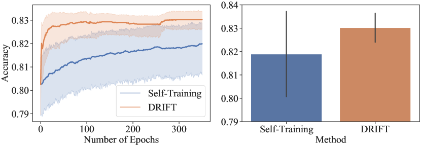
We conduct trails, and Fig. 1 shows the accuracy and the variance during training. We can see that Self-training yields a much larger variance, indicating an unstable training process. Note that the performance gain of DRIFT to Self-training has passed a paired-student t-test with p-value .
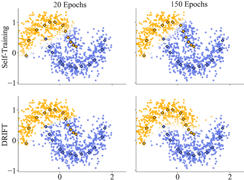
Moreover, by examining the experimental results, we find that Self-training at times gets stuck at subpotimal solutions. As an example, in Fig. 2, notice that the two methods behave equally well at epoch 20. However, Self-training gets stuck and does not improve at epoch 150. This is because the teacher generates hazardous labels that avert the student from improving. Meanwhile, by incorporating differentiable strategies, the performance of DRIFT improves at epoch 150 from epoch 20.
4.2 Weakly-Supervised Text Classification
We fine-tune a pre-trained RoBERTa model for weakly-supervised learning. In addition, we demonstrate that our method works well when trained-from-scratch and when using different backbones than the Transformer Vaswani et al. (2017). See Section 4.3 and Table 3 for details.
Settings. We use the following datasets: Topic Classification on AGNews Zhang et al. (2015); Sentiment Analysis on IMDB Maas et al. (2011) and Yelp Meng et al. (2018); Slot Filling on MIT-R Liu et al. (2013); and Named Entity Recognition (NER) on CoNLL-03 Tjong Kim Sang (2002), Webpage Ratinov and Roth (2009), Wikigold Balasuriya et al. (2009), and BC5CDR Li et al. (2016). The dataset statistics are summarized in Table 7. For each dataset, we generate weak labels using some pre-defined rules, after which the same data and generated weak labels are used by all the methods. More details about the weak supervision sources are in Appendix C.
We adopt several baselines:
-
•
RoBERTa Liu et al. (2019) uses the RoBERTa-base model with task-specific classification heads.
- •
-
•
WeSTClass Meng et al. (2018) leverages generated pseudo-documents and uses self-training to bootstrap over all the samples.
-
•
BOND Liang et al. (2020) uses a teacher-student framework for self-training. The teacher model is periodically updated to generate pseudo-labels when training the student.
- •
Recall that for weakly-supervised learning, we first fine-tune a RoBERTa model using the weakly-labeled data, and then we discard the weak labels and continue with self-training. This is an effective strategy to reduce overfitting on label noise (Yu et al., 2021). We follow this procedure for both DRIFT and all the baseline methods.
Results. Experimental results are summarized in Table 1. We can see that DRIFT achieves the best performance in all the tasks. Notice that the baselines that adopt self-training, e.g., WestClass, Self-training, UAST, and BOND, outperform the vanilla RoBERTa-Weak method. This is because in weakly-supervised learning, a noticeable amount of labels are inaccurate. Therefore, without noise suppressing approaches such as self-training, models cannot behave well. However, without taking the teacher’s strategy into account, these methods still suffer from training instabilities, such that they are not as effective as DRIFT.
We highlight that on some datasets, performance of our method is close to the fully-supervised model RoBERTa-Full, even though we do not use any clean labels. For example, DRIFT achieves 91.6% vs. 94.3% performance on IMDB, 96.2% vs. 97.3% on Yelp, and 82.6 vs. 85.1 on BC5CDR.
4.3 Semi-Supervised Text Classification
| Dataset | AGNews | IMDB | Amazon | |||||||||
| Labels/class | 30 | 50 | 200 | 1000 | 30 | 50 | 200 | 1000 | 30 | 50 | 200 | 1000 |
| RoBERTa-Semi | 83.98 | 87.44 | 88.01 | 90.91 | 86.64 | 88.37 | 89.25 | 90.54 | 88.21 | 89.66 | 92.31 | 93.65 |
| VAMPIRE | --- | --- | 83.90 | 85.80 | --- | --- | 82.20 | 85.40 | --- | --- | --- | --- |
| UDA | 85.92 | 88.09 | 88.33 | 91.22 | 89.30 | 89.42 | 89.72 | 90.87 | --- | --- | --- | --- |
| MixText | 88.50 | 88.85 | 89.20 | 91.55 | 84.34 | 88.72 | 89.45 | 91.20 | --- | --- | --- | --- |
| Self-training | 84.62 | 88.04 | 88.67 | 91.47 | 88.13 | 88.80 | 89.84 | 91.04 | 89.92 | 90.55 | 92.55 | 93.83 |
| UAST | 87.74 | 88.65 | 89.21 | 91.81 | 89.21 | 89.56 | 90.11 | 91.48 | 91.27 | 91.50 | 92.68 | 93.97 |
| DRIFT | 89.46 | 89.67 | 90.17 | 92.47 | 89.77 | 90.03 | 90.83 | 92.39 | 91.82 | 92.67 | 93.16 | 94.28 |
| Dataset | AGNews | IMDB | ||||||||
| Labels per class | weak | 30 | 50 | 200 | 1000 | weak | 30 | 50 | 200 | 1000 |
| TextCNN | 79.45 | 78.81 | 79.98 | 85.46 | 86.78 | 82.44 | 63.32 | 66.61 | 73.22 | 78.29 |
| Self-training | 81.69 | 81.98 | 82.67 | 86.26 | 88.15 | 84.76 | 64.68 | 65.26 | 73.60 | 79.04 |
| UAST | 81.48 | 82.05 | 83.34 | 86.67 | 87.90 | 83.97 | 64.23 | 68.70 | 73.95 | 79.13 |
| DRIFT | 82.55 | 83.34 | 85.01 | 87.38 | 88.66 | 86.44 | 65.65 | 69.86 | 74.61 | 79.38 |
Datasets. We adopt AGNews, IMDB, and Amazon McAuley and Leskovec (2013) (see Table 7) in this set of experiments. For each dataset, we randomly sample data points from each class and annotate them with clean labels, while the other data are treated as unlabeled. Note that for all the splits of a particular dataset, we use the same development and test sets.
Settings. Our differentiable self-training framework works well in both fine-tuning and training-from-scratch regimes. Moreover, our approach is flexible to accommodate different neural architectures. We conduct two sets of experiments. In the first set, we fine-tune a pre-trained RoBERTa model, which uses the Transformer Vaswani et al. (2017) as its backbone. In the second set of experiments, we train a TextCNN (Kim, 2014) model from scratch, which employs a convolutional neural network as the foundation.
Baselines. Besides RoBERTa, Self-training, and UAST, which are used in weakly-supervised classification tasks, we adopt several new methods as baseline approaches.
-
•
VAMPIRE Gururangan et al. (2019) pre-trains a unigram document model on unlabeled data using a variational auto-encoder, and then uses its internal states as features for downstream applications.
-
•
UDA Xie et al. (2020) uses back translation and word replacement to augment unlabeled data, and forces the model to make consistent predictions on the augmented data to improve model performance.
-
•
MixText Chen et al. (2020) augments the training data by interpolation in the hidden space, and it exploits entropy and consistency regularization to further utilize unlabeled data during training.
Results. Experimental results are summarized in Table 2. We can see that DRIFT achieves the best performance across the three datasets under different setups. Notice that the performance of VAMPIRE is not satisfactory. This is because it does not use pre-trained models, unlike the other baselines. Pre-trained language models contain rich semantic knowledge, which can be effectively transferred to the target task and boost model performance. All the baselines do not explicitly consider the teacher’s strategy, and thus, they suffer from training instabilities.
We remark that UDA, UAST and MixText leverage external sources or data augmentation methods to make full use of the unlabeled data. These methods can potentially combine with DRIFT, which is of separate interests.
Fine-tuning vs. Training-from-scratch. Table 3 shows the results of training a TextCNN model from scratch. We can see that the model trained from scratch performs worse than fine-tuning a pre-trained model (Table 2). This is because TextCNN has significantly less parameters than RoBERTa, and is not pre-trained on massive text corpora. Therefore, we cannot take advantage of the semantic information from pre-trained models.
Nevertheless, under both weakly-supervised and semi-supervised learning settings, DRIFT consistently outperforms the baseline methods. This indicates that our method is architecture independent, and does not rely on transferring existing semantic information. As such, differentiable self-training serves as an effective plug-in module for existing models. We remark that DRIFT does not introduce any additional tuning parameter in comparison with conventional self-training.
4.4 Ablation Study
Components of DRIFT. We inspect different components of DRIFT, including the differentiable pseudo labels (DrPL), differentiable sample weights (DrW), and the sample reweighting strategy (SR)222For models without DrPL, we do not differentiate the pseudo-labels. For models without DrW, we still use (7) to perform sample rewriting, but we do not differentiate the weights, i.e., w/o DrW equals to w/ SR. For models without SR, we do not use sample reweighing.. Experimental results are summarized in Table 4. We observe that both differentiable pseudo-labels and differentiable sample weights contribute to model performance, as removing any of them hurts the classification accuracy. Also, DRIFT excels when the labels are noisy. We can see that our method brings 2.41% performance gain on average under the weakly-supervised setting, while it only promotes 1.08% average gain under the semi-supervised setting. Such results indicate that differentiable pseudo-labels and sample weight are effective in suppressing label noise.
| Method | AGNews | IMDB | ||||
| #labels | 30 | 1000 | weak | 30 | 1000 | weak |
| DRIFT | 89.46 | 92.47 | 87.80 | 89.77 | 92.39 | 91.56 |
| w/o DrPL | 87.63 | 92.11 | 86.13 | 89.05 | 91.75 | 86.78 |
| w/o DrW | 88.51 | 91.22 | 86.62 | 88.47 | 91.49 | 90.24 |
| w/o SR | 88.84 | 91.20 | 86.19 | 88.15 | 91.95 | 87.76 |
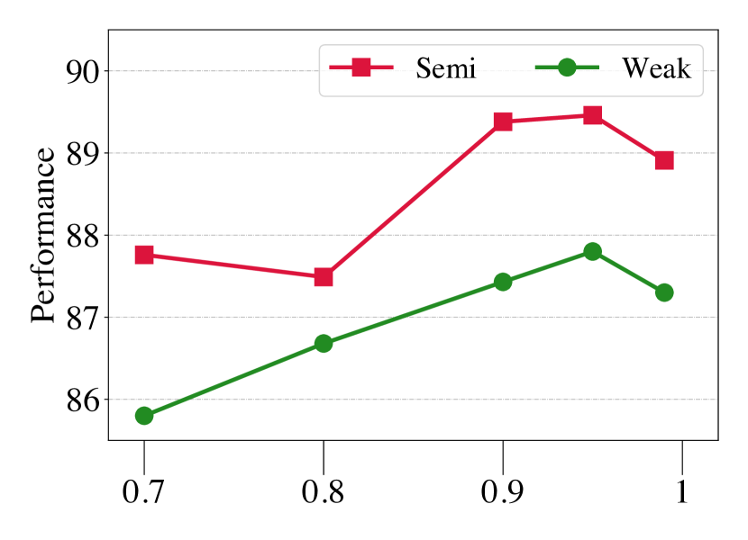
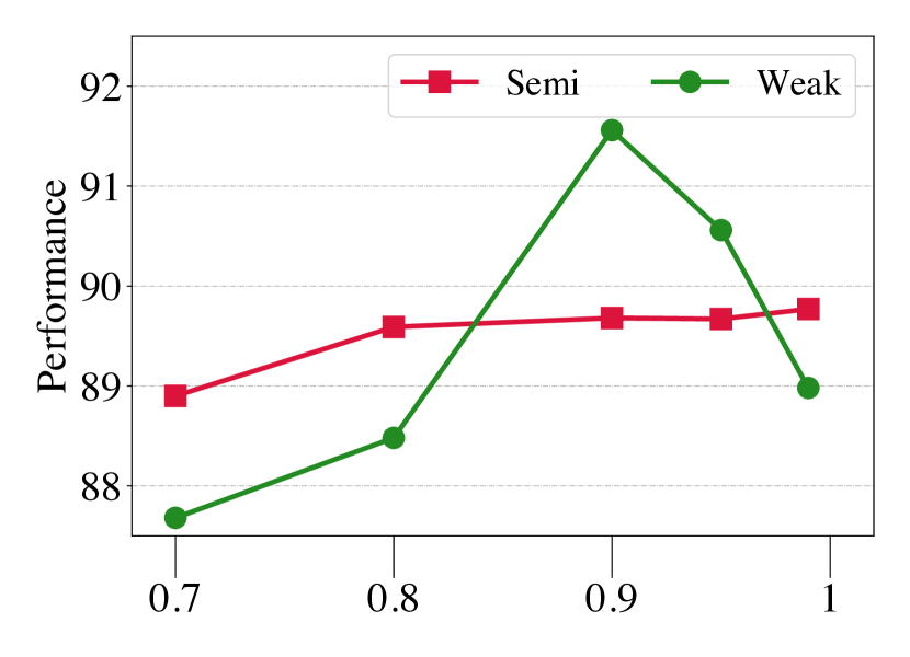
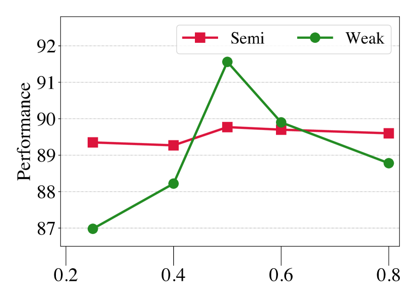
Sensitivity to hyper-parameters. We study models’ sensitivity to the exponential moving average rate and the soft pseudo-label’s temperature . Figure 3 shows the results. We can see that model performance peaks when is around . The teacher model updates too aggressively with a smaller (e.g., ), and too conservatively with a larger alpha (e.g., ). In the first case, the generated pseudo-labels are not reliable; and in the second case, model improves too slow. Also notice that the semi-supervised model is not sensitive to the temperature parameter. The weakly-supervised model achieves the best performance when . Note that a smaller essentially generates hard pseudo-labels, which drastically hurts model performance.
4.5 Case Study
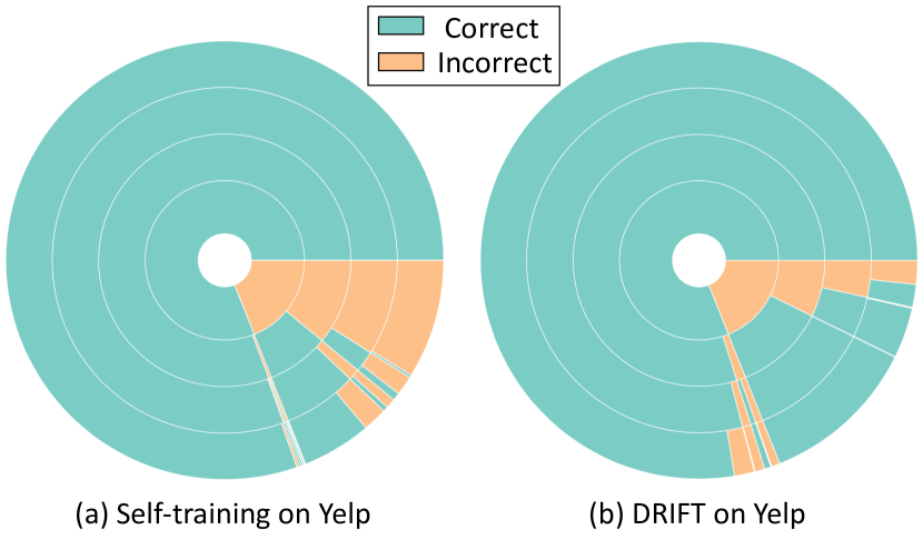
Figure 4 demonstrates error reduction. Samples are indicated by radii of the circle, and classification correctness is indicated by color. For example, if a radius has color orange, blue, blue, blue, then it is mis-classified at iteration 0, and correctly classified at iteration 100, 200, and 300. We can see that Self-training suffers from error accumulation, as around 2% more samples are mis-classified between iteration 200 and 300. In contrast, in DRIFT, a noticeable amount of incorrect predictions are rectified, and the accuracy improves by more than 15% after 300 iterations.
5 Discussion and Conclusion
In this paper, we propose a differentiable self-training framework, DRIFT, which formulates the teacher-student framework in self-training as a Stackelberg game. The formulation treats the student as the leader, and the teacher as the follower. In DRIFT, the student is in an advantageous position by recognizing the follower’s strategy. In this way, we can find a better descent direction for the student and can stabilize training. Empirical results on weakly- and semi-supervised natural language processing tasks suggest the superiority of DRIFT to conventional self-training.
Conventional self-training is a heuristic and does not pose a well-defined optimization problem. In conventional methods, the teacher optimizes an implicit function through different components, e.g., pseudo-labels. We follow this convention and formulate self-training as a Stackelberg game. Our formulation is a principle that can motivate follow-up works.
In our Stackelberg game formulation (3), the student’s utility function is the objective function of the minimization problem. The teacher’s utility function is an implicit function, which can be written as the following:
Here, the first term is some divergence between the teacher and the student (i.e., the KL-divergence in (8)), and the two regularizers and are defined implicitly. That is, regularizes model confidence (realized by the soft pseudo-labels in (6)), and regularizes model uncertainty (realized by the sample weights in (7)). Even though the utility function of the teacher is implicit, the solution of it is explicitly given, namely the teacher’s strategy in (3) is the solution to the teacher’s implicit utility.
Because the strategy of the teacher is explicit (in contrast to implicitly defined by an optimization problem), the teacher’s utility is maximized with such a strategy. Thus, equilibrium of the Stackelberg game exists, and every local optimum of the minimization problem is an equilibrium. In this work, we use off-the-shelf algorithms (Adam and AdamW) to find local minima of (3) (a.k.a. equilibria of the game).
We remark that in a Stackelberg game, the names “leader” and “follower” indicate the relative importance and priority of the two players. In our framework, we use the student model for prediction. Therefore, the student model is more important than the teacher, so that we grant it a higher priority and say it is the leader.
We remark that self-distillation (Furlanello et al., 2018) is a special case of self-training, which is a supervised learning method. We can also differentiate the teacher model in self-distillation, such that DRIFT can be extended to supervised learning.
Acknowledgements
This work was supported in part by NSF IIS-2008334, IIS-2106961, CAREER IIS-2144338, and ONR MURI N00014-17-1-2656.
Ethical Statement
This paper proposes Differentiable Self-Training (DRIFT), a self-training framework for NLP tasks. We demonstrate that the DRIFT framework can be used for text classification and named entity recognition tasks. Moreover, the framework is also demonstrated to be effective for semi-supervised classification on graphs. We use publicly available datasets to conduct all the experiments. And the proposed method is built using public code bases. We do not find any ethical concerns.
References
- Awasthi et al. (2020) Abhijeet Awasthi, Sabyasachi Ghosh, Rasna Goyal, and Sunita Sarawagi. 2020. Learning from rules generalizing labeled exemplars. In 8th International Conference on Learning Representations, ICLR 2020, Addis Ababa, Ethiopia, April 26-30, 2020. OpenReview.net.
- Balasuriya et al. (2009) Dominic Balasuriya, Nicky Ringland, Joel Nothman, Tara Murphy, and James R. Curran. 2009. Named entity recognition in Wikipedia. In Proceedings of the 2009 Workshop on The People’s Web Meets NLP: Collaboratively Constructed Semantic Resources (People’s Web), pages 10–18, Suntec, Singapore. Association for Computational Linguistics.
- Berthelot et al. (2019) David Berthelot, Nicholas Carlini, Ian J. Goodfellow, Nicolas Papernot, Avital Oliver, and Colin Raffel. 2019. Mixmatch: A holistic approach to semi-supervised learning. In Advances in Neural Information Processing Systems 32: Annual Conference on Neural Information Processing Systems 2019, NeurIPS 2019, December 8-14, 2019, Vancouver, BC, Canada, pages 5050–5060.
- Chen et al. (2020) Jiaao Chen, Zichao Yang, and Diyi Yang. 2020. MixText: Linguistically-informed interpolation of hidden space for semi-supervised text classification. In Proceedings of the 58th Annual Meeting of the Association for Computational Linguistics, pages 2147–2157, Online. Association for Computational Linguistics.
- Devlin et al. (2019) Jacob Devlin, Ming-Wei Chang, Kenton Lee, and Kristina Toutanova. 2019. BERT: Pre-training of deep bidirectional transformers for language understanding. In Proceedings of the 2019 Conference of the North American Chapter of the Association for Computational Linguistics: Human Language Technologies, Volume 1 (Long and Short Papers), pages 4171–4186, Minneapolis, Minnesota. Association for Computational Linguistics.
- Du et al. (2021) Jingfei Du, Edouard Grave, Beliz Gunel, Vishrav Chaudhary, Onur Celebi, Michael Auli, Veselin Stoyanov, and Alexis Conneau. 2021. Self-training improves pre-training for natural language understanding. In Proceedings of the 2021 Conference of the North American Chapter of the Association for Computational Linguistics: Human Language Technologies, pages 5408–5418, Online. Association for Computational Linguistics.
- Feng et al. (2019) Fuli Feng, Xiangnan He, Jie Tang, and Tat-Seng Chua. 2019. Graph adversarial training: Dynamically regularizing based on graph structure. TKDE.
- Feng et al. (2020) Wenzheng Feng, Jie Zhang, Yuxiao Dong, Yu Han, Huanbo Luan, Qian Xu, Qiang Yang, Evgeny Kharlamov, and Jie Tang. 2020. Graph random neural networks for semi-supervised learning on graphs. In Advances in Neural Information Processing Systems 33: Annual Conference on Neural Information Processing Systems 2020, NeurIPS 2020, December 6-12, 2020, virtual.
- Freund and Schapire (1997) Yoav Freund and Robert E Schapire. 1997. A decision-theoretic generalization of on-line learning and an application to boosting. J. Comput. Syst. Sci, 55(1).
- Furlanello et al. (2018) Tommaso Furlanello, Zachary Chase Lipton, Michael Tschannen, Laurent Itti, and Anima Anandkumar. 2018. Born-again neural networks. In Proceedings of the 35th International Conference on Machine Learning, ICML 2018, Stockholmsmässan, Stockholm, Sweden, July 10-15, 2018, volume 80 of Proceedings of Machine Learning Research, pages 1602–1611. PMLR.
- Gal and Ghahramani (2016) Yarin Gal and Zoubin Ghahramani. 2016. Dropout as a bayesian approximation: Representing model uncertainty in deep learning. In Proceedings of the 33nd International Conference on Machine Learning, ICML 2016, New York City, NY, USA, June 19-24, 2016, volume 48 of JMLR Workshop and Conference Proceedings, pages 1050–1059. JMLR.org.
- Goh et al. (2018) Garrett B. Goh, Charles Siegel, Abhinav Vishnu, and Nathan Oken Hodas. 2018. Using rule-based labels for weak supervised learning: A chemnet for transferable chemical property prediction. In Proceedings of the 24th ACM SIGKDD International Conference on Knowledge Discovery & Data Mining, KDD 2018, London, UK, August 19-23, 2018, pages 302–310. ACM.
- Gururangan et al. (2019) Suchin Gururangan, Tam Dang, Dallas Card, and Noah A. Smith. 2019. Variational pretraining for semi-supervised text classification. In Proceedings of the 57th Annual Meeting of the Association for Computational Linguistics, pages 5880–5894, Florence, Italy. Association for Computational Linguistics.
- Hoffmann et al. (2011) Raphael Hoffmann, Congle Zhang, Xiao Ling, Luke Zettlemoyer, and Daniel S. Weld. 2011. Knowledge-based weak supervision for information extraction of overlapping relations. In Proceedings of the 49th Annual Meeting of the Association for Computational Linguistics: Human Language Technologies, pages 541–550, Portland, Oregon, USA. Association for Computational Linguistics.
- Kim (2014) Yoon Kim. 2014. Convolutional neural networks for sentence classification. In Proceedings of the 2014 Conference on Empirical Methods in Natural Language Processing (EMNLP), pages 1746–1751, Doha, Qatar. Association for Computational Linguistics.
- Kingma and Ba (2015) Diederik P. Kingma and Jimmy Ba. 2015. Adam: A method for stochastic optimization. In 3rd International Conference on Learning Representations, ICLR 2015, San Diego, CA, USA, May 7-9, 2015, Conference Track Proceedings.
- Kipf and Welling (2017) Thomas N. Kipf and Max Welling. 2017. Semi-supervised classification with graph convolutional networks. In 5th International Conference on Learning Representations, ICLR 2017, Toulon, France, April 24-26, 2017, Conference Track Proceedings. OpenReview.net.
- Kumar et al. (2010) M. Pawan Kumar, Benjamin Packer, and Daphne Koller. 2010. Self-paced learning for latent variable models. In Advances in Neural Information Processing Systems 23: 24th Annual Conference on Neural Information Processing Systems 2010. Proceedings of a meeting held 6-9 December 2010, Vancouver, British Columbia, Canada, pages 1189–1197. Curran Associates, Inc.
- Laine and Aila (2017) Samuli Laine and Timo Aila. 2017. Temporal ensembling for semi-supervised learning. In 5th International Conference on Learning Representations, ICLR 2017, Toulon, France, April 24-26, 2017, Conference Track Proceedings. OpenReview.net.
- Lee (2013) Dong-Hyun Lee. 2013. Pseudo-label: The simple and efficient semi-supervised learning method for deep neural networks. In ICML Workshop, volume 3, page 2.
- Li et al. (2016) Jiao Li, Yueping Sun, Robin J Johnson, Daniela Sciaky, Chih-Hsuan Wei, Robert Leaman, Allan Peter Davis, Carolyn J Mattingly, Thomas C Wiegers, and Zhiyong Lu. 2016. Biocreative v cdr task corpus: a resource for chemical disease relation extraction. Database, 2016.
- Liang et al. (2020) Chen Liang, Yue Yu, Haoming Jiang, Siawpeng Er, Ruijia Wang, Tuo Zhao, and Chao Zhang. 2020. BOND: bert-assisted open-domain named entity recognition with distant supervision. In KDD ’20: The 26th ACM SIGKDD Conference on Knowledge Discovery and Data Mining, Virtual Event, CA, USA, August 23-27, 2020, pages 1054–1064. ACM.
- Liu et al. (2013) Jingjing Liu, Panupong Pasupat, Yining Wang, Scott Cyphers, and Jim Glass. 2013. Query understanding enhanced by hierarchical parsing structures. In IEEE ASRU Workshop. IEEE.
- Liu et al. (2019) Yinhan Liu, Myle Ott, Naman Goyal, Jingfei Du, Mandar Joshi, Danqi Chen, Omer Levy, Mike Lewis, Luke Zettlemoyer, and Veselin Stoyanov. 2019. Roberta: A robustly optimized bert pretraining approach. ArXiv preprint, abs/1907.11692.
- Maas et al. (2011) Andrew L. Maas, Raymond E. Daly, Peter T. Pham, Dan Huang, Andrew Y. Ng, and Christopher Potts. 2011. Learning word vectors for sentiment analysis. In Proceedings of the 49th Annual Meeting of the Association for Computational Linguistics: Human Language Technologies, pages 142–150, Portland, Oregon, USA. Association for Computational Linguistics.
- Malisiewicz et al. (2011) Tomasz Malisiewicz, Abhinav Gupta, and Alexei A. Efros. 2011. Ensemble of exemplar-svms for object detection and beyond. In IEEE International Conference on Computer Vision, ICCV 2011, Barcelona, Spain, November 6-13, 2011, pages 89–96. IEEE Computer Society.
- McAuley and Leskovec (2013) Julian J. McAuley and Jure Leskovec. 2013. Hidden factors and hidden topics: understanding rating dimensions with review text. In Seventh ACM Conference on Recommender Systems, RecSys ’13, Hong Kong, China, October 12-16, 2013, pages 165–172. ACM.
- Meng et al. (2018) Yu Meng, Jiaming Shen, Chao Zhang, and Jiawei Han. 2018. Weakly-supervised neural text classification. In Proceedings of the 27th ACM International Conference on Information and Knowledge Management, CIKM 2018, Torino, Italy, October 22-26, 2018, pages 983–992. ACM.
- Meng et al. (2020) Yu Meng, Yunyi Zhang, Jiaxin Huang, Chenyan Xiong, Heng Ji, Chao Zhang, and Jiawei Han. 2020. Text classification using label names only: A language model self-training approach. In Proceedings of the 2020 Conference on Empirical Methods in Natural Language Processing (EMNLP), pages 9006–9017, Online. Association for Computational Linguistics.
- Mobahi et al. (2020) Hossein Mobahi, Mehrdad Farajtabar, and Peter L. Bartlett. 2020. Self-distillation amplifies regularization in hilbert space. In Advances in Neural Information Processing Systems 33: Annual Conference on Neural Information Processing Systems 2020, NeurIPS 2020, December 6-12, 2020, virtual.
- Mukherjee and Awadallah (2020) Subhabrata Mukherjee and Ahmed Hassan Awadallah. 2020. Uncertainty-aware self-training for few-shot text classification. In Advances in Neural Information Processing Systems 33: Annual Conference on Neural Information Processing Systems 2020, NeurIPS 2020, December 6-12, 2020, virtual.
- Niu et al. (2020) Yilin Niu, Fangkai Jiao, Mantong Zhou, Ting Yao, Jingfang Xu, and Minlie Huang. 2020. A self-training method for machine reading comprehension with soft evidence extraction. In Proceedings of the 58th Annual Meeting of the Association for Computational Linguistics, pages 3916–3927, Online. Association for Computational Linguistics.
- Paszke et al. (2019) Adam Paszke, Sam Gross, Francisco Massa, Adam Lerer, James Bradbury, Gregory Chanan, Trevor Killeen, Zeming Lin, Natalia Gimelshein, Luca Antiga, Alban Desmaison, Andreas Köpf, Edward Yang, Zachary DeVito, Martin Raison, Alykhan Tejani, Sasank Chilamkurthy, Benoit Steiner, Lu Fang, Junjie Bai, and Soumith Chintala. 2019. Pytorch: An imperative style, high-performance deep learning library. In Advances in Neural Information Processing Systems 32: Annual Conference on Neural Information Processing Systems 2019, NeurIPS 2019, December 8-14, 2019, Vancouver, BC, Canada, pages 8024–8035.
- Pham et al. (2020) Hieu Pham, Qizhe Xie, Zihang Dai, and Quoc V Le. 2020. Meta pseudo labels. ArXiv preprint, abs/2003.10580.
- Rasmus et al. (2015) Antti Rasmus, Mathias Berglund, Mikko Honkala, Harri Valpola, and Tapani Raiko. 2015. Semi-supervised learning with ladder networks. In Advances in Neural Information Processing Systems 28: Annual Conference on Neural Information Processing Systems 2015, December 7-12, 2015, Montreal, Quebec, Canada, pages 3546–3554.
- Ratinov and Roth (2009) Lev Ratinov and Dan Roth. 2009. Design challenges and misconceptions in named entity recognition. In Proceedings of the Thirteenth Conference on Computational Natural Language Learning (CoNLL-2009), pages 147–155, Boulder, Colorado. Association for Computational Linguistics.
- Ren et al. (2020) Wendi Ren, Yinghao Li, Hanting Su, David Kartchner, Cassie Mitchell, and Chao Zhang. 2020. Denoising multi-source weak supervision for neural text classification. In Findings of the Association for Computational Linguistics: EMNLP 2020, pages 3739–3754, Online. Association for Computational Linguistics.
- Rosenberg et al. (2005) Chuck Rosenberg, Martial Hebert, and Henry Schneiderman. 2005. Semi-supervised self-training of object detection models. In WACV/MOTION, pages 29–36.
- Sachan and Xing (2018) Mrinmaya Sachan and Eric Xing. 2018. Self-training for jointly learning to ask and answer questions. In Proceedings of the 2018 Conference of the North American Chapter of the Association for Computational Linguistics: Human Language Technologies, Volume 1 (Long Papers), pages 629–640, New Orleans, Louisiana. Association for Computational Linguistics.
- Sen et al. (2008) Prithviraj Sen, Galileo Namata, Mustafa Bilgic, Lise Getoor, Brian Galligher, and Tina Eliassi-Rad. 2008. Collective classification in network data. AI magazine, 29(3).
- Shang et al. (2018) Jingbo Shang, Liyuan Liu, Xiaotao Gu, Xiang Ren, Teng Ren, and Jiawei Han. 2018. Learning named entity tagger using domain-specific dictionary. In Proceedings of the 2018 Conference on Empirical Methods in Natural Language Processing, pages 2054–2064, Brussels, Belgium. Association for Computational Linguistics.
- Tarvainen and Valpola (2017) Antti Tarvainen and Harri Valpola. 2017. Mean teachers are better role models: Weight-averaged consistency targets improve semi-supervised deep learning results. In Advances in Neural Information Processing Systems 30: Annual Conference on Neural Information Processing Systems 2017, December 4-9, 2017, Long Beach, CA, USA, pages 1195–1204.
- Tjong Kim Sang (2002) Erik F. Tjong Kim Sang. 2002. Introduction to the CoNLL-2002 shared task: Language-independent named entity recognition. In COLING-02: The 6th Conference on Natural Language Learning 2002 (CoNLL-2002).
- Vaswani et al. (2017) Ashish Vaswani, Noam Shazeer, Niki Parmar, Jakob Uszkoreit, Llion Jones, Aidan N. Gomez, Lukasz Kaiser, and Illia Polosukhin. 2017. Attention is all you need. In Advances in Neural Information Processing Systems 30: Annual Conference on Neural Information Processing Systems 2017, December 4-9, 2017, Long Beach, CA, USA, pages 5998–6008.
- Verma et al. (2019) Vikas Verma, Meng Qu, Alex Lamb, Yoshua Bengio, Juho Kannala, and Jian Tang. 2019. Graphmix: Regularized training of graph neural networks for semi-supervised learning. ArXiv preprint, abs/1909.11715.
- Von Stackelberg (2010) Heinrich Von Stackelberg. 2010. Market structure and equilibrium. Springer Science & Business Media.
- Wolf et al. (2019) Thomas Wolf, Lysandre Debut, Victor Sanh, Julien Chaumond, Clement Delangue, Anthony Moi, Pierric Cistac, Tim Rault, Rémi Louf, Morgan Funtowicz, et al. 2019. Huggingface’s transformers: State-of-the-art natural language processing. ArXiv preprint, abs/1910.03771.
- Xie et al. (2016) Junyuan Xie, Ross B. Girshick, and Ali Farhadi. 2016. Unsupervised deep embedding for clustering analysis. In Proceedings of the 33nd International Conference on Machine Learning, ICML 2016, New York City, NY, USA, June 19-24, 2016, volume 48 of JMLR Workshop and Conference Proceedings, pages 478–487. JMLR.org.
- Xie et al. (2020) Qizhe Xie, Zihang Dai, Eduard H. Hovy, Thang Luong, and Quoc Le. 2020. Unsupervised data augmentation for consistency training. In Advances in Neural Information Processing Systems 33: Annual Conference on Neural Information Processing Systems 2020, NeurIPS 2020, December 6-12, 2020, virtual.
- Yu et al. (2021) Yue Yu, Simiao Zuo, Haoming Jiang, Wendi Ren, Tuo Zhao, and Chao Zhang. 2021. Fine-tuning pre-trained language model with weak supervision: A contrastive-regularized self-training approach. In Proceedings of the 2021 Conference of the North American Chapter of the Association for Computational Linguistics: Human Language Technologies, pages 1063–1077, Online. Association for Computational Linguistics.
- Zhang et al. (2015) Xiang Zhang, Junbo Jake Zhao, and Yann LeCun. 2015. Character-level convolutional networks for text classification. In Advances in Neural Information Processing Systems 28: Annual Conference on Neural Information Processing Systems 2015, December 7-12, 2015, Montreal, Quebec, Canada, pages 649–657.
- Zhou et al. (2012) Yan Zhou, Murat Kantarcioglu, and Bhavani Thuraisingham. 2012. Self-training with selection-by-rejection. In ICDM.
- Zuo et al. (2021) Simiao Zuo, Chen Liang, Haoming Jiang, Xiaodong Liu, Pengcheng He, Jianfeng Gao, Weizhu Chen, and Tuo Zhao. 2021. Adversarial training as stackelberg game: An unrolled optimization approach. In EMNLP.
Appendix A Semi-Supervised Learning on Graphs
| Dataset | Cora | Citeseer | Pubmed | |||||||||
| Labels per class | 10 | 20 | 50 | 100 | 10 | 20 | 50 | 100 | 10 | 20 | 50 | 100 |
| Baselines | ||||||||||||
| GCN Kipf and Welling (2017) | 74.5 | 77.4 | 81.6 | 85.1 | 67.1 | 69.5 | 71.9 | 74.9 | 71.0 | 75.1 | 81.8 | 84.8 |
| Self-training Lee (2013) | 74.4 | 79.1 | 83.5 | 85.1 | 70.5 | 73.1 | 75.1 | 76.2 | 71.8 | 75.2 | 82.5 | 84.6 |
| GraphVAT Feng et al. (2019) | 75.2 | 78.6 | 83.1 | 85.3 | 67.6 | 70.5 | 72.6 | 75.8 | 71.8 | 75.5 | 82.1 | 85.0 |
| GraphMix Verma et al. (2019) | 77.3 | 82.3 | 84.8 | 86.0 | 67.1 | 73.9 | 74.5 | 76.9 | 72.9 | 76.1 | 81.9 | 84.4 |
| GRAND Feng et al. (2020) | 76.5 | 84.3 | 86.5 | 87.2 | 62.8 | 73.3 | 75.0 | 77.8 | 77.4 | 78.5 | 83.9 | 86.2 |
| Ours | ||||||||||||
| DRIFT+GCN | 80.4 | 81.8 | 84.6 | 85.6 | 74.4 | 75.4 | 75.9 | 77.4 | 72.8 | 78.1 | 83.3 | 85.3 |
| DRIFT+GRAND | 82.1 | 85.4 | 87.3 | 87.9 | 74.1 | 76.0 | 75.7 | 78.5 | 79.2 | 79.3 | 85.2 | 86.8 |
| Dataset | #Nodes | #Edges | #Class | #Dev | #Test | #Features |
| Cora | 2,708 | 5,429 | 7 | 500 | 1,000 | 1,433 |
| Citeseer | 3,327 | 4,732 | 6 | 500 | 1,000 | 3,703 |
| Pubmed | 19,717 | 44,338 | 3 | 500 | 1,000 | 500 |
Datasets. We adopt three citation networks: Cora, Citeseer, and Pubmed Sen et al. (2008) as benchmark datasets. Their statistics are summarized in Table 6. Similar to semi-supervised text classification tasks, for each dataset, we randomly sample data points from each class and annotate them with clean labels, while the other data are treated as unlabeled. We use the same development and test sets for all the splits of a particular dataset.
Baselines. In addition to Self-training, we adopt four graph neural network methods as baselines. Note that Self-training uses GCN as its backbone.
GCN Kipf and Welling (2017) adopts graph convolutions as an information propagation operator on graphs. The operator smooths label information over the graph, such that labeled nodes acknowledge features of unlabeled ones, and predictions are drawn accordingly.
GraphVAT Feng et al. (2019) leverages virtual adversarial training on graphs. The method generates perturbations to each data point, and promotes smooth predictions subject to the perturbations.
GraphMix Verma et al. (2019) is an interpolation-based regularization method. It uses a manifold mixup approach to learning more discriminative node representations.
GRAND Feng et al. (2020) performs data augmentation via a random propagation strategy. It also leverages a consistency regularization to encourage prediction consistency across different augmentations. GRAND uses a multi layer perception (MLP) as its backbone.
Settings. To demonstrate that differentiable self-training can be effectively combined with different models, we adopt DRIFT to two architectures: GCN, which is a graph convolution-based method; and GRAND, which is a MLP-based method that achieves state-of-the-art performance.
Results. Experimental results are summarized in Table 5. Notice that Self-training outperforms GCN. This is because while GCN only implicitly uses information of the unlabeled nodes, Self-training directly utilizes such information via the pseudo-labels. Furthermore, DRIFT+GCN enhances the performance of Self-training. The other baselines (e.g., GraphVAT, Graphmix, GRAND), which are refinements and substitutions to the graph convolution operation, outperforms vanilla GCN. By equipping GRAND with differentiable self-training, DRIFT+GRAND achieves the best performance in 10 out of 12 experiments. The performance gain is more pronounced when there are only a few labeled samples, e.g., DRIFT+GRAND improves GRAND by more than 11% when there are 10 labeled samples per class.
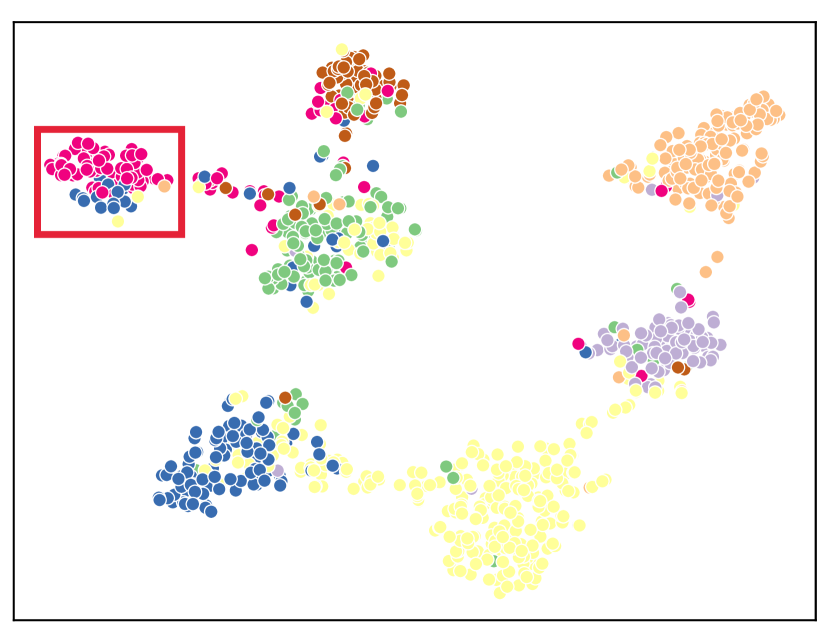
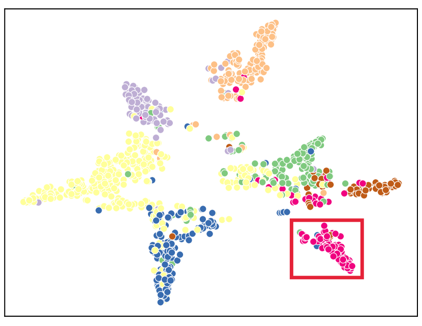
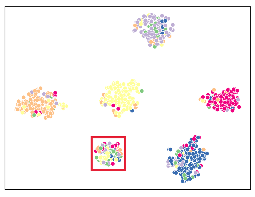
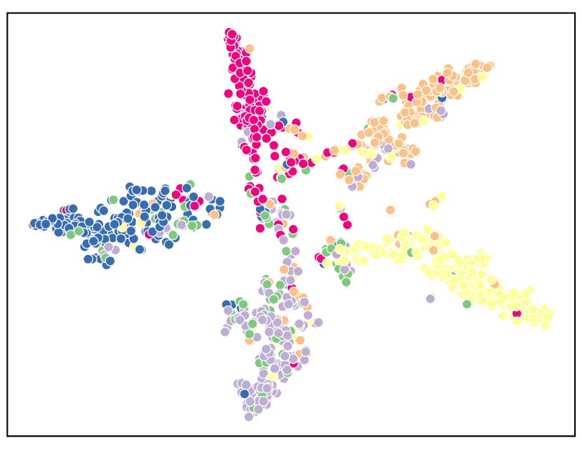
Visualization of learned representations. Figure 5 visualizes the learned representations of Self-training and DRIFT. From Fig. 5(a), we can see that Self-training mixes the representations of the red class and the blue class, as indicated in the red box. Such erroneous classification is alleviated by DRIFT (Fig. 5(b)). On Citeseer, notice that Self-training generates a meaningless cluster (Fig. 5(c)), which is a sign that Self-training overfits on the label noise.
Appendix B Classification and Named Entity Recognition Datasets
Dataset statistics for the classification and named entity recognition tasks are presented in Table 7.
| Dataset | Task | #Class | #Train | #Dev | #Test |
| AGNews | Topic | 4 | 108k | 12k | 7.6k |
| IMDB | Sentiment | 2 | 20k | 2.5k | 2.5k |
| Yelp | Sentiment | 2 | 30.4k | 3.8k | 3.8k |
| Amazon | Sentiment | 2 | 25k | 2.5k | 2.5k |
| MIT-R | Slot Filling | 9 | 6.6k | 1.0k | 1.5k |
| CoNLL-03 | NER | 4 | 14.0k | 3.2k | 3.4k |
| Webpage | NER | 4 | 385 | 99 | 135 |
| Wikigold | NER | 4 | 1.1k | 280 | 274 |
| BC5CDR | NER | 2 | 4.5k | 4.5k | 4.7k |
Appendix C Weak Supervision Sources
There are two types of semantic rules that we apply as weak supervisions:
-
•
Keyword Rule: HAS(x, L) C. If matches one of the words in the list , we label it as .
-
•
Pattern Rule: MATCH(x, R) C. If matches the regular expression , we label it as .
Two examples of semantic rules on AGNews and IMDB are given in Table 8 and Table 9.
All of the weak supervisions, i.e., linguistic rules, are from existing literature. The details are listed below:
-
•
AGNews, IMDB, Yelp: We use the rules in Ren et al. (2020).
-
•
MIT-R: We use the rules in Awasthi et al. (2020).
-
•
CoNLL-03, WebPage, Wikigold: We use the keywords in Liang et al. (2020).
-
•
BC5CDR: We use the keywords in Shang et al. (2018). Note that for simplicity, we do not use AutoPhrase to extract external keywords. Such an approach requires external corpus and extra parameter-tuning.
| Rule |
| [war, prime minister, president, commander, minister, military, militant, kill, operator] POLITICS |
| [baseball, basketball, soccer, football, boxing, swimming, world cup, nba,olympics,final, fifa] SPORTS |
| [delta, cola, toyota, costco, gucci, citibank, airlines] BUSINESS |
| [technology, engineering, science, research, cpu, windows, unix, system, computing, compute] TECHNOLOGY |
| Rule |
| [masterpiece, outstanding, perfect, great, good, nice, best, excellent, worthy, awesome, enjoy, positive, pleasant, wonderful, amazing, superb, fantastic, marvellous, fabulous] POS |
| [bad, worst, horrible, awful, terrible, crap, shit, garbage, rubbish, waste] NEG |
| [beautiful, handsome, talented] POS |
| [fast forward, n t finish] NEG |
| [well written, absorbing,attractive, innovative, instructive,interesting, touching, moving] POS |
| [to sleep, fell asleep, boring, dull, plain] NEG |
| [ than this, than the film, than the movie] NEG |
| MATCH(x, *PRE*EXP* ) POS PRE = [will , ll , would , can’t wait to ] EXP = [ next time, again, rewatch, anymore, rewind] |
| PRE = [highly , do , would , definitely , certainly , strongly , i , we ] EXP = [ recommend, nominate] |
| PRE = [high , timeless , priceless , has , great , of , real , instructive ] EXP = [ value, quality, meaning, significance] |
Appendix D Training Details
We use a validation set to tune DRIFT as well as all the baseline methods. We report the test result of the best model on the validation set. All the experimental results have passed a paired t-test with .
D.1 Baseline Settings
We implement the GraphVAT method by ourselves.
For the other baselines, we follow the official release:
(1) MixText: https://github.com/GT-SALT/MixText/;
(2) BOND: https://github.com/cliang1453/BOND;
(3) UAST: https://github.com/microsoft/UST;
(4) WeSTClass: https://github.com/yumeng5/WeSTClass;
(5) GCN: https://github.com/tkipf/pygcn;
(6) GRAND: https://github.com/THUDM/GRAND;
(7) GraphMix: https://github.com/vikasverma1077/GraphMix.
| Hyper-parameter | AGNews | IMDB | Yelp | MIT-R | CoNLL-03 | Webpage | Wikigold | BC5CDR |
| Dropout Ratio | 0.1 | |||||||
| Maximum Tokens | 128 | 256 | 512 | 64 | 128 | 128 | 128 | 128 |
| Batch Size | 32 | 16 | 16 | 64 | 32 | 32 | 32 | 32 |
| Weight Decay | ||||||||
| Learning Rate | ||||||||
| Initialization Steps | 160 | 160 | 200 | 150 | 900 | 300 | 3500 | 1500 |
| 3000 | 2500 | 2500 | 1000 | 1800 | 200 | 700 | 1000 | |
| 0.95 | 0.9 | 0.95 | 0.9 | 0.9 | 0.95 | 0.9 | 0.9 | |
| 0.5 | 0.5 | 0.5 | 0.5 | 0.5 | 0.5 | 0.5 | 0.5 | |
| Hyper-parameter | AGNews | IMDB | Amazon |
| Dropout Ratio | 0.1 | ||
| Maximum Tokens | 128 | 256 | 256 |
| Batch Size | 32 | 16 | 16 |
| Weight Decay | |||
| Learning Rate | |||
| Initialization Steps | 1200 | 1000 | 800 |
| 4000 | 3000 | 4000 | |
| 0.95 | 0.99 | 0.9 | |
| 0.6 | 0.5 | 0.5 | |
D.2 Weakly-Supervised Text Classification
Hyper-parameters are shown in Table 10.
D.3 Semi-Supervised Text Classification
We implement TextCNN with Pytorch Paszke et al. (2019). We use the pre-trained 300 dimension FastText embeddings333We use the 1 million word vectors trained on Wikipedia 2017, UMBC webbase corpus and news dataset, which is available online: https://fasttext.cc/docs/en/english-vectors.html. as the input vectors. Then, we set the filter window sizes to 2, 3, 4, 5 with 500 feature maps each. We train the model for 100 iterations as initialization, and set during self-training. We use Stochastic Gradient Descent (SGD) with momentum and we set the learning rate to . We set the dropout rate to 0.5 for the linear layers after the CNN. We tune the weight decay in .
Hyper-parameters are shown in Table 11.
D.4 Semi-Supervised Learning on Graphs
Our method serves as an efficient drop-in module to existing methods. There are only two parameters that we tune in the experiments: the exponential moving average rate and the temperature of the soft pseudo-labels. For all the three datasets, we set . For the temperature parameter, we use the following settings.
-
•
Cora: for GRAND and for GCN.
-
•
Citeseer: for GRAND and for GCN.
-
•
Pubmed: for GRAND and for GCN.
Other hyper-parameters and tricks used in training follow the corresponding works.