ARCH: Efficient Adversarial Regularized Training with Caching

Abstract

Adversarial regularization can improve model generalization in many natural language processing tasks. However, conventional approaches are computationally expensive since they need to generate a perturbation for each sample in each epoch. We propose a new adversarial regularization method ARCH (adversarial regularization with caching), where perturbations are generated and cached once every several epochs. As caching all the perturbations imposes memory usage concerns, we adopt a K-nearest neighbors-based strategy to tackle this issue. The strategy only requires caching a small amount of perturbations, without introducing additional training time. We evaluate our proposed method on a set of neural machine translation and natural language understanding tasks. We observe that ARCH significantly eases the computational burden (saves up to 70% of computational time in comparison with conventional approaches). More surprisingly, by reducing the variance of stochastic gradients, ARCH produces a notably better (in most of the tasks) or comparable model generalization. Our code is available at https://github.com/SimiaoZuo/Caching-Adv.

1 Introduction

Adversarial regularization Miyato et al. (2017) can improve model generalization in many natural language processing tasks, such as neural machine translation Cheng et al. (2019), natural language understanding Jiang et al. (2020), language modeling Wang et al. (2019b), and reading comprehension Jia and Liang (2017). Even though the method has demonstrated its power in many scenarios, its computational efficiency remains unsatisfactory.

Conventional adversarial regularization Miyato et al. (2017) methods involve a min-max optimization problem. Specifically, a perturbation is generated for each sample by solving a maximization problem, and the model parameters are subsequently updated through a minimization problem, subject to the generated perturbations. A popular algorithm Madry et al. (2018) for such optimization is to alternate between several projected gradient descent steps (PGD, for the maximization) and a gradient descent step (for the minimization).

There are two drawbacks with the alternating gradient descent/ascent method. First, the procedure requires significant computational efforts. Suppose we run PGD for $S$ steps, then we introduce extra $S$ forward passes and extra $S$ backward passes in each iteration. As such, training with adversarial regularization is significantly slower than standard training. Second, optimizing the min-max problem is hard. This is because the perturbations are model and data dependent, and thus, variance of them is large. That is, the model needs to adapt to drastically different “noisy data” (i.e., clean data with perturbations), such that the stochastic gradients vary significantly during training. Such large variance imposes optimization challenges.

We propose ARCH (Adversarial Regularization with CacHing) that alleviates the aforementioned issues by reusing perturbations. Recall that in conventional adversarial regularization methods, a different perturbation is generated for each sample in each epoch. In contrast to this, we propose to generate perturbations less frequently. For example, for a given sample, we can generate a new perturbation every 20 epochs, and the sample’s perturbation remains unchanged in other epochs. We call this method “caching”. The method has two advantages. First, it alleviates the computational burden. By reusing the perturbations, we avoid the extra forward and backward passes caused by PGD for most of the iterations. Second, caching stabilizes the stochastic gradients. Notice that in our method, the model is optimized with respect to the same noisy data for multiple times, instead of only one. In this way, variance of the stochastic gradients is reduced.

One caveat of the caching method is its memory overhead. This is because a sample’s perturbation is significantly larger than itself (the perturbation has an extra embedding dimension). We propose a K-nearest neighbors-based approach to tackle this problem. Specifically, instead of caching perturbations for all the samples, we only cache a small proportion of them. Each uncached perturbation can then be constructed using the cached ones in its neighborhood. Such a construction procedure can be executed in parallel with model training. Therefore, training time will not be prolonged because of this memory saving strategy.

We use a moving average approach to boost model generalization. Specifically, when generating a new perturbation, we integrate information from both the current model and the current perturbation. This is different from conventional approaches, where the new perturbation only depends on the current model. The moving average approach has a smoothing effect that boosts model generalization, as demonstrated both theoretically and empirically by previous works Izmailov et al. (2018); Athiwaratkun et al. (2019); Jiang et al. (2020).

Arguably, the perturbations introduced by our method may not constitute strong adversarial attacks, because of the “staleness” caused by infrequent updates. However, we highlight that the focus of this work is model generalization over clean data, instead of adversarial robustness (ability to defend attacks). As we will demonstrate in the experiments, the “weak” perturbations show notable improvement of model generalization. And somewhat surprisingly, ARCH also exhibits on par or even better robustness comparing with conventional approaches.

We conduct extensive experiments on neural machine translation (NMT) and natural language understanding (NLU) tasks. In comparison with conventional adversarial regularization approaches, ARCH can save up to 70% computational time. Moreover, in NMT tasks, our method improves about 0.5 BLUE over baseline methods on seven datasets. ARCH also achieves 0.7 average score improvement on the GLUE Wang et al. (2019a) development set over existing methods.

We summarize our contributions as follows: (1) We propose a caching method that needs drastically less computational efforts. The method can also improve model generalization by reducing variance of stochastic gradient. (2) We propose a memory saving strategy to efficiently implement the caching method. (3) Extensive experiments on neural machine translation and natural language understanding demonstrate the efficiency and effectiveness of the proposed method.

2 Background

$\diamond$ Neural machine translation has achieved superior empirical performance Bahdanau et al. (2015); Gehring et al. (2017); Vaswani et al. (2017). Recently, the Transformer Vaswani et al. (2017) architecture dominates the field. This sequence-to-sequence model employs an encoder-decoder structure, and also integrates the attention mechanism. During the encoding phase, a Transformer model first computes an embedding for each sentence, after which the embeddings are fed into several layers of encoding blocks. Each of these blocks contain a self-attention mechanism and a feed-forward neural network (FFN). Subsequently, after encoding, the hidden representations are fed into the decoding blocks, each constituted of a self-attention, a encoder-decoder attention, and a FFN.

$\diamond$ Fine-tuning pre-trained language models Peters et al. (2018); Devlin et al. (2019); Radford et al. (2019); Liu et al. (2019b); He et al. (2020) is a state-of-the-art method for natural language understanding tasks such as the GLUE Wang et al. (2019a) benchmark. Adversarial regularization is also incorporated into the fine-tuning approach. For example, Liu et al. (2020a) combines adversarial pre-training and fine-tuning, Zhu et al. (2020); Jiang et al. (2020) adopt trust region-based methods, and Aghajanyan et al. (2020) aims for a more efficient computation.

$\diamond$ Adversarial training was originally proposed for computer vision tasks Szegedy et al. (2014); Goodfellow et al. (2015); Madry et al. (2018), where the goal is to train robust classifiers. Such methods synthesize adversarial samples, such that the classifier is trained to be robust against them. This strategy is also effective for tasks beyond computer vision, such as in reinforcement learning Shen et al. (2020). Various algorithms are proposed to craft the adversarial samples, e.g., learning-to-learn Jiang et al. (2021) and Stackelberg adversarial training Zuo et al. (2021). Moreover, adversarial training is also well-studied theoretically Li et al. (2019). In natural language processing, the goal is no longer adversarial robustness, but instead we use adversarial regularization to boost model generalization. Note that adversarial training and adversarial regularization are different concepts. The former focuses on defending against adversarial attacks, and the latter focuses on encouraging smooth model predictions Miyato et al. (2017). These two goals are usually treated as mutually exclusive Raghunathan et al. (2020); Min et al. (2020).

3 Method

Generating perturbations for natural language inputs faces the difficulty of discreteness, i.e., words are defined in a discrete space. A common approach to tackle this is to work on the continuous embedding space Miyato et al. (2017); Sato et al. (2019). Denote $f(x,\theta)$ a neural network parameterized by $\theta$, where $x$ is the input embedding. Further denote $y$ the ground-truth corresponding to $x$. For example, in classification tasks, $x$ is the sentence embedding, and $y$ is its label. In sequence-to-sequence learning, $x$ is the source sentence embedding, and $y$ is the target sentence. In both of these cases, the model is trained by minimizing the empirical risk over the training data, i.e.,

$$\min_{\theta}\mathcal{L}(\theta)=\frac{1}{n}\sum_{i=1}^{n}\ell(f(x_{i},\theta),y_{i}).$$

Here $\{(x_{i},y_{i})\}_{i=1}^{n}$ is the dataset, and $\ell$ is a task-specific loss, e.g., cross-entropy loss for classification and mean-squared error for regression.

3.1 Adversarial Regularization

Adversarial regularization Miyato et al. (2017) is a technique that encourages smoothness of the model outputs around each input data point. Concretely, we define an adversarial regularizer for non-regression tasks as

$$\ell_{v}(x,\delta,\theta)=\mathrm{KL}\big{(}f(x,\theta)~{}||~{}f(x+\delta,\theta)\big{)},$$

$$\text{where }\mathrm{KL}(P~{}||~{}Q)=\sum_{k}p_{k}\log\frac{p_{k}}{q_{k}}.$$

Here $f(\cdot,\theta)$ is the prediction confidence, i.e., $\sum_{i}[f(\cdot,\theta)]_{i}=1$, $\delta$ is the perturbation of sample $x$, and $\mathrm{KL}(\cdot||\cdot)$ is the Kullback–Leibler (KL) divergence. In regression tasks, the model output $f(\cdot,\theta)$ is a scalar, and the adversarial regularizer is

$$\ell_{v}\left(x,\delta,\theta)=(f(x,\theta)-f(x+\delta,\theta)\right)^{2}.$$

We consider the worst-case perturbation to encourage the model to make smooth predictions. Specifically, at epoch $t$, we solve

$$\min_{\theta^{t}}\mathcal{L}(\theta^{t})+\frac{\lambda}{n}\sum_{i=1}^{n}\max_{\left\lVert\delta_{i}^{t}\right\rVert\leq\epsilon}\ell_{v}(x_{i},\delta_{i}^{t},\theta^{t}).$$ (1)

Here $\lambda$ is the weight of the regularizer, $\epsilon$ is a pre-defined perturbation strength, and $\left\lVert\cdot\right\rVert$ is either the $\ell_{2}$ norm or the $\ell_{\infty}$ norm. Notice that the perturbation $\delta_{i}^{t}$ of sample $x_{i}$ is different in each epoch.

The min-max optimization problem in Eq. 1 is notoriously difficult to solve. Previous works Miyato et al. (2017); Sato et al. (2019); Jiang et al. (2020); Zhu et al. (2020) employ variations of alternating gradient descent/ascent. That is, we first solve the maximization problem using several iterations of projected gradient ascent, and then we run a gradient descent step on the loss function of the minimization problem, subject to the generated perturbations. The above procedures are run iteratively.

On major drawback of the alternating gradient descent/ascent approach is that the stochastic gradients are unstable. Specifically, norms of the gradients vary significantly during training (Fig. 3). This is because perturbations are generated based on the current model parameters, i.e., by maximizing $\ell_{v}(x_{i},\delta_{i}^{t},\theta^{t})$, where $\theta^{t}$ changes in each epoch. Therefore, the perturbations exhibit large variance. This causes instability of the stochastic gradients, because the model needs to adapt to drastically different adversarial directions (i.e., $\delta_{i}^{t}$).

3.2 Adversarial Regularization with Caching

To alleviate the gradient instability problem, we propose to reuse the perturbations. Specifically, instead of optimizing with respect to different perturbations $\{\delta_{i}^{t}\}_{i=1}^{n}$ in each epoch, we optimize with respect to the same ones for several epochs.

Concretely, the training objective is now

$$\min_{\theta^{t}}\mathcal{L}(\theta^{t})+\frac{\lambda}{n}\sum_{i=1}^{n}\ell_{v}(x_{i},\delta_{i}^{t},\theta^{t}),$$ (2)

$$\delta_{i}^{t}=\begin{cases}\delta_{i}^{t-1},&t\%T_{c}\neq 0,\\ \alpha\delta_{i}^{t-1}+(1-\alpha)\Delta_{i}^{t},&t\%T_{c}=0.\end{cases}$$

$$\quad\text{where }\Delta_{i}^{t}=\max_{\left\lVert\delta_{i}^{t}\right\rVert\leq\epsilon}\ell_{v}(x_{i},\delta_{i}^{t},\theta^{t}).$$

Here, $\%$ is the mod operator, and $T_{c}$ is a pre-defined gap between re-computing the perturbations. Notice that we use an exponential moving average (EMA) approach with parameter $\alpha$ when updating the perturbations. The EMA strategy integrates past information into the current epoch, and induces a smoothing effect that boosts model generalization. This strategy has demonstrated its effectiveness in many previous works Izmailov et al. (2018); Athiwaratkun et al. (2019); Jiang et al. (2020).

In comparison with Eq. 1, the formulation in Eq. 2 indicates that the perturbations are generated $\lfloor T/T_{c}\rfloor$ times instead of $T$ times when we train for $T$ epochs. As such, the model is optimized with respect to $\{\delta_{i}\}_{i=1}^{n}$ for $T_{c}$ times, instead of only one time. In this way, the model can better adapt to the perturbed data, and thus, variance of the gradient norms is reduced. Intuitively, this is because optimization is more stable when the model is trained on the same data for multiple epochs, in comparison with trained on different noisy data in each epoch. The algorithm to implement the caching strategy is summarized in Algorithm 1.

In conventional adversarial regularization (e.g., SMART), we find the perturbations by optimization algorithms such as projected gradient decent at every iteration. Recently, R3F Aghajanyan et al. (2020) propose to use random perturbations instead, i.e., they directly draw $\delta$ from a normal distribution, and generalization of R3F can match SMART in some cases. However, because the random noise (as opposed to optimized perturbations) is not data-dependent, generalization of R3F is subpar in some scenarios, e.g., machine translation (see our experiments). Our approach enjoys the advantages of both of these two methods. Specifically, ARCH is efficient since it remove the maximization problem most of the time. Moreover, perturbations generated by our method are informative, unlike R3F. Empirically, our proposed method is just as efficient as R3F, and somewhat surprisingly, we find that generalization of ARCH can not only match, but even surpass conventional approaches in most of the tasks (see our experiments).

Input: $T$: number of training epochs; $T_{c}$: number of epochs between caching; $\alpha$: moving average parameter.

Initialize: Cache $\mathcal{C}=\text{dict}\{\}$;

for $t=0,\cdots T-1$ do

       for each batch $\mathcal{B}$ do

             // Find perturbations

             if $t\%T_{c}==0$ then

                   Find $\delta_{i}^{t}$ for each $x_{i}\in\mathcal{B}$ using projected gradient ascent;

                   $\mathcal{C}[x_{i}]\leftarrow\alpha\mathcal{C}[x_{i}]+(1-\alpha)\delta_{i}^{t}$ for each $x_{i}\in\mathcal{B}$;

                  

             else

                   $\delta_{i}^{t}=\mathcal{C}[x_{i}]$ for each $x_{i}\in\mathcal{B}$;

                  

             end if

            // Update model

             One-step gradient descent on Eq. 2;

            

       end for

      

end for

Output: Trained model.

Algorithm 1 Adversarial Regularization with Caching.

3.3 Memory Saving with KNN

One caveat of Algorithm 1 is the increased memory usage. For example, there are about 4.5 million sentence pairs in the WMT’16 En-De dataset, so that simply caching the adversarial samples takes about 100GB of memory. We propose a memory saving strategy based on K-nearest neighbors (KNN) to address this issue.

Input: $W$: word embedding matrix; $n$: total number of training samples; $p$: proportion of cached samples; $K$: size of each neighbor.

// Before training

Compute $\{v_{i}\}_{i=1}^{n}$ using $W$ and Eq. 4;

Sample a cache set $\mathcal{X}\subset\{1\cdots n\}$ such that $|\mathcal{X}|=\lfloor np\rfloor$;

for $i\in\{1\cdots n\}\setminus\mathcal{X}$ do

       Find $\mathcal{K}_{i}\subset\mathcal{X}$ for $x_{i}$ based on cosine similarity among $\{v_{i}\}_{i=1}^{n}$;

      

end for

// In epoch $t$ where $t\%T_{c}\neq 0$

for $i=1,\cdots n$ do

       if $i\in\mathcal{X}$ then

             Retrieve $\delta^{t}_{i}$ from cache;

            

       else

             Compute $\delta_{i}^{t}$ using $\mathcal{K}_{i}$ and Eq. 3;

            

       end if

      

end for

Algorithm 2 Memory Saving.

The idea is to only cache perturbations of some samples, and perturbations of the other samples are constructed using the cached ones on the fly. Specifically, whenever $t\%T_{c}=0$, i.e., we need to re-compute and re-cache the perturbations, we only cache $\delta_{i}^{t}$ such that $i\in\mathcal{X}$. Here, $\mathcal{X}\subset\{1\cdots n\}$ is a pre-defined cache set and $|\mathcal{X}|\ll n$. This strategy significantly reduces memory overhead. Consequently, in each epoch $t$ where $t\%T_{c}\neq 0$, perturbations $\delta_{i}^{t}$ such that $i\in\mathcal{X}$ are directly retrieved from the cache. And perturbations $\delta_{i}^{t}$ such that $i\in\{1\cdots n\}\setminus\mathcal{X}$ are defined as the following:

$$\delta^{t}_{i,\ell}=\frac{1}{|\mathcal{K}_{i}|}\sum_{j\in\mathcal{K}_{i}}\frac{1}{\ell_{j}}\sum_{\ell^{\prime}=1}^{\ell_{j}}\delta^{t-1}_{j,\ell^{\prime}},\ \ell=1,\cdots,\ell_{i}.$$ (3)

Here, $\ell_{i}$ be the length of sentence $x_{i}$, $\delta^{t}_{i,\ell}\in\mathbb{R}^{d}$ is the perturbation for the $\ell$-th word in sentence $x_{i}$, and $\mathcal{K}_{i}$ is the nearest neighbor set for $x_{i}$ (which we present later). We remark that constructing the perturbations does not impose extra training time, because we can perform such computation in parallel with training.

We remark that each word has an identical perturbation in Eq. 3, i.e., $\delta^{t}_{i}\in\mathbb{R}^{|\ell_{i}|\times d}$ has identical rows. We choose this design because a perturbation in the neighbor of $\delta_{i}^{t}$ may have a different dimension, i.e., $\delta^{t}_{j}\in\mathbb{R}^{|\ell_{j}|\times d}$ is in the neighbor of $\delta^{t}_{i}$ and it is possible that $|\ell_{i}|\neq|\ell_{j}|$. To resolve this issue, we compute the word-level mean of all the perturbations in the neighbor of $\delta_{i}^{t}$ and assign it to each row of $\delta^{t}_{i}$.

The remaining is to find $K$ nearest neighbors in $\mathcal{X}$ for each sentence $x_{i}$ such that $i\in\{1\cdots n\}\setminus\mathcal{X}$. Suppose we have a word embedding matrix $W\in\mathbb{R}^{d\times|\mathcal{V}|}$, where $|\mathcal{V}|$ is the vocabulary size and $d$ is the embedding dimension. Note that $W$ can be obtained from pre-trained models such BERT Devlin et al. (2019). For each sentence $x_{i}$, we compute its sentence representation $v_{i}\in\mathbb{R}^{d}$ as

$$v_{i}=\frac{1}{\ell_{i}}\sum_{\ell=1}^{\ell_{i}}Wx_{i,\ell}.$$ (4)

Here, $x_{i,\ell}\in\mathbb{R}^{|\mathcal{V}|}$ is the one-hot vector of the $\ell$-th word in sentence $x_{i}$. Then, we can find $K$ nearest neighbors $\mathcal{K}_{i}$ for sample $x_{i}$ using the KNN algorithm, where the distance between two samples is defined as their cosine similarity. Notice that finding $\{\mathcal{K}_{i}\}_{i=1}^{n}$ is a pre-processing step, i.e., we can find the neighbors before training the model.

The memory saving algorithm is summarized in Algorithm 2, and an extended version that combines caching and memory saving is presented in Algorithm 3 in the appendix.

3.4 Computational Efficiency

Computational costs of various methods are summarized in Table 1. In conventional adversarial regularization algorithms, such as FreeLB Zhu et al. (2020) and SMART Jiang et al. (2020), suppose we solve the inner maximization problem for $S$ steps, then we impose extra $S$ forward passes and $S$ backward passes in each iteration. In contrast, R3F Aghajanyan et al. (2020) removes the maximization problem, and directly samples perturbations from a normal distribution. Thus, R3F only introduce one extra forward pass to compute the regularization term. Using Algorithm 1, our method shares similar efficiency as R3F. Specifically, suppose we cache the perturbations every $T_{c}$ epochs, then the average number of forward passes and backward passes per iteration is $2+(S-1)/T_{c}$ and $1+S/T_{c}$, respectively. In practice, $S/T_{c}$ is usually small, such that the computational cost between ARCH and R3F is close.

Wall time comparison is illustrated in Fig. 1. Notice that in the left subfigure, both our method and R3F save about 70% computation time in comparison with FreeLB and SMART. In the right subfigure, the time saving is about 50%. The absolute time saving is more significant on large models and large datasets. For example, when training a Transformer-big model on the WMT’16 En-De dataset, our method costs about 176 GPU hours, while SMART uses 576 GPU hours.

	Forward	Backward
Standard	$1$	$1$
FreeLB	$1+S$	$1+S$
SMART	$1+S$	$1+S$
R3F	$2$	$1$
ARCH	$2+(S-1)/T_{c}$	$1+S/T_{c}$

Table 1: Computational cost of various methods. Here S is the number of gradient ascent (PGD) steps, and $T_{c}$ is the number of epochs between caching. Forward is the number of forward passes, and Backward is the number of backward passes.

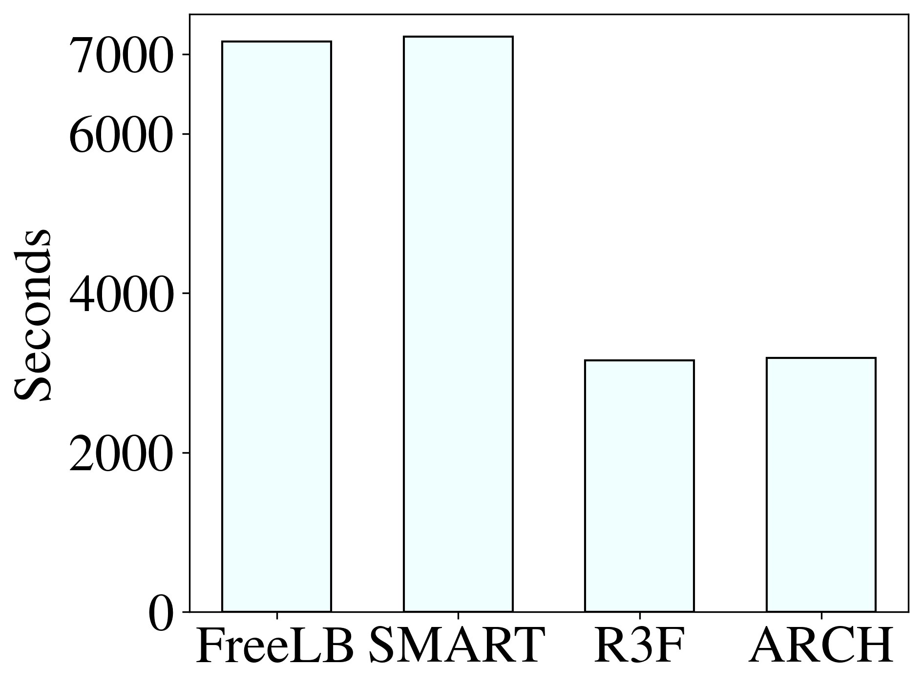
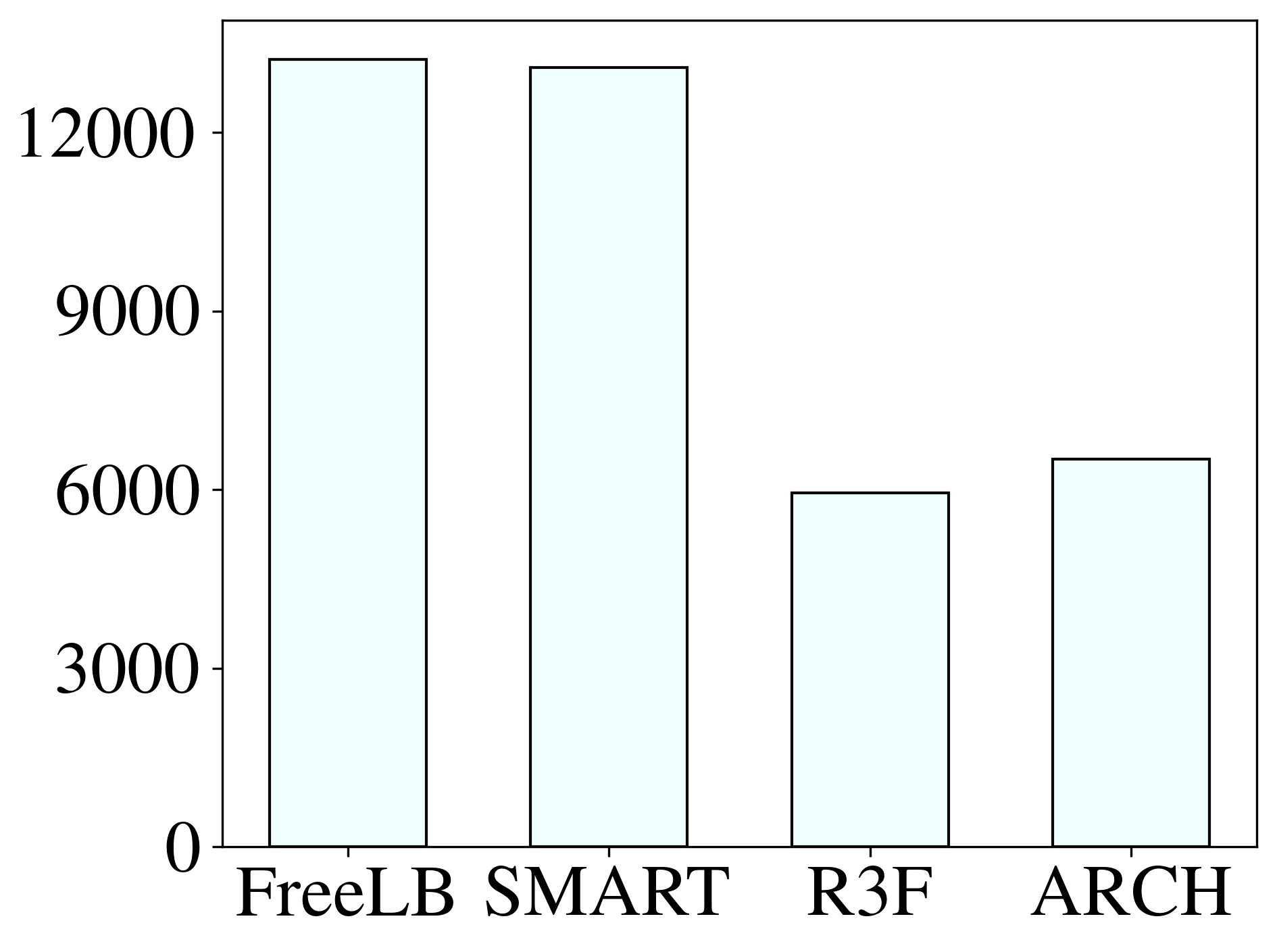
Figure 1: Wall time of different methods. Left: training a Transformer-base model for 150 epochs on IWSLT’14 De-En; Right: fine-tuning BERT_BASE for 10 epochs on SST-2.

Models	En-Vi	Vi-En	En-De	De-En	En-Fr	Fr-En
Transformer Vaswani et al. (2017)	30.3	28.7	28.3	34.7	39.3	38.2
R3F Aghajanyan et al. (2020)	31.6	30.0	29.0	35.4	39.5	38.7
FreeLB Zhu et al. (2020)	31.6	29.6	28.6	35.3	39.4	38.7
SMART Jiang et al. (2020)	31.5	30.1	29.2	35.5	39.8	38.9
ARCH	32.0	30.4	29.4	36.1	40.3	39.3

Table 2: BLEU score on three low-resource datasets. All the baseline results are from our re-implementation. We report the mean over three runs using different random seeds. ARCH saves about 70% computational time comparing with SMART.

Models	BLEU	sacreBLEU
Transformer	29.1	28.4
R3F	29.4	29.0
FreeLB	29.3	29.0
SMART	29.8	29.1
ARCH	29.8	29.4

Table 3: BLEU and sacreBLEU score on the WMT’16 En-De dataset. All the baseline results are from our re-implementation.

Data	Source	Train	Valid	Test
En-Vi	IWSLT’15	133k	768	1268
En-De	IWSLT’14	161k	7.2k	6.7k
En-Fr	IWSLT’16	224k	1080	1133
En-De	WMT’16	4.5m	3.0k	3.0k

Table 4: Dataset source and statistics. Here “k” stands for thousand, and “m” stands for million.

4 Experiments

In all the experiments, we use PyTorch Paszke et al. (2019) as the backend. All the experiments are conducted on NVIDIA V100 GPUs.

4.1 Baselines

We adopt several baselines in the experiments.

$\diamond$ Transformer Vaswani et al. (2017) achieves superior performance in neural machine translation.

$\diamond$ BERT Devlin et al. (2019) exhibits outstanding performance when fine-tuned on natural language understanding tasks.

$\diamond$ FreeAT Shafahi et al. (2019) enables “free” adversarial training by recycling the gradient information generated when updating the model.

$\diamond$ FreeLB Zhu et al. (2020) treats the intermediate perturbations during the projected gradient ascent steps as virtual batches. As such, the method achieves “free” large batch adversarial training.

$\diamond$ SMART Jiang et al. (2020) achieves state-of-the-art performance in natural language understanding. The method utilizes smoothness-inducing regularization and Bregman proximal point optimization.

$\diamond$ R3F Aghajanyan et al. (2020) replaces the maximization problem in conventional adversarial regularization with random noise.

	RTE	MRPC	CoLA	SST-2	STS-B	QNLI	QQP	MNLI-m/mm	Average
	Acc	Acc/F1	Mcc	Acc	P/S Corr	Acc	Acc/F1	Acc	Score
BERTBASE	63.5	84.1/89.0	54.7	92.9	89.2/88.8	91.1	90.9/88.3	84.5/84.4	81.5
FreeAT	68.0	85.0/89.2	57.5	93.2	89.5/89.0	91.3	91.2/88.5	84.9/85.0	82.6
FreeLB	70.0	86.0/90.0	58.9	93.4	89.7/89.2	91.5	91.4/88.4	85.4/85.5	83.3
R3F	70.4	87.0/91.0	59.1	93.4	90.1/89.8	92.0	91.7/88.8	85.2/85.4	83.7
SMART	71.2	87.7/91.3	59.1	93.0	90.0/89.4	91.7	91.5/88.5	85.6/86.0	83.8
ARCH	72.2	88.0/91.6	61.1	93.6	90.6/90.2	92.2	91.9/89.1	85.6/86.0	84.5

Table 5: Evaluation results on the GLUE development set. We use the BERT_BASE architecture for all the methods. The best results on each dataset are shown in bold. Results of BERT_BASE Devlin et al. (2019), FreeAT Shafahi et al. (2019), FreeLB Zhu et al. (2020), and R3F Aghajanyan et al. (2020) are based on our re-implementation. SMART results are from Jiang et al. (2020).

4.2 Machine Translation

Datasets. We use three low-resource datasets: English-German from IWSLT’14, English-Vietnamese from IWSLT’15, and English-French from IWSLT’16. We also use a rich-resource dataset: English-German from WMT’16. Dataset statistics are summarized in Table 4.

Implementation. In NMT tasks, we have the source-side and the target-side inputs. We add perturbations to both of their embeddings Sato et al. (2019). This has demonstrated to be more effective than adding perturbations to a single side. We use Fairseq Ott et al. (2019) to implement our algorithms. For En-Vi and En-Fr experiments, we use the Transformer-base architecture Vaswani et al. (2017). For En-De (IWSLT’14) experiments, we modify the Transformer-base architecture by decreasing the hidden dimension size from 2048 to 1024, and decreasing the number of heads from 8 to 4 (while dimension of each head doubles). For En-De (WMT’16) experiments, we use the Transformer-big Vaswani et al. (2017) architecture. The training details are presented in Appendix B.1.

Results. Experimental results on the low-resource datasets are summarized in Table 2. We can see that ARCH outperforms all the baselines in all the experiments. We remark that our method saves about 70% computational time in comparison with SMART and FreeLB, and has the save level of efficiency comparing with R3F (Fig. 1). Even though R3F is efficient by eliminating the maximization problem, we can see that is does not generalize as well as SMART, i.e., R3F has worse BLEU score than SMART in 5/6 of the experiments.

Experimental results on the WMT’16 En-De dataset are summarized in Table 3. We report both the BLEU score and the sacreBLEU Post (2018) score. The former is standard for machine translation tasks, and the latter is a detokenzied version of BLEU. The absolute computational time saving is more significant for larger datasets (e.g., WMT) and larger models (e.g., Transformer-big). In the experiments, ARCH uses about 176 GPU hours to train, while it costs SMART about 576 hours. Performance of ARCH is better or on par with all the baselines. Notice that like in Table 2, performance of R3F is worse than SMART.

4.3 Natural Language Understanding

Datasets. We conduct experiments on the General Language Understanding Evaluation (GLUE) benchmark Wang et al. (2019a), which is a collection of nine natural language inference tasks. The benchmark includes question answering Rajpurkar et al. (2016), linguistic acceptability (CoLA, Warstadt et al. 2019), sentiment analysis (SST, Socher et al. 2013), text similarity (STS-B, Cer et al. 2017), paraphrase detection (MRPC, Dolan and Brockett 2005), and natural language inference (RTE & MNLI, Dagan et al. 2006; Bar-Haim et al. 2006; Giampiccolo et al. 2007; Bentivogli et al. 2009; Williams et al. 2018) tasks. Statistics of the datasets are summarized in Table 8 (Appendix B.2).

Implementation. We implement our algorithm using the MT-DNN Liu et al. (2019a, 2020b) and the Transformers Wolf et al. (2020) code-base. The training details are presented in Appendix B.2.

Results. Table 5 summarizes experimental results on the GLUE development set. We can see that ARCH is on par or outperforms all the baselines in all the tasks. Notice that generalization of R3F is comparable with SMART. Our proposed method shares the advantages of both efficiency (i.e., R3F) and informative perturbations (i.e., SMART), and thus, ARCH behaves better than both of these methods. We highlight that our method is 50%-70% faster than SMART and FreeLB.

4.4 Parameter Study

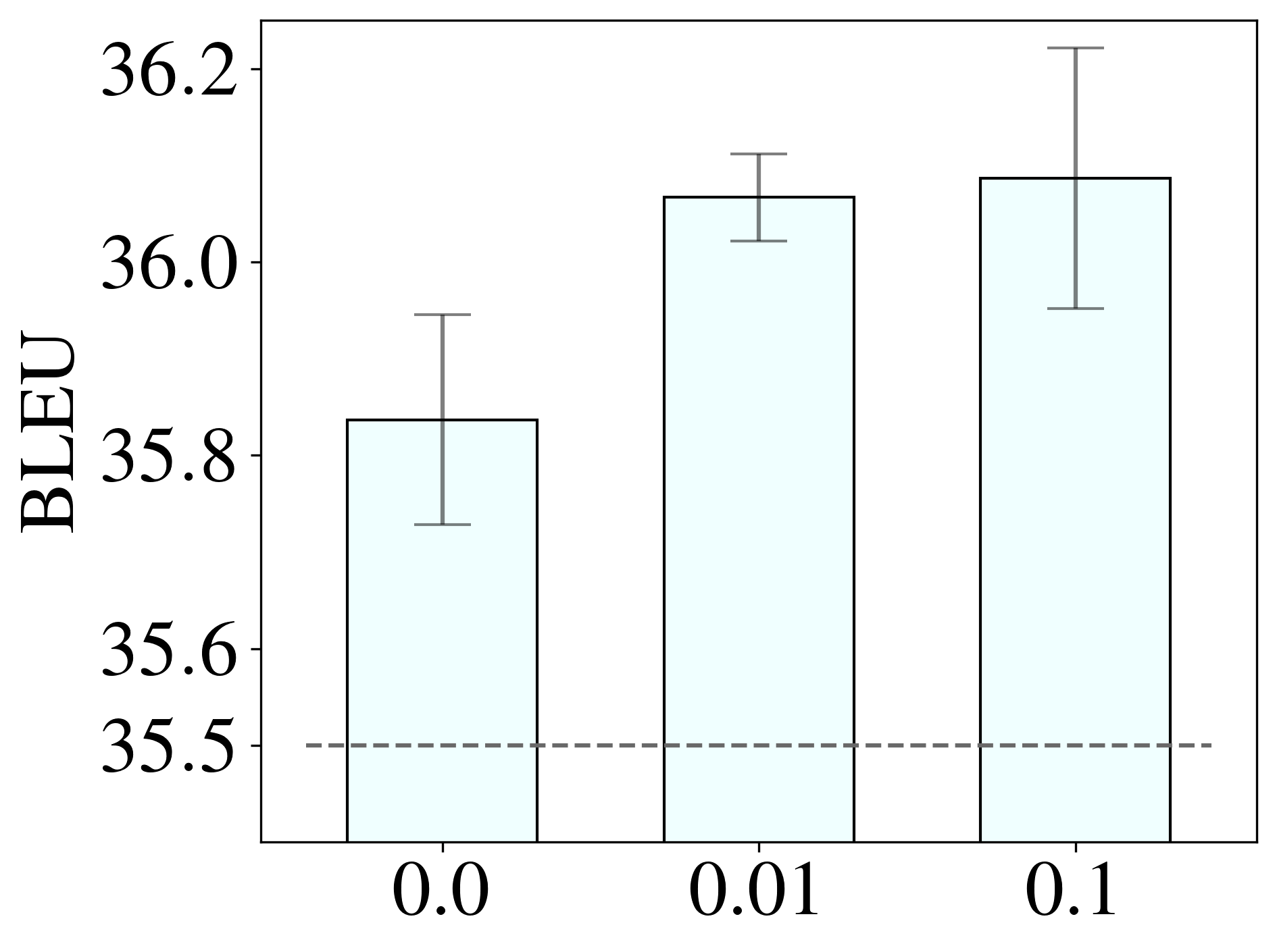
(a) Moving average.

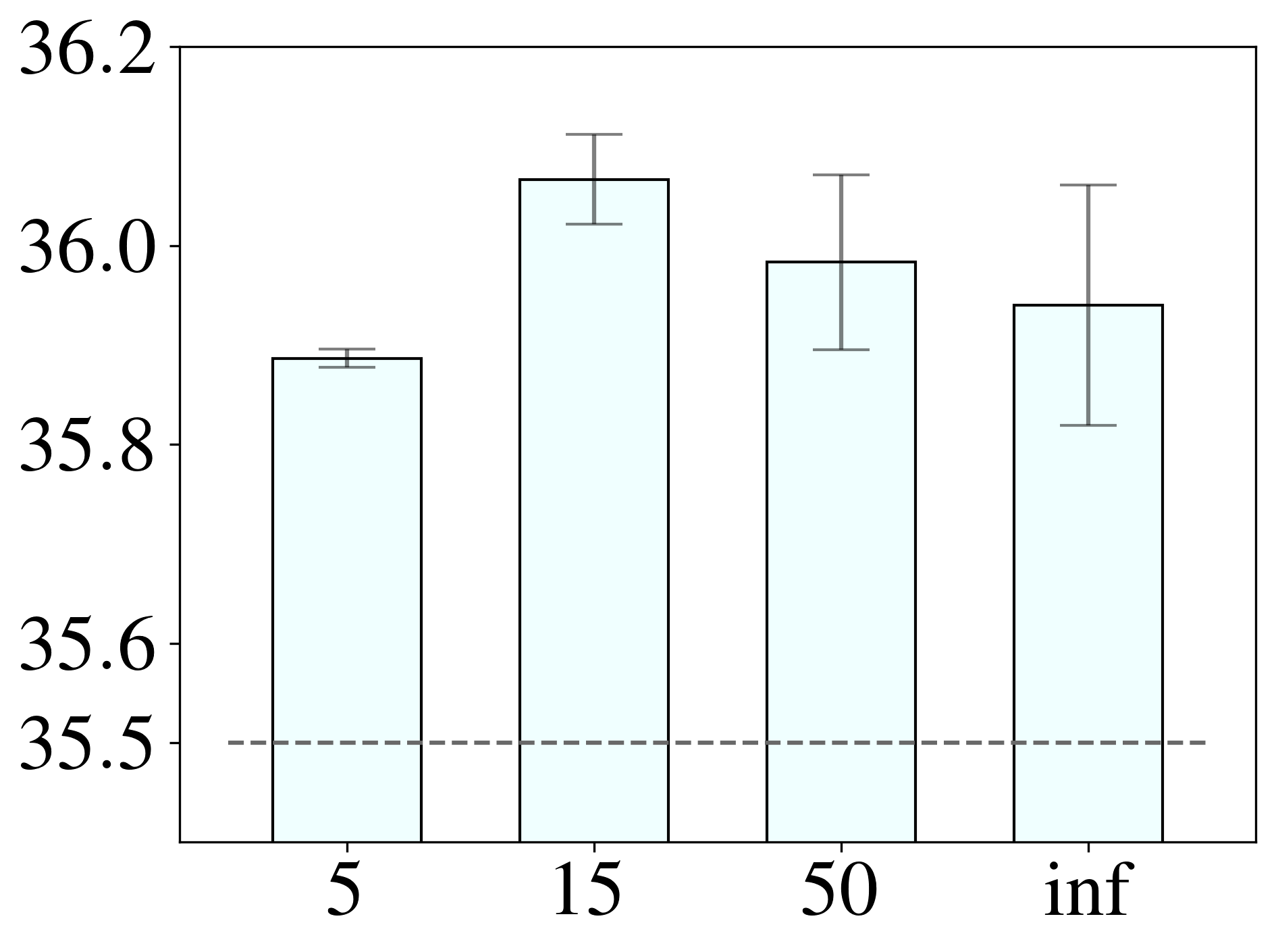
(b) Epochs between caching.

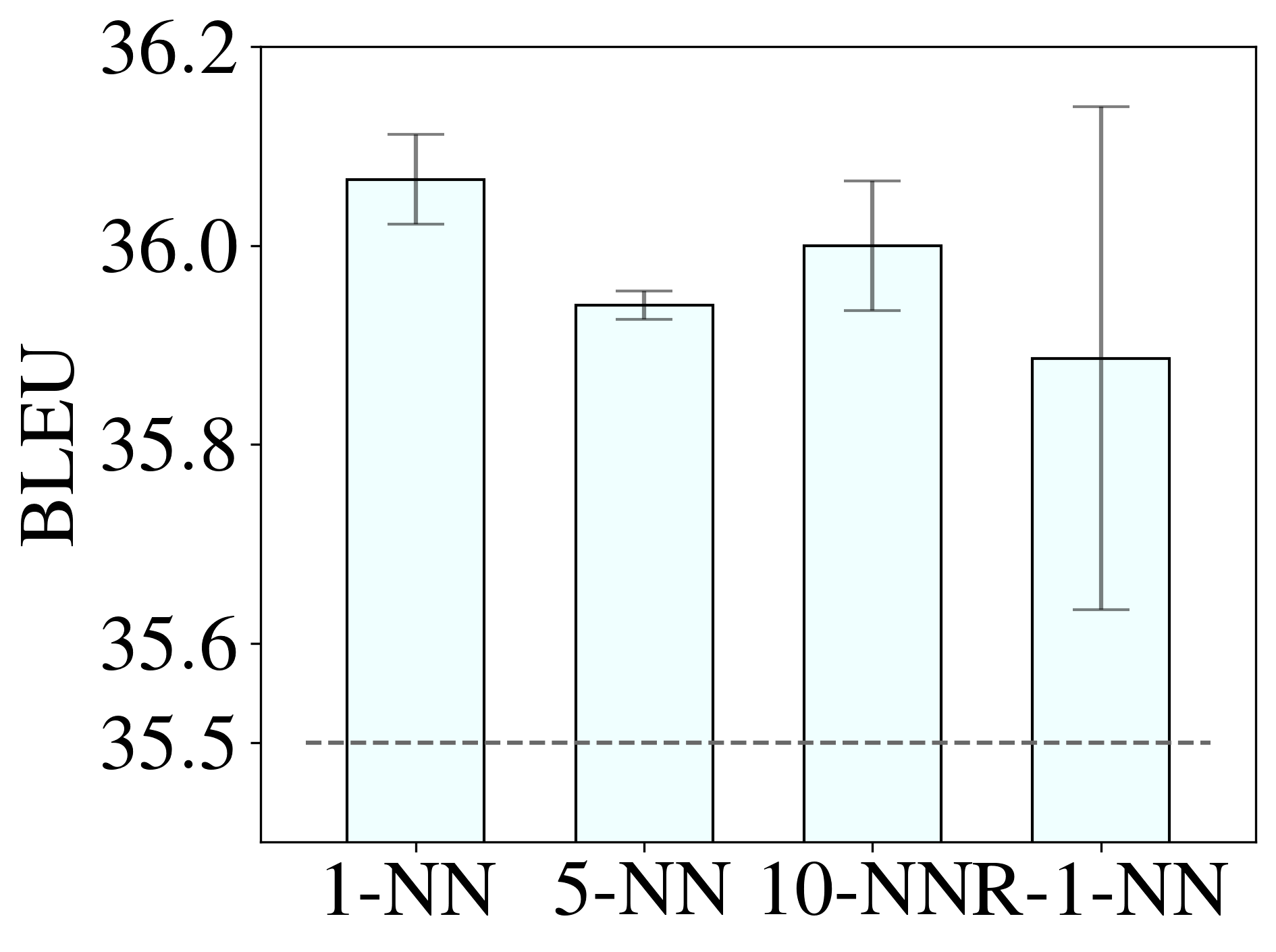
(c) Number of neighbors.

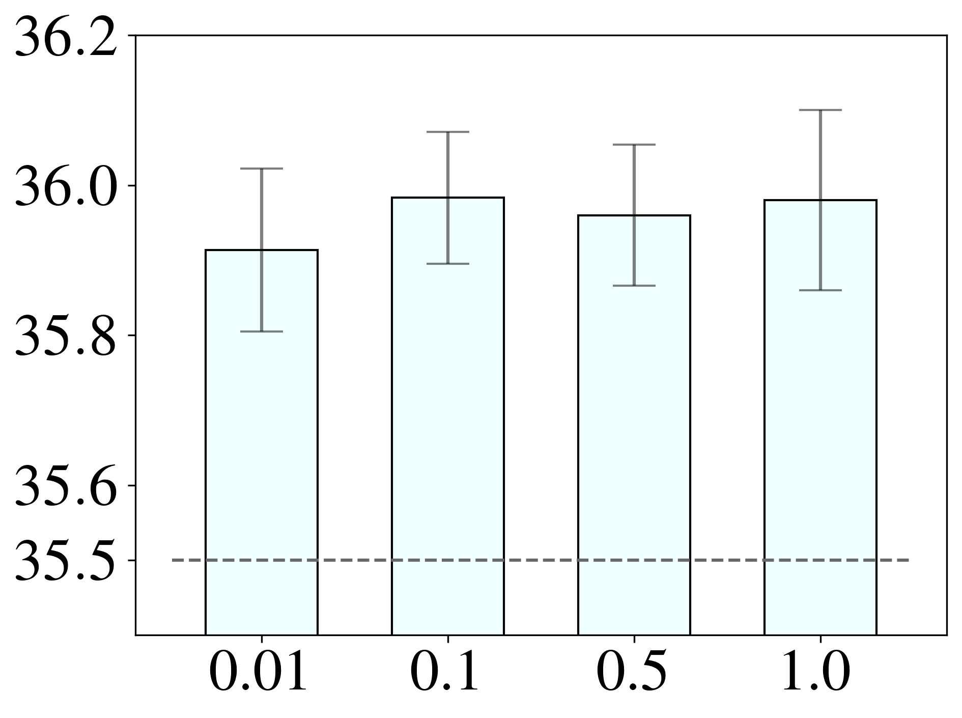
(d) Proportion of caching.

Figure 2: Parameter study on the IWSLT’14 De-En dataset. Each error bar is based on three runs using different random seeds. Each dashed line signifies the SMART baseline. In (b), inf means we only cache once during training. In (c), R-1-NN means we use 1-NN, but the neighbor is randomly selected.

$\diamond$ Moving average helps. As indicated in Fig. 2(a), without the exponential moving average, model performance drops about 0.3 BLEU. Also, the model is robust to the moving average parameter, as increasing it from 0.01 to 0.1 does not change model performance.

$\diamond$ Number of epochs between caching is important. If we cache the perturbations too frequently (i.e., 5 in Fig. 2(b)), the model cannot adapt to the perturbations well; and if we cache the perturbations too infrequently (i.e., inf in Fig. 2(b)), staleness of the perturbations hinders model generalization.

$\diamond$ Robustness to the number of neighbors. In Fig. 2(c), notice that ARCH is robust to the number of neighbors. We also examine a variant of the KNN memory-saving strategy (R-1-NN): namely in Algorithm 1, the nearest neighbors set $\mathcal{K}_{i}$ for sample $x_{i}$ is randomly constructed instead of based on word embeddings. We can see that model performance drops, and the method also exhibits drastically larger variance.

$\diamond$ Robustness to the number of cached samples. From Fig. 2(d), notice that the model generalizes well even caching only 1% of the perturbations (i.e., only 1400 samples for the IWSLT’14 De-En dataset). Moreover, the KNN memory-saving strategy does not hinder model performance, i.e., the BLEU score is consistent when caching all the samples and caching only 10% of the samples.

We highlight that in practice ARCH does not need much tuning, because the method is robust to the introduced hyper-parameters.

4.5 Analysis

$\diamond$ Caching reduces gradient norm variance. As demonstrated in Fig. 3, variance of the gradient norms reduces significantly comparing with SMART and R3F. This meets our expectation that by reusing perturbations, the model can adapt to the noisy data (i.e., clean data with perturbations) better. Notice that R3F has even larger gradient norm variance than SMART, which is because R3F uses random noise instead of data-dependent ones.

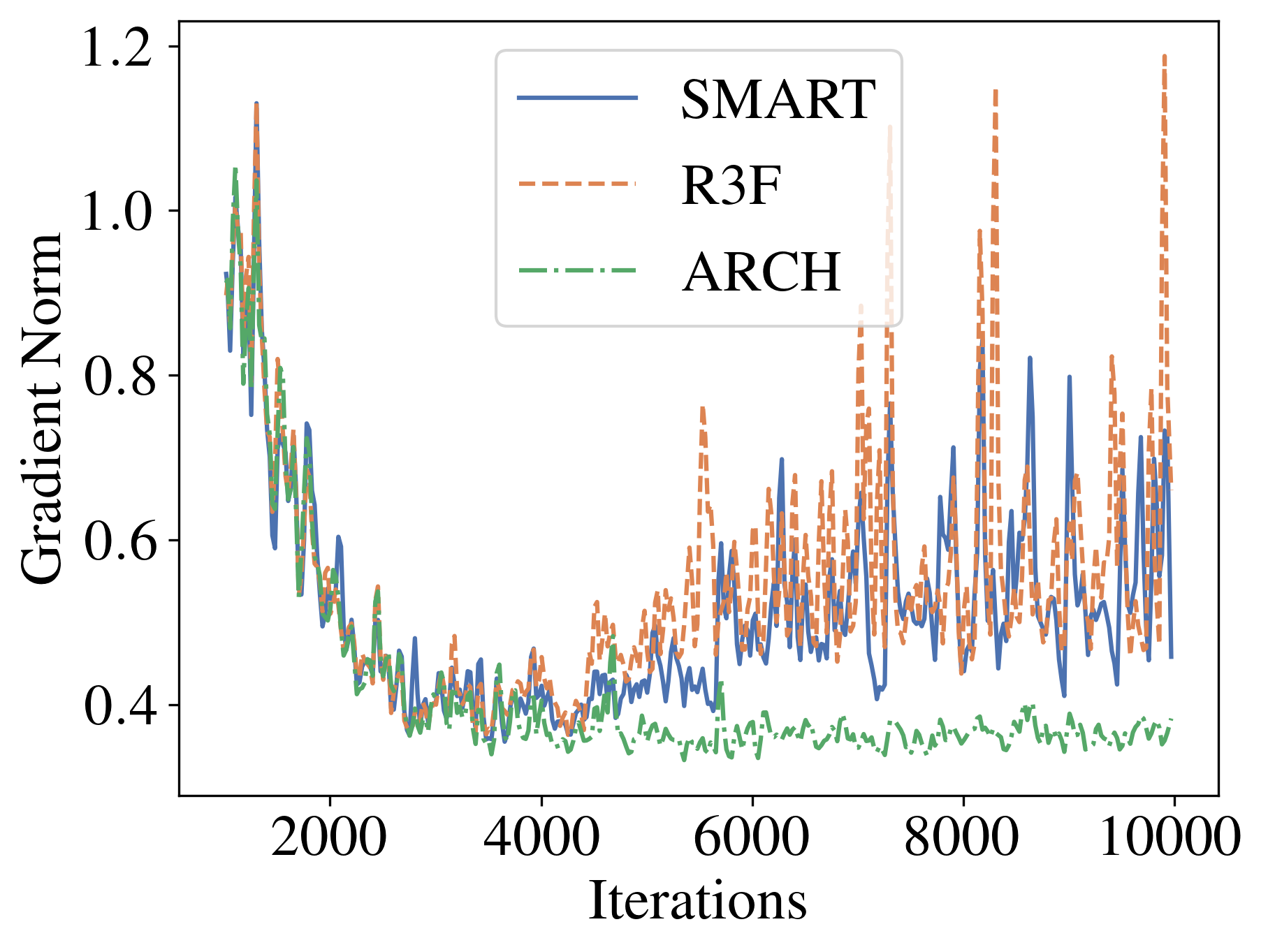
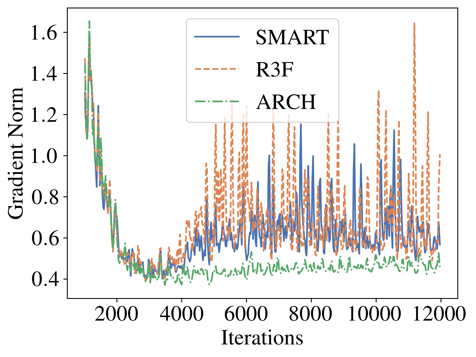
Figure 3: Norm of stochastic gradients during training. Top: IWSLT’14 De-En; Bottom: IWSLT’15 En-Vi.

$\diamond$ Adversarial robustness. We remark that the focus of ARCH is model generalization. Nevertheless, we investigate model robustness on the Adversarial-NLI (ANLI, Nie et al. 2020) dataset. The dataset contains 163k data, which are collected via a human-and-model-in-the-loop approach. Surprisingly, from Table 6, we can see that R3F and ARCH achieve on par robustness with SMART. This indicates that reusing perturbations, or even constructing random perturbations can increase robustness (than BERT) to the same level as computing optimized perturbations (i.e., SMART).

	Dev
	R1	R2	R3	All
BERTBASE	53.3	43.0	44.7	46.8
R3F	53.9	43.4	46.3	47.8
SMART	54.1	44.4	45.3	47.8
ARCH	54.0	46.1	46.0	48.5
	Test
	R1	R2	R3	All
BERTBASE	54.1	44.9	46.6	48.4
R3F	54.3	46.2	46.5	48.8
SMART	54.3	46.4	46.5	48.9
ARCH	53.8	46.6	47.4	49.2

Table 6: Experimental results on the ANLI dataset. Model references: BERT_BASE Devlin et al. (2019), R3F Aghajanyan et al. (2020), SMART Jiang et al. (2020).

$\diamond$ Probing experiments. We first fine-tune a BERT_BASE model on the SST-2 dataset using different methods, and then we freeze the representations and only tune a prediction head on other datasets. The probing method directly measures the quality of representations generated by different models. As illustrated in Fig. 4, ARCH consistently outperforms the baseline methods.

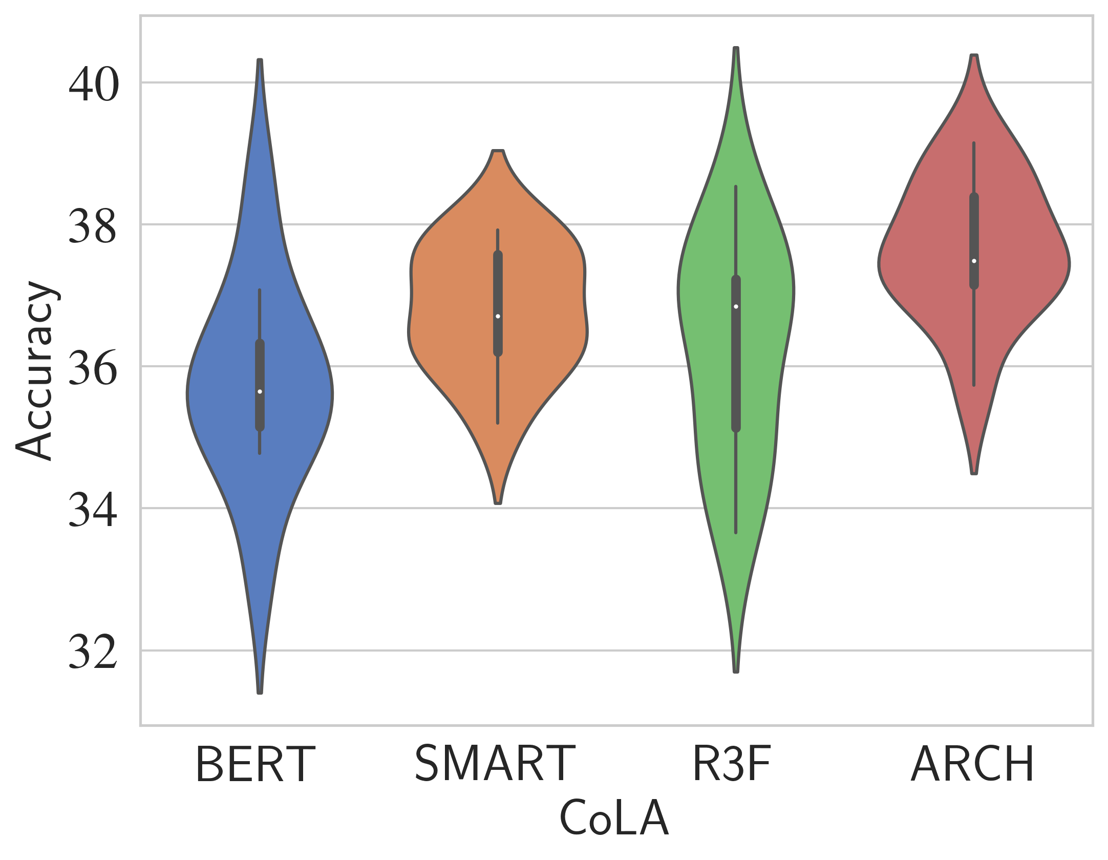
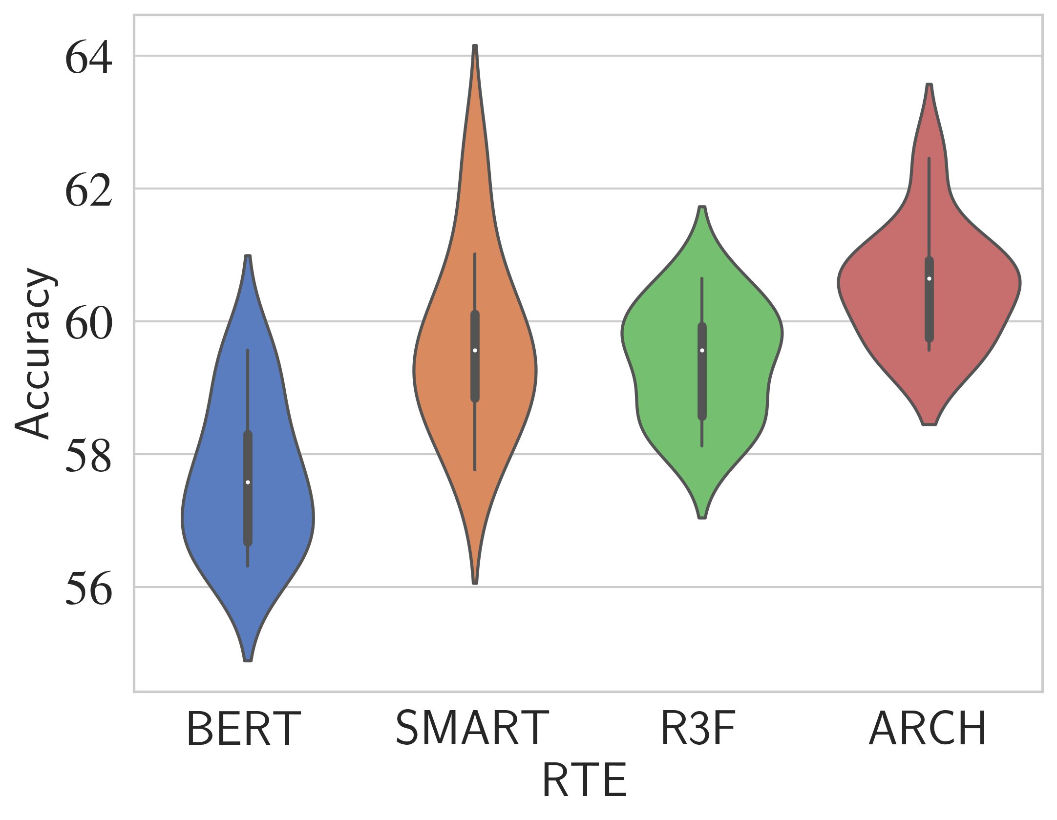
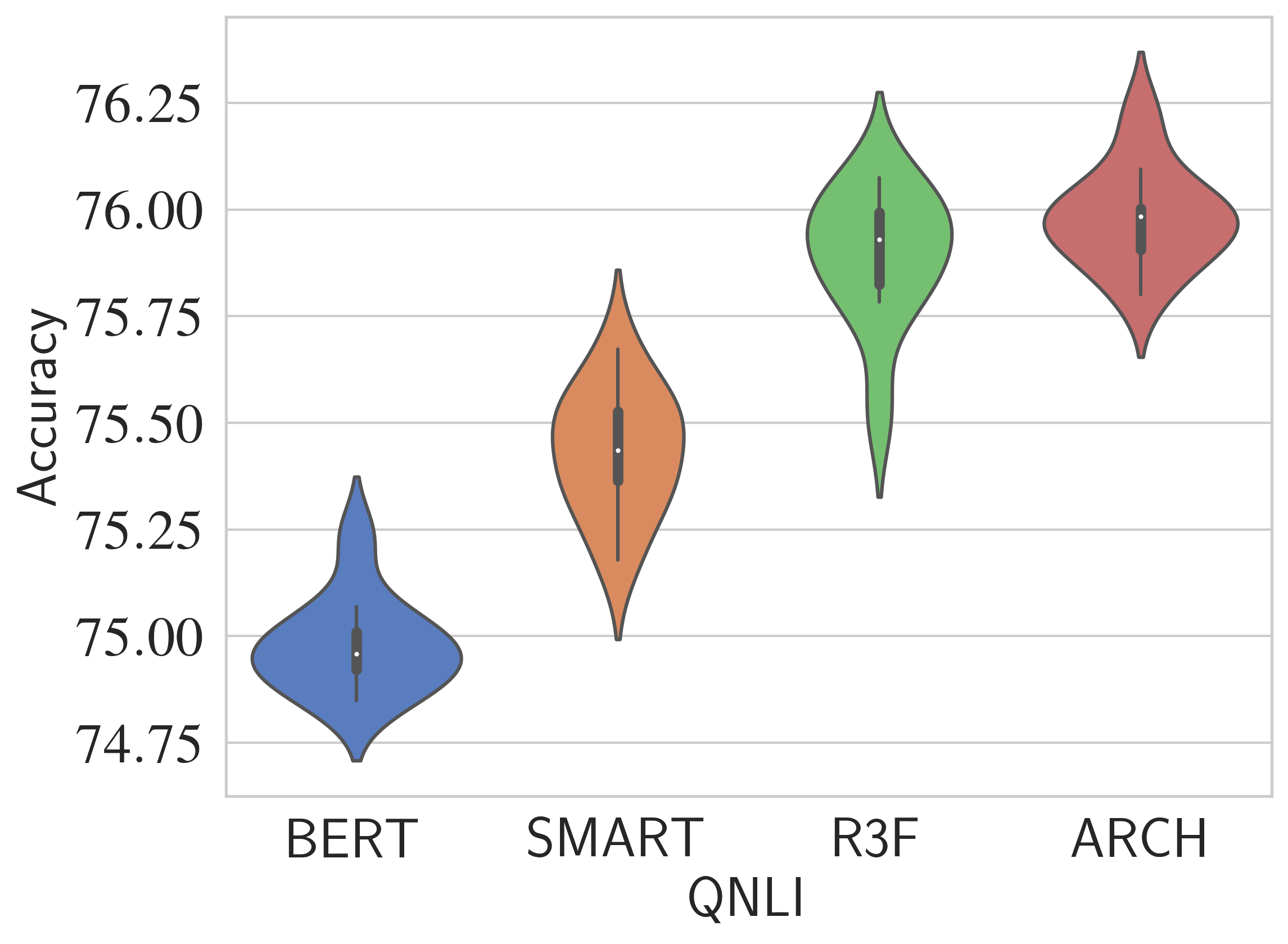
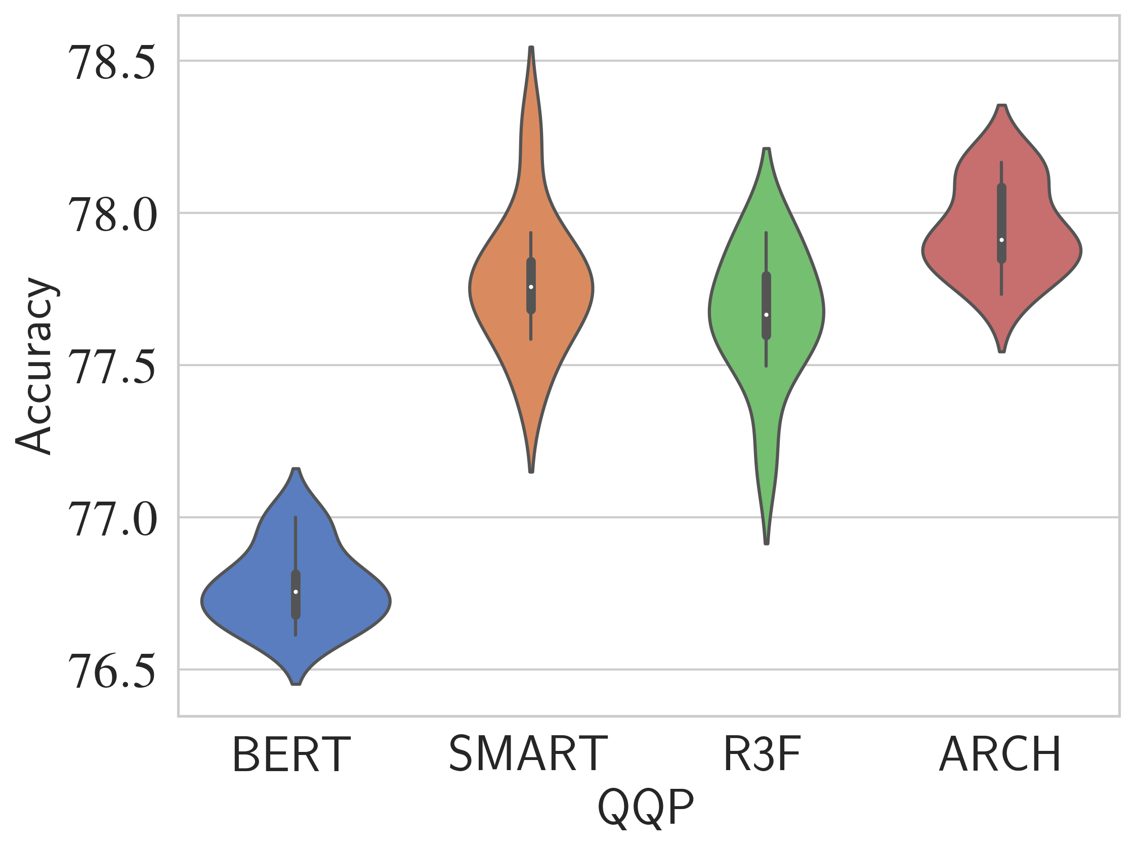
Figure 4: Probing experiments. Each violin plot is based on 10 runs with different random seeds.

5 Conclusion

We propose a new caching method to speedup the training of neural models with adversarial regularization. By reusing the generated perturbations, our proposed method significantly amortizes the computational cost of the backward passes at each iteration. Our thorough experiments show that the proposed method not only improves the computational efficiency, but also reduces the variance of the stochastic gradients, which leads to better model generalization.

Appendix A Detailed Algorithm

Input: $W$: word embedding matrix from a pre-trained model; $T$: number of training epochs; $T_{c}$: number of epochs between caching; $\alpha$: moving average parameter.

// Before training

Compute $\{v_{i}\}_{i=1}^{n}$ using Eq. 4;

Sample a cache set $\mathcal{X}\subset\{1,\cdots,n\}$;

for $i\notin\mathcal{X}$ do

       Find $\mathcal{K}_{i}\subset\mathcal{X}$ for $x_{i}$ based on cosine similarity among $\{v_{i}\}_{i=1}^{n}$;

      

end for

// During training

Initialize: Cache $\mathcal{C}=\text{dict}\{\}$;

for $t=0,\cdots T-1$ do

       for each $x_{i}\in\mathcal{B}$ in a batch $\mathcal{B}$ do

             if $t\%T_{c}==0$ then

                   Find $\delta_{i}^{t}$ for each $x_{i}$ using projected gradient ascent;

                   if $i\in\mathcal{X}$ then

                         $\mathcal{C}[x_{i}]\leftarrow\alpha\mathcal{C}[x_{i}]+(1-\alpha)\delta_{i}^{t}$;

                        

                   end if

                  

             else

                   if $i\in\mathcal{X}$ then

                         $\delta_{i}^{t}=\mathcal{C}[x_{i}]$;

                        

                   else

                         Compute $\delta_{i}^{t}$ using $\mathcal{K}_{i}$, $\mathcal{C}$, and Eq. 3;

                        

                   end if

                  

             end if

            One-step gradient descent on Eq. 2 to update model parameters;

            

       end for

      

end for

Output: Trained model.

Algorithm 3 Adversarial Regularization with Caching and Memory Saving.

Appendix B Training Details

B.1 Machine Translation Experiments

For the low-resource experiments, we use a batch size of 64k tokens. For example, when running the experiments on 4 GPUs, we set the tokens-per-GPU to be 8k, and we accumulate gradients for 2 steps. We use Adam Kingma and Ba (2015) as the optimizer, and we set $\beta=(0.9,0.98)$. The learning rate is set to be $1\times 10^{-3}$ in all the experiments. We choose the model with the best validation performance to test on the test set. Other training details are the same as Ott et al. (2019).

For the rich resource experiments, we use a batch size of 450k tokens. That is, we set tokens-per-GPU to be 7k with 8 GPUs, and we further accumulate gradients for 8 steps. We set the learning rate to be $1\times 10^{-3}\}$. For other training setups, please refer to Ott et al. (2018).

To implement our proposed method, we sample the initial perturbation from a uniform distribution. We use sentence-level $\ell_{2}$ constraints on the perturbations, and we set the perturbation strength $\epsilon=0.1$. We run a modified version of projected gradient ascent for 3 steps to compute the perturbations, and the learning rate is set to be $0.1$. Concretely, in each iteration to compute the perturbations, we apply the following update rule

$$\delta\leftarrow\Pi\left(\delta+\eta\frac{\nabla_{\delta}\ell_{v}(x,\delta,\theta)}{\left\lVert\nabla_{\delta}\ell_{v}\right\rVert_{2}}\right),$$

where $\eta$ is the learning rate and $\Pi$ denotes the projection into the $\ell_{2}$ ball. We set the number of epochs between caching to be 15, and the exponential moving average parameter $\alpha=0.01$. We cache 10% of perturbations, and we use the nearest neighbor (i.e., 1-NN) to construct uncached perturbations.

Inference settings are presented in Table 7.

	Beam	Len-Pen
En-Vi (IWSLT’15)	10	1.0
Vi-En (IWSLT’15)	15	0.3
En-De (IWSLT’14)	10	1.5
De-En (IWSLT’14)	9	1.5
En-Fr (IWSLT’16)	10	0.2
Fr-En (IWSLT’16)	10	2.0
En-De (WMT’16)	4	0.6

Table 7: Hyper-parameters for machine translation. Here, Beam is the size of beam search, and Len-Pen is the length penalty parameter during beam search.

Corpus	Task	#Train	#Dev	#Test	#Label	Metrics
Single-Sentence Classification (GLUE)
CoLA	Acceptability	8.5k	1k	1k	2	Matthews corr
SST	Sentiment	67k	872	1.8k	2	Accuracy
Pairwise Text Classification (GLUE)
MNLI	NLI	393k	20k	20k	3	Accuracy
RTE	NLI	2.5k	276	3k	2	Accuracy
QQP	Paraphrase	364k	40k	391k	2	Accuracy/F1
MRPC	Paraphrase	3.7k	408	1.7k	2	Accuracy/F1
QNLI	QA/NLI	108k	5.7k	5.7k	2	Accuracy
Text Similarity (GLUE)
STS-B	Similarity	7k	1.5k	1.4k	1	Pearson/Spearman corr

Table 8: Summary of the GLUE benchmark.

B.2 Natural Language Understanding Experiments

Statistics and descriptions of the GLUE benchmark is summarized in Table 8.

We fine-tune a pre-trained BERT_BASE model. For each task, we choose the batch size from $\{8,16,32,64,128\}$, and the learning rate from $\{5\times 10^{-5},8\times 10^{-5},1\times 10^{-4},2\times 10^{-4}\}$. We use a linear learning rate warm-up schedule for $10\%$ of the training iterations. We set the dropout rate of the task specific layer (i.e., the classification head) to be $0.1$, and the dropout rate of BERT is chosen from $\{0.0,0.1\}$. We train the model for $10$ epochs. We report the best performance on each dataset individually.

To implement the adversarial regularization method, we sample the initial perturbation from a normal distribution with mean $0$ and standard deviation $10^{-5}$. We use word-level $\ell_{\infty}$ constraints, and the perturbation strength is set to be $1.0$. We run standard projected gradient ascent to compute the perturbations, where the number of steps is chosen from $\{1,2\}$, and the learning rate is chosen from $\{10^{-4},10^{-5}\}$. Because of the limited number of training samples, we only cache the perturbations once for fine-tuning tasks. We refer to the MT-DNN code-base for other details.

References

- Aghajanyan et al. (2020) Armen Aghajanyan, Akshat Shrivastava, Anchit Gupta, Naman Goyal, Luke Zettlemoyer, and Sonal Gupta. 2020. Better fine-tuning by reducing representational collapse. arXiv preprint arXiv:2008.03156.
- Athiwaratkun et al. (2019) Ben Athiwaratkun, Marc Finzi, Pavel Izmailov, and Andrew Gordon Wilson. 2019. There are many consistent explanations of unlabeled data: Why you should average. In 7th International Conference on Learning Representations, ICLR 2019, New Orleans, LA, USA, May 6-9, 2019. OpenReview.net.
- Bahdanau et al. (2015) Dzmitry Bahdanau, Kyunghyun Cho, and Yoshua Bengio. 2015. Neural machine translation by jointly learning to align and translate. In 3rd International Conference on Learning Representations, ICLR 2015, San Diego, CA, USA, May 7-9, 2015, Conference Track Proceedings.
- Bar-Haim et al. (2006) Roy Bar-Haim, Ido Dagan, Bill Dolan, Lisa Ferro, and Danilo Giampiccolo. 2006. The second PASCAL recognising textual entailment challenge. In Proceedings of the Second PASCAL Challenges Workshop on Recognising Textual Entailment.
- Bentivogli et al. (2009) Luisa Bentivogli, Ido Dagan, Hoa Trang Dang, Danilo Giampiccolo, and Bernardo Magnini. 2009. The fifth pascal recognizing textual entailment challenge. In In Proc Text Analysis Conference (TAC’09.
- Cer et al. (2017) Daniel Cer, Mona Diab, Eneko Agirre, Iñigo Lopez-Gazpio, and Lucia Specia. 2017. SemEval-2017 task 1: Semantic textual similarity multilingual and crosslingual focused evaluation. In Proceedings of the 11th International Workshop on Semantic Evaluation (SemEval-2017), pages 1–14, Vancouver, Canada. Association for Computational Linguistics.
- Cheng et al. (2019) Yong Cheng, Lu Jiang, and Wolfgang Macherey. 2019. Robust neural machine translation with doubly adversarial inputs. In Proceedings of the 57th Annual Meeting of the Association for Computational Linguistics, pages 4324–4333, Florence, Italy. Association for Computational Linguistics.
- Dagan et al. (2006) Ido Dagan, Oren Glickman, and Bernardo Magnini. 2006. The pascal recognising textual entailment challenge. In Proceedings of the First International Conference on Machine Learning Challenges: Evaluating Predictive Uncertainty Visual Object Classification, and Recognizing Textual Entailment, MLCW’05, pages 177–190, Berlin, Heidelberg. Springer-Verlag.
- Devlin et al. (2019) Jacob Devlin, Ming-Wei Chang, Kenton Lee, and Kristina Toutanova. 2019. BERT: Pre-training of deep bidirectional transformers for language understanding. In Proceedings of the 2019 Conference of the North American Chapter of the Association for Computational Linguistics: Human Language Technologies, Volume 1 (Long and Short Papers), pages 4171–4186, Minneapolis, Minnesota. Association for Computational Linguistics.
- Dolan and Brockett (2005) William B. Dolan and Chris Brockett. 2005. Automatically constructing a corpus of sentential paraphrases. In Proceedings of the Third International Workshop on Paraphrasing (IWP2005).
- Gehring et al. (2017) Jonas Gehring, Michael Auli, David Grangier, Denis Yarats, and Yann N. Dauphin. 2017. Convolutional sequence to sequence learning. In Proceedings of the 34th International Conference on Machine Learning, ICML 2017, Sydney, NSW, Australia, 6-11 August 2017, volume 70 of Proceedings of Machine Learning Research, pages 1243–1252. PMLR.
- Giampiccolo et al. (2007) Danilo Giampiccolo, Bernardo Magnini, Ido Dagan, and Bill Dolan. 2007. The third PASCAL recognizing textual entailment challenge. In Proceedings of the ACL-PASCAL Workshop on Textual Entailment and Paraphrasing, pages 1–9, Prague. Association for Computational Linguistics.
- Goodfellow et al. (2015) Ian J. Goodfellow, Jonathon Shlens, and Christian Szegedy. 2015. Explaining and harnessing adversarial examples. In 3rd International Conference on Learning Representations, ICLR 2015, San Diego, CA, USA, May 7-9, 2015, Conference Track Proceedings.
- He et al. (2020) Pengcheng He, Xiaodong Liu, Jianfeng Gao, and Weizhu Chen. 2020. Deberta: Decoding-enhanced bert with disentangled attention. arXiv preprint arXiv:2006.03654.
- Izmailov et al. (2018) Pavel Izmailov, Dmitrii Podoprikhin, Timur Garipov, Dmitry P. Vetrov, and Andrew Gordon Wilson. 2018. Averaging weights leads to wider optima and better generalization. In Proceedings of the Thirty-Fourth Conference on Uncertainty in Artificial Intelligence, UAI 2018, Monterey, California, USA, August 6-10, 2018, pages 876–885. AUAI Press.
- Jia and Liang (2017) Robin Jia and Percy Liang. 2017. Adversarial examples for evaluating reading comprehension systems. In Proceedings of the 2017 Conference on Empirical Methods in Natural Language Processing, pages 2021–2031, Copenhagen, Denmark. Association for Computational Linguistics.
- Jiang et al. (2021) Haoming Jiang, Zhehui Chen, Yuyang Shi, Bo Dai, and Tuo Zhao. 2021. Learning to defend by learning to attack. In The 24th International Conference on Artificial Intelligence and Statistics, AISTATS 2021, April 13-15, 2021, Virtual Event, volume 130 of Proceedings of Machine Learning Research, pages 577–585. PMLR.
- Jiang et al. (2020) Haoming Jiang, Pengcheng He, Weizhu Chen, Xiaodong Liu, Jianfeng Gao, and Tuo Zhao. 2020. SMART: Robust and efficient fine-tuning for pre-trained natural language models through principled regularized optimization. In Proceedings of the 58th Annual Meeting of the Association for Computational Linguistics, pages 2177–2190, Online. Association for Computational Linguistics.
- Kingma and Ba (2015) Diederik P. Kingma and Jimmy Ba. 2015. Adam: A method for stochastic optimization. In 3rd International Conference on Learning Representations, ICLR 2015, San Diego, CA, USA, May 7-9, 2015, Conference Track Proceedings.
- Li et al. (2019) Yan Li, Ethan X Fang, Huan Xu, and Tuo Zhao. 2019. Inductive bias of gradient descent based adversarial training on separable data. arXiv preprint arXiv:1906.02931.
- Liu et al. (2020a) Xiaodong Liu, Hao Cheng, Pengcheng He, Weizhu Chen, Yu Wang, Hoifung Poon, and Jianfeng Gao. 2020a. Adversarial training for large neural language models. arXiv preprint arXiv:2004.08994.
- Liu et al. (2019a) Xiaodong Liu, Pengcheng He, Weizhu Chen, and Jianfeng Gao. 2019a. Multi-task deep neural networks for natural language understanding. In Proceedings of the 57th Annual Meeting of the Association for Computational Linguistics, pages 4487–4496, Florence, Italy. Association for Computational Linguistics.
- Liu et al. (2020b) Xiaodong Liu, Yu Wang, Jianshu Ji, Hao Cheng, Xueyun Zhu, Emmanuel Awa, Pengcheng He, Weizhu Chen, Hoifung Poon, Guihong Cao, and Jianfeng Gao. 2020b. The Microsoft toolkit of multi-task deep neural networks for natural language understanding. In Proceedings of the 58th Annual Meeting of the Association for Computational Linguistics: System Demonstrations, pages 118–126, Online. Association for Computational Linguistics.
- Liu et al. (2019b) Yinhan Liu, Myle Ott, Naman Goyal, Jingfei Du, Mandar Joshi, Danqi Chen, Omer Levy, Mike Lewis, Luke Zettlemoyer, and Veselin Stoyanov. 2019b. Roberta: A robustly optimized bert pretraining approach. arXiv preprint arXiv:1907.11692.
- Madry et al. (2018) Aleksander Madry, Aleksandar Makelov, Ludwig Schmidt, Dimitris Tsipras, and Adrian Vladu. 2018. Towards deep learning models resistant to adversarial attacks. In 6th International Conference on Learning Representations, ICLR 2018, Vancouver, BC, Canada, April 30 - May 3, 2018, Conference Track Proceedings. OpenReview.net.
- Min et al. (2020) Yifei Min, Lin Chen, and Amin Karbasi. 2020. The curious case of adversarially robust models: More data can help, double descend, or hurt generalization. arXiv preprint arXiv:2002.11080.
- Miyato et al. (2017) Takeru Miyato, Andrew M. Dai, and Ian J. Goodfellow. 2017. Adversarial training methods for semi-supervised text classification. In 5th International Conference on Learning Representations, ICLR 2017, Toulon, France, April 24-26, 2017, Conference Track Proceedings. OpenReview.net.
- Nie et al. (2020) Yixin Nie, Adina Williams, Emily Dinan, Mohit Bansal, Jason Weston, and Douwe Kiela. 2020. Adversarial NLI: A new benchmark for natural language understanding. In Proceedings of the 58th Annual Meeting of the Association for Computational Linguistics, pages 4885–4901, Online. Association for Computational Linguistics.
- Ott et al. (2019) Myle Ott, Sergey Edunov, Alexei Baevski, Angela Fan, Sam Gross, Nathan Ng, David Grangier, and Michael Auli. 2019. fairseq: A fast, extensible toolkit for sequence modeling. In Proceedings of the 2019 Conference of the North American Chapter of the Association for Computational Linguistics (Demonstrations), pages 48–53, Minneapolis, Minnesota. Association for Computational Linguistics.
- Ott et al. (2018) Myle Ott, Sergey Edunov, David Grangier, and Michael Auli. 2018. Scaling neural machine translation. In Proceedings of the Third Conference on Machine Translation: Research Papers, pages 1–9, Brussels, Belgium. Association for Computational Linguistics.
- Paszke et al. (2019) Adam Paszke, Sam Gross, Francisco Massa, Adam Lerer, James Bradbury, Gregory Chanan, Trevor Killeen, Zeming Lin, Natalia Gimelshein, Luca Antiga, Alban Desmaison, Andreas Köpf, Edward Yang, Zachary DeVito, Martin Raison, Alykhan Tejani, Sasank Chilamkurthy, Benoit Steiner, Lu Fang, Junjie Bai, and Soumith Chintala. 2019. Pytorch: An imperative style, high-performance deep learning library. In Advances in Neural Information Processing Systems 32: Annual Conference on Neural Information Processing Systems 2019, NeurIPS 2019, December 8-14, 2019, Vancouver, BC, Canada, pages 8024–8035.
- Peters et al. (2018) Matthew Peters, Mark Neumann, Mohit Iyyer, Matt Gardner, Christopher Clark, Kenton Lee, and Luke Zettlemoyer. 2018. Deep contextualized word representations. In Proceedings of the 2018 Conference of the North American Chapter of the Association for Computational Linguistics: Human Language Technologies, Volume 1 (Long Papers), pages 2227–2237, New Orleans, Louisiana. Association for Computational Linguistics.
- Post (2018) Matt Post. 2018. A call for clarity in reporting BLEU scores. In Proceedings of the Third Conference on Machine Translation: Research Papers, pages 186–191, Brussels, Belgium. Association for Computational Linguistics.
- Radford et al. (2019) Alec Radford, Jeffrey Wu, Rewon Child, David Luan, Dario Amodei, and Ilya Sutskever. 2019. Language models are unsupervised multitask learners. OpenAI blog, 1(8):9.
- Raghunathan et al. (2020) Aditi Raghunathan, Sang Michael Xie, Fanny Yang, John C. Duchi, and Percy Liang. 2020. Understanding and mitigating the tradeoff between robustness and accuracy. In Proceedings of the 37th International Conference on Machine Learning, ICML 2020, 13-18 July 2020, Virtual Event, volume 119 of Proceedings of Machine Learning Research, pages 7909–7919. PMLR.
- Rajpurkar et al. (2016) Pranav Rajpurkar, Jian Zhang, Konstantin Lopyrev, and Percy Liang. 2016. SQuAD: 100,000+ questions for machine comprehension of text. In Proceedings of the 2016 Conference on Empirical Methods in Natural Language Processing, pages 2383–2392, Austin, Texas. Association for Computational Linguistics.
- Sato et al. (2019) Motoki Sato, Jun Suzuki, and Shun Kiyono. 2019. Effective adversarial regularization for neural machine translation. In Proceedings of the 57th Annual Meeting of the Association for Computational Linguistics, pages 204–210, Florence, Italy. Association for Computational Linguistics.
- Shafahi et al. (2019) Ali Shafahi, Mahyar Najibi, Amin Ghiasi, Zheng Xu, John P. Dickerson, Christoph Studer, Larry S. Davis, Gavin Taylor, and Tom Goldstein. 2019. Adversarial training for free! In Advances in Neural Information Processing Systems 32: Annual Conference on Neural Information Processing Systems 2019, NeurIPS 2019, December 8-14, 2019, Vancouver, BC, Canada, pages 3353–3364.
- Shen et al. (2020) Qianli Shen, Yan Li, Haoming Jiang, Zhaoran Wang, and Tuo Zhao. 2020. Deep reinforcement learning with robust and smooth policy. In Proceedings of the 37th International Conference on Machine Learning, ICML 2020, 13-18 July 2020, Virtual Event, volume 119 of Proceedings of Machine Learning Research, pages 8707–8718. PMLR.
- Socher et al. (2013) Richard Socher, Alex Perelygin, Jean Wu, Jason Chuang, Christopher D. Manning, Andrew Ng, and Christopher Potts. 2013. Recursive deep models for semantic compositionality over a sentiment treebank. In Proceedings of the 2013 Conference on Empirical Methods in Natural Language Processing, pages 1631–1642, Seattle, Washington, USA. Association for Computational Linguistics.
- Szegedy et al. (2014) Christian Szegedy, Wojciech Zaremba, Ilya Sutskever, Joan Bruna, Dumitru Erhan, Ian J. Goodfellow, and Rob Fergus. 2014. Intriguing properties of neural networks. In 2nd International Conference on Learning Representations, ICLR 2014, Banff, AB, Canada, April 14-16, 2014, Conference Track Proceedings.
- Vaswani et al. (2017) Ashish Vaswani, Noam Shazeer, Niki Parmar, Jakob Uszkoreit, Llion Jones, Aidan N. Gomez, Lukasz Kaiser, and Illia Polosukhin. 2017. Attention is all you need. In Advances in Neural Information Processing Systems 30: Annual Conference on Neural Information Processing Systems 2017, December 4-9, 2017, Long Beach, CA, USA, pages 5998–6008.
- Wang et al. (2019a) Alex Wang, Amanpreet Singh, Julian Michael, Felix Hill, Omer Levy, and Samuel R. Bowman. 2019a. GLUE: A multi-task benchmark and analysis platform for natural language understanding. In 7th International Conference on Learning Representations, ICLR 2019, New Orleans, LA, USA, May 6-9, 2019. OpenReview.net.
- Wang et al. (2019b) Dilin Wang, ChengYue Gong, and Qiang Liu. 2019b. Improving neural language modeling via adversarial training. In Proceedings of the 36th International Conference on Machine Learning, ICML 2019, 9-15 June 2019, Long Beach, California, USA, volume 97 of Proceedings of Machine Learning Research, pages 6555–6565. PMLR.
- Warstadt et al. (2019) Alex Warstadt, Amanpreet Singh, and Samuel R. Bowman. 2019. Neural network acceptability judgments. Transactions of the Association for Computational Linguistics, 7:625–641.
- Williams et al. (2018) Adina Williams, Nikita Nangia, and Samuel Bowman. 2018. A broad-coverage challenge corpus for sentence understanding through inference. In Proceedings of the 2018 Conference of the North American Chapter of the Association for Computational Linguistics: Human Language Technologies, Volume 1 (Long Papers), pages 1112–1122, New Orleans, Louisiana. Association for Computational Linguistics.
- Wolf et al. (2020) Thomas Wolf, Lysandre Debut, Victor Sanh, Julien Chaumond, Clement Delangue, Anthony Moi, Pierric Cistac, Tim Rault, Remi Louf, Morgan Funtowicz, Joe Davison, Sam Shleifer, Patrick von Platen, Clara Ma, Yacine Jernite, Julien Plu, Canwen Xu, Teven Le Scao, Sylvain Gugger, Mariama Drame, Quentin Lhoest, and Alexander Rush. 2020. Transformers: State-of-the-art natural language processing. In Proceedings of the 2020 Conference on Empirical Methods in Natural Language Processing: System Demonstrations, pages 38–45, Online. Association for Computational Linguistics.
- Zhu et al. (2020) Chen Zhu, Yu Cheng, Zhe Gan, Siqi Sun, Tom Goldstein, and Jingjing Liu. 2020. Freelb: Enhanced adversarial training for natural language understanding. In 8th International Conference on Learning Representations, ICLR 2020, Addis Ababa, Ethiopia, April 26-30, 2020. OpenReview.net.
- Zuo et al. (2021) Simiao Zuo, Chen Liang, Haoming Jiang, Xiaodong Liu, Pengcheng He, Jianfeng Gao, Weizhu Chen, and Tuo Zhao. 2021. Adversarial training as stackelberg game: An unrolled optimization approach. arXiv preprint arXiv:2104.04886.