A Massively Multilingual Analysis of Cross-linguality
in Shared Embedding Space

Abstract

In cross-lingual language models, representations for many different languages live in the same space. Here, we investigate the linguistic and non-linguistic factors affecting sentence-level alignment in cross-lingual pretrained language models for 101 languages and 5,050 language pairs. Using BERT-based LaBSE and BiLSTM-based LASER as our models, and the Bible as our corpus, we compute a task-based measure of cross-lingual alignment in the form of bitext retrieval performance, as well as four intrinsic measures of vector space alignment and isomorphism. We then examine a range of linguistic, quasi-linguistic, and training-related features as potential predictors of these alignment metrics. The results of our analyses show that word order agreement and agreement in morphological complexity are two of the strongest linguistic predictors of cross-linguality. We also note in-family training data as a stronger predictor than language-specific training data across the board. We verify some of our linguistic findings by looking at the effect of morphological segmentation on English-Inuktitut alignment, in addition to examining the effect of word order agreement on isomorphism for 66 zero-shot language pairs from a different corpus. We make the data and code for our experiments publicly available.

1 Introduction

Cross-lingual language models are polyglots insofar as they house representations for many different languages in the same space. But to what extent are they good polyglots? The answer depends, in part, on how well-aligned and isomorphic the representations are, and not all language pairs are equally well-aligned. What determines the quality of the alignment? Are language pairs from the same family (e.g., Spanish and French) better aligned than languages from two unrelated families (e.g., Japanese and Swahili)? Are languages which are geographically closer or share an alphabet better aligned? How do factors from linguistic typology (like word order and morphological marking) affect alignment?

Recent work has looked at the typological and training-related factors affecting cross-lingual alignment in monolingual embedding space Vulić et al. (2020); Dubossarsky et al. (2020), assessed the cross-linguality of pretrained language models using probing tasks and downstream performance measures Conneau et al. (2020); Wu and Dredze (2019, 2020); Pires et al. (2019); Groenwold et al. (2020), and probed Transformer models Wolf et al. (2020) for linguistic structure (see Rogers et al. 2020 for an overview of over 150 studies). However, a gap in the research exists regarding the following question: What are the linguistic, quasi-linguistic, and training-related factors determining the cross-linguality of sentence representations in shared embedding space, and what are the relative weights of these factors?

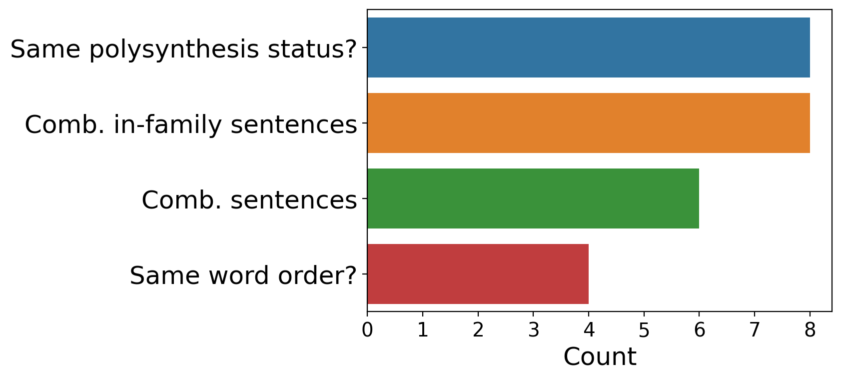
Figure 1: A look at some of the strongest features for predicting cross-linguality, according to their number of occurrences in best-feature regression searches across all our dependent variables (see Section 6.2).

We argue, that given the importance of alignment in multilingual model performance, gaining fundamental insight into what affects inter-language alignment and isomorphism—specifically by exploring which linguistic factors matter for inter-language alignment—will make it possible to leverage existing information on linguistic typology to improve alignment (and thereby task performance) for low-resource languages.

Our contributions are as follows:

• We provide a characterization of cross-linguality for 101 languages (29 language families) in two massively multilingual sentence embedding models with different architectures (LaBSE and LASER), attacking the question from the vantage of vector space analysis—using four measures of alignment and isomorphism—and downstream task performance (namely bitext retrieval).

• We present over a dozen linguistic, quasi-linguistic, and training-related factors as potential predictors of cross-linguality, and examine their relationship with the above metrics using diverse statistical analyses.

• We uncover novel and pronounced effects of morphology agreement and word order agreement on cross-linguality, demonstrate the importance of in-family training data in ensuring multilinguality, and validate our linguistic findings with two empirical case studies on low-resource languages.

2 Related Work

Various studies have assessed the cross-linguality of pretrained language models. Recent efforts have approached this question via performance on an array of downstream NLP tasks Conneau et al. (2020); Wu and Dredze (2019, 2020); Karthikeyan et al. (2020); Pires et al. (2019); Groenwold et al. (2020), and others have proposed methods for better cross-lingual alignment in light of systematic cross-lingual deficiencies Zhang et al. (2019); Xia et al. (2021). Our study hews closest methodologically to Vulić et al. (2020) and Dubossarsky et al. (2020), who investigate the determinants of cross-lingual isomorphism using monolingual fastText embeddings Bojanowski et al. (2016); Joulin et al. (2016); Mikolov et al. (2013).

Findings from these studies have been mixed, but some patterns emerge. Pires et al. (2019) and Conneau et al. (2020) find that cross-lingual transfer works best between typologically similar language pairs, in particular between languages that share word order features. Wu and Dredze (2019) approach cross-linguality by focusing on zero-shot cross-lingual transfer in mBERT, and show that each mBERT layer retains language-specific information and that token overlap correlates with cross-lingual performance. Wu and Dredze (2020) home in on low-resource languages, finding that they often fail to reap the benefits of massively multilingual joint training but that their performance can be boosted by providing similar-language training data. Somewhat contrary to others’ results (including ours), Karthikeyan et al. (2020) find that lexical overlap factors in negligibly to cross-lingual transfer, while the depth of the network is integrally important. Vulić et al. (2020) and Dubossarsky et al. (2020) look at how typological features, training-related factors, and measures of vector space isomorphism predict cross-lingual performance between monolingual word embeddings. Vulić et al. (2020) find in their experiments that cross-lingual performance depends mostly on training data and regimes, while Dubossarsky et al. (2020) see more mixed results from their experiments: They show that linguistic typology is important, but not deterministic, for predicting cross-lingual performance.

Our work not only replicates these findings for monolingual spaces in the multilingual embedding space (e.g. on word order similarity, related training data, typological distance, subword overlap), but extends that work through: (1) The scale (101 languages, 5,050 language pairs in the main analysis); (2) The quantity and diversity of predictors (13 linguistic, quasi-linguistic, and training-related features); (3) The models (cross-lingual sentence encoders with different architectures); and (4) The analytic methods (a blend of prediction-based and classical statistical techniques, supplemented by performance-based case studies on extremely low-resource languages).

3 Bible Corpus

The source of the bitexts we evaluate on is the superparallel Bible corpus from Christodouloupoulos and Steedman (2014), whence we gather texts for 101 languages and bitexts for 5,050 language pairs. We evaluate on the Books of Matthew and John in the New Testament separately and average the results, as these parts are available for all 101 languages. In doing so, we avoid the pitfalls of relying on a single set of bitexts for our analysis. Each document contains 800-1000 sentences.

4 Measures of Cross-lingual Alignment & Isomorphism

We formulate alignment metrics in two distinct ways: over language pairs and over individual languages. The latter group is computed from the former by averaging over all pairs in which a language appears. For example, to derive the average F1-score for Chinese, we average over the F1-scores for Chinese-German, Chinese-Amuzgo, etc.

Some metrics we use are measures of vector subspace isomorphism (i.e. those examined in Dubossarsky et al. 2020), while others are measures of alignment (namely those pertaining to bitext retrieval). Vector spaces may be isomorphic without being well-aligned, so we quantify multilinguality in diverse ways.

4.1 Bitext Retrieval Task

The bitext retrieval task consists of finding all sentences in a paired set of documents that are translations of each other. This process can be carried out between two comparable corpora, such as Wikipedia (“bitext mining”), but we use the 5,050 bitexts collected from the Bible corpus. We mine in two directions: for each sentence in document $\mathcal{X}$, we find a match in document $\mathcal{Y}$, and vice-versa. We then take the intersection of those two searches, which has proven to be a useful heuristic Artetxe and Schwenk (2019a); Jones and Wijaya (2021). Note that this task can be thought of as the sentence-level analog to the bilingual lexicon induction (BLI) task used in Vulić et al. (2020) and Dubossarsky et al. (2020).

Task performance

Margin scoring, introduced by Artetxe and Schwenk (2019a), has shown success on the bitext retrieval task Schwenk et al. (2021, 2019); Keung et al. (2021); Tran et al. (2020); Fan et al. (2020); Jones and Wijaya (2021). Margin score may be thought of as “relativized” cosine similarity, in that it selects vectors that “stand out” most among their neighbors in terms of proximity, rather than ones that are simply closest together. The method requires initially finding the $k$-nearest neighbors of each source and target sentence, which we do efficiently with Faiss Johnson et al. (2017a). The sentence pair $(x,y)$ is then chosen to maximize the margin score between $x$ and $y$, namely

$$\begin{split}&\mathrm{score_{margin}}(x,y)=\\ &\frac{2k\cos{(x,y)}}{\sum_{z\in NN_{k}(x)}{\cos{(x,z)}}+\sum_{z\in NN_{k}(y)}{\cos{(y,z)}}}\end{split}$$

After retrieving sentence pairs in both directions and keeping the intersection, we compute standard F1-score against ground-truth alignments.

Average margin score

We also introduce a novel alignment metric in the form of the average margin score across ground-truth sentence alignments. Namely, given aligned sentence embedding matrices $\mathcal{X}$ and $\mathcal{Y}$ with $N$ embeddings each, the average margin score is computed as

$$\begin{split}&\mathrm{margin_{avg}}(\mathcal{X},\mathcal{Y})=\\ &\frac{1}{N}\sum_{i=1}^{N}{\mathrm{score_{margin}}(\mathcal{X}_{i},\mathcal{Y}_{i}})\mid\mathcal{X},\mathcal{Y}\in\mathbb{R}^{N\times emb\_dim}\end{split}$$

This provides a continuous measure of cross-lingual alignment that is correlated with, but not equivalent to, the F1-score on this task.

4.2 Approximate Isomorphism

Vulić et al. (2020) and Dubossarsky et al. (2020) introduce various ways of quantifying the degree of isomorphism between two vector spaces, of which we use three. Note that unlike Vulić et al. (2020) and Dubossarsky et al. (2020), who investigate isomorphism between monolingual spaces, we examine cross-lingual isomorphism within shared embedding space. These metrics thus technically quantify vector subspace isomorphism, where each subspace comprises embeddings in a particular language.

Gromov-Hausdorff distance

The Hausdorff distance between two metric spaces $\mathcal{X}$ and $\mathcal{Y}$, given by

$$\mathcal{H}(\mathcal{X},\mathcal{Y})=\max[{\sup_{x\in\mathcal{X}}{\inf_{y\in\mathcal{Y}}}{d(x,y),\sup_{y\in\mathcal{Y}}{\inf_{x\in\mathcal{X}}}{d(x,y)}}}]$$

intuitively measures the worst-case distance between the nearest neighbors of $\mathcal{X}$ and $\mathcal{Y}$ Vulić et al. (2020). The Gromov-Hausdorff distance then minimizes this distance over all isometric transforms $f$ and $g$:

$$\mathcal{GH}(\mathcal{X},\mathcal{Y})=\inf_{f,g}{\mathcal{H}(f(\mathcal{X}),g(\mathcal{Y}))}$$

In practice, the Gromov-Hausdorff distance is approximated by computing the Bottleneck distance between $\mathcal{X}$ and $\mathcal{Y}$ Dubossarsky et al. (2020); Chazal et al. (2009).

Singular value gap

Given cross-lingual aligned sentence embeddings stored in matrices $\mathcal{X}$ and $\mathcal{Y}$, each with $n$ singular values $\sigma_{1},\sigma_{2},...,\sigma_{n}$ sorted in descending order, the singular value gap Dubossarsky et al. (2020) between $\mathcal{X}$ and $\mathcal{Y}$ is defined as

$$\mathrm{SVG}(\mathcal{X},\mathcal{Y})=\sum_{i=1}^{n}{(\log{\sigma_{i}^{\mathcal{X}}}-\log{\sigma_{i}^{\mathcal{Y}})^{2}}}$$

Effective condition number

The effective condition number Dubossarsky et al. (2020) of a matrix $\mathcal{X}$ intuitively captures the extent to which small perturbations in $\mathcal{X}$ are amplified as a result of arbitrary transformations $\phi({\mathcal{X}})$. The lower the (effective) condition number of an embedding space, the more robust it is to transformations (e.g. transfer functions mapping one embedding space to another).

Dubossarsky et al. (2020) reason that monolingual embedding spaces with lower (effective) condition numbers map better to other spaces. They further show that taking the harmonic mean of the effective condition numbers (ECOND-HM) of two embedding spaces provides a reliable measure of approximate isomorphism between those spaces. We use ECOND-HM in a similar fashion to gauge the approximate isomorphism, or “mappability,” of cross-lingual embedding subspaces, where a lower ECOND-HM indicates greater isomorphism.

5 Predictors

5.1 Linguistic Features

Similarly to the alignment metrics, we define separate sets of features pertaining to language pairs and pertaining to individual languages. We take note of this in our descriptions below.

Phylogeny

For individual languages (all languages in the New Testament corpus), we use both language family and subfamily as categorical features. For language pairs, we define two binary variables: same family and same subfamily, corresponding to whether two languages are in the same family or subfamily, respectively.

We include subfamily as a feature in order to investigate finer-grained typological and phylogenetic differences that may affect cross-lingual alignment or isomorphism.

Word order typology

For individual languages, we include basic word order as a feature, using the canonical six-way taxonomy (i.e. permutations of {S, O, V}). For language pairs, we define binary feature same word order analogously to the binary features above. We consult the WALS database Dryer and Haspelmath (2013) and Glottolog Hammarström et al. (2020) to assign dominant word orders.

Morphological typology

Though it is possible to make fine-grained distinctions in morphological typology in theory, we simply draw a binary distinction between languages that are widely considered polysynthetic (mostly Amerindian languages) and all other languages. Even more so than word order, morphological complexity is gradient (Cotterell et al., 2019). But we argue that polysynthetic languages pose a unique challenge for NLP systems and so perform one-vs-all binary coding such that individual languages are associated with a polysynthesis status and language pairs are associated with the feature same polysynthesis status. We classify 17 languages in the corpus as polysynthetic.

Typological distance

We also use typological word vectors from lang2vec Malaviya et al. (2017), based on the URIEL typological database Littell et al. (2017) to compute the distance between languages on the basis of aggregated linguistic features. Specifically, we compute:

1. Syntactic distance using KNN-based syntax vectors

2. Phonological distance using KNN-based phonology vectors

3. Inventory distance using KNN-based phonological inventory vectors (distinct from phonological distance)

4. Geographic distance using geographic location vectors

All distances are computed as cosine distances.

Character- & token-level overlap

The standard Jaccard similarity coefficient quantifies the overlap between sets $\mathbf{A}$ and $\mathbf{B}$ as:

$$J(\mathbf{A},\mathbf{B})=\frac{|\mathbf{A}\bigcap\mathbf{B}|}{|\mathbf{A}\bigcup\mathbf{B}|}$$

However, this measure fails to take into account the frequency of the items (here, characters) in each set. What we really want is the weighted, or multiset, version of the Jaccard coefficient. For our purposes, it suffices to reformulate $J$ as:

$$\begin{split}J_{M}(\mathcal{X},\mathcal{Y})=\frac{|chr(\mathcal{X}_{M})\bigcap chr(\mathcal{Y}_{M})|}{|chr(\mathcal{X}_{M})\bigcup chr(\mathcal{Y}_{M})|}\forall\mathcal{X},\mathcal{Y}\in\mathbf{C}\end{split}$$

where $chr(\mathcal{D}_{M})$ represents the multiset of characters in document $\mathcal{D}$, and $\mathbf{C}$ is the corpus of bitexts we’re working with. For convenience and to avoid redundancy, we compute $J_{M}$ (character-level overlap) only on aligned texts in the Book of Matthew. Token-level overlap is computed analogously, using the wordpiece Wu et al. (2016) tokenization method employed by LaBSE. This measure is only computed on texts in the Book of John.

5.2 Training-related Features

The aim of our analysis is to understand the effect of each of the previously described features on cross-lingual alignment and isomorphism when training factors are controlled for. To this end, we control for several (pre)training data quantities for the models tested.

First, we account for language-specific training data for individual languages. However, we also account for combined language-specific training data for language pairs, i.e. the amount of data for $x$ plus the amount of data for $y$, where $(x,y)$ is a language pair. We then take it a step further and record (combined) in-family training data and (combined) in-subfamily training data, taking inspiration from gains made using transfer languages for cross-lingual learning Johnson et al. (2017b); Littell et al. (2019); Lin et al. (2019).

By considering these broader training-related statistics, we are able to better control for and observe the role higher-level typological information (e.g. at the family or subfamily level) plays in training these models.

6 Analysis

6.1 Simple Correlations

Training data

We first look at simple correlations between the training data quantities and the dependent variables (measures of alignment/isomorphism). Results for language pairs are given across all dependent variables for LaBSE and LASER in Table 1. The most striking observation is that combined in-family training data is more highly correlated with the dependent variables than simple combined data or combined in-subfamily data for all dependent variables, for both LaBSE and LASER ($0.12\leq|r|\leq 0.57$). At the individual language level, results are similar (i.e. in-family data is most significant), but with weaker correlations across the board ($0.02\leq|r|\leq 0.18$). Based on these preliminary results, we highlight combined in-family training data as a moderately strong predictor of alignment/isomorphism for a given language pair, one that is in fact better than language-specific data for making predictions about massively multilingual sentence models.

(Quasi)-linguistic Features

Among the predictors, there were several noteworthy correlations. Same family was moderately correlated with better alignment/isomorphism in both LaBSE and LASER (generally $0.2<|r|<0.45$), while same subfamily was somewhat less correlated. This informs us as to the level at which related-language data is useful for building massively cross-lingual models. Same word order and same polysynthesis status had comparable relationships with the dependent variables as did same family. Token-level overlap was moderately but inconsistently correlated with dependent variables ($\approx 0.05<|r|<0.5$), while character-level overlap was somewhat more weakly correlated. The typological distance features were weakly but non-negligibly correlated with dependent variables ($\approx 0.1<|r|<0.3$), with one outlier (syntactic distance was correlated with $r=-0.44$ with bitext retrieval F1-score for LASER). The typological distance features were moderately correlated with one another.

	Comb. sentences	Comb. in-family	Comb. in-subfamily
Metric		sentences	sentences
	LaBSE LASER	LaBSE LASER	LaBSE LASER
Bitext retrieval (F1)	0.34       0.13	0.49        0.57	0.46       0.35
Avg. margin score	0.30      -0.03	0.40       0.14	0.37       0.07
SVG	-0.08      -0.04	-0.12      -0.13	-0.11      -0.08
ECOND-HM	-0.03       0.07	-0.38      -0.30	-0.31      -0.11
Gromov-Hausdorff dist.	-0.13      -0.07	-0.20      -0.20	-0.18      -0.10

Table 1: Correlations (Pearson’s $r$) between training data quantities and alignment/isomorphism metrics for language pairs.

6.2 Feature Search and Ablation

Exhaustive Feature Selection

We look at the optimal set of language-pair-specific features for predicting the five measures of alignment and isomorphism. To do so, we perform exhaustive feature search on linear regression models with each of the dependent variables being used separately as the regressand. To counter overfitting, we run ten-fold cross-validation and use adjusted $r^{2}$ as the fit criterion, which further penalizes for additional predictors. Adjusted $r^{2}$ is given by

$$r_{adj}^{2}=1-\frac{(1-r^{2})(n-1)}{n-k-1}$$

where $n$ is the sample size (here, $n=5050$) and $k$ is the number of predictors in the model (here, $1\leq k\leq 13$). In total, we fit $2^{|F|}=2^{13}=8192$ regression models for LaBSE and LASER separately, where $F$ is our feature space.

For interpretability, we aggregate results by tallying the frequency with which each feature appears in a best-feature list—giving model-specific results as well as combined results—which are displayed in Table 2. For the combined (LaBSE+LASER) results, same polysynthesis status and combined in-family sentences are tied as the most popular predictors, with 8/10 best-feature list appearances each. Next in line for combined results is combined sentences (6 appearances), followed by a three-way tie between same word order, token-level overlap, and geographic distance (3 appearances). Results are very similar for each model separately, although same word order is tied for second place for LASER, alongside syntactic distance and phonological distance (3 appearances).

These results show that certain (quasi)-linguistic features (in particular, same polysynthesis status and same word order) are not redundant predictors in the presence of training data quantities. Our next analysis examines individual features in terms of the size of their marginal contribution to the regression model fit.

Single-step Regression

To appraise the marginal contribution of each feature to overall regression fit, we perform a single-step ablation experiment where we eliminate features from a full-feature model one at a time. We fit a regression model with all 13 features using ten-fold cross-validation and obtain a baseline $r^{2}_{adj_{\texttt{bsl}}}$. We then compute

$$\Delta r_{adj_{\texttt{f}}}^{2}=r^{2}_{adj_{\texttt{bsl}}}-r^{2}_{adj_{\texttt{abl}}},$$

$$r^{2}_{adj_{\texttt{abl}}}\mathrel{\stackon[1.5pt]{=}{\stretchto{\scalerel*[\widthof{=}]{\wedge}{\rule{4.30554pt}{12.91663pt}}}{0.5ex}}}F\setminus\{f\}\forall f\in$$

The value of $\Delta r_{adj_{\texttt{f}}}^{2}$ is computed for all features $f$ and with each dependent variable separately as the regressand, for LaBSE and LASER separately. To aggregate results, we look at the average rank of each feature according to the ablation experiment, across all five dependent variables.

The top three results for LaBSE and LASER are given in Table 3. For LaBSE, same polysynthesis status and combined sentences are tied as the features with the highest predictive contributions (average rank = 2.4), followed by combined in-family sentences. For LASER, combined in-family sentences tops the list (average rank = 2.4), followed by same polysynthesis status and same word order. The results of this experiment are similar, but not identical, to those of the previous experiment. They support the same basic conclusion: training data is important, but so are agreement in word order and agreement in morphological complexity, among other features. If training data were a sufficient predictor alone, then removing the aforementioned features from the regression model would either increase the fit or do nothing, which clearly isn’t the case.

		Count
Feature	LaBSE	LASER	Total
Comb. sentences	4	2	6
Comb. in-family sentences	4	4	8
Comb. in-subfamily sentences	1	1	2
Same word order	1	3	4
Same polysynthesis status	4	4	8
Same family	1	2	3
Same subfamily	1	1	2
Token overlap	2	2	4
Character overlap	0	0	0
Geographic distance	2	2	4
Syntactic distance	0	3	3
Phonological distance	0	3	3
Inventory distance	0	0	0

Table 2: The number of times each of the features appeared in the best-feature lists across the five alignment metrics. The top three results (including ties) in each group are in bold.

LaBSE
1. Same polysynthesis status	2.4
2. Combined sentences	2.4
3. Combined in-family sentences	3.6

LASER
1. Combined in-family sentences	2.4
2. Same polysynthesis status	3.4
3. Same word order	3.8

Table 3: Features with the top three average rankings in the single-step regression ablation experiment. Rankings are based on a feature’s marginal predictive contribution relative to other features, and were averaged across all five alignment metrics.

6.3 Controlling for Training Data

While the previous experiments center around prediction of the dependent variables, we bolster our analysis with classical statistical methods that aim to explicitly control for covariates. Since we’re dealing with categorical features, we use ANCOVA (ANalysis of COVAriance).

ANCOVA

We run ANCOVAs separately for LaBSE and LASER and for each of the five dependent variables. We examine the language-pair-specific features, and look at same word order and same polysynthesis status separately as our “between” variables, and combined sentences, combined in-family sentences, and combined in-subfamily sentences as our three covariates. Overall, same word order had a statistically significant ($p<<0.05$) effect for 8/10 ANCOVAs, though effect sizes ($\eta_{p}^{2}$) were generally smallCohen (1988). Same polysynthesis status had a statistically significant effect for 10/10 ANCOVAs, with effect sizes being definitively small except for F1-score and ECOND-HM/average margin score ($\eta_{p}^{2}\approx 0.1$-$0.16$ for LaBSE, $\eta_{p}^{2}\approx 0.05$ for LASER). These results suggest that although same word order and same polysynthesis status are some of the more important features, the determinants of cross-linguality in shared embedding space are multifactorial and most features have a relatively small effect when considered individually.

7 Zero-shot Cases

The linguistic diversity of the New Testament Bible corpus, combined with the imperfect overlap between the languages in the corpus and those on which LaBSE and LASER were trained, implies a large number of zero-shot cases for our analysis. We can break these cases into two sub-cases. First, there are languages in the Bible corpus without language-specific training data (35 languages for LaBSE, 45 languages for LASER). But it follows that there are language pairs xx-yy for which no training data is present for either xx or yy (595 pairs for LaBSE, 990 pairs for LASER), which we dub the “double zero-shot” case.

Simple Zero-shot Case

For the simple zero-shot case, we use ANOVA (ANalysis Of VAriance) to investigate differences between group means within categorical variables. ANOVAs revealed large effects ($\eta_{p}^{2}\approx 0.36$) of basic word order on F1-score and ECOND-HM for LaBSE, with borderline p-values ($p\approx 0.07$), perhaps due to the small sample size (35 languages). The breakdown across word orders for zero-shot languages is given in Figure 2. A pairwise Tukey post-hoc test Salkind (2017) revealed a borderline-significant difference between SVO and VSO languages, surprisingly in favor of VSO. There were no statistically significant effects of polysynthesis for LaBSE or LASER. Interestingly, this suggests that agreement in morphological complexity may be important for cross-linguality, but morphological complexity itself is not an important factor. More work is needed to validate this conclusion.

ANOVAs also showed large ($\eta_{p}^{2}\approx 1$) effect sizes for family and subfamily membership, though most results were not statistically significant (again, perhaps due to sample size). This suggests that phylogenetic membership still shapes cross-linguality even when training data is perfectly controlled for, which is an interesting finding.

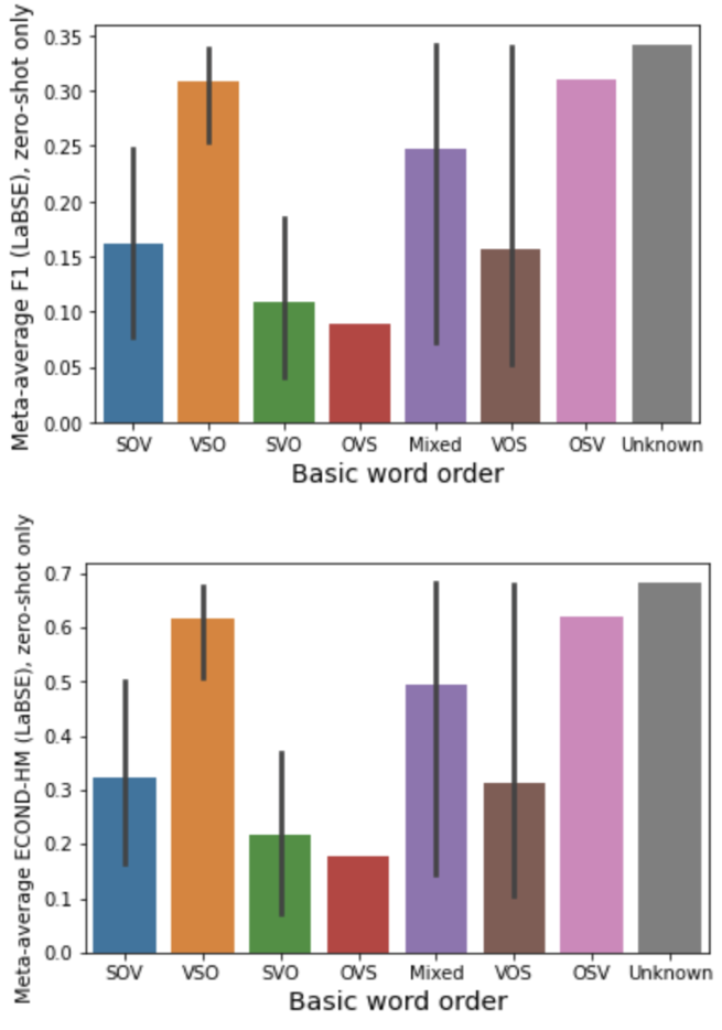
Figure 2: “Meta-average” performance of zero-shot languages with different word orders on F1-score and negative ECOND-HM (LaBSE).

Double Zero-shot Case

Interestingly, the language-pair-specific feature which stood out most in the double zero-shot case was inventory distance, an anomaly in our analyses. Inventory distance was correlated with $r\approx 0.2$-$0.4$ for 4/5 dependent variables for LaBSE and with $r\approx 0.13$-$0.14$ for 2/5 dependent variables for LASER.

However, as inventory distance quantifies phonological distance between languages, it could be confounded with surface-level information. To test this hypothesis, we regress it with character-level overlap and token-level overlap separately. For LaBSE, effects of inventory distance remain significant ($p<0.05$) for all dependent variables when regressing with token-level overlap, and 4/5 variables when regressing with character-level overlap. We wish to verify the importance of this feature in future studies.

8 Case Study 1: Morphological Segmentation of Inuktitut

Based on the above results, we conclude that whether a language has the same polysynthesis status as another language will affect their success on a cross-lingual task. However, our observations pertain to correlation, not causality. To test this observation further, we run an experiment in which we introduce a causal intervention. If indeed polysynthesis status matters, then we hypothesize that making a language “less polysynthetic” will improve alignment with a more analytic language like English.

To test this hypothesis, we examine the effect of morphological segmentation of Inuktitut on the bitext retrieval task. Inuktitut is a polysynthetic, indigenous language and is completely zero-shot for both our models, in that not even in-family data is provided during pretraining. The intuition behind our experiment is that by morphologically segmenting a polysynthetic language, the “polysynthesis status” of the segmented Inuktitut is made closer to that of a more analytic language. If our previous findings are correct, we expect Inuktitut to align better with English post-segmentation.

We use the first 10,000 sentences from the Nunavut Hansard Inuktitut-English parallel corpus Joanis et al. (2020) as our bitext. For the Inuktitut half of the corpus, we use both the “raw” version and a version that has been pre-segmented with the Uqailaut morphological analyzer.

We then perform bitext retrieval as described in section 4.1 on both bitexts: English aligned with non-segmented Inuktitut and English aligned with segmented Inuktitut. Results in terms of F1-score are displayed in Figure 3. For LaBSE, we see a $+$$28.7$ ($\approx 5\times$) F1-score increase using segmented Inuktitut; for LASER, we see a $+$$0.04$ ($1.5\times$) increase. These empirical results support our earlier statistical findings on the feature same polysynthesis status.

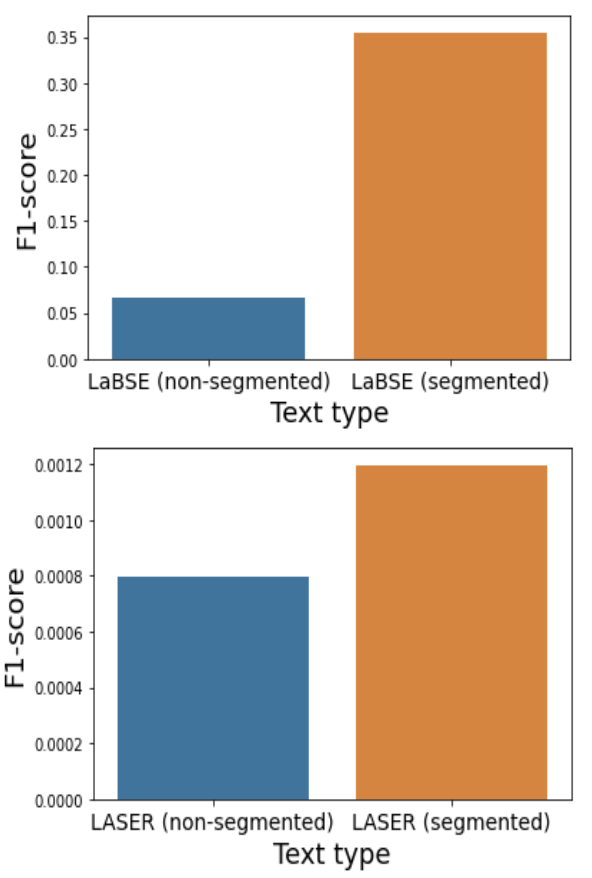
Figure 3: F1-scores on the bitext retrieval task for English-Inuktitut, using raw and morphologically segmented Inuktitut, for LaBSE (top) and LASER (bottom).

9 Case Study 2: Word Order & Isomorphism

To test the validity of our findings on the same word order feature, we examine whether embeddings in languages with similar word orders are more isomorphic to each other than those with substantially different word orders, sampling from a different corpus than the one we use in our main analysis. To this end, we select twelve zero-shot languages from the Universal Declaration of Human Rights (UDHR) parallel corpus Vatanen et al. (2010). Six of these are canonically verb-initial: K’iche’, Mam, Chinanteco, Tzotzil, Mixteco, and Garifuna. The other six are subject-initial: Chickasaw, Quechua, Achuar-Shiwiar, Bambara, Dagaare, and Guarani. We hypothesize that similar-word-order language pairs will be more isomorphic, on average, than pairs of languages with disparate word orders.

We compute SVG and ECOND-HM across all ${12\choose 2}=66$ language pairs for LaBSE and LASER separately and group the results based on whether the language pairs have similar word order or different word order. The averages of these groups are given in Table 4. Similar-word-order pairs are more isomorphic than their different-word-order counterparts across all metrics and both models.

	SVG	ECOND-HM
	LaBSE   LASER	LaBSE   LASER
Similar	5.63   3.67	18.08   18.13
Different	6.34   4.37	18.13   18.20

Table 4: Average values of SVG and ECOND-HM across 66 double zero-shot language pairs in the UDHR subset with similar or different word orders (based on whether a language is verb-initial or subject-initial). Note that LaBSE and LASER results are not comparable in absolute terms.

10 Conclusions

We find evidence that linguistic and quasi-linguistic factors continue to play a role in determining the cross-linguality of a model even after training data is accounted for, and validate our findings with two case studies on extremely low-resource languages. Our analysis points to, among other things, the importance of word order agreement (similarly to Pires et al. 2019) and morphology agreement on building aligned and isomorphic cross-lingual subspaces. We also rigorously demonstrate the importance of in-family training data in building massively multilingual models, and show moderate effects of other typological measures on cross-linguality. In the future, we are confident that these insights can be used to improve the cross-linguality of shared embedding spaces, particularly for low-resource languages.

11 Acknowledgements

We would like to thank Michael Saxon at the University of California, Santa Barbara for his suggestions regarding methodology; Ivan Vulić at the University of Cambridge for his advice on structuring our analysis; and Fangxiaoyu Feng at Google for providing training data statistics on LaBSE.

This work is partly sponsored by the Office of the Director of National Intelligence/Intelligence Advanced Research Projects Activity (IARPA). The views and conclusions contained in this document are those of the authors and should not be interpreted as representing the official policies, either expressed or implied, of the U.S. Government. The U.S. Government is authorized to reproduce and distribute reprints for Government purposes notwithstanding any copyright notation herein.

12 Ethical Considerations

When drawing inferences about multilingual language models, it is crucial to take into account languages that are low-resource, Indigenous, and endangered. Previous works have looked at the challenges facing these sorts of under-resourced and under-studied languages (e.g. Mager et al. 2018; Joshi et al. 2020) and proposed broad solutions and guidelines (e.g. Kann et al. 2019; Bender 2019).

The Bible corpus (Christodouloupoulos and Steedman, 2014) that we use in our analysis includes 35 languages that are zero-shot for LaBSE and 45 that are zero-shot for LASER, all of which could be classified as low-resource or extremely low-resource. This means that, for our case studies, we can test our conclusions on extremely low-resource languages (including Indigenous languages) that are typically underrepresented in NLP.

While the Bible corpus enables us to extend our work to low-resource languages, we also acknowledge that the corpus owes its existence largely to a settler colonial tradition, in which missionaries translated the Bible into Indigenous languages—often without crediting the Indigenous peoples who contributed their knowledge. We acknowledge these Indigenous peoples’ contributions to this work.

Studies such as Strubell et al. (2019) and Schwartz et al. (2019) have identified, analyzed, and proposed solutions for the energy consumption, cost, and environmental impact of NLP models, in particular the burdens associated with training and performing inference with large pretrained language models. Though we perform inference with two such models on a considerable amount of input, we note that these are one-time computations, made using a single NVIDIA V100 GPU, and that we plan to release our collected data publicly for reuse in future empirical analyses.

Appendix A Appendix

A.1 Issues With Using The Bible as a Corpus

We take note of several issues with using the Bible to perform cross-lingual analyses, but defend our decision to use it over other available corpora. The primary concern is with the language itself of the Bible and its translations: Much of it is archaic and would sound unnatural to modern speakers, and certain translations may suffer from sub-optimal (possibly non-native) translation quality. Furthermore, the relative performance of LaBSE and LASER on these texts was somewhat unrepresentative: LaBSE vastly outperformed LASER, despite the fact that they are closer in performance on more modern, idiomatic texts (e.g. the Tatoeba dataset from Artetxe and Schwenk (2019b)).

However, the Bible corpus from Christodouloupoulos and Steedman (2014) lends itself to our analysis in the following ways:

• Reliable sentence-level (technically verse-level) alignments

• Clean, easy-to-parse text

• Large-scale multilinguality and linguistic diversity

We also consider using JW300 Agić and Vulić (2019), the Tatoeba Challenge test data Tiedemann (2020), and the Johns Hopkins University Bible corpus McCarthy et al. (2020). However:

• JW300 is difficult to download in its entirety and sentence-align into a superparallel corpus in practice, and alignments may not be as clean as in the Bible corpus

• The Tatoeba Challenge bitexts are not multiparallel, so are useless for our main analysis

• The Johns Hopkins Bible corpus, while impressive in size with 1600+ languages, is overkill for the intended scale of our analysis (and, in practice, the quality of a corpus of this size is difficult to ascertain)

For these reasons, we viewed using the corpus from Christodouloupoulos and Steedman (2014) as a “necessary evil” of sorts to achieve the scale of analysis we were hoping for.

A.2 Choice of Embedding Models

We opt to use LaBSE (Feng et al., 2020) and LASER (Artetxe and Schwenk, 2019b) as our embedding models primarily because they are state-of-the-art sentence encoders that perform well on the bitext mining task (Reimers and Gurevych, 2020). Using two models with different underlying architectures (Transformer for LaBSE vs BiLSTM for LASER) makes our analysis more robust and generalizable, because any trend observed w.r.t. both models cannot be due to a peculiarity of one model or the other (e.g. training data domain, neural architecture, tokenization technique, etc.).

However, while both models have generally high performance on this task, LaBSE is, on average, superior to LASER (see Reimers and Gurevych (2020), but also our full results from this paper). On the lowest-resource languages and language pairs, we see an induced floor effect for LASER, where the variance among data points is low and statistical effects are hard to detect. For the same reason, we do not include results from mean-pooled subword embeddings—such as mBERT or XLM-RoBERTa—due to their relatively weak performance on the bitext mining task (Reimers and Gurevych, 2020).

Floor effects do not pose nearly as much of a problem for LaBSE. Thus, by including LaBSE as one of our models, we are able to detect fine-grained differences among low-resource languages and language pairs that we might miss with LASER. For higher-resource cases, our conclusions are made all the more robust for having inferences from two high-performing models.

A.3 Principal Component Analysis

We also perform principal component analysis (PCA) to determine how many independent components exist in our feature space, and how the loadings of those components break down.

A.3.1 Principal Component Regression

We run principal component regression (PCR) to determine the optimal number of components in our feature space for predicting the dependent variables. To this end, we first perform PCA on the full set of 13 features (separately for LaBSE and LASER, as the training features are different for each). We then perform PCR (with linear regression) using the first 1 to 13 components in separate runs, with each of the dependent variables being modeled separately as the regressand. As we did before, we measure regression fit using adjusted $r^{2}$ and average the results from ten-fold cross validation on each run.

We find that for LaBSE, the optimal number of components for predicting the dependent variables averaged 7.2, or roughly half the size of the feature space. For LASER, the average number of optimal components was 6.0.

A.3.2 Component Loadings

We also look at how the loadings of the principal components for LaBSE and LASER features break down; the results for the first five components are given in Table 5. For both LaBSE and LASER, the first three components map almost entirely onto training features, while later components are a mixture of the remaining features. However, same word order and same polysynthesis status are next after training-related features in terms of weight: they are the top two features in components 4 and 5 for both systems.

A.4 Semi-partial Correlations for Typological Distance

For the typological distance features, we use the semi-partial correlation Abdi (2007)

$$r_{1(2.3)}=\frac{r_{12}-r_{13}r_{23}}{\sqrt{1-r_{23}^{2}}}$$

where $r_{1(2.3)}$ is the correlation between $f_{1}$ and $f_{2}$ such that $f_{3}$ is held constant for $f_{2}$ (in our case, training data features are held constant for the dependent variables). This informs us how the typological distance features correlate with the dependent variables when training data features are modeled as covariates. We compute semi-partial correlations between each typological distance measure and each dependent variable for LaBSE and LASER separately.

The typological distance features had noteworthy ($r>0.1$) correlations for anywhere from 0/10 (phonological distance) to 5/10 (geographic distance) analyses. However, the $r$ values generally fell into the range $0.1<|r|<0.25$. We conclude that lang2vec distances correlate with cross-linguality weakly but non-negligibly when training data is held constant, somewhat contrary to the stronger relationships observed in Dubossarsky et al. (2020) with monolingual embedding spaces.

A.5 Visualization from Case Study 2

We visualize approximate isomorphism between select similar-word-order language pairs from section 9 with t-SNE van der Maaten and Hinton (2008), with default settings in scikit-learn. Results are displayed in Figure 4.

A.6 ECOND-HM Computation

The condition number of a matrix $\mathcal{X}$ with $n$ singular values $\sigma_{1},\sigma_{2},...,\sigma_{n}$, sorted in descending order, is defined as:

$$\kappa(\mathcal{X})=\frac{\sigma_{1}}{\sigma_{n}}$$

Furthermore, the effective rank of $\mathcal{X}$ is defined as:

$$\mathrm{rank}^{*}=\lfloor e^{H(\Sigma)}\rfloor$$

where $\lfloor\cdot\rfloor$ is the floor function and $H(\Sigma)$ is the entropy of the normalized singular value distribution of $\mathcal{X}$, namely $H(\Sigma)=-\sum_{i=1}^{n}{\bar{\sigma_{i}}\log{\bar{\sigma_{i}}}}$, where $\bar{\sigma_{i}}=\frac{\sigma_{i}}{\sum_{j=1}^{n}{\sigma_{j}}}$. Putting the two together, we define the effective condition number of $\mathcal{X}$ as:

$$\kappa_{eff}=\frac{\sigma_{1}}{\sigma_{\mathrm{rank}^{*}(\mathcal{X})}}$$

Finally, we define the effective condition number harmonic mean Dubossarsky et al. (2020) as:

$$\mathrm{ECOND\_HM}(\mathcal{X},\mathcal{Y})=\frac{2\cdot\kappa_{eff}(\mathcal{X})\cdot\kappa_{eff}({\mathcal{Y})}}{\kappa_{eff}(\mathcal{X})+\kappa_{eff}(\mathcal{Y})}$$

Using the effective rank instead of the standard rank to determine the (effective) condition number is a heuristic method motivated by finding the least singular value that characterizes $\mathcal{X}$ in a significant way, as informed by the entropy associated with the singular value distribution of $\mathcal{X}$.

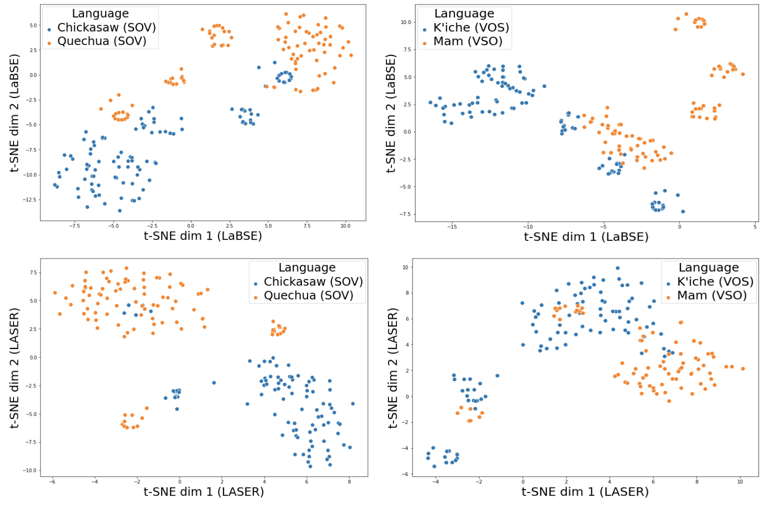
Figure 4: The first two t-SNE dimensions of sentence embeddings in the Universal Declaration of Human Rights, in four zero-shot languages (Chickasaw, Quechua, K’iche, and Mam). Languages with similar word order have been plotted together to demonstrate isomorphism of the resulting vector subspaces (LaBSE plots are top, LASER plots are bottom).

Feature	Loadings
	PC1	PC2	PC3	PC4	PC5
Combined sentences	2.50e-2, 5.28e-2	-2.30e-1, 2.53e-1	9.73e-1, 9.66e-1	-8.59e-11, -7.83e-10	1.12e-11, -5.93e-10
Combined in-family sentences	9.78e-1, 9.60e-1	2.07e-1, -2.81e-1	2.38e-2, 2.13e-2	-2.11e-11, -8.33-10	2.83e-12, -5.56e-12
Combined in-subfamily sentences	2.07e-1, 2.77e-1	-9.51e-1, 9.26e-1	-2.30e-1, -2.58e-1	-5.92e-12, 4.33e-10	1.15e-11, 4.40e-10
Same word order	1.10e-11, 3.42e-10	-5.38e-12, -4.97e-10	7.59e-11, 1.15e-9	7.60e-1, 7.13e-1	6.17e-1, 6.73e-1
Same polysynthesis status	1.57e-11, 4.30e-10	-2.21e-11, -8.02e-11	6.69e-11, 1.11e-10	6.02e-1, 6.54e-1	-7.81e-1, -7.33e-1
Same family	2.44e-11, 6.97e-10	-1.19e-12, -1.28e-10	-2.56e-11, -4.76e-11	1.67e-1, 1.84e-1	-6.07e-4, -1.11e-2
Same subfamily	3.64e-12, 1.10e-10	-1.48e-11, 1.19e-10	-1.81e-11, -7.06e-11	7.38e-2, 7.71e-2	1.45e-2, 1.65e-2
Token overlap	6.68e-12, 2.07e-10	-1.42e-11, 2.67e-11	-1.20e-11, 6.42e-12	6.23e-2, 6.48e-2	-1.87e-2, -1.77e-2
Character overlap	2.53e-12, 1.72e-10	-2.34e-11, 3.68e-10	-1.02e-10, -8.57e-11	4.93e-2, 2.39e-2	2.71e-2, 3.63e-2
Geographic distance	-4.28e-12, -1.29e-10	6.74e-13, 4.58e-11	-7.91e-13, -5.54e-11	-6.41e-2, -6.77e-2	6.45e-2, 6.20e-2
Syntactic distance	-7.48e-12, -2.36e-10	6.14e-12, 1.02e-10	1.53e-11, -2.23e-11	-9.85e-2, -9.33e-2	-6.25e-2, -6.48e-2
Phonological distance	-5.80e-12, -1.70e-10	-3.28e-12, 1.49e-10	2.87e-11, -9.04e-12	-5.81e-2, -5.71e-2	2.20e-2, 2.19e-2
Inventory distance	-8.39e-13, -2.12e-11	-3.53e-12, 1.05e-10	1.64e-11, -3.90e-11	-4.75e-2, -4.51e-2	1.49e-2 1.23e-2

Table 5: Loadings from the first five principal components for the language-pair-related features. The top three loadings by magnitude in each component are colored red for LaBSE and green for LASER. Note that although LaBSE and LASER are trained using different neural architectures, the most significant features in each of the first five components are almost identical.

References

- Abdi (2007) Hervé Abdi. 2007. Part (semi-partial) and Partial Regression Coefficients. Encyclopedia of measurement and statistics, pages 736–740.
- Achen (2005) Christopher H. Achen. 2005. Let’s Put Garbage-Can Regressions and Garbage-Can Probits Where They Belong. Conflict Management and Peace Science, 22(4):327–339.
- Agić and Vulić (2019) Željko Agić and Ivan Vulić. 2019. JW300: A wide-coverage parallel corpus for low-resource languages. In Proceedings of the 57th Annual Meeting of the Association for Computational Linguistics, pages 3204–3210, Florence, Italy. Association for Computational Linguistics.
- Artetxe and Schwenk (2019a) Mikel Artetxe and Holger Schwenk. 2019a. Margin-based parallel corpus mining with multilingual sentence embeddings. In Proceedings of the 57th Annual Meeting of the Association for Computational Linguistics, pages 3197–3203, Florence, Italy. Association for Computational Linguistics.
- Artetxe and Schwenk (2019b) Mikel Artetxe and Holger Schwenk. 2019b. Massively multilingual sentence embeddings for zero-shot cross-lingual transfer and beyond. Transactions of the Association for Computational Linguistics, 7:597–610.
- Bender (2019) Emily Bender. 2019. The #BenderRule: On Naming the Languages We Study and Why It Matters. The Gradient.
- Bojanowski et al. (2016) Piotr Bojanowski, Edouard Grave, Armand Joulin, and Tomas Mikolov. 2016. Enriching Word Vectors with Subword Information. arXiv e-prints, page arXiv:1607.04606.
- Chazal et al. (2009) Frédéric Chazal, David Cohen-Steiner, Leonidas J. Guibas, Facundo Mémoli, and Steve Y. Oudot. 2009. Gromov-Hausdorff Stable Signatures for Shapes using Persistence. Computer Graphics Forum, 28(5):1393–1403.
- Christodouloupoulos and Steedman (2014) Christos Christodouloupoulos and Mark Steedman. 2014. A Massively Parallel Corpus: the Bible in 100 Languages. Language Resources and Evaluation, 49(2):375–395.
- Cohen (1988) Jacob Cohen. 1988. Statistical Power Analysis for the Behavioral Sciences, 2 edition. L. Erlbaum Associates.
- Conneau et al. (2020) Alexis Conneau, Shijie Wu, Haoran Li, Luke Zettlemoyer, and Veselin Stoyanov. 2020. Emerging cross-lingual structure in pretrained language models. In Proceedings of the 58th Annual Meeting of the Association for Computational Linguistics, pages 6022–6034, Online. Association for Computational Linguistics.
- Cotterell et al. (2019) Ryan Cotterell, Christo Kirov, Mans Hulden, and Jason Eisner. 2019. On the complexity and typology of inflectional morphological systems. Transactions of the Association for Computational Linguistics, 7:327–342.
- Dror et al. (2018) Rotem Dror, Gili Baumer, Segev Shlomov, and Roi Reichart. 2018. The hitchhiker’s guide to testing statistical significance in natural language processing. In Proceedings of the 56th Annual Meeting of the Association for Computational Linguistics (Volume 1: Long Papers), pages 1383–1392, Melbourne, Australia. Association for Computational Linguistics.
- Dryer and Haspelmath (2013) Matthew S. Dryer and Martin Haspelmath, editors. 2013. WALS Online. Max Planck Institute for Evolutionary Anthropology, Leipzig.
- Dubossarsky et al. (2020) Haim Dubossarsky, Ivan Vulić, Roi Reichart, and Anna Korhonen. 2020. The secret is in the spectra: Predicting cross-lingual task performance with spectral similarity measures. In Proceedings of the 2020 Conference on Empirical Methods in Natural Language Processing (EMNLP), pages 2377–2390, Online. Association for Computational Linguistics.
- Fan et al. (2020) Angela Fan, Shruti Bhosale, Holger Schwenk, Zhiyi Ma, Ahmed El-Kishky, Siddharth Goyal, Mandeep Baines, Onur Celebi, Guillaume Wenzek, Vishrav Chaudhary, Naman Goyal, Tom Birch, Vitaliy Liptchinsky, Sergey Edunov, Edouard Grave, Michael Auli, and Armand Joulin. 2020. Beyond English-Centric Multilingual Machine Translation. arXiv e-prints, page arXiv:2010.11125.
- Feng et al. (2020) Fangxiaoyu Feng, Yinfei Yang, Daniel Cer, Naveen Arivazhagan, and Wei Wang. 2020. Language-agnostic BERT Sentence Embedding. arXiv e-prints, page arXiv:2007.01852.
- Groenwold et al. (2020) Sophie Groenwold, Samhita Honnavalli, Lily Ou, Aesha Parekh, Sharon Levy, Diba Mirza, and William Yang Wang. 2020. Evaluating Transformer-Based Multilingual Text Classification. arXiv e-prints, page arXiv:2004.13939.
- Hammarström et al. (2020) Harald Hammarström, Robert Forkel, Martin Haspelmath, and Sebastian Bank. 2020. Glottolog Database 4.3.
- Joanis et al. (2020) Eric Joanis, Rebecca Knowles, Roland Kuhn, Samuel Larkin, Patrick Littell, Chi-kiu Lo, Darlene Stewart, and Jeffrey Micher. 2020. The Nunavut hansard Inuktitut–English parallel corpus 3.0 with preliminary machine translation results. In Proceedings of the 12th Language Resources and Evaluation Conference, pages 2562–2572, Marseille, France. European Language Resources Association.
- Johnson et al. (2017a) Jeff Johnson, Matthijs Douze, and Hervé Jégou. 2017a. Billion-scale Similarity Search with GPUs. arXiv preprint arXiv:1702.08734.
- Johnson et al. (2017b) Melvin Johnson, Mike Schuster, Quoc V. Le, Maxim Krikun, Yonghui Wu, Zhifeng Chen, Nikhil Thorat, Fernanda Viégas, Martin Wattenberg, Greg Corrado, Macduff Hughes, and Jeffrey Dean. 2017b. Google’s multilingual neural machine translation system: Enabling zero-shot translation. Transactions of the Association for Computational Linguistics, 5:339–351.
- Jones and Wijaya (2021) Alex Jones and Derry Wijaya. 2021. Majority Voting with Bidirectional Pre-translation For Bitext Retrieval. arXiv e-prints, page arXiv:2103.06369.
- Joshi et al. (2020) Pratik Joshi, Sebastin Santy, Amar Budhiraja, Kalika Bali, and Monojit Choudhury. 2020. The state and fate of linguistic diversity and inclusion in the NLP world. In Proceedings of the 58th Annual Meeting of the Association for Computational Linguistics, pages 6282–6293, Online. Association for Computational Linguistics.
- Joulin et al. (2016) Armand Joulin, Edouard Grave, Piotr Bojanowski, and Tomas Mikolov. 2016. Bag of Tricks for Efficient Text Classification. arXiv e-prints, page arXiv:1607.01759.
- Kann et al. (2019) Katharina Kann, Kyunghyun Cho, and Samuel R. Bowman. 2019. Towards realistic practices in low-resource natural language processing: The development set. In Proceedings of the 2019 Conference on Empirical Methods in Natural Language Processing and the 9th International Joint Conference on Natural Language Processing (EMNLP-IJCNLP), pages 3342–3349, Hong Kong, China. Association for Computational Linguistics.
- Karthikeyan et al. (2020) K Karthikeyan, Zihan Wang, Stephen Mayhew, and Dan Roth. 2020. Cross-lingual ability of multilingual bert: An empirical study. In International Conference on Learning Representations.
- Keung et al. (2021) Phillip Keung, Julian Salazar, Yichao Lu, and Noah A. Smith. 2021. Unsupervised Bitext Mining and Translation via Self-Trained Contextual Embeddings. Transactions of the Association for Computational Linguistics, 8:828–841.
- Lin et al. (2019) Yu-Hsiang Lin, Chian-Yu Chen, Jean Lee, Zirui Li, Yuyan Zhang, Mengzhou Xia, Shruti Rijhwani, Junxian He, Zhisong Zhang, Xuezhe Ma, Antonios Anastasopoulos, Patrick Littell, and Graham Neubig. 2019. Choosing transfer languages for cross-lingual learning. In Proceedings of the 57th Annual Meeting of the Association for Computational Linguistics, pages 3125–3135, Florence, Italy. Association for Computational Linguistics.
- Littell et al. (2019) Patrick Littell, Chi-kiu Lo, Samuel Larkin, and Darlene Stewart. 2019. Multi-source transformer for Kazakh-Russian-English neural machine translation. In Proceedings of the Fourth Conference on Machine Translation (Volume 2: Shared Task Papers, Day 1), pages 267–274, Florence, Italy. Association for Computational Linguistics.
- Littell et al. (2017) Patrick Littell, David R. Mortensen, Ke Lin, Katherine Kairis, Carlisle Turner, and Lori Levin. 2017. URIEL and lang2vec: Representing languages as typological, geographical, and phylogenetic vectors. In Proceedings of the 15th Conference of the European Chapter of the Association for Computational Linguistics: Volume 2, Short Papers, pages 8–14, Valencia, Spain. Association for Computational Linguistics.
- Mager et al. (2018) Manuel Mager, Ximena Gutierrez-Vasques, Gerardo Sierra, and Ivan Meza-Ruiz. 2018. Challenges of language technologies for the indigenous languages of the Americas. In Proceedings of the 27th International Conference on Computational Linguistics, pages 55–69, Santa Fe, New Mexico, USA. Association for Computational Linguistics.
- Malaviya et al. (2017) Chaitanya Malaviya, Graham Neubig, and Patrick Littell. 2017. Learning language representations for typology prediction. In Proceedings of the 2017 Conference on Empirical Methods in Natural Language Processing, pages 2529–2535, Copenhagen, Denmark. Association for Computational Linguistics.
- McCarthy et al. (2020) Arya D. McCarthy, Rachel Wicks, Dylan Lewis, Aaron Mueller, Winston Wu, Oliver Adams, Garrett Nicolai, Matt Post, and David Yarowsky. 2020. The Johns Hopkins University Bible corpus: 1600+ tongues for typological exploration. In Proceedings of the 12th Language Resources and Evaluation Conference, pages 2884–2892, Marseille, France. European Language Resources Association.
- Mikolov et al. (2013) Tomas Mikolov, Kai Chen, Greg Corrado, and Jeffrey Dean. 2013. Efficient Estimation of Word Representations in Vector Space. arXiv e-prints, page arXiv:1301.3781.
- Pires et al. (2019) Telmo Pires, Eva Schlinger, and Dan Garrette. 2019. How multilingual is multilingual BERT? In Proceedings of the 57th Annual Meeting of the Association for Computational Linguistics, pages 4996–5001, Florence, Italy. Association for Computational Linguistics.
- Reimers and Gurevych (2020) Nils Reimers and Iryna Gurevych. 2020. Making monolingual sentence embeddings multilingual using knowledge distillation. In Proceedings of the 2020 Conference on Empirical Methods in Natural Language Processing (EMNLP), pages 4512–4525, Online. Association for Computational Linguistics.
- Rogers et al. (2020) Anna Rogers, Olga Kovaleva, and Anna Rumshisky. 2020. A primer in BERTology: What we know about how BERT works. Transactions of the Association for Computational Linguistics, 8:842–866.
- Salkind (2017) Neil J. Salkind. 2017. Post Hoc Tests: Tukey Honestly Significant Difference Test. The SAGE Encyclopedia of Communication Research Methods.
- Schwartz et al. (2019) Roy Schwartz, Jesse Dodge, Noah A. Smith, and Oren Etzioni. 2019. Green AI. arXiv e-prints, page arXiv:1907.10597.
- Schwenk et al. (2021) Holger Schwenk, Vishrav Chaudhary, Shuo Sun, Hongyu Gong, and Francisco Guzmán. 2021. WikiMatrix: Mining 135M parallel sentences in 1620 language pairs from Wikipedia. In Proceedings of the 16th Conference of the European Chapter of the Association for Computational Linguistics: Main Volume, pages 1351–1361, Online. Association for Computational Linguistics.
- Schwenk et al. (2019) Holger Schwenk, Guillaume Wenzek, Sergey Edunov, Edouard Grave, and Armand Joulin. 2019. CCMatrix: Mining Billions of High-Quality Parallel Sentences on the WEB. arXiv e-prints, page arXiv:1911.04944.
- Strubell et al. (2019) Emma Strubell, Ananya Ganesh, and Andrew McCallum. 2019. Energy and policy considerations for deep learning in NLP. In Proceedings of the 57th Annual Meeting of the Association for Computational Linguistics, pages 3645–3650, Florence, Italy. Association for Computational Linguistics.
- Tiedemann (2020) Jörg Tiedemann. 2020. The tatoeba translation challenge – realistic data sets for low resource and multilingual MT. In Proceedings of the Fifth Conference on Machine Translation, pages 1174–1182, Online. Association for Computational Linguistics.
- Tran et al. (2020) Chau Tran, Yuqing Tang, Xian Li, and Jiatao Gu. 2020. Cross-lingual Retrieval for Iterative Self-supervised Training. arXiv preprint arXiv:2006.09526.
- van der Maaten and Hinton (2008) Laurens van der Maaten and Geoffrey Hinton. 2008. Visualizing Data using t-SNE. Journal of Machine Learning Research, 9(86):2579–2605.
- Vatanen et al. (2010) Tommi Vatanen, Jaakko J. Väyrynen, and Sami Virpioja. 2010. Language identification of short text segments with n-gram models. In Proceedings of the Seventh International Conference on Language Resources and Evaluation (LREC’10), Valletta, Malta. European Language Resources Association (ELRA).
- Vulić et al. (2020) Ivan Vulić, Sebastian Ruder, and Anders Søgaard. 2020. Are all good word vector spaces isomorphic? In Proceedings of the 2020 Conference on Empirical Methods in Natural Language Processing (EMNLP), pages 3178–3192, Online. Association for Computational Linguistics.
- Wolf et al. (2020) Thomas Wolf, Lysandre Debut, Victor Sanh, Julien Chaumond, Clement Delangue, Anthony Moi, Pierric Cistac, Tim Rault, Remi Louf, Morgan Funtowicz, Joe Davison, Sam Shleifer, Patrick von Platen, Clara Ma, Yacine Jernite, Julien Plu, Canwen Xu, Teven Le Scao, Sylvain Gugger, Mariama Drame, Quentin Lhoest, and Alexander Rush. 2020. Transformers: State-of-the-art natural language processing. In Proceedings of the 2020 Conference on Empirical Methods in Natural Language Processing: System Demonstrations, pages 38–45, Online. Association for Computational Linguistics.
- Wu and Dredze (2019) Shijie Wu and Mark Dredze. 2019. Beto, bentz, becas: The surprising cross-lingual effectiveness of BERT. In Proceedings of the 2019 Conference on Empirical Methods in Natural Language Processing and the 9th International Joint Conference on Natural Language Processing (EMNLP-IJCNLP), pages 833–844, Hong Kong, China. Association for Computational Linguistics.
- Wu and Dredze (2020) Shijie Wu and Mark Dredze. 2020. Are all languages created equal in multilingual BERT? In Proceedings of the 5th Workshop on Representation Learning for NLP, pages 120–130, Online. Association for Computational Linguistics.
- Wu et al. (2016) Yonghui Wu, Mike Schuster, Zhifeng Chen, Quoc V. Le, Mohammad Norouzi, Wolfgang Macherey, Maxim Krikun, Yuan Cao, Qin Gao, Klaus Macherey, Jeff Klingner, Apurva Shah, Melvin Johnson, Xiaobing Liu, Łukasz Kaiser, Stephan Gouws, Yoshikiyo Kato, Taku Kudo, Hideto Kazawa, Keith Stevens, George Kurian, Nishant Patil, Wei Wang, Cliff Young, Jason Smith, Jason Riesa, Alex Rudnick, Oriol Vinyals, Greg Corrado, Macduff Hughes, and Jeffrey Dean. 2016. Google’s Neural Machine Translation System: Bridging the Gap between Human and Machine Translation. CoRR, abs/1609.08144.
- Xia et al. (2021) Mengzhou Xia, Guoqing Zheng, Subhabrata Mukherjee, Milad Shokouhi, Graham Neubig, and Ahmed Hassan Awadallah. 2021. MetaXL: Meta Representation Transformation for Low-resource Cross-lingual Learning. arXiv e-prints, page arXiv:2104.07908.
- Zhang et al. (2019) Mozhi Zhang, Keyulu Xu, Ken-ichi Kawarabayashi, Stefanie Jegelka, and Jordan Boyd-Graber. 2019. Are girls neko or shōjo? cross-lingual alignment of non-isomorphic embeddings with iterative normalization. In Proceedings of the 57th Annual Meeting of the Association for Computational Linguistics, pages 3180–3189, Florence, Italy. Association for Computational Linguistics.