Stochastic Observer for SLAM on the Lie Group

Abstract

A robust nonlinear stochastic observer for simultaneous localization and mapping (SLAM) is proposed using the available uncertain measurements of angular velocity, translational velocity, and features. The proposed observer is posed on the Lie Group of $\mathbb{SLAM}_{n}\left(3\right)$ to mimic the true stochastic SLAM dynamics. The proposed approach considers the velocity measurements to be attached with an unknown bias and an unknown Gaussian noise. The proposed SLAM observer ensures that the closed loop error signals are semi-globally uniformly ultimately bounded. Simulation results demonstrates the efficiency and robustness of the proposed approach, revealing its ability to localize the unknown vehicle, as well as mapping the unknown environment given measurements obtained from low-cost units.

I Introduction

Navigation is an essential part of robotics and control applications [1, 2]. Successful navigation of a vehicle in three dimensional (3D) space requires an accurate estimation of its pose (i.e., attitude and position) as well as a map of the environment. The estimation of a vehicle’s pose and mapping of the environment is known as simultaneous localization and mapping (SLAM). SLAM related applications are indispensable in indoor and outdoor applications, especially in harsh environments. Over the last twenty years, SLAM estimation has been studied extensively [3, 4, 5, 6, 7, 8, 9, 10, 11]. SLAM estimation is accomplished using a group of sensor measurements, where the sensors are attached to the body of the vehicle. The price of a vehicle drops significantly in case of using low-cost sensing units, but unfortunately, low-cost sensors are attached with high levels of uncertainties, which compromise the estimation process. Therefore, robust observers are necessary to compensate for the uncertainties and to produce a reasonable estimate of the vehicle’s pose, as well as features of the environment.

In the past, the SLAM estimation problem have been addressed using classical approaches that are commonly known as Gaussian filters [12]. Examples include; the monoSLAM with object recognition using real-time single camera [13], neuro-adaptive FastSLAM approach [14], incremental SLAM with constrained optimization [15], data fusion real-time RGB-D SLAM [16], compressed unscented Kalman filter [17], and others. However, the SLAM problem is composed of two main parts: the vehicle’s pose and the features. The true feature dynamics are modeled on the Lie Group of the Special Orthogonal Group $\mathbb{SO}\left(3\right)$, while the vehicle’s pose dynamics are modeled on the Lie Group of the Special Euclidean Group $\mathbb{SE}\left(3\right)=\mathbb{SO}\left(3\right)\times\mathbb{R}^{3}$ [12, 18]. Hence, the true SLAM problem is highly nonlinear posed on the Lie Group $\mathbb{SLAM}_{n}\left(3\right)=\mathbb{SE}\left(3\right)\times\mathbb{R}^{3}\times\cdots\times\mathbb{R}^{3}$ which is not the unique source of complexity. Therefore, the SLAM problem is better addressed on the Lie Group of $\mathbb{SLAM}_{n}\left(3\right)$ [7, 8]. Over the last few years, nonlinear filters for SLAM have increasingly become a perfect alternative to supplant Gaussian filters. Examples of such include nonlinear filters that rely on the measurements of angular velocity, translational velocity, and features [7, 8]. Other nonlinear filters have also been proposed rely on the previously mentioned measurements, as well as the inertial measurement unit (IMU) attached to the rigid-body of the vehicle [12, 18, 19, 5]. The solutions in [7, 8, 18, 12] are nonlinear deterministic filters that compensate for unknown constant bias attached to velocity measurements while the solution in [5] is a nonlinear stochastic filter compensates not only for the unknown constant bias but also for random noise. It’s worth noting that the transient and steady-state error performance can be controlled using the techniques in [7, 18]. To conclude, despite the fact that the SLAM has been addressed in a stochastic sense, using stochastic differential equation in [5], the proposed algorithm relies on IMU data. This requirement increases the computational cost.

In the present paper the SLAM problem is addressed on stochastic sense on the Lie Group of $\mathbb{SLAM}_{n}\left(3\right)$, similar to [5]. Hence, the velocity data are assumed to be corrupted with an unknown, constant bias and a Gaussian random noise. Unlike [5], a nonlinear stochastic observer for SLAM is proposed, capable of functioning without the need for IMU data. The closed loop error signals are ensured to be semi-globally uniformly ultimately bounded.

After the above, the remainder of the paper is composed of four Sections. Section II presents the preliminaries of $\mathbb{SO}\left(3\right)$ and $\mathbb{SE}\left(3\right)$, the true SLAM dynamics and measurements, and error criteria. In Section II a nonlinear stochastic estimator for SLAM is proposed , along with it’s stability analysis. In Section IV. the effectiveness of the proposed SLAM observer schemes is demonstrated. Finally, Section V presents the concluding results.

II Problem Formulation

Notation
$\mathbb{R}$	set of real numbers
$\mathbb{R}^{p\times q}$	real space of dimension $p$-by-$q$
$\mathbf{I}_{n}\in\mathbb{R}^{n\times n}$	identity matrix
$\left\|\cdot\right\|$	Euclidean norm of a vector
$\mathbb{SO}\left(3\right)$	Special Orthogonal Group
$\mathbb{SE}\left(3\right)$	Special Euclidean Group

II-A Preliminaries

The attitude of a vehicle is defined by $R\in\mathbb{SO}\left(3\right)$ where $\mathbb{SO}\left(3\right)$ denotes the Special Orthogonal Group

$$\mathbb{SO}\left(3\right)=\left\{\left.R\in\mathbb{R}^{3\times 3}\right|RR^{\top}=\mathbf{I}_{3}\text{, }{\rm det}\left(R\right)=+1\right\}$$

$\left[\cdot\right]_{\times}$ denotes skew symmetric of a component such that for $n\in\mathbb{R}^{3}$, one has:

$$\left[n\right]_{\times}=\left[\begin{array}[]{ccc}0&-n_{3}&n_{2}\\ n_{3}&0&-n_{1}\\ -n_{2}&n_{1}&0\end{array}\right]\in\mathfrak{so}\left(3\right),\hskip 10.00002ptn=\left[\begin{array}[]{c}n_{1}\\ n_{2}\\ n_{3}\end{array}\right]$$

Pose of a vehicle can be represented by

$$\boldsymbol{T}=\left[\begin{array}[]{cc}R&P\\ 0_{1\times 3}&1\end{array}\right]\in\mathbb{SE}\left(3\right)\subset\mathbb{R}^{4\times 4}$$ (1)

where $R\in\mathbb{SO}\left(3\right)$ denotes the vehicle’s attitude, $P\in\mathbb{R}^{3}$ denotes vehicle’s position, $\boldsymbol{T}$ denotes the homogeneous transformation matrix, and $\mathbb{SE}\left(3\right)$ is the Special Euclidean Group given by

$$\mathbb{SE}\left(3\right)=\left\{\left.\boldsymbol{T}=\left[\begin{array}[]{cc}R&P\\ 0_{1\times 3}&1\end{array}\right]\right|R\in\mathbb{SO}\left(3\right),P\in\mathbb{R}^{3}\right\}$$

II-B Dynamics and Measurements

The SLAM problem considers a vehicle, whose pose is unknown, navigating in an unknown environment. The unknown environment can be defined through $n$ features. The vehicle’s pose is denoted by $\boldsymbol{T}\in\mathbb{SE}\left(3\right)$ and ${\rm p}_{i}\in\mathbb{R}^{3}$. Fig. 1 shows the SLAM estimation problem in a 3D space.

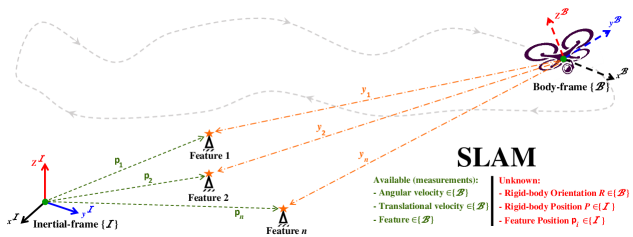
Figure 1: SLAM estimation problem [7].

The true dynamics of the vehicle’s pose and the $i$th feature can be described by [7]

$$\left[\begin{array}[]{cc}\dot{R}&\dot{P}\\ 0_{1\times 3}&0\end{array}\right] =\left[\begin{array}[]{cc}R&P\\ 0_{1\times 3}&1\end{array}\right]\left[\begin{array}[]{cc}\left[\Omega\right]_{\times}&V\\ 0_{1\times 3}&0\end{array}\right]$$ (8)

$$\dot{{\rm p}}_{i} =R{\rm v}_{i},\hskip 10.00002pt\forall i=1,2,\ldots,n$$ (9)

or to put simply

$$\begin{cases}\dot{R}&=R\left[\Omega\right]_{\times}\\ \dot{P}&=RV\\ \dot{{\rm p}}_{i}&=R{\rm v}_{i},\hskip 10.00002pt\forall i=1,2,\ldots,n\end{cases}$$

where $\Omega\in\mathbb{R}^{3}$ denotes the vehicle’s angular velocity, while $V\in\mathbb{R}^{3}$ denotes the vehicle’s translational velocity. It is worth noting that the SLAM dynamics in (8) and (9) are posed on the Lie Group of $\mathbb{SLAM}_{n}\left(3\right)$, see [7, 18]. Let $n$ features be available for measurement in the vehicle’s frame (body-frame), which can be obtained by a local vision unit. The $i$th measurement is described by [20]:

$$y_{i}=R^{\top}({\rm p}_{i}-P)+b_{i}^{y}+n_{i}^{y}\in\mathbb{R}^{3}$$ (10)

for $i=1,2,\ldots,n$.

Assumption 1

At least 3 measured, non-collinear features ($n=3$) define a plane that’s available at every time instant.

Angular velocity measurements are given by [21, 5, 22, 23]:

$$\Omega_{m}=\Omega+b_{\Omega}+n_{\Omega}\in\mathbb{R}^{3}$$ (11)

where $b_{\Omega}$ denotes a constant bias and $n_{\Omega}$ describes an unknown noise. Likewise, translational velocity measurement is described by [20]:

$$V_{m}=V+b_{V}+n_{V}\in\mathbb{R}^{3}$$ (12)

where $b_{V}$ denotes a constant bias and $n_{V}$ describes an unknown noise. Unknown uncertainties presenting challenge in variety of applications [5, 21, 24, 25].

II-C Dynamics in Stochastic Sense

Let $\left\{n_{\Omega},t\geq t_{0}\right\}$ and $\left\{n_{V},t\geq t_{0}\right\}$ be vector representations of independent, Brownian motion processes [26, 21, 27, 20]:

$$n_{\Omega}=\mathcal{Q}_{\Omega}\frac{d\beta_{\Omega}}{dt},\hskip 10.00002ptn_{V}=\mathcal{Q}_{V}\frac{d\beta_{V}}{dt}$$ (13)

where $\mathcal{Q}_{\Omega}\in\mathbb{R}^{3\times 3}$ and $\mathcal{Q}_{V}\in\mathbb{R}^{3\times 3}$ refer to an unknown nonzero non-negative diagonal matrix. Note that $\mathcal{Q}_{\Omega}$ and $\mathcal{Q}_{V}$ are bounded and time-variant. $\mathcal{Q}_{\Omega}^{2}=\mathcal{Q}_{\Omega}\mathcal{Q}_{\Omega}^{\top}$ and $\mathcal{Q}_{V}^{2}=\mathcal{Q}_{V}\mathcal{Q}_{V}^{\top}$ denote the covariance associated with the noises $n_{\Omega}$ and $n_{V}$, respectively. It is worth noting that $\mathbb{P}\left\{\beta_{\Omega}\left(0\right)=0\right\}=1,$ $\mathbb{P}\left\{\beta_{V}\left(0\right)=0\right\}=1,$ $\mathbb{E}\left[d\beta_{\Omega}/dt\right]=\mathbb{E}\left[\beta_{\Omega}\right]=0$, and $\mathbb{E}\left[d\beta_{V}/dt\right]=\mathbb{E}\left[\beta_{V}\right]=0$ such that $\mathbb{P}\left\{\cdot\right\}$ denotes the probability of an element while $\mathbb{E}[\cdot]$ refers to the expected value of an element [28]. Thus, the dynamics in (8) and (9) can be reformulated as:

$$dR =R[\Omega_{m}-b_{\Omega}]_{\times}dt-R\left[\mathcal{Q}_{\Omega}d\beta_{\Omega}\right]_{\times}$$ (14)

$$dP =R(V_{m}-b_{V})dt-R\mathcal{Q}_{V}d\beta_{V}$$ (15)

$$d{\rm p}_{i} =R{\rm v}_{i}dt,\hskip 10.00002pt\forall i=1,2,\ldots,n$$ (16)

Now, let us define $\sigma$ as:

$$\sigma=\left[\begin{array}[]{c}{\rm max}\left\{\mathcal{Q}_{\Omega\left(1,1\right)}^{2},\mathcal{Q}_{V\left(1,1\right)}^{2}\right\}\\ {\rm max}\left\{\mathcal{Q}_{\Omega\left(2,2\right)}^{2},\mathcal{Q}_{V\left(2,2\right)}^{2}\right\}\\ {\rm max}\left\{\mathcal{Q}_{\Omega\left(3,3\right)}^{2},\mathcal{Q}_{V\left(3,3\right)}^{2}\right\}\end{array}\right]$$ (17)

where ${\rm max}\left\{\cdot\right\}$ denotes the maximum value of the associated component.

III Stochastic Observer Design

The objective of this Section is to propose a stochastic observer on the Lie Group of $\mathbb{SLAM}_{n}\left(3\right)$, capable of localizing the unknown vehicle’s pose and map the unknown environment. First, define the estimate of attitude, position, and the $i$th feature as $\hat{R}$, $\hat{P}$, and $\hat{{\rm p}}_{i}$, respectively. Let the error in the vehicle’s pose be given as:

$$\hat{\boldsymbol{T}}\boldsymbol{T}^{-1} =\left[\begin{array}[]{cc}\hat{R}&\hat{P}\\ 0_{1\times 3}&1\end{array}\right]\left[\begin{array}[]{cc}R^{\top}&-R^{\top}P\\ 0_{1\times 3}&1\end{array}\right]$$ (22)

$$=\left[\begin{array}[]{cc}\tilde{R}&\tilde{P}\\ 0_{1\times 3}&1\end{array}\right]$$ (25)

where $\tilde{R}=\hat{R}R^{\top}$ and $\tilde{P}=\hat{P}-\tilde{R}P$. Then, let the error in the feature be defined as

$$\tilde{{\rm p}}_{i}=\hat{{\rm p}}_{i}-\tilde{R}{\rm p}_{i}$$ (26)

Let $\hat{b}_{\Omega}$ be the estimate of $b_{\Omega}$, $\hat{b}_{V}$ be the estimate of $b_{V}$, and $\hat{\sigma}$ be the estimate of $\sigma$. Define the error in bias as:

$$\tilde{b}_{\Omega} =b_{\Omega}-\hat{b}_{\Omega}$$

$$\tilde{b}_{V} =b_{V}-\hat{b}_{V}$$ (27)

Then define the error in the upper-bound covariance as

$$\tilde{\sigma}_{\Omega} =\sigma-\hat{\sigma}$$ (28)

And define the $i$th error component as

$$e_{i}=\hat{{\rm p}}_{i}-\hat{R}y_{i}-\hat{P}=\tilde{{\rm p}}_{i}-\tilde{P}$$ (29)

The stochastic error dynamics, which will be defined in the subsequent subsection are equivalent to:

$$de_{i}=f(e_{i},\tilde{b})dt+g(e_{i})\mathcal{Q}d\beta$$ (30)

where $\mathcal{Q}=\left[\begin{array}[]{cc}\mathcal{Q}_{\Omega}&0_{3\times 3}\\ 0_{3\times 3}&\mathcal{Q}_{V}\end{array}\right]\in\mathbb{R}^{6\times 6}$ and $\beta=[\beta_{\Omega}^{\top},\beta_{V}^{\top}]^{\top}\in\mathbb{R}^{6}$.

Definition 1

[28, 21] For the stochastic system in (30), Let $V(e_{i})$ be a twice differentiable cost function. The differential operator is as follows:

$$\mathcal{L}V\left(e_{i}\right)=V_{e_{i}}^{\top}f+\frac{1}{2}{\rm Tr}\left\{g\mathcal{Q}^{2}g^{\top}V_{e_{i}e_{i}}\right\}$$

with $V_{e_{i}}=\partial V/\partial e_{i}$ and $V_{e_{i}e_{i}}=\partial^{2}V/\partial e_{i}^{2}$.

Lemma 1

[27] For the stochastic dynamics in (30) let $V(e_{i})$ be a twice differentiable cost function. Define $\bar{\upsilon}_{1}(\cdot)$ and $\bar{\upsilon}_{2}(\cdot)$ as class $\mathcal{K}_{\infty}$ functions and define $\boldsymbol{{\rm c}}>0$ and $\mathbf{k}\geq 0$ as scalars. Let $\boldsymbol{\mathcal{N}}(||e_{i}||)$ be a non-negative function where,

$$\bar{\upsilon}_{1}(||e_{i}||)\leq V\leq\bar{\upsilon}_{2}(||e_{i}||)$$ (31)

$$\mathcal{L}V(e_{i})= V_{e_{i}}^{\top}f+\frac{1}{2}{\rm Tr}\left\{g\mathcal{Q}^{2}g^{\top}V_{e_{i}e_{i}}\right\}$$

$$\leq -\boldsymbol{{\rm c}}\boldsymbol{\mathcal{N}}(||e_{i}||)+\mathbf{k}$$ (32)

Then for $e_{i}(0)\in\mathbb{R}^{3}$, there is an almost unique strong solution on $\left[0,\infty\right)$ for (30). Also, $e_{i}$ is bounded in probability, following the inequality below:

$$\mathbb{E}\left[V\left(e_{i}\right)\right]\leq V\left(e_{i}\left(0\right)\right){\rm exp}\left(-\boldsymbol{{\rm c}}t\right)+\frac{\mathbf{k}}{\boldsymbol{{\rm c}}}$$ (33)

and $e_{i}$ is semi-globally uniformly ultimately bounded.

Consider the following nonlinear stochastic observer on the Lie Group of $\mathbb{SLAM}_{n}\left(3\right)$:

$$\dot{\hat{\boldsymbol{T}}}= \hat{\boldsymbol{T}}\left[\begin{array}[]{cc}\left[\Omega_{m}-\hat{b}_{\Omega}-W_{\Omega}\right]_{\times}&V_{m}-\hat{b}_{V}-W_{V}\\ 0_{1\times 3}&0\end{array}\right]$$ (36)

$$\dot{{\rm\hat{p}}}_{i}= -\left(k_{p}+\frac{5}{\alpha_{i}}\hat{\sigma}+\frac{3}{\varrho\alpha_{i}}(1-{\rm Tr}\{[\hat{{\rm p}}_{i}]_{\times}^{2}\})^{2}\right)e_{i}$$ (37)

$$\left[\begin{array}[]{c}W_{\Omega}\\ W_{V}\end{array}\right]= \sum_{i=1}^{n}k_{w}\left[\begin{array}[]{c}-\hat{R}^{\top}\left[\hat{R}y_{i}+\hat{{\rm p}}_{i}\right]_{\times}e_{i}\\ \hat{R}^{\top}\left(\left[\hat{P}\right]_{\times}\left[\hat{R}y_{i}+\hat{{\rm p}}_{i}\right]_{\times}-\mathbf{I}_{3}\right)e_{i}\end{array}\right]$$ (42)

$$\left[\begin{array}[]{c}\dot{\hat{b}}_{\Omega}\\ \dot{\hat{b}}_{V}\end{array}\right]= -\sum_{i=1}^{n}\frac{\Gamma}{\alpha_{i}}\left[\begin{array}[]{c}\hat{R}^{\top}\left[\hat{R}y_{i}+\hat{{\rm p}}_{i}-\hat{P}\right]_{\times}e_{i}\\ \hat{R}^{\top}e_{i}\end{array}\right]$$ (47)

$$-k_{b}\Gamma\left[\begin{array}[]{c}\hat{b}_{\Omega}\\ \hat{b}_{V}\end{array}\right]$$ (50)

$$\dot{\hat{\sigma}}= 5\sum_{i=1}^{n}\frac{\gamma_{\sigma}}{\alpha_{i}^{2}}\left\|e_{i}\right\|^{4}-k_{\sigma}\gamma_{\sigma}\hat{\sigma}$$ (51)

where $W_{\Omega},W_{V}\in\mathbb{R}^{3}$ are correction factors, $\hat{b}_{\Omega},\hat{b}_{V}\in\mathbb{R}^{3}$ denote bias estimates, and $\hat{\sigma}\in\mathbb{R}^{3}$ denotes the upper-bound covariance estimate. Also, $k_{\sigma}$, $\gamma_{\sigma}$, $k_{b}$, $k_{w}$, $\Gamma$, $\varrho$, and $\alpha_{i}$ are positive constants.

Theorem 1

Consider the stochastic dynamics in (14)-(16). Let the stochastic observer in (36)-(51) be coupled with the velocity measurements in (11) and (12) and the error vectors in (29). Then, suppose that Assumption 1 holds true and the design parameters $k_{\sigma}$, $\gamma_{\sigma}$, $k_{b}$, $k_{w}$, $\Gamma$, $\varrho$, and $\alpha_{i}$ are selected as positive constants. All the closed-loop error signals are semi-globally uniformly ultimately bounded.

Proof. From the true stochastic dynamics in (14)-(16), the stochastic observer design in (36)-(51), and the error definitions in (25)-(29), one finds that:

$$de_{i}= -\left[\begin{array}[]{c}\left[\hat{R}y_{i}+\hat{P}\right]_{\times}\\ \mathbf{I}_{3}\end{array}\right]^{\top}\left[\begin{array}[]{cc}\hat{R}&0_{3\times 3}\\ \left[\hat{P}\right]_{\times}\hat{R}&\hat{R}\end{array}\right]\left[\begin{array}[]{c}\tilde{b}_{\Omega}-W_{\Omega}\\ \tilde{b}_{\Omega}-W_{V}\end{array}\right]dt$$

$$+d\hat{{\rm p}}_{i}-\left[\begin{array}[]{c}\left[\hat{R}y_{i}+\hat{P}\right]_{\times}\\ \mathbf{I}_{3}\end{array}\right]^{\top}\left[\begin{array}[]{cc}\hat{R}&0_{3\times 3}\\ \left[\hat{P}\right]_{\times}\hat{R}&\hat{R}\end{array}\right]\mathcal{Q}d\beta$$

such that

$$de_{i}= f(e_{i},\tilde{b}_{\Omega},\tilde{b}_{V})dt+g(e_{i})\mathcal{Q}d\beta$$ (52)

For $V:=V(e,\tilde{b}_{\Omega},\tilde{b}_{V},\tilde{\sigma})$, define the following Lyapunov candidate function:

$$V= \sum_{i=1}^{n}\frac{1}{4\alpha_{i}}\left\|e_{i}\right\|^{4}+\frac{1}{2}\tilde{b}_{\Omega}^{\top}\Gamma^{-1}\tilde{b}_{\Omega}+\frac{1}{2}\tilde{b}_{V}^{\top}\Gamma^{-1}\tilde{b}_{V}$$

$$+\frac{1}{2\gamma_{\sigma}}\left\|\tilde{\sigma}\right\|^{2}$$ (53)

where $e_{i}$ is defined in (29), $\tilde{b}_{\Omega}$ and $\tilde{b}_{V}$ are defined in (27), and $\tilde{\sigma}$ is defined in (28). Based on Definition 1, the differential operator $\mathcal{L}V$ is equivalent to:

$$\mathcal{L}V= V_{e}^{\top}f+\frac{1}{2}{\rm Tr}\left\{g\mathcal{Q}^{2}g^{\top}V_{ee}\right\}-\tilde{b}_{\Omega}^{\top}\Gamma^{-1}\dot{\hat{b}}_{\Omega}$$

$$-\tilde{b}_{V}^{\top}\Gamma^{-1}\dot{\hat{b}}_{V}-\frac{1}{\gamma_{\sigma}}\tilde{\sigma}\dot{\hat{\sigma}}$$ (54)

such that

$$\mathcal{L}V\leq \sum_{i=1}^{n}\frac{1}{\alpha_{i}}\left\|e_{i}\right\|^{2}e_{i}^{\top}\frac{d}{dt}\hat{{\rm p}}_{i}$$

$$-\sum_{i=1}^{n}\frac{1}{\alpha_{i}}\left\|e_{i}\right\|^{2}e_{i}^{\top}\left[\begin{array}[]{c}\left[\hat{R}y_{i}+\hat{P}\right]_{\times}\\ \mathbf{I}_{3}\end{array}\right]^{\top}$$ (57)

$$\hskip 60.00009pt\times\left[\begin{array}[]{cc}\hat{R}&0_{3\times 3}\\ \left[\hat{P}\right]_{\times}\hat{R}&\hat{R}\end{array}\right]\left[\begin{array}[]{c}\tilde{b}_{\Omega}-W_{\Omega}\\ \tilde{b}_{\Omega}-W_{V}\end{array}\right]$$ (62)

$$+\sigma\sum_{i=1}^{n}\frac{9}{2\alpha_{i}^{2}}\left(\left\|e_{i}\right\|^{4}+(1-{\rm Tr}\{[\hat{{\rm p}}_{i}]_{\times}^{2}\})\left\|e_{i}\right\|^{2}\right)$$

$$-\tilde{b}_{\Omega}^{\top}\Gamma^{-1}\dot{\hat{b}}_{\Omega}-\tilde{b}_{V}^{\top}\Gamma^{-1}\dot{\hat{b}}_{V}-\frac{1}{\gamma_{\sigma}}\tilde{\sigma}\dot{\hat{\sigma}}$$ (63)

$$\mathcal{L}V\leq-\sum_{i=1}^{n}\frac{1}{\alpha_{i}}\left\|e_{i}\right\|^{2}e_{i}^{\top}\left(\mathbf{I}_{3}-\left[\hat{R}y_{i}+\hat{P}\right]_{\times}^{2}\right)e_{i}$$

$$-\sum_{i=1}^{n}\left(\frac{k_{p}}{\alpha_{i}}+\frac{\sigma}{2\alpha_{i}^{2}}+\frac{3}{4\alpha_{i}^{2}\varrho}({\rm Tr}\{[\hat{{\rm p}}_{i}]_{\times}^{2}\}+1)^{2}\right)\left\|e_{i}\right\|^{4}$$

$$+\frac{9\varrho\sigma^{2}}{4\sum_{i=1}^{n}\alpha_{i}^{2}}+k_{b}\tilde{b}_{\Omega}^{\top}\left(b_{\Omega}-\tilde{b}_{\Omega}\right)$$

$$+k_{b}\tilde{b}_{V}^{\top}\left(b_{V}-\tilde{b}_{V}\right)+k_{\sigma}\tilde{\sigma}\left(\sigma-\tilde{\sigma}\right)$$ (64)

In view of Young’s inequality one has

$$k_{b}\tilde{b}_{\Omega}^{\top}b_{\Omega} \leq\frac{k_{b}}{2}\left\|b_{\Omega}\right\|^{2}+\frac{k_{b}}{2}\left\|\tilde{b}_{\Omega}\right\|^{2}$$

$$k_{b}\tilde{b}_{V}^{\top}b_{V} \leq\frac{k_{b}}{2}\left\|b_{V}\right\|^{2}+\frac{k_{b}}{2}\left\|\tilde{b}_{V}\right\|^{2}$$

$$k_{\sigma}\tilde{\sigma}^{\top}\sigma \leq\frac{k_{\sigma}}{2}\left\|\sigma\right\|^{2}+\frac{k_{\sigma}}{2}\left\|\tilde{\sigma}\right\|^{2}$$

Now, let’s define the following variables:

$$K_{i}=4k_{p}+\frac{2\sigma}{\alpha_{i}}+\frac{3}{\alpha_{i}\varrho},\hskip 10.00002pt\forall i=1,2,\ldots,n$$

$$\mathcal{H}=\left[\begin{array}[]{c|c}\begin{array}[]{ccc}K_{1}\mathbf{I}_{3}&\cdots&0_{3\times 3}\\ \vdots&\ddots&\vdots\\ 0_{3\times 3}&\cdots&K_{n}\mathbf{I}_{3}\end{array}&0_{3n\times 7}\\ \hline\cr 0_{7\times 3n}&\begin{array}[]{cc}\frac{1}{2}k_{b}\Gamma&0_{6\times 1}\\ 0_{1\times 6}&\frac{1}{2}k_{\sigma}\gamma_{\sigma}\end{array}\end{array}\right]$$

$$\tilde{Y}=\left[\frac{e_{1}^{\top}}{2\sqrt{\alpha_{1}}},\ldots,\frac{e_{n}^{\top}}{2\sqrt{\alpha_{n}}},\tilde{b}_{U}^{\top}\sqrt{\frac{\Gamma^{-1}}{2}},\frac{\tilde{\sigma}}{\sqrt{2\gamma_{\sigma}}}\right]^{\top}$$

$$\eta_{2}=\frac{k_{b}}{2}\left\|b_{U}\right\|^{2}+\left(\frac{9\varrho}{4\sum_{i=1}^{n}\alpha_{i}^{2}}+\frac{k_{\sigma}}{2}\right)\left\|\sigma\right\|^{2}$$

where $\mathcal{H}\in\mathbb{R}^{(3n+7)\times(3n+7)}$ and $\tilde{Y}\in\in\mathbb{R}^{(3n+7)\times 1}$. Thereby, $\mathcal{L}V$ in (64) can be rewritten as:

$$\mathcal{L}V\leq -f(||e_{i}||^{2})-\tilde{Y}^{\top}\mathcal{H}\tilde{Y}+\eta_{2}$$ (65)

such that:

$$\mathcal{L}V\leq-\lambda_{\min}(\mathcal{H})V+\eta_{2}$$ (66)

where $\lambda_{\min}=\lambda_{\min}(\mathcal{H})$ denotes the minimum eigenvalue of $\mathcal{H}$. Hence, it can be shown that:

$$\frac{d\left(\mathbb{E}\left[V\right]\right)}{dt}=\mathbb{E}\left[\mathcal{L}V\right] \leq-\lambda_{\min}\mathbb{E}\left[V\right]+\eta_{2}$$ (67)

and utilizing Lemma 1, one obtains the following inequality:

$$0\leq\mathbb{E}\left[V\left(t\right)\right] \leq V\left(0\right)\exp\left(-\lambda_{\min}t\right)+\frac{\eta_{2}}{\lambda_{\min}},\forall t\geq 0$$ (68)

Consequently, $\tilde{Y}$ is semi-globally uniformly ultimately bounded completing the proof.

IV Simulation

This Section shows the robustness of the proposed stochastic observer for SLAM. The observer is tested against high levels of uncertainties, corrupting the velocity and feature measurements. Let the true attitude and position of the vehicle be defined as:

$$R\left(0\right)=\mathbf{I}_{3},\hskip 10.00002ptP\left(0\right)=[0,0,1]^{\top}$$

and consider the true angular and translational velocities to be $\Omega=[0,0,0.1]^{\top}({\rm rad/sec})$ and $V=[1.5,0,0]^{\top}({\rm m/sec})$, respectively. Let four, non-collinear features be distributed in the map relative to the inertial-frame, where ${\rm p}_{1}=[1.5,0,0]^{\top}$, ${\rm p}_{2}=[-1.5,0,0]^{\top}$, ${\rm p}_{3}=[0,1.5,0]^{\top}$, and ${\rm p}_{4}=[0,-1.5,0]^{\top}$. Consider the measurements of angular velocities to be corrupted with an unknown, constant bias and a random noise where $b_{\Omega}=[0.05,-0.06,-0.07]^{\top}({\rm rad/sec})$ and $b_{V}=[0.04,0.06,-0.08]^{\top}({\rm m/sec})$, $n_{\Omega}=\mathcal{N}\left(0,0.1\right)$ $({\rm rad/sec})$, and $n_{V}=\mathcal{N}\left(0,0.12\right)({\rm m/sec})$. Let the initial estimate of the vehicle’s pose be:

$$\hat{R}\left(0\right)=\mathbf{I}_{3},\hskip 10.00002pt\hat{P}\left(0\right)=[0,0,0]^{\top}$$

and consider the four feature estimates to be, $\hat{{\rm p}}_{1}\left(0\right)=\hat{{\rm p}}_{2}\left(0\right)=\hat{{\rm p}}_{3}\left(0\right)=\hat{{\rm p}}_{4}\left(0\right)=[0,0,0]^{\top}$. Let the design parameters be chosen as $k_{\sigma}=1$, $\gamma_{\sigma}=1$, $k_{b}=10$, $k_{w}=10$, $\Gamma=5\mathbf{I}_{3}$, $\varrho=0.3$, and $\alpha_{i}=0.04$ for $i=1,2,3,4$. Also, let chose the initial estimates to be, $\hat{b}_{\Omega}\left(0\right)=\hat{b}_{V}\left(0\right)=[0,0,0]^{\top}$ and $\hat{\sigma}\left(0\right)=[0,0,0]^{\top}$.

Fig. 2 illustrates the high level of uncertainties attached to the angular velocity and Fig. 3 shows the high levels of uncertainties attached to the translational velocity. The uncertainties the unknown, constant bias and random noise. Fig. 4 reveals strong and successful tracking performance of the proposed stochastic observer to follow the true trajectory starting from large error in initialization. As well, pose estimate initiated at the origin, was set to the true pose trajectory in a short period of time. Likewise, the feature estimates started at origin and converted to the true features. Fig. 5 shows the strong tracking performance of the position estimate relative to the true position.

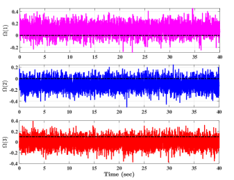
Figure 2: Angular velocity: true (black center-line) and measured (colored)

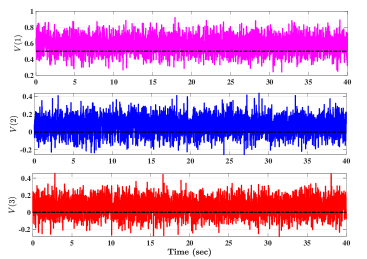
Figure 3: Translational velocity: true (black center-line) and measured (colored)

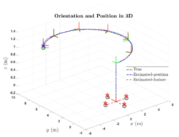
Figure 4: Simultaneous localization and mapping

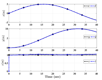
Figure 5: Position trajectory: x, y, and z

V Conclusion

In this paper, the SLAM estimation problem has been addressed in a stochastic sense. A nonlinear stochastic observer posed on the Lie Group of $\mathbb{SLAM}_{n}\left(3\right)$ has been proposed. The proposed observer can operate using angular and translational velocity measurements, along with the available feature measurements obtained from a vision unit. It has been assumed that the angular and translational velocity measurements are corrupted, not only with an unknown, constant bias, but also with a random Gaussian noise. The closed loop error signals have been shown to be semi-globally uniformly ultimately bounded. Finally, simulation results showed the effectiveness and robustness of the proposed approach given high level of uncertainties in the measurements.

References

• [1] H. A. Hashim, “GPS-denied navigation: Attitude, position, linear velocity, and gravity estimation with nonlinear stochastic observer,” in 2021 American Control Conference (ACC).   IEEE, 2021, pp. 1146–1151.
• [2] H. A. Hashim, M. Abouheaf, and M. A. Abido, “Geometric stochastic filter with guaranteed performance for autonomous navigation based on IMU and feature sensor fusion,” Control Engineering Practice, vol. PP, no. PP, pp. 1–11, 2021.
• [3] J. Guo, Y. He, X. Qi, G. Wu, Y. Hu, B. Li, and J. Zhang, “Real-time measurement and estimation of the 3d geometry and motion parameters for spatially unknown moving targets,” Aerospace Science and Technology, vol. 97, p. 105619, 2020.
• [4] H. Durrant-Whyte and T. Bailey, “Simultaneous localization and mapping: part i,” IEEE robotics & automation magazine, vol. 13, no. 2, pp. 99–110, 2006.
• [5] H. A. Hashim, “A geometric nonlinear stochastic filter for simultaneous localization and mapping,” Aerospace Science and Technology, vol. 111, p. 106569, 2021.
• [6] V. Sazdovski, A. Kitanov, and I. Petrovic, “Implicit observation model for vision aided inertial navigation of aerial vehicles using single camera vector observations,” Aerospace science and technology, vol. 40, pp. 33–46, 2015.
• [7] H. A. Hashim, “Guaranteed performance nonlinear observer for simultaneous localization and mapping,” IEEE Control Systems Letters, vol. 5, no. 1, pp. 91–96, 2021.
• [8] D. E. Zlotnik and J. R. Forbes, “Gradient-based observer for simultaneous localization and mapping,” IEEE Transactions on Automatic Control, vol. 63, no. 12, pp. 4338–4344, 2018.
• [9] M. Li and B. Xu, “Autonomous orbit and attitude determination for earth satellites using images of regular-shaped ground objects,” Aerospace Science and Technology, vol. 80, pp. 192–202, 2018.
• [10] M. J. Milford and G. F. Wyeth, “Mapping a suburb with a single camera using a biologically inspired slam system,” IEEE Transactions on Robotics, vol. 24, no. 5, pp. 1038–1053, 2008.
• [11] R. Sim, P. Elinas, and J. J. Little, “A study of the rao-blackwellised particle filter for efficient and accurate vision-based slam,” International Journal of Computer Vision, vol. 74, no. 3, pp. 303–318, 2007.
• [12] H. A. Hashim and A. E. E. Eltoukhy, “Nonlinear filter for simultaneous localization and mapping on a matrix lie group using IMU and feature measurements,” IEEE Transactions on Systems, Man, and Cybernetics: Systems, vol. PP, no. PP, pp. 1–12, 2021.
• [13] R. O. Castle, G. Klein, and D. W. Murray, “Combining monoslam with object recognition for scene augmentation using a wearable camera,” Image and Vision Computing, vol. 28, no. 11, pp. 1548–1556, 2010.
• [14] Q.-L. Li, Y. Song, and Z.-G. Hou, “Neural network based fastslam for autonomous robots in unknown environments,” Neurocomputing, vol. 165, pp. 99–110, 2015.
• [15] F. Bai, T. Vidal-Calleja, and S. Huang, “Robust incremental slam under constrained optimization formulation,” IEEE Robotics and Automation Letters, vol. 3, no. 2, pp. 1207–1214, 2018.
• [16] T. Whelan, M. Kaess, H. Johannsson, M. Fallon, J. J. Leonard, and J. McDonald, “Real-time large-scale dense rgb-d slam with volumetric fusion,” The International Journal of Robotics Research, vol. 34, no. 4-5, pp. 598–626, 2015.
• [17] J. Cheng, J. Kim, Z. Jiang, and X. Yang, “Compressed unscented kalman filter-based slam,” in 2014 IEEE International Conference on Robotics and Biomimetics (ROBIO 2014).   IEEE, 2014, pp. 1602–1607.
• [18] H. A. Hashim and A. E. E. Eltoukhy, “Landmark and IMU data fusion: Systematic convergence geometric nonlinear observer for SLAM and velocity bias,” IEEE Transactions on Intelligent Transportation Systems, vol. PP, no. PP, pp. 1–10, 2020.
• [19] J. Nielsen and R. Beard, “Ground target tracking using a monocular camera and imu in a nonlinear observer slam framework,” in 2018 Annual American Control Conference (ACC).   IEEE, 2018, pp. 6457–6462.
• [20] H. A. Hashim and F. L. Lewis, “Nonlinear stochastic estimators on the special euclidean group SE(3) using uncertain IMU and vision measurements,” IEEE Transactions on Systems, Man, and Cybernetics: Systems, vol. PP, no. PP, pp. 1–14, 2020.
• [21] H. A. Hashim, “Systematic convergence of nonlinear stochastic estimators on the special orthogonal group SO(3),” International Journal of Robust and Nonlinear Control, vol. 30, no. 10, pp. 3848–3870, 2020.
• [22] A. Odry, R. Fuller, I. J. Rudas, and P. Odry, “Kalman filter for mobile-robot attitude estimation: Novel optimized and adaptive solutions,” Mechanical systems and signal processing, vol. 110, pp. 569–589, 2018.
• [23] A. Odry, “An open-source test environment for effective development of marg-based algorithms,” Sensors, vol. 21, no. 4, p. 1183, 2021.
• [24] A. E. Eltoukhy, Z. Wang, F. T. Chan, and S. H. Chung, “Joint optimization using a leader–follower stackelberg game for coordinated configuration of stochastic operational aircraft maintenance routing and maintenance staffing,” Computers & Industrial Engineering, vol. 125, pp. 46–68, 2018.
• [25] A. E. Eltoukhy, Z. Wang, F. T. Chan, S. H. Chung, H.-L. Ma, and X. Wang, “Robust aircraft maintenance routing problem using a turn-around time reduction approach,” IEEE Transactions on Systems, Man, and Cybernetics: Systems, vol. 50, no. 12, pp. 4919–4932, 2019.
• [26] K. Ito and K. M. Rao, Lectures on stochastic processes.   Tata institute of fundamental research, 1984, vol. 24.
• [27] H. Deng, M. Krstic, and R. J. Williams, “Stabilization of stochastic nonlinear systems driven by noise of unknown covariance,” IEEE Transactions on Automatic Control, vol. 46, no. 8, pp. 1237–1253, 2001.
• [28] H. A. Hashim, L. J. Brown, and K. McIsaac, “Nonlinear stochastic attitude filters on the special orthogonal group 3: Ito and Stratonovich,” IEEE Transactions on Systems, Man, and Cybernetics: Systems, vol. 49, no. 9, pp. 1853–1865, 2019.