Scar states in a system of interacting chiral fermions

Abstract

We study the nature of many-body eigenstates of a system of interacting chiral spinless fermions on a ring. We find a coexistence of fermionic and bosonic types of eigenstates in parts of the many-body spectrum. Some bosonic eigenstates, native to the strong interaction limit, persist at intermediate and weak couplings, enabling persistent density oscillations in the system, despite it being far from integrability.

I Introduction

According to the Eigenstate Thermalization Hypothesis (ETH) Deutsch (1991); Srednicki (1994) the thermodynamic microcanonical expectation value of a physical observable (a few-body local operator) of a chaotic system can be obtained by taking a quantum expectation value of that operator in any eigenstate at the corresponding energy. To wit, all energy eigenstates are equally good at encoding thermodynamics.

ETH was presumed to universally apply to general chaotic (nonintegrable) many-body systems D’Alessio et al. (2016). Recent experimental observation of non-ergodic dynamics in a non-integrable system of interacting Rydberg atoms Bernien et al. (2017) has called the universality of ETH into question. Since then a number of models have been constructed that clearly demonstrated the possibility of weak violation of ETH, wherein most of the eigenstates satisfy ETH, but a small subset of states throughout the spectrum do not Turner et al. (2018); Moudgalya et al. (2018a); Ho et al. (2019); Iadecola et al. (2019); Lin and Motrunich (2019); Pai and Pretko (2019); Ok et al. (2019); Moudgalya et al. (2020a); Bull et al. (2019); Lee et al. (2020); Zhao et al. (2020); Bull et al. (2020); van Voorden et al. (2020); Hudomal et al. (2020); Moudgalya et al. (2020b); O’Dea et al. (2020); Mark et al. (2020); Moudgalya et al. (2020b); Srivatsa et al. (2020). These special states typically have suppressed quantum entanglement, and sometimes are equally spaced in energy, allowing their superpositions to experience perfect revivals. In the latter case, macrosocopic observables can also show oscillations in time, something not expected in ergodic thermalizing systems. These oscillations mirror behavior sometimes encountered in single-particle chaotic billiards: upon quantization, classical unstable periodic trajectories engender sequences of spectrally equidistant eigenstates, with the probability density concentrated around their “parent” classical trajectories—a phenomenon termed quantum scarring Heller (1984). Superpositions of these scarred eigenstates can capture periodic motion of wavepackets. This analogy has earned the corresponding many body states the name Quantum Many-Body Scars (QMBS). Note that not only QMBS are equidistant in energy, but their low entanglement (proximity to simple product states) reinforce the analogy with the semiclassical single-body scars.

More recently, the term QMBS has come to denote any state, even if it is not a part of an equidistant in energy sequence (“tower”) as long as it is atypical, and thus violates ETH. Several not mutually exclusive mechanisms for QMBS formation have been recognized Serbyn et al. (2020). All of them rely on the existence of exactly (or almost exactly) isolated subspace spanned by a subset of the eigenstates that share a special property, for example, a higher symmetry. Yet, the complete understanding of the origin of QMBS and their effects on macroscopic dynamics are still lacking. The fact that some nonintegrable systems show long-lived periodic dynamics raises a question whether these systems are close to some integrable point Khemani et al. (2019); Shibata et al. (2020). While certainly not necessary for the existence of generalized QMBS obtained by spectral embedding Shiraishi and Mori (2017), in some cases this remains a viable possibility.

In this paper we consider one of the simplest physical systems—chiral interacting spinless fermions confined to move on a circle of finite length $L$—to glean a possible relationship between integrability and scarring. This model is inspired by the physics of a quantum Hall droplet. The limiting cases of zero and infinite interactions correspond to free fermionic and bosonic excitations, respectively, and are trivially integrable. However, for general interactions and fermion dispersion the model is certainly nonintegrable and thus should be expected to satisfy ETH. What makes this model also interesting is that the eigenstates in the two extreme integrable limits are fundamentally different: fermionic for zero interactions, and bosonic for infinite interactions. The central result of this work is that energies of the bosonic and fermionic states at the upper edge of the spectrum (for a fixed value of the total momentum $P=2\pi n/L$, where $n$ is integer) intersect as a function of interaction strength. This immediately implies simultaneous presence of bosonic and fermionic states at intermediate couplings at least in part of the spectrum. Given that the fermionic and bosonic states are qualitatively different, but simultaneously present in the same spectral region, the strong version of ETH, which assumes that all eigenstates are qualitatively the same, is automatically violated.

For infinitely strong repulsive interactions, the anti-ground (i.e., the highest energy) state corresponds to multiple excitations occupying the lowest-momentum bosonic mode, $(b_{1}^{\dagger})^{n}|0\rangle$ (see Sec. II for details). Tracking the whole sequence for different values of $P$, we find that these states form a tower of states with the energy spacing given approximately by the energy of a single $b_{1}$ boson, even for finite interactions where these states are no longer anti-ground states. This is analogous to the exact scar states of the form $\sim(Q^{\dagger})^{n}|0\rangle$ generated by repeated applications of an operator $Q^{\dagger}$ to some reference eigenstate, previously identified in generalizations of the Hubbard model Mark and Motrunich (2020); Moudgalya et al. (2020b) and some spin models Moudgalya et al. (2018b); Schecter and Iadecola (2019).

In addition to the highest energy bosonic state, we find that descendants of other bosonic states can also survive on the nominally fermionic weak-coupling side. Similarly, the descendants of the fermionic states show persistence on the nominally bosonic side, within the same model. This indicates a distinct mechanism of QMBS, that is governed by proximity to two integrable regimes, with a phase transition separating them.

The rest of the paper is organized as follows. In Sec. II we specify the model, expressing it in two equivalent languages: fermionic and bosonic. In Sec. III we evaluate the energies of the ground and anti-ground states in the regimes of the weak and strong interactions. Surprisingly, we find that the ranges of validity of these expansions overlap for the anti-ground state in a fixed total momentum sector, which leads us to the conclusion that scar states must exist near the upper boundary of the spectrum. In Sec. IV we present numerical results that corroborate our analytical perturbative results, but also reveal QMBS in the parts of the spectrum not readily accessible analytically. In Sec. V we describe an experimentally feasible way to detect QMBS. In Sec. VI we summarize our findings, their implications for thermalization in quantum chaotic systems and possible future directions.

II The model

We consider a model of interacting spinless chiral fermions on a ring. The noninteracting dispersion $\epsilon_{k}$ with the dominant linear part $v_{0}k$ and local parabolic curvature is shown in Fig. 1(a). Throughout this paper we assume the conservation of the total momentum $P$. In this case the linear part of $\epsilon_{k}$ gives a constant contribution $v_{0}P$ to the total energy and does not affect the eigenstates of the system. We therefore omit the $v_{0}k$ part of the dispersion in the rest of the paper, see Fig. 1(b). Despite the shift of energies, the occupancies in the ground state remain the same as in the Fig. 1(a).

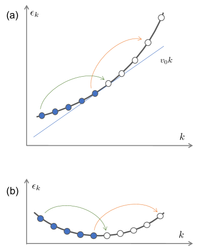
Figure 1: Chiral fermion dispersion and excitations. (a) Physical spectrum is mostly linear, with a parabolic correction. In the ground state, all states with momentum $k$ below a Fermi momentum are filled, while the rest are empty. At fixed total momentum $P$, the slope of the dispersion at the Fermi level, $v_{0}$, gives only a constant contribution $v_{0}P$ to the Hamiltonian, and thus can be ignored. This leads to a simple parabolic dispersion near the Fermi level (panel b). The orange and green arrows show particle and hole excitations (with momentum 5 in this case).

As the first step, to make the problem dimensionless, we take the circumference $L=2\pi$ and $\hbar=m=1$. This corresponds to energy being measured in the units of $4\pi^{2}\hbar^{2}/(mL^{2})$. The momentum of each fermion is given by an integer number, $k=0,\pm 1,\pm 2,\ldots$, and the Hamiltonian of the free fermions has the form

$$H_{F}=\sum_{k}\epsilon_{k}a_{k}^{\dagger}a_{k},\quad\epsilon_{k}=\frac{1}{2}\left(k-\frac{1}{2}\right)^{2}.$$ (1)

Here $a_{k}^{\dagger}$ is the creation operator for a fermion with momentum $k$.

The simplest eigenstate of $H_{F}$ corresponds to all single particle states with $k\leq 0$ being filled, and those with $k>0$ empty, see Fig. 1. We denote this state $|0\rangle$ and measure the total momentum $P$ of any state from its value at $|0\rangle$. It is easy to see that there is only one state in $P=1$ sector, $a^{\dagger}_{1}a_{0}|0\rangle$, which corresponds to taking a fermion from the state $k=0$ and moving it to $k=1$. In contrast, there are multiple fermionic states in sectors with $P>1$. Taken as product states (Fock basis), they are eigenstates of $H_{F}$. However, interactions generate mixing among them.

We consider the usual two-body interactions between fermions, which in a translation invariant system are described by the Hamiltonian

$$H_{B}=\sum_{\begin{subarray}{c}k_{1}k_{2}\\ q>0\end{subarray}}V(q)a_{k_{1}+q}^{\dagger}a_{k_{1}}a_{k_{2}}^{\dagger}a_{k_{2}+q},$$ (2)

for which $H_{B}|0\rangle=0$. To achieve the latter condition we have subtracted from the standard normal-ordered expression an operator that at fixed number of particles amounts to a constant. In addition, in Eq. (2) we omitted the $1/L=1/2\pi$ prefactor, subsuming it in the definition of the Fourier transform $V(q)$ of the interaction potential.

In the limit of strong interactions, it is convenient to bosonize the Hamiltonians (1) and (2). Bosonic operators $b_{q}$ are expressed in terms of the fermionic ones as Haldane (1981)

$$b_{q}=\frac{1}{\sqrt{q}}\sum_{k}a_{k}^{\dagger}a_{k+q},\quad b_{q}^{\dagger}=\frac{1}{\sqrt{q}}\sum_{k}a_{k+q}^{\dagger}a_{k},$$ (3)

where the momentum $q$ of the boson is a positive integer. Using Eq. (3), one can rewrite the interaction Hamiltonian (2) as

$$H_{B}=\sum_{q=1}^{\infty}\varepsilon_{q}b_{q}^{\dagger}b_{q},\quad\varepsilon_{q}=qV(q).$$ (4)

The main advantage of bosonization is that Hamiltonian (4) is quadratic in bosonic variables. The disadvantage is that in terms of the bosonic variables the Hamiltonian $H_{F}$ is no longer quadratic Haldane (1981),

$$H_{F}=\frac{1}{12\pi}\int_{0}^{2\pi}[\phi^{\prime}(x)]^{3}dx,$$ (5)

where the bosonic field $\phi(x)$ is defined as

$$\phi(x)=-i\sum_{q=1}^{\infty}\frac{1}{\sqrt{q}}(b_{q}e^{iqx}-b_{q}^{\dagger}e^{-iqx}).$$ (6)

Substituting this expression into Eq. (5), we obtain

$$H_{F}=\frac{1}{2}\sum_{q=2}^{\infty}\sum_{q^{\prime}=1}^{q-1}\sqrt{qq^{\prime}(q-q^{\prime})}\left(b_{q}^{\dagger}b_{q^{\prime}}b_{q-q^{\prime}}+b_{q^{\prime}}^{\dagger}b_{q-q^{\prime}}^{\dagger}b_{q}\right).$$ (7)

In the bosonic representation, the fully occupied Fermi sea $|0\rangle$ corresponds to the bosonic vacuum. The only fermionic state $a^{\dagger}_{1}a_{0}|0\rangle$ in the $P=1$ sector corresponds to $b_{1}^{\dagger}|0\rangle$ state in the bosonic representation. Despite very different representations, the number of states in a given sector $P$ does not depend on the basis Haldane (1981). One can easily verify explicitly that the expressions (1) and (7) give the same excitation spectrum for the system of free fermions for a few small values of the total momentum $P$.

Bosonic basis provides a simple way to count the number of states per sector. It is given by the number of distinct integer partitions of $P$, i.e., the number of distinct sets of non-negative integers $\{n_{q}\}$, with $q=1,\ldots,P$ such that $\sum_{q}q\,n_{q}=P$. Physically, $q$ is the momentum of a bosonic mode, and $n_{q}$ is its occupation number. For large total momentum, $P\gg 1$, the dimensionality of the symmetry sector scales as $\frac{1}{4\sqrt{3}P}\exp\left(\pi\sqrt{\frac{2P}{3}}\right)$, Ref. Hardy and Ramanujan (1918). We have been able to compute all eigenstates for $P\leq 38$, and some eigenstates for $P$ up to 72, which allowed us to numerically test analytical findings. The computations can be performed in both the bosonic or fermionic bases. The numerical results presented in Sec. IV are obtained in the bosonic basis.

In this paper we will concern ourselves primarily with unscreened Coulomb interaction between fermions, which we define as $V(x)\propto\sum_{n=-\infty}^{\infty}1/|x-2\pi n|$ to account for the periodic boundary conditions. The Fourier transform of this interaction potential has the form

$$V(q)=-V_{0}\ln|q|.$$ (8)

Just like the individual momenta of electrons, for $L=2\pi$, the relevant momentum transfers $q$ are limited to integers. In Eq. (8) we have shifted $V(q)$ by a constant in order to have $V(1)=0$. This shift is equivalent to subtracting a value proportional to $P$ from the Hamiltonian, which does not affect the eigenstates and relative positions of the energy levels for a given interaction.

III Crossover between the regimes of weak and strong interactions

In this section we provide analytical results for some eigenstates in the intermediate coupling regime based on the weak and strong coupling expansions. Most importantly, we demonstrate that the ranges of validity of the two expansions can overlap. The weak coupling expansion perturbatively modifies fermionic product states, and the strong coupling expansion does the same to bosonic states. The overlap thus implies that there is a range of interactions where fermionic and bosonic types of states coexist. The states of one type in a region dominated by those of the other type represent scar states in our model.

Let us consider the states in the sector with total momentum $P$ relative to the fully occupied Fermi sea state, corresponding to $P=0$. In the case of free fermions, $V_{0}=0$, described by the Hamiltonian (1), each state has a number of particle and hole excitations, with the total momentum $P$. Due to the convexity of the kinetic energy, the upper and lower boundaries of the energy spectrum are achieved for the states

$$\psi_{F}^{(u)}=a_{P}^{\dagger}a_{0}|0\rangle,\quad\psi_{F}^{(l)}=a_{1}^{\dagger}a_{1-P}|0\rangle.$$ (9)

They correspond to a single particle and a single hole excitations, respectively. (These are the states that are obtained from the fully occupied Fermi sea via processes shows by green and orange arrows in Fig. 1.) The energies of these states are

$$E_{F}^{(u)}=\frac{P(P-1)}{2},\quad E_{F}^{(l)}=-\frac{P(P-1)}{2}.$$ (10)

(Hereinafter the energies of all states are measured from that of state $|0\rangle$.) In the opposite limit of strong interactions, $V_{0}\to+\infty$, one can neglect $H_{F}$ compared to $H_{B}$, and use the form (4) of the latter to determine the boundaries of the excitation spectrum. The states with the highest and lowest energies are

$$\psi_{B}^{(u)}=\frac{1}{\sqrt{P!}}(b_{1}^{\dagger})^{P}|0\rangle,\quad\psi_{B}^{(l)}=b_{P}^{\dagger}|0\rangle.$$ (11)

Their energies are

$$E_{B}^{(u)}=0,\quad E_{B}^{(l)}=-V_{0}P\ln P.$$ (12)

As we see, these spectral boundary states, both in the fermionic and bosonic limits correspond to very simple states. Next we use perturbation theory to obtain the shapes of the upper and lower boundaries of the spectrum in the regimes of weak and strong interactions (see Fig. 2 below). This will enable us to obtain the scale of the interaction parameter $V_{0}$ at which the crossover occurs and to discuss its nature.

III.1 Weak interaction regime

We start by evaluating the first order correction to the fermionic anti-ground state energy $E^{(u)}_{F}$ in the case of weak interactions. To this level of approximation the correction to the energy of the system is obtained by evaluation of the expectation value of the interaction Hamiltonian (2) in a state with $n_{k}=\langle a_{k}^{\dagger}a_{k}\rangle$ taking values 0 or 1. This procedure yields

$$\delta_{1}E_{F}=\sum_{k,k^{\prime}}n_{k}(1-n_{k^{\prime}})V(k-k^{\prime})\theta(k-k^{\prime}),$$ (13)

where the unit step function $\theta(x)$ is defined such that $\theta(0)=0$. The sum here is performed over all integer $k$ and $k^{\prime}$.

The state with the highest possible energy at a given momentum $P$ is obtained from the ground state by moving a fermion from $k=0$ to $k=P$, cf. Eq. (9) (also orange arrow in Fig. 1). For this state only the $P$ terms, for which $k=P$ and $k^{\prime}=0,1,\ldots,P-1$ contribute to Eq. (13), resulting in

$$\delta_{1}E_{F}^{(u)}=\sum_{q=1}^{P}V(q),$$ (14)

For the Coulomb interaction $V(q)$ is given by Eq. (8), and we find

$$\delta_{1}E_{F}^{(u)}=-V_{0}\ln(P!).$$ (15)

Repeating the same calculation for the lowest energy state $\psi_{F}^{(l)}$, obtained by introducing a single hole with momentum $P$, see Eq. (9) (also green arrow in Fig. 1), we find the same result,

$$\delta_{1}E_{F}^{(l)}=-V_{0}\ln(P!).$$ (16)

In the most important regime of $P\gg 1$, the results (15) and (16) scale as

$$\delta_{1}E_{F}^{(u)}=\delta_{1}E_{F}^{(l)}\simeq-V_{0}P(\ln P-1).$$ (17)

The second order correction to the energy of the anti-ground state at weak interactions is

$$\delta_{2}E_{F}^{(u)}=\sum_{q=1}^{P-1}\sum_{k=0}^{q-1}\frac{(V(q)-V(P-k))^{2}}{q(p-k)}\theta(P-q-k).$$ (18)

For the Coulomb interaction (8) we obtain

$$\delta_{2}E_{F}^{(u)}=c(P)V_{0}^{2},$$ (19)

where

$$c(P)=\sum_{q=1}^{P-1}\sum_{k=0}^{q-1}\frac{\ln^{2}\frac{q}{P-k}}{q(P-k)}\theta(P-q-k).$$ (20)

Repeating the evaluation for the single-hole state $\psi_{F}^{(l)}$, one obtains

$$\delta_{2}E_{F}^{(l)}=-c(P)V_{0}^{2}.$$ (21)

At large momentum $c(P)$ defined by Eq. (20) approaches the limit $c(\infty)=7\pi^{4}/360$ one .

III.2 Strong interaction regime

We now study the energies of the ground and anti-ground states in the regime of strong interactions. To first approximation one can neglect the term $H_{F}$ that does not contain the large parameter $V_{0}$ and obtain the energies given by Eq. (12). Next we find the leading order correction to the ground state energy $E_{B}^{(l)}$ in the perturbation (7). Clearly, the first-order correction $\langle\psi_{B}^{(l)}|H_{F}|\psi_{B}^{(l)}\rangle=0$. The second-order correction to the energy is

$$\delta E_{B}^{(l)}=\frac{1}{2}\sum_{q=1}^{P-1}\frac{Pq(P-q)}{\varepsilon_{P}-\varepsilon_{q}-\varepsilon_{P-q}}.$$ (22)

Substituting the expression $\varepsilon_{q}=-V_{0}q\ln q$, we obtain

$$\delta E_{B}^{(l)}=-\gamma(P)\frac{P^{3}}{V_{0}},$$ (23)

where

$$\gamma(P)=\frac{1}{2P^{2}}\sum_{q=1}^{P-1}\frac{q(P-q)}{q\ln\frac{P}{q}+(P-q)\ln\frac{P}{P-q}}.$$ (24)

At large $P$ the function $\gamma(P)$ approaches a finite value, $\gamma(\infty)\approx 0.15743$ one .

To first approximation the energy of the anti-ground state $E_{B}^{(u)}$ given by Eq. (12) vanishes. The leading order expression for $E_{B}^{(u)}$ is obtained in the second order perturbation theory in the operator $H_{F}$ given by Eq. (7). An important difference between the wavefunctions of the ground and anti-ground states is that the latter has a single boson state with the large occupation number $P$, see Eq. (11). To properly account for the large occupation of bosonic states involved in the perturbation theory, we introduce $|n_{1},n_{2},n_{3},\ldots\rangle$ as the properly normalized state in which for $q=1,2,3,\ldots$ the bosonic modes with momentum $q$ are occupied by $n_{q}$ bosons. At $V_{0}=\infty$, the anti-ground state $\psi_{B}^{(u)}$ is then written as $|P,0,0,\ldots\rangle$. To first order in $H_{F}$, it couples only to the state $|P-2,1,0,\ldots\rangle$, with the matrix element

$$t_{12}=\langle P-2,1,0,\ldots|H_{F}|P,0,0,\ldots\rangle=\sqrt{\frac{P(P-1)}{2}},$$ (25)

see Eq. (7). The first order correction to wavefunction results in the second-order correction to the energy, $t_{12}^{2}/(-\varepsilon_{2})$, which in the case of Coulomb interaction takes the form

$$E_{B}^{(u)}=\frac{P(P-1)}{4\ln 2\,V_{0}}.$$ (26)

To determine the range of applicability of this result, we next find the first subleading correction to $E_{B}^{(u)}$.

In second order in $H_{F}$ for the wave function, two additional states become coupled to $|P,0,0,\ldots\rangle$. First, one can transfer two more bosons from mode 1 to mode 2, yielding $|P-4,2,0,\ldots\rangle$. The corresponding matrix element is

$$\tilde{t}_{12} = \langle P-4,2,0,\ldots|H_{F}|P-2,1,0,\ldots\rangle$$ (27)

$$= \sqrt{(P-2)(P-3)}.$$

Second, a boson can be transferred from mode 2 to mode 3, while also removing one boson from mode 1. The corresponding matrix element is

$$t_{23} = \langle P-3,0,1,\ldots|H_{F}|P-2,1,0,\ldots\rangle$$ (28)

$$= \sqrt{6(P-2)}.$$

Using the above expressions, the energy up to the fourth order has the form

$$E_{B}^{(u)}=-\frac{t_{12}^{2}}{\varepsilon_{2}}+\frac{t_{12}^{2}\left(2t_{12}^{2}-\tilde{t}_{12}^{2}\right)}{2\varepsilon_{2}^{3}}-\frac{t_{12}^{2}t_{23}^{2}}{\varepsilon_{2}^{2}\varepsilon_{3}},$$

which for Coulomb interaction results in

$$E_{B}^{(u)}=\frac{P(P-1)}{4\ln 2\,V_{0}}+\left[\frac{P-2}{4(\ln 2)^{2}\ln 3}-\frac{2P-3}{16(\ln 2)^{3}}\right]\frac{P(P-1)}{V_{0}^{3}}.$$ (29)

The second term here is small compared to the first one as long as $V_{0}\gg\sqrt{P}$.

To gain better insight into the nature of the anti-ground state at strong interactions, let us consider the limiting procedure in which $P\to\infty$, while $V_{0}/P$ remains finite. In this limit one can simplify Eqs. (25) and (27) and approximate $t_{12}=P/\sqrt{2}$ and $\tilde{t}_{12}=P$. This approximation can be understood as replacing $(b_{2}^{\dagger}b_{1}b_{1}+b_{1}^{\dagger}b_{1}^{\dagger}b_{2})\to P(b_{2}^{\dagger}+b_{2})$ in the perturbation operator (7). The other terms in Eq. (7) contain at most one operator $b_{1}$ or $b_{1}^{\dagger}$, which means that they are proportional to at most $\sqrt{P}$ and can be neglected in comparison. This corresponds to replacing the full Hamiltonian $H_{B}+H_{F}$ with the effective Hamiltonian

$$H_{\rm eff}=\varepsilon_{2}[b_{2}^{\dagger}b_{2}+\lambda(b_{2}^{\dagger}+b_{2})],$$ (30)

where

$$\lambda=\frac{P}{\sqrt{2}\,\varepsilon_{2}}.$$ (31)

The Hamiltonian $H_{\rm eff}$ is easily diagonalized,

$$H_{\rm eff}={\varepsilon_{2}}b^{\dagger}b-\lambda^{2}{\varepsilon_{2}}.$$ (32)

Here the new bosonic operator $b$ is defined by

$$b=b_{2}+\lambda.$$ (33)

Physically, $\lambda$ is the constant displacement of mode 2 induced by the bosonic “condensate” in mode 1. The corresponding vacuum energy of mode 2, given by the constant term in Eq. (32), becomes the energy of the anti-ground state that we seek,

$$E_{B}^{(u)}=-\lambda^{2}{\varepsilon_{2}}=\frac{P^{2}}{4\ln 2\,V_{0}},$$ (34)

At $P\to\infty$, this expression is indeed identical to the first term of Eq. (29), but unlike the latter, our result (34) does not rely on the perturbative expansion of $E_{B}^{(u)}$ in the coupling matrix element (25).

The applicability of this approach is limited by the condition that the terms $b_{2}^{\dagger}b_{1}b_{1}$ and $b_{1}^{\dagger}b_{1}^{\dagger}b_{2}$ in the perturbation (7) are dominant. This holds as long as the occupation of the first bosonic state $\langle b_{1}^{\dagger}b_{1}\rangle\sim P$ is much larger that that of any other state. Given the form of the Hamiltonian (30), the second most occupied bosonic state has momentum $q=2$. Its occupation $\langle b_{2}^{\dagger}b_{2}\rangle$ in the vacuum state of the operator $b$ is

$$\langle b_{2}^{\dagger}b_{2}\rangle=\lambda^{2}=\frac{1}{8\ln^{2}2}\left(\frac{P}{V_{0}}\right)^{2},$$ (35)

where we used Eq. (33). Thus the condition $\langle b_{2}^{\dagger}b_{2}\rangle\ll\langle b_{1}^{\dagger}b_{1}\rangle\sim P$ is satisfied as long as $V_{0}\gg\sqrt{P}$. This condition coincides with the one obtained earlier from the perturbation theory.

Before closing this section, we compute the overlap of the vacuum states of the operators $b$ and $b_{2}$. This overlap plays an important role in determining whether an external drive that induces transition between anti-ground states in different $P$ sectors also changes the occupancy of the $b_{2}$ mode. To obtain it, we represent $b_{2}$ as the differential operator

$$b_{2}=\frac{1}{\sqrt{2}}\left(x+\frac{d}{dx}\right)$$ (36)

in the space of functions $\psi(x)$ of a real variable $x$. It is easy to verify that the commutator $[b_{2},b_{2}^{\dagger}]=1$. The vacuum state $\psi_{0}(x)$ of the operator $b$ is then defined by

$$\left[\frac{1}{\sqrt{2}}\left(x+\frac{d}{dx}\right)+\lambda\right]\psi_{0}(x)=0.$$

This first order differential equation is easily solved,

$$\psi_{0}(x)=\frac{1}{\sqrt[4]{\pi}}\exp\left(-\frac{1}{2}(x+\sqrt{2}\lambda)^{2}\right).$$ (37)

Here we applied the normalization condition $\langle\psi|\psi\rangle=1$, where

$$\langle\phi|\psi\rangle=\int_{-\infty}^{\infty}\phi^{*}(x)\psi(x)dx.$$

The vacuum state $\phi_{0}(x)$ of the operator $b_{2}$ is obtained by setting $\lambda=0$ in Eq. (37). The overlap $\langle\phi_{0}|\psi_{0}\rangle$ is then obtained as

$$\langle\phi_{0}|\psi_{0}\rangle=e^{-\lambda^{2}/2}=\exp\left[-\frac{1}{16\ln^{2}2}\left(\frac{P}{V_{0}}\right)^{2}\right].$$ (38)

This result will be used in Section V.

III.3 Upper and lower edges of the spectrum at $P\gg 1$

Next, we summarize the overall behavior at the spectral edges in the full range of interactions. At $P\gg 1$ the lower edge of the spectrum for weak interactions is given by

$$E^{(l)}_{F}=-\frac{P^{2}}{2}-V_{0}P(\ln P-1)-\frac{7\pi^{4}}{360}V_{0}^{2},$$ (39)

where we combined our earlier results (10), (17), and (21). For strong interactions, the lower edge is obtained by combining Eqs. (12) and (23),

$$E^{(l)}_{B}=-V_{0}P\ln P-\gamma(\infty)\frac{P^{3}}{V_{0}}.$$ (40)

The term $-V_{0}P\ln P$ appears at both small and large $V_{0}$. The remaining terms in both Eqs. (39) and (40) are of the same order of magnitude at $V_{0}\sim P$. One should therefore expect a smooth crossover between the two regimes at $V_{0}\sim P$.

For the upper spectral edge, at weak interactions we have

$$E^{(u)}_{F}=\frac{P^{2}}{2}-V_{0}P(\ln P-1)+\frac{7\pi^{4}}{360}V_{0}^{2},$$ (41)

where we combined the results (10), (17), and (19). For strong interactions, to leading order in $1/V_{0}$, we have

$$E^{(u)}_{B}=\frac{P^{2}}{4\ln 2\,V_{0}},$$ (42)

cf. Eqs. (26) and (34). We omitted the corrections to the leading contribution (42) found in Eq. (29), which limits the applicability of Eq. (42) to $V_{0}\gg\sqrt{P}$.

Let us consider the regime of moderately strong interactions, $V_{0}\sim V^{*}$, where

$$V^{*}=\frac{P}{2\ln P}.$$ (43)

For such interactions the last term of Eq. (41) is negligible, while the first two terms yield $E_{F}^{(u)}\sim P^{2}$. On the other hand, Eq. (42) yields $E_{B}^{(u)}\sim P\ln P\ll P^{2}$. At the energy scales of the order of $P^{2}$ one can then approximate $E_{B}^{(u)}=0$. This gives the true upper boundary of the spectrum at sufficiently large interactions, where $E_{F}^{(u)}$ becomes negative. Summarizing the above findings, at $P\gg 1$ we obtain

$$E^{(u)}=\frac{P^{2}}{2}\times\left\{\begin{array}[c]{ll}1-\frac{V_{0}}{V^{*}},&\mbox{at $V_{0}<V^{*}$},\\[8.61108pt] 0,&\mbox{at $V_{0}>V^{*}$}.\end{array}\right.$$ (44)

It is important to note that unlike the smooth crossover between the regimes of weak and strong interactions at the lower edge of the spectrum, at the upper one we have a sharp transition at $V_{0}=V^{*}$.

III.4 Scar states near the upper spectral edge

Interacting one-dimensional Fermi systems can be described in two complementary languages. At weak interactions the original theory in terms of weakly interacting fermions is more convenient. At strong interactions, bosonized description is preferable, as the bosons are now weakly interacting. In particular, this applies to both the ground and anti-ground states, Sec. III.3. However, we have found that the crossovers between the weakly and strongly interacting regimes are qualitatively different at the two extremes of the spectrum.

For the ground state, the smooth crossover implies that at $V_{0}\sim P$ both fermions and bosons experience strong interactions, and neither description is simpler than the other. This is not the case for the anti-ground state. We found that at $V_{0}<V^{*}$ the highest energy state is adequately described in terms of weakly interacting fermions. Conversely, at $V_{0}>V^{*}$, the anti-ground state is described most simply in the language of weakly interacting bosons. The energies of these two states are equal at $V_{0}=V^{*}$, but their nature remains very different. In other words, we conclude that at $P\gg 1$ the two levels cross at $V_{0}=V^{*}$ without significant level repulsion.

Our description of the bosonic anti-ground state in Sec. III.2 applies as long as $V_{0}>\sqrt{P}$. This state has the highest energy at $V_{0}>V^{*}$, but in the parametrically broad range of interaction strengths $\sqrt{P}\ll V_{0}<V^{*}$ it has lower energy than the fermionic anti-ground state. It is therefore embedded in the nearly continuous spectrum of states composed of weakly interacting particle-hole excitations. This behavior is analogous to that of scar states in nearly ergodic systems Lin et al. (2020).

One can similarly argue that at $V_{0}>V^{*}$ the fermionic anti-ground state enters the region of energies dominated by states composed of weakly interacting bosons. Given that the structure of the perturbation theory in small $V_{0}$ is the same for the ground and anti-ground states, we expect that the result (41) also applies as long as $V_{0}\ll P$. Thus the fermionic scar state near the upper boundary of the spectrum should be present in the logarithmically broad range $V^{*}<V_{0}\ll P$.

The qualitative difference between the crossovers for the ground and anti-ground states can be traced back to their form in the limit of strong interactions, see Eq. (11). The overlap of the single boson excitation state $\psi_{B}^{(l)}$ with $\psi_{F}^{(l)}$ given by Eq. (9) is $1/\sqrt{P}$. [This can be seen immediately from Eq. (3).] On the other hand, the state $\psi_{B}^{(u)}$ is very different in that a single bosonic state is filled with $P\gg 1$ particles. One can show that its overlap with $\psi_{F}^{(u)}$ is exponentially small at large $P$, which results in level crossing at the upper edge of the spectrum. This argument can be extended to at least a few highest energy states, which should also cross each other near $V^{*}$ at sufficiently large $P$. Thus one should expect a sequence of bosonic scar states at $V_{0}<V^{*}$ as well as several fermionic states at $V_{0}>V^{*}$. This conclusion is supported by numerical calculations, see Sec. IV.

IV Numerical results

In this section we supplement the analytical results derived in the previous sections with numerical calculations. To start off, Fig. 2, shows the general comparison between the numerically obtained upper and lower edges of the spectrum and the analytical strong- and weak-coupling perturbative expansions for $P=72$. The agreement is excellent, and the intersections of the analytical asymptotes tracks qualitative changes in the spectrum. The most notable feature is the incipient level crossing at the upper edge of the spectrum, which is indicative of QMBS. In the following subsections we carefully examine these level crossings and their dependence on the form of interaction. We use participation ratio in fermionic and bosonic bases to classify the states according to their type. This reveals that the scar states are not limited to the upper edge of the spectrum, but exist throughout, in the intermediate coupling regime.

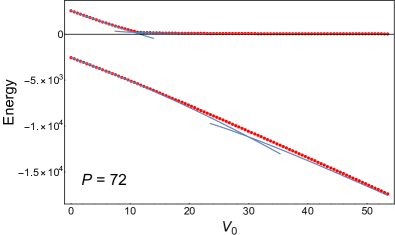
Figure 2: Upper and lower edges of the spectrum for $P=72$ obtained by numerical diagonalization of the Hamiltonian given by Eqs. (4) and (7), assuming Coulomb interaction (8). Solid lines are the results of analytical perturbation theory, see Eqs. (10), (12), (15), (16), (19), (21), (23), and (29). Note that at the lower edge of the spectrum, the crossover is at larger values of $V_{0}$ than at the upper edge.

IV.1 Level crossings

As shown analytically above, for repulsive interactions, we anticipate a level crossing between the fermionic anti-ground state originating at low interactions strengths and bosonic anti-ground state, which becomes exact in the infinite interaction limit. The crossing as a function of the interaction scale $V_{0}$ at fixed $P$ is expected to develop only as $P\to\infty$. In Fig. 3 we show three uppermost levels in the spectrum of Coulomb-interacting fermions for $P=72$. Their most noticeable feature is that levels congregate near interaction $V_{0}=11.4$. Upon closer inspection, the changes of curvature reveal that the levels undergo a pair-wise avoided level crossings. At a smaller value of the total momentum $P=38$ (inset) no avoided crossing is evident.

Though the minigaps of the avoided level crossing clearly shrink with increasing $P$, our numerical limitations do not allow us to readily access larger system sizes to see the incipient level crossing more explicitly in the case of Coulomb interaction. Fortunately, it is possible to make the underlying physics more self-evident by modifying the form of interaction. In Fig. 4 we used interaction $V(q)=V_{0}(|q|^{-1}-1)$ that scales as $\ln\frac{1}{|x|}$ in real space. (It can be viewed as a special case of the more general interaction $V(q)=V_{0}(|q|^{\alpha-1}-1)/(1-\alpha)$ corresponding to $\alpha=0$, whereas the Coulomb interaction (8) corresponds to the limit $\alpha\to 1$). Already at the moderate system size $P=38$, the minigaps become much smaller than the level spacing for the top levels, increasing gradually for deeper levels. For comparison, the inset shows the data for $P=24$, which has a level structure similar to that for a much larger value $P=72$ and Coulomb interactions.

Despite the significant quantitative difference the structure of the energy levels near the transition point for the Coulomb and logarithmic interactions, we observe no qualitative changes in the physical behavior. Given that the modified interaction is much more amenable to the numerical exploration, we limit ourselves to this case in the rest of this Section.

The level crossings are a strong indicator that some states can penetrate into the interaction regime dominated by states of different character. That is, they point to the presence of scars. Next, we verify that this is indeed the case by directly examining the character of the wavefunctions.

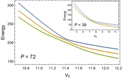
Figure 3: Coulomb interaction. Three uppermost levels as a function of the interaction strength. Main panel: total momentum sector $P=72$. Note that the second level (orange dots) has regions of positive and negative curvature, separated by two inflection points. Less obviously, third level (green dots) has four inflection points. This behavior is reflective of avoided level crossings. Inset: total momentum sector $P=38$. The data shows no avoided crossing behavior.

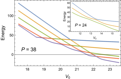
Figure 4: Logarithmic interaction. Uppermost levels as a function of interaction strength. Main panel: total momentum sector $P=38$. Compared to Fig. 3, multiple level crossings have become apparent, even at a considerably smaller value of $P$. The level repulsion is discernible only between 4th and 5th levels, or for smaller values of the total momentum, such as $P=24$ shown in the inset.

IV.2 Wavefunction character

The presence of scars is evidenced not only by the energy level crossings, but also by the character of the eignestates $|\Psi_{m}\rangle$. To demonstrate that, we expand the exact eigenstates in terms of the noninteracting (fermionic) basis states $|f_{n}\rangle$ or infinitely interacting (bosonic) basis states $|b_{n}\rangle$. We then quantify the number of the relevant states in the expansion using the corresponding participation ratios, $N_{f}(m)=1/\sum_{n}|\langle\Psi_{m}|f_{n}\rangle|^{4}$ and $N_{b}(m)=1/\sum_{n}|\langle\Psi_{m}|b_{n}\rangle|^{4}$. For states accurately represented by only a few basis states the corresponding $N$ is of order unity. On the other hand, if the full basis is needed to represent a state, then $N$ scales with the dimensionality of the Hilbert space. It is convenient to also introduce a quantity $\chi(m)=N_{b}(m)/N_{f}(m)$.

In Fig. 5 we show the spectrum of the system with logarithmic interaction in the sector $P=38$ as a function of the interaction strength, with each dot representing a state. The color indicates the character of the state: red corresponds to the fermionic character, $\chi(m)\gg 1$, blue to bosonic, $\chi(m)\ll 1$, and intermediate colors correspond to intermediate character. Since the number of states at this value of $P$ is very large (26015), the order in which the states are plotted matters. There are two particularly informative methods, which highlight the most typical or the least typical states. We first compute the deviation of $\chi(m)$ from the geometric mean $\bar{\chi}(m)$ of its 100 neighbors in energy (on both sides, at the same $V_{0}$). In the top panel, the typical states, for which $\chi(m)$ is closest to $\bar{\chi}(m)$ are plotted last. This naturally leads to a smooth pattern. In the lower panel, the outliers are plotted last, which emphasizes the atypical, scar states.

As was theoretically anticipated, bosonic-like states near the upper edge of the spectrum penetrate into the fermionic domain. Similarly, fermionic-like states can appear on the strongly coupled side that is dominated by bosonic states. Notably, there are also a number of additional scar states throughout the spectrum. More generally, the participation ratio shows that in the transition region, the fermionic and bosonic states intermix in a complicated fashion throughout the spectrum, even in a fixed total momentum sector.

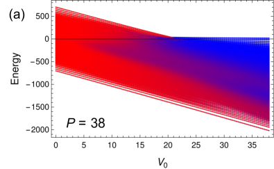
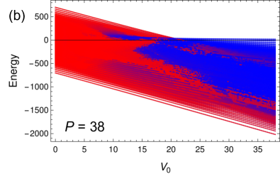
Figure 5: Character of eigenstates, as encoded by the ratio of fermionic and bosonic participation ratios. Red corresponds to fermionic character, and blue to bosonic. Panel (a) shows typical character. Panel (b) emphasizes the outliers—the states that most strongly deviate from the typical states in their vicinity. (See text for details.) Most notably, near the upper boundary of the spectrum, there is an island of atypical bosonic scar states that appears at low interactions ($V_{0}\sim 12$) and a fermionic island at large interactions ($V_{0}\sim 25$). Both appear to be the extrapolations of the corresponding states at the upper edge of the spectrum.

V Observing scars

In the previous sections we have shown that for a sufficiently large value of total momentum $P$ atypical scar states appear throughout the spectrum, most prominently in the vicinity of the upper edge. The discontinuity in slope as a function of the interaction strength indicates that for smaller interactions the states are fermionic, and for larger—bosonic in character. We now address observability of the atypical bosonic collective states in the regime of intermediate and weak interactions, where the native states are fermionic.

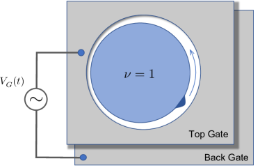
Figure 6: Interacting chiral fermions at the edge of a $\nu=1$ quantum Hall droplet. Starting from the ground state, $P=0$, atypical scar states at the upper edge of the spectrum can be excited by applying voltage $V(t)$ between the top and the back gates at the frequency that corresponds to a wavepacket (blue bump) propagation around the edge. This favors transitions between $P$ and $P+1$ anti-ground states. Selective excitation of these states is further enhanced by having the gate primarily coupled to the lowest spatial harmonic (for circular droplet shown here, the top gate is slightly offset relative to it). Once exited, voltage oscillations associated with a travelling density wave can persist for anomalously long time.

As a specific practical realization we consider a quantum Hall droplet, electrically insulated from the rest of the system, but electrostatically gated. Voltage applied between back gate and the top gate can be used to excite density modes in the droplet, and the top gate can be also used to detect excited oscillations, Fig. 6. We assume for simplicity that the dominant spatial dependence of the gate potential is harmonic with the period $L$ (as, for instance, would be the case for a circular droplet and circular gate opening surrounding it, but slightly displaced). Then, the Hamiltonian that describes the interaction between the gate and the chiral system is

$$H_{D}=D\cos(\omega_{D}t)(b_{1}+b_{1}^{\dagger}),$$ (45)

where $D$ is the drive strength and $\omega_{D}$ is the drive frequency. From Eq. (29), the upper edge of the spectrum, from the bosonic side is

$$E_{B}^{u}(P)=\frac{P(P-1)}{4\ln 2\,V_{0}}+O(P^{3}/V_{0}^{3}).$$ (46)

As explained above, these correspond to the multiboson states, $\Psi_{P}\approx(b_{1}^{\dagger})^{P}|0\rangle$. The drive Eq. (45) effectively acts as hopping on a one-dimensional lattice with sites labeled by $P$. If we assume that the drive frequency is resonant with the $P=0$ to $P=1$ transition, it will connect states up to

$$|E_{B}^{u}(P_{max})-E_{B}^{u}(0)|\lesssim\sqrt{P_{max}}D,$$ (47)

where the pefactor $\sqrt{P_{max}}$ on the right hand side is the scale of $|\langle b_{1}\rangle|$. This implies that applying drive of strength $D$ leads to excitation of multiboson anti-ground states up to

$$P_{max}(D)\sim(DV_{0})^{2/3}.$$ (48)

From Eq. (48), the drive strength needed to reach the kink ($V_{0}\sim P$) at the upper spectral edge is $D_{\rm kink}\sim V_{0}^{1/2}$.

The above assumes that the $b_{2}$ bosons are not being excited. We now verify that this is indeed the case. Referring back to Sec. III.2 and in particular the effective Hamiltonian (30), we can estimate the matrix element of the transition to states with non-zero number of excited phonons $b_{2}^{\dagger}b_{2}$. From Eq. (38), the probability to remain in the vacuum of $b_{2}$ while changing $P$ to $P+1$ is given by the Frank-Condon factor, $e^{-1/({8\ln^{2}2\,V_{0}^{2}})}$, which is close to 1 for large $V_{0}$ that we assume here. After $P$ consecutive steps, starting from $P=0$ state, this probability becomes $e^{-P/({8\ln^{2}2\,V_{0}^{2}})}$, remaining close to one as long as $P\ll V_{0}^{2}$. This is indeed the regime where the perturbation theory developed in Sec. III.2 is expected to hold. (Recall that the bosonic “scar regime” is approximately $\sqrt{P}<V_{0}<P$.) We thus conclude that the bosonic scar anti-ground state can be effectively excited, and should be observable via voltage oscillations on the gate long after the drive has been turned off.

VI Discussion and open questions

In this paper we have found evidence of quantum many-body scars in a simple model of one-dimensional chiral interacting fermions. The evidence came from level crossings in the spectrum and analysis of the character of the wavefunctions.

Typically, level crossings are a consequence of a symmetry or integrability of a system. However, in the case we study there, there is no symmetry that protects the crossings that we observe, since they develop rapidly with increasing $P$, while no new symmetries are generated. As a practical method to rule out integrability, we employ the so-called $r$-statistics Wigner (1993); Oganesyan and Huse (2007); Atas et al. (2013), which is commonly used to distinguish between integrable and chaotic systems. From the eigenvalue spectrum $E_{i}$, we compute the average $r=\langle\min(\delta_{i},\delta_{i-1})/\max(\delta_{i},\delta_{i-1})\rangle$, where $\delta_{i}=E_{i+1}-E_{i}$. For uncorrelated random levels (no level repulsion, Poisson statistics) this value is $r_{P}\approx 0.386$; for a chaotic system with time reversal symmetry, the level distribution is expected to follow the Gaussian Orthogonal Ensemble (GOE) of Wigner-Dyson statistics with $r_{\rm GOE}\approx 0.53$.

The full-spectrum average of $r$ confirms that the system is non-integrable away from the zero and infinite interaction limits. This confirms that the level crossings that develop near the upper edge of the spectrum (for fixed large $P$) are not a consequence of integrability. We refine this analysis by adding energy resolution, which provides more detailed information about the way ergodicity is reached in different parts of the spectrum, see Fig. 7. Starting from the small interactions, where $r(\bar{E})\approx r_{P}$, at intermediate $V_{0}$ we see that $r(\bar{E})$ approaches $r_{GOE}$, first in the middle of the spectrum, and then throughout.

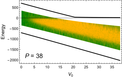
Figure 7: Energy-resolved r-statistic as a function of interaction strength, log-interaction, $P=38$. Both the energy and $r$ are averaged over 1001 consecutive states in the middle of the spectrum, and no fewer than 501 states near the edges. Orange regions correspond to Wigner-Dyson, while green to Poisson statistics. Thick black lines show the positions of the upper and lower boundaries of the spectrum.

Interestingly, the upper boundary that separates the Wigner-Dyson from Poisson level statistics approximately matches the extrapolation of the upper edge of the spectrum from high to low interactions, and vice versa. This is also where the fermionic and bosonic islands of scar states reside, see Fig. 5(b).

In addition to the QMBS near the top of the spectrum, there are other atypical states in the middle of the spectrum that are prominently present in Fig. 5(b) at intermediate couplings. These states have very large deviation from their typical neighbors in terms of the participation ratios. It is also notable that these atypical states form regular patterns in the energy-interaction strength plane, extending far beyond their parent domains. It thus appears that they also are a result of persistent level crossings, similar to the situation near the upper edge of the spectrum.

Similar physics may also arise in other models. Unfortunately, the most direct extension to non-chiral fermions makes the Hilbert space infinite in every total momentum sector $P$, making the numerical analysis more complex James et al. (2019). A rich variety of quantum spin models with and without quantum phase transitions may provide an alternative playground to test the connection between integrability and QMBS. In combination, these studies may shed light on the question of how general or particular QMBS are in many body systems, and their role in quantum dynamics and thermalization.

Note added. Shortly after our paper was submitted for publication, a related work Schindler et al. (2021) appeared that showed that in a chiral fermion system considered here, it is possible to non-trivially fine-tune interactions $V(q)$ in order to obtain exact fermionic QMBS at any overall interaction strength.