Effects of Non-linear Electrodynamics on Thermodynamics of Charged Black Hole

Abstract

This paper investigates thermodynamics, quasi-normal modes, thermal fluctuations and phase transitions of Reissner-Nordström black hole with the effects of non-linear electrodynamics. We first compute the expressions for Hawking temperature, entropy and heat capacity of this black hole and then obtain a relation between Davies’s point and quasi-normal modes with non-linear electrodynamics. We also observe the effects of logarithmic corrections on uncorrected thermodynamic quantities such as entropy, Hawking temperature, Helmholtz free energy, internal energy, Gibbs free energy, enthalpy and heat capacity. It is found that presence of non-linear electrodynamic parameter induces more instability in black holes of large radii. Finally, we analyze the phase transitions of Hawking temperature as well as heat capacity in terms of entropy for different values of charge ($q$), horizon radius ($r_{+}$) and coupling parameter ($\alpha$). We obtain that Hawking temperature changes its phase from positive to negative for increasing values of $q$ and $r_{+}$ while it shows opposite trend for higher values of $\alpha$. The heat capacity changes its phase from negative to positive for large values of charge, horizon radius and coupling parameter.

Keywords: Thermodynamics; Thermal fluctuations; Quasi-normal modes; Phase transitions.
PACS: 04.70.Dy; 04.70.-s; 05.70.Fh

1 Introduction

In general relativity, one of the most interesting subjects is the study of final outcomes of self-gravitating astronomical objects. Black hole (BH) is the completely collapsed structure of massive star which is defined as a thermodynamical object with infinite gravity such that nothing not even electromagnetic radiations such as light escape from it. There are some analogies between classical and BH laws of thermodynamics such as temperature is related to surface gravity of BH, energy has analogy with mass and entropy has resemblance with area of event horizon. These analogies motivated Bekenstein [1] to find out a relation between area and entropy of BH. In this regard, he found that entropy is proportional to area of the event horizon of BH and Hawking’s discovery of black body radiations further confirmed the validity of this relation. Consequently, it is impossible to obtain thermal equilibrium between BH and thermal radiations such as area of the event horizon of BH can never decrease. In this regard, the area-entropy relation proposed by Bekenstein needs to be corrected, leading to the concept of thermal fluctuations and holographic principle [2].

Quasi-normal modes (QNMs) are the perturbed solutions of linearized dynamical equations of BH characterized by complex eigenvalues where the real parts represent frequency oscillations and imaginary parts express damping modes. The origin of perturbations of BH is the pioneering work of Regge and Wheeler [3] which was further extended by Zerilli [4]. Vishveshwara [5] was the first to calculate QNMs by the scattering of gravitational waves from Schwarzschild BH. Leaver [6] formulated analytic representation of QNM wave-functions and also evaluated gravitational QNMs of both non-rotating and rotating BHs. Jing and Pan [7] studied the relationship between QNMs and second order phase transitions of the Reissner-Nordström (RN) BH. They found that both imaginary and real parts of QNM frequencies become oscillatory functions of charge and also contain thermodynamic information of BH.

Konoplya and Zhidenko [8] studied different aspects related to the perturbations of BHs, i.e., decoupling of variables in perturbed equations, anti-de Sitter (AdS) evaluation of QNMs, late-time tails, holographic superconductors and gravitational stability. Konoplya and Stuchlik [9] calculated analytical relation for gravitational QNMs in the eikonal limit and studied the null geodesics of asymptotically flat BH. Breton et al. [10] discussed QNMs as well as absorption cross-sections for the Born-Infeld-dS BHs and used Wentzel-Kramers-Brillouin approximation as well as null geodesics to evaluate QNMs of massless scalar fields. Ovgun and Jusufi [11] discussed the QNMs, stability, greybody factor and absorption cross section of $f(R)$ gravity minimally coupled to a cloud of strings in 2+1 dimensions. Ovgun et al. [12] formulated the QNMs for two types of BHs such as 4-dimensional dS and 5-dimensional Schwarzschild-AdS BHs by using feedforward neural network method and found that obtained results are similar to previous ones calculated from other methods.

Churilova [13] found analytical QNMs of BHs in different theories and added corrections due to deviations from Einstein theory. He also derived a general relation for analytical evaluation of the eikonal QNMs for asymptotically flat metrics with small deviations from the Schwarzschild geometry. Sakalli et al. [14] evaluated the QNMs and solution of Klein-Gordon equation in Born-Infeld dilaton spacetime with cosmic string. Wei and Liu [15] studied analytical relation between Davies point and QNMs for RN BH in the eikonal limit and concluded that QNMs can be obtained from null geodesics using the angular velocity as well as Lyapunov exponent of photon sphere.

Fluctuations in compact objects due to statistical perturbations are known as thermal fluctuations which has significant impact on the geometry of BH. It is believed that Hawking radiations reduce the size of BH which leads to increase its temperature. Faizal and Khalil [16] studied the effect of logarithmic corrections on thermodynamics of three BHs, i.e., RN, Kerr as well as charged AdS BHs and found that these BHs produce remnants in all cases. Pourhassan and Faizal [17] analyzed the effect of thermal fluctuations on thermodynamic quantities of a small singly spinning Kerr-AdS BH. They found that these fluctuations correct the entropy of BH by a logarithmic correction term and also noted that logarithmic corrections are very important for sufficiently small BHs.

Jawad and Shahzad [18] discussed the effects of thermal fluctuations on non-minimal regular BHs with cosmological constant and found that BHs are stable both locally as well as globally for large values of cosmological constant. Zhang [19] analyzed the effect of first order correction terms to the entropy of RN-AdS as well as Kerr-Newman-AdS BHs and concluded that corrected entropy only affects the thermodynamic potentials of small BHs. Pradhan [20] studied thermodynamics and thermal fluctuations for charged accelerating BHs and found that such BHs are stable as well as second order phase transitions occur in them.

Davies [21] developed thermodynamical theory of BHs and found that phase transition occurs in Kerr-Newman BHs. Hawking and Page [22] determined the presence of phase transition in Schwarzschild-AdS BH. Biswas and Chakraborty [23] investigated that whether phase transition is possible in Horava Lifshitz gravity under the consideration of classical and topological choices of BH thermodynamics. They concluded that phase transition occurs in Horava Lifshitz gravity from stable to unstable phase for increasing values of radius. Kubiznak and Mann [24] analyzed the first order small-large BHs phase transition in charged AdS BH which is analogous to liquid-gas phase transitions of fluids. Tharanath et al. [25] studied thermodynamical properties as well as phase transition of regular BHs and found that regular BHs undergo second order phase transition.

Chaturvedi et al. [26] investigated phase transition in the framework of thermodynamic geometry for charged AdS BH and found first order phase transition for fixed electric charge. Wei et al. [27] studied thermodynamics and found first order phase transition for charged AdS BHs in five-dimensions. Ovgun [28] studied the thermodynamics as well as phase transition of a specific charged AdS type BH in $f(R)$ gravity coupled with Yang-Mills field by considering cosmological constant as thermal pressure. Wei and Liu [29] discussed a relation between phase transition and null geodesics of charged AdS BH. Saleh et al. [30] examined thermodynamics as well as phase transition of Bardeen BH surrounded by quintessence and found that presence of quintessence induces phase transition in considered BH. Kuang et al. [31] evaluated thermal quantities of AdS non-linear electrodynamic BH. Bhatacharya et al. [32] provided a general criteria to get information and other various results with an extremal limit of BH spacetime. They also evaluated critical values of second order phase transition without considering any specific BH and showed that these values are in agreement with those of any specific BH cases.

Gonzalez et al. [33] studied thermodynamics and stability of charged BHs with non-linear electrodynamics and found that small BHs are stable locally. Balart and Vagenas [34] derived the solutions of many regular BHs with non-linear electrodynamics and verified that some of them show asymptotic behavior to RN BH. Dayyani [35] studied thermodynamical properties and phase transition of dilaton BH with non-linear electrodynamics and observed zeroth order phase transition. Yu and Gao [36] derived the exact solutions of RN BH with non-linear electrodynamics. Javed et al. [37] observed the effect of non-linear electrodynamics on weak field deflection angle of RN BH. Recently, Fauzi and Ramadhan [38] discussed thermodynamics of charged BHs with non-linear electrodynamics and verified the first law of BH thermodynamics.

In this paper, we study thermodynamical quantities, QNMs, thermal fluctuations and phase transition for RN BH with non-linear electrodynamic effects. The paper is outlined as follows. In section 2, we discuss thermodynamics as well as thermal stability for the considered BH by using heat capacity. Section 3 is devoted to examine the relation between QNMs and Davies point. In section 4, we study the effects of thermal fluctuations on uncorrected thermodynamical quantities and section 5 analyzes phase transitions in terms of entropy. In the last section, we conclude all the results.

2 Thermodynamics

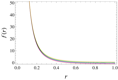
Figure 1: Plot of the metric function versus $r$ for $M=1=q$ with $\alpha=-0.4$(red), -0.2(blue), 0(black), 0.2(green) and 0.4(orange).

In this section, we discuss thermodynamics of RN BH with non-linear electrodynamic effects such as Hawking temperature and heat capacity. We also use derived expression of heat capacity to explore the thermal stable configuration of the system. The line element of considered BH is given as [37]

$$ds^{2}=f(r)dt^{2}-\frac{dr^{2}}{f(r)}-r^{2}d\theta^{2}-r^{2}\sin^{2}\theta d\phi^{2},$$ (1)

with

$$f(r)=1-\frac{2M}{r}+\frac{q^{2}}{r^{2}}+2\alpha q-\frac{\alpha^{2}r^{2}}{3},$$ (2)

$M$, $q$ and $\alpha$ represent mass of BH, charge and coupling constant, respectively. The line element (1) reduces to the RN BH when $\alpha=0,~{}q\neq 0$, Schwarzschild metric for $\alpha=0,~{}q=0$ and it becomes Schwarzschild BH with the effects of non-linear electrodynamics for $\alpha\neq 0,~{}q=0$. In Figure 1, the graphical analysis of metric function (2) shows the appearance of naked singularities for negative as well as positive values of coupling parameter. Setting $f(r_{+})=0$, the mass of BH in terms of $r_{+}$ can be obtained as

$$M=\frac{3q^{2}+6\alpha qr_{+}^{2}-\alpha^{2}r_{+}^{4}+3r_{+}^{2}}{6r_{+}}.$$ (3)

where $r_{+}$ is the horizon radius of BH. To obtain the expression for Hawking temperature, we first evaluate surface gravity of the BH

$$\kappa=-\frac{\left(q-\alpha r_{+}^{2}+r_{+}\right)(q-r_{+}(\alpha r_{+}+1))}{2r_{+}^{3}}.$$

Consequently, the Hawking temperature $(T=\frac{\kappa}{2\pi})$ is

$$T=-\frac{\left(q-\alpha r_{+}^{2}+r_{+}\right)(q-r_{+}(\alpha r_{+}+1))}{4\pi r_{+}^{3}}.$$ (4)

The graphical sketch of Hawking temperature versus $\alpha$ is shown in the left plot of Figure 2. It is found that Hawking temperature increases with the increasing values of coupling parameter throughout the considered domain.

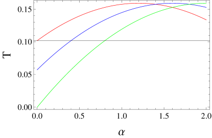
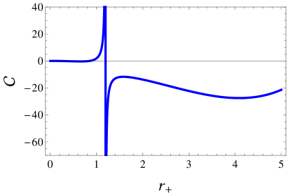
Figure 2: Plot of Hawking temperature (left) versus $\alpha$ for $r_{+}=0.5$ with $q=0.3$(red), 0.4(blue), 0.5(green) and plot of heat capacity (right) versus $r_{+}$ with $q=1$ and $\alpha=0.2$.

According to Bekenstein area-entropy relation, the entropy of BH can be evaluated as [39]

$$S=\int_{0}^{2\pi}\int_{0}^{\pi}\sqrt{g_{\theta\theta}g_{\phi\phi}}d\theta d\phi=\pi r_{+}^{2}.$$ (5)

In order to analyze the thermal stability of BH, heat capacity $(T\frac{\partial S}{\partial T})$ can be calculated as follows

$$C=\frac{\pi r_{+}^{2}\left(q-\alpha r_{+}^{2}+r_{+}\right)(q-r_{+}(\alpha r_{+}+1))}{-2q^{2}+2\alpha qr_{+}^{2}+r_{+}^{2}}.$$ (6)

It is noted that heat capacity of the considered system diverges at $r_{+}=1.2$ (right plot of Figure 2) and this divergent point of heat capacity is known as Davies point. The positive region before Davies point shows that BHs with small radii are stable while negative region after Davies point shows that BHs with large radii are unstable in the presence of $\alpha$.

Now we analyze the relationship between Davies point and QNMs. In this regard, we calculate the heat capacity in terms of mass $M$. For this purpose, the Hawking temperature in terms of $M$ is given as

$$T=\frac{3Mr_{+}-3q^{2}-\alpha^{2}r_{+}^{4}}{6\pi r_{+}^{3}}.$$ (7)

Consequently, the heat capacity becomes

$$C=\frac{2\pi r_{+}^{2}\left(-3Mr_{+}+3q^{2}+\alpha^{2}r_{+}^{4}\right)}{6Mr_{+}-9q^{2}+\alpha^{2}r_{+}^{4}}.$$ (8)

The divergence point of heat capacity can be calculated by considering the denominator of Eq.(8) equal to zero as

$$6Mr_{+}-9q^{2}+\alpha^{2}r_{+}^{4}=0.$$

Here, it is difficult to get divergence point of heat capacity because $q$ cannot be obtained explicitly in terms of $M$. In this regard, we plot heat capacity to get divergence point and to analyze its physical behavior.

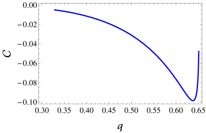
Figure 3: Heat capacity versus $q$ for $M=1$ and $\alpha=1.1$.

Figure 3 represents the graphical analysis of heat capacity in terms of $q$ and shows that considered BH is thermodynamically unstable. It is also noted that heat capacity diverges at $q=0.65$.

3 Null Geodesics and Quasi-normal Modes

This section is devoted to discuss the null geodesics and photon sphere radius for RN BH with non-linear electrodynamics. We use photon sphere radius to calculate angular velocity of the photon and Lyapunov exponent. We restrict ourselves to the equatorial plane ($\theta=0,\frac{\pi}{2}$) and the corresponding Lagrangian becomes [40]

$$2\mathcal{L}=\textit{f(r)}\dot{t}^{2}-\textit{f(r)}^{-1}\dot{r}^{2}-{r}^{2}\dot{\phi}^{2},$$ (9)

where $\phi$ represents angular coordinate. The components ($\mathcal{P}_{u}=g_{uv}\dot{x}^{v}=\frac{\partial\mathcal{L}}{\partial\dot{x}^{u}}$) of generalized momenta are given as

$$\mathcal{P}_{t} = f(r)\dot{t}=\bar{E}=constant,$$ (10)

$$\mathcal{P}_{r} = -{f(r)}^{-1}\dot{r},$$ (11)

$$\mathcal{P}_{\phi} = -{r}^{2}\dot{\phi}\equiv-l=constant,$$ (12)

where energy and angular momentum of the photon are represented by conservation constants $\bar{E}$ and $l$, respectively. Using Eqs.(10) and (12), $t$ and $\phi$-motions are evaluated as

$$\dot{t}={f(r)}^{-1}\bar{E},\quad\dot{\phi}=\frac{1}{{r}^{2}}l.$$

The corresponding Hamiltonian yields

$$2\mathcal{H}=-\dot{r}^{2}{f(r)}^{-1}+f(r)\dot{t}^{2}-{r}^{2}\dot{\phi}^{2}=\bar{E}\dot{t}-\dot{r}^{2}{f(r)}^{-1}-l\dot{\phi}=0,$$ (13)

which leads to

$$V_{\text{eff}}=-\dot{r}^{2},$$

where

$$V_{\text{eff}}=\frac{f(r)l^{2}-\bar{E}^{2}r^{2}}{r^{2}}.$$ (14)

This relation expresses that for positive $\dot{r}^{2}$, effective potential becomes negative which indicates that photon cannot escape from the region of negative potential. For large $l$ and small $r$, the photon will drive out before falling inside the BH while for large $r$ and small $l$, the photon will fall into the BH. However, there is another region at a distance equal to the radius of BH horizon where photon revolves around BH with zero radial velocity [40]. These circular orbits are unstable and are known as photon sphere.

For spherically symmetric metric, photon sphere can be determined by the following conditions

$$V_{\text{eff}}=0,\quad\frac{\partial V_{\text{eff}}}{\partial r}=0,\quad\frac{\partial^{2}V_{\text{eff}}}{\partial r^{2}}<0.$$ (15)

Photon sphere radius $(r_{ps})$ can be evaluated by using first condition of Eq.(15) while the third condition ensures about instability of photon sphere and associates with the QNMs of BH. By using Eq.(14) in the second condition, we obtain

$$f^{{}^{\prime}}(r_{ps})r_{ps}-2f(r_{ps})=0.$$ (16)

For the given metric function (2), it becomes

$$3Mr_{ps}=2q^{2}+r_{ps}^{2}+2qr_{ps}^{2}\alpha.$$

The photon sphere radius is given as

$$r_{ps}=\frac{3M+\sqrt{9M^{2}-8q^{2}-16q^{3}\alpha}}{2\left(1+2q\alpha\right)}.$$ (17)

This reduces to the photon sphere radius of RN BH for $\alpha=0$ [15]. In the eikonal limit $(l\gg 1)$, QNMs can be evaluated by using the property of the photon sphere [41]

$$w_{Q}=\Omega l-i|\lambda|\Big{(}\frac{2n+1}{2}\Big{)},$$ (18)

where the number of overtune of the perturbations and angular momentum of the photon are represented by $n$ and $l$, respectively. The angular velocity $\Omega$ and Lyapunov exponent $\lambda$ are two important quantities of the photon sphere. These are related to QNMs as

$$\Omega=\dot{\phi}\frac{1}{\dot{t}}\Big{|}_{r_{ps}}=\frac{\sqrt{f_{ps}}}{r_{ps}},\quad\lambda=\sqrt{\frac{-V_{\text{eff}}^{{}^{\prime\prime}}}{2\dot{t}^{2}}}\Big{|}_{r_{ps}}=\sqrt{\frac{(2f_{ps}-f_{ps}^{{}^{\prime\prime}}r_{ps}^{2})f_{ps}}{2r_{ps}^{2}}},$$ (19)

which yield

$$\Omega = \frac{\sqrt{1+\frac{q^{2}-2Mr_{ps}}{r_{ps}^{2}}+2q\alpha-\frac{r_{ps}^{2}\alpha^{2}}{3}}}{r_{ps}},$$

$$\lambda = \left(-\left(\left(-2q^{2}+r_{ps}^{2}+2qr_{ps}^{2}\alpha\right)\left(-3\left(q^{2}+r_{ps}\left(-2M+r_{ps}\right)\right)\right.\right.\right.$$

$$- \left.\left.\left.6qr_{ps}^{2}\alpha+r_{ps}^{4}\alpha^{2}\right)\right)\left(3r_{ps}^{6}\right)\right)^{\frac{1}{2}}.$$

The graphical behavior of angular velocity versus $q$ shows that there is no effect of coupling parameter on the angular velocity of photon for the considered values (Figure 4 (left)). It is also observed that angular velocity of photon is not defined before $q=0.65$ which is the Davies point of $\Omega$. However, the right plot shows that increasing rate of angular velocity and radius of photon sphere are inversely proportional to each other. It is interesting to mention here that the Davies point noted from Figures 3 and 4 are exactly the same. Figure 5 shows the graphical representation of lyapunov exponent versus $q$. It is observed that lyapunov exponent shows increasing behavior for increasing values of photon sphere radius and coupling parameters which indicate the increasing rate of modes of perturbation.

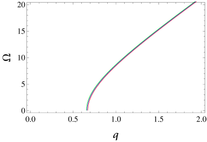
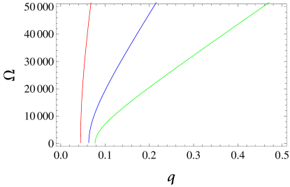
Figure 4: Plots of $\Omega$ versus $q$ for $M=1$, $r_{ps}=0.3$ and $\alpha=0.5$(red), 0.6(blue), 0.7(green) for the left plot and $M=\alpha=1$ with $r_{ps}=0.001$(red), 0.002(blue), 0.003(green) for the right plot.

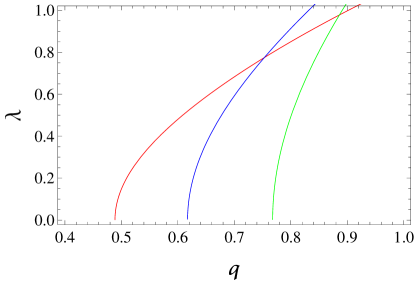
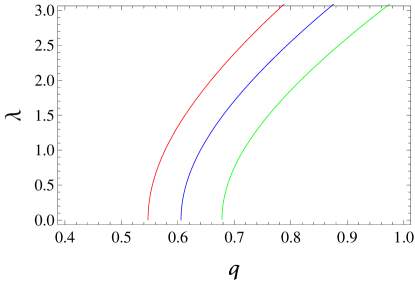
Figure 5: Plots of $\lambda$ versus $q$ for $M=1$, $r_{ps}=1.5$ with $\alpha=1$(red), 1.5(blue), 2(green) for the left plot and $M=1$, $\alpha=3$ with $r_{ps}=0.9$(red), 1(blue), 1.1(green) for the right plot.

4 Thermal Fluctuations

In this section, we investigate the effects of thermal fluctuations on thermodynamical potentials of RN BH with non-linear electrodynamics. We compute the corrected and uncorrected expressions of physical quantities. By using Eq.(2) and taking $f(r_{+})=0$, we have

$$3r_{+}^{2}-6r_{+}M+3q^{2}+6r_{+}q\alpha-\alpha^{2}r_{+}^{4}=0.$$ (20)

Consequently, the Hawking temperature turns out to be

$$T=\frac{3Mr_{+}-3q^{2}-\alpha^{2}r_{+}^{4}}{6\pi r_{+}^{3}}.$$

In order to evaluate corrected expression for entropy, we define the partition function as [20]

$$R(\xi)=\int_{0}^{\infty}\exp(-\xi E)\rho(E)dE,$$ (21)

where $\rho(E)$ and $E$ are the density of state and average energy, respectively. The inverse Laplace transform of the above partition function gives the density of state in the following form

$$\rho(E)=\frac{1}{2i\pi}\int_{-i\infty+\xi_{0}}^{i\infty+\xi_{0}}\exp(\xi E)R(\xi)d\xi=\frac{1}{2i\pi}\int_{-i\infty+\xi_{0}}^{i\infty+\xi_{0}}\exp(\tilde{S}(\xi))d\xi,$$ (22)

where $\tilde{S}(\xi)=\beta E+\ln Z(\xi)$ with $\xi>0$ is referred to as exact expression for entropy of the BH and has dependence on Hawking temperature. Using Taylor series expansion, we have

$$\tilde{S}(\xi)=S+\frac{1}{2}(\xi-\xi_{0})^{2}\frac{\partial^{2}\tilde{S}(\xi)}{\partial\xi^{2}}\Big{|}_{\xi=\xi_{0}}+O(\xi-\xi_{o})^{2}.$$ (23)

The equilibrium entropy $S$ satisfies the relations $\frac{\partial S}{\partial\xi}=0$ and $\frac{\partial^{2}S}{\partial\xi^{2}}>0$. By using Eq.(23) in (22), we obtain

$$\rho(E)=\frac{1}{2\pi i}\exp(S)\int d\xi\exp\Big{(}\frac{1}{2}(\xi-\xi_{0})^{2}\frac{\partial^{2}\tilde{S}(\xi)}{\partial\xi^{2}}\Big{)}.$$ (24)

Further, it can be written as [42]

$$\rho(E)=\frac{1}{\sqrt{2\pi}}\exp(S)\Big{(}\Big{(}\frac{\partial^{2}\tilde{S}(\xi)}{\partial\xi^{2}}\Big{)}\Big{|}_{\xi=\xi_{0}}\Big{)}^{-\frac{1}{2}},$$ (25)

which yields

$$\tilde{S}=S-\frac{1}{2}\ln(ST^{2})+\frac{\eta}{S}.$$ (26)

Without loss of generality, we can use a more general parameter $\gamma$ except the factor $\frac{1}{2}$ which increases the effect of correction terms on the entropy of BH. In this context, the corrected entropy can be written as [43]

$$\tilde{S}=S-\gamma\ln(ST^{2})+\frac{\eta}{S}.$$ (27)

For different values of correction parameters $\gamma$ and $\eta$, we obtain

• For $\eta,~{}\gamma\rightarrow 0$, we have the uncorrected entropy of BH.

• When $\eta\rightarrow 0,~{}\gamma\rightarrow 1$, this provides simple logarithmic corrections.

• When $\eta\rightarrow 1,~{}\gamma\rightarrow 0$, we obtain second order correction terms which are inversely proportional to the uncorrected entropy of the BH.

• For $\eta,~{}\gamma\rightarrow 1$, we obtain correction terms of higher orders.

In the following, we only consider the second case ($\eta\rightarrow 0,\gamma\rightarrow 1$). The second term in Eq.(27) is logarithmic which leads to the corrections in entropy. The perturbed expression of entropy can be obtained by using Eqs.(5) and (7) in (27) as

$$\tilde{S}=\pi r_{+}^{2}-2\gamma\ln\left(3Mr_{+}-3q^{2}-\alpha^{2}r_{+}^{4}\right)+\gamma\ln\left(36\pi r_{+}^{4}\right).$$ (28)

Figure 6 (left plots) represents the graphical behavior of corrected entropy in terms of horizon radius for different values of $\alpha$, $\gamma$ and $q$, respectively. It is noted that corrected entropy remains positive for considered values of $\alpha$, $\gamma$ as well as $q$ and hence satisfies the second law of thermodynamics. The first and third plots represent that thermal fluctuations and charge only affect the entropy of BHs negligibly for small radii while for large radii it remains in equilibrium position. However, the parameter $\alpha$ equally affects the entropy of both BHs with small as well as large radii (2nd plot).

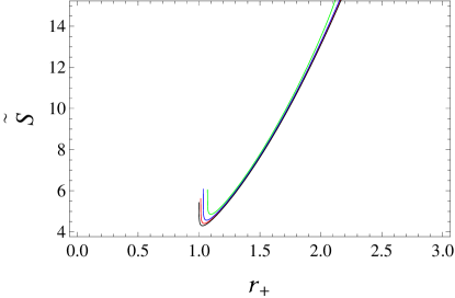
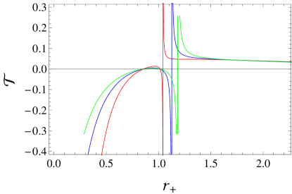
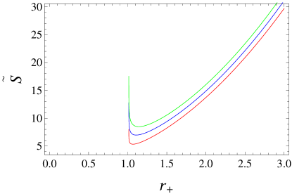
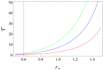
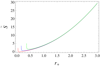
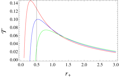
Figure 6: Corrected entropy (left 3 plots) versus $r_{+}$ for $M=q=1$. We take $\gamma=0.1$, with $\alpha=0$(black), 0.2(red), 0.3(blue), 0.4(green) for the 1st plot, $\alpha=0.2$ with $\gamma=0.2$(red), 0.4(blue), 0.6(green) for the 2nd plot and $M=1$, $\alpha=\gamma=0.2$ with $q=0.2$(red), 0.4(blue), 0.6(green) for the 3rd plot. Corrected Hawking temperature versus $r_{+}$ with $M=q=1$, $\alpha=0.2$ with $\gamma=0.1$(red), 0.5(blue), 0.9(green) for the 1st plot, $\gamma=5$ with $\alpha=10$(red), 15(blue), 20(green) for the 2nd plot and $M=1$, $\alpha=\gamma=0.2$ with $q=0.1$(red), 0.3(blue), 0.5(green) for the 3rd plot.

The modified first law of BH thermodynamics under thermal fluctuations can be written as [18]

$$dM = \mathcal{T}dS+\varphi dq+\Pi d\alpha,,$$ (29)

where $\mathcal{T}$ and $\varphi$ are corrected Hawking temperature and electric potential, respectively. Here, we consider $\alpha$ as a new thermodynamic variable and $\Pi$ is the corresponding conjugate quantity. These potential functions can be obtained from the relations

$$\mathcal{T}=\Big{(}\frac{\partial M}{\partial\tilde{S}}\Big{)}_{q,\alpha},\quad\varphi=\Big{(}\frac{\partial M}{\partial q}\Big{)}_{T,\alpha},\quad\Pi=\Big{(}\frac{\partial M}{\partial\alpha}\Big{)}_{T,q}$$

which yield

$$\mathcal{T} = \left(1-\frac{\left(q-\alpha r_{+}^{2}\right)^{2}}{r_{+}^{2}}\right)\left(2\left(\frac{6\gamma M-8\alpha^{2}\gamma r_{+}^{3}}{-3Mr_{+}+3q^{2}+\alpha^{2}r_{+}^{4}}+\frac{4\gamma}{r_{+}}+2\pi r_{+}\right)\right)^{-1},$$

$$\varphi = \frac{3}{2}\left(1-\frac{\left(q-\alpha r_{+}^{2}\right)^{2}}{r_{+}^{2}}\right)\left(\frac{\sqrt{3}\left(3M+8\alpha^{2}r_{+}^{3}-3r_{+}\right)}{\sqrt{r_{+}\left(6M+4\alpha^{2}r_{+}^{3}-3r_{+}\right)}}-6\alpha r_{+}\right)^{-1},$$

$$\Pi = \frac{-6q\sqrt{r_{+}^{4}\left(-2Mr_{+}+4q^{2}+r_{+}^{2}\right)}+\sqrt{3}r_{+}^{3}(3M-r_{+})-8\sqrt{3}q^{2}r_{+}^{2}}{r_{+}^{3}\sqrt{r_{+}^{4}\left(r_{+}(r_{+}-2M)+4q^{2}\right)}}.$$

The modified first law of BH gets satisfied on substitution of above expressions in Eq.(29) indicating that the presence of thermal fluctuations increases the validity of first law of BH thermodynamics.

The graphical analysis of corrected Hawking temperature versus $r_{+}$ is shown in Figure 6 (right plots). It is observed that temperature of BHs with small radii are affected by thermal fluctuations while the region after the divergence point shows that BHs of large radii are unaffected (first plot). It is also observed that critical radius of BH increases by increasing the values of correction parameter. The second plot shows the profile of corrected Hawking temperature for different values of coupling parameter. We note that the corrected Hawking temperature increases monotonically with respect to horizon radius. However, with increasing values of charge, temperature firstly increases and then shows decreasing behavior for large radii (3rd plot).

Now, we use the expressions of corrected entropy as well as Hawking temperature to explore thermodynamical equations of state. In this regard, the Helmholtz free energy can be obtained by using the relation

$$F=-\int\tilde{S}dT.$$ (30)

Inserting the expressions of $\tilde{S}$ and $T$, the Helmholtz free energy is given as

$$F = \left(3\gamma\left(-3Mr_{+}+4q^{2}+4\alpha^{2}r_{+}^{4}\right)+3\gamma\left(-3Mr_{+}+3q^{2}+\alpha^{2}r_{+}^{4}\right)\right.$$

$$\times \left.\left(\ln\left(36\pi r_{+}^{4}\right)-2\ln\left(3Mr_{+}-3q^{2}-\alpha^{2}r_{+}^{4}\right)\right)+18\pi Mr_{+}^{3}\ln(r_{+})\right.$$

$$+ \left.\pi\left(27q^{2}r_{+}^{2}+\alpha^{2}r_{+}^{6}\right)\right)\left(18\pi r_{+}^{3}\right)^{-1}.$$

The graphical representation of Helmholtz free energy versus $r_{+}$ is shown in Figure 7 (left plots). It is observed that the Helmholtz free energy remains positive throughout the considered domain for increasing values of $\gamma$ and $\alpha$ (1st and 2nd plots). Thermal fluctuations affect the Helmholtz free energy of BHs with small radii more as compared to the BHs of large radii for increasing values of $\gamma$ while for different values of $\alpha$, it shows opposite trend. However, the third plot represents that Helmholtz free energy increases from negative to positive values with increasing values of $q$.

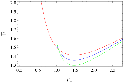
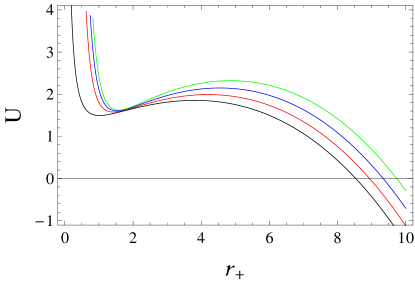
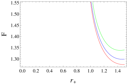
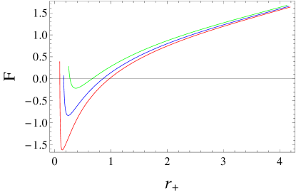
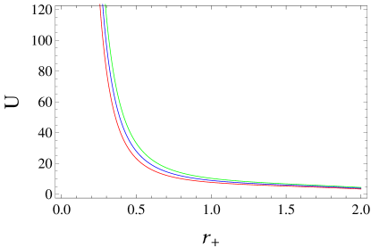
Figure 7: Helmholtz free energy versus $r_{+}$ for $M=q=1$. We take $\alpha=0.2$ with $\gamma=0$(red), 0.5(blue), 1(green) for the 1st plot, $\gamma=1$ with $\alpha=0.1$(red), 0.2(blue), 0.3(green) for the 2nd plot and $M=1$, $\alpha=\gamma=0.2$ with $q=0.3$(red), 0.4(blue). 0.5(green) for the 3rd plot. Internal energy versus $r_{+}$ for $M=g=1$. We take $\alpha=0.2$ with $\gamma=0$(black), 5(red), 10(blue), 15(green) for the 1st plot, $\gamma=0.1$ with $\alpha=0$(black), 0.01(red), 0.04(blue), 0.07(green) for the 2nd plot and $M=1$, $\alpha=\gamma=2$ with $q=2.1$(red), 2.3(blue), 2.5(green) for the 3rd plot.

The internal energy of the considered system can be evaluated by the identity, $U=\tilde{S}T+F$ [41] as

$$U = \left(3\gamma\left(-3Mr_{+}+4q^{2}+4\alpha^{2}r_{+}^{4}\right)+\pi r_{+}^{2}\left(9Mr_{+}+18q^{2}-2\alpha^{2}r_{+}^{4}\right)\right.$$ (31)

$$+ \left.18\pi Mr_{+}^{3}\ln(r_{+})\right)\left(18\pi r_{+}^{3}\right)^{-1}.$$

Figure 7 (right plots) shows the graphical analysis of internal energy versus $r_{+}$ for different values of the correction and coupling parameters. It is noted that the internal energy fluctuates with the increasing values of correction parameter and becomes negative for large values of horizon radius (1st plot). The left plot shows that internal energy decreases and remains unaffected by thermal fluctuations for small values of $r_{+}$ while it shows increasing behavior for large values of $\alpha$. However, third plot represents that BHs with large values of charge have less internal energy and vice versa.

The volume of the BH can be given as [43]

$$V=\frac{4}{3}\pi r_{+}^{3}.$$ (32)

The pressure of the BH can be calculated by the relation

$$P=-\frac{dF}{dV}=-\frac{dF}{dr_{+}}\frac{dr_{+}}{dV},$$ (33)

hence

$$P = -\left(\left(6Mr_{+}-9q^{2}+\alpha^{2}r_{+}^{4}\right)\left(-2\gamma\ln\left(3Mr_{+}-3q^{2}-\alpha^{2}r_{+}^{4}\right)\right.\right.$$

$$+ \left.\left.\gamma\ln\left(36\pi r_{+}^{4}\right)+\pi r_{+}^{2}\right)\right)\left(24\pi^{2}r_{+}^{6}\right)^{-1}.$$

The graphical behavior of pressure versus $r_{+}$ for different values of $\gamma$, $\alpha$ and $q$ is shown in Figure 8 (left plots). It is observed that for $\gamma=0$ (no thermal fluctuations) pressure firstly increases for small radii and becomes negative and it increases continuously for large radii but remains negative throughout the considered domain. However, in the presence of thermal fluctuations, it is affected significantly and is not defined for $r_{+}>3.8$ (1st plot). The second plot also shows that pressure is decreasing and becomes negative for increasing values of $\alpha$ while it becomes singular for $\alpha>0.556$. For increasing values of charge pressure, it also increases and coincides with equilibrium condition but remains negative for the considered domain.

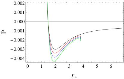
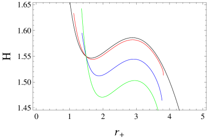
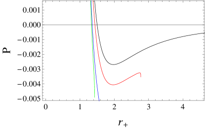
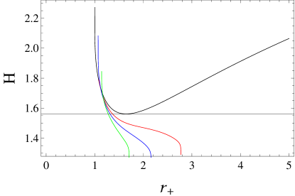
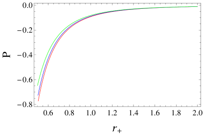
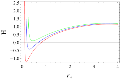
Figure 8: Pressure (left 3 plots) versus $r_{+}$ with $M=q=1$. We take $\alpha=0.2$ with $\gamma=0$(black), 0.3(red), 0.6(blue), 0.9(green) for the 1st plot, $\gamma=0.2$ with $\alpha=0$(black), 0.3(red), 0.5(blue), 0.556(green) for the 2nd plot and $M=1$, $\alpha=\gamma=0.2$ with $q=0.1$(red), 0.2(blue), 0.3(green) for the 3rd plot. Enthalpy (right 3 plots) versus $r_{+}$ for $M=q=1$. We take $\alpha=0.2$ with $\gamma=0$(black), 0.1(red), 1(blue), 2(green) for the 1st plot, $\gamma=0.5$ with $\alpha=0$(black), 0.3(red), 0.4(blue), 0.5(green) for the 2nd plot and and $M=1$, $\alpha=\gamma=0.2$ with $q=0.3$(red), 0.4(blue), 0.5(green) for the 3rd plot.

The enthalpy $(H=U+VP)$ of the system can be evaluated as

$$H = \left(3\gamma\left(-3Mr_{+}+4q^{2}+4\alpha^{2}r_{+}^{4}\right)+\left(-6Mr_{+}+9q^{2}-\alpha^{2}r_{+}^{4}\right)\right.$$

$$\times \left.\left(-2\gamma\ln\left(3Mr_{+}-3q^{2}-\alpha^{2}r_{+}^{4}\right)+\gamma\ln\left(36\pi r_{+}^{4}\right)+\pi r_{+}^{2}\right)\right.$$

$$+ \left.\pi r_{+}^{2}\left(9Mr_{+}+18q^{2}-2\alpha^{2}r_{+}^{4}\right)+18\pi Mr_{+}^{3}\ln(r_{+})\right)\left(18\pi r_{+}^{3}\right)^{-1}.$$

Figure 8 (right plots) shows that enthalpy of the system remains positive throughout the considered domain for different values of $\gamma$ and $\alpha$. It is observed that for both with and without thermal fluctuations, enthalpy of the considered system fluctuates in terms of $r_{+}$ (1st plot). However, the second plot shows that it decreases for small radii and then increases gradually for BHs of large radii in the absence of non-linear electrodynamic effects. For non-zero $\alpha$, enthalpy of the system decreases gradually and is affected only for BHs of large radii. However, for increasing values of charge enthalpy of the considered system also increases and gets equilibrium position for large radii (3rd plot).

The Gibbs free energy $(G=-\tilde{S}T+H)$ can be obtained as

$$G = \left(3\gamma\left(-3Mr_{+}+4q^{2}+4\alpha^{2}r_{+}^{4}\right)+\gamma\left(-15Mr_{+}+18q^{2}+2\alpha^{2}r_{+}^{4}\right)\right.$$

$$\times \left.\left(\ln\left(36\pi r_{+}^{4}\right)-2\ln\left(3Mr_{+}-3q^{2}-\alpha^{2}r_{+}^{4}\right)\right)-6\pi r_{+}^{2}\left(Mr_{+}-6q^{2}\right)\right.$$

$$+ \left.18\pi Mr_{+}^{3}\ln(r_{+})\right)\left(18\pi r_{+}^{3}\right)^{-1}.$$

Figure 9 (left plots) indicates the graphical behavior of Gibbs free energy in terms of $r_{+}$ for different values of $\gamma$, $\alpha$ and $q$. For $\gamma=0$ (no thermal fluctuations), Gibbs free enrgy firstly decreases for small values of $r_{+}$ but remains positive and increases for large values of $r_{+}$. The presence of thermal fluctuations affects the Gibbs free energy with both small as well as large radii and ultimately becomes undefined for $r_{+}>3.8$ (1st plot). However, the second plot shows that for $\alpha=0$, the Gibbs free energy firstly decreases and becomes negative for BHs of small radii and then becomes positive by increasing for BHs of large radii. In the presence of non-linear electrodynamics, the Gibbs free energy of BHs with large radii are affected notably and BHs of small radii are affected negligibly. However, for different values of charge, the Gibbs free energy shows increasing behavior and coincides for large values of horizon radius.

We investigate thermal stability of RN BH with non-linear electrodynamic effects by means of specific heat $(C_{S}=\frac{dU}{dT})$ [41] given as

$$C_{S} = -\frac{2\left(\gamma\left(3Mr_{+}-6q^{2}+2\alpha^{2}r_{+}^{4}\right)-\pi r_{+}^{2}\left(-3Mr_{+}+3q^{2}+\alpha^{2}r_{+}^{4}\right)\right)}{6Mr_{+}-9q^{2}+\alpha^{2}r_{+}^{4}}.$$

Figure 9 (right plots) shows the graphical analysis of corrected heat capacity versus $r_{+}$. For different values of $\gamma$, the first plot shows that corrected heat capacity diverges at $r_{+}=1.47$ which is the Davies point. The positive region before the Davies point shows that BHs with small radii are stable under the effect of thermal fluctuations while the negative region after Davies point shows that BHs with large radii are unstable. However, for increasing values of coupling parameter, critical radius of RN BH with non-linear electrodynamics also increases (2nd plot). We note that BHs with small radii are unstable while BHs with large radii are stable for different values of $\alpha$. However, for different values of charge, only the divergence point of corrected heat capacity changes while before and after the Davies points, it remains in equilibrium condition (3rd plot).

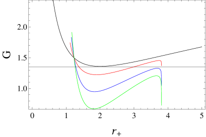
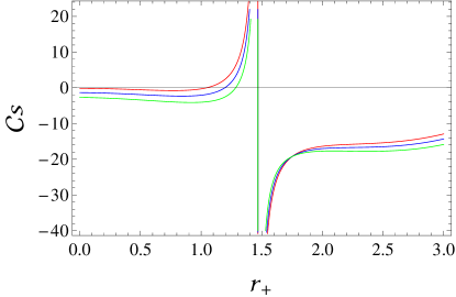
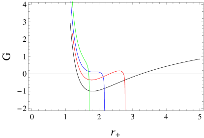
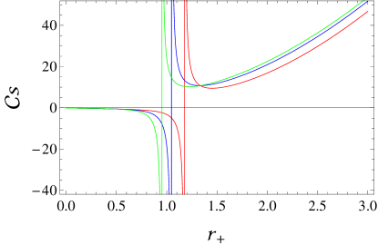
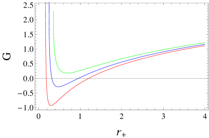
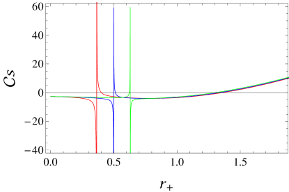
Figure 9: Gibbs free energy (left 3 plots) versus $r_{+}$ with $M=q=1$. We take $\alpha=0.2$ with $\gamma=0$ (black), 1(red), 3(blue), 5(green) for the 1st plot, $\gamma=15$ with $\alpha=0$(black), 0.3(red), 0.4(blue), 0.4(green) for the 2nd plot and $M=1$, $\alpha=\gamma=0.2$ with $q=0.4$(red), 0.5(blue), 0.6(green) for the 3rd plot. Corrected heat capacity (right 3 plots) versus $r_{+}$ for $M=q=1$. We take $\alpha=0.2$ with $\gamma=0.1$(red), 1(blue), 2(green) for the 1st plot, $\gamma=0.1$ with $\alpha=1$(red), 1.5(blue), 2(green) for the 2nd plot and $M=1$, $\alpha=\gamma=2$ with $q=0.5$(red), 0.6(blue), 0.7(green) for the 3rd plot.

We can also analyze the stability of a BH by using trace of Hessian matrix. The Hessian matrix contains the partial derivatives of Helmholtz free energy with respect to Hawking temperature as well as chemical potential $\upsilon=\Big{(}\frac{\partial M}{\partial q}\Big{)}_{r_{+}}$. The Hessian matrix is given as [17]

$$H=\left(\begin{array}[]{cc}H_{ii}&H_{ij}\\ H_{ji}&H_{jj}\\ \end{array}\right)=\left(\begin{array}[]{cc}\frac{\partial^{2}F}{\partial T^{2}}&\frac{\partial^{2}F}{\partial T\partial\upsilon}\\ \frac{\partial^{2}F}{\partial\upsilon\partial T}&\frac{\partial^{2}F}{\partial\upsilon^{2}}\\ \end{array}\right),$$

with $i\neq j$, and

$$H_{ii}=\frac{\partial^{2}F}{\partial T^{2}},\quad H_{ij}=\frac{\partial^{2}F}{\partial T\partial\upsilon},\quad H_{ji}=\frac{\partial^{2}F}{\partial\upsilon\partial T},\quad H_{jj}=\frac{\partial^{2}F}{\partial\upsilon^{2}}.$$

It is noted that $H_{ii}H_{jj}=H_{ij}H_{ji}$, which impies that one of the eigenvalues of Hessian matrix is zero. Therefore, to determine the stability of the considered geometry, we use trace of the Hessian matrix as

$$Tr(H)=H_{ii}+H_{jj},$$ (34)

where

$$H_{ii} = -\left(6\pi r_{+}^{4}\left(\frac{2\gamma\left(3Mr_{+}-6q^{2}+2\alpha^{2}r_{+}^{4}\right)}{r_{+}\left(-3Mr_{+}+3q^{2}+\alpha^{2}r_{+}^{4}\right)}-2\pi r_{+}\right)\right)$$

$$\times \left(6Mr_{+}-9q^{2}+\alpha^{2}r_{+}^{4}\right)^{-1},$$

$$H_{jj} = \left(\frac{2\gamma\left(q+\alpha r_{+}^{2}\right)\left(-3Mr_{+}+6q^{2}-2\alpha^{2}r_{+}^{4}\right)\left(-6Mr_{+}+9q^{2}-\alpha^{2}r_{+}^{4}\right)}{3Mr_{+}-3q^{2}-\alpha^{2}r_{+}^{4}}\right.$$

$$+ \left.\pi\left(3\alpha r_{+}^{4}\left(9q^{2}-4Mr_{+}\right)+9q^{3}r_{+}^{2}+3\alpha^{2}qr_{+}^{6}+\alpha^{3}r_{+}^{8}\right)+\gamma\left(-12Mqr_{+}\right.\right.$$

$$- \left.\left.24\alpha Mr_{+}^{3}+27q^{3}+45\alpha q^{2}r_{+}^{2}+\alpha^{2}qr_{+}^{4}-\alpha^{3}r_{+}^{6}\right)\left(\ln\left(36\pi r_{+}^{4}\right)\right.\right.$$

$$- \left.\left.2\ln\left(3Mr_{+}-3q^{2}-\alpha^{2}r_{+}^{4}\right)\right)\right)\left(6\pi r_{+}^{3}\left(q+\alpha r_{+}^{2}\right)^{3}\right)^{-1},$$

and we obtain

$$Tr = \left(\frac{2\gamma\left(q+\alpha r_{+}^{2}\right)\left(-3Mr_{+}+6q^{2}-2\alpha^{2}r_{+}^{4}\right)\left(-6Mr_{+}+9q^{2}-\alpha^{2}r_{+}^{4}\right)}{3Mr_{+}-3q^{2}-\alpha^{2}r_{+}^{4}}\right.$$

$$+ \left.\pi\left(3\alpha r_{+}^{4}\left(9q^{2}-4Mr_{+}\right)+9q^{3}r_{+}^{2}+3\alpha^{2}qr_{+}^{6}+\alpha^{3}r_{+}^{8}\right)+\gamma\left(-12Mqr_{+}\right.\right.$$

$$- \left.\left.24\alpha Mr_{+}^{3}+27q^{3}+45\alpha q^{2}r_{+}^{2}+\alpha^{2}qr_{+}^{4}-\alpha^{3}r_{+}^{6}\right)\left(\ln\left(36\pi r_{+}^{4}\right)\right.\right.$$

$$- \left.\left.2\ln\left(3Mr_{+}-3q^{2}-\alpha^{2}r_{+}^{4}\right)\right)\right)\left(6\pi r_{+}^{3}\left(q+\alpha r_{+}^{2}\right)^{3}\right)^{-1}-\left(6\pi r_{+}^{4}\right.$$

$$\times \left.\left(\frac{2\gamma\left(3Mr_{+}-6q^{2}+2\alpha^{2}r_{+}^{4}\right)}{r_{+}\left(-3Mr_{+}+3q^{2}+\alpha^{2}r_{+}^{4}\right)}-2\pi r_{+}\right)\right)\left(6Mr_{+}-9q^{2}+\alpha^{2}r_{+}^{4}\right)^{-1}.$$

A thermodynamical system is said to be stable if $Tr(H)\geq 0$ [44]. Figure 10 shows the graphical analysis of Hessian trace in terms of $r_{+}$ for different values of correction parameter, coupling parameter and charge. It is observed that BHs with small radii are unstable while BHs of large radii are stable for considered parameters which is same as noticed in the graphical analysis of corrected heat capacity (Figure 9).

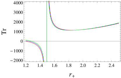
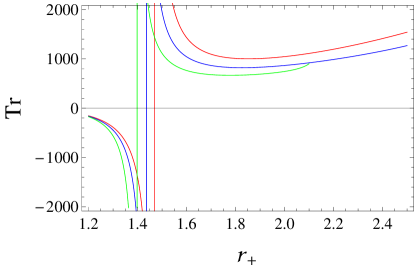
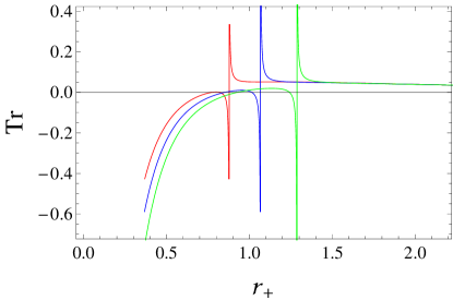
Figure 10: Hessian trace versus $r_{+}$ for $M=q=1$. We take $\alpha=0.1$ with $\gamma=1$(red), 1.5(blue), 2(green) for the left plot, $\gamma=0.1$ with $\alpha=0.2$(red), 0.3(blue) and 0.4(green) for the right plot and $M=1$, $\alpha=\gamma=0.2$ with $q=0.9$(red), 1(blue), 1.1(green) for the lower plot

.

5 Phase Transitions

Here we examine the phase transitions of Hawking temperature as well as heat capacity of RN BH with non-linear electrodynamic effects in terms of entropy. The Hawking temperature evaluated in Eq.(4) can be written in the form of entropy as

$$T=-\frac{\left(q-\alpha r_{+}^{2}+r_{+}\right)(q-r_{+}(\alpha r_{+}+1))}{4r_{+}S}.$$

Figure 11 (left plots) represents the phase transitions of Hawking temperature in terms of $S$ for different values of $q$, $r_{+}$ and $\alpha$, respectively. It is noted that the Hawking temperature changes its phase from positive to negative for increasing values of $q$ and $r_{+}$, respectively (1st and 2nd plot). However, for increasing values of non-linear electrodynamic parameter, the Hawking temperature changes its phase from negative to positive (3rd plot). The expression of heat capacity for RN BH with non-linear electrodynamic effects in terms of entropy can be obtained from Eq.(6) as

$$C=\frac{S\left(q-\alpha r_{+}^{2}+r_{+}\right)(q-r_{+}(\alpha r_{+}+1))}{-2q^{2}+2\alpha qr_{+}^{2}+r_{+}^{2}}.$$

The phase transitions of heat capacity versus entropy is shown in Figure 11 (right plots) for different values of $q$, $r_{+}$ and $\alpha$, respectively. It is noted that the right plots of Figure 11 show that heat capacity of the considered BH changes its phase from negative to positive for the increasing values of $q$, $r_{+}$ and $\alpha$. It is also observed that considered system is unstable for small values of considered parameters while it shows stable behavior for large values of $q$, $r_{+}$ and $\alpha$.

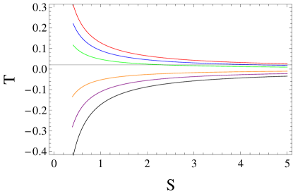
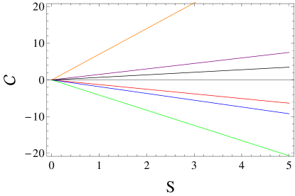
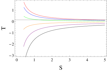
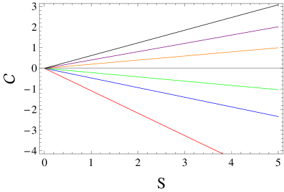
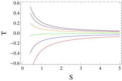
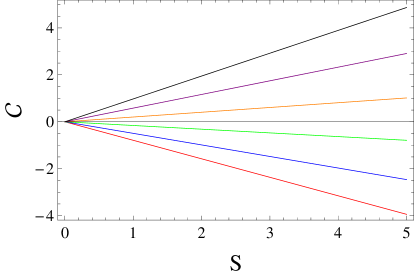
Figure 11: Hawking temperature (left 3 plots) versus $S$ for $\alpha=1$, $r_{+}=1$. We take $q=1.7$(red), 1.8(blue), 1.9(green), 2.1(orange), 2.2(purple), 2.3(black) for the 1st plot, $\alpha=1$, $q=1$ with $r_{+}=0.4$(red), 0.5(blue), 0.6(green), 0.7(orange), 0.8(purple), 0.9(black) for the 2nd plot and $r_{+}=3$, $q=1$ with $\alpha=0.2$(red), 0.3(blue), 0.4(green), 0.5(orange), 0.6(purple), 0.7(black) for the 3rd plot. Heat capacity (right 3 plots) versus $S$ with $r_{+}=1$, $\alpha=1$. We take $q=1.1$(red), 1.2(blue), 1.3(green), 1.4(orange), 1.5(purple), 1.6(black) for the 1st plot, $\alpha=2$, $q=1$ with $r_{+}=0.7$(red), 0.8(blue), 0.9(green), 1.1(orange), 1.2(purple), 1.3(black) for the 2nd plot and $r_{+}=3$, $q=1$, $\alpha=0.2$(red), 0.3(blue), 0.4(green), 0.5(orange), 0.6(purple), 0.7(black) for the 3rd plot.

6 Concluding Remarks

In this paper, we have discussed thermodynamical quantities for RN BH with non-linear electrodynamic effects. We have then derived the relationship between Davies point and QNMs as well as examined the effects of thermal fluctuations on uncorrected thermodynamical quantities and then compared both corrected as well as uncorrected quantities graphically. We have also analyzed the phase transitions of heat capacity and Hawking temperature.

Firstly, we have computed the Hawking temperature by means of surface gravity with the relation $(T=\frac{\kappa}{2\pi})$ and then heat capacity for the considered BH. The graphical analysis of heat capacity shows that heat capacity diverges at $r_{+}=1.2$ (Figure 2). It is also found that BHs with small radii are stable in the presence of non-linear electrodynamic effects while BHs with large radii are unstable. Secondly, we have discussed the null geodesics and QNMs for which we have evaluated the real part as angular velocity and imaginary part as Lyapunov exponent of QNMs. It is observed that angular velocity of photon remains unaffected by the effect of coupling parameter while lyapunov exponent shows increases behavior and significantly affected by coupling parameter. The interesting fact is that the Davies point evaluated from plots of heat capacity (Figure 3) and angular velocity (Figure 4) are exactly the same.

Further, we have obtained the corrected expression for entropy by considering logarithmic corrections of first order and then used it to calculate the modified results of thermodynamical potentials. It is found that corrected entropy remains positive as well as increasing monotonically but remains unaffected for increasing values of correction parameter. However, for increasing values of non-linear electrodynamics parameter, the corrected entropy of small as well as large BHs have similar behavior. The corrected Hawking temperature changes its behavior from negative to positive for increasing values of correction parameter and coincides with the equilibrium condition for large values of $r_{+}$. However, it becomes positive valued function as well as increases gradually for higher values of $\alpha$ and large BHs are affected more by $\alpha$ as compared to small ones.

The Helmholtz free energy shows similar behavior in the presence as well as absence of correction parameter but logarithmic corrections affect small BHs more as compared to large ones. However, for increasing values of $\alpha$, Helmholtz free energy shows decreasing behavior but it affects BHs with large radii more as compared to BHs of small radii. The internal energy fluctuates in both absence as well as presence of $\gamma$ and affects both large as well as small BHs negligibly. The internal energy of BHs with radii from $r_{+}=0$ to 4 remains unaffected for increasing values of $\alpha$ and only affects BHs with radii $r_{+}>4$.

The enthalpy of the considered system also fluctuates with increasing values of $\gamma$ and decreases continuously for large event horizon. However, this shows decreasing behavior for small values of $r_{+}$ and increases with large values of $r_{+}$ for $\alpha=0$ but shows only decreasing trend in the presence of $\alpha$. It is also noted that the increasing values of both correction and coupling parameters only affect BHs with large radii. We have found that the corrected heat capacity diverges at $r_{+}=1.47$ and also observed that BHs with radii greater than 1.47 are unstable under the effect of thermal fluctuations. Black holes with small radii are unstable while BHs with large radii are stable for considered values of coupling parameter. It is also noted that critical radius of BH increases with the increasing values of $\alpha$.

Finally, we have investigated the phase transitions of Hawking temperature as well as heat capacity in terms of entropy for the considered BH. It is found that Hawking temperature changes its phase from positive to negative for increasing values of both charge and horizon radius. This shows that BHs with small charge and radii are more hotter than the BHs with large charge and radii while it shows opposite behavior for increasing values of coupling parameter. The heat capacity changes its phase from negative to positive for increasing values of considered parameters which shows that BHs with small values of $q$, $r_{+}$ and $\alpha$ are unstable while BHs with large values are stable throughout the considered domain. We would like to mention here that all our results reduce to the RN BH for $\alpha=0$ [16].

References

- [1] Bekenstein, D.: Phys. Rev. D 7(1973)2333.
- [2] Easther, R. and Lowe, D.: Phys. Rev. Lett. 82(1999)4967.
- [3] Regge, T. and Wheeler, J.A.: Phys. Rev. 108(1957)1063.
- [4] Zerilli, F.J.: Phys. Rev. D 2(1970)2141.
- [5] Vishveshwara, C.V.: Nature 227(1970)936.
- [6] Leaver, E.W.: Proc. R. Soc. Lond. 402(1985)285.
- [7] Jing, J. and Pan, Q.: Phys. Lett. B 660(2008)13.
- [8] Konoplya, R.A. and Zhidenko, A.: Rev. Mod. Phys. 83(2011)793.
- [9] Konoplya, R.A. and Stuchlik, Z.: Phys. Lett. B 771(2017)597.
- [10] Breton, N., et al.: Int. J. Mod. Phys. D 26(2017)1750112.
- [11] Ovgun, A. and Jusufi, K.: Ann. Phys. 395(2018)138.
- [12] Ovgun, A., Sakalli, I. and Mutuk, H.: Int. J. Geom. Methods Mod. (2021)2150154.
- [13] Churilova, M.S.: Eur. Phys. J. C 79(2019)629.
- [14] Sakalli, I., Jusufi, K. and Ovgun, A.: Gen. Relativ. Gravit. 50(2018)1.
- [15] Wei, S.W. and Liu, Y.X.: Chin. Phys. C 44(2020)115103.
- [16] Faizal, M. and Khalil, M.M.: Int. J. Mod. Phys. A 30(2015)1550144.
- [17] Pourhassan, B. and Faizal, M.: Nucl. Phys. B 913(2016)834.
- [18] Jawad, A. and Shahzad, M.U.: Eur. Phys. J. C 77(2017)349.
- [19] Zhang, M.: Nucl. Phys. B 935(2018)170.
- [20] Pradhan, P.: Universe 5(2019)57.
- [21] Davies, P.C.W.: Proc. Roy. Soc. Lond. A 499(1977)353.
- [22] Hawking, S.W. and Page, D.N.: Comm. Math. Phys. 87(1983)577.
- [23] Biswas, R. and Chakraborty, S.: Astrophys. Space Sci. 193(2011)332.
- [24] Kubiznak, D. and Mann, R.B.: J. High Energy Phys. 1207(2012)033.
- [25] Tharanath, R. Suresh, J. and Kuriakose, V.C.: Gen. Relativ. Gravit. 46(2015)47.
- [26] Chaturvedi, P., Das, A. and Sengupta, G.: Eur. Phys. J. C 110(2017)77.
- [27] Wei, S.W., Liang, B. and Liu, Y.X.: Phys. Rev. D 96(2017)124018.
- [28] Ovgun, A.: Ad. High Energy Phys. 2018(2018)8153721.
- [29] Wei, S.W. and Liu,Y.X.: Phys. Rev. D 97(2018)104027.
- [30] Saleh, M., Thomas, B.B. and Kofane, T.C.: Int. J. Theor. Phys. 57(2018)2640.
- [31] Kuang, X.M., Liu, B. and Ovgun, A.: Eur. Phys. J. C 78(2018)1.
- [32] Bhattacharya, K., et al.: Phys. Rev. D 99(2019)124047.
- [33] Gonzalez, H.A., Hassaine, M. and Martinez, C.: Phys. Rev. D 80(2009)104008.
- [34] Balart, L. and Vagenas, E.C.: Phys. Rev. D 90(2014)124045.
- [35] Dayyani, Z., et al.: Eur. Phys. J. C 78(2018)152.
- [36] Yu, S. and Gao, C.: Int. J. Mod. Phys. D 29(2020)2050032.
- [37] Javed, W., Abbas, J. and Ovgun, A.: Eur. Phys. J. C 79(2019)1; Javed, W., Hamza, A. and Ovgun, A.: Phys. Rev. D 101(2020)103521.
- [38] Fauzi, M.I. and Ramadhan, H.S.: AIP Conf. Proc. 2234(2020)040009.
- [39] Das, S., et al.: Class. Quantum Grav. 19(2002)2355.
- [40] Cardoso, V., et al.: Phys. Rev. D 79(2009)064016.
- [41] Pourhassan, B. and Upadhyay, S.: Eur. Phys. J. Plus 136(2021)311.
- [42] Pourhassan, B., Kokabi, K. and Sabery, Z.: Ann. Phys. 399(2018)181.
- [43] Pourhassan, M. and Faizal, M.: Eur. Phys. Lett. 111(2015)40006.
- [44] Cuadros-Melgar, B., et al.: Eur. Phys. J. C 80(2020)848.