Effective-mass tensor of the two-body bound states and the quantum-metric tensor of the underlying Bloch states in multiband lattices

Abstract

By considering an onsite attraction between a spin-$\uparrow$ and a spin-$\downarrow$ fermion in a multiband tight-binding lattice, here we study the two-body spectrum, and derive an exact relation between the inverse of the effective-mass tensor of the lowest bound states and the quantum-metric tensor of the underlying Bloch states. In addition to the intraband (or the so-called conventional) contribution that depends only on the single-particle spectrum and the interband (or the so-called geometric) contribution that is controlled by the quantum metric, our generalized relation has an additional interband contribution that depends on the so-called band-resolved quantum metric. All of our analytical expressions are applicable to those multiband lattices that simultaneously exhibit time-reversal symmetry and fulfill the condition on spatially-uniform pairing. As a nontrivial illustration we analyze the two-body problem in a Kagome lattice with nearest-neighbor hoppings, and show that the exact relation provides a perfect benchmark.

I Introduction

Quantum-metric tensor is defined as the real part of the quantum-geometric tensor (whose imaginary part is the Berry curvature), and in condensed-matter physics it provides a measure of the so-called quantum distance between the nearby Bloch states in momentum space provost80 ; berry89 ; resta11 . Together with the Berry curvature, it constitutes one of the two band-structure invariants that have gradually become central objects in a number of fields. For instance the quantum metric plays a crucial role in the transport properties of some multiband superfluids and superconductors: it controls the effective-mass tensor of the superfluid carriers through the interband processes, which in return affects all of the other superfluid properties that depend on the carrier mass including, e.g., the superfluid weight/density, velocity of the low-energy collective modes such as the Goldstone mode, BKT transition temperature, etc peotta15 ; julku16 ; torma17a ; iskin18 ; iskin19 ; wang20 ; iskin20 ; wu21 . Given these theoretical predictions and many others, there has been a rapid progress and growing demand for measuring the quantum metric itself asteria19 ; yu20 ; gianfrate20 ; tan21 ; liao21 .

In connection to the central theme of this paper, we have recently derived a Ginzburg-Landau functional for a spin-orbit-coupled Fermi superfluid in continuous space (within the BCS-BEC meanfield theory and Gaussian fluctuations on top of it), and revealed a direct relation between the inverse of the effective-mass tensor of the many-body bound states (e.g., Cooper pairs) and the quantum-metric tensor of the helicity states iskin18 . See also iskin19 . Then, by assuming a sufficiently weak onsite attraction between the particles in a multiband lattice, a parallel relation has been derived for the two-body bound states in vacuum by focusing on an isolated flat band that is separated from the remaining ones with a finite band gap torma18 . More recently, by assuming an onsite attraction and time-reversal symmetry, we have found an analogous but exact relation for the effective-mass tensor of the lowest bound states in generic two-band lattices iskin21 . In this paper we extend and generalize the latter study to multiband lattices, and show that in addition to the intraband (or the so-called conventional) contribution that depends only on the single-particle spectrum and the interband (or the so-called geometric) contribution that is controlled by the quantum metric, there is an additional interband contribution that depends on the so-called band-resolved quantum metric. The revelation of the latter contribution is one of our main results in this work. All of our analytical expressions are applicable to a certain class of multiband lattices that simultaneously exhibit time-reversal symmetry and fulfill the condition on spatially-uniform pairing, i.e., when the two-body wave function is uniformly delocalized over the sublattices. This is expected to be the case for those Bloch Hamiltonians that are invariant under the interchange of their sublattices. Furthermore we show that our general relation reproduces all of the known results in the respective limits, and it is in perfect agreement with the exact solution to the two-body problem in a Kagome lattice with nearest-neighbor hoppings.

The rest of the paper is organized as follows. First we study the Kagome model in Sec. II: the single-particle band structure is reviewed in Sec. II.1 and the two-body spectrum is analyzed in Sec. II.2. Then we relate our numerical findings to the quantum metric in Sec. III, and discuss the versatility of our results for other lattices in Sec. IV. The paper ends with a brief summary of conclusions and an outlook given in Sec. V.

II Kagome Lattice

As a physical motivation for the exact relation between the inverse of the effective-mass tensor of the lowest two-body bound states and the quantum-metric tensor of the underlying Bloch states, here we want to analyze a nontrivial yet analytically-tractable multiband tight-binding lattice that features a flat band in its band structure. Given their recent realizations, Kagome jo12 ; nakata12 ; li18 ; leung20 and Lieb diebel16 ; kajiwara16 ; ozawa17 lattices are probably the ideal candidates, and here we focus on the former model with nearest-neighbor hopping.

II.1 Band Structure

The Kagome crystal structure with nearest-neighbor bonds is illustrated in Fig. 1(a): it forms a triangular lattice with a side length $a$ and has a three-point ($N_{b}=3$) basis that are located at $\mathbf{r}_{A}=(0,0)$, $\mathbf{r}_{B}=\frac{a}{4}(1,\sqrt{3})$ and $\mathbf{r}_{C}=\frac{a}{2}(1,0)$. The real-space primitive unit vectors can be chosen as $\mathbf{a}_{1}=a(1,0)$ and $\mathbf{a}_{2}=\frac{a}{2}(1,\sqrt{3})$, and we define $\mathbf{a}_{3}=\mathbf{a}_{1}-\mathbf{a}_{2}$ for convenience. If the entire lattice is constructed with $N_{c}$ unit cells then the total number of lattice sites is $N=N_{b}N_{c}$. Accordingly the reciprocal-space primitive unit vectors can be chosen as $\mathbf{b}_{1}=\frac{2\pi}{\sqrt{3}a}(\sqrt{3},-1),$ and $\mathbf{b}_{2}=\frac{4\pi}{\sqrt{3}a}(0,1)$ and they satisfy $\mathbf{a}_{i}\cdot\mathbf{b}_{j}=2\pi\delta_{ij}$ with $\delta_{ij}$ the Kronecker-delta. The corresponding first Brillouin zone is illustrated in Fig. 1(b) whose area is $8\pi^{2}/(\sqrt{3}a^{2})$. This is in such a way that the Brillouin zone contains a total of $\sum_{\mathbf{k}}1=N_{c}$ distinct $\mathbf{k}$-space points.

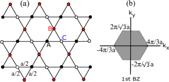
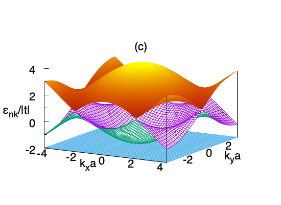
Figure 1: Sketches of (a) the crystal structure in real space and (b) the first Brillouin zone in reciprocal space. (c) Band structure with a flat band at the bottom. Note that while the flat band is in quadratic touch with a dispersive band at the origin, the dispersive bands touch each other and form Dirac cones at the six corners of the Brillouin zone.

The Hamiltonian for a single spin-$\sigma=\{\uparrow,\downarrow\}$ particle can be written as $\mathcal{H}_{\sigma}=\sum_{\mathbf{k}}\psi_{\mathbf{k}\sigma}^{\dagger}\mathbf{H}_{\mathbf{k}\sigma}\psi_{\mathbf{k}\sigma},$ where $\psi_{\mathbf{k}\sigma}=(c_{A\mathbf{k}\sigma}\;c_{B\mathbf{k}\sigma}\;c_{C\mathbf{k}\sigma})^{\mathrm{T}}$ is a three-component spinor with $\mathrm{T}$ the transpose operator and $c_{S\mathbf{k}\sigma}$ the annihilation operator for a spin-$\sigma$ particle on the sublattice $S$ with a crystal momentum $\mathbf{k}=(k_{x},k_{y})$. In the orbital basis $|S\mathbf{k}\sigma\rangle=c_{S\mathbf{k}\sigma}^{\dagger}|0\rangle$ with $|0\rangle$ the vacuum state, the Hamiltonian density can be written as

$$\mathbf{H}_{\mathbf{k}\sigma}=-2t\begin{bmatrix}0&\cos\left(\frac{\mathbf{k}\cdot\mathbf{a}_{2}}{2}\right)&\cos\left(\frac{\mathbf{k}\cdot\mathbf{a}_{1}}{2}\right)\\ \cos\left(\frac{\mathbf{k}\cdot\mathbf{a}_{2}}{2}\right)&0&\cos\left(\frac{\mathbf{k}\cdot\mathbf{a}_{3}}{2}\right)\\ \cos\left(\frac{\mathbf{k}\cdot\mathbf{a}_{1}}{2}\right)&\cos\left(\frac{\mathbf{k}\cdot\mathbf{a}_{3}}{2}\right)&0\end{bmatrix},$$ (1)

where $t$ is the hopping element between the nearest-neighbor lattice sites. The single-particle spectrum $\varepsilon_{n\mathbf{k}\sigma}$ is given by the eigenvalues of $\mathbf{H}_{\mathbf{k}\sigma}$, leading to barreteau17 ; mizoguchi19

$$\varepsilon_{1\mathbf{k}\sigma} =2t,$$ (2)

$$\varepsilon_{2\mathbf{k}\sigma} =-t-|t|\sqrt{2\Lambda_{\mathbf{k}}+3},$$ (3)

$$\varepsilon_{3\mathbf{k}\sigma} =-t+|t|\sqrt{2\Lambda_{\mathbf{k}}+3},$$ (4)

which are independent of the spin of the particle. Here the first band is flat and non-dispersive in $\mathbf{k}$ space, and the dispersive bands are characterized by $\Lambda_{\mathbf{k}}=\sum_{i=1}^{3}\cos(\mathbf{k}\cdot\mathbf{a}_{i}).$ We choose a negative $t=-|t|$ in this paper leading to a flat band at the bottom. The resultant band structure is shown in Fig. 1(c). We note that while the flat band is in quadratic touch with a dispersive band at $\mathbf{k=0}$, the dispersive bands touch each other and form Dirac cones at the six corners of the Brillouin zone.

Given our interest in the dispersion of the two-body bound states, we need not only the band structure but also the associated Bloch states $|n\mathbf{k}\sigma\rangle$. Thus a compact way to express the eigenvectors of $\mathbf{H}_{\mathbf{k}\sigma}$ is barreteau17 ; mizoguchi19

$$|1\mathbf{k}\sigma\rangle\equiv\begin{pmatrix}1_{A\mathbf{k}\sigma}\\ 1_{B\mathbf{k}\sigma}\\ 1_{C\mathbf{k}\sigma}\end{pmatrix} =\mathcal{A}_{1\mathbf{k}}\begin{bmatrix}\sin(\theta_{2\mathbf{k}}-\theta_{3\mathbf{k}})\\ \sin(\theta_{3\mathbf{k}}-\theta_{1\mathbf{k}})\\ \sin(\theta_{1\mathbf{k}}-\theta_{2\mathbf{k}})\end{bmatrix},$$ (5)

$$|2\mathbf{k}\sigma\rangle\equiv\begin{pmatrix}2_{A\mathbf{k}\sigma}\\ 2_{B\mathbf{k}\sigma}\\ 2_{C\mathbf{k}\sigma}\end{pmatrix} =\mathcal{A}_{2\mathbf{k}}\begin{bmatrix}\sin(\theta_{1\mathbf{k}}+\phi_{\mathbf{k}})\\ \sin(\theta_{2\mathbf{k}}+\phi_{\mathbf{k}})\\ \sin(\theta_{3\mathbf{k}}+\phi_{\mathbf{k}})\end{bmatrix},$$ (6)

$$|3\mathbf{k}\sigma\rangle\equiv\begin{pmatrix}3_{A\mathbf{k}\sigma}\\ 3_{B\mathbf{k}\sigma}\\ 3_{C\mathbf{k}\sigma}\end{pmatrix} =\mathcal{A}_{3\mathbf{k}}\begin{bmatrix}\cos(\theta_{1\mathbf{k}}+\phi_{\mathbf{k}})\\ \cos(\theta_{2\mathbf{k}}+\phi_{\mathbf{k}})\\ \cos(\theta_{3\mathbf{k}}+\phi_{\mathbf{k}})\end{bmatrix},$$ (7)

where $n_{S\mathbf{k}\sigma}=\langle S|n\mathbf{k}\sigma\rangle$ is the projection of the Bloch state onto the $S$th sublattice, $\mathcal{A}_{n\mathbf{k}}$ is the normalization factor, and $\theta_{1\mathbf{k}}=k_{x}a/4+k_{y}a/(4\sqrt{3}),$ $\theta_{2\mathbf{k}}=-k_{y}a/(2\sqrt{3}),$ $\theta_{3\mathbf{k}}=-k_{x}a/4+k_{y}a/(4\sqrt{3})$ and $\phi_{\mathbf{k}}=\frac{1}{2}\mathrm{arg}[e^{ik_{y}a/\sqrt{3}}+2\cos(k_{x}a/2)e^{-ik_{y}/(2\sqrt{3})}]$ are some phase factors associated with the geometry of the Kagome lattice. Having completed the analysis of the one-body problem, next we proceed with the two-body problem.

II.2 Two-body bound states

In the presence of a multiband tight-binding lattice, it is possible to solve the two-body problem exactly through a variational approach that is based on the following ansatz iskin21

$$|\Psi_{\mathbf{q}}\rangle=\sum_{nm\mathbf{k}}\alpha_{nm\mathbf{k}}^{\mathbf{q}}c_{n,\mathbf{k}+\mathbf{q}/2,\uparrow}^{\dagger}c_{m,-\mathbf{k}+\mathbf{q}/2,\downarrow}^{\dagger}|0\rangle.$$ (8)

Here $\mathbf{q}$ is the center-of-mass momentum of the spin-singlet bound pair that is formed between a spin-$\uparrow$ and a spin-$\downarrow$ particle, the variational parameter $\alpha_{nm\mathbf{k}}^{\mathbf{q}}$ is a complex number in general, and the operator $c_{n\mathbf{k}\sigma}^{\dagger}$ creates a particle in the Bloch state $|n\mathbf{k}\sigma\rangle=c_{n\mathbf{k}\sigma}^{\dagger}|0\rangle.$ The creation operators in the orbital and Bloch basis are related through $c_{n\mathbf{k}\sigma}^{\dagger}=\sum_{S}n_{S\mathbf{k}\sigma}c_{S\mathbf{k}\sigma}^{\dagger}$ since $\sum_{S}|S\mathbf{k}\sigma\rangle\langle S\mathbf{k}\sigma|=\mathcal{I}_{N_{b}}$ is an identity operator in $N_{b}$ dimensions for a given $\mathbf{k}$ and $\sigma$. The dispersion $E_{\ell\mathbf{q}}$ of the bound state is determined through the minimization of $\langle\Psi_{\mathbf{q}}|\mathcal{H}-E_{\ell\mathbf{q}}|\Psi_{\mathbf{q}}\rangle=0$ with respect to $\alpha_{nm\mathbf{k}}^{\mathbf{q}}$, where $\mathcal{H}=\mathcal{H}_{\uparrow}+\mathcal{H}_{\downarrow}+\mathcal{H}_{\uparrow\downarrow}$ is the total Hamiltonian of the system. Here we limit our analysis to an onsite (i.e., contact) attraction between the particles thanks mainly to the clarity of the central theme of this paper. For this purpose let us consider $\mathcal{H}_{\uparrow\downarrow}=-U\sum_{Si}\rho_{Si\uparrow}\rho_{Si\downarrow},$ where $U\geq 0$ is the strength of the interaction and $\rho_{Si\sigma}=c_{Si\sigma}^{\dagger}c_{Si\sigma}$ is the number operator at the $S$th sublattice in the $i$th unit cell. Here the operator $c_{Si\sigma}$ corresponds to the Fourier transform of $c_{S\mathbf{k}\sigma}$. In addition we take advantage of the time-reversal symmetry, and set $n_{S\mathbf{k}\uparrow}=n_{S,-\mathbf{k},\downarrow}^{*}\equiv n_{S\mathbf{k}}$ and $\varepsilon_{n\mathbf{k}\uparrow}=\varepsilon_{n,-\mathbf{k},\downarrow}\equiv\varepsilon_{n\mathbf{k}}.$ After some straightforward algebra iskin21 , $E_{\ell\mathbf{q}}$ is characterized by a set of linear equations

$$\mathbf{G^{q}}\boldsymbol{\beta}_{\ell\mathbf{q}}=0,$$ (9)

where $\mathbf{G^{q}}$ is an $N_{b}$-dimensional Hermitian matrix with the following elements

$$G_{SS^{\prime}}^{\mathbf{q}}=\delta_{SS^{\prime}}-\frac{U}{N_{c}}\sum_{nmS^{\prime}\mathbf{k}}\frac{m_{S\mathbf{K^{\prime}}}^{*}n_{S\mathbf{K}}n_{S^{\prime}\mathbf{K}}^{*}m_{S^{\prime}\mathbf{K^{\prime}}}}{\varepsilon_{n\mathbf{K}}+\varepsilon_{m\mathbf{K^{\prime}}}-E_{\ell\mathbf{q}}}.$$ (10)

Here $\mathbf{K}=\mathbf{k}+\mathbf{q}/2$ and $\mathbf{K^{\prime}}=\mathbf{k}-\mathbf{q}/2.$ Thus $E_{\ell\mathbf{q}}$ is determined by setting $\det\mathbf{G^{q}}=0$, and there are $N_{b}$ solutions for a given $\mathbf{q}$. We label these solutions with $\ell=\{1,2,3\}$ starting from the lower branch. Furthermore the state vector $\boldsymbol{\beta}_{\ell\mathbf{q}}=(\beta_{A\ell\mathbf{q}}\;\beta_{B\ell\mathbf{q}}\;\beta_{C\ell\mathbf{q}})^{\mathrm{T}}$ with $\beta_{S\ell\mathbf{q}}=\sum_{nm\mathbf{k}}\alpha_{nm\mathbf{k}}^{\mathbf{q}}n_{S\mathbf{K}}m_{S\mathbf{K^{\prime}}}^{*}$ is the corresponding eigenvector of $\mathbf{G^{q}}$, and it carries further insight into the physical mechanism and nature of the bound state.

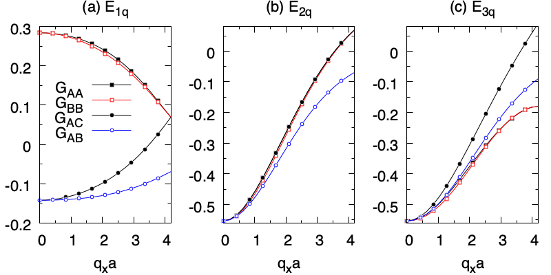
Figure 2: Matrix elements $G_{SS^{\prime}}^{\mathbf{q}}$ for $U=2|t|$ as a function of $q_{x}$ when $q_{y}=0$. Here (a), (b) and (c) corresponds, respectively, to the self-consistent solutions for $E_{1\mathbf{q}}$, $E_{2\mathbf{q}}$ and $E_{3\mathbf{q}}$. Since $G_{CC}^{\mathbf{q}}=G_{AA}^{\mathbf{q}}$ and $G_{BC}^{\mathbf{q}}=G_{AB}^{\mathbf{q}}$ for all $q_{x}$, these coefficients are not shown. Note that $G_{AA}^{\mathbf{q}}=G_{BB}^{\mathbf{q}}$ and $G_{AB}^{\mathbf{q}}=G_{AC}^{\mathbf{q}}$ in the small-$q_{x}a$ limit. In addition, together with the characteristic (bound-state) Eq. (9), these coefficients imply $\beta_{1\mathbf{q}}\propto(1,1,1)$, $\beta_{2\mathbf{q}}\propto(1,0,-1)$ and $\beta_{3\mathbf{q}}\propto(1,-2,1)$ in the small-$q_{x}a$ limit.

Our numerical calculations for the Kagome lattice show that the matrix elements of $\mathbf{G^{q}}$ have the following properties. When $\mathbf{q}$ is along one of the principal axis, i.e., either when $q_{x}=0$ or $q_{y}=0$, we observed that $G_{AA}^{\mathbf{q}}=G_{CC}^{\mathbf{q}}$ and $G_{AB}^{\mathbf{q}}=G_{BC}^{\mathbf{q}}$ for all parameters. Thus one of the eigenvalues of $\mathbf{G^{q}}=0$ is $G_{AA}^{\mathbf{q}}-G_{AC}^{\mathbf{q}}$ with the eigenvector $\beta_{2\mathbf{q}}\propto(1,0,-1),$ and it determins the middle branch $E_{2\mathbf{q}}$. The upper branch $E_{3\mathbf{q}}$ and the lower one $E_{1\mathbf{q}}$ are determined, respectively, by the eigenvalues $(G_{AA}^{\mathbf{q}}+G_{BB}^{\mathbf{q}}+G_{AC}^{\mathbf{q}})/2\pm[8(G_{AA}^{\mathbf{q}})^{2}+(G_{AC}^{\mathbf{q}})^{2}+(G_{AA}^{\mathbf{q}}-G_{BB}^{\mathbf{q}})(2G_{AC}^{\mathbf{q}}+G_{AA}^{\mathbf{q}}-G_{BB}^{\mathbf{q}})]^{1/2}/2,$ where $\beta_{3\mathbf{q}}\propto(1,Q_{\mathbf{q}},1)$ with $Q_{\mathbf{q}}<0$ and $\beta_{1\mathbf{q}}\propto(1,R_{\mathbf{q}},1)$ with $R_{\mathbf{q}}>0$. While the $\mathbf{q}$ dependences of $Q_{\mathbf{q}}$ and $R_{\mathbf{q}}$ are not very illuminating and skipped, they are in such a way that $Q_{\mathbf{q}}R_{\mathbf{q}}=-2$ for every $\mathbf{q}$ which is required by the orthonormalization of $\boldsymbol{\beta}_{\ell\mathbf{q}}$. Thus, by setting the eigenvalues of $\mathbf{G^{q}}$ to 0, we find that $E_{2\mathbf{q}}$ is determined by the condition $G_{AA}^{\mathbf{q}}=G_{AC}^{\mathbf{q}},$ and that $E_{1\mathbf{q}}$ and $E_{3\mathbf{q}}$ are determined by the same condition $2(G_{AB}^{\mathbf{q}})^{2}=G_{BB}^{\mathbf{q}}(G_{AA}^{\mathbf{q}}+G_{AC}^{\mathbf{q}}).$ On the other hand, when $q=\sqrt{q_{x}^{2}+q_{y}^{2}}$ is small, i.e., when $qa\ll 1$, we observed that $G_{AA}^{\mathbf{q}}=G_{BB}^{\mathbf{q}}=G_{CC}^{\mathbf{q}}$ and $G_{AB}^{\mathbf{q}}=G_{BC}^{\mathbf{q}}=G_{AC}^{\mathbf{q}}$ for all parameters. These are shown in Fig. 2. Thus $E_{1\mathbf{q}}$ is determined by the condition $G_{AA}^{\mathbf{q}}=-2G_{AB}^{\mathbf{q}},$ and it is characterized by $\beta_{1\mathbf{q}}\propto(1,1,1)$. This suggests that the low-energy bound states can be distinguished by their perfectly in-phase (i.e., spatially-uniform) contribution from all three sublattices twobandnote . On the other hand $E_{2\mathbf{q}}$ and $E_{3\mathbf{q}}$ are both determined by the very same condition $G_{AA}^{\mathbf{q}}=G_{AB}^{\mathbf{q}}$ (i.e., they are degenerate in the small-$q$ limit), and are characterized, respectively, by $\beta_{2\mathbf{q}}\propto(1,0,-1)$ and $\beta_{3\mathbf{q}}\propto(1,-2,1)$.

As an illustration we set $U=2|t|$ and $q_{y}=0$ in Fig. 3(a), and present the two-body spectrum $E_{\ell\mathbf{q}}$ as a function of $q_{x}$. Even though $E_{3\mathbf{q}}$ disperses in $\mathbf{q}$, it appears quite flat and featureless in the presented scale. We observe that while $E_{3\mathbf{q}}$ and $E_{2\mathbf{q}}$ are degenerate at low $q$, $E_{2\mathbf{q}}$ and $E_{1\mathbf{q}}$ are degenerate at the corner of the Brillouin zone. More importantly the quadratic expansion of $E_{1\mathbf{q}}=E_{b}+q^{2}/(2M_{b})$ provides an excellent fit for the lower branch in the small-$q$ limit, where $E_{b}\approx-4.934|t|$ is the energy of the lowest bound state and $M_{b}\approx 12.574/(|t|a^{2})$ is its effective mass. We remark here that the effective masses of $E_{1\mathbf{q}}$ and $E_{2\mathbf{q}}$ branches become very close to each other (in magnitude) as $U$ gets larger and larger. In order to gain deeper insight into the former result, next we use our observation that $\beta_{1\mathbf{q}}\propto(1,1,1)$ for the lower band in the small-$q$ limit. Furthermore this observation allows us to derive the generalized relation between the inverse of the effective-mass tensor of the lowest bound states and the quantum-metric tensor of the underlying Bloch states for those multiband lattices that simultaneously exhibit time-reversal symmetry and fulfill the condition on spatially-uniform pairing.

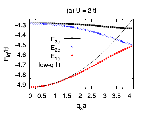
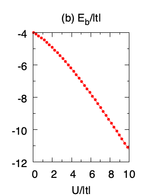
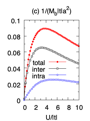
Figure 3: (a) Two-body spectrum $E_{\ell\mathbf{q}}$ for $U=2|t|$ as a function of $q_{x}$ when $q_{y}=0$. The quadratic expansion of $E_{1\mathbf{q}}=E_{b}+q^{2}/(2M_{b})$ is an excellent fit for the lower branch in the small-$q$ limit. (b) $E_{b}$ as a function of $U$. (c) $1/M_{b}=1/M_{b}^{\mathrm{intra}}+1/M_{b}^{\mathrm{inter}}$ as a function of $U$ along with its intraband and interband contributions, where $1/M_{b}^{\mathrm{inter}}=1/M_{b}^{\mathrm{inter,1}}+1/M_{b}^{\mathrm{inter,2}}.$

III Relation to quantum metric

Given our numerical observation that the small-$q$ limit of the lower branch $E_{1\mathbf{q}}$ is characterized by $\beta_{1\mathbf{q}}\propto(1,1,1),$ it is possible to isolate the condition that determines $E_{1\mathbf{q}}$ as $\sum_{SS^{\prime}}G_{SS^{\prime}}^{\mathbf{q}}=0.$ This is a very convenient form, and it may find practical applications in other multiband lattices as long as the lowest bound states are distinguished by a perfectly in-phase contribution from all of the sublattices, i.e., $\beta_{1\mathbf{q}}\propto(1,1,\dots,1).$ Hoping that this is generically the case in time-reversal-symmetric systems with a spatially-uniform pairing, below we keep the formalism and the discussion general. By plugging Eq. (10) into this condition, and observing that $\sum_{S}m_{S\mathbf{K^{\prime}}}^{*}n_{S\mathbf{K}}=\langle m_{\mathbf{K^{\prime}}}|n_{\mathbf{K}}\rangle$ with $|n_{\mathbf{K}}\rangle$ representing the Bloch states that are given in Eqs. (5-7), we obtain a much simpler condition

$$1=\frac{U}{N}\sum_{nm\mathbf{k}}\frac{|\langle m_{\mathbf{k}-\mathbf{q}/2}|n_{\mathbf{k}+\mathbf{q}/2}\rangle|^{2}}{\varepsilon_{n,\mathbf{k}+\mathbf{q}/2}+\varepsilon_{m,\mathbf{k}-\mathbf{q}/2}-E_{1\mathbf{q}}}.$$ (11)

Here $N=N_{b}N_{c}$ is the total number of lattice sites in the system. This expression can be used to make further analytical progress by taking its small-$q$ limit.

For instance, in the presence of an energetically-isolated flat band $\varepsilon_{f\mathbf{k}}=\varepsilon_{f}$ that is separated from the remaining bands with a finite band gap, Eq. (11) can be approximated by $1=(U/N)\sum_{\mathbf{k}}|\langle f_{\mathbf{k}-\mathbf{q}/2}|f_{\mathbf{k}+\mathbf{q}/2}\rangle|^{2}/(2\varepsilon_{f}-E_{1\mathbf{q}})$ in the small-$U$ limit, leading to torma18 $E_{1\mathbf{q}}=2\varepsilon_{f}-(U/N)\sum_{\mathbf{k}}|\langle f_{\mathbf{k}-\mathbf{q}/2}|f_{\mathbf{k}+\mathbf{q}/2}\rangle|^{2}.$ Furthermore we use the Taylor expansions $|f_{\mathbf{k}\pm\mathbf{q}/2}\rangle=|f_{\mathbf{k}}\pm(1/2)\sum_{i}q_{i}\partial_{i}f_{\mathbf{k}}+(1/8)\sum_{ij}q_{i}q_{j}\partial_{i}\partial_{j}f_{\mathbf{k}}\rangle$ in small $\mathbf{q}$ and obtain $|\langle f_{\mathbf{k}-\mathbf{q}/2}|f_{\mathbf{k}+\mathbf{q}/2}\rangle|^{2}=1-(1/2)\sum_{ij}q_{i}q_{j}g_{ij}^{f\mathbf{k}}.$ This is exact up to second order in $\mathbf{q}$ where $g_{ij}^{n\mathbf{k}}=\mathrm{Tr}\big{(}\partial_{i}P_{n_{\mathbf{k}}}\partial_{j}P_{n_{\mathbf{k}}}\big{)}$ is the matrix element of the so-called quantum-metric tensor of the Bloch state $|n_{\mathbf{k}}\rangle$ resta11 . Here $\mathrm{Tr}$ is the trace, $\partial_{i}=\partial/\partial k_{i}$ is the partial derivative, and $P_{n_{\mathbf{k}}}=|n_{\mathbf{k}}\rangle\langle n_{\mathbf{k}}|$ is the projection operator. Since $P_{n_{\mathbf{k}}}$ is a gauge-independent operator by definition, $g_{ij}^{n\mathbf{k}}$ is also a band invariant. By noting that $\langle n_{\mathbf{k}}|\partial_{i}n_{\mathbf{k}}\rangle=-\langle\partial_{i}n_{\mathbf{k}}|n_{\mathbf{k}}\rangle$ is an imaginary number due to the normalization $\langle n_{\mathbf{k}}|n_{\mathbf{k}}\rangle=1$ of the Bloch states, the quantum metric can be reexpressed in a more familiar form provost80 ; berry89 ; resta11

$$g_{ij}^{n\mathbf{k}}=2\mathrm{Re}\langle\partial_{i}n_{\mathbf{k}}|(\mathcal{I}_{N_{b}}-|n_{\mathbf{k}}\rangle\langle n_{\mathbf{k}}|)|\partial_{j}n_{\mathbf{k}}\rangle,$$ (12)

where $\mathrm{Re}$ is the real part of the expression. As a result we eventually find (i.e., to the lowest order in $\mathbf{q}$)

$$E_{1\mathbf{q}}=E_{b}+\frac{1}{2}\sum_{ij}q_{i}q_{j}(M_{b}^{-1})_{ij},$$ (13)

where $E_{b}=2\varepsilon_{f}-U/N_{b}$ is the threshold energy and $(M_{b}^{-1})_{ij}=(U/N)\sum_{\mathbf{k}}g_{ij}^{f\mathbf{k}}$ is the matrix element of the inverse of the effective-mass tensor $\mathbf{M_{b}}$. We remark here that these expressions are strictly valid in the small-$U$ limit assuming an energetically-isolated flat band torma18 .

Similarly one can perform a small-$\mathbf{q}$ expansion of Eq. (11) and generalize $E_{b}$ and $\mathbf{M}_{\mathbf{b}}^{-1}$ not only to arbitrary $U$ values but also to arbitrary band structures. For this purpose we first use the Taylor expansions of $|n_{\mathbf{k}\pm\mathbf{q}/2}\rangle$ given above and find $\langle m_{\mathbf{k}-\mathbf{q}/2}|n_{\mathbf{k}+\mathbf{q}/2}\rangle=\delta_{mn}+\sum_{i}q_{i}\langle m_{\mathbf{k}}|\partial_{i}n_{\mathbf{k}}\rangle-(1/8)\sum_{ij}q_{i}q_{j}(3\langle\partial_{i}m_{\mathbf{k}}|\partial_{j}n_{\mathbf{k}}\rangle+\langle\partial_{j}m_{\mathbf{k}}|\partial_{i}n_{\mathbf{k}}\rangle),$ where $\langle m_{\mathbf{k}}|n_{\mathbf{k}}\rangle=\delta_{mn}$ is due to the orthonormalization of the Bloch states and $\langle m_{\mathbf{k}}|\partial_{i}n_{\mathbf{k}}\rangle=-\langle\partial_{i}m_{\mathbf{k}}|n_{\mathbf{k}}\rangle.$ This leads to $|\langle m_{\mathbf{k}-\mathbf{q}/2}|n_{\mathbf{k}+\mathbf{q}/2}\rangle|^{2}=\delta_{mn}-\mathrm{Re}\sum_{ij}q_{i}q_{j}\langle\partial_{i}n_{\mathbf{k}}|(\delta_{mn}-|m_{\mathbf{k}}\rangle\langle m_{\mathbf{k}}|)|\partial_{j}n_{\mathbf{k}}\rangle$ in the small-$\mathbf{q}$ limit. Then we expand the single-particle spectrum $\varepsilon_{n,\mathbf{k}\pm\mathbf{q}/2}=\varepsilon_{n\mathbf{k}}\pm(1/2)\sum_{i}q_{i}\partial_{i}\varepsilon_{n\mathbf{k}}+(1/8)\sum_{ij}q_{i}q_{j}\partial_{i}\partial_{j}\varepsilon_{n\mathbf{k}}$ up to second order in $\mathbf{q}$ and plug Eq. (13) for the dispersion of the lowest bound states. By matching the coefficient of the zeroth order terms in Eq. (11), we find

$$1=\frac{U}{N}\sum_{n\mathbf{k}}\frac{1}{2\varepsilon_{n\mathbf{k}}-E_{b}},$$ (14)

which is the self-consistency relation for the energy $E_{b}$ of the lowest bound state. The first-order terms already vanish. By requiring that the second-order terms vanish, we find a closed-form expression for $\mathbf{M}_{\mathbf{b}}^{-1}=\mathbf{M}_{\mathrm{intra}}^{-1}+\mathbf{M}_{\mathrm{inter}}^{-1},$ where $\mathbf{M}_{\mathrm{intra}}^{-1}$ is the so-called conventional or the intraband and $\mathbf{M}_{\mathrm{inter}}^{-1}=\mathbf{M}_{\mathrm{inter,1}}^{-1}+\mathbf{M}_{\mathrm{inter,2}}^{-1}$ is the so-called geometric or the interband contribution to the inverse of the effective-mass tensor. They can be written as

$$(M_{\mathrm{intra}}^{-1})_{ij} =\frac{1}{2D}\sum_{n\mathbf{k}}\frac{\partial_{i}\partial_{j}\varepsilon_{n\mathbf{k}}}{(2\varepsilon_{n\mathbf{k}}-E_{b})^{2}},$$ (15)

$$(M_{\mathrm{inter,1}}^{-1})_{ij} =\frac{1}{D}\sum_{n\mathbf{k}}\frac{g_{ij}^{n\mathbf{k}}}{2\varepsilon_{n\mathbf{k}}-E_{b}},$$ (16)

$$(M_{\mathrm{inter,2}}^{-1})_{ij} =-\frac{1}{D}\sum_{n,m\neq n,\mathbf{k}}\frac{g_{ij}^{nm\mathbf{k}}}{\varepsilon_{n\mathbf{k}}+\varepsilon_{m\mathbf{k}}-E_{b}},$$ (17)

where $D=\sum_{n\mathbf{k}}\frac{1}{(2\varepsilon_{n\mathbf{k}}-E_{b})^{2}}$ and $E_{b}$ is determined by Eq. (14) for a given $U$. Here Eq. (17) depends on the so-called band-resolved quantum metric

$$g_{ij}^{nm\mathbf{k}}=2\mathrm{Re}\langle\partial_{i}n_{\mathbf{k}}|m_{\mathbf{k}}\rangle\langle m_{\mathbf{k}}|\partial_{j}n_{\mathbf{k}}\rangle,$$ (18)

since it produces the quantum metric of the $n$th band when summed over the rest of the bands, i.e., $g_{ij}^{n\mathbf{k}}=\sum_{m\neq n}g_{ij}^{nm\mathbf{k}}.$ Equations (15 - 17) constitute the generalized relation between the inverse of the effective-mass tensor of the lowest bound states and the quantum-metric tensor of the underlying Bloch states, and they are exact.

Let us now reproduce the known results using Eqs. (14 - 17). In the case of an energetically-isolated flat band $\varepsilon_{f\mathbf{k}}=\varepsilon_{f}$ that is separated from the remaining bands with a finite band gap, Eqs. (15) and (17) are negligible in the small-$U$ limit. Furthermore Eq. (16) is approximated by $(M_{\mathrm{inter,1}}^{-1})_{ij}=(U/N)\sum_{\mathbf{k}}g_{ij}^{f\mathbf{k}}$ in the small-$U$ limit where $2\varepsilon_{f}-E_{b}=U/N_{b}.$ These are in full agreement with the literature torma18 and the discussion given below Eq. (11). On the other hand, in the case of a two-band ($N_{b}=2$) lattice that is described by the Hamiltonian density $H_{\mathbf{k}\sigma}=d_{0}^{\mathbf{k}}\mathcal{I}_{2}+\mathbf{d}_{\mathbf{k}}\cdot\boldsymbol{\tau},$ the single-particle spectrum is given by $\varepsilon_{s\mathbf{k}}=d_{0}^{\mathbf{k}}+sd_{\mathbf{k}}$ where $s=\{+,-\}$ labels, respectively, the upper and lower bands. Here $\boldsymbol{\tau}=(\tau_{x},\tau_{y},\tau_{z})$ is a vector of Pauli matrices in the two-dimensional orbital basis. In this case the quantum metrics of the two bands are equal to each other, i.e., $g_{ij}^{+,\mathbf{k}}=g_{ij}^{-,\mathbf{k}},$ given that $g_{ij}^{s\mathbf{k}}=2\mathrm{Re}\langle\partial_{i}s_{\mathbf{k}}|(-s)_{\mathbf{k}}\rangle\langle(-s)_{\mathbf{k}}|\partial_{j}s_{\mathbf{k}}\rangle$ and $\sum_{s\mathbf{k}}|s_{\mathbf{k}}\rangle\langle s_{\mathbf{k}}|=\mathcal{I}_{2}.$ For this reason Eq. (17) can be written as $\sum_{s\mathbf{k}}g_{ij}^{s\mathbf{k}}/(2d_{0}^{\mathbf{k}}-E_{b}),$ leading to $(M_{\mathrm{inter}}^{-1})_{ij}=-\frac{2}{D}\sum_{s\mathbf{k}}\frac{sd_{\mathbf{k}}g_{ij}^{s\mathbf{k}}}{(2\varepsilon_{s\mathbf{k}}-E_{b})(2d_{0}^{\mathbf{k}}-E_{b})}.$ These are again in full agreement with the literature iskin21 .

Lastly we apply Eqs. (14 - 17) to the Kagome lattice and solve them self-consistently for $E_{b}$ and $M_{b}$. Their numerical values are presented, respectively, in Figs. 3(b) and 3(c) as a function of $U$. In this particular case $\mathbf{M_{b}}$ is an isotropic matrix with $(M_{b}^{-1})_{ij}=\delta_{ij}/M_{b}.$ We find that while $E_{b}=-4|t|-U/3$ increases linearly in the small-$U$ limit due to the presence of a flat lower band in a three-band lattice, $E_{b}=-U$ in the large-$U$ limit which is similar to what happens in a one-band lattice. Similarly while $M_{b}=r_{1}/[a^{2}U\ln(r_{2}|t|/U)]$ diverges logarithmically in the small-$U$ limit due to the presence of a band touching with a non-isolated flat band, $M_{b}=U/(a^{2}t^{2})$ increases linearly in the large-$U$ limit which is again similar to what happens in a one-band lattice. Here $r_{1}$ and $r_{2}$ are real positive constants. In comparison, in the absence of a band touching (i.e., for an isolated flat band), we note that $M_{b}=r_{3}/(a^{2}U)$ diverges with a power law in the small-$U$ limit torma18 . Furthermore we find that $E_{b}\approx-4.934|t|$ and $M_{b}\approx 12.574/(|t|a^{2})$ when $U=2|t|$, and they provide a perfect fit for the exact results in the small-$q$ limit. This is shown in Fig. 3(a).

We note in passing that $1/M_{b}^{\mathrm{inter,1}}>0$ is in direct competition with $1/M_{b}^{\mathrm{inter,2}}<0$, and their magnitudes are about three orders of magnitude larger than $1/M_{b}^{\mathrm{intra}}$. However their sum $1/M_{b}^{\mathrm{inter}}=1/M_{b}^{\mathrm{inter,1}}+1/M_{b}^{\mathrm{inter,2}}$ is quite comparable to $1/M_{b}^{\mathrm{intra}}$ as can be seen in Fig. 3(c). Having shown that Eqs. (15-17) are exact for the Kagome lattice for all $U$ values, next we discuss their versatility for other lattices.

IV Spatially-Uniform Pairing

In accordance with the analysis presented above, Eqs. (15-17) are clearly exact for those multiband lattices that simultaneously fulfill the following conditions: (i) the Bloch Hamiltonian must exhibit time-reversal symmetry and (ii) the resultant two-body wave function must have a uniform contribution from all of the underlying sublattices. The latter is the so-called spatially-uniform-pairing condition, and it is expected to be satisfied by those Bloch Hamiltonians that are invariant under the interchange of their sublattices. Note that if the condition (ii) is satisfied for the two-body problem in a lattice then we expect the mean-field pairing order parameter ($\Delta_{Si}=\Delta_{S}$) for the many-body problem to be spatially-uniform, i.e., $\Delta_{S}=\Delta$ is equal for all of the sublattices.

In the case of two-band lattices while the honeycomb, Mielke checkerboard, Kane-Mele, Creutz and Haldane type Hubbard models with onsite interactions are among those popular lattices that satisfy condition (ii), i.e., because of their inversion symmetry, the sawtooth and zigzag type models are not. Here we note that the time-reversal symmetry is broken for the Creutz and Haldane models. In the case of three-band lattices, while the Kagome lattice with onsite interaction satisfy condition (ii), the Lieb and dice lattices do not since only two of their sublattices are interchangeable with each other but not the third one. According to the recent findings torma18 ; wu21 , the contribution to the two-body wave function from the non-interchangeable sublattice vanishes for both of these models in the small-$U$ limit. Because of this Eqs. (15-17) still work for these models but only in the $U/t\to 0$ limit. In particular, since the flat band of the Lieb lattice is isolated from the other bands with a gap, it is sufficient to keep only the flat-band contribution coming from Eq. (16) in the small-$U$ limit. However, since the flat band of the dice lattice is in touch with one of the dispersive bands, one needs to keep both the flat-band contribution and that of the touching band coming from Eqs. (15-17) in the small-$U$ limit.

V Conclusion

To summarize here we considered an onsite attraction $U$ between a spin-$\uparrow$ and a spin-$\downarrow$ fermion in a multiband lattice, and derived an exact relation between the inverse of the effective-mass tensor $(M_{b}^{-1})_{ij}$ of the lowest bound states $E_{1\mathbf{q}}$ and the quantum-metric tensor $g_{ij}^{n\mathbf{k}}$ of the underlying Bloch states $|n_{\mathbf{k}}\rangle$. In addition to the intraband contribution $(M_{\mathrm{intra}}^{-1})_{ij}$ that depends only on the single-particle spectrum $\varepsilon_{n\mathbf{k}}$ and the interband contribution $(M_{\mathrm{inter,1}}^{-1})_{ij}$ that is controlled by $g_{ij}^{n\mathbf{k}}$, our generalized relation has an additional interband contribution $(M_{\mathrm{inter,2}}^{-1})_{ij}$ that depends on the band-resolved quantum metric $g_{ij}^{nm\mathbf{k}}$. Our analytical expression is applicable to those multiband lattices that simultaneously exhibit time-reversal symmetry and fulfill the condition on spatially-uniform pairing. It reproduces the previously known results including that of isolated flat bands in the small-$U$ limit torma18 and that of two-band lattices for arbitrary $U$ iskin21 . Furthermore we also solved the two-body problem in a Kagome lattice with nearest-neighbor hoppings, and showed that the exact relation provides a perfect benchmark for this three-band lattice. In general it is probably not possible to isolate the geometric contributions to the effective mass, and study their effects alone in the experiments. However our results for a flat band show that the geometric contributions play a dominant role in the small-$U$ limit, and can be studied there. As an outlook our exact relation may find direct applications in many other lattices including those of the Moire materials topp21 , motivated by the hope that the formation of a two-body bound state can be used as a precursor to superconductivity in these systems.

- (1) J. P. Provost and G. Vallee, Riemannian structure on manifolds of quantum states, Commun. Math. Phys. 76, 289 (1980).
- (2) M. V. Berry, The quantum phase, five years after in Geometric Phases in Physics, edited by A. Shapere and F. Wilczek (World Scientific, Singapore, 1989).
- (3) R. Resta, The insulating state of matter: A geometrical theory, Eur. Phys. J. B 79, 121 (2011).
- (4) S. Peotta and P. Törmä, Superfluidity in topologically nontrivial flat bands, Nat. Commun. 6, 8944 (2015).
- (5) A. Julku, S. Peotta, T. I. Vanhala, D.-H. Kim, and P. Törmä, Geometric Origin of Superfluidity in the Lieb-Lattice Flat Band, Phys. Rev. Lett. 117, 045303 (2016).
- (6) L. Liang, T. I. Vanhala, S. Peotta, T. Siro, A. Harju, and P. Törmä, Band geometry, Berry curvature, and superfluid weight, Phys. Rev. B 95, 024515 (2017).
- (7) M. Iskin, Quantum metric contribution to the pair mass in spin-orbit coupled Fermi superfluids, Phys. Rev. A 97, 033625 (2018).
- (8) M. Iskin, Origin of flat-band superfluidity on the Mielke checkerboard lattice, Phys. Rev. A 99, 053608 (2019).
- (9) Z. Wang, G. Chaudhary, Q. Chen, and K. Levin, Quantum geometric contributions to the BKT transition: Beyond mean field theory, Phys. Rev. B 102, 184504 (2020).
- (10) M. Iskin, Collective excitations of a BCS superfluid in the presence of two sublattices, Phys. Rev. A 101, 053631 (2020).
- (11) Y.-R. Wu, X.-F. Zhang, C.-F. Liu, W.-M. Liu, and Y.-C. Zhang, Superfluid density and collective modes of fermion superfluid in dice lattice, Sci. Rep. 11, 13572 (2021).
- (12) L. Asteria, D. T. Tran, T. Ozawa, M. Tarnowski, B. S. Rem, N. Fl schner, K. Sengstock, N. Goldman, and C. Weitenberg, Measuring quantized circular dichroism in ultracold topological matter, Nat. Phys. 15, 449 (2019).
- (13) M. Yu, P. Yang, M. Gong, Q. Cao, Q. Lu, H. Liu, S. Zhang, M. B. Plenio, F. Jelezko, T. Ozawa, N. Goldman, S. Zhang, and J. Cai, Experimental measurement of the quantum geometric tensor using coupled qubits in diamond, Natl. Sci. Rev. 7, 254 (2020).
- (14) A. Gianfrate, O. Bleu, L. Dominici, V. Ardizzone, M. De Giorgi, D. Ballarini, G. Lerario, K. West, L. Pfeiffer, D. Solnyshkov, D. Sanvitto, and G. Malpuech, Measurement of the quantum geometric tensor and of the anomalous Hall drift, Nature 578, 381 (2020).
- (15) X. Tan, D.-W. Zhang, Z. Yang, J. Chu, Y.-Q. Zhu, D. Li, X. Yang, S. Song, Z. Han, Z. Li, Y. Dong, H.-F. Yu, H. Yan, S.-L. Zhu, and Y. Yu, Experimental measurement of the quantum metric tensor and related topological phase transition with a superconducting qubit, Phys. Rev. Lett. 122, 210401 (2019).
- (16) Q. Liao, C. Leblanc, J. Ren, F. Li, Y. Li, D. Solnyshkov, G. Malpuech, J. Yao, and H. Fu, Experimental Measurement of the Divergent Quantum Metric of an Exceptional Point, Phys. Rev. Lett. 127, 107402 (2021).
- (17) P. Törmä, L. Liang, and S. Peotta, Quantum metric and effective mass of a two-body bound state in a flat band, Phys. Rev. B 98, 220511(R) (2018).
- (18) M. Iskin, Two-body problem in a multiband lattice and the role of quantum geometry, Phys. Rev. A 103, 053311 (2021).
- (19) G.-B. Jo, J. Guzman, C. K. Thomas, P. Hosur, A. Vishwanath, and D. M. Stamper-Kurn, Ultracold Atoms in a Tunable Optical Kagome Lattice, Phys. Rev. Lett. 108, 045305 (2012).
- (20) Y. Nakata, T. Okada, T. Nakanishi, and M. Kitano, Observation of flat band for terahertz spoof plasmons in a metallic Kagomé lattice, Phys. Rev. B 85, 205128 (2012).
- (21) Z. Li, J. Zhuang, L. Wang, H. Feng, Q. Gao, X. Xu, W. Hao, X. Wang, C. Zhang, K. Wu, S. X. Dou, L. Chen, Z. Hu, and Y. Du, Realization of flat band with possible nontrivial topology in electronic Kagome lattice, Science Advances 4, eaau4511 (2018).
- (22) T.-H. Leung, M. N. Schwarz, S.-W. Chang, C. D. Brown, G. Unnikrishnan, and D. Stamper-Kurn, Interaction-Enhanced Group Velocity of Bosons in the Flat Band of an Optical Kagome Lattice, Phys. Rev. Lett. 125, 133001 (2020).
- (23) F. Diebel, D. Leykam, S. Kroesen, C. Denz, and A. S. Desyatnikov, Conical Diffraction and Composite Lieb Bosons in Photonic Lattices, Phys. Rev. Lett. 116, 183902 (2016).
- (24) S. Kajiwara, Y. Urade, Y. Nakata, T. Nakanishi, and M. Kitano, Observation of a nonradiative flat band for spoof surface plasmons in a metallic Lieb lattice, Phys. Rev. B 93, 075126 (2016).
- (25) H. Ozawa, S. Taie, T. Ichinose, and Y. Takahashi, Interaction-Driven Shift and Distortion of a Flat Band in an Optical Lieb Lattice, Phys. Rev. Lett. 118, 175301 (2017).
- (26) C. Barreteau, F. Ducastelle, and T. Mallah, A bird’s eye view on the flat and conic band world of the honeycomb and Kagome lattices: towards an understanding of 2D metal-organic frameworks electronic structure, J. Phys.: Condens. Matter 29, 465302 (2017).
- (27) T. Mizoguchi and M. Udagawa, Flat-band engineering in tight-binding models: Beyond the nearest-neighbor hopping, Phys. Rev. B 99, 235118 (2019).
- (28) In the case of two-band lattices there are two distinct branches in the two-body spectrum. Assuming onsite attraction and uniform pairing, it can be shown that the lower (upper) branch is associated with the Goldstone (Leggett) modes that describe the perfectly in-phase (out-of-phase) collective fluctuations of the superfluid order parameter on two different sublattices iskin21 . For this reason is a manifestation of the perfectly in-phase sublattice contribution to the pair formation.
- (29) G. E. Topp, C. J. Eckhardt, D. M. Kennes, M. A. Sentef, and P. Törmä, Light-matter coupling and quantum geometry in moiré materials, Phys. Rev. B 104, 064306 (2021).