The Stellar "Snake" I: Whole Structure and Properties

Abstract

To complement our previous discovery of the young snake-like structure in the solar neighborhood and reveal the structure’s full extent, we build two samples of stars within the Snake and its surrounding territory from Gaia EDR3. With the friends-of-friends algorithm, we identify 2694 and 9615 Snake member candidates from the two samples. Thirteen open clusters are embedded in these member candidates. By combining the spectroscopic data from multiple surveys, we investigate the comprehensive properties of the candidates and find that they are very likely to belong to one sizable structure, since most of the components are well bridged in their spatial distributions, and follow a single stellar population with an age of $30-40$ Myr and solar metallicity. This sizable structure is best explained as hierarchically primordial, and probably formed from a filamentary giant molecular cloud with unique formation history in localized regions. To analyze the dynamics of the Snake, we divide the structure into five groups according to their tangential velocities; we find that the groups are expanding at a coherent rate ($\kappa_{X}\sim 3.0\,\times 10^{-2}\,\rm km\,s^{-1}\,pc^{-1}$) along the length of the structure ($X$-direction). The corresponding expansion age ($\tau\sim 33$ Myr) is highly consistent with the age of the Snake. With over ten thousand member stars, the Snake is an ideal laboratory to study nearby coeval stellar formation, stellar physics, and environmental evolution over a large spatial extent.

1 Introduction

Filamentary structures have a long history of detection within Galactic giant molecular clouds (GMCs) (Schneider & Elmegreen, 1979; Su et al., 2015; Zucker et al., 2018; Soler et al., 2021); clouds of such type are the stellar factories of galaxies (Dobbs, 2013). One scenario of the evolution of these filaments results in elongated stellar structures, e.g., the stellar "Snake" – a young (only $30-40$ Myr) snake-like structure in the solar neighborhood (around 300 pc from the Sun) that was first reported by Tian (2020, hereafter T20). Besides bright O and B members, this structure includes a number of intermediate-mass stars and low-mass pre-main sequence (PMS) stars extending hundreds of parsecs. The Snake members are consistent with a single stellar population in the color-absolute magnitude diagram (CMD) and a continuous mass function. Thus the Snake is an ideal laboratory to study nearby coeval stellar formation, stellar physics, and environmental evolution over a large spatially extended region.

The Snake communes alongside several stellar populations of widely different ages as well as spatial and kinematic extent, for instance, the Vela-Puppis complex (Cantat-Gaudin et al., 2018, 2019a, 2019b, hereafter, CG18, CG19a, CG19b) and Orion complex (Kounkel et al., 2018a, hereafter, K18). The community includes tens of open clusters, associations, and groups; and many of these populations have been presented in the literature (e.g., K18; CG18; CG19a,b; de Zeeuw et al., 1999; Beccari et al., 2018; Armstrong et al., 2018; Zari et al., 2019; Armstrong et al., 2020; Pang et al., 2021). These populations are spatially not far from each other, and their average distance is around 300 pc from the Sun (CG18; Franciosini et al., 2018; Chen et al., 2020). In terms of age, they are young with ages $<$ 50 Myr (CG19b; Zari et al., 2019).

The age of the Vela-Puppis complex has been derived by several works in the literature (Dias et al., 2002; Kharchenko et al., 2013; Bossini et al., 2019). The average age ($30-40$ Myr) is quite similar with that of the Snake (T20). In addition, there are several younger clusters in this region, e.g., BH 23 and $\gamma$ Vel, with ages of $\sim$10 Myr (Bossini et al., 2019; Kharchenko et al., 2013), and an even younger (only $3-4$ Myr old) massive binary system $\gamma^{2}$ Velorum (Jeffries et al., 2009). CG19a proposed that stellar feedback and supernovae of massive stars in the 30 Myr old clusters may have produced a central cavity and shell, i.e., the IRAS Vela Shell (IVS, Sahu, 1992), and triggered a second burst of star formation (resulting in $\gamma^{2}$ Velorum) $\sim$10 Myr ago. In the Orion complex, most components have an age of 1$-$12 Myr (Hillenbrand, 1997; Fang et al., 2009, 2013, 2017, 2021; Da Rio et al., 2016; Kounkel et al., 2018b), except the open cluster ASCC 20 which has an age of 21 Myr (Kos et al., 2019). Moreover, the average radial velocity of the Snake ($\sim 25\pm 5$ km $\rm s^{-1}$, T20) is larger than that of the known clusters in the Vela-Puppis complex ($\sim 16\pm 3$ km $\rm s^{-1}$, Table 2 of CG19a and Table 1 of Kovaleva et al. (2020)), and that of the Orion complex ($<15$ km $\rm s^{-1}$, Figure 11 of K18). As for the formation mechanism, the stellar bridges connecting the open clusters found by Beccari et al. (2020, hereafter, BBJ20) clearly demonstrate that the snake-like (T20) and string-like (Kounkel & Covey, 2019) structures are primordially and hierarchically formed from filamentary relics in a GMC. On the other hand, evidence such as the expansion of the structures found by K18, CG19b, and T20, and the corona of nearby star clusters discovered by Meingast et al. (2021) make the situation more complicated.

In this work, we take a census of the populations forming the Snake in its surrounding territory with Gaia EDR3. We use the coherent algorithm (i.e., friends-of-friends, FOF) as employed by T20 to search for the full extent of the Snake and uncover its complete structure. Meanwhile, we add data from multiple spectroscopic surveys, e.g., LAMOST (Cui et al., 2012), APOGEE (Majewski et al., 2017), GALAH (Buder et al., 2021), and RAVE (Steinmetz et al., 2020), to depict the comprehensive properties (e.g., kinematics, chemistry, and so on) of the Snake and explore clues to its formation and evolution.

We organize the paper as follows. In Section 2, we describe our data and target selection, and then illustrate the Snake and its nearby structure from the up-to-date Gaia EDR3 in Section 3. By combining data from multiple spectroscopic surveys, we explore the properties of the populations composing the Snake in Section 4. Finally, we provide a discussion and our conclusions in Sections 5 and 6, respectively.

Throughout the paper, we adopt the solar motion $({U_{\!\odot}},{V_{\!\odot}},{W_{\!\odot}})$ = (9.58, 10.52, 7.01) km $\rm s^{-1}$(Tian et al., 2015) with respect to the local standard of rest (LSR), and the solar Galactocentric radius and vertical position $(R_{0},Z_{0})$ = (8.27, 0.0) kpc (Schönrich, 2012). In the gnomonic projection coordinate system, $l^{*}$ is used to denote the Galactic longitude, such that, for example, $\mu_{\rm l^{*}}=\mu_{\rm l}\cos{b}$. The proper motion $(\mu_{\rm l^{*}},\mu_{\rm b})$ for each star is corrected for the solar peculiar motion in Galactic coordinates.

2 Data

2.1 Data sources

As in T20, we use 5D phase-space information, i.e., $l$, $b$, $\mu_{l^{*}}$, $\mu_{b}$, and distances, to uncover the member candidates from Gaia EDR3. We obtain radial velocities and precise metallicities for the member candidates from the spectroscopic surveys LAMOST DR8, GALAH DR3, APOGEE DR14, and RAVE DR6. We use the CO survey (Dame et al., 2001) to investigate the relationship between the Snake and its surrounding gas environment. In the following, we will briefly introduce these data sources.

2.1.1 Gaia EDR3

Gaia EDR3 (Gaia Collaboration et al., 2021) has provided celestial positions ($l$, $b$), parallaxes $(\omega)$, and proper motions ($\mu_{l}$, $\mu_{b}$) with unprecedented precision for more than 1.5 billion sources brighter than 21 mag in the $G$ band, and has provided the magnitude in $G$, $G_{\mathrm{BP}}$, and $G_{\mathrm{RP}}$ with typical uncertainties of 0.2$-$6.0 mmag for sources brighter than 20 mag. Gaia EDR3 inherits median radial velocities ($\rm R_{V}$) from its previous data release (DR2) for about 7.21 million bright sources ($4<G/\mathrm{mag}<13$). The overall precision of the $\rm R_{V}$ at the bright end is 0.2$-$0.3 km $\rm s^{-1}$ while at the faint end, the overall precision is about 1.2$-$3.5 km $\rm s^{-1}$. Relative to Gaia DR2, the precision has been increased by 30% for parallaxes and by a factor of 2 for proper motions in Gaia EDR3, while the systematic errors have been suppressed by 30% to 40% for the parallaxes and by a factor of $\sim$2.5 for the proper motions in Gaia EDR3.

2.1.2 LAMOST DR8

LAMOST DR8 (Zhao et al., 2012; Liu et al., 2020) includes spectra obtained from the low- and medium-resolution surveys (LRS and MRS). The LRS and MRS datasets provide the stellar spectral parameters for about 6.48 million and 1.24 million stars, respectively. The uncertainties are about 0.081 dex (0.025 dex) in [Fe/H] and 5.48 km $\rm s^{-1}$(0.9 km $\rm s^{-1}$) in $\rm R_{V}$ for the LRS (MRS) dataset. We add a correction to the LRS radial velocities which have a systematic underestimation of $\sim 5.7$ km $\rm s^{-1}$(Tian et al., 2015).

2.1.3 GALAH DR3

GALAH DR3 (Buder et al., 2021) obtained stellar parameters and elemental abundances for 678,423 spectra of 588,571 nearby stars (81.2% of the stars are within $\sim$2 kpc). For stars with $S/N>40$, the accuracy and precision are 0.034 dex and 0.055 dex in [Fe/H], 0.1 km $\rm s^{-1}$ and 0.34 km $\rm s^{-1}$ in $\rm R_{V}$, and 2.0 and 0.83 km $\rm s^{-1}$ in rotational velocity.

2.1.4 APOGEE DR14

APOGEE DR14 (Majewski et al., 2017) has collected a half million infrared (1.51$-$1.70 $\mu$m) spectra with high-resolution ($R\sim 22500$) and high $S/N$ ($>100$) for 146,000 stars, and time series information via repeated visits for most of these stars. The average precision is $\sim$0.1 km $\rm s^{-1}$ in radial velocity, and $<0.1$ dex for chemical abundances of about 15 chemical species (Nidever et al., 2015).

2.1.5 RAVE DR6

RAVE (Steinmetz et al., 2020) is a magnitude-limited ($9<I/\mathrm{mag}<12$) spectroscopic survey of randomly selected Galactic stars. RAVE medium-resolution spectra (R$\sim$7500) span the region of the Ca-triplet (8410$-$8795 Å). Its sixth data release (DR6) contains stellar parameters for 416,365 stars with $S/N>20$. The typical uncertainties are $\sim$100 K in $\rm T_{eff}$, 0.15 dex in $\log g$, $<$2 km $\rm s^{-1}$ in $\rm R_{V}$, and 0.10$-$0.15 dex in metallicity. The typical $S/N$ of a star is 40.

2.1.6 CO map

Dame et al. (2001) released a CO map of the entire Milky Way by combining 37 individual surveys (see their Table 1), which were conducted with the CfA 1.2 m telescope and a similar instrument on Cerro Tololo in Chile. The composite CO survey consists of 488,000 spectra covering the entire Galactic plane over a strip of $4\arcdeg-10$° in latitude, and includes nearly all large local clouds at higher latitudes. The composite gas map helps to reveal large scale structures found in the molecular Galaxy.

2.2 Target selection

In this study, we mainly use the astrometric and photometric data from Gaia EDR3 (Gaia Collaboration et al., 2021) to search for Snake member candidates.

We define two search regions to investigate connections between the previously discovered neighboring snake-like (T20) and string-like (BBJ20) filemantary structures. According to T20 and BBJ20, we initially select two samples from Gaia EDR3, i.e., Parts I and II, respectively, with the following empirical criteria:

1. $170^{\circ}<l<230^{\circ}$ and $-30^{\circ}<b<10^{\circ}$ for Part I, and $210^{\circ}<l<290^{\circ}$ and $-30^{\circ}<b<10^{\circ}$ for Part II, to ensure all members from T20 and BBJ20 are selected as corresponding members in our defined Parts I and II. We define an overlapping region included in both Parts I and II in order to search for member stars which bridge the two samples together.

2. $1.2<\omega/\mathrm{mas}<5.0$, and $\omega/\sigma_{\omega}>10.0$ for both Parts I and II, to restrict the samples in the effective volumes ($200<d/\mathrm{pc}<770$). Here, we derive distances by directly inverting parallax with $d=1000.0\omega^{-1}$ (pc).

3. $(\mu_{l^{*}}-\bar{\mu}_{l^{*},m})^{2}+(\mu_{b}-\bar{\mu}_{b,m})^{2}<(5\sigma_{\mu,m})^{2}$, to restrict to stars with proper motions within $5\sigma_{\mu,m}$ of $(\bar{\mu}_{l*,m},\bar{\mu}_{b,m})$. Here, $\bar{\mu}_{l^{*},m},\bar{\mu}_{b,m}$, and $\sigma_{\mu,m}$ are the average and root-mean-square (rms) of the proper motions of the members in the space of $(\mu_{l^{*}},\mu_{b})$. According to T20 and BBJ20, we empirically set $(\bar{\mu}_{l^{*},m},\bar{\mu}_{b,m})\simeq(-2.59,-2.0)$  mas $\rm yr^{-1}$ for Part I, $(-7.0,-2.0)$  mas $\rm yr^{-1}$ for Part II, and set $\sigma_{\mu,m}{\simeq 1.0}$  mas $\rm yr^{-1}$ for both Parts I and II.

4. ${\tt RUWE}<1.4$ for both Parts I and II, to limit to sources with high quality astrometric solutions. RUWE is the renormalized unit weight error which is defined in Lindegren et al. (2018).

These selection criteria yield 109,000 and 113,728 stars for Parts I and II, respectively. As in T20, the $V$-band extinction $A_{V}$ in magnitude is approximately $0.85\,\times\,d$. The extinctions in Gaia’s bands for each star can be calculated from $A_{V}$ (Tian et al., 2014), using the extinction coefficients $(A_{\lambda}/A_{V})$ as 1.002, 0.589, and 0.789 for the $G_{\mathrm{BP}}$, $G_{\mathrm{RP}}$，$G$ bands, respectively.

3 Stellar Snake and its nearby structures

3.1 Membership

As in T20, we adopt the FOF algorithm using the software ROCKSTAR (Behroozi et al., 2013) to search for members of the Snake from both Parts I and II. ROCKSTAR employs a technique of adaptive hierarchical refinement in 6D phase space. It divides all the stars into several FOF groups by tracking the high number density clusters and excising stars that are not grouped in the star aggregates. Using the 5D phase information (i.e., $l$, $b$, $\mu_{l^{*}}$, $\mu_{b}$, and distance) of each star as the input parameters (noting that $v_{\rm los}$ is set to zero for each star), the optimized ROCKSTAR (Tian, 2017) will automatically adjust the linking-space between members of "friend" stars, and divide them into several groups, simultaneously removing isolated individual stars from the groups. In this step, we find 3316 member candidates in Part I, and 9354 member candidates in Part II. This process successfully recovers the member stars of the open clusters that were previously defined as member clusters by T20 and BBJ20, i.e., Tian 2, Trumpler 10, Collinder 135/140, NGC 2232/2451B/2547, UBC 7, and BBJ 1/2/3. Two open clusters (Collinder 132 and Haffner 13) defined as members by BBJ20 are not recovered in this process.

According to BBJ20, Collinder 132 and Haffner 13 are open clusters belonging to our defined Part II. To obtain the member candidate stars of Collinder 132 and Haffner 13, we separately run ROCKSTAR on another sub-sample which is selected from Gaia EDR3 with similar criteria as Part II, but queried in a smaller region of the sky ($230^{\circ}<l<255^{\circ}$ and $-15^{\circ}<b<5^{\circ}$) and with different average proper motion, i.e., $(\bar{\mu}_{l^{*},m},\bar{\mu}_{b,m})\simeq(-5.0,-0.4)$  mas $\rm yr^{-1}$ (BBJ20). In this step, Collinder 132 and Haffner 13 contribute 172 and 391 member candidates, respectively, for Part II.

We remove the 430 duplicate member candidates from Part I in the overlapping bridge region between Parts I and II. Finally we retain 2886 and 9917 candidates member stars of Parts I and II, respectively.

We cross-match the 2886 and 9917 candidates using a radius of 1 arcsecond with the spectroscopic data from LAMOST MRS (Liu et al., 2020), LAMOST LRS (Zhao et al., 2012), APOGEE DR14 (Majewski et al., 2017), GALAH DR3 (Buder et al., 2021), and RAVE DR6 (Steinmetz et al., 2020) to obtain radial velocities, metallicities, rotational velocities, and other stellar parameters.

As in T20, we remove the possible contaminants whose ages are beyond the range between 5 Myr and 120 Myr, or those which obviously deviate from PMS or main sequence (MS) in the the CMD (see Figure 10 in Section 4.3). In this step, we eliminate 186 and 280 candidates from Parts I and II, respectively.

Additionally, we only keep candidates with radial velocities within 3$\sigma$ about the mean value. The outliers are either spurious members, or true members but with binarity, which are located on the binary sequence in the CMD. In this step, 6 and 22 stars are rejected from Parts I and II, respectively. Finally, we obtain 2694 and 9615 member candidates belonging to Parts I and II, respectively.

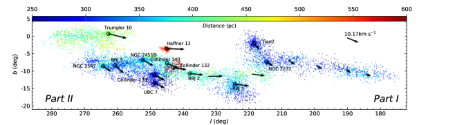
Figure 1: Spatial distribution ($l$-$b$) of the member candidates (color-coded with distance as represented in the color bar). The arrows over structures illustrate the average tangential velocities of stars in localized regions, while the arrow in the top-right corner marks the mean tangential velocity ($v_{l}=-9.47$ km $\rm s^{-1}$, $v_{b}=-3.72$ km $\rm s^{-1}$) of the whole structure. The lengths of the arrows are scaled with respect to the total tangential velocity of the whole structure (Parts I and II). All velocities are given with respect to the LSR.

3.2 Spatial Distribution

Figure 1 displays the distribution of the member candidates in the $l-b$ projected space. Each candidate is color-coded by distance. The black arrow in the top-right corner illustrates the average tangential velocity ($v_{l}=-9.47$ km $\rm s^{-1}$, $v_{b}=-3.72$ km $\rm s^{-1}$) of the whole sample. The remaining arrows display the average tangential velocities of localized regions. The arrow length corresponds to the value of velocity.

Figure 2 displays the spatial distribution of the member candidates in the Cartesian coordinates $(X,Y,Z)$ for Part I (black dots) and Part II (gray dots), respectively. Both the length (in the $X$-direction ) and width (in the $Y$-direction) are around 500 pc, but the thickness (in the $Z$-direction) is just over 100 pc.

As shown in Figure 1 and 2, Parts I and II are well bridged except for Haffner 13 and Collinder 132. These two distant clusters are also not well bridged with the main structure as presented in BBJ20 (see their Figure 8).

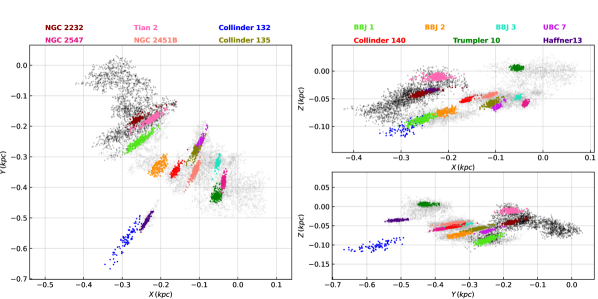
Figure 2: Spatial distribution of the member candidates in Cartesian coordinates $(X,Y,Z)$. The candidates in Parts I and II are shown with the black and gray dots, respectively. The 13 open clusters are color-coded as specified in the legend located above the figure. The coordinates of the Sun are $(X,Y,Z)=(0.0,0.0,0.0)$ kpc.

3.3 Open clusters

We identify 13 known open clusters in total (as shown in Figures 1$-$3). Part I includes NGC 2232 and Tian 2 (T20), and Part II includes Trumpler 10, Haffner 13, NGC 2547, NGC 2451B, Collinder 132, Collinder 135, Collinder 140, UBC 7, BBJ 1, BBJ 2, and BBJ 3 (BBJ20). These clusters are displayed with different colors in Figures 2 and 3. In Figure 2, the distribution of the clusters clearly shows a substantial elongation effect along the line of sight. This is induced by the deduced distances from inverse parallaxes (i.e., $d=1000\omega^{-1}$ (pc)). Comparing with BBJ20, we find finer sub-structures in our Part II region. For example, the clearly distinguishable physical pair of open clusters (Kovaleva et al., 2020), i.e., Collinder 135 and UBC 7 (see Figure 1). In addition to this pair, Tian 2 and NGC 2232 show characteristics of a physical pair according to their physical parameters, which will be further discussed in Section 4.

We roughly select the member candidates from the sample in Parts I and II for the 13 open clusters according to their coordinates, i.e., $(l-l_{0})^{2}+(b-b_{0})^{2}<{\epsilon_{0}}^{2}$. The central coordinate ($l_{0}$, $b_{0}$) is specified in Table 1 for each cluster, and the angular radius ($\epsilon_{0}$) is empirically chosen to be 1.0°$-$2.0° for each individual cluster. Thus, we obtain 304, 213, 249, 148, 291, 260, 104, 282, 137, 183, 344, 184, and 88 member candidates for NGC 2232, Tian 2, Trumpler 10, Haffner 13, NGC 2547, NGC 2451B, Collinder 132, Collinder 135, Collonder 140, UBC 7, BBJ 1, BBJ 2, and BBJ 3, respectively.

In Figure 3, the open clusters present different groups in the tangential velocity space ($v_{l}-v_{b}$). According to the patterns in velocity, we define five groups, namely, Trumpler 10 and its surrounding stars as Group I, Collinder 132, BBJ 1, BBJ 2, and their surrounding stars as Group II, NGC 2547, NGC 2451B, BBJ 3, Collinder 135, UBC 7, Collinder 140, and their surrounding stars as Group III, and Tian 2, NGC 2232, and its long tail as Group IV. Haffner 13 is relatively isolated in both the 3D spatial distribution (the indigo dots in Figure 2) and the tangential velocity distribution (the indigo dots in Figure 3). Therefore, Haffner 13 and its surrounding stars are labeled as Group V. We will investigate the 3D expansion rate for each group in Section 4.5.

4 Population Properties

We have 2694 and 9615 member candidates which can be used to analyze the statistical properties for Parts I and II, respectively.

4.1 Kinematics

Over half of the identified open clusters are clearly distinguishable in $v_{l}-v_{b}$, as shown in Figure 3, except for BBJ 1, BBJ 2, and Collinder 132 in Group II and Collinder 140 and Collinder 135 in Group III. Notably, the two physical pairs, Collinder 135 (olive) and UBC 7 (magenta) in Group III and Tian 2 (hot pink) and NGC 2232 (dark red) in Group IV, are clearly separated in tangential velocity space.

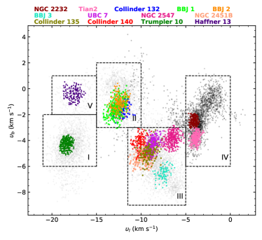
Figure 3: Distribution of tangential motions ($v_{l}-v_{b}$) for member stars of Parts I (black) and II (gray). The 13 open clusters are characterized by different patterns in velocity. Accordingly, we divide our sample into five groups. All velocities are with respect to the LSR. The color-coding is the same as in Figure 2.

Among the candidates in Part I, only 272 stars have radial velocities, of which 111 stars from Gaia, 23 stars from APOGEE DR14, 22 stars from LAMOST MRS (11 stars with Gaia’s $R_{V}$) and 104 stars from LAMOST LRS (38 stars with Gaia’s $R_{V}$), 12 stars from GALAH DR3 (7 stars with Gaia’s $R_{V}$). Among the candidates in Part II, only 734 stars have radial velocities, of which 681 stars from Gaia, 3 stars from RAVE (2 stars with Gaia’s $R_{V}$), 48 stars from GALAH DR3 (30 stars with Gaia’s $R_{V}$) and 2 stars from APOGEE DR14. For those stars that have been observed by multiple surveys, we use the median values as their observed radial velocities.

Figure 4 displays the 3D ($U,V,W$) velocity distributions for Part I (red) and Part II (blue) in the Cartesian coordinate, mainly for the four groups, i.e., Group I$-$IV (Group V only has 7 radial velocity available). The mean and rms of velocity components $(U,V,W)$ are $(-11.18\pm 4.60,-1.07\pm 3.04,-3.62\pm 1.10)$ km $\rm s^{-1}$ for Part I and $(-11.05\pm 6.88,-0.35\pm 6.41,-4.42\pm 1.47)$ km $\rm s^{-1}$ for Part II. It indicates that the 3D velocity of Part I is highly consistent with that of Part II. The outliers in the three sub-panels are likely peculiar members that have unresolved partners or high rotational speeds.

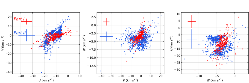
Figure 4: Distributions of the 3D $(U,V,W)$ velocities of the member candidates with $R_{V}$ in Part I (red) and Part II (blue). The 3D components $(U,V,W)$ for each candidate have been corrected for the solar peculiar velocity. The mean and rms of the velocity components are $(-11.18\pm 4.60,-1.07\pm 3.04,-3.62\pm 1.10)$ km $\rm s^{-1}$ for Part I and $(-11.05\pm 6.88,-0.35\pm 6.41,-4.42\pm 1.47)$ km $\rm s^{-1}$ for Part II. The error bars in the top-left corner of each panel mark the rms of the 3D velocity components for Part I (red) and Part II (blue).

In Figure 5, we show the variation of radial velocity $R_{V}$ along Galactic longitude $l$ for both Parts I and II. The radial velocities from different surveys are color-coded. For Part I, the radial velocities do not significantly change with Galactic longitude. For Part II, however, it seems that the radial velocities are inversely proportional to Galactic longitude. The average $R_{V}$ with uncertainty is $24.8\pm 0.3$ km $\rm s^{-1}$ for Part I, which is systematically about $7$ km $\rm s^{-1}$ faster than that in Part II ($17.7\,\pm 0.2$ km $\rm s^{-1}$), as shown in the histogram of $R_{V}$ in the right panel of Figure 6 (red for Part I, and blue for Part II). The distance from the Sun of the member candidates in Part II are on average 67 pc more distant than Part I (left panel of Figure 6).

We summarize the average velocities and distances for the 13 open clusters in Table 1.

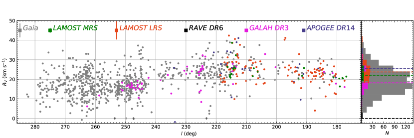
Figure 5: Distribution of the observed $R_{V}$ for all member candidates along Galactic longitude $l$. The $R_{V}$ are obtained from the multiple surveys (color-coded as specified in the legend). The error bars on each marker in the legend (top of the main panel) represent the average uncertainties of $R_{V}$ from the different surveys. The histograms of $R_{V}$ are displayed in the right sub-panel. The average values are marked with dashed lines. The color-coding is the same as the main panel.

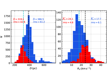
Figure 6: Histograms of distance from the Sun (left panel) and observed radial velocity (right panel) for member candidates from Part I (red) and Part II (blue). The minor peak at $d\sim 570$ pc in the left panel is mainly due to the presence of Haffner 13 and Collinder 132.

4.2 Chemistry and Surface Rotation

Figure 7 displays the variation of metallicity [Fe/H] (taken from various surveys) along Galactic longitude $l$ for member candidates. Specifically, we show 20 stars (red) from LAMOST MRS, 105 stars (green) from LAMOST LRS, 11 stars (dark slate blue) from Apogee DR14, and 58 stars (magenta) from Galah DR3. As shown in the figure, [Fe/H] spans a range of values between $-1.0$ dex and $0.25$ dex. The sample average from each survey is near solar ([Fe/H]$\sim 0$ dex), as shown by the histograms in the right sub-panel. Considering that the Snake is much younger than our Sun, we prefer to use $Z=0.02$ (slightly larger than the solar value of $Z_{\odot}=0.015$) in the following discussion.

The average and rms [Fe/H] for the whole sample are $-0.024$ dex and $0.130$ dex, respectively. The two black dashed horizontal lines mark the locations of $\pm\,3\sigma$. We consider the points beyond the two dashed lines as outliers. All the outliers are more metal poor than the mean metallicity of the Snake, particularly between $250\arcdeg<l<245\arcdeg$ where there seems to be a dip in Figure 7.

We investigate the relationship between [Fe/H] and absolute magnitude $M_{G}$ (top panel) and surface rotation $v\sin{i}$ (bottom panel) of member candidates in Figure 8. We find that all outliers in [Fe/H] are bright stars ($M_{G}<3.5$ mag) or those with high surface rotation ($v\sin{i}>50$ km $\rm s^{-1}$). This demonstrates that accurate metallicity measurements may be hampered by high stellar temperature or fast rotation.

Based on these results, we will use this data set to more thoroughly study stellar physics and the possible uncertainties involved in measuring stellar parameters such as surface rotation, effective temperature, and metallicity (Wang Fan et al. in preparation).

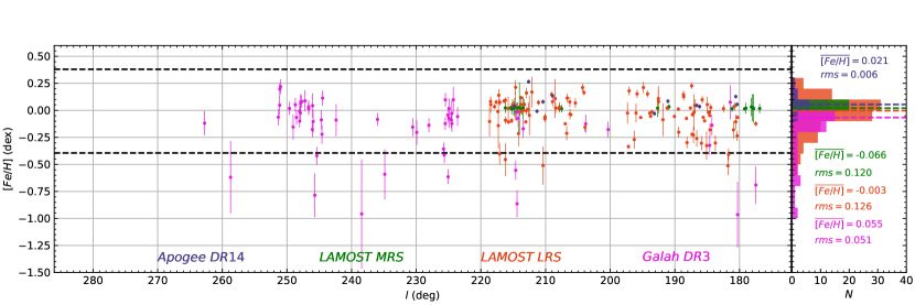
Figure 7: Distribution of [Fe/H] along Galactic longitude $l$. The values of [Fe/H] are obtained from multiple catalogs (color-coded as specified in the legend). The average and rms of [Fe/H] are $-0.024\pm 0.130$ dex for all 202 available candidates. The two black dashed horizontal lines mark the locations of $\pm 3\sigma$ around the average metallicity in the left main panel. The histograms of [Fe/H] from the different surveys are displayed in the right sub-panel. The average values are marked with dashed lines, and specified with the color-coded text. The color-coding is the same as Figure 5.

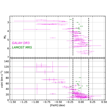
Figure 8: Comparison of [Fe/H] with absolute magnitude $M_{G}$ (top panel) and surface rotational velocity vsini (bottom panel) from LAMOST MRS (green) and Galah DR3 (magenta). The black dashed vertical lines mark the locations of $\pm 3\sigma$ around the average metallicity ($\sigma\simeq 0.13$ dex, same as that in Figure 7).

4.3 Age and Mass

T20 measured the age of the Snake (formally only Part I) using two different approaches: one based on isochrone fitting (Liu & Pang, 2019); and another using the Turn-On (Cignoni et al., 2010). Both methods give an age of 30$-$40 Myr for the Snake. Binks et al. (2021) measured an age of 38$\pm$3 Myr through the lithium depletion boundary for the open cluster NGC 2232, which is one of the most important components of the Snake. Therefore, we firmly believe that the Snake is 30$-$40 Myr old. In the following, we use an age of 34 Myr, which is the best fit value in T20, for both Parts I and II.

Figure 9 displays the CMDs of the member candidates in Part I (red dots) and Part II (blue dots) with three isochrones, i.e., 34 Myr (black solid curve), 5 Myr (green solid curve), and 120 Myr (green dashed curve). All three isochrones are from PARSEC (Bressan et al., 2012; Chen et al., 2014, 2015; Tang et al., 2014; Marigo et al., 2017) CMD 3.1 with metallicity $Z=0.02$. As shown in the figure, Parts I and II have nearly the same distribution in the CMD, which demonstrates that Parts I and II are of similar stellar population and very likely one sizable stellar structure which probably originated from the same GMC. We notice that the 34 Myr isochrone well-matches the observed CMDs for the bright stars, but in the faint end, the isochrone is not perfectly consistent with the observed distribution, particularly for the PMS stars with $M_{G}\gtrsim 9$ mag. This phenomenon was also seen by Li et al. (2020). This discrepancy is not likely due to the effect of extinction coefficients which should depend on spectral type (Chen et al., 2019); accounting for such a discrepancy requires an extinction of $A_{V}>2$ mag. Most of our sample stars are closer than 400 pc to the Sun (see Figure 6), which is not likely to have such a large extinction value. Given that stars with $M_{G}\gtrsim 9$ mag in our sample have a stellar mass $\lesssim 0.5$ $M_{\odot}$ and $T_{\rm eff}\lesssim 3200$ K, we argue that atmospheric models and PMS stellar evolutionary models of very low mass stars at low temperature need to be further improved. We also find that the sequence of Part I is slightly over that of Part II. This indicates that the stars in Part II are probably born a few Myr before those in Part I if the extinction values are calibrated correctly for both Parts. Slight differences in age are consistent with the differences in distance and proper motion detected in the member candidates of the Snake (Section 4.1).

Figure 10 illustrates the CMDs for the 13 open clusters (color-coded). The gray dots in the two left most panels in the upper row are the 2694 member candidates of Part I, while the gray dots in the remaining ten panels are the 9615 member candidates of Part II. The black curve in each panel is the 34 Myr isochrone. The CMD of each open cluster well traces the locus of the gray dots, and basically matches the isochrone (black curve), except for the Trumpler 10. Such discrepancy indicates that Trumpler 10 is slightly older than the other open clusters, its age being 40$-$50 Myr. Compared to previous studies estimating the age of Trumpler 10, our estimated age is most similar to Bossini et al. (2019, 45 Myr), and older than the ages of Kharchenko et al. (2013, 24 Myr) and Dias et al. (2002, 35 Myr). Besides Trumpler 10, all remaining open clusters have the same age, consistent with the estimated age of the Snake by T20, i.e., 30$-$40 Myr.

Based on the best fit isochrone, i.e., a 34 Myr isochrone, we estimate the stellar mass for each member candidate, and find that the new results from both Parts I and II support the claims about the mass distribution presented by T20, i.e., more than 84.0% of the members do not pass the TOn point ($G_{\mathrm{BP}}-G_{\mathrm{RP}}<1.0$ mag) and enter the MS stage, and most of the members have masses with $M<1.0\,\mathrm{M}_{\odot}$. Using the initial mass function of Kroupa et al. (2001), we roughly obtain a mass of $\sim 2500\,\mathrm{M}_{\odot}$ ($\sim 8000\,\mathrm{M}_{\odot}$) for Part I (Part II). Therefore, the total mass of the Snake should be larger than 10,000 $\mathrm{M}_{\odot}$.

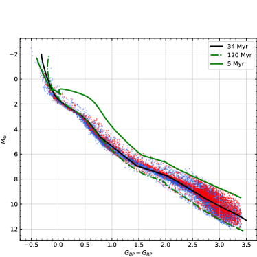
Figure 9: CMDs of the 2694 member candidates in Part I (red dots), the 9615 member candidates in Part II (blue dots). The black solid curve is the isochrone with an age of 34 Myr from T20. The other two isochrones are used to remove outliers with ages younger than 5 Myr (green solid curve) and 120 Myr (green dot-dashed curve) from the member candidates. All the isochrones are with Z = 0.02. The ages of both Parts I and II are 30$-$40 Myr, although Part I seems to be few Myrs younger than Part II.

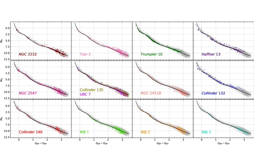
Figure 10: CMDs for the 13 open clusters (same color-coding as in Figures 2 and 3) of Parts I and II. The gray dots in the upper most row far left two panels and the remaining ten panels are the full sample of 2694 and 9615 member candidates of Parts I and II, respectively. The isochrones in all panels are of the same age (34 Myr) and $Z=0.02$. Trumpler 10 seems to be older than the other open clusters, which suggests an age of $40-50$ Myr. The two clusters of the physical pair (i.e., Collinder 135 and UBC 7) with exactly same age are displayed in the same panel. According to the CMDs, Tian 2 and NGC 2232 of Part I are probably also a physical pair.

4.4 Orbits and Integrals of motion for the open clusters

Most of open clusters include at least 10 member candidates with $R_{V}$, except for Haffner 13, Collinder 132 and BBJ 1 which only have 5, 6 and 8 members with $R_{V}$, respectively. We therefore have a sufficient number of open cluster member stars to calculate the central position ($l_{0}$, $b_{0}$) and the median value of $R_{V}$, proper motion, distance from the Sun, and $Z$-component of angular momentum ($L_{Z}$) for each cluster. We use the potential model of Bovy (2015) and the 6D phase information to calculate the orbits and total energy $E$ for the 13 open clusters. Figure 11 shows the color-coded orbits in the $R-Z$ space (left panel) and integrals of motion $E-L_{Z}$ (right panel) for the 13 open clusters.

In the left panel, each orbit includes three parts: (1) a black dot or filled square that is the current location of the cluster; (2) the solid curve which is the past orbit over the last 40 Myr; and (3) the dashed curve which is the future orbit over the next 50 Myr. It looks that in the past most of the open clusters were physically closer together compared to their present locations, and move away from each other in the future. This indicates that the whole structure is expending. Trumpler 10 and Haffner 13 present slightly different orbits compared to the other clusters.

In the right panel, Tian 2 and NGC 2232 in Part I and most components of Part II are assembled together and almost indistinguishable. This suggests that Parts I and II have considerably similar integrals of motion which demonstrates that Part I and most components of Part II are very likely one single unified structure. It worth noting that, Trumpler 10 and Haffner 13 which locate in the lower left part of the figure, are similar to each other but with different integrals of motion from most of the other clusters of Part II. Interestingly, BBJ 1 is also slightly isolated from the majority of clusters in Part II. There are two possible reasons: i) the integrals of motion of BBJ 1 are calculated only from 8 member candidates with radial velocities, the sample is sparse thus harm the significant level of its statistics. ii) some local regions including BBJ 1, Trumpler 10 and Haffner 13 probably experienced some unknown perturbations after they were formed.

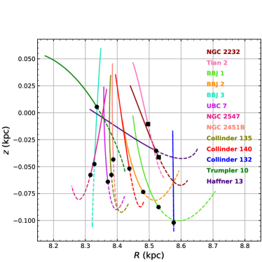
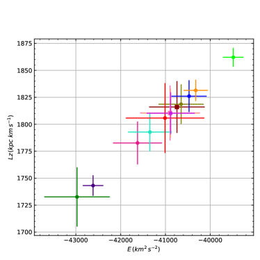
Figure 11: Left panel: Orbits of the 13 open clusters. The orbital parameters of each open cluster are the median values of its member candidates with $R_{V}$. Each orbit includes three parts:current positions (Part I: black filled squares, Part II: black dots), past orbits 40 Myr ago (solid curve), and future orbits 50 Myr later (dashed curve). Right panel: Distribution of the 13 open clusters in the integrals of motion ($L_{Z}$ and $E$) space. The filled squares (Part I) or dots (Part II) with error bars illustrate the median and rms values of $L_{Z}$ and $E$ of the member candidates with $R_{v}$ in the clusters. The color-coding is the same as in Figures 2, 3, and 10.

4.5 3D expansion rates

The orbits (Section 4.4) of the 13 open clusters demonstrate that the whole structure is expanding. In this section, we illustrate how localized regions (e.g., open clusters) expand. In Section 3.3, we divided the whole structure into 5 groups, and obtained the 6D phase information for some group members, i.e., 196, 159, 369, 264, and 7 stars with radial velocities in Groups I$-$V, respectively. In the following, we will use these stars to explore the 3D kinematics of Group I-IV. Because Group V only includes 7 stars with radial velocities, it is difficult to statistically study. We therefore do not calculate the expansion rate for Group V. We divide the member candidates of each group into 5 bins in the $X$-, $Y$-, and $Z$-directions, respectively. We consider the stars which are beyond $\pm 3\sigma$ of the corresponding velocities as outliers in each bin, and remove the outliers before the statistical analysis.

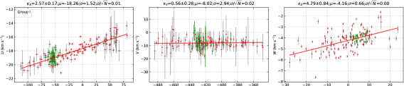
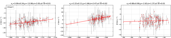
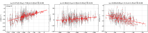
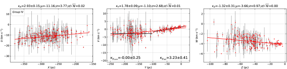
Figure 12: 3D velocities ($U,V,W$) as functions of 3D positions ($X,Y,Z$) for stars (red dots) in Group I$-$IV. The solid lines show the best fit linear relationships between the plotted quantities. The best fitting slope $\kappa$ with its uncertainty ($\times 10^{-2}$km $\rm s^{-1}$$\rm pc^{-1}$) and mean velocity $\mu$ (km $\rm s^{-1}$) with its standard deviation $\sigma$ (km $\rm s^{-1}$) and statistical uncertainty $\sigma/\sqrt{N}$ (km $\rm s^{-1}$) are noted above each panel. The green dots are the member candidates of Trumpler 10. If the groups are not expanding we expect slopes of zero, while if they are expanding we expect a positive slope (a negative slope implies a sign of contraction along the corresponding axis). Interestingly, Group IV presents two clear modes in the relationship between $Y$ and $V$ (lowest row, middle panel). The two clusters in the core (i.e., Tian 2 and NGC 2232 of Part I) show neither sign of expansion nor contraction ($\kappa_{Y_{\mathrm{core}}}\simeq 0.0\times 10^{-2}$km $\rm s^{-1}$$\rm pc^{-1}$) at $Y<-100$ pc; while the tail at $Y>-100$ pc clearly shows signs of expansion ($\kappa_{Y_{\mathrm{tail}}}\simeq 3.2\times 10^{-2}$km $\rm s^{-1}$$\rm pc^{-1}$), as shown by the two black regression lines (lowest row, middle column panel). Group III presents a significant sign of contraction in the $Z$-direction ($\kappa_{Z}\simeq-8.0\times 10^{-2}$km $\rm s^{-1}$$\rm pc^{-1}$). All slopes are summarized in Table 1.

Figure 12 displays the 3D kinematical variations along the 3D configuration space of the member candidates of Groups I$-$IV (upper to lower rows, respectively). The panels show $X-U$ (first column), $Y-V$ (second column), and $Z-W$ (third column). All four groups present significantly linear correlation between $X$ and $U$ with almost the same slope (i.e., $\kappa_{X}\simeq 3.0\times 10^{-2}$km $\rm s^{-1}$$\rm pc^{-1}$). This indicates that all of the four groups are expanding in the $X$-direction. According to the empirical relationship between the slope $\kappa$ and the expansion age, i.e., $\tau=(\gamma\kappa)^{-1}$ (where $\gamma$ = 1.0227 is the conversion factor from km $\rm s^{-1}$ to pc Myr^-1 (Blaauw, 1964; Wright & Mamajek, 2018)), $\kappa_{X}\simeq 3.0\times 10^{-2}$km $\rm s^{-1}$$\rm pc^{-1}$ signifies that the expansion age is around 33 Myr, which is highly consistent with the age of the Snake ($34$ Myr).

In the phase space $Y-V$, Group II and III present significant expansion similar to the phase space $X-U$; the values of $\kappa_{Y}$ are $2.22\pm 0.11$ (for Group II) and $2.38\pm 0.11$ (for Group III) $\times 10^{-2}$km $\rm s^{-1}$$\rm pc^{-1}$. Group I does not show a sign of expansion in the $Y$-direction ($\kappa_{Y}\simeq 0.56\pm 0.28\times 10^{-2}$km $\rm s^{-1}$$\rm pc^{-1}$). Interestingly, Collinder 132 is far from BBJ 1 and BBJ 2 in Group II, but its expansion rate (the five points at $Y<-500$ pc) seems to be well matched with the other Group II members. Group IV displays two clear modes in the relationship between $Y$ and $V$: the two clusters (i.e., Tian 2 and NGC 2232) show no sign of expanding or contraction (i.e., $\kappa_{Y}\simeq 0.0\pm 0.25\times 10^{-2}$km $\rm s^{-1}$$\rm pc^{-1}$) at $\rm Y<-100$ pc; while the tail ($\rm Y>-100$ pc) clearly shows signs of expanding ($\kappa_{Y}\simeq 3.2\pm 0.41\times 10^{-2}$km $\rm s^{-1}$$\rm pc^{-1}$), as shown by the two black lines (fourth row from the top, middle panel).

In the phase space $Z-W$, only Group I displays a sign of expansion ($\kappa_{Z}\simeq 4.79\pm 0.84\times 10^{-2}$km $\rm s^{-1}$$\rm pc^{-1}$). Strangely, Group III exhibits a strong sign of contraction in the $Z$-direction ($\kappa_{Z}\simeq-8.0\pm 0.65\times 10^{-2}$km $\rm s^{-1}$$\rm pc^{-1}$). This phenomenon was also noted by CG19b who measured a slope of $\kappa_{Z}\simeq-4.49\pm 0.37\times 10^{-2}$km $\rm s^{-1}$$\rm pc^{-1}$. Group II and IV do not display any significant signs of expansion or contraction.

Taking Trumpler 10 in Group I as an example, we investigate how the elongation effect along the line of sight as induced by inverting parallax (such that distances are $1000\omega^{-1}$ (pc)) affects the calculated expansion rate of the cluster. As shown by the green dots in Figure 12, the elongation effect mainly increases the uncertainty of velocity components in a limited region, but does not significantly affect the expansion rate.

The slopes for the four groups are summarized in Table 1.

4.6 Gas Environment

To investigate the relationship between the Snake and its surrounding gas environment, Figure 13 illustrates the overlapping distributions of the member candidates of the Snake and ¹²CO integrated intensity map in the velocity range from between $-$14 and 25 km $\rm s^{-1}$ in $l-b$ (top panel) and $l-R_{V,\mathrm{LSR}}$ (bottom panel). The ¹²CO data are taken from Dame et al. (2001), and the velocity range is chosen in accordance with the radial velocity range of the member candidates. Radial velocities of both the member candidates and the gas are with respect to the LRS. It seems that most of the components are not associated with the ¹²CO molecular cloud, which is expected since the gas has already likely dispersed in the past 30$-$40 Myr.

In Figure 13, the candidate members in Trumpler 10 seem to show a spatial and kinematic correlation with the ¹²CO molecular gas in their localized region. However, given that Trumpler 10 has an age of $\sim$40$-$50 Myr and the molecular cloud may not have remained present for so long (Hartmann et al., 2001), Trumpler 10 is very unlikely associated with the ¹²CO molecular cloud. Actually, the ¹²CO molecular cloud shown in the region of Trumpler 10 is the Vela molecular cloud (Murphy & May, 1991) with a distance of $\sim 870-970$ pc (Zucker et al., 2020). Thus, there is no physical association between Trumpler 10 and the Vela molecular cloud.

The Vela supernova remnant (Vela SNR), one of the closest SNRs to us (287${}^{+19}_{-17}$ pc, Dodson et al. 2003), is located in the sky region nearby Trumpler 10, as shown by the dashed circle in Figure 13. The Vela SNR interacts with its surrounding structures, e.g., the IRAS Vela Shell (IVS) which a ring-like structure discovered in far-infrared images by Sahu (1992) and the massive binary system $\gamma^{2}$ Velorum ($336^{+8}_{-7}$ pc, North et al. 2007). As modeled by Sushch et al. (2011), the IVS is the result of the stellar-wind bubble of $\gamma^{2}$ Velorum, and the observed asymmetry of the Vela SNR is due to the envelope of the Vela SNR physically meeting with the IVS. Furthermore, CG19a proposed that the stellar feedback and supernovae which exploded in the 30 Myr old clusters swept the gas away and produced the IVS, and that the expansion of the IVS triggered a second burst of star formation (e.g., $\gamma^{2}$ Velorum) approximately 10 Myr ago, as shown in their Figure 9. Our results suggest that Trumpler 10 seems unlikely to have participated in such a joint evolutionary process, since its distance is around 430 pc (see Table 1), which is much larger than that of the Vela SNR. However, the nearby clusters (e.g., NGC 2547, BBJ 3, and NGC 2451B) have very similar distances with the Vela SNR. They are probably associated with the Vela SNR.

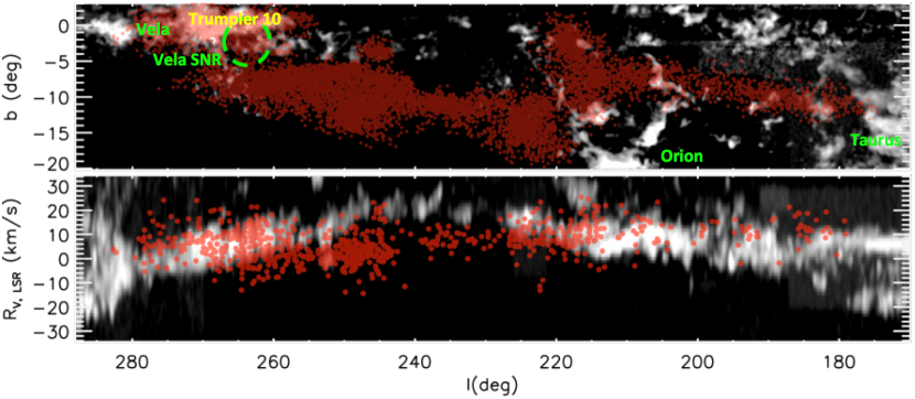
Figure 13: Distribution of the member candidates (red filled circles) of the Snake and CO gas (white) integrated over the velocity range between $-$14 and 25 km $\rm s^{-1}$ chosen according to the $R_{V,\mathrm{LSR}}$ range of the stars in the panels of $l-b$ (top panel) and $l-R_{V,\mathrm{LSR}}$ (bottom panel). The radial velocities of both the member candidates and gas are with respect to the LSR. The green dashed circle displays the location of the Vela supernova remnant (Vela SNR).

5 Discussion

In this section, we detail the likely formation scenario for the whole system, the Snake and its surrounding territory, and then briefly compare with other works in the literature.

5.1 Origin of the structures

We have investigated the properties of the member candidates for Parts I and II. In the perspective of spatial distributions, Parts I and II are well bridged, except for Haffner 13 and Collinder 132, which are relatively further than the other components. Parts I and II have nearly the same ages (i.e., $30-40$ Myr), even though Part II appears a few Myr older than Part I in the CMDs. Meanwhile, Trumpler 10 appears to be around 10 Myr older than the other parts. Considering integrals of motion, Part I has considerably similar $L_{z}$ and $E$ with most components of Part II. We do not detect significant differences in the metallicities of the two parts. With these in mind, we propose that Parts I and II are very likely born from the same environment, and belong to one sizable structure, but exhibit different formation and evolution history in some localized regions.

Though Haffner 13 and Collinder 132 are not well bridged with other components in Part II, and Haffner 13, Trumpler 10, and BBJ 1 present slightly different integrals of motion from the remaining components of Part II, we argue that the four clusters most likely belong to the whole structure of Part II, as claimed by BBJ20, or at lease were born from very similar environments in a very similar epoch, because the clusters share similar ages and metalicities with the other components of Part II.

In T20, we have basically ruled out the formation channel of tidal tails for such a sizable structure. The population is so young (only 30$-$40 Myr) that it cannot be well explained with the classical theory of tidal tails (Kharchenko et al., 2009; Jerabkova et al., 2019, 2021). The reasonable explanation is that the Snake is a hierarchically primordial structure, probably formed from a filamentary GMC. Gravitationally bound stellar clusters in this structure arise naturally at high local density regions, while unbound associations form in situ at low density regions. Therefore, the most probable scenario is like this: the older open cluster (e.g., Trumpler 10) was firstly born in the GMC around 40$-$50 Myr ago, and then the filamentary sub-structures in Part II including the 10 open clusters (e.g., a physical pair of Collinder 135 and UBC 7, etc.) were formed around 10 Myr later. After a few Myrs, the sub-structures in Part I including another physical pair of open clusters (i.e., Tian 2 and NGC 2232) were formed. During the Snake’s evolution, stellar feedback and supernovae of massive OB stars that exploded in the old (30$-$40 Myr) clusters may have produced a central cavity and shell, e.g., IVS (Sahu, 1992), and triggered a second burst of star formation (e.g., the 3$-$4 Myr binary system $\gamma^{2}$ Velorum, Jeffries et al., 2009) $\sim$10 Myr ago (CG19a). In addition, Tutukov et al. (2020) proposed that the snake-like or stream-like stellar structures possibly formed due to the decay of star clusters and OB associations.

The whole structure is expanding, as well as localized regions such as the open clusters, particularly in the $X$-direction. The expansion should not be due to the stellar winds from the massive OB stars, but caused by an event that took place before the stellar members formed, because the entire Snake is expanding, as discussed in CG19a.

5.2 Comparison with other works

BBJ20 applied the algorithm DBSCAN on Gaia DR2, and found a 260 pc wide and 35 Myr old filamentary structure nearby the Snake of T20. To study the relationship between the Snake and BBJ20’s structure, we build two samples (i.e., Parts I and II) to totally cover these two structures and run the coherent FOF algorithm as employed by T20 on the most recent data release of Gaia (Gaia EDR3). Using FOF we are able to recover the two structures and find that they are well bridged. Comparing with BBJ20, we find more fine sub-structures. For example, a physical pair of open clusters (Kovaleva et al., 2020), Collinder 135 and UBC 7, can be clearly distinguished in our newly combined structure (see Figure 1).

CG19b investigated the 3D expansion rates of the young population in the Vela-Puppis region. In their work, the authors divided the young population into seven sub-populations. The members of both their Population II and our Group I mostly belong to Trumpler 10. Their Population IV member mainly belong to Collinder 135, UBC 7, Collinder 140, NGC 2547, and NGC 2451B, while our Group III includes these plus an addition open cluster BBJ 3. Because the algorithms and the data (CG19b used Gaia DR2) are different, the final member candidates are slightly different. Taking Trumpler 10 as an example, CG19b find several sparse member candidates at $l<255$°(see their Figure 3), but we find no such members in this region. We cut the extra member candidates from the sample of CG19b, and carefully compare them with our sample. However, we find the extra candidates do not match well with our sample’s kinematics or CMD. Despite such differences in samples and sample selection between CG19b and our work, we find that the expansion rates are roughly consistent with each other (we compare our results in Table 1).

6 Summary and Conclusions

To search for all the stellar members belonging to the Snake and reveal its complete structure, we build two samples (i.e., Parts I and II) using Gaia EDR3 to investigate the relation between the Snake as defined by T20 and the filementary structure found by BBJ20. With the coherent FOF algorithm, we identified 2694 and 9615 member candidates from Parts I and II, respectively. Embedded within these member candidates are 13 open clusters. By combining spectroscopic data from multiple surveys, we investigate the comprehensive properties of these member candidates and find that they are very likely to belong to one sizable structure, because (1) most of the components are well bridged in configuration space (except for two distant clusters Collinder 132 and Haffner 13), (2) most of the components follow a single stellar population with an age of 30$-$40 Myr (except for the slightly older cluster Trumpler 10) and share solar metallicity, and (3) Part I presents considerably similar orbits and integrals of motion with most components of Part II.

The orbits of the 13 open clusters indicate that the whole structure is expanding. According to the tangential velocities $v_{l}$ and $v_{b}$, we divide our sample into five groups. We then calculate the 3D expansion rates for four of the five groups (Group V includes too few member candidates with $R_{V}$ to accurately measure its expansion rate). The expansion rates show that the four groups are expanding at a coherent rate ($\kappa_{X}\sim 3.0\,\rm\times 10^{-2}$ km $\rm s^{-1}$ $\rm pc^{-1}$) in the $X$-direction. The corresponding expansion age is perfectly consistent with the age of the Snake. Interestingly, Group III presents a significant sign of contraction in the $Z$-direction. The mechanism causing the expansion and contraction are still not clear.

In this work we rule out the formation channel of the Snake as due to a tidal tail. Our work shows that the Snake is most likely a hierarchically primordial structure, and probably formed from a filamentary GMC with different formation histories in several different localized regions. We propose the most likely formation scenario of the Snake is as follows. Trumpler 10 was first to be born in the GMC around 40$-$50 Myr ago, followed by the filamentary sub-structures in Part II including 10 open clusters (e.g., Collinder 135, UBC 7, etc), which formed around 10 Myr later. After another few Myrs, the sub-structures in Part I including Tian 2 and NGC 2232 formed.

Trumpler 10, Haffner 13, and BBJ 1 have slightly different integrals of motion ($L_{z}$ and $E$) from the other components of the Snake. This indicates that these localized regions probably experienced some type of dynamical perturbation after they were formed. During the Snake’s evolution, stellar feedback and the explosion of supernovae of massive OB stars in the old (30$-$50 Myr) clusters may have produced a central cavity and shell (e.g., IVS, Sahu, 1992), and trigger a second burst (e.g., the binary system $\gamma^{2}$ Velorum) of star formation $\sim$10 Myr ago (CG19a).

The Snake has more than ten thousand member candidates following a single stellar population (30$-$40 Myr old) and continuous mass function. Besides the massive O and B members, it also includes a number of lower-mass stars and PMS stars over hundreds of parsecs in our solar neighborhood. Therefore, it will provide us an ideal laboratory to study the history of stellar formation, environmental evolution, and stellar physics. For example, it is a good sample to study stellar binarity (El-Badry et al., 2019; Tian et al., 2020) in young populations, the surface rotation dichotomy (Sun et al., 2019), the initial mass function of low-mass stars (Hallakoun & Maoz, 2021), and so on. Also, it has great potential to reveal the relationship between young stellar populations and the spiral arms (Quillen et al., 2020; Hao et al., 2021), the rotating bar (Tian et al., 2017), and the vertical phase mixing (Antoja et al., 2018; Tian et al., 2018; Li, 2021). Moreover, it may provide some clues to understand the formation of some Galactic-scale structures, e.g., the Gould Belt (Poppel, 1997) and the Radcliffe Wave (Alves et al., 2020).

Table 1: The properties of the 13 open clusters included in Parts I and II.

Samp.

Cluster

$l_{0}$

$b_{0}$

$d$

$U$

$V$

$W$

${\mu_{l^{*}}}^{a}$

${\mu_{b}}^{a}$

$R_{V}$

Age

Gr.

$\kappa_{\rm X}$

$\kappa_{\rm Y}$

$\kappa_{\rm Z}$

($\arcdeg$)

pc

km $\rm s^{-1}$

mas $\rm yr^{-1}$

km $\rm s^{-1}$

Myr

$\rm 10^{-2}kms^{-1}pc^{-1}$

Part I

Tian 2

218.33

-2.12

$285.9\pm 0.3$

-8.0$\pm$0.9

-1.9$\pm$0.7

-4.0$\pm$0.1

-1.1$\pm$0.1

-7.6$\pm$0.1

$21.8\pm 1.1$

34

IV

2.93$\pm$0.15

1.78$\pm$0.09

-1.32$\pm$0.31

NGC 2232

214.42

-7.51

$319.2\pm 0.5$

-9.9$\pm$1.1

-2.6$\pm$0.9

-4.0$\pm$0.3

-0.6$\pm$0.1

-5.0$\pm$0.1

$24.7\pm 1.4$

34

Part II

Trum. 10

262.71

0.72

$433.9\pm 0.2$

-19.0$\pm$0.2

-8.1$\pm$0.7

-4.0$\pm$0.1

-12.9$\pm$0.1

-5.6$\pm$0.1

$21.7\pm 0.7$

40-50

I

2.57$\pm$0.17

0.56$\pm$0.28

4.79$\pm$0.84

${2.14\pm 0.19}^{b}$

${0.98\pm 0.57}^{b}$

${5.24\pm 0.19}^{b}$

Coll. 132

242.89

-9.04

$645.8\pm 1.1$

-15.7$\pm$0.9

-6.1$\pm$2.0

-3.0$\pm$0.2

-5.2$\pm$0.1

-2.1$\pm$0.1

$27.1\pm 2.1$

34

II

3.09$\pm$0.24

2.22$\pm$0.11

0.88$\pm$0.90

BBJ 1

224.26

-13.76

$368.5\pm 0.7$

-14.1$\pm$0.7

3.1$\pm$0.7

-2.8$\pm$0.4

-6.8$\pm$0.1

-2.8$\pm$0.1

$23.4\pm 0.9$

34

BBJ 2

238.17

-10.71

$393.7\pm 0.7$

-13.7$\pm$-0.4

0.6$\pm$0.3

-2.7$\pm$0.1

-8.0$\pm$0.1

-2.9$\pm$0.1

$21.9\pm 0.4$

34

BBJ 3

260.75

-8.36

$326.6\pm 0.6$

-7.4$\pm$0.1

0.4$\pm$0.7

-6.3$\pm$0.2

-9.9$\pm$0.1

-7.6$\pm$0.1

$14.2\pm 0.7$

34

III

3.27$\pm$0.15

2.38$\pm$0.11

-8.00$\pm$0.65

NGC 2547

264.42

-8.60

$386.0\pm 0.5$

-6.0$\pm$0.1

-0.4$\pm$0.6

-3.9$\pm$0.1

-8.2$\pm$0.1

-5.0$\pm$0.1

$13.6\pm 0.6$

34

${2.96\pm 0.14}^{b}$

${1.60\pm 0.36}^{b}$

-${4.49\pm 0.37}^{b}$

NGC 2451B

252.31

-6.81

$363.7\pm 0.6$

-9.4$\pm$0.3

0.7$\pm$0.7

-5.0$\pm$0.1

-8.9$\pm$0.1

-6.0$\pm$0.1

$16.6\pm 0.8$

34

Coll. 135

248.81

-11.03

$299.4\pm 0.3$

-8.4$\pm$0.2

2.3$\pm$0.4

-5.1$\pm$0.1

-10.0$\pm$0.1

-6.4$\pm$0.1

$16.1\pm 0.4$

34

Coll. 140

244.95

-7.77

$383.9\pm 0.8$

-11.8$\pm$0.6

-1.4$\pm$1.2

-4.6$\pm$0.2

-7.9$\pm$0.1

-5.0$\pm$0.1

$21.1\pm 1.4$

34

UBC 7

248.73

-13.51

$276.3\pm 0.3$

-8.3$\pm$0.2

1.4$\pm$0.5

-4.3$\pm$0.2

-10.5$\pm$0.1

-5.9$\pm$0.1

$16.9\pm 0.6$

34

Haffner 13

245.05

-3.60

$560.3\pm 1.5$

-23.7$\pm$0.6

-11.3$\pm$1.1

-1.5$\pm$0.4

-8.2$\pm$0.1

-2.5$\pm$0.1

$33.7\pm 1.2$

34

V

-

-

-

References

- Alves et al. (2020) Alves, J., Zucker, C., Goodman, A. A., et al. 2020, Nature, 578, 237, doi: 10.1038/s41586-019-1874-z
- Antoja et al. (2018) Antoja, T., Helmi, A., Romero-Gómez, M., et al. 2018, Nature, 561, 360, doi: 10.1038/s41586-018-0510-7
- Armstrong et al. (2018) Armstrong, J. J., Wright, N. J., & Jeffries, R. D. 2018, MNRAS, 480, L121, doi: 10.1093/mnrasl/sly137
- Armstrong et al. (2020) Armstrong, J. J., Wright, N. J., Jeffries, R. D., & Jackson, R. J. 2020, MNRAS, 494, 4794, doi: 10.1093/mnras/staa939
- Astropy Collaboration et al. (2013) Astropy Collaboration, Robitaille, T. P., Tollerud, E. J., et al. 2013, A&A, 558, A33, doi: 10.1051/0004-6361/201322068
- Beccari et al. (2020) Beccari, G., Boffin, H. M. J., & Jerabkova, T. 2020, MNRAS, 491, 2205, doi: 10.1093/mnras/stz3195
- Beccari et al. (2018) Beccari, G., Boffin, H. M. J., Jerabkova, T., et al. 2018, MNRAS, 481, L11, doi: 10.1093/mnrasl/sly144
- Behroozi et al. (2013) Behroozi, P. S., Wechsler, R. H., & Wu, H.-Y. 2013, ApJ, 762, 109, doi: 10.1088/0004-637X/762/2/109
- Binks et al. (2021) Binks, A. S., Jeffries, R. D., Jackson, R. J., et al. 2021, MNRAS, 505, 1280, doi: 10.1093/mnras/stab1351
- Blaauw (1964) Blaauw, A. 1964, ARA&A, 2, 213, doi: 10.1146/annurev.aa.02.090164.001241
- Bossini et al. (2019) Bossini, D., Vallenari, A., Bragaglia, A., et al. 2019, VizieR Online Data Catalog, J/A+A/623/A108
- Bovy (2015) Bovy, J. 2015, ApJS, 216, 29, doi: 10.1088/0067-0049/216/2/29
- Bressan et al. (2012) Bressan, A., Marigo, P., Girardi, L., et al. 2012, MNRAS, 427, 127, doi: 10.1111/j.1365-2966.2012.21948.x
- Buder et al. (2021) Buder, S., Sharma, S., Kos, J., et al. 2021, MNRAS, doi: 10.1093/mnras/stab1242
- Cantat-Gaudin et al. (2019a) Cantat-Gaudin, T., Mapelli, M., Balaguer-Núñez, L., et al. 2019a, A&A, 621, A115, doi: 10.1051/0004-6361/201834003
- Cantat-Gaudin et al. (2018) Cantat-Gaudin, T., Jordi, C., Vallenari, A., et al. 2018, A&A, 618, A93, doi: 10.1051/0004-6361/201833476
- Cantat-Gaudin et al. (2019b) Cantat-Gaudin, T., Jordi, C., Wright, N. J., et al. 2019b, A&A, 626, A17, doi: 10.1051/0004-6361/201834957
- Chen et al. (2020) Chen, B., D’Onghia, E., Alves, J., & Adamo, A. 2020, A&A, 643, A114, doi: 10.1051/0004-6361/201935955
- Chen et al. (2015) Chen, Y., Bressan, A., Girardi, L., et al. 2015, MNRAS, 452, 1068, doi: 10.1093/mnras/stv1281
- Chen et al. (2014) Chen, Y., Girardi, L., Bressan, A., et al. 2014, MNRAS, 444, 2525, doi: 10.1093/mnras/stu1605
- Chen et al. (2019) Chen, Y., Girardi, L., Fu, X., et al. 2019, A&A, 632, A105, doi: 10.1051/0004-6361/201936612
- Cignoni et al. (2010) Cignoni, M., Tosi, M., Sabbi, E., et al. 2010, ApJ, 712, L63, doi: 10.1088/2041-8205/712/1/L63
- Cui et al. (2012) Cui, X.-Q., Zhao, Y.-H., Chu, Y.-Q., et al. 2012, Research in Astronomy and Astrophysics, 12, 1197, doi: 10.1088/1674-4527/12/9/003
- Da Rio et al. (2016) Da Rio, N., Tan, J. C., Covey, K. R., et al. 2016, ApJ, 818, 59, doi: 10.3847/0004-637X/818/1/59
- Dame et al. (2001) Dame, T. M., Hartmann, D., & Thaddeus, P. 2001, ApJ, 547, 792, doi: 10.1086/318388
- de Zeeuw et al. (1999) de Zeeuw, P. T., Hoogerwerf, R., de Bruijne, J. H. J., Brown, A. G. A., & Blaauw, A. 1999, AJ, 117, 354, doi: 10.1086/300682
- Dias et al. (2002) Dias, W. S., Alessi, B. S., Moitinho, A., & Lépine, J. R. D. 2002, A&A, 389, 871, doi: 10.1051/0004-6361:20020668
- Dobbs (2013) Dobbs, C. 2013, Astronomy and Geophysics, 54, 5.24, doi: 10.1093/astrogeo/att165
- Dodson et al. (2003) Dodson, R., Legge, D., Reynolds, J. E., & McCulloch, P. M. 2003, ApJ, 596, 1137, doi: 10.1086/378089
- El-Badry et al. (2019) El-Badry, K., Rix, H.-W., Tian, H., Duchêne, G., & Moe, M. 2019, MNRAS, 489, 5822, doi: 10.1093/mnras/stz2480
- Fang et al. (2021) Fang, M., Kim, J. S., Pascucci, I., & Apai, D. 2021, ApJ, 908, 49, doi: 10.3847/1538-4357/abcec8
- Fang et al. (2013) Fang, M., Kim, J. S., van Boekel, R., et al. 2013, ApJS, 207, 5, doi: 10.1088/0067-0049/207/1/5
- Fang et al. (2009) Fang, M., van Boekel, R., Wang, W., et al. 2009, A&A, 504, 461, doi: 10.1051/0004-6361/200912468
- Fang et al. (2017) Fang, M., Kim, J. S., Pascucci, I., et al. 2017, AJ, 153, 188, doi: 10.3847/1538-3881/aa647b
- Franciosini et al. (2018) Franciosini, E., Sacco, G. G., Jeffries, R. D., et al. 2018, A&A, 616, L12, doi: 10.1051/0004-6361/201833815
- Gaia Collaboration et al. (2021) Gaia Collaboration, Brown, A. G. A., Vallenari, A., et al. 2021, A&A, 649, A1, doi: 10.1051/0004-6361/202039657
- Hallakoun & Maoz (2021) Hallakoun, N., & Maoz, D. 2021, MNRAS, doi: 10.1093/mnras/stab2145
- Hao et al. (2021) Hao, C. J., Xu, Y., Hou, L. G., et al. 2021, arXiv e-prints, arXiv:2107.06478. https://arxiv.org/abs/2107.06478
- Hartmann et al. (2001) Hartmann, L., Ballesteros-Paredes, J., & Bergin, E. A. 2001, ApJ, 562, 852, doi: 10.1086/323863
- Hillenbrand (1997) Hillenbrand, L. A. 1997, AJ, 113, 1733, doi: 10.1086/118389
- Hunter (2007) Hunter, J. D. 2007, Computing in Science and Engineering, 9, 90, doi: 10.1109/MCSE.2007.55
- Jeffries et al. (2009) Jeffries, R. D., Naylor, T., Walter, F. M., Pozzo, M. P., & Devey, C. R. 2009, MNRAS, 393, 538, doi: 10.1111/j.1365-2966.2008.14162.x
- Jerabkova et al. (2019) Jerabkova, T., Boffin, H. M. J., Beccari, G., & Anderson, R. I. 2019, MNRAS, 489, 4418, doi: 10.1093/mnras/stz2315
- Jerabkova et al. (2021) Jerabkova, T., Boffin, H. M. J., Beccari, G., et al. 2021, A&A, 647, A137, doi: 10.1051/0004-6361/202039949
- Kharchenko et al. (2009) Kharchenko, N. V., Berczik, P., Petrov, M. I., et al. 2009, A&A, 495, 807, doi: 10.1051/0004-6361/200810407
- Kharchenko et al. (2013) Kharchenko, N. V., Piskunov, A. E., Roeser, S., Schilbach, E., & Scholz, R. D. 2013, VizieR Online Data Catalog, J/A+A/558/A53
- Kos et al. (2019) Kos, J., Bland-Hawthorn, J., Asplund, M., et al. 2019, A&A, 631, A166, doi: 10.1051/0004-6361/201834710
- Kounkel & Covey (2019) Kounkel, M., & Covey, K. 2019, AJ, 158, 122, doi: 10.3847/1538-3881/ab339a
- Kounkel et al. (2018a) Kounkel, M., Covey, K., Suárez, G., et al. 2018a, AJ, 156, 84, doi: 10.3847/1538-3881/aad1f1
- Kounkel et al. (2018b) —. 2018b, The APOGEE-2 Survey of the Orion Star-forming Complex. II. Six-dimensional Structure, doi: 10.3847/1538-3881/aad1f1
- Kovaleva et al. (2020) Kovaleva, D. A., Ishchenko, M., Postnikova, E., et al. 2020, A&A, 642, L4, doi: 10.1051/0004-6361/202039215
- Kroupa et al. (2001) Kroupa, P., Aarseth, S., & Hurley, J. 2001, MNRAS, 321, 699, doi: 10.1046/j.1365-8711.2001.04050.x
- Li et al. (2020) Li, L., Shao, Z., Li, Z.-Z., et al. 2020, ApJ, 901, 49, doi: 10.3847/1538-4357/abaef3
- Li (2021) Li, Z.-Y. 2021, ApJ, 911, 107, doi: 10.3847/1538-4357/abea17
- Lindegren et al. (2018) Lindegren, L., Hernández, J., Bombrun, A., et al. 2018, A&A, 616, A2, doi: 10.1051/0004-6361/201832727
- Liu et al. (2020) Liu, C., Fu, J., Shi, J., et al. 2020, arXiv e-prints, arXiv:2005.07210. https://arxiv.org/abs/2005.07210
- Liu & Pang (2019) Liu, L., & Pang, X. 2019, ApJS, 245, 32, doi: 10.3847/1538-4365/ab530a
- Majewski et al. (2017) Majewski, S. R., Schiavon, R. P., Frinchaboy, P. M., et al. 2017, AJ, 154, 94, doi: 10.3847/1538-3881/aa784d
- Marigo et al. (2017) Marigo, P., Girardi, L., Bressan, A., et al. 2017, ApJ, 835, 77, doi: 10.3847/1538-4357/835/1/77
- Meingast et al. (2021) Meingast, S., Alves, J., & Rottensteiner, A. 2021, A&A, 645, A84, doi: 10.1051/0004-6361/202038610
- Murphy & May (1991) Murphy, D. C., & May, J. 1991, A&A, 247, 202
- Nidever et al. (2015) Nidever, D. L., Holtzman, J. A., Allende Prieto, C., et al. 2015, AJ, 150, 173, doi: 10.1088/0004-6256/150/6/173
- North et al. (2007) North, J. R., Tuthill, P. G., Tango, W. J., & Davis, J. 2007, MNRAS, 377, 415, doi: 10.1111/j.1365-2966.2007.11608.x
- Pang et al. (2021) Pang, X., Yu, Z., Tang, S.-Y., et al. 2021, arXiv e-prints, arXiv:2106.07658. https://arxiv.org/abs/2106.07658
- Poppel (1997) Poppel, W. 1997, Fund. Cosmic Phys., 18, 1
- Quillen et al. (2020) Quillen, A. C., Pettitt, A. R., Chakrabarti, S., et al. 2020, MNRAS, 499, 5623, doi: 10.1093/mnras/staa3189
- Sahu (1992) Sahu, M. S. 1992, PhD thesis, Kapteyn Institute, Postbus 800 9700 AV Groningen, The Netherlands
- Schneider & Elmegreen (1979) Schneider, S., & Elmegreen, B. G. 1979, ApJS, 41, 87, doi: 10.1086/190609
- Schönrich (2012) Schönrich, R. 2012, MNRAS, 427, 274, doi: 10.1111/j.1365-2966.2012.21631.x
- Soler et al. (2021) Soler, J. D., Beuther, H., Syed, J., et al. 2021, A&A, 651, L4, doi: 10.1051/0004-6361/202141327
- Steinmetz et al. (2020) Steinmetz, M., Matijevič, G., Enke, H., et al. 2020, AJ, 160, 82, doi: 10.3847/1538-3881/ab9ab9
- Su et al. (2015) Su, Y., Zhang, S., Shao, X., & Yang, J. 2015, ApJ, 811, 134, doi: 10.1088/0004-637X/811/2/134
- Sun et al. (2019) Sun, W., Li, C., Deng, L., & de Grijs, R. 2019, ApJ, 883, 182, doi: 10.3847/1538-4357/ab3cd0
- Sushch et al. (2011) Sushch, I., Hnatyk, B., & Neronov, A. 2011, A&A, 525, A154, doi: 10.1051/0004-6361/201015346
- Tang et al. (2014) Tang, J., Bressan, A., Rosenfield, P., et al. 2014, MNRAS, 445, 4287, doi: 10.1093/mnras/stu2029
- Taylor (2005) Taylor, M. B. 2005, in Astronomical Society of the Pacific Conference Series, Vol. 347, Astronomical Data Analysis Software and Systems XIV, ed. P. Shopbell, M. Britton, & R. Ebert, 29
- Tian (2017) Tian, H. 2017, PhD thesis, University of Groningen
- Tian (2020) Tian, H.-J. 2020, ApJ, 904, 196, doi: 10.3847/1538-4357/abbf4b
- Tian et al. (2020) Tian, H.-J., El-Badry, K., Rix, H.-W., & Gould, A. 2020, ApJS, 246, 4, doi: 10.3847/1538-4365/ab54c4
- Tian et al. (2014) Tian, H.-J., Liu, C., Hu, J.-Y., Xu, Y., & Chen, X.-L. 2014, A&A, 561, A142, doi: 10.1051/0004-6361/201322381
- Tian et al. (2018) Tian, H.-J., Liu, C., Wu, Y., Xiang, M.-S., & Zhang, Y. 2018, ApJ, 865, L19, doi: 10.3847/2041-8213/aae1f3
- Tian et al. (2015) Tian, H.-J., Liu, C., Carlin, J. L., et al. 2015, ApJ, 809, 145, doi: 10.1088/0004-637X/809/2/145
- Tian et al. (2017) Tian, H.-J., Liu, C., Wan, J.-C., et al. 2017, Research in Astronomy and Astrophysics, 17, 114, doi: 10.1088/1674-4527/17/11/114
- Tutukov et al. (2020) Tutukov, A. V., Sizova, M. D., & Vereshchagin, S. V. 2020, Astronomy Reports, 64, 827, doi: 10.1134/S106377292010008X
- van der Walt et al. (2011) van der Walt, S., Colbert, S. C., & Varoquaux, G. 2011, Computing in Science and Engineering, 13, 22, doi: 10.1109/MCSE.2011.37
- Wright & Mamajek (2018) Wright, N. J., & Mamajek, E. E. 2018, MNRAS, 476, 381, doi: 10.1093/mnras/sty207
- Zari et al. (2019) Zari, E., Brown, A. G. A., & de Zeeuw, P. T. 2019, A&A, 628, A123, doi: 10.1051/0004-6361/201935781
- Zhao et al. (2012) Zhao, G., Zhao, Y.-H., Chu, Y.-Q., Jing, Y.-P., & Deng, L.-C. 2012, Research in Astronomy and Astrophysics, 12, 723, doi: 10.1088/1674-4527/12/7/002
- Zucker et al. (2018) Zucker, C., Battersby, C., & Goodman, A. 2018, ApJ, 864, 153, doi: 10.3847/1538-4357/aacc66
- Zucker et al. (2020) Zucker, C., Speagle, J. S., Schlafly, E. F., et al. 2020, A&A, 633, A51, doi: 10.1051/0004-6361/201936145