On the asymptotics of the meromorphic 3D-index

Abstract.

In their recent work, Garoufalidis and Kashaev extended the 3D-index of an ideally triangulated 3-manifold with toroidal boundary to a well-defined topological invariant which takes the form of a meromorphic function of $2$ complex variables per boundary component and which depends additionally on a quantisation parameter $q$. In this paper, we study the asymptotics of this invariant as $q$ approaches 1, developing a conjectural asymptotic approximation in the form of a sum of contributions associated to certain flat $PSL(2,\mathbb{C})$-bundles on the manifold. Furthermore, we study the coefficients appearing in these contributions, which include the hyperbolic volume, the ‘1-loop invariant’ of Dimofte and Garoufalidis, as well as a new topological invariant of 3-manifolds with torus boundary, which we call the ‘beta invariant’. The technical heart of our analysis is the expression of the state-integral of the Garoufalidis–Kashaev invariant as an integral over a certain connected component of the space of circle-valued angle structures. To explain the topological significance of this component, we develop a theory connecting circle-valued angle structures to the obstruction theory for lifting a (boundary-parabolic) $PSL(2,\mathbb{C})$-representation of the fundamental group to a (boundary-unipotent) $SL(2,\mathbb{C})$-representation. We present strong theoretical and numerical evidence for the validity of our asymptotic approximations.

1. Introduction

The 3D-index is a fascinating invariant of ideal triangulations of oriented 3-manifolds with toroidal boundary which associates a $q$-series with integer coefficients to each first homology class of the boundary. It was originally obtained by Dimofte, Gaiotto and Gukov in a mathematical physics context from a certain superconformal field theory [DGG13, DGG14]. Garoufalidis provided an axiomatic formulation of the 3D-index and studied convergence of this invariant, which is only defined for some ideal triangulations [Ga16].

Although the physics predicts that the 3D-index should be a topological invariant, there is no a priori mathematical reason that this should be so. While the 3D-index is invariant under Pachner 2-3 moves on ideal triangulations (whenever it is defined on both sides of the move), it is not known whether all topological ideal triangulations on which the 3D-index is defined can be connected by such moves, so topological invariance does not follow. Nonetheless, Garoufalidis, Rubinstein, Segerman and the first named author showed in [GHRS15] that the 3D-index does indeed give a topological invariant in the special case of cusped hyperbolic 3-manifolds.

This paper concerns a certain extension of the 3D-index which was introduced by Garoufalidis and Kashaev [GK19] and which we will call the meromorphic 3D-index. The extension associates to every ideal triangulation of an oriented 3-manifold with toroidal boundary a meromorphic function which has 2 variables for every boundary component. The meromorphic 3D-index is invariant under all 2-3 Pachner moves, and is hence a topological invariant.

The meromorphic 3D-index is an extension of the $q$-series 3D-index in the following sense. In the case that the ideal triangulation has a strict angle structure, there is a Laurent expansion of the meromorphic 3D-index whose coefficients are the $q$-series appearing in the original 3D-index. Therefore, we can think of the meromorphic 3D-index as a kind of generating function for these $q$-series. In particular, the $q$-series 3D-index is a true topological invariant when restricted to ideal triangulations admitting strict angle structures.

The meromorphic 3D-index introduced in [GK19] depends on a complex parameter $q$ satisfying $0<|q|<1$. The main goal of this paper is to study the asymptotics of this invariant when $q\to 1$. More precisely, we express the meromorphic 3D-index in terms of a parameter $\hbar\in(-\infty,0)$ which determines a $q\in(0,1)$ by $q=e^{\hbar}$. The meromorphic 3D-index evaluated on the ideal triangulation $\mathcal{T}$ with a single torus boundary component is then denoted $\mathcal{I}_{\mathcal{T},(A_{\mu},A_{\lambda})}(\hbar)$ and is a meromorphic function of two complex variables $A_{\mu},A_{\lambda}$. These variables can be interpreted as the angle-holonomies, along the curves $\mu$ and $\lambda$, of a complexified angle structure on $\mathcal{T}$, in a sense that will be made more precise later.

Of particular interest is the behaviour of this invariant at the point $A_{\mu}=A_{\lambda}=0$, corresponding to trivial peripheral holonomies, since the value at this point does not depend on the choice of the curves $\mu$, $\lambda$. Moreover, in the case the manifold is hyperbolic, this point corresponds to an angle structure derived from the complete hyperbolic structure.

In this paper, we mostly focus on the case of a one-cusped hyperbolic manifold $M$ and study the asymptotic behaviour of the meromorphic 3D-index for $\hbar=-1/\kappa$, which corresponds to $q=\exp(-1/\kappa)$:

(1.1) $$\mathcal{I}_{M,(0,0)}(-1/\kappa),\quad\kappa>0,\quad\kappa\rightarrow\infty.$$

In Section 1.4, we provide a conjectural asymptotic approximation for the above quantity, in the form of a sum over conjugacy classes of irreducible, boundary-parabolic representations $\rho:\pi_{1}(M)\rightarrow PSL(2,\mathbb{C})$ with a certain fixed obstruction class to lifting the representation to $SL(2,\mathbb{C})$. Moreover, we will use heuristic saddle-point methods to develop explicit formulae for these contributions. Our asymptotic approximations show strong agreement with numerical experiments, which we describe in Section 10.

Although the overall picture is conjectural and based on a heuristic analysis, we will present many rigorous theorems about the various expressions that arise as coefficients in our asymptotic approximations. In particular, we expect some of these coefficients to be given by classical quantities, such as the volume of a representation and the Reidemeister torsion associated to its adjoint. Moreover, we use the total predicted contribution of boundary-parabolic real representations $\rho:\pi_{1}(M)\rightarrow PSL(2,\mathbb{R})$ to construct a new topological invariant, which we call the beta invariant. The beta invariant is defined in terms of state-integrals on ideal triangulations built from the Euler beta function and shown, in Section 9, to be fully invariant under Pachner 2-3 moves. Along the way, we study the cohomological obstruction classes to lifting boundary-parabolic $PSL(2,\mathbb{C})$-representations of $\pi_{1}(M)$ to boundary-unipotent $SL(2,\mathbb{C})$-representations and develop a theory to explain their relationship to circle-values angle structures on ideal triangulations.

1.1. A sketch of the meromorphic 3D-index

Here we’ll give a brief sketch of the construction of meromorphic 3D-index in the special case of a 3-manifold with a single torus boundary component. Section 4 below gives a detailed review.

To be precise, we need to consider two cases: the case when the triangulation admits a strict angle structure, and the case when it does not. (A strict angle structure is an assignment of strictly positive real numbers to normal quadrilateral types which sums to $\pi$ in each tetrahedron and to $2\pi$ around each edge.)

In the case the triangulation does admit a strict angle structure, we will write down a state-integral expression which depends on the triangulation and a strict angle structure on it. The strict angle structure ensures convergence of the integral, but the value of the integral depends on the strict angle structure only through the peripheral angle-holonomies $A_{\mu}$ and $A_{\lambda}$. Thus, the state-integral determines a germ of a meromorphic function defined initially at suitable points $(A_{\mu},A_{\lambda})\in\mathbb{R}^{2}$. The full function $\mathcal{I}_{\mathcal{T},(A_{\mu},A_{\lambda})}(\hbar)$ is then obtained as the analytic continuation of this germ into the complex domain. The other case, when the triangulation does not admit a strict angle structure, is detailed in Section 4 and involves a more intricate analytic continuation argument, first presented in [GK19].

In order to describe the state-integral depending on a given oriented ideal triangulation $\mathcal{T}$ with $N\geq 2$ tetrahedra, we shall denote by $Q(\mathcal{T})$ the set of normal quadrilateral types in $\mathcal{T}$ and by $\mathcal{E}(\mathcal{T})$ the set of edges of $\mathcal{T}$. Suppose $\alpha:Q(\mathcal{T})\to(0,\pi)$ is a strict angle structure on $\mathcal{T}$. For every edge $E\in\mathcal{E}(\mathcal{T})$, there will be one integration variable $y_{E}$ taking values in the unit circle $S^{1}\subset\mathbb{C}$. The integrand will be a product of tetrahedral weights, one for each tetrahedron. The weight of each tetrahedron is a function of the integration variables appearing on the edges of that tetrahedron. Moreover, each tetrahedral weight consists of four factors – one for each normal quad type in the tetrahedron, and one additional normalisation factor. So the general shape of the state integral is

(1.2) $$c_{q}^{N}\int_{(S^{1})^{\mathcal{E}(\mathcal{T})}}\prod_{\square\in Q(\mathcal{T})}F(\square)\,\bigwedge_{E\in\mathcal{E}(\mathcal{T})}\mathrm{d}y_{E}.$$

Figure 1.1. The edge variables which appear in the factor in the integrand of the state-integral corresponding to a quad type. See Equation (1.3).

The factor $F(\square)$ corresponding to the quad type $\square$ shown in Figure 1.1 is given by

(1.3) $$F(\square)=G_{q}\Bigl{(}e^{\alpha(\square)\hbar/\pi}e^{i\alpha(\square)}\frac{y_{a}y_{b}}{y_{c}y_{d}}\Bigr{)},$$

where $q=e^{\hbar}$. In the above formulae, $c_{q}=c(q)$ and $G_{q}=G_{q}(z)$ denote certain meromorphic functions defined in the punctured plane and related to Kirillov’s $q$-dilogarithm [Ki95]; see Section 4 below for precise definitions.

The “states” we are integrating over in the state-integral (1.2) are assignments $y_{E}$ of a complex number of modulus 1 to every edge $E\in\mathcal{E}(\mathcal{T})$. In the factor (1.3), corresponding to some quad type $\square$, the argument of the function $G_{q}$ is given by the following product

$$e^{\alpha(\square)\hbar/\pi}\times\left(e^{i\alpha(\square)}\frac{y_{a}y_{b}}{y_{c}y_{d}}\right),$$

in which the first factor is a real number in $(0,1)$, whereas the second term is a complex number of modulus 1. In this paper, we will rewrite the integral in terms of the variables

(1.4) $$\omega(\square)=e^{i\alpha(\square)}\frac{y_{a}y_{b}}{y_{c}y_{d}},$$

which replaces the integration over states $y:\mathcal{E}(\mathcal{T})\rightarrow S^{1}$ with an integral over a space of $S^{1}$-valued angle structures $\omega:Q(\mathcal{T})\rightarrow S^{1}$.

1.2. $S^{1}$-valued angle structures

Our study of the meromorphic 3D-index in this paper rests on a space of structures on an ideal triangulation called $S^{1}$-valued angle structures, first introduced by Luo [Lu13]. As a part of our investigations, we describe the spaces of $S^{1}$-valued angle structures on a given triangulation, proving new theorems which count the number of connected components of these spaces in terms of cohomology of the underlying manifold $M$ and which, more deeply, connect these structures to the problem of lifting $PSL(2,\mathbb{C})$ representations of $\pi_{1}(M)$ to $SL(2,\mathbb{C})$.

There are two versions of $S^{1}$-valued angle structures on an ideal triangulation: structures with and without peripheral constraints. First we introduce the structures without any peripheral constraints. An $S^{1}$-valued angle structure on $\mathcal{T}$ is an assignment $\omega:Q(\mathcal{T})\rightarrow S^{1}$ of a complex number of modulus 1 to every quad type, satisfying the two sets of equations which say that:

1. For each tetrahedron, $\omega(\square)\omega(\square^{\prime})\omega(\square^{\prime\prime})=-1$, where $\square$, $\square^{\prime}$ and $\square^{\prime\prime}$ are the three quad types associated to the tetrahedron – see Figure 2.1.

2. For each edge $E\in\mathcal{E}(\mathcal{T})$, $\prod_{\square\in Q(\mathcal{T})}\omega(\square)^{G(E,\square)}=1$, where $G(E,\square)$ counts the number of times the quad type $\square$ faces the edge $E$.

The manifold of such structures will be denoted $\mathcal{S\mkern-2.5muA}(\mathcal{T})$; see also Definition 2.1 below, which follows Luo [Lu13].

The second version of an $S^{1}$-valued angle structure has additional peripheral constraints. As before, we fix peripheral curves $\mu$ and $\lambda$ giving a basis for the first homology of the boundary. An $S^{1}$-valued angle structure on $\mathcal{T}$ associates to $\mu$ and $\lambda$ an $S^{1}$-valued angle-holonomy – see Equation (2.17). Of special importance to our study is the space $\mathcal{S\mkern-2.5muA}_{0}(\mathcal{T})$ of peripherally trivial $S^{1}$-valued angle structures, where we prescribe the peripheral holonomies to both be $1$. The following theorem is a first approximation to an understanding of these spaces.

Theorem 1.1.

Consider an ideal triangulation $\mathcal{T}$, consisting of $N$ tetrahedra, of a connected orientable 3-manifold $M$ with $k$ toroidal ends.

• The space $\mathcal{S\mkern-2.5muA}(\mathcal{T})$ consists of $\left|\operatorname{Ker}\left(\iota^{*}:H^{2}(M;\mathbb{F}_{2})\rightarrow H^{2}(\partial M;\mathbb{F}_{2})\right)\right|$ tori of real dimension $N+k$, where $\iota$ denotes the inclusion map of the boundary $\partial M$ into $M$.

• The space $\mathcal{S\mkern-2.5muA}_{0}(\mathcal{T})$ consists of $|H^{2}(M,\partial M;\mathbb{F}_{2})|$ tori of real dimension $N-k$.

Here, $\mathbb{F}_{2}$ denotes the field with two elements.

The dimensions of the above spaces are the same as those of the corresponding familiar spaces of real angle structures, and are already known for that reason, cf. [Lu13, FG11]. Also, the component counts may alternatively be given as $|H_{1}(\hat{M};\mathbb{F}_{2})|$ and $|H_{1}(M;\mathbb{F}_{2})|$, where $\hat{M}$ denotes the end compactification of $M$, which results from filling in the vertices in the ideal triangulation $\mathcal{T}$.

Returning to the state integral of equation (1.2), we may use the substitution (1.4) to rewrite the integral as

(1.5) $$\mathcal{I}_{\mathcal{T},(A_{\mu},A_{\lambda})}(\hbar)=\frac{c_{q}^{N}\bigl{|}H_{1}(\hat{M};\mathbb{F}_{2})\bigr{|}}{(2\pi)^{N-1}}\int\limits_{\Omega}\prod_{\square\in Q(\mathcal{T})}G_{q}\bigl{(}e^{\alpha(\square)\hbar/\pi}\omega(\square)\bigr{)}\;d\omega.$$

In the above formula, $\Omega$ denotes the connected component of the circle-valued angle structure $\exp(i\alpha)$ in the space $\mathcal{S\mkern-2.5muA}_{(\exp(iA_{\mu}),\exp(iA_{\lambda}))}(\mathcal{T})$ of $S^{1}$-valued angle structures with prescribed peripheral angle-holonomy equal to $\bigl{(}\exp(iA_{\mu}),\exp(iA_{\lambda})\bigr{)}\in S^{1}\times S^{1}$. The precise definition of this integral is discussed in Section 4.3.

In order to present the asymptotic conjecture about $\mathcal{I}_{M,(A_{\mu},A_{\lambda})}(\hbar)$, we must first sketch out some of our theory that connects the spaces of $S^{1}$-valued angle structures to the obstruction theory of $PSL(2,\mathbb{C})$-representations. We turn to that next.

1.3. Obstruction theory for $PSL(2,\mathbb{C})$-representations

We first came to the component counts of Theorem 1.1 via computer experiments. It is possible to establish these formulae directly as consequences of Neumann’s work on combinatorics of ideal triangulations [Ne92].

But here we will derive them from an interesting relationship between $S^{1}$-valued angle structures and the lifting problem for $PSL(2,\mathbb{C})$ representations of $\pi_{1}(M)$. We will use this relationship to construct concrete bijective correspondences between the sets of connected components of the respective $S^{1}$-valued angle spaces $\mathcal{S\mkern-2.5muA}(\mathcal{T})$ and $\mathcal{S\mkern-2.5muA}_{0}(\mathcal{T})$ and the cohomology groups mentioned in Theorem 1.1. This identification of components with cohomological obstructions to lifting representations parallels the constructions of Ptolemy varieties [Zi09, GTZ15].

This understanding has consequences on which representations will contribute to the asymptotics of the meromorphic 3D-index in the case of a 1-cusped hyperbolic 3-manifold $M$. We shall now give a brief outline of this picture; see Section 3 for the detailed story. Recall that a representation $\rho:\pi_{1}(M)\to PSL(2,\mathbb{C})$ is called boundary-parabolic if the image of each boundary subgroup $\pi_{1}(T)$, $T\in\pi_{0}(\partial M)$ under $\rho$ can be conjugated to lie in the subgroup of $PSL(2,\mathbb{C})$ consisting of Möbius transformations of the form $z\mapsto z+b$, $b\in\mathbb{C}$. Likewise, a representation $\rho:\pi_{1}(M)\to SL(2,\mathbb{C})$ is called boundary-unipotent if the images of the boundary subgroups can be conjugated to lie in the subgroup of $SL(2,\mathbb{C})$ consisting of matrices of the form $\left[\begin{smallmatrix}1&b\\ 0&1\end{smallmatrix}\right]$, $b\in\mathbb{C}$.

The first thing to note is that shape parameter solutions $z:Q(\mathcal{T})\rightarrow\mathbb{C}$ of Thurston’s gluing equations corresponding to boundary-parabolic representations determine points $\omega:Q(\mathcal{T})\rightarrow S^{1}$ of $\mathcal{S\mkern-2.5muA}_{0}(\mathcal{T})$ via the formula

(1.6) $$\omega(\square)=\frac{z(\square)}{|z(\square)|},\quad\square\in Q(\mathcal{T}).$$

The picture the reader should have in mind is that, in general, the $S^{1}$-valued angle structures coming from the boundary-parabolic $PSL(2,\mathbb{C})$ representations will be distributed around multiple components of $\mathcal{S\mkern-2.5muA}_{0}(\mathcal{T})$.

In this paper, we prove that the component of $\mathcal{S\mkern-2.5muA}_{0}(\mathcal{T})$ containing the $S^{1}$-valued angle structure corresponding to such a solution of Thurston’s equations is classified by the cohomological obstruction to lifting the corresponding boundary-parabolic $PSL(2,\mathbb{C})$-representation to a boundary-unipotent $SL(2,\mathbb{C})$-representation. Since a geometric solution of the gluing equations (i.e., with $\operatorname{Im}z(\square)>0$ for all $\square\in Q(\mathcal{T})$) projects, via (1.6), to the component of $\mathcal{S\mkern-2.5muA}_{0}(\mathcal{T})$ which is the domain of integration $\Omega$ in (1.5), the contributions to the asymptotics of (1.1) are expected to come from precisely the conjugacy classes of $PSL(2,\mathbb{C})$ representations that share their obstruction class with the holonomy representation of the complete hyperbolic structure. This is why we restrict to such representations in our asymptotic conjecture.

The key part of the above reasoning, and one of the main results of this paper, is Theorem 3.1, which describes the relationship of $S^{1}$-valued angle structures to obstruction theory in terms of functions

$$\Phi:\mathcal{S\mkern-2.5muA}(\mathcal{T})\to H^{2}(M;\mathbb{F}_{2})\quad\text{and}\quad\Phi_{0}:\mathcal{S\mkern-2.5muA}_{0}(\mathcal{T})\to H^{2}(M,\partial M;\mathbb{F}_{2}).$$

We prove that these functions are constant on the connected components of their domains and induce bijections of $\pi_{0}\bigl{(}\mathcal{S\mkern-2.5muA}(\mathcal{T})\bigr{)}$ with $\operatorname{Ker}\left(\iota^{*}:H^{2}(M;\mathbb{F}_{2})\to H^{2}(\partial M;\mathbb{F}_{2})\right)$ and of $\pi_{0}\bigl{(}\mathcal{S\mkern-2.5muA}_{0}(\mathcal{T})\bigr{)}$ with $H^{2}(M,\partial M;\mathbb{F}_{2})$. Moreover, we prove that if $z:Q(\mathcal{T})\rightarrow\mathbb{C}$ is an algebraic solution to Thurston’s equations defining a boundary-parabolic representation $\rho:\pi_{1}(M)\to PSL(2,\mathbb{C})$, and if $\omega\in\mathcal{S\mkern-2.5muA}_{0}(\mathcal{T})$ is the $S^{1}$-valued angle structure associated to $z$ via (1.6), then $\Phi_{0}(\omega)\in H^{2}(M,\partial M;\mathbb{F}_{2})$ is precisely the obstruction to lifting $\rho$ to a boundary-unipotent representation in $SL(2,\mathbb{C})$. The above statement is summarised by the following commutative diagram:

where $\operatorname{Obs}_{0}$ associates to any boundary-parabolic $PSL(2,\mathbb{C})$-representation $\rho$ the obstruction class to lifting $\rho$ to a boundary-unipotent $SL(2,\mathbb{C})$-representation. Equivalently, $\operatorname{Obs}_{0}(\rho)$ can be understood as the pullback of a relative version of the characteristic class of the central extension $0\to\{\pm 1\}\rightarrowtail SL(2,\mathbb{C})\to PSL(2,\mathbb{C})\to 0$ under the classifying map of the flat $PSL(2,\mathbb{C})$-bundle defined on $M$ by the conjugacy class of $\rho$. There are also versions of all these statements for $\Phi$; see Theorem 3.1 for details.

1.4. Asymptotic conjecture for the meromorphic 3D-index

Kashaev was the first to conjecture that an asymptotic limit of a quantum invariant contains geometric information [Ka95, Ka97]. He conjectured that the hyperbolic volume of a knot complement is an exponential growth rate of a certain sequence of knot invariants obtained from quantum dilogarithms. Murakami and Murakami identified Kashaev’s invariant in terms of coloured Jones polynomials, and this influential conjecture has since become known as The Volume Conjecture [MM01]. By now there exist numerous asymptotic conjectures for quantum invariants, such as [CY18]. It is worth noting that Andersen and Kashaev [AK12] have an asymptotic volume conjecture for a state-integral invariant that is in a class related to the meromorphic 3D-index, although we do not currently know if there is a relationship with our work.

In this paper, we conjecture an asymptotic formula for the limit (1.1) in terms of a considerable variety of classical geometric quantities associated to the manifold, some of which appear for the first time here. In order to discuss the general shape of our conjecture, we assume that $M$ has a single cusp and introduce the following notations:

• Let $\rho^{\mathrm{geo}}:\pi_{1}(M)\rightarrow PSL(2,\mathbb{C})$ denote the boundary-parabolic representation (defined up to conjugation only) associated to the assumed complete hyperbolic structure of finite volume.

• A representation $\rho:\pi_{1}(M)\rightarrow PSL(2,\mathbb{C})$ will be said here to be real if it can be conjugated to lie in the subgroup $PSL(2,\mathbb{R})\subset PSL(2,\mathbb{C})$. Otherwise it will be said to be non-real.

• $\mathcal{X}^{\mathrm{geo}}$ will denote the set of conjugacy classes of irreducible, boundary-parabolic representations $\rho:\pi_{1}(M)\to PSL(2,\mathbb{C})$ with the same obstruction class as $\rho^{\mathrm{geo}}$, i.e., satisfying $\operatorname{Obs}_{0}(\rho)=\operatorname{Obs}_{0}(\rho^{\mathrm{geo}})$. We assume that this set is finite.

• $\mathcal{X}^{\mathrm{geo}}_{\mathbb{R}}\subset\mathcal{X}^{\mathrm{geo}}$ denotes the subset consisting of real representations.

We will conjecture an asymptotic expansion for the meromorphic 3D-index of the following general form:

(1.7) $$\mathcal{I}_{M,(0,0)}(-1/\kappa)=\sum_{[\rho]\in\mathcal{X}^{\mathrm{geo}}_{\mathbb{R}}}\mathcal{C}_{\mathbb{R}}([\rho],\kappa)+\sum_{[\rho]\in\mathcal{X}^{\mathrm{geo}}\setminus\mathcal{X}^{\mathrm{geo}}_{\mathbb{R}}}\mathcal{C}_{*}([\rho],\kappa)+o(1),\ \ \text{as}\ \kappa\to\infty.$$

Here $\mathcal{C}_{\mathbb{R}}([\rho],\kappa)$ denotes a contribution associated to a conjugacy class of real representation $\rho$, which we postulate to be a linear function of the parameter $\kappa$,

(1.8) $$\mathcal{C}_{\mathbb{R}}([\rho],\kappa)=|H_{1}(\hat{M};\mathbb{F}_{2})|\cdot I_{\mathcal{MB}}(\rho)\,\kappa,$$

where $I_{\mathcal{MB}}(\rho)\in\mathbb{R}$ is a conjectural new invariant of (boundary-parabolic) flat $PSL(2,\mathbb{R})$-bundles on $M$, formulated more explicitly below, in terms of a certain multivariate contour integral of Mellin–Barnes type.

Meanwhile, $\mathcal{C}_{*}([\rho],\kappa)$ denotes a contribution associated to a conjugacy class of a non-real representation $\rho$. If $\rho$ is such a representation and $\overline{\rho}$ is its complex conjugate representation, then we have

(1.9) $$\mathcal{C}_{*}([\rho],\kappa)+\mathcal{C}_{*}([\overline{\rho}],\kappa)=C_{\rho}\sqrt{\kappa}\cos\left(\kappa\operatorname{Vol}(\rho)+\frac{\pi n_{\rho}}{4}\right),$$

where $C_{\rho}>0$, $n_{\rho}\in\mathbb{Z}$, and where $\operatorname{Vol}(\rho)\in\mathbb{R}$ denotes the volume of the representation $\rho$; see [Fr04] for a discussion of this volume. Next we will detail what these contributions are and, in particular, provide conjectural expressions for the quantities $I_{\mathcal{MB}}(\rho)$, $C_{\rho}$ and $n_{\rho}$.

1.5. The contributions to the asymptotics from non-real representations

We start with the generic case of a boundary-parabolic representation $\rho:\pi_{1}(M)\rightarrow PSL(2,\mathbb{C})$ whose conjugacy class $[\rho]$ lies in $\mathcal{X}^{\mathrm{geo}}\setminus\mathcal{X}^{\mathrm{geo}}_{\mathbb{R}}$. The quantities that determine the corresponding contribution $\mathcal{C}_{*}([\rho],\kappa)$ will be expressed in terms of an algebraic solution of Thurston’s edge and completeness equations $z:Q(\mathcal{T})\rightarrow\mathbb{C}$, satisfying the condition that $\operatorname{Im}(z(\square))\neq 0$ for all $\square\in Q(\mathcal{T})$. Explicitly, the conjectured contribution is:

(1.10) $$\mathcal{C}_{*}([\rho],\kappa)=|H_{1}(\hat{M};\mathbb{F}_{2})|\,\tau(z)\,\exp\left[i\tfrac{\pi}{4}\bigl{(}N_{+}-N_{-}+\Sigma(\omega)\bigr{)}\right]\sqrt{2\pi\kappa}\,e^{i\kappa\operatorname{Vol}(\rho)}.$$

As before, $\hat{M}$ denotes the end compactification of $M$ and moreover:

• $\tau(z)$ is a positive real number defined as a function of the solution $z$, in terms of the determinant of the Hessian of the hyperbolic volume, with a certain trigonometric correction. The next section discusses the rich properties of $\tau(z)$, including the fact it is invariant under shaped 2-3 and 3-2 Pachner moves involving no real shapes.

• $N_{+}-N_{-}+\Sigma(\omega)$ is an integer obtained from the signature of the aforementioned Hessian matrix associated to the solution $z$. It equals $+1$ for a positively oriented geometric solution and $-1$ for a negatively oriented solution.

Furthermore, the contribution from the complex conjugate representation $\overline{\rho}$ is the complex conjugate of the contribution from $\rho$, so the sum of the two contributions is of the form (1.9).

We remark that there is generally no guarantee that a given non-real representation can be obtained from a shape parameter solution without real shapes. Even assuming that a non-real representation $\rho$ is recovered from a shaped ideal triangulation $(\mathcal{T},z)$ without real shapes, it is not known in general whether the set of all such shaped triangulations is connected under shaped 2-3 Pachner moves. Consequently, our proof of invariance of the quantity $\tau(z)$ under shaped Pachner moves does not imply that it is a topological invariant associated to the representation, although it provides evidence for that belief.

Instead, we will study the components of our expression (1.10) as functions of algebraic solutions to Thurston’s equations and prove their various properties from that starting point. We conjecture that there are well-defined topological invariants which specialise to these expressions in the case the representation does in fact come from a suitable solution to Thurston’s equations.

1.6. The $\tau$-invariant

Here we sketch the $\tau$-invariant $\tau(z)$, an intriguing function of algebraic solutions of Thurston’s equations which arises from our asymptotic analysis. Theorem 8.2, which is one of the main theorems of this paper, connects the $\tau$-invariant to the 1-loop invariant of Dimofte and Garoufalidis [DG13], conjectured to be equal to the adjoint Reidemeister torsion associated to the holonomy representation.

The formula that defines the $\tau$-invariant $\tau(z)$ depends on the solution $z$ through the corresponding $S^{1}$-valued angle structure given by $\omega(\square)=z(\square)/|z(\square)|$. It also involves a generalised angle structure $\alpha:Q(\mathcal{T})\rightarrow\mathbb{R}$ on $\mathcal{T}$ with vanishing peripheral angle-holonomy. Because $\rho$ lies in $\mathcal{X}^{\mathrm{geo}}$, it turns out there exists such an angle structure $\alpha$ lifting $\omega$, in the sense that $\omega(\square)=\exp(i\alpha(\square))$. We will prove that $\tau$ does not depend on the choice of $\alpha$. Explicitly, $\tau(z)$ can be computed from the formula

$$\tau(z)=\tau(z,\alpha)=\frac{\prod\limits_{\square\in Q(\mathcal{T})}|\operatorname{Im}\omega(\square)|^{\frac{\alpha(\square)}{\pi}-\frac{1}{2}}}{\sqrt{\left|\det\bigl{(}\mathbf{L_{*}}\operatorname{diag}\bigl{\{}\frac{\operatorname{Re}\omega(\square)}{\operatorname{Im}\omega(\square)}\bigr{\}}\mathbf{L_{*}^{\top}}\bigr{)}\right|}}.$$

Here $\mathbf{L_{*}}$ denotes an $(N-1)\times 3N$ integer matrix which results from deleting a row from the matrix of coefficients of Tollefson’s Q-matching equations [To98]. Equivalently, the rows of $\mathbf{L_{*}}$ can be viewed as the leading-trailing deformations [FG11] associated to all edges of $\mathcal{T}$ except one; see equation (2.24) for a precise definition. Meanwhile, the matrix $\operatorname{diag}\bigl{\{}\frac{\operatorname{Re}\omega(\square)}{\operatorname{Im}\omega(\square)}\bigr{\}}$ is a $3N\times 3N$ diagonal matrix whose diagonal entries $\frac{\operatorname{Re}\omega(\square)}{\operatorname{Im}\omega(\square)}$ can be interpreted as cotangents of the dihedral angles in $\mathcal{T}$.

The expression above appears in our asymptotic analysis through a stationary phase approximation of an integral where the phase function is the hyperbolic volume functional on the space of $S^{1}$-valued angle structures $\mathcal{S\mkern-2.5muA}_{0}(\mathcal{T})$, as discussed by Luo [Lu13]. In particular, the matrix $\mathbf{L_{*}}\operatorname{diag}\bigl{\{}\frac{\operatorname{Re}\omega(\square)}{\operatorname{Im}\omega(\square)}\bigr{\}}\mathbf{L_{*}^{\top}}$ arises as (minus) the Hessian matrix of the volume functional with respect to leading-trailing coordinates; see equation (6.7) for more details.

In Section 7.2 we prove that $\tau(z,\alpha)$ does not depend on the choice of the angle structure $\alpha$ and then, in Section 7.3, we establish the following theorem.

Theorem 1.2.

Let $(\mathcal{T}_{2},z^{(2)})$ and $(\mathcal{T}_{3},z^{(3)})$ be two shaped ideal triangulations, where $z^{(2)}$ and $z^{(3)}$ are algebraic solutions of Thurston’s edge and completeness equations in $\mathbb{C}\setminus\mathbb{R}$. Suppose that $(\mathcal{T}_{2},z^{(2)})$ and $(\mathcal{T}_{3},z^{(3)})$ are related by a shaped Pachner 2-3 move, so that both solutions correspond to the same conjugacy class of a boundary-parabolic representation $\rho$. Assume moreover that $\operatorname{Obs}_{0}(\rho)=\operatorname{Obs}_{0}(\rho^{\mathrm{geo}})$. Then $\tau\bigl{(}z^{(2)}\bigr{)}=\tau\bigl{(}z^{(3)}\bigr{)}$.

Our main asymptotic conjecture implies that $\tau(z)$ should be a topological invariant associated to the pair consisting of the manifold $M$ and the boundary-parabolic representation $\rho$ determined by $z$ (up to conjugation). While the above theorem provides evidence in favour of this claim, it does not explain the potential topological meaning of the quantity $\tau(z)$. Nonetheless, after further study of $\tau(z)$, we establish Theorem 8.2 in which we connect $\tau(z)$ to the $1$-loop invariant $\tau_{1\text{-loop}}(z,\gamma)$ of Dimofte and Garoufalidis [DG13] in the case when the shape parameter solution $z$ represents the complete hyperbolic structure of finite volume on $M$.

The $1$-loop invariant has its origins in a quantisation of an $SL(2,\mathbb{C})$ Chern-Simons gauge theory due to Dimofte [Di13], based on quantum dilogarithms and the Neumann-Zagier symplectic structure of the gluing equations, and yielding a non-rigorous state-integral expression over shape parameters. A formal asymptotic expansion of this expression, which the gauge theory predicts should be an asymptotic expansion of the Kashaev invariant, was computed and studied in [DG13]. The $1$-loop invariant arises as the sub-leading term of the aforementioned formal expansion. It depends on both an algebraic solution $z$ of Thurston’s equations yielding the holonomy representation of the hyperbolic structure, and also a choice of an essential simple closed peripheral curve $\gamma$.

Assuming that the solution $z$ does not involve real shapes and recovers the geometric representation $\rho^{\mathrm{geo}}$, we prove, in Theorem 8.2, that

(1.11) $$\tau(z)=\frac{L(\gamma)}{\sqrt{2A}}\left|\tau_{1\text{-loop}}(z,\gamma)\right|^{-1},$$

where $A$ is the Euclidean area of a horospherical cross-section of the cusp of $M$ and $L(\gamma)$ is the length of a geodesic representative of the free homotopy class of $\gamma$ computed in the same cross-section.

One of the main conjectures of [DG13], known as the “$1$-loop conjecture”, predicts that

(1.12) $$\tau_{1\text{-loop}}(z,\gamma)=\pm\mathbb{T}_{\operatorname{Ad}}(M,\rho_{z},\gamma),$$

where $\mathbb{T}_{\operatorname{Ad}}(M,\rho_{z},\gamma)\in\mathbb{C}^{*}/\{\pm 1\}$ is the adjoint Reidemeister torsion introduced by Porti [Po97], corresponding to the holonomy representation $\rho_{z}$ of an algebraic solution $z$, which is either $\rho^{\mathrm{geo}}$ or a small deformation of it. In particular, combining (1.11) and (1.12) we obtain a conjectural topological interpretation of our $\tau$-invariant in terms of the adjoint Reidemeister torsions associated to the respective representations.

1.7. The contributions to the asymptotics from real representations

In our conjecture for the asymptotics of the meromorphic 3D-index, there is a linear contribution of the form (1.8) for each $[\rho]\in\mathcal{X}^{\mathrm{geo}}_{\mathbb{R}}$, a conjugacy class of boundary-parabolic real representations having the geometric obstruction class. We conjecture that there exists a topological invariant $I_{\mathcal{MB}}(\rho)$ associated to the class $[\rho]$ which determines the slope of the corresponding linear term (1.8). To study this slope, in this paper we will make the assumption that the representation $\rho$ is determined by a solution of Thurston’s edge and completeness equations lying in the real numbers, $z:Q(\mathcal{T})\rightarrow(\mathbb{R}\setminus\{0,1\})\subset\mathbb{C}$. We give an explicit integral formula for the coefficient $I_{\mathcal{MB}}(\rho)$ for such a representation, and conjecture that there is a topological invariant which specialises to the given formula.

As with the $\tau$-invariant discussed in the last section, this contribution will factor through the $S^{1}$-valued angle structure corresponding to the solution: $\omega(\square)=z(\square)/|z(\square)|=\operatorname{sgn}z(\square)$. The contribution arises from a neighbourhood of this point $\omega$ in the integration domain $\Omega$ of the state-integral for the meromorphic 3D-index.

As $z$ takes real values, the $S^{1}$-valued angle structure $\omega$ becomes a function $\omega:Q(\mathcal{T})\rightarrow\{+1,-1\}$. Such angle structures were first studied by Luo [Lu13], who called them $\mathbb{Z}_{2}$-taut angle structures. A $\mathbb{Z}_{2}$-taut angle structure is an assignment of one of $\{+1,-1\}$ to every quad type such that two conditions are met. The first condition is that in every tetrahedron two of the quad types are assigned $+1$ while the third is assigned $-1$. The second condition is that the product of the signs around every edge is $+1$. See also Definition 2.1.

In Section 9, we introduce a real-valued multivariate contour integral of Mellin–Barnes type which we will denote $I_{\mathcal{MB}}(\mathcal{T},\omega,\alpha)$. This integral can be written down explicitly using the data of the triangulation $\mathcal{T}$, a $\mathbb{Z}_{2}$-taut angle structure $\omega$, and a strict angle structure $\alpha$ on $\mathcal{T}$ with vanishing peripheral angle-holonomy. The integral $I_{\mathcal{MB}}(\mathcal{T},\omega,\alpha)$ will be called simply the Mellin–Barnes integral associated to this data.

Subsequently, we prove that the Mellin–Barnes integral does not in fact depend on the choice or existence of a peripherally-trivial strict angle structure $\alpha$. Therefore, $I_{\mathcal{MB}}(\mathcal{T},\omega)=I_{\mathcal{MB}}(\mathcal{T},\omega,\alpha)$ is fully determined by the $\mathbb{Z}_{2}$-taut angle structure $\omega$ on $\mathcal{T}$. If the Mellin–Barnes integrals $I_{\mathcal{MB}}(\mathcal{T},\omega)$ are finite for all $\mathbb{Z}_{2}$-taut angle structures $\omega$ in the connected component of $\mathcal{S\mkern-2.5muA}_{0}(\mathcal{T})$ corresponding to the geometric obstruction class, their sum is a quantity $\beta(\mathcal{T})\in\mathbb{R}$ called the beta invariant of the triangulation $\mathcal{T}$.

Theorem 1.3.

When $\mathcal{T}$, $\mathcal{T}^{\prime}$ are two ideal triangulations of the same connected, orientable, non-compact 3-manifold $M$ whose ideal boundary is a torus, then $\beta(\mathcal{T})=\beta(\mathcal{T}^{\prime})$. In other words, the beta invariant is a topological invariant $\beta(M)$ of $M$.

The above theorem is a consequence of the invariance of $\beta(\mathcal{T})$ under 2-3 Pachner moves, which we establish in Theorem 9.6. This shows that $\beta(M)$ constitutes a previously unknown topological invariant of 3-manifolds with torus boundary. Although the existence of such state-integral invariant was previously suggested by Kashaev [Ka14], its topological meaning remains a mystery.

The aforementioned properties strengthen our belief that the coefficient $I_{\mathcal{MB}}(\rho)$ in the conjectural asymptotic contribution (1.8) associated to a real solution $z$ of Thurston’s equations is given by the Mellin–Barnes integral $I_{\mathcal{MB}}(\mathcal{T},\omega)$ where $\omega(\square)=\operatorname{sgn}z(\square)$. Curiously, our asymptotic analysis predicts such contribution from every $\mathbb{Z}_{2}$-taut angle structure $\omega$ in the domain $\Omega$ of the state integral (1.5). Some of those points will correspond to real solutions of Thurston’s equations but some will not. In Conjecture 9.14, we therefore predict that at points $\omega$ not arising from solutions to Thurston’s gluing equations, the corresponding Mellin–Barnes integral is zero, i.e., that these points do not contribute to the beta invariant. In Section 6.3, we establish this property for the standard two-tetrahedron triangulation of the figure-eight knot complement.

1.8. Example: the SnapPea census manifold ‘m011’

We will now illustrate our conjectured asymptotic approximation (1.7) in the case of the SnapPea census manifold $M=\mathtt{m011}$ [Sn]. This orientable one-cusped manifold has a 3-tetrahedron ideal triangulation $\mathcal{T}$ with Regina [Reg] isomorphism signature dLQacccjsjb.

Using Regina, we compute $H_{1}(M;\mathbb{Z})\cong\mathbb{Z}$, which implies $H^{2}(M,\partial M;\mathbb{F}_{2})\cong\mathbb{F}_{2}$ via the Universal Coefficient Theorem and Poincaré duality. So there are two possible obstruction classes in this case. The Ptolemy database [Pto] records the conjugacy classes of boundary-parabolic $PSL(2,\mathbb{C})$-representations of $\pi_{1}(M)$ and groups them by corresponding obstruction class. The entry for $\mathtt{m011}$ confirms that both elements of $H^{2}(M,\partial M;\mathbb{F}_{2})$ arise as obstructions to lifting certain boundary-parabolic $PSL(2,\mathbb{C})$-representations of $\pi_{1}(M)$ to boundary-unipotent representations in $SL(2,\mathbb{C})$. Furthermore, by [GTZ15, Proposition 9.19], the unique non-zero class must correspond to the holonomy representation $\rho^{\mathrm{geo}}$.

By Theorem 3.1, the two distinct elements of $H^{2}(M,\partial M;\mathbb{F}_{2})=\{0,\operatorname{Obs}_{0}(\rho^{\mathrm{geo}})\}$ correspond to two connected components of the space $\mathcal{S\mkern-2.5muA}_{0}(\mathcal{T})$ of peripherally trivial $S^{1}$-valued angle structures. According to the Ptolemy database, the representations with trivial obstruction class include a single real representation and a complex conjugate pair of non-real representations of approximate volume $\pm 0.9427$. However, our theory predicts that these three representations do not contribute to the asymptotics of the meromorphic 3D-index.

So we shall now focus exclusively on the component $\Omega=\Phi_{0}^{-1}\bigl{(}\operatorname{Obs}_{0}(\rho^{\mathrm{geo}})\bigr{)}$. A list of boundary-parabolic representations with the geometric obstruction class is given in the Ptolemy database [Pto] under the “obstruction index $1$”. In particular, the component $\Omega$ contains $S^{1}$-valued angle structures corresponding to shape parameter solutions for the following representations:

1. The complex conjugate pair $\{\rho^{\mathrm{geo}},\overline{\rho^{\mathrm{geo}}}\}$ given by the holonomy representations of the complete hyperbolic structure on $M$ with the two possible orientations,

2. A $PSL(2,\mathbb{R})$-representation $[\rho_{1}]\in\mathcal{X}^{\mathrm{geo}}_{\mathbb{R}}$ with Chern-Simons invariant $\approx 0.313$,

3. A $PSL(2,\mathbb{R})$-representation $[\rho_{2}]\in\mathcal{X}^{\mathrm{geo}}_{\mathbb{R}}$ with Chern-Simons invariant $\approx 0.681$.

The geometric solution $z^{\mathrm{geo}}$ of Thurston’s edge consistency and completeness equations on $\mathcal{T}$ induces a strict angle structure $\alpha^{\mathrm{geo}}$ given by

$$\alpha^{\mathrm{geo}}\approx( 0.956349,0.899471,1.285772;$$

$$0.899471,1.285772,0.956349;$$

$$0.658845,1.855821,0.626927)$$

in SnapPy’s default ordering of normal quads for the census triangulation m011. Using the above values and the formula (7.2), we find the corresponding $\tau$-invariant to be

$$\tau(z^{\mathrm{geo}})\approx 0.188233922367388.$$

Moreover, $H_{1}(\hat{M};\mathbb{F}_{2})=0$, so the total contribution of the hyperbolic holonomy representation and its mirror image is expected to take the form

$$\mathcal{C}_{*}([\rho^{\mathrm{geo}}],\kappa)+\mathcal{C}_{*}([\overline{\rho^{\mathrm{geo}}}],\kappa) =\tau(z^{\mathrm{geo}})\cdot 2\cos\left(\kappa\operatorname{Vol}_{\mathbb{H}}(M)+\tfrac{\pi}{4}\right)\sqrt{2\pi\kappa}$$

$$\approx 0.9436649441\sqrt{\kappa}\cos\left(\kappa\operatorname{Vol}_{\mathbb{H}}(M)+\tfrac{\pi}{4}\right),$$

where $\operatorname{Vol}_{\mathbb{H}}(M)\approx 2.781833912396$ is the hyperbolic volume of $M$ in the complete structure.

The two real representations $\rho_{1}$, $\rho_{2}$ are detected by real solutions to Thurston’s equations on $\mathcal{T}$ which project, under (1.6), to the following $\mathbb{Z}_{2}$-taut angle structures:

$$\omega_{1}=(1,1,-1;\;1,-1,1;\;1,1,-1),\quad\omega_{2}=(-1,1,1;\;1,1,-1;\;1,-1,1).$$

As explained in detail in Section 9 below, the slopes of the corresponding linear terms (1.8) can be expressed by the following two-variable contour integrals:

$$I_{\mathcal{MB}}(\mathcal{T},\omega_{1}) =\frac{1}{(2\pi i)^{2}}\int_{i\mathbb{R}^{2}}\mathrm{B}^{2}\bigl{(}\tfrac{3}{16}-s_{1},\tfrac{9}{16}+2s_{1}-s_{2}\bigr{)}\mathrm{B}\bigl{(}\tfrac{1}{8}+2s_{2},\tfrac{3}{4}+s_{1}-s_{2}\bigr{)}\,ds_{1}ds_{2},$$

$$I_{\mathcal{MB}}(\mathcal{T},\omega_{2}) =\frac{1}{(2\pi i)^{2}}\int_{i\mathbb{R}^{2}}\mathrm{B}^{2}\bigl{(}\tfrac{9}{16}+2s_{1}-s_{2},\tfrac{1}{4}-s_{1}+s_{2}\bigr{)}\mathrm{B}\bigl{(}\tfrac{1}{8}+2s_{2},\tfrac{1}{8}-s_{1}-s_{2}\bigr{)}\,ds_{1}ds_{2},$$

where $\mathrm{B}(x,y)=\Gamma(x)\Gamma(y)/\Gamma(x+y)$ is the Euler beta function. Note that the contour of integration is symmetric with respect to simultaneous conjugation of both variables, so the above integrals are real. By numerical quadrature, we obtain the approximate values $I_{\mathcal{MB}}(\mathcal{T},\omega_{1})\approx 0.6616$ and $I_{\mathcal{MB}}(\mathcal{T},\omega_{2})\approx 0.5050$, although it is difficult to establish error estimates owing to the expected conditional convergence of such integrals.

Gathering the contributions of all conjugacy classes in $\mathcal{X}^{\mathrm{geo}}$, our conjectured asymptotic approximation becomes:

(1.13) $$\mathcal{A}(\kappa) =\mathcal{C}_{*}([\rho^{\mathrm{geo}}],\kappa)+\mathcal{C}_{*}([\overline{\rho^{\mathrm{geo}}}],\kappa)+\mathcal{C}_{\mathbb{R}}([\rho_{1}],\kappa)+\mathcal{C}_{\mathbb{R}}([\rho_{2}],\kappa)$$

$$\approx 1.166578\,\kappa+0.9436649441\sqrt{\kappa}\cos\left(\kappa\operatorname{Vol}_{\mathbb{H}}(M)+\tfrac{\pi}{4}\right).$$

In order to compare the above approximation with the values of the meromorphic 3D-index at $\hbar=-1/\kappa$, we used the state-integral (1.5) to express $\mathcal{I}_{\mathtt{m011},(0,0)}(-1/\kappa)$ and evaluated the integral numerically for $\kappa\in\{3,3.1,3.2,\dotsc,50\}$. We observe very good agreement between the two quantities, as illustrated in Figure 1.2.

Figure 1.2. Comparison between the values $\mathcal{I}_{M,(0,0)}(-1/\kappa)$ of the meromorphic 3D-index for the SnapPy census manifold $M=\mathtt{m011}$ with the approximation $\mathcal{A}(\kappa)$ of (1.13).

We performed numerical quadrature of the state-integral of the meromorphic 3D-index for many other census triangulations, obtaining in each case a very good agreement with the asymptotic approximations conjectured here. Section 10 contains more examples of such computations and a description of the computer program that we created for this purpose.

Acknowledgements. The authors would like to thank Rinat Kashaev and Blake Dadd for helpful conversations. Blake Dadd was involved at the beginning of this collaboration in the second half of 2017. This research has been partially supported by grants DP160104502 and DP190102363 from the Australian Research Council. The project also received support through the AcRF Tier 1 grant RG 32/17 from the Singapore Ministry of Education. Rafał Siejakowski was supported by grant #2018/12483-0 of the São Paulo Research Foundation (FAPESP). Our work has benefited from the support of Nanyang Technological University and the University of Melbourne. We would like to thank these institutions for their hospitality.

2. Preliminaries on ideal triangulations and angle structures

Throughout the paper, we assume that $M$ is an orientable non-compact $3$-manifold homeomorphic to the interior of a compact connected $3$-manifold $\overline{M}$ whose boundary $\partial\overline{M}$ consists of $k\geq 1$ tori. Whenever there is no risk of confusion, we will omit the bars and write simply $\partial M$ for this toroidal boundary.

2.1. Notations and conventions for ideal triangulations

Figure 2.1. The cyclic ordering of normal quadrilaterals $\square\to\square^{\prime}\to\square^{\prime\prime}\to\square$.

In what follows, we understand an ideal triangulation of $M$ to be a collection $\{\Delta_{1},\dotsc,\Delta_{N}\}$ of $N\geq 2$ distinct, oriented topological ideal tetrahedra equipped with a system of face pairings, with the property that the resulting quotient space is homeomorphic to $M$. The face pairings are orientation-reversing homeomorphisms identifying pairs of distinct faces of the tetrahedra $\Delta_{1},\dotsc,\Delta_{N}$ in such a way that no face remains unglued. In particular, we allow identifications between different faces of the same tetrahedron, as well as multiple face gluings between the same tetrahedra.

When $\mathcal{T}$ is an ideal triangulation, we denote by $Q(\mathcal{T})$ the set of normal quadrilateral types in $\mathcal{T}$, and by $\mathcal{E}(\mathcal{T})$ the set of edges of $\mathcal{T}$. As there are three normal quadrilateral types in each tetrahedron, we have $|Q(\mathcal{T})|=3N$. Since all connected components of $\partial M$ are tori, a simple Euler characteristic calculation [Ch04] shows that $|\mathcal{E}(\mathcal{T})|=N$.

We will use the term edges to refer to the elements of $\mathcal{E}(\mathcal{T})$ and the term tetrahedral edges when speaking about the edges of the unglued tetrahedra. The gluing pattern of $\mathcal{T}$ induces identifications among the tetrahedral edges, so that each edge $E\in\mathcal{E}(\mathcal{T})$ can be thought of as an equivalence class of tetrahedral edges.

The three normal quads contained in an oriented tetrahedron $\Delta$ admit a cyclic ordering $\square\to\square^{\prime}\to\square^{\prime\prime}\to\square$ depicted in Figure 2.1; note that reversing the orientation of $\Delta$ reverses this ordering. We shall write $\square\subset\Delta$ when $\square$ is a normal quadrilateral type in a tetrahedron $\Delta$.

2.2. Thurston’s gluing equations

Every normal quad $\square\subset\Delta$ determines a pair of opposite tetrahedral edges of $\Delta$, namely the two edges facing the quadrilateral $\square$ (and disjoint from it). For any $E\in\mathcal{E}(\mathcal{T})$ and any $\square\in Q(\mathcal{T})$, let $G(E,\square)\in\{0,1,2\}$ be the number of tetrahedral edges facing the quadrilateral $\square$ in the edge class of $E$.

Following Neumann and Zagier [NZ85], it is common to organise the incidence numbers $G(E,\square)$ into matrices. To this end, we fix a numbering of both the tetrahedra and the edges with integers $\{1,\dotsc,N\}$, so that $\mathcal{E}(\mathcal{T})=\{E_{1},\dotsc,E_{N}\}$. For every $j\in\{1,\dotsc,N\}$, we choose a distinguished normal quadrilateral $\square_{j}\subset\Delta_{j}$ in the $j$th tetrahedron. With these choices, the gluing matrix of $\mathcal{T}$ is defined to be the matrix

(2.1) $$\mathbf{G} =[\,G\;|\;G^{\prime}\;|\;G^{\prime\prime}\,]\in\mathcal{M}_{N\times 3N}(\mathbb{Z}),\ \text{where for any}\ m,n\in\{1,\dotsc,N\}\ \text{we have}$$

$$G_{m,n} =G(E_{m},\square_{n}),\quad G^{\prime}_{m,n}=G(E_{m},\square^{\prime}_{n}),\quad G^{\prime\prime}_{m,n}=G(E_{m},\square^{\prime\prime}_{n}).$$

In the above formula, and throughout the paper, the symbol $\mathcal{M}_{m\times n}(\mathcal{R})$ denotes the space of $m\times n$ matrices with entries in a ring $\mathcal{R}$.

In what follows, the term peripheral curve stands for an oriented, homotopically non-trivial simple closed curve contained in $\partial M$. By placing a peripheral curve $\gamma$ in normal position with respect to the triangulation $\mathcal{T}$, we may associate to $\gamma$ the gluing equations coefficients $G(\gamma,\square)$, $\square\in Q(\mathcal{T})$ in the usual way [Th80, NZ85]. By numbering the connected components of $\partial M=T_{1}\sqcup\dotsb\sqcup T_{k}$, and fixing, for every $1\leq j\leq k$, a pair of peripheral curves $\mu_{j},\lambda_{j}\subset T_{j}$ generating $H_{1}(T_{j},\mathbb{Z})$, we obtain the peripheral gluing matrix $\mathbf{G_{\partial}}$,

(2.2) $$\mathbf{G_{\partial}} =[\,G_{\partial}\;|\;G^{\prime}_{\partial}\;|\;G^{\prime\prime}_{\partial}\,]\in\mathcal{M}_{2k\times 3N}(\mathbb{Z}),\ \text{where}$$

$$(G_{\partial})_{2j-1,n} =G(\mu_{j},\square_{n}),\quad(G_{\partial})_{2j,n}=G(\lambda_{j},\square_{n}),\quad 1\leq j\leq k;$$

$G^{\prime}_{\partial}$, $G^{\prime\prime}_{\partial}$ are defined analogously. With the above notations, Thurston’s hyperbolic gluing equations, as presented by Neumann and Zagier [NZ85], have the form

(2.3) $$\prod_{\square\in Q(\mathcal{T})}{z(\square)}^{G(E_{m},\square)}=\prod_{n=1}^{N}{z_{n}}^{G_{m,n}}{z^{\prime}_{n}}^{G^{\prime}_{m,n}}{z^{\prime\prime}_{n}}^{G^{\prime\prime}_{m,n}}=1\ \text{for all}\ m,$$

where the shape parameter variables $z$ satisfy $z_{n}=z(\square_{n})$ and

(2.4) $$z(\square^{\prime})=\frac{1}{1-z(\square)}\ \text{for all}\ \square\in Q(\mathcal{T}),$$

i.e., $z^{\prime}_{n}=1/(1-z_{n})$ and $z^{\prime\prime}_{n}=(z_{n}-1)/z_{n}$ for all $n$. After taking logarithms, we may rewrite equation (2.3) in matrix form as

(2.5) $$GZ+G^{\prime}Z^{\prime}+G^{\prime\prime}Z^{\prime\prime}\in 2\pi i\mathbb{Z}^{\mathcal{E}(\mathcal{T})},$$

where $Z=(\log z_{1},\dotsc,\log z_{N})$, $Z^{\prime}=(\log z^{\prime}_{1},\dotsc,\log z^{\prime}_{N})$, and $Z^{\prime\prime}=(\log z^{\prime\prime}_{1},\dotsc,\log z^{\prime\prime}_{N})$. Of particular importance is the geometric case, where we impose the equations

(2.6) $$GZ+G^{\prime}Z^{\prime}+G^{\prime\prime}Z^{\prime\prime}=2\pi i\,(1,1,\dotsc,1)^{\top},$$

which can be used in the search for hyperbolic structures, cf. [Th80, eq. 4.2.2].

An algebraic solution $z=\exp(Z)$ is any solution of (2.3) subject to (2.4) with $z(\square)\in\mathbb{C}\setminus\{0,1\}$ for all $\square\in Q(\mathcal{T})$. A geometric solution of the gluing equations is a solution $z$ of (2.3)–(2.4) in which all shapes additionally satisfy $\operatorname{Im}z(\square)>0$ and (2.6) holds with the principal branch of the logarithms. In this case, the principal arguments $\operatorname{Arg}z(\square)\in(0,\pi)$ can be interpreted as dihedral angles of positively oriented hyperbolic ideal tetrahedra. By gluing such geometric tetrahedra via hyperbolic isometries, according to the face identification pattern of $\mathcal{T}$, one obtains a finite-volume hyperbolic metric on $M$ [Th80].

For a fixed peripheral curve $\gamma\subset\partial M$, let $\log\operatorname{hol}(\gamma)$ denote its log-holonomy, defined by the formula

(2.7) $$\log\operatorname{hol}(\gamma)=\sum_{\square\in Q(\mathcal{T})}G(\gamma,\square)\log z(\square).$$

The hyperbolic structure defined by a geometric solution $z$ is complete iff $\log\operatorname{hol}(\gamma)$ vanishes for every $\gamma$. It is sufficient to impose this condition on the chosen generator curves $(\mu_{j},\lambda_{j})$, $1\leq j\leq k$, which leads to the finite system of completeness equations

(2.8) $$G_{\partial}Z+G^{\prime}_{\partial}Z^{\prime}+G^{\prime\prime}_{\partial}Z^{\prime\prime}=0.$$

In the case of a single cusp, we customarily write $(\mu,\lambda)=(\mu_{1},\lambda_{1})$ and use the short notation from Neumann and Zagier [NZ85],

(2.9) $$u=\log\operatorname{hol}(\mu),\quad v=\log\operatorname{hol}(\lambda).$$

More generally, Yoshida [Yo91] showed that any algebraic solution $z=\exp(Z)\in(\mathbb{C}\setminus\{0,1\})^{Q(\mathcal{T})}$ of the gluing equations determines a conjugacy class of a representation $\rho\colon\pi_{1}(M)\to PSL(2,\mathbb{C})$. When the log-parameters $Z$ additionally satisfy

(2.10) $$G_{\partial}Z+G^{\prime}_{\partial}Z^{\prime}+G^{\prime\prime}_{\partial}Z^{\prime\prime}\in 2\pi i\mathbb{Z}^{2k},$$

then $\rho$ is boundary-parabolic.

2.3. Angle structures on ideal triangulations

We recall the definitions of several different types of angle structures on ideal triangulations.

Definition 2.1.

1. A generalised angle structure on the ideal triangulation $\mathcal{T}$ is a function $\alpha:Q(\mathcal{T})\to\mathbb{R}$ satisfying

   (2.11) $$\alpha(\square)+\alpha(\square^{\prime})+\alpha(\square^{\prime\prime}) =\pi\ \text{for every}\ \square\in Q(\mathcal{T}),\ \text{and}$$

   (2.12) $$\sum_{\square\in Q(\mathcal{T})}G(E,\square)\,\alpha(\square) =2\pi\ \text{for every}\ E\in\mathcal{E}(\mathcal{T}).$$

   The set of all generalised angle structures on $\mathcal{T}$ is denoted by $\mathcal{A}^{\mathbb{R}}(\mathcal{T})$.

2. A strict angle structure is a generalised angle structure satisfying additionally $0<\alpha(\square)<\pi$ for all $\square\in Q(\mathcal{T})$. The set of all strict angle structures on $\mathcal{T}$ is denoted by $\mathcal{A}^{(0,\pi)}(\mathcal{T})$.

3. An $S^{1}$-valued angle structure on the triangulation $\mathcal{T}$ is a function $\omega:Q(\mathcal{T})\to S^{1}$ satisfying

   (2.13) $$\omega(\square)\omega(\square^{\prime})\omega(\square^{\prime\prime}) =-1\ \text{for every}\ \square\in Q(\mathcal{T}),\ \text{and}$$

   (2.14) $$\prod_{\square\in Q(\mathcal{T})}\omega(\square)^{G(E,\square)} =1\ \text{for every}\ E\in\mathcal{E}(\mathcal{T}).$$

   The set of all $S^{1}$-valued angle structures on $\mathcal{T}$ is denoted by $\mathcal{S\mkern-2.5muA}(\mathcal{T})$.

4. A $\mathbb{Z}_{2}$-valued angle structure is an $S^{1}$-valued angle structure $\omega$ satisfying $\omega(\square)\in\{+1,-1\}$ for all $\square\in Q(\mathcal{T})$.

5. A $\mathbb{Z}_{2}$-taut angle structure is a $\mathbb{Z}_{2}$-valued angle structure which takes the value $+1$ on exactly two normal quads in each tetrahedron and $-1$ on the remaining quad.

Since the columns of the matrices $\mathbf{G}$, $\mathbf{G_{\partial}}$ correspond to normal quadrilaterals, we may simply write (2.12) as $\mathbf{G}\alpha=(2\pi,\dotsc,2\pi)^{\top}$ with the understanding that the normal quads are ordered in accordance with the ordering of tetrahedra, i.e.,

(2.15) $$Q(\mathcal{T})=\{\square_{1},\square_{2},\dotsc,\square_{N};\;\square^{\prime}_{1},\square^{\prime}_{2},\dotsc,\square^{\prime}_{N};\;\square^{\prime\prime}_{1},\square^{\prime\prime}_{2},\dotsc,\square^{\prime\prime}_{N}\}.$$

The space $\mathcal{S\mkern-2.5muA}(\mathcal{T})$ of $S^{1}$-valued angle structures was first introduced and studied by Feng Luo in [Lu13]. In particular, Luo showed that $\mathcal{S\mkern-2.5muA}(\mathcal{T})$ is a smooth closed manifold of dimension $N+k$ and remarked that it is disconnected in general. In Section 3, we shall classify the connected components of $\mathcal{S\mkern-2.5muA}(\mathcal{T})$ and relate them to cohomological obstructions to lifting $PSL(2,\mathbb{C})$ representations of the fundamental group to $SL(2,\mathbb{C})$.

Observe that the formula $\omega(\square)=e^{i\alpha(\square)}$ defines an “exponential map” $\exp:\mathcal{A}^{\mathbb{R}}(\mathcal{T})\to\mathcal{S\mkern-2.5muA}(\mathcal{T})$. As $\mathcal{A}^{\mathbb{R}}(\mathcal{T})\subset\mathbb{R}^{Q(\mathcal{T})}$ is a real affine space (and is therefore connected), the image of the exponential map lies entirely in a single connected component of $\mathcal{S\mkern-2.5muA}(\mathcal{T})$, which we shall call the geometric component and denote $\mathcal{S\mkern-2.5muA}^{\mathrm{geo}}(\mathcal{T})$. More generally, all of $\mathcal{S\mkern-2.5muA}(\mathcal{T})$ can be viewed as the set of exponentiated real-valued pseudo-angles, i.e., solutions of the angle equations (2.11), (2.12) modulo $2\pi\mathbb{Z}$.

When $\alpha$ is a generalised angle structure and $\gamma$ is a peripheral curve, the angle-holonomy of $\alpha$ along $\gamma$ is given by

(2.16) $$\measuredangle_{\alpha}(\gamma)=\sum_{\square\in Q(\mathcal{T})}G(\gamma,\square)\alpha(\square)\in\mathbb{R}.$$

We say that $\alpha$ has vanishing peripheral angle-holonomy, or that $\alpha$ is peripherally trivial, if $\measuredangle_{\alpha}(\mu_{j})=\measuredangle_{\alpha}(\lambda_{j})=0$ for all $j\in\{1,\dotsc,k\}$, i.e., when $\mathbf{G_{\partial}}\alpha=0$. Similarly, we may define the multiplicative angle-holonomy of an $S^{1}$-valued angle structure $\omega$ along $\gamma$ by the formula

(2.17) $$\measuredangle_{\omega}(\gamma)=\prod_{\square\in Q(\mathcal{T})}{\omega(\square)}^{G(\gamma,\square)}\in S^{1}.$$

We shall often need to consider spaces of angle structures with prescribed peripheral angle-holonomies. For simplicity, suppose that $M$ has only one torus boundary component, which we orient in accordance with the orientation of $M$, using the convention of “outward-pointing normal vector in the last position”. We may further assume that the peripheral curves $\mu$, $\lambda$ have intersection number $\iota(\mu,\lambda)=1$ with respect to this orientation. For any $(x,y)\in\mathbb{R}^{2}$, we define

(2.18) $$\mathcal{A}^{\mathbb{R}}_{(x,y)}(\mathcal{T})=\{\alpha\in\mathcal{A}^{\mathbb{R}}(\mathcal{T})\ |\ \bigl{(}\measuredangle_{\alpha}(\mu),\measuredangle_{\alpha}(\lambda)\bigr{)}=(x,y)\}.$$

Likewise, for two elements $\xi,\eta\in S^{1}$ we shall consider $S^{1}$-valued angle structures with prescribed multiplicative angle-holonomy,

(2.19) $$\mathcal{S\mkern-2.5muA}_{(\xi,\eta)}(\mathcal{T})=\{\omega\in\mathcal{S\mkern-2.5muA}(\mathcal{T})\ |\ \bigl{(}\measuredangle_{\omega}(\mu),\measuredangle_{\omega}(\lambda)\bigr{)}=(\xi,\eta)\}.$$

An important special case is presented by the spaces of peripherally trivial angle structures. In order to lighten the notation, we set

$$\mathcal{A}^{\mathbb{R}}_{0}(\mathcal{T}):=\mathcal{A}^{\mathbb{R}}_{(0,0)}(\mathcal{T}),\qquad\mathcal{S\mkern-2.5muA}_{0}(\mathcal{T}):=\mathcal{S\mkern-2.5muA}_{(1,1)}(\mathcal{T}).$$

Note that the space $\mathcal{S\mkern-2.5muA}_{0}(\mathcal{T})$ is independent of the choice of the curves $\mu$ and $\lambda$.

Definition 2.2.

1. An integer-valued angle structure on the triangulation $\mathcal{T}$ is a vector $f\in\mathbb{Z}^{Q(\mathcal{T})}$ such that $\pi f\in\mathcal{A}^{\mathbb{R}}(\mathcal{T})$.

2. An integer-valued angle structure $f$ is peripherally trivial if $\pi f\in\mathcal{A}^{\mathbb{R}}_{0}(\mathcal{T})$.

By a result of Neumann [Ne92, Theorem 2], an ideal triangulation of a manifold with toroidal boundary always admits a peripherally trivial integer-valued angle structure. As a consequence, the set $\mathcal{S\mkern-2.5muA}_{0}(\mathcal{T})$ is always non-empty. We provide a generalisation of Neumann’s theorem in Theorem 3.12 below. We refer to [Lu13, GHHR16] for more details on angle structures of various types.

2.4. Tangential angle structures

Definition 2.3.

The space of tangential angle structures $T\mkern-2.0mu\mathcal{AS}(\mathcal{T})\subset\mathbb{R}^{Q(\mathcal{T})}$ is the vector space consisting of vectors $w$ satisfying the equations

(2.20) $$w(\square)+w(\square^{\prime})+w(\square^{\prime\prime}) =0,\quad\square\in Q(\mathcal{T}),$$

(2.21) $$\mathbf{G}\,w =0.$$

Moreover, define $T\mkern-2.0mu\mathcal{AS}_{0}(\mathcal{T})\subset T\mkern-2.0mu\mathcal{AS}(\mathcal{T})$ to be the subspace cut out by the equations $\mathbf{G_{\partial}}\,w=0$.

Since the above equations are homogenous versions of the angle structure equations (2.11)–(2.12), $T\mkern-2.0mu\mathcal{AS}(\mathcal{T})$ is canonically identified with the tangent space to the affine subspace $\mathcal{A}^{\mathbb{R}}(\mathcal{T})\subset\mathbb{R}^{Q(\mathcal{T})}$ at every one of its points, and by using the exponential map, it is also identified with the tangent space to $\mathcal{S\mkern-2.5muA}(\mathcal{T})$. By the same reasoning, $T\mkern-2.0mu\mathcal{AS}_{0}(\mathcal{T})$ is the tangent space to the subspaces $\mathcal{A}^{\mathbb{R}}_{(x,\,y)}(\mathcal{T})$ and $\mathcal{S\mkern-2.5muA}_{(\xi,\,\eta)}(\mathcal{T})$ with fixed peripheral angle-holonomy; see [Lu13, p. 307] for more details.

Based on the treatment of Futer and Guéritaud [FG11, §4], we introduce explicit bases for $T\mkern-2.0mu\mathcal{AS}(\mathcal{T})$ and $T\mkern-2.0mu\mathcal{AS}_{0}(\mathcal{T})$. For every $j\in\{1,\dotsc,N\}$, we define the leading–trailing deformation about the edge $E_{j}\in\mathcal{E}(\mathcal{T})$ to be the vector $l_{j}\in\mathbb{Z}^{Q(\mathcal{T})}$ given by the formula

(2.22) $$l_{j}(\square)=G(E_{j},\square^{\prime\prime})-G(E_{j},\square^{\prime}).$$

It is easy to see that $l_{j}\in T\mkern-2.0mu\mathcal{AS}_{0}(\mathcal{T})$; in fact, the vectors $\{l_{1},\dotsc,l_{N}\}$ span $T\mkern-2.0mu\mathcal{AS}_{0}(\mathcal{T})$, cf. [FG11, Proposition 4.6]. Using the matrix notation of (2.1), we may define

(2.23) $$\mathbf{L} =[\,L\;|\;L^{\prime}\;|\;L^{\prime\prime}\,]\in\mathcal{M}_{N\times 3N}(\mathbb{Z}),\ \text{where}$$

$$L =G^{\prime\prime}-G^{\prime},\quad L^{\prime}=G-G^{\prime\prime},\quad L^{\prime\prime}=G^{\prime}-G.$$

With this notation, the vector $l_{j}$ can be understood as the $j$-th row of $\mathbf{L}$. Note that we always have $-l_{N}=l_{1}+\dotsb+l_{N-1}$. In the case of a single boundary component, this is the only nontrivial linear relation among the vectors $l_{j}$, so that after removing the last vector ($j=N$), the set $\{l_{1},\dotsc,l_{N-1}\}$ becomes a basis of $T\mkern-2.0mu\mathcal{AS}_{0}(\mathcal{T})$, cf. [FG11, §4]. In this case, it is convenient to define

(2.24) $$\mathbf{L_{*}} =[\,L_{*}\;|\;L^{\prime}_{*}\;|\;L^{\prime\prime}_{*}\,]\in\mathcal{M}_{(N-1)\times 3N}(\mathbb{Z}),$$

$$[\mathbf{L_{*}}]_{j,\square} =[\mathbf{L}]_{j,\square},\quad 1\leq j\leq N-1,$$

so that the rows of $\mathbf{L_{*}}$ form an explicit ordered basis of $T\mkern-2.0mu\mathcal{AS}_{0}(\mathcal{T})$.

More generally, Futer and Guéritaud [FG11] consider leading-trailing deformations along oriented peripheral curves in general position with respect to $\mathcal{T}$. When $\gamma$ is such peripheral curve, we may define

(2.25) $$l_{\gamma}(\square)=G(\gamma,\square^{\prime\prime})-G(\gamma,\square^{\prime}).$$

It suffices for our purposes to consider fixed meridian-longiture pairs $(\mu_{j},\lambda_{j})$, $1\leq j\leq k$ and the associated leading-trailing deformation vectors $\{l_{\mu_{j}},l_{\lambda_{j}}\}_{j=1}^{k}$. These vectors arise as the rows of the matrix

(2.26) $$\mathbf{L}_{\partial} =[\,L_{\partial}\;|\;L^{\prime}_{\partial}\;|\;L^{\prime\prime}_{\partial}\,]\in\mathcal{M}_{2k\times 3N}(\mathbb{Z}),$$

$$L_{\partial} =G^{\prime\prime}_{\partial}-G^{\prime}_{\partial},\quad L^{\prime}_{\partial}=G_{\partial}-G^{\prime\prime}_{\partial},\quad L^{\prime\prime}_{\partial}=G^{\prime}_{\partial}-G_{\partial}.$$

In this notation, we have $T\mkern-2.0mu\mathcal{AS}_{0}(\mathcal{T})=\mathbf{L}\mkern-2.0mu^{\top}(\mathbb{R}^{N})=\mathbf{L}_{*}^{\top}(\mathbb{R}^{N-1})$ and $T\mkern-2.0mu\mathcal{AS}(\mathcal{T})=T\mkern-2.0mu\mathcal{AS}_{0}(\mathcal{T})+\mathbf{L}^{\top}_{\partial}(\mathbb{R}^{2k})$; cf. [FG11, Proposition 4.6]. Moreover, the dimension of $T\mkern-2.0mu\mathcal{AS}_{0}(\mathcal{T})$ is always $N-k$, whereas the dimension of $T\mkern-2.0mu\mathcal{AS}(\mathcal{T})$ is $N+k$. We refer to [FG11, Proposition 3.2] and [Lu13, Proposition 2.6] for more details and proofs.

Remark 2.4.

As a consequence of the properties of leading-trailing deformations discussed above, two $S^{1}$-valued angle structures $\omega_{1}$ and $\omega_{2}$ lie in the same connected component of $\mathcal{S\mkern-2.5muA}_{0}(\mathcal{T})$ if and only if there exists a vector $r\in\operatorname{Im}\mathbf{L}^{\top}=\mathbf{L}^{\top}(\mathbb{R}^{N})$ such that

(2.27) $$\omega_{2}(\square)=\omega_{1}(\square)e^{ir(\square)}\ \text{for all}\ \square\in Q(\mathcal{T}).$$

Likewise, $\omega_{1}$ and $\omega_{2}$ belong to the same connected component of $\mathcal{S\mkern-2.5muA}(\mathcal{T})$ if and only if a vector $r$ satisfying (2.27) can be found in the larger space $\operatorname{Im}\mathbf{L}^{\top}+\operatorname{Im}\mathbf{L}_{\partial}^{\top}$.

2.5. Peripheral angle-holonomies on the gluing variety

The effect of the leading-trailing deformations along peripheral curves on the peripheral angle-holonomies of angle structures is described by Lemma 4.4 of Futer–Guéritaud [FG11]. For a peripheral curve $\gamma$, we shall treat $l_{\gamma}$ as a tangent vector to $\mathcal{A}^{\mathbb{R}}(\mathcal{T})$ at any of its points and denote by $\nabla_{l_{\gamma}}$ the directional derivative in the direction of $l_{\gamma}$. Then, for any two peripheral curves $\gamma$, $\theta$, we have

(2.28) $$\nabla_{l_{\gamma}}\measuredangle(\theta) =2\iota(\gamma,\theta),$$

(2.29) $$\nabla_{l_{m}}\measuredangle(\theta) =0,\quad 1\leq m\leq N,$$

where $\iota(\,\cdot\,,\,\cdot\,)$ is the intersection pairing on $\partial\overline{M}$ and where $l_{m}$ is the leading trailing-deformation about the $m$-th edge, $1\leq m\leq N$.

In what follows, we assume that $\mathcal{T}$ has only one ideal vertex $(k=1)$. Recall that the gluing variety $\mathcal{V}_{\mathcal{T}}$ of the triangulation $\mathcal{T}$ is an affine algebraic set cut out from $\mathbb{C}^{Q(\mathcal{T})}$ by the edge consistency equations (2.3) and (2.4). Suppose that $z\in\mathcal{V}_{\mathcal{T}}$ is a (positively oriented) geometric solution inducing a hyperbolic structure of finite volume on $M$, not necessarily complete. Choi [Ch04] showed that for an arbitrarily fixed pair of peripheral curves $\mu$ and $\lambda$ with $\iota(\mu,\lambda)=1$, a neighbourhood of $z$ is parametrised bi-holomorphically by the local coordinate $u=\log\operatorname{hol}(\mu)$ (or, alternatively, $v=\log\operatorname{hol}(\lambda)$) introduced by Neumann and Zagier [NZ85].

Let $\alpha(\square):=\operatorname{Arg}z(\square)$ be the strict angle structure given by the hyperbolic shapes. Then the variation of the peripheral angle-holonomy of $\alpha$ is easy to describe in terms of the log-parameters $(u,v)$: we have $\measuredangle_{\alpha}(\mu)=\operatorname{Im}u$ and $\measuredangle_{\alpha}(\lambda)=\operatorname{Im}v$. On the other hand, describing the variation of $u$ and $v$ in terms of the action of leading-trailing deformations is a little harder. If we start with the angle structure $\alpha_{0}=\operatorname{Arg}z_{0}$ and fix a vector $w\in T\mkern-2.0mu\mathcal{AS}(\mathcal{T})$, there may not exist a corresponding one-parameter family $t\mapsto z_{t}\in\mathcal{V}_{\mathcal{T}}$ for which $w$ is a tangent vector to the family of angles $\alpha_{t}=\operatorname{Arg}z_{t}$. Proceeding more carefully, we can however “adjust” $w$ in such a way that it does become a tangent vector to $\mathcal{V}_{\mathcal{T}}$ at $z$, provided that $z$ satisfies the completeness equations (2.3). This observation is stated more precisely below.

Proposition 2.5.

Let $\mathcal{T}$ be an ideal triangulation with a single ideal vertex and assume that $z_{0}$ is a geometric solution of edge consistency and completeness equations so that $\alpha_{0}=\operatorname{Arg}z_{0}$ is a peripherally trivial strict angle structure. For an arbitrarily fixed peripheral curve $\mu$, we consider $l_{\mu}\in T\mkern-2.0mu\mathcal{AS}(\mathcal{T})$ given in (2.25). Then there exists a unique vector $\hat{l}_{\mu}\in T\mkern-2.0mu\mathcal{AS}(\mathcal{T})$ such that

1. $\hat{l}_{\mu}-l_{\mu}\in T\mkern-2.0mu\mathcal{AS}_{0}(\mathcal{T})$, and

2. There exists an $\varepsilon>0$ and a one-parameter family $t\mapsto z_{t}\in\mathcal{V}_{\mathcal{T}}$ ($-\varepsilon<t<\varepsilon$) for which $\hat{l}_{\mu}$ is the initial tangent vector to the family of angles, i.e., $\hat{l}_{\mu}=\frac{d}{dt}\bigr{|}_{t=0}(\operatorname{Arg}z_{t})$.

Proof.

There always exists a dual curve $\lambda\subset\partial\overline{M}$ satisfying $\iota(\mu,\lambda)=1$. Let $u=\log\operatorname{hol}(\mu)$ and $v=\log\operatorname{hol}(\lambda)$ be the corresponding local parameters on $\mathcal{V}_{\mathcal{T}}$ in a neighbourhood of $z_{0}$, so that $u=v=0$ at $z_{0}$. Neumann and Zagier proved [NZ85, Lemma 4.1] that $v=u\tau(u)$ for a certain even holomorphic function $\tau$ defined in a neighbourhood of the origin. In particular, $\tau(0)$ is the cusp shape associated to the complete hyperbolic structure at $u=0$ and for this reason $\operatorname{Im}\tau(0)\neq 0$. Therefore, there exists an $\varepsilon>0$ such that for all $t\in(-\varepsilon,\varepsilon)\subset\mathbb{R}$ the parameter

(2.30) $$u(t)=\frac{2t}{\operatorname{Im}\tau(0)}$$

remains in the neighbourhood on which $u$ is a coordinate and where $\tau$ is defined. Let $z_{t}$ be the shape coordinates of a point in $\mathcal{V}_{\mathcal{T}}$ corresponding to $u(t)$. In particular, $z_{t}$ is a nontrivial deformation of the initial point $z_{0}$. For $\alpha_{t}=\operatorname{Arg}z_{t}$, we may compute the angle-holonomies along $\mu$ and $\lambda$ as

$$\measuredangle_{\alpha_{t}}(\mu) =\operatorname{Im}u(t)\equiv 0,$$

$$\measuredangle_{\alpha_{t}}(\lambda) =\operatorname{Im}v(t)=\operatorname{Im}\bigl{(}u(t)\tau(u(t))\bigr{)}=\operatorname{Re}u(t)\operatorname{Im}\tau(u(t)),$$

because $u(t)\in\mathbb{R}$ by (2.30). Since $\tau$ is an even function, we have in particular

(2.31) $$\tfrac{d}{dt}\bigr{|}_{t=0}\measuredangle_{\alpha_{t}}(\lambda)=\operatorname{Im}\tau(u(0))\tfrac{d}{dt}\left[\operatorname{Re}u(t)\right]_{t=0}=\operatorname{Im}\tau(u(0))u^{\prime}(0)=2.$$

We define the vector $\hat{l}_{\mu}\in T\mkern-2.0mu\mathcal{AS}(\mathcal{T})$ as the infinitesimal generator of the family of angles $\alpha_{t}=\operatorname{Arg}z_{t}$. In this way, $\hat{l}_{\mu}$ satisfies (ii) automatically. In order to prove (i), we consider the vector $w=\hat{l}_{\mu}-l_{\mu}\in T\mkern-2.0mu\mathcal{AS}(\mathcal{T})$ and analyse its expression in the basis of leading-trailing deformations,

$$w=c_{\mu}l_{\mu}+c_{\lambda}l_{\lambda}+\sum_{m=1}^{N-1}c_{m}l_{m},\quad(c_{\mu},c_{\lambda},c_{1},\dotsc,c_{N-1}\in\mathbb{R}).$$

By (2.28) and (2.31), we have $\nabla_{w}\measuredangle(\mu)=\nabla_{w}\measuredangle(\lambda)=0$, so that $c_{\mu}=c_{\lambda}=0$, i.e., $w\in T\mkern-2.0mu\mathcal{AS}_{0}(\mathcal{T})$.

It remains to prove the uniqueness of $\hat{l}_{\mu}$. Suppose that $\hat{l}^{\prime}_{\mu}$ is another element satisfying (i) and (ii) and set $r=\hat{l}_{\mu}-\hat{l}^{\prime}_{\mu}$. Then we can regard $r$ as a tangent vector to $\mathcal{V}_{\mathcal{T}}$ at $z_{0}$ lying in $T\mkern-2.0mu\mathcal{AS}_{0}(\mathcal{T})$, so $\nabla_{r}\operatorname{Im}u=\nabla_{r}\operatorname{Im}v=0$. Thus $\nabla_{r}u\in\mathbb{R}$ and $0=\nabla_{r}\operatorname{Im}v=\operatorname{Im}\tau(0)\,\nabla_{r}u$. Since $\operatorname{Im}\tau(0)\neq 0$ this implies that $\nabla_{r}u=0$. Since $r\in T_{z_{0}}\mathcal{V}_{\mathcal{T}}$ and $u$ is a local coordinate on $\mathcal{V}_{\mathcal{T}}$ near $z_{0}$, we must have $r=0$. ∎

The quantity $\tau(0)$ occurring in (2.30) can be interpreted as the relative modulus of the curves $\mu$ and $\lambda$ in the boundary-parabolic representation $\rho_{z}:\pi_{1}(M)\to PSL(2,\mathbb{C})$ defined by the shapes $z$ (up to conjugation). More precisely, we may conjugate $\rho_{z}$ so that its restriction to $\pi_{1}(\partial\overline{M})$ satisfies

(2.32) $$\rho_{z}(\mu)=\pm\begin{pmatrix}1&1\\ 0&1\end{pmatrix},\quad\text{and}\quad\rho_{z}(\lambda)=\pm\begin{pmatrix}1&\sigma(\lambda,\mu)\\ 0&1\end{pmatrix},$$

where $\sigma(\lambda,\mu)=\tau(0)$. When $\rho_{z}=\rho^{\mathrm{geo}}$ is the holonomy representation of a complete hyperbolic structure, the relative modulus $\sigma(\lambda,\mu)$ also has a geometric interpretation as the cusp shape. Specifically, $\sigma(\lambda,\mu)\in\mathbb{C}_{\operatorname{Im}>0}$ corresponds to the conformal structure common to all horospherical cross-sections of the cusp under the usual identification of the Teichmüller space of the torus with the upper half-plane.

An elementary way to see this is to interpret equation (2.32) by scaling the Euclidean structure on the cusp torus so that the length $L(\mu)$ of a geodesic representative of $\mu$ equals $1$. Then the parallelogram in $\mathbb{C}$ with vertices $\{0,1,\sigma(\lambda,\mu),\sigma(\lambda,\mu)+1\}$ is a fundamental polygon for the Euclidean structure on $\partial\overline{M}$. In this normalisation, $\operatorname{Im}\sigma(\lambda,\mu)$ is equal, up to sign, to the Euclidean area $A$ of the torus. In other words,

(2.33) $$|\operatorname{Im}\sigma(\lambda,\mu)|=\frac{A}{L(\mu)^{2}},$$

where $L(\mu)$ is the length of any geodesic representative of $\mu$. Note that the right-hand side does not depend on the chosen scale.

Corollary 2.6.

With the hypotheses and notations of Proposition 2.5, for any peripheral curve $\mu$, we have

$$\left|\nabla_{\hat{l}_{\mu}}\log\operatorname{hol}(\mu)\right|=\frac{2L(\mu)^{2}}{A},$$

where the area $A$ and the geodesic length $L(\mu)$ are computed in any Euclidean metric representing the conformality class of $\partial\overline{M}$.

Proof.

Let $u=\log\operatorname{hol}(\mu)$ and let $\lambda$ be a peripheral curve such that $\iota(\mu,\lambda)=1$. The one-parameter family $u=u(t)$ defined in $\eqref{u=u(t)}$ has $\hat{l}_{\mu}$ as its infinitesimal generator, so that

$$\left|\nabla_{\hat{l}_{\mu}}\log\operatorname{hol}(\mu)\right|=\left|\frac{d}{dt}\left(\frac{2t}{\operatorname{Im}\tau(0)}\right)\right|=\frac{2}{\left|\operatorname{Im}\sigma(\lambda,\mu)\right|}=\frac{2L(\mu)^{2}}{A},$$

where the last equality uses (2.33). ∎

2.6. Variational approach to the gluing equations

The variational approach to solving Thurston’s equations (2.3) was introduced by Casson and Rivin, with an excellent exposition provided by Futer and Guéritaud in [FG11]. Here, we give a short summary based on the treatment due to Luo [Lu13], in terms of $S^{1}$-valued angle structures.

Denote by $\mathord{{\textcyr{L}}}$ the Lobachevsky function,

$$\mathord{{\textcyr{L}}}:\mathbb{R}\to\mathbb{R},\quad\mathord{{\textcyr{L}}}(\theta)=-\int_{0}^{\theta}\log|2\sin x|\,dx.$$

The function $\mathord{{\textcyr{L}}}$ is a variant of Clausen’s function $\mathrm{Cl}_{2}$ first introduced in [Cl32] and is related to Euler’s dilogarithm function $\mathrm{Li}_{2}(z)$ by the identity $2\mathord{{\textcyr{L}}}(\theta)=\operatorname{Im}\mathrm{Li}_{2}(e^{2i\theta})$, cf. [NZ85]. In particular, Lobachevsky’s function is continuous for all $\theta\in\mathbb{R}$ and differentiable whenever $\theta\not\in\pi\mathbb{Z}$. Since $\mathord{{\textcyr{L}}}$ is periodic with period $\pi$, the function

(2.34) $$\widetilde{\mathord{{\textcyr{L}}}}:S^{1}\to\mathbb{R},\quad\widetilde{\mathord{{\textcyr{L}}}}(e^{i\theta})=\mathord{{\textcyr{L}}}(\theta)$$

is well-defined and continuous on the unit circle.

As shown by Milnor in [Th80, Chapter 7], the volume of an ideal hyperbolic tetrahedron with dihedral angles $\alpha$, $\alpha^{\prime}$, $\alpha^{\prime\prime}$ is given by $\mathord{{\textcyr{L}}}(\alpha)+\mathord{{\textcyr{L}}}(\alpha^{\prime})+\mathord{{\textcyr{L}}}(\alpha^{\prime\prime})$. Following Luo [Lu13], we define the volume function on the space of $S^{1}$-valued angle structures of a triangulation $\mathcal{T}$ by

(2.35) $$\operatorname{Vol}:\mathcal{S\mkern-2.5muA}(\mathcal{T})\to\mathbb{R},\quad\operatorname{Vol}(\omega)=\sum_{\square\in Q(\mathcal{T})}\widetilde{\mathord{{\textcyr{L}}}}\bigl{(}\omega(\square)\bigr{)}.$$

The above volume function may fail to be differentiable when $\omega(\square)=\pm 1$ for some $\square\in Q(\mathcal{T})$.

We are now going to review the relationship between the smooth critical points of $\operatorname{Vol}$ and $PSL(2,\mathbb{C})$ representations of the fundamental group of $M$. For simplicity, we limit ourselves to the case of a single torus boundary component and we choose a meridian-longitude pair $(\mu,\lambda)$. For an arbitrarily fixed peripheral angle-holonomy $(x,y)\in S^{1}\times S^{1}$, consider the restriction $\operatorname{Vol}\bigr{|}_{(x,y)}$ on $\mathcal{S\mkern-2.5muA}_{(x,y)}(\mathcal{T})$. Since $\mathord{{\textcyr{L}}}^{\prime}(\theta)=-\ln|\sin\theta|-\ln 2$ for $\theta\not\in\pi\mathbb{Z}$, an elementary calculation shows that the critical point equations $\nabla_{l_{j}}\operatorname{Vol}\bigr{|}_{(x,y)}=0$ for $1\leq j\leq N$ are equivalent to the equations

(2.36) $$\prod_{\square\in Q(\mathcal{T})}\left|\frac{\operatorname{Im}\omega(\square^{\prime})}{\operatorname{Im}\omega(\square^{\prime\prime})}\right|^{G(E_{j},\square)}=1.$$

Given an $S^{1}$-valued angle structure $\omega$ satisfying $\omega(\square)\neq\pm 1$ for all $\square\in Q(\mathcal{T})$, we may therefore define the complex numbers

(2.37) $$z(\square)=\left|\frac{\operatorname{Im}\omega(\square^{\prime})}{\operatorname{Im}\omega(\square^{\prime\prime})}\right|\omega(\square),\quad\square\in Q(\mathcal{T}).$$

As observed by Luo [Lu13, Lemma 3.3], and as is easily seen from (2.36), when $\omega$ is a smooth critical point of $\operatorname{Vol}\bigr{|}_{(x,y)}$, the above complex numbers satisfy the edge consistency equations (2.3). Nonetheless, in order for $z$ to also satisfy the relations (2.4), we must assume that in each tetrahedron, the imaginary parts of the three angles $\omega(\square)$, $\omega(\square^{\prime})$ and $\omega(\square^{\prime\prime})$ all have the same sign. We shall return to this question again in Section 5.3.1 below. If the relations (2.4) are satisfied, then $z$ is an algebraic solution of the gluing equations whose log-holonomy satisfies $x=\exp(i\operatorname{Im}u)$ and $y=\exp(i\operatorname{Im}v)$.

3. Obstruction classes and components of the space of circle-valued angles

The main goal of this section is to relate the spaces $\mathcal{S\mkern-2.5muA}(\mathcal{T})$ and $\mathcal{S\mkern-2.5muA}_{0}(\mathcal{T})$ of circle-valued angle structures on an ideal triangulation $\mathcal{T}$ to the lifting problem for $PSL(2,\mathbb{C})$ representations. This relationship closely mirrors the properties of the ‘Ptolemy varieties’ studied by Zickert and others [Zi09, GTZ15], where the obstruction theory for this lifting problem is used as the starting point. In contrast, the spaces of $S^{1}$-valued angle structures are defined without reference to the obstruction classes, and yet they retain a close relationship with the obstruction theory, which we shall now explore.

Recall that the central extension $0\to\{\pm 1\}\rightarrowtail SL(2,\mathbb{C})\to PSL(2,\mathbb{C})\to 0$ is nontrivial, so a general representation $\rho:\pi_{1}(M)\to PSL(2,\mathbb{C})$ may not admit a lift to $SL(2,\mathbb{C})$. The cohomological obstructions to the existence of such lifts are elements of $H^{2}(M;\{\pm 1\})\cong H^{2}(M;\mathbb{F}_{2})$; see [Cu86] or [GM93, §2] for more details. Here, $\mathbb{F}_{2}$ stands for the two-element field or its additive group.

There is also a relative version of the lifting problem which concerns the case when $\rho$ is boundary-parabolic; in terms of Möbius transformations, this means that $\rho$ takes the fundamental group of each component of $\partial M$ to a group conjugate to $\{z\mapsto z+c:c\in\mathbb{C}\}<PSL(2,\mathbb{C})$. In this case, we may wish to lift $\rho$ to a boundary-unipotent $SL(2,\mathbb{C})$-representation, i.e., a representation mapping the boundary subgroups of $\pi_{1}(M)$ into subgroups conjugate to $\displaystyle\left\{\begin{bmatrix}1&b\\ 0&1\end{bmatrix}:b\in\mathbb{C}\right\}<SL(2,\mathbb{C})$. The obstruction classes to lifting boundary-parabolic $PSL(2,\mathbb{C})$-representations to boundary-unipotent $SL(2,\mathbb{C})$-representations are relative cohomology classes in $H^{2}(M,\partial M;\mathbb{F}_{2})$, cf. [GTZ15, §9.1].

In what follows, we treat all cohomology groups with $\mathbb{F}_{2}$-coefficients as discrete groups. We assume that $\overline{M}$ is an oriented, compact $3$-manifold with $\partial\overline{M}\neq\varnothing$ consisting entirely of tori. The main theorem we wish to prove in this section is the following.

Theorem 3.1.

There exist maps

$$\Phi:\mathcal{S\mkern-2.5muA}(\mathcal{T})\to H^{2}(M;\mathbb{F}_{2})\quad\text{and}\quad\Phi_{0}:\mathcal{S\mkern-2.5muA}_{0}(\mathcal{T})\to H^{2}(M,\partial M;\mathbb{F}_{2})$$

satisfying the following conditions:

1. $\Phi$ and $\Phi_{0}$ are continuous, i.e., constant on the connected components of their domains.

2. The induced map on the connected components,

   $$\pi_{0}(\Phi_{0}):\pi_{0}\bigl{(}\mathcal{S\mkern-2.5muA}_{0}(\mathcal{T})\bigr{)}\to H^{2}(M,\partial M;\mathbb{F}_{2}),$$

   is a bijection. Moreover, the induced map

   $$\pi_{0}(\Phi):\pi_{0}\bigl{(}\mathcal{S\mkern-2.5muA}(\mathcal{T})\bigr{)}\to H^{2}(M;\mathbb{F}_{2})$$

   is an injection whose image coincides with the kernel of the map

   (3.1) $$\iota^{*}:H^{2}(M;\mathbb{F}_{2})\to H^{2}(\partial M;\mathbb{F}_{2})$$

   induced by the inclusion of the boundary into $M$.

3. If $z$ is an algebraic solution of Thurston’s gluing equations on $\mathcal{T}$ defining a representation $\rho:\pi_{1}(M)\to PSL(2,\mathbb{C})$ and $\omega(\square)=z(\square)/|z(\square)|$ is the associated circle-valued angle structure, then $\Phi(\omega)\in H^{2}(M;\mathbb{F}_{2})$ is the cohomological obstruction to lifting $\rho$ to an $SL(2,\mathbb{C})$ representation. Moreover, if $\rho$ is boundary-parabolic, then $\Phi_{0}(\omega)\in H^{2}(M,\partial M;\mathbb{F}_{2})$ is the cohomological obstruction to lifting $\rho$ to a boundary-unipotent $SL(2,\mathbb{C})$ representation.

Remark 3.2.

Although the map $\Phi$ is not surjective in general, its image is maximal in the following sense. If $T$ is a torus boundary component of $M$ and $\rho:\pi_{1}(M)\to PSL(2,\mathbb{C})$, then the restriction $\rho\bigr{|}_{\pi_{1}(T)}$ can always be lifted to an $SL(2,\mathbb{C})$ representation because $\pi_{1}(T)$ is free abelian. Therefore, when all boundary components of $M$ are tori, all obstruction classes to lifting $PSL(2,\mathbb{C})$-representations of $\pi_{1}(M)$ to $SL(2,\mathbb{C})$ will necessarily restrict to trivial classes on $\partial M$. Note also that $\iota^{*}=0$ when $M$ has a single torus boundary component, so $\Phi$ is in fact surjective in this case.

As a corollary of part (ii) of Theorem 3.1, the numbers of connected components of $\mathcal{S\mkern-2.5muA}(\mathcal{T})$ and of $\mathcal{S\mkern-2.5muA}_{0}(\mathcal{T})$ are both finite and independent of $\mathcal{T}$. In particular, both numbers are always powers of $2$. The remainder of this section is devoted to the proof of the theorem.

3.1. Combinatorics of 3-manifold triangulations

W. Neumann devoted a significant portion of his paper [Ne92] to the study of combinatorics of $3$-manifold triangulations. In particular, Neumann explored the relationship between the gluing equations for an ideal triangulation and the homology and cohomology groups of the underlying manifold. In order to prove Theorem 3.1, we will require several of these technical results.

3.1.1. Review of combinatorial results of Neumann

We start with a review of certain combinatorial constructions of [Ne92, Sections 4–6]. We shall often depart from the original notations of [Ne92], but Remark 3.6 below helps translate between the two.

Definition 3.3.

Let $\mathcal{V}_{\infty}(\mathcal{T})$ be the set of ideal vertices of the triangulation $\mathcal{T}$. We define the map

$$p:\mathbb{Z}^{\mathcal{E}(\mathcal{T})}\to\mathbb{Z}^{\mathcal{V}_{\infty}(\mathcal{T})},\qquad\bigl{(}p(x)\bigr{)}(V)=\sum_{E\in\mathcal{E}(\mathcal{T})}\operatorname{inc}(E,V)\cdot x(E),$$

where $\operatorname{inc}(E,V)\in\{0,1,2\}$ is the number of ends of $E$ incident to $V$.

Note that Neumann uses the symbol “$\alpha^{*}$” to denote a map closely related to $p$. In what follows, for any integer matrix $A\in\mathcal{M}_{m\times n}(\mathbb{Z})$, we denote by $\operatorname{Im}_{\mathbb{Z}}A$ the lattice $A(\mathbb{Z}^{m})\subset\mathbb{R}^{n}$, and by $\operatorname{Ker}_{\mathbb{Z}}A$ the lattice $\mathbb{Z}^{m}\cap\operatorname{Ker}A\subset\mathbb{R}^{m}$.

Let $\hat{\mathcal{T}}$ be the simplicial complex obtained by filling in the ideal vertices of $\mathcal{T}$. The mod $2$ reduction of a vector in $\operatorname{Ker}_{\mathbb{Z}}p$ is easily seen to determine a simplicial $1$-cycle in $\hat{\mathcal{T}}$ with $\mathbb{F}_{2}$-coefficients. Neumann proved the following proposition as a part of Theorem 4.2 in [Ne92].

Proposition 3.4 (Neumann).

Let $p$ be the map of Definition 3.3. The above identification of elements of $\operatorname{Ker}p$ with simplicial cycles induces an isomorphism $H_{1}(\hat{\mathcal{T}};\mathbb{F}_{2})\cong\operatorname{Ker}p/\operatorname{Im}_{\mathbb{Z}}\mathbf{L}$.

Recall from (2.11)–(2.12) that a generalised (real-valued) angle structure $\alpha$ is a solution to the linear system $\mathbf{A}\alpha=\pi(\mathbf{1},\mathbf{2})^{\top}$, where $\mathbf{1}=(1,1,\dotsc,1)$, $\mathbf{2}=2\cdot\mathbf{1}$ and

(3.2) $$\mathbf{A}=\begin{bmatrix}I&I&I\\ G&G^{\prime}&G^{\prime\prime}\end{bmatrix},$$

where $I$ is the $N\times N$ identity matrix. The equations (2.20)–(2.21) say that every tangential angle structure $\mathbf{w}\in T\mkern-2.0mu\mathcal{AS}(\mathcal{T})$ satisfies $\mathbf{Aw}=0$, which implies $\mathbf{A}\mathbf{L}^{\top}=0$ and consequently $\operatorname{Im}_{\mathbb{Z}}\mathbf{A}^{\top}\subset\operatorname{Ker}_{\mathbb{Z}}\mathbf{L}$. Let $\theta$ be an (oriented) peripheral curve in normal position with respect to $\mathcal{T}$. As in Section 2, associated to $\theta$ is the vector $\bigl{(}G(\theta,\square)\bigr{)}_{\square\in Q(\mathcal{T})}\in\mathbb{Z}^{Q(\mathcal{T})}$ containing the coefficients of the completeness equation along $\theta$. Now, the equality $\mathbf{G}_{\partial}\mathbf{L}^{\top}=0$ implies, by duality, that $\bigl{(}G(\theta,\square)\bigr{)}_{\square\in Q(\mathcal{T})}\in\operatorname{Ker}_{\mathbb{Z}}\mathbf{L}$. Note that the gluing coefficients of any other curve homologous to $\theta$ will differ from those of $\theta$ by an element of $\operatorname{Im}_{\mathbb{Z}}\mathbf{A}^{\top}\subset\mathbb{Z}^{Q(\mathcal{T})}$; cf. also Remark 3.8 below. In this way, we may define the following homomorphism

$$g:H_{1}(\partial M;\mathbb{Z}) \to\operatorname{Ker}_{\mathbb{Z}}\mathbf{L}/\operatorname{Im}_{\mathbb{Z}}\mathbf{A}^{\top}$$

$$g([\theta]) =\bigl{(}G(\theta,\square)\bigr{)}_{\square\in Q(\mathcal{T})}+\operatorname{Im}_{\mathbb{Z}}\mathbf{A}^{\top}.$$

In [Ne92, §5], Neumann also generalised the above construction to arbitrary curves in the interior of $M$, but this generalisation only works over the two-element field $\mathbb{F}_{2}$. Let $\theta$ be any closed unoriented path in $M$ in normal position with respect to $\mathcal{T}$ and without backtracking, which means that once $\theta$ enters a tetrahedron through a face, it must leave it through a different face. When $\theta$ passes through a tetrahedron $\Delta$, there is a well-defined tetrahedral edge $e$ of $\Delta$ common to the face where $\theta$ enters $\Delta$ and the face where $\theta$ leaves. We may build a vector in $\mathbb{F}_{2}^{Q(\mathcal{T})}$ by starting with $0$ and then, every time $\theta$ crosses a tetrahedron, adding $1\in\mathbb{F}_{2}$ to the $\square$-coordinate of the vector, corresponding to the quad $\square$ facing $e$. The sum of all such contributions along $\theta$ is the resulting vector $\bigl{(}\square\mapsto G_{2}(\theta,\square)\bigr{)}\in\mathbb{F}_{2}^{Q(\mathcal{T})}$. In a similar way as before, we obtain a map

$$g_{2}:H_{1}(M;\mathbb{F}_{2}) \to\operatorname{Ker}\mathbf{L}_{2}/\operatorname{Im}\mathbf{A}_{2}^{\top}$$

$$g_{2}([\theta]) =\bigl{(}G_{2}(\theta,\square)\bigr{)}_{\square\in Q(\mathcal{T})}+\operatorname{Im}\mathbf{A}_{2}^{\top},$$

where $\mathbf{L}_{2}\in\mathcal{M}_{N\times 3N}(\mathbb{F}_{2})$ and $\mathbf{A}_{2}\in\mathcal{M}_{2N\times 3N}(\mathbb{F}_{2})$ are the mod $2$ reductions of the matrices $\mathbf{L}$ and $\mathbf{A}$, respectively.

In Section 5 of [Ne92], Neumann proceeds to describe the relationship between the cohomology group $H^{1}(M;\mathbb{F}_{2})$ and the gluing equations. To compute this cohomology group, we shall use the $2$-complex $X$ dual to the triangulation $\mathcal{T}$, so that $H^{1}(M;\mathbb{F}_{2})\cong Z^{1}(X;\mathbb{F}_{2})/B^{1}(X;\mathbb{F}_{2})$. For a face $F$ of the triangulation $\mathcal{T}$, let $\chi_{F}\in C^{1}(X;\mathbb{F}_{2})$ be the cochain taking the value $1\in\mathbb{F}_{2}$ on the $1$-cell dual to $F$ and vanishing everywhere else. Given a tetrahedral edge $e$ in a tetrahedron $\Delta$, we wish to assign to $e$ the sum $\chi_{F_{1}}+\chi_{F_{2}}$ where $F_{1}$ and $F_{2}$ are the two faces of $\Delta$ which meet at $e$ (see Figure 3.1). Note that if $e^{\prime}$ is the edge of $\Delta$ opposite to $e$, then the $1$-cochain assigned to $e^{\prime}$ is $\chi_{F_{3}}+\chi_{F_{4}}$, where $\{F_{1},F_{2},F_{3},F_{4}\}$ is the complete list of the four faces of $\Delta$.

Figure 3.1. To a tetrahedral edge $e$ (bolded) we associate an $\mathbb{F}_{2}$-cochain $\chi_{F_{1}}+\chi_{F_{2}}$ taking the value $1\in\mathbb{F}_{2}$ on the bolded dual $1$-cells and the value $0\in\mathbb{F}_{2}$ on the remaining $1$-cells.

Since $\chi_{F_{1}}+\chi_{F_{2}}$ differs from $\chi_{F_{3}}+\chi_{F_{4}}$ by a coboundary (the image under $\delta^{0}$ of the $0$-cell dual to $\Delta$), this construction gives a well-defined map

$$\gamma^{\prime}_{2}\iota:\mathbb{Z}^{Q(\mathcal{T})}\to C^{1}(X;\mathbb{F}_{2})/B^{1}(X;\mathbb{F}_{2}),$$

in Neumann’s original notation. In order to turn $\gamma^{\prime}_{2}\iota$ into a map taking values in $H^{1}(M;\mathbb{F}_{2})$, we must impose cocycle conditions which come from the $2$-cells of $X$. Note that for an element $\mathbf{w}\in\mathbb{Z}^{Q(\mathcal{T})}$, the contribution of $\delta^{1}\bigl{(}\gamma^{\prime}_{2}\iota(\mathbf{w})\bigr{)}$ to the $2$-cell of $X$ dual to an edge $E\in\mathcal{E}(\mathcal{T})$ is $\sum_{\square\in Q(\mathcal{T})}\left[l_{E}(\square)\mathbf{w}(\square)\right]_{2}$, where $l_{E}$ is the leading-trailing deformation about $E$; cf. also eq. (3.7) below. Therefore, for all $\mathbf{w}\in\operatorname{Ker}_{\mathbb{Z}}\mathbf{L}$, $\delta^{1}\bigl{(}\gamma^{\prime}_{2}\iota(\mathbf{w})\bigr{)}=0$. Moreover, it is evident that for any $\mathbf{w}\in\operatorname{Im}_{\mathbb{Z}}\mathbf{A}^{\top}$ we have $\gamma^{\prime}_{2}\iota(\mathbf{w})=0$. In this way, $\gamma^{\prime}_{2}\iota$ descends to a well-defined map

(3.3) $$\gamma^{\prime}_{2}\iota:\operatorname{Ker}_{\mathbb{Z}}\mathbf{L}/\operatorname{Im}_{\mathbb{Z}}\mathbf{A}^{\top}\to H^{1}(M;\mathbb{F}_{2}).$$

The above construction can also be fully carried out over $\mathbb{F}_{2}$, yielding an analogous map

(3.4) $$\gamma^{\prime}_{2}:\operatorname{Ker}\mathbf{L}_{2}/\operatorname{Im}\mathbf{A}_{2}^{\top}\to H^{1}(M;\mathbb{F}_{2}).$$

Proposition 3.5 (Neumann).

The following sequences are exact:

(3.5) $$0\to H_{1}(M;\mathbb{F}_{2})\xrightarrow{g_{2}} \operatorname{Ker}\mathbf{L}_{2}/\operatorname{Im}\mathbf{A}_{2}^{\top}\xrightarrow{\gamma^{\prime}_{2}}H^{1}(M;\mathbb{F}_{2})\to 0,\quad\text{and}$$

(3.6) $$0\to H_{1}(\partial M;\mathbb{Z})\xrightarrow{g} \operatorname{Ker}\mathbf{L}/\operatorname{Im}\mathbf{A}^{\top}\xrightarrow{\gamma^{\prime}_{2}\iota}H^{1}(M;\mathbb{F}_{2})\to 0.$$

In [Ne92], the sequence (3.5) is given as the middle row of the commutative diagram on p. 267, in Step 3 of the proof of Theorem 5.1, whereas (3.6) is the top row of the diagram in Step 4 of the same proof.

Remark 3.6.

The notations and conventions used here differ somewhat from Neumann’s. In particular, the symbol $\overline{J}$ in [Ne92] stands for the free $\mathbb{Z}$-module generated by normal quadrilaterals, hence dual to $\mathbb{Z}^{Q(\mathcal{T})}$. Nonetheless, Neumann carries out most of his constructions in terms of the module $J$ defined as the quotient of $\overline{J}$ by relations of the form $\square+\square^{\prime}+\square^{\prime\prime}=0$. Here, in the dual picture, this quotient is replaced by the submodule arising as the kernel of the top half of the matrix $\mathbf{A}$ of (3.2). Note also that the maps corresponding to our $g$ and $g_{2}$ are denoted respectively by $\delta$ and $\delta_{2}$ in [Ne92].

We remark that Neumann introduces the map $\gamma^{\prime}_{2}$ as the dual of another map, whence the prime symbol. This dual point of view makes it easy to evaluate a cohomology class $\gamma^{\prime}_{2}(\mathbf{w})$ on first homology classes with $\mathbb{F}_{2}$ coefficients. Combining equations (5.2) and (6.2) of [Ne92], we see that for any vector $\mathbf{w}\in\operatorname{Ker}\mathbf{L}_{2}$ and for any unoriented closed curve $\theta$ in normal position with respect to $\mathcal{T}$, we have

(3.7) $$\bigl{(}{\gamma^{\prime}_{2}}(\mathbf{w})\bigr{)}([\theta])=\mathbf{w}\cdot[l_{\theta}]_{2}=\sum_{\square\in Q(\mathcal{T})}\mathbf{w}(\square)[l_{\theta}]_{2}(\square),$$

where

(3.8) $$[l_{\theta}]_{2}(\square)=G_{2}(\theta,\square^{\prime\prime})-G_{2}(\theta,\square^{\prime})\ \text{for all}\ \square\in Q(\mathcal{T}).$$

In [Ne92], Neumann also introduces the concept of parity along curves, which plays a central role in his analysis.

Definition 3.7.

Let $\mathbf{x}\in\mathbb{F}_{2}^{Q(\mathcal{T})}$ be an arbitrary $\mathbb{F}_{2}$-vector and let $\theta$ be an unoriented curve in normal position with respect to $\mathcal{T}$ and without backtracking. Then the parity of $\mathbf{x}$ along $\theta$ is defined by the formula

$$\operatorname{\Pi}_{\theta}(\mathbf{x})=\sum_{\square\in Q(\mathcal{T})}G_{2}(\theta,\square)\mathbf{x}(\square)\in\mathbb{F}_{2}.$$

Moreover, we define the parity of a vector $\mathbf{x}\in\mathbb{Z}^{Q(\mathcal{T})}$ as the parity of its modulo $2$ reduction $[\mathbf{x}]_{2}$.

Remark 3.8.

We remark that at this level of generality, the parity depends essentially on the chosen curve $\theta$ and is therefore not invariant under homotopy. However, if $\mathbf{x}\in\mathbb{Z}^{Q(\mathcal{T})}$ satisfies the linear congruence $\mathbf{Ax}\equiv 0$ mod $2$, then the parity $\operatorname{\Pi}_{\theta}(\mathbf{x})$ only depends on the $\mathbb{F}_{2}$-homology class of $\theta$. In order to see this, it suffices to consider two curves $\theta_{1}$ and $\theta_{2}$ which are identical except near an edge $E$ which they pass on opposite sides, as shown in Figure 3.2. Denote by $\Delta_{1}$ and $\Delta_{2}$ the tetrahedra through which the curves enter and leave the neighbourhood of $E$. Then

$$G_{2}(\theta_{1},\square)-G_{2}(\theta_{2},\square)=G_{2}(E,\square)+T(\Delta_{1},\square)+T(\Delta_{2},\square),$$

where for a tetrahedron $\Delta$ of $\mathcal{T}$ and a quad $\square\in Q(\mathcal{T})$ we set

$$T(\Delta,\square)=\begin{cases}1&\text{if}\ \square\subset\Delta,\\ 0&\text{if}\ \square\not\subset\Delta,\end{cases}\qquad T(\Delta,\square)\in\mathbb{F}_{2}.$$

Since the ‘tetrahedral solutions modulo $2$’ $\bigl{(}T(\Delta,\square)\bigr{)}_{\square\in Q(\mathcal{T})}$ as well as the gluing constraint vector $\bigl{(}G_{2}(E,\square)\bigr{)}_{\square\in Q(\mathcal{T})}$ are elements of $\operatorname{Im}\mathbf{A}_{2}^{\top}$, it follows that for every $[\mathbf{x}]_{2}\in\operatorname{Ker}\mathbf{A}_{2}$ we have

$$\operatorname{\Pi}_{\theta_{1}}([\mathbf{x}]_{2})-\operatorname{\Pi}_{\theta_{2}}([\mathbf{x}]_{2})=\sum_{\square\in Q(\mathcal{T})}\bigl{(}G_{2}(E,\square)+T(\Delta_{1},\square)+T(\Delta_{2},\square)\bigr{)}\,[\mathbf{x}(\square)]_{2}=0.$$

Figure 3.2. Cross-sectional view of a neighbourhood of an edge $E$ of the triangulation $\mathcal{T}$ where two curves $\theta_{1}$ and $\theta_{2}$ deviate from one another. The tetrahedra $\Delta_{1}$ and $\Delta_{2}$ through which the curves enter and leave the neighbourhood of $E$ are shaded.

Remark 3.9.

Whenever $\theta$ and $\psi$ are two closed curves in general position with respect to $\mathcal{T}$ and without backtracking, then $\operatorname{\Pi}_{\theta}\bigl{(}[l_{\psi}]_{2}\bigr{)}=0$. Indeed, we may compute

(3.9) $$\operatorname{\Pi}_{\theta}\bigl{(}[l_{\psi}]_{2}\bigr{)}=\sum_{\square\in Q(\mathcal{T})}\mkern-10.0muG_{2}(\theta,\square)[l_{\psi}]_{2}(\square)\overset{\text{\eqref{Kronecker-pairing-gamma'_2}}}{=\joinrel=\joinrel=}\gamma^{\prime}_{2}\bigl{(}g_{2}([\theta])\bigr{)}\bigl{(}[\psi]\bigr{)}=0,$$

the last equality being a consequence of the exactness of the sequence (3.5).

Lemma 3.10 (Neumann [Ne92, Lemma 6.1]).

Suppose that every component of $\partial M$ is a torus. Then there exists an element $\eta\in\mathbb{Z}^{Q(\mathcal{T})}$ satisfying:

1. $\displaystyle\eta(\square)+\eta(\square^{\prime})+\eta(\square^{\prime\prime})=1$ in every tetrahedron,

2. $\displaystyle\mathbf{G}\eta=(2,2,\dotsc,2)^{\top}$,

3. $\displaystyle\mathbf{G}_{\partial}\eta=0$ in every boundary torus,

4. $\displaystyle\operatorname{\Pi}_{\theta}(\eta)=0$ for every closed curve $\theta\subset M$ in general position with respect to $\mathcal{T}$ and without backtracking.

Moreover, any such $\eta$ is unique up to $\mathbf{L^{\top}}(\mathbb{Z}^{\mathcal{E}(\mathcal{T})})$.

Note that while conditions 1–3 simply mean that $\eta$ is a peripherally trivial integer-valued angle structure in the sense of Definition 2.2, condition 4 is somewhat more restrictive and not usually considered in the context of angle structures. Since we are interested in the spaces of circle-valued angles, we are now going to introduce analogous structures over $\mathbb{F}_{2}$.

Definition 3.11.

An $\mathbb{F}_{2}$-valued angle structure with even parity on an ideal triangulation $\mathcal{T}$ is a vector $\alpha\in\mathbb{F}_{2}^{Q(\mathcal{T})}$ satisfying the following linear equations over $\mathbb{F}_{2}$:

1. $\displaystyle\alpha(\square)+\alpha(\square^{\prime})+\alpha(\square^{\prime\prime})=1$ for all $\square\in Q(\mathcal{T})$;

2. $\displaystyle\operatorname{\Pi}_{\theta}(\alpha)=0$ for every closed curve $\theta$ in normal position with respect to $\mathcal{T}$ and without backtracking.

The set of $\mathbb{F}_{2}$-valued angle structures with even parity on $\mathcal{T}$ is denoted by $\mathcal{A}^{\mathbb{F}_{2}}_{\mathrm{even}}(\mathcal{T})$.

Note that condition 2 in the above definition must hold in particular for null-homologous curves encircling each edge of the triangulation $\mathcal{T}$ (as in Figure 3.5, right), so that $\mathbf{G}_{2}\alpha=0$ for every $\alpha\in\mathcal{A}^{\mathbb{F}_{2}}_{\mathrm{even}}$. Similarly, condition 2 applied to a peripheral curve $\theta$ implies the vanishing of the ($\mathbb{F}_{2}$-valued) peripheral angle-holonomy of $\alpha$. Hence, for any $\alpha\in\mathcal{A}^{\mathbb{F}_{2}}_{\mathrm{even}}(\mathcal{T})$, we obtain a peripherally trivial $\mathbb{Z}_{2}$-valued angle structure $\omega\in\mathcal{S\mkern-2.5muA}_{0}(\mathcal{T})$ given by $\omega(\square)=(-1)^{\alpha(\square)}$.

3.2. Existence theorem for integer-valued pseudo-angles

The goal of this section is to establish the following theorem, which can be seen as a generalisation of Neumann’s result stated as Lemma 3.10 above.

Theorem 3.12.

Let $\mathcal{T}$ be an oriented ideal triangulation with $N$ tetrahedra and $k>0$ ends with toroidal cross-sections $T_{1},\dotsc,T_{k}$. In each boundary torus $T_{j}$, choose a pair of oriented peripheral curves $(\mu_{j},\lambda_{j})$ satisfying $\iota(\mu_{j},\lambda_{j})=1$. Then for every even vector $d\in 2\mathbb{Z}^{2k}$ and for any even vector $c\in 2\mathbb{Z}^{\mathcal{E}(\mathcal{T})}$ satisfying $p(c-\mathbf{2})=0$, there exists an element $\eta\in\mathbb{Z}^{Q(\mathcal{T})}$ for which all of the following conditions hold:

1. $\displaystyle\eta(\square)+\eta(\square^{\prime})+\eta(\square^{\prime\prime})=1$ in every tetrahedron,

2. $\displaystyle\mathbf{G}\eta=c$,

3. $\displaystyle\mathbf{G}_{\partial}\eta=d$,

4. $\displaystyle\operatorname{\Pi}_{\theta}(\eta)=0$ for every closed curve $\theta$ in general position with respect to $\mathcal{T}$ and without backtracking.

Moreover, any two such vectors $\eta$ differ by an element of $\mathbf{L^{\top}}(\mathbb{Z}^{\mathcal{E}(\mathcal{T})})$.

Observe that Lemma 3.10 covers the special case of $c=\mathbf{2}=(2,\dotsc,2)^{\top}$ and $d=0$, which corresponds to the geometric component $\mathcal{S\mkern-2.5muA}^{\mathrm{geo}}(\mathcal{T})$ under the exponential map. In order to prove the theorem for general $c$ and $d$, we first establish a simpler version of the statement.

Lemma 3.13.

For every $c\in 2\mathbb{Z}^{\mathcal{E}(\mathcal{T})}\cap\operatorname{Ker}p$ and every $d\in 2\mathbb{Z}^{2k}$, there exists an $\eta\in\mathbb{Z}^{Q(\mathcal{T})}$ such that:

1. $\displaystyle\eta(\square)+\eta(\square^{\prime})+\eta(\square^{\prime\prime})=0$ in every tetrahedron,

2. $\displaystyle\mathbf{G}\eta=c$,

3. $\displaystyle\mathbf{G}_{\partial}\eta=d$,

4. $\displaystyle\operatorname{\Pi}_{\theta}(\eta)=0$ for every closed curve $\theta$ in general position with respect to $\mathcal{T}$ and without backtracking.

Moreover, any two such elements $\eta$ differ by an element of $\mathbf{L^{\top}}(\mathbb{Z}^{\mathcal{E}(\mathcal{T})})$.

Proof of Lemma 3.13.

Recall from Proposition 3.4 that $\operatorname{Ker}p/\operatorname{Im}_{\mathbb{Z}}\mathbf{L}\cong H_{1}(\hat{\mathcal{T}};\mathbb{F}_{2})$. Whenever $c\in\operatorname{Ker}p$ is an even vector, $c$ represents the trivial class in $H_{1}(\hat{\mathcal{T}};\mathbb{F}_{2})$, so $c\in\operatorname{Im}_{\mathbb{Z}}\mathbf{L}$. Let $\mathbf{x}\in\mathbb{Z}^{Q(\mathcal{T})}$ be such that $\mathbf{Lx}=c$ and write $\mathbf{x}=(x,x^{\prime},x^{\prime\prime})^{\top}$ using the ordering (2.15). Then the vector $r:=(x^{\prime}-x^{\prime\prime},x^{\prime\prime}-x,x-x^{\prime})^{\top}$ satisfies $r(\square)+r(\square^{\prime})+r(\square^{\prime\prime})=0$ in every tetrahedron and moreover

$$\mathbf{G}r=[G\;|\;G^{\prime}\;|\;G^{\prime\prime}]\left(\begin{smallmatrix}x^{\prime}\phantom{{}^{\prime}}-x^{\prime\prime}\\ x^{\prime\prime}-x\phantom{{}^{\prime\prime}}\\ x\phantom{{}^{\prime\prime}}-x^{\prime}\phantom{{}^{\prime}}\end{smallmatrix}\right)=(G^{\prime\prime}-G^{\prime})x+(G-G^{\prime\prime})x^{\prime}+(G^{\prime}-G)x^{\prime\prime}=\mathbf{Lx}=c.$$

In other words, $r$ satisfies conditions 1 and 2.

Suppose now that $\theta$ is a curve in normal position with respect to $\mathcal{T}$ and without backtracking. As $c$ is an even vector, conditions 1 and 2 imply that $r$ satisfies $\mathbf{A}r\equiv 0$ mod $2$, so Remark 3.8 guarantees that the parity of $r$ along $\theta$ only depends on the $\mathbb{F}_{2}$-homology class $[\theta]$ of the curve $\theta$. Hence, the parity of $r$ can be viewed as a cohomology class,

$$\operatorname{\Pi}_{(-)}(r)\colon[\theta]\mapsto\operatorname{\Pi}_{\theta}(r),$$

$$\operatorname{\Pi}_{(-)}(r)\in\operatorname{Hom}\bigl{(}H_{1}(M;\mathbb{F}_{2}),\;\mathbb{F}_{2}\bigr{)}=H^{1}(M;\mathbb{F}_{2}).$$

By Proposition 3.5, $\operatorname{\Pi}_{(-)}(r)=\gamma^{\prime}_{2}\iota(\mathbf{w})$ for some representing element $\mathbf{w}\in\operatorname{Ker}_{\mathbb{Z}}\mathbf{L}$. Writing $\mathbf{w}=(w,w^{\prime},w^{\prime\prime})$, using (3.7) and then re-indexing the sum, we get

$$\operatorname{\Pi}_{\theta}(r)=\bigl{(}{\gamma^{\prime}_{2}}(\mathbf{w})\bigr{)}([\theta]) =\sum_{\square\in Q(\mathcal{T})}\left[\mathbf{w}(\square)\right]_{2}\bigl{(}G_{2}(\theta,\square^{\prime\prime})-G_{2}(\theta,\square^{\prime})\bigr{)}$$

(3.10) $$=\sum_{\square\in Q(\mathcal{T})}G_{2}(\theta,\square)\bigl{[}\mathbf{w}(\square^{\prime})-\mathbf{w}(\square^{\prime\prime})\bigr{]}_{2}$$

$$=\operatorname{\Pi}_{\theta}\bigl{(}w^{\prime}-w^{\prime\prime},w^{\prime\prime}-w,w-w^{\prime}\bigr{)}.$$

Since $\theta$ is arbitrary, the vector $(w^{\prime}-w^{\prime\prime},w^{\prime\prime}-w,w-w^{\prime})^{\top}\in\operatorname{Ker}\mathbf{A}$ has the same parity as $r$. Therefore, $s:=r-(w^{\prime}-w^{\prime\prime},w^{\prime\prime}-w,w-w^{\prime})^{\top}$ has even parity along all normal curves without backtracking. In other words, $s$ satisfies conditions 1, 2 and 4.

We shall now deal with condition 3 which concerns peripheral angle-holonomies. We consider first the case of a single cusp ($k=1$) with oriented curves $\mu$, $\lambda$ satisfying $\iota(\mu,\lambda)=1$ and with $d=(d_{\mu},d_{\lambda})^{\top}$ for arbitrarily fixed even integers $d_{\mu},d_{\lambda}$. Since the parity condition holds for the curves $\mu$ and $\lambda$, we have $\mathbf{G_{\partial}}s=(a_{\mu},a_{\lambda})^{\top}$ for some even integers $a_{\mu},a_{\lambda}$. Using the leading-trailing deformations $l_{\mu}$ and $l_{\lambda}$ and equation (2.28), we see that the integer vector

(3.11) $$\eta:=s+\frac{a_{\mu}-d_{\mu}}{2}l_{\lambda}-\frac{a_{\lambda}-d_{\lambda}}{2}l_{\mu}$$

satisfies $\mathbf{G_{\partial}}\eta=(d_{\mu},d_{\lambda})^{\top}$ and thus all of the conditions 1–3. In the general case, when $k>1$, such adjustments can be performed independently for each toroidal end of $\mathcal{T}$, since curves lying in different components have zero intersection.

We must now prove that the integer vector $\eta$ defined in (3.11) still has even parity along all curves in general position with respect to $\mathcal{T}$ and without backtracking. To this end, note that $\eta$ differs from $s$ by an integer linear combination of vectors of the form $l_{\psi}$ for $\psi\in\{\mu_{j},\lambda_{j}\}_{j=1}^{k}$. Hence, Remark 3.9 implies that $\eta$ has even parity and thus satisfies all conditions 1–4.

Lastly, any two vectors $\eta$ satisfying conditions 1–4 with the same $c$ and $d$ must differ by an element satisfying 1–4 with $c=0$ and $d=0$; that the set of such elements is exactly $\operatorname{Im}_{\mathbb{Z}}\mathbf{L}^{\top}$ follows from Lemma 3.10. ∎

Proof of Theorem 3.12.

Let $c$ and $d$ be even vectors satisfying the conditions of the theorem. If $\eta$ is given by Lemma 3.10 and $\tilde{\eta}$ is obtained by an application of Lemma 3.13 with $\tilde{c}=c-\mathbf{2}\in\operatorname{Ker}p$ and $\tilde{d}=d$, then $\eta+\tilde{\eta}$ satisfies all conditions 1–4 of Theorem 3.12. ∎

3.3. Truncated triangulations and rectangular cocycles

We are now going to recall two well-known cell decompositions of $\overline{M}$ induced by the triangulation $\mathcal{T}$. The first of these decomposition is the (polyhedral) cell complex $\mathcal{T}_{0}$ whose $3$-cells are truncated tetrahedra which result from slicing off the ideal vertices of the tetrahedra of $\mathcal{T}$. In particular, the boundary $\partial\overline{M}$ is triangulated into the cutoff triangles of the truncated tetrahedra; we denote this boundary triangulation $\partial\mathcal{T}_{0}$ and treat it as a subcomplex of $\mathcal{T}_{0}$.

We shall also need the cell complex $\mathcal{T}_{00}$ consisting of doubly truncated tetrahedra together with solid cylinders around the edges of $\mathcal{T}$. The doubly truncated tetrahedra of $\mathcal{T}_{00}$ result from the removal of neighbourhoods of vertices and edges of the tetrahedra of $\mathcal{T}$. The cell complex $\mathcal{T}_{00}$ has three types of $1$-cells, which are shown in Figure 3.3.

Figure 3.3. A doubly truncated tetrahedron in $\mathcal{T}_{00}$ and the three types of its edges.

There are also four types of faces ($2$-cells in the cell complex $\mathcal{T}_{00}$): large hexagonal faces contained in the faces of the original triangulation $\mathcal{T}$, boundary hexagons at the vertex truncation locus, rectangles along the edges of the tetrahedra of $\mathcal{T}$, and edge discs capping off the cylinders about the edges of $\mathcal{T}$. The boundary complex $\partial\mathcal{T}_{00}$ contains the edge discs and boundary hexagons as its $2$-cells.

Definition 3.14.

Let $\alpha\in\operatorname{Ker}\mathbf{G}_{2}\subset\mathbb{F}_{2}^{Q(\mathcal{T})}$. We define $\mathrm{rect}(\alpha)\in C^{2}(\mathcal{T}_{00},\partial\mathcal{T}_{00};\mathbb{F}_{2})$ to be the $2$-cocycle satisfying $\bigl{(}\mathrm{rect}(\alpha)\bigr{)}(r)=\alpha(\square)$ whenever $r$ is a rectangle parallel to the normal quadrilateral $\square$, and $\bigl{(}\mathrm{rect}(\alpha)\bigr{)}(f)=0$ for any $2$-cell $f$ which is not a rectangle.

Observe that $\mathrm{rect}(\alpha)$ takes equal values on opposite rectangles, so $\delta^{2}\bigl{(}\mathrm{rect}(\alpha)\bigr{)}$ contributes $0$ to the interiors of the doubly truncated tetrahedra. Moreover, the assumption that $\alpha\in\operatorname{Ker}\mathbf{G}_{2}$ implies that the coboundary of $\mathrm{rect}(\alpha)$ also vanishes on the solid cylinders about the edges of $\mathcal{T}$. Therefore, $\mathrm{rect}(\alpha)$ is a relative $2$-cocycle and we have an $\mathbb{F}_{2}$-linear map

(3.12) $$\mathrm{rect}:\operatorname{Ker}\mathbf{G}_{2}\to Z^{2}(\mathcal{T}_{00},\partial\mathcal{T}_{00};\mathbb{F}_{2}),\qquad\alpha\mapsto\mathrm{rect}(\alpha).$$

3.3.1. The fanning construction and its inverse

We are now going to establish a few elementary properties of cocycles in the image of the map $\mathrm{rect}$ of (3.12). In Theorem 3.22 below, we show that cocycles of this form suffice to represent all cohomology classes in $H^{2}(M,\partial M;\mathbb{F}_{2})$.

Definition 3.15 (The fanning construction).

For a large hexagonal face $F$ of $\mathcal{T}_{00}$, denote by $b_{F}\in C^{1}(\mathcal{T}_{00},\partial\mathcal{T}_{00};\mathbb{F}_{2})$ the cochain whose value on a long edge is the (modulo 2) number of times this long edge is incident to $F$ and which vanishes everywhere else. For an arbitrary relative $2$-cochain $\sigma\in C^{2}(\mathcal{T}_{00},\partial\mathcal{T}_{00};\mathbb{F}_{2})$, we set

(3.13) $$Y(\sigma)=\sigma+\sum_{F\;:\;\sigma(F)=1}\delta^{1}(b_{F}),$$

where the sum is over all large hexagonal faces in the support of $\sigma$. See Figure 3.4 for an illustration.

Figure 3.4. Left: A large hexagonal face $F$ with $\sigma(F)=1$. Centre: The $1$-cochain $b_{F}$ is supported on the three long edges of the face $F$ (shown in bold). Right: $Y(\sigma)=\sigma+\delta^{1}(b_{F})$ vanishes on $F$ but may have a non-zero value on rectangular $2$-cells of $\mathcal{T}_{00}$.

When $\sigma$ is a cocycle, equation (3.13) shows that $Y(\sigma)$ is cohomologous to $\sigma$. It follows that all cohomology classes in $H^{2}(M,\partial M;\mathbb{F}_{2})$ are representable with cocycles in $Z^{2}(\mathcal{T}_{00},\partial\mathcal{T}_{00};\mathbb{F}_{2})$ supported on the rectangles only.

Remark 3.16.

Suppose that $\sigma\in C^{2}(\mathcal{T}_{00},\partial\mathcal{T}_{00};\mathbb{F}_{2})$ is supported on large hexagonal faces only. Let $F_{1}$ and $F_{2}$ be two large hexagonal faces incident to the same doubly truncated tetrahedron and let $r$ be the rectangle between $F_{1}$ and $F_{2}$. Then $\bigl{(}Y(\sigma)\bigr{)}(r)=\sigma(F_{1})+\sigma(F_{2})$.

Remark 3.17.

If $\sigma_{1},\sigma_{2}\in C^{2}(\mathcal{T}_{00},\partial\mathcal{T}_{00};\mathbb{F}_{2})$ are cochains supported on large hexagonal faces only, then $Y(\sigma_{1}+\sigma_{2})=Y(\sigma_{1})+Y(\sigma_{2})$.

We now describe a partial inverse to the fanning construction. Let $\mathcal{S}$ be the vector subspace of $\mathbb{F}_{2}^{Q(\mathcal{T})}$ cut out by the equations

(3.14) $$\left\{\begin{aligned} s(\square)+s(\square^{\prime})+s(\square^{\prime\prime})&=0\ \text{for all}\ \square,\\ \operatorname{\Pi}_{\theta}(s)&=0\ \text{for every curve\leavevmode\nobreak\ $\theta$ in normal position.}\end{aligned}\right.$$

Observe that every $s\in\mathcal{S}$ satisfies $\mathbf{G}_{2}s=0$, which is seen by considering small loops encircling each of the edges of $\mathcal{T}$. In particular, the map $\mathrm{rect}$ of (3.12) is defined on $\mathcal{S}$.

Lemma 3.18.

For any $s\in\mathcal{S}$, there exists a cocycle $\sigma\in Z^{2}(\mathcal{T}_{00},\partial\mathcal{T}_{00};\mathbb{F}_{2})$ supported on the large hexagonal faces only and satisfying $Y(\sigma)=\mathrm{rect}(s)$.

Proof.

Consider a fixed element $s\in\mathcal{S}$. Choose any large hexagonal face $F_{0}$ in $\mathcal{T}_{00}$ and set $\sigma(F_{0})\in\mathbb{F}_{2}$ arbitrarily. We are going to continue $\sigma$ to other large hexagonal faces using the following rule. When $F_{1}$ and $F_{2}$ are two large hexagonal faces incident to the same doubly truncated tetrahedron and $r$ is the rectangle between $F_{1}$ and $F_{2}$, then $\sigma(F_{1})+\sigma(F_{2})=\bigl{(}\mathrm{rect}(s)\bigr{)}(r)$.

Observe that the equation $s(\square)+s(\square^{\prime})+s(\square^{\prime\prime})=0$ implies that the above rule determines a consistent labelling of the large hexagonal faces of each doubly truncated tetrahedron in $\mathcal{T}_{00}$ with elements of $\mathbb{F}_{2}$. In order to see that this labelling is globally consistent, consider an unoriented closed curve $\theta$ disjoint from the closures of the cylinders about the edges of $\mathcal{T}$. We may assume that $\theta$ is based at the initial face $F_{0}$ and crosses large hexagonal faces transversely. Since $\operatorname{\Pi}_{\theta}(s)=0$, the face labelling continued along $\theta$ agrees with the initial labelling of $F_{0}$. In this way, we obtain a well-defined cochain $\sigma\in C^{2}(\mathcal{T}_{00},\partial\mathcal{T}_{00};\mathbb{F}_{2})$ supported on large hexagonal faces only. What is more, Remark 3.16 implies that whenever $r$ is a rectangle between two large hexagonal faces $F_{1}$ and $F_{2}$, we must have $Y(\sigma)(r)=\sigma(F_{1})+\sigma(F_{2})=\bigl{(}\mathrm{rect}(s)\bigr{)}(r)$. Therefore, $Y(\sigma)=\mathrm{rect}(s)$. Since $\sigma$ differs from $Y(\sigma)$ by a coboundary and $\mathrm{rect}(s)$ is a cocycle, $\sigma$ is also a cocycle, as required. ∎

Remark 3.19.

For any closed curve $\psi$ in general position with respect to $\mathcal{T}$ and without backtracking, the modulo $2$ leading-trailing deformation $[l_{\psi}]_{2}$ is an element of the space $\mathcal{S}$ defined by (3.14). Indeed, the equations $[l_{\psi}]_{2}(\square)+[l_{\psi}]_{2}(\square^{\prime})+[l_{\psi}]_{2}(\square^{\prime\prime})=0$ arise as a direct consequence of (3.8). Moreover, Remark 3.9 states that $\operatorname{\Pi}_{\theta}\bigl{(}[l_{\psi}]_{2}\bigr{)}=0$ for any closed curve $\theta$ in general position with respect to $\mathcal{T}$ and without backtracking.

The following lemma provides a cohomological interpretation of the cocycle $\mathrm{rect}([l_{\theta}]_{2})$.

Lemma 3.20.

Let $\theta$ be a closed curve in general position with respect to $\mathcal{T}$ and without backtracking. Then the cohomology class represented by $\mathrm{rect}([l_{\theta}]_{2})$ in $H^{2}(M,\partial M;\mathbb{F}_{2})$ coincides with the Poincaré dual of $[\theta]\in H_{1}(M;\mathbb{F}_{2})$.

Proof.

We can assume that the curve $\theta$ misses the solid cylinders in $\mathcal{T}_{00}$ and only travels through the interiors of the doubly truncated tetrahedra, cutting transversely across their large hexagonal faces. Then the Poincaré dual of $[\theta]$ is represented by the cellular $2$-cocycle $C_{\theta}\in Z^{2}(\mathcal{T}_{00},\partial\mathcal{T}_{00};\mathbb{F}_{2})$ whose value on a large hexagonal face is the number of times $\theta$ crosses that face, modulo $2$. Applying the fanning construction, we obtain a cocycle $Y(C_{\theta})$ representing the Poincaré dual of $[\theta]$ and supported only on the rectangular $2$-cells of $\mathcal{T}_{00}$. Since we disallow backtracking, upon every visit to a tetrahedron $\Delta$, the curve $\theta$ will cross exactly two faces of $\Delta$. Considering one such visit at a time, we denote by $e$ the tetrahedral edge of $\Delta$ common to these two faces and let $\square$ be the normal quadrilateral faced by $e$. By Remark 3.16, the visit contributes to $Y(C_{\theta})$ the value of zero on the two opposing rectangles parallel to $\square$ and the value $1\in\mathbb{F}_{2}$ on the remaining four rectangles in $\Delta$. This agrees with the contribution of the visit to $\mathrm{rect}([l_{\theta}]_{2})$. Since both cocycles are sums of such contributions over all passages of $\theta$ through the tetrahedra of $\mathcal{T}_{00}$, $Y(C_{\theta})$ coincides with $\mathrm{rect}([l_{\theta}]_{2})$. ∎

Corollary 3.21.

For any edge $E$ of the triangulation $\mathcal{T}$, the cocycle $\mathrm{rect}([l_{E}]_{2})$ represents the trivial class in $H^{2}(M,\partial M;\mathbb{F}_{2})$.

Proof.

We may consider a closed curve $\varepsilon$ contained in a small neighbourhood of $E$ and encircling $E$ once, as shown in the right panel of Figure 3.5. In this way, $[l_{E}]_{2}=[l_{\varepsilon}]_{2}$. However, the curve $\varepsilon$ is null-homologous, so $\mathrm{rect}([l_{E}]_{2})=\mathrm{rect}([l_{\varepsilon}]_{2})$ represents the trivial class in $H^{2}(M,\partial M;\mathbb{F}_{2})$. ∎

Theorem 3.22.

Let $\mathcal{S}\subset\mathbb{F}_{2}^{Q(\mathcal{T})}$ be the set of solutions to the linear equations (3.14).

1. Every cohomology class in $H^{2}(M,\partial M;\mathbb{F}_{2})$ is represented by a cocycle of the form $\mathrm{rect}(s)$ for some $s\in\mathcal{S}$.

2. For $s\in\mathcal{S}$, the cocycle $\mathrm{rect}(s)$ is zero in $H^{2}(M,\partial M;\mathbb{F}_{2})$ if and only if $s\in\operatorname{Im}\mathbf{L}_{2}^{\top}$.

Proof.

In order to prove the first part, choose an arbitrary cohomology class $[\sigma]\in H^{2}(M,\partial M;\mathbb{F}_{2})$ represented by a cocycle $\sigma\in Z^{2}(\mathcal{T}_{0},\partial\mathcal{T}_{0};\mathbb{F}_{2})$. Note that there is a cellular homotopy equivalence of CW-pairs,

(3.15) $$h_{0}:(\mathcal{T}_{00},\partial\mathcal{T}_{00})\xrightarrow{\simeq}(\mathcal{T}_{0},\partial\mathcal{T}_{0}),$$

which collapses the closures of the cylinders in $\mathcal{T}_{00}$ into the corresponding non-boundary edges of $\mathcal{T}_{0}$. Let $\sigma^{*}=h_{0}^{*}(\sigma)\in Z^{2}(\mathcal{T}_{00},\partial\mathcal{T}_{00};\mathbb{F}_{2})$ be the pullback of $\sigma$, so that $\sigma^{*}$ is a $2$-cocycle supported on the large hexagonal faces of the doubly truncated tetrahedra of $\mathcal{T}_{00}$. Applying the fanning construction, we obtain a $2$-cocycle $Y(\sigma^{*})$ supported on rectangles only. The cocycle condition for $\sigma$ implies that every doubly truncated tetrahedron will see a non-zero value of $\sigma^{*}$ on an even number of its large hexagonal faces. If this number is $0$ or $4$, then Remark 3.16 shows that $Y(\sigma^{*})$ vanishes on all rectangles in the tetrahedron. If however $\sigma$ takes the value $1\in\mathbb{F}_{2}$ on exactly two faces of a tetrahedron $\Delta$, then $Y(\sigma^{*})$ vanishes on exactly one pair of opposite rectangles in $\Delta$ and takes the value $1$ on the four remaining rectangles. In particular, $Y(\sigma^{*})$ takes identical values on opposite rectangles in all cases. Let $s:Q(\mathcal{T})\to\mathbb{F}_{2}$ be the vector assigning to every quad $\square$ the value of $Y(\sigma^{*})$ on the rectangles parallel to $\square$, so that $Y(\sigma^{*})=\mathrm{rect}(s)$. We are now going to show that $s\in\mathcal{S}$.

As observed above, $Y(\sigma^{*})$ is either zero on all six rectangles in a tetrahedron, or it takes the value $1$ on exactly two pairs of opposite rectangles. This shows that $s(\square)+s(\square^{\prime})+s(\square^{\prime\prime})=0$. It remains to consider the parity conditions. Let $\theta$ be a curve in normal position with respect to $\mathcal{T}$ and without backtracking. Consider first a single crossing between $\theta$ and a large hexagonal face $F$ of $\mathcal{T}_{00}$ satisfying $\sigma^{*}(F)=1$. As shown on the right panel of Figure 3.4, the contribution of this crossing to the parity of $s$ along $\theta$ will come from a pair of rectangles adjacent to $F$, one in each of the tetrahedra separated by $F$. Since $F$ contributes $1$ to the value of $Y(\sigma^{*})$ on both rectangles, the total contribution of the two rectangles to the parity along $\theta$ is always $0\in\mathbb{F}_{2}$. In general, the parity of $s$ along $\theta$ is a sum of such contributions, so it always vanishes, and part (i) is established.

In order to prove part (ii), suppose first that $s\in\mathcal{S}$ is such that $\mathrm{rect}(s)$ represents the trivial class in $H^{2}(M,\partial M;\mathbb{F}_{2})$. By Lemma 3.18, there exists a relative cocycle $\sigma\in Z^{2}(\mathcal{T}_{00},\partial\mathcal{T}_{00};\mathbb{F}_{2})$ supported on the large hexagonal faces only and such that $Y(\sigma)=\mathrm{rect}(s)$. Hence, $\sigma=h_{0}^{*}(\Sigma)$, where the value of the relative cocycle $\Sigma\in Z^{2}(\mathcal{T}_{0},\partial\mathcal{T}_{0};\mathbb{F}_{2})$ on each interior face in $\mathcal{T}_{0}$ coincides with the value of $\sigma$ on the corresponding large hexagonal face in $\mathcal{T}_{00}$.

For an edge $E$ of $\mathcal{T}$, let $E_{0}$ be the corresponding $1$-cell in $\mathcal{T}_{0}$. Denote by $\chi_{E}\in C^{1}(\mathcal{T}_{0},\partial\mathcal{T}_{0};\mathbb{F}_{2})$ the $1$-cochain taking the value $1\in\mathbb{F}_{2}$ on $E_{0}$ and vanishing everywhere else. Since the cochains $\left\{\chi_{E}\right\}_{E\in\mathcal{E}(\mathcal{T})}$ span the space $C^{1}(\mathcal{T}_{0},\partial\mathcal{T}_{0};\mathbb{F}_{2})$ and since $\Sigma$ is a coboundary, it follows that there exists a subset $\mathcal{U}\subset\mathcal{E}(\mathcal{T})$ such that $\displaystyle\Sigma=\sum_{E\in\mathcal{U}}\delta^{1}(\chi_{E})$, which implies that

(3.16) $$\mathrm{rect}(s)=Y\bigl{(}h_{0}^{*}(\Sigma)\bigr{)}=\sum_{E\in\mathcal{U}}Y\bigl{(}h_{0}^{*}\bigl{(}\delta^{1}(\chi_{E})\bigr{)}\bigr{)},$$

where the second equality uses Remark 3.17.

Figure 3.5. Left: The cochain $h_{0}^{*}\bigl{(}\delta^{1}(\chi_{E})\bigr{)}$ receives a contribution of $1\in\mathbb{F}_{2}$ to each of the large hexagonal faces of $\mathcal{T}_{00}$ contained in the faces of $\mathcal{T}$ incident to the edge $E$. Centre: Applying the fanning construction, we see that $Y\bigl{(}h_{0}^{*}\bigl{(}\delta^{1}(\chi_{E})\bigr{)}\bigr{)}$ coincides with $\mathrm{rect}([l_{E}]_{2})$, where $l_{E}$ is the leading-trailing deformation about the edge $E$. Right: A closed curve $\varepsilon$ fully contained in the tetrahedra incident to the the edge $E$ and encircling $E$ once.

We shall now consider a single edge $E\in\mathcal{U}$. For each face $F$ of $\mathcal{T}$, the value of the cochain $h_{0}^{*}\bigl{(}\delta^{1}(\chi_{E})\bigr{)}$ on the large hexagonal cell inside $F$ is equal to the (mod $2$) number of edges of $F$ in the edge class of $E$. This is illustrated in Figure 3.5. Comparing the left and middle panels of the figure makes it clear that $Y\bigl{(}h_{0}^{*}\bigl{(}\delta^{1}(\chi_{E})\bigr{)}\bigr{)}=\mathrm{rect}([l_{E}]_{2})$, where $[l_{E}]_{2}$ is the mod $2$ reduction of the leading-trailing deformation about the edge $E$. In other words, (3.16) implies that $s\in\operatorname{span}_{\mathbb{F}_{2}}\{[l_{E}]_{2}:E\in\mathcal{E}(\mathcal{T})\}=\operatorname{Im}\mathbf{L}_{2}^{\top}$.

In order to finish the proof of part (ii), suppose that $s\in\operatorname{Im}\mathbf{L}_{2}^{\top}$. Hence, $s$ is a linear combination of vectors of the form $[l_{E}]_{2}$, where $E$ is an edge of $\mathcal{T}$. Corollary 3.21 now implies that $\mathrm{rect}(s)$ is a coboundary. ∎

3.4. Definition of the obstruction maps

In this section, we are going to define the maps $\Phi$ and $\Phi_{0}$ occurring in the statement of Theorem 3.1. As in the preceding section, we are representing the pair $(M,\partial M)$ by the CW-pair $(\mathcal{T}_{00},\partial\mathcal{T}_{00})$.

Definition 3.23.

We define

$$\mathcal{R}_{0}:\mathcal{A}^{\mathbb{F}_{2}}_{\mathrm{even}}(\mathcal{T})\to H^{2}(M,\partial M;\mathbb{F}_{2}),\qquad\mathcal{R}_{0}(\alpha)=[\mathrm{rect}(\alpha)].$$

Likewise, using the inclusion $Z^{2}(\mathcal{T}_{00},\partial\mathcal{T}_{00};\mathbb{F}_{2})\subset Z^{2}(\mathcal{T}_{00};\mathbb{F}_{2})$, we set

$$\mathcal{R}:\mathcal{A}^{\mathbb{F}_{2}}_{\mathrm{even}}(\mathcal{T})\to H^{2}(M;\mathbb{F}_{2}),\qquad\mathcal{R}(\alpha)=[\mathrm{rect}(\alpha)].$$

Moreover, we define $\Phi:\mathcal{S\mkern-2.5muA}(\mathcal{T})\to H^{2}(M;\mathbb{F}_{2})$ and $\Phi_{0}:\mathcal{S\mkern-2.5muA}_{0}(\mathcal{T})\to H^{2}(M,\partial M;\mathbb{F}_{2})$ as the unique continuous extensions of the maps defined by $\Phi\bigl{(}(-1)^{\alpha}\bigr{)}=\mathcal{R}(\alpha)$ and $\Phi_{0}\bigl{(}(-1)^{\alpha}\bigr{)}=\mathcal{R}_{0}(\alpha)$ for $\alpha$ in $\mathcal{A}^{\mathbb{F}_{2}}_{\mathrm{even}}(\mathcal{T})$.

Note that the above definition implies that $\mathcal{R}=\Xi\circ\mathcal{R}_{0}$, where

$$\Xi:H^{2}(M,\partial M;\mathbb{F}_{2})\to H^{2}(M;\mathbb{F}_{2})$$

is the natural map occurring in the long exact sequence of the pair $(M,\partial M)$ in $\mathbb{F}_{2}$-cohomology. Similarly, the equality $\Phi=\Xi\circ\Phi_{0}$ holds on the set of $S^{1}$-valued angle structures of the form $(-1)^{\alpha}$ for $\alpha\in\mathcal{A}^{\mathbb{F}_{2}}_{\mathrm{even}}(\mathcal{T})$.

Proposition 3.24.

The maps $\Phi$ and $\Phi_{0}$ are well-defined. In other words:

1. Every connected component of $\mathcal{S\mkern-2.5muA}_{0}(\mathcal{T})$, and thus every connected component of $\mathcal{S\mkern-2.5muA}(\mathcal{T})$, contains a $\mathbb{Z}_{2}$-valued angle structure of the form $\omega=(-1)^{\alpha}$ for some $\alpha\in\mathcal{A}^{\mathbb{F}_{2}}_{\mathrm{even}}(\mathcal{T})$.

2. If $\alpha_{1},\alpha_{2}\in\mathcal{A}^{\mathbb{F}_{2}}_{\mathrm{even}}(\mathcal{T})$ are such that $\omega_{1}=(-1)^{\alpha_{1}}$ and $\omega_{2}=(-1)^{\alpha_{2}}$ lie in the same connected component of $\mathcal{S\mkern-2.5muA}_{0}(\mathcal{T})$, then $\mathcal{R}_{0}(\alpha_{1})=\mathcal{R}_{0}(\alpha_{2})$. Likewise, if $\omega_{1}$ and $\omega_{2}$ lie in the same connected component of $\mathcal{S\mkern-2.5muA}(\mathcal{T})$, then $\mathcal{R}(\alpha_{1})=\mathcal{R}(\alpha_{2})$.

Proof.

In order to prove part (i), it will be helpful to consider the defining equations for the circle-valued angle space $\mathcal{S\mkern-2.5muA}_{0}(\mathcal{T})$ as equations in real variables modulo $2\pi$, via the identification $\mathbb{R}/2\pi\mathbb{Z}\cong S^{1}$ established by the exponential map $\alpha\mapsto\exp(i\alpha)$. Let $C$ be a connected component of $\mathcal{S\mkern-2.5muA}_{0}(\mathcal{T})$. Lifting the defining equations of $C$, we see that there exists an even vector $c\in 2\mathbb{Z}^{\mathcal{E}(\mathcal{T})}$ and an even vector $d\in 2\mathbb{Z}^{2k}$ such that $C$ is the image under the exponential map of the solution set in $\mathbb{R}^{Q(\mathcal{T})}$ of the equations

(3.17) $$\left\{\begin{aligned} \alpha(\square)+\alpha(\square^{\prime})+\alpha(\square^{\prime\prime})&=\pi\ \text{for all}\ \square,\\ \mathbf{G}\alpha&=\pi c,\\ \mathbf{G}_{\partial}\alpha&=\pi d.\end{aligned}\right.$$

Moreover, by [Ne92, Theorem 4.1], the vector $c$ satisfies $p(c-\mathbf{2})=0$. By Theorem 3.12, there exists an integer vector $\eta\in\mathbb{Z}^{Q(\mathcal{T})}$ such that $\pi\eta$ satisfies equations (3.17) and additionally $\eta$ has even parity along all curves in normal position and without backtracking. Therefore, $[\eta]_{2}\in\mathcal{A}^{\mathbb{F}_{2}}_{\mathrm{even}}(\mathcal{T})$ and the $S^{1}$-valued angle structure given by $\omega(\square):=(-1)^{\eta(\square)}$ is an element of the component $C$, which establishes part (i).

In order to prove part (ii), we first consider two elements $\alpha_{1},\alpha_{2}\in\mathcal{A}^{\mathbb{F}_{2}}_{\mathrm{even}}(\mathcal{T})$ such that $\omega_{1}=(-1)^{\alpha_{1}}$ and $\omega_{2}=(-1)^{\alpha_{2}}$ lie in the same connected component of $\mathcal{S\mkern-2.5muA}_{0}(\mathcal{T})$. As before, there exist two integer vectors $\eta_{1},\eta_{2}\in\mathbb{Z}^{Q(\mathcal{T})}$ satisfying equations 1–4 of Theorem 3.12 with the same $c$ and $d$ and such that $\alpha_{j}=[\eta_{j}]_{2}$ ($j=1,2$). Hence, $\eta_{1}-\eta_{2}\in\mathbf{L}^{\top}(\mathbb{Z}^{\mathcal{E}(\mathcal{T})})\subset T\mkern-2.0mu\mathcal{AS}_{0}(\mathcal{T})$ and consequently $\alpha_{1}-\alpha_{2}\in\operatorname{Im}\mathbf{L}_{2}^{\top}$. Applying part (ii) of Theorem 3.22, we conclude that $\mathrm{rect}(\alpha_{1}-\alpha_{2})$ is zero in $H^{2}(M,\partial M;\mathbb{F}_{2})$, so that $\mathcal{R}_{0}(\alpha_{1})=\mathcal{R}_{0}(\alpha_{2})$.

To finish the proof, we must also consider the case of two elements $\alpha_{1},\alpha_{2}\in\mathcal{A}^{\mathbb{F}_{2}}_{\mathrm{even}}(\mathcal{T})$ for which $\omega_{1}=(-1)^{\alpha_{1}}$ and $\omega_{2}=(-1)^{\alpha_{2}}$ lie in the same connected component of $\mathcal{S\mkern-2.5muA}(\mathcal{T})$, but not necessarily in the same connected component of $\mathcal{S\mkern-2.5muA}_{0}(\mathcal{T})$. In this case, there exist two integer vectors $\eta_{1},\eta_{2}\in\mathbb{Z}^{Q(\mathcal{T})}$ satisfying equations 1, 2, and 4 of Theorem 3.12 with the same $c$ and such that $\alpha_{j}=[\eta_{j}]_{2}$ ($j=1,2$). Although it may now happen that $\mathbf{G}_{\partial}\eta_{1}\neq\mathbf{G}_{\partial}\eta_{2}$, we still have $\eta_{1}-\eta_{2}\in\operatorname{Im}_{\mathbb{Z}}\mathbf{L}^{\top}+\operatorname{Im}_{\mathbb{Z}}\mathbf{L}_{\partial}^{\top}$. Recall that $\operatorname{Im}_{\mathbb{Z}}\mathbf{L}_{\partial}^{\top}$ is spanned over $\mathbb{Z}$ by leading-trailing deformations along peripheral curves. Thus, using the first part of the proof, we see that the statement will follow if we show that for any peripheral curve $\theta$, $\mathrm{rect}([l_{\theta}]_{2})$ represents the trivial class in $H^{2}(M;\mathbb{F}_{2})$. To this end, consider the following commutative diagram

(3.18)

in which the bottom row is a part of the long exact sequence of the pair $(M,\partial M)$ in $\mathbb{F}_{2}$-cohomology. Denote by $\mathrm{{P}\mkern-1.0mu{D}}_{1}:H_{1}(\partial M;\mathbb{F}_{2})\to H^{1}(\partial M;\mathbb{F}_{2})$ the Poincaré duality isomorphism. By Lemma 3.20,

$$[\mathrm{rect}([l_{\theta}]_{2})]=\Delta^{1}\bigl{(}\mathrm{{P}\mkern-1.0mu{D}}_{1}([\theta])\bigr{)}\in\operatorname{Im}\Delta^{1}=\operatorname{Ker}\Xi,$$

so that $\mathrm{rect}([l_{\theta}]_{2})$ represents the trivial class in $H^{2}(M;\mathbb{F}_{2})$. ∎

3.5. Proof of Theorem 3.1

As shown in Proposition 3.24, the maps $\Phi$ and $\Phi_{0}$ are well defined and automatically satisfy part (i) of Theorem 3.1. In this section, we are going to focus on the much less obvious parts (ii) and (iii) which follow from the three lemmas stated below.

Lemma 3.25.

1. The map $\Phi_{0}$ is surjective.

2. The image of $\Phi$ coincides with the kernel of the natural map $\iota^{*}:H^{2}(M;\mathbb{F}_{2})\to H^{2}(\partial M;\mathbb{F}_{2})$.

Lemma 3.26.

The maps $\pi_{0}(\Phi)$ and $\pi_{0}(\Phi_{0})$ are injective.

Lemma 3.27.

Let $z$ be an algebraic solution of Thurston’s edge consistency equations defining a conjugacy class of a representation $\rho:\pi_{1}(M)\to PSL(2,\mathbb{C})$. Then the associated circle-valued angle structure $\omega(\square)=z(\square)/|z(\square)|$ satisfies the following properties:

1. $\Phi(\omega)\in H^{2}(M;\mathbb{F}_{2})$ is the cohomological obstruction to lifting $\rho$ to an $SL(2,\mathbb{C})$ representation of $\pi_{1}(M)$.

2. If $\omega$ has trivial peripheral angle-holonomy, i.e., $\rho$ is boundary-parabolic, then $\Phi_{0}(\omega)\in H^{2}(M,\partial M;\mathbb{F}_{2})$ is the cohomological obstruction to lifting $\rho$ to a boundary-unipotent $SL(2,\mathbb{C})$ representation.

It is clear that Lemmas 3.25–3.26 jointly imply part (ii) of Theorem 3.1, whereas Lemma 3.27 is merely a restatement of part (iii). The remainder of this section is devoted to the proof of Lemmas 3.25 and 3.26, whereas the proof of Lemma 3.27 can be found in Section 11.

Proof of Lemma 3.25.

We start by proving the surjectivity of $\Phi_{0}$. Choose any angle structure $\alpha_{0}\in\mathcal{A}^{\mathbb{F}_{2}}_{\mathrm{even}}(\mathcal{T})$ and let $\nu\in H^{2}(M,\partial M;\mathbb{F}_{2})$ be an arbitrary cohomology class. Applying part (i) of Theorem 3.22 to the class $\nu^{\prime}=\mathcal{R}_{0}(\alpha_{0})-\nu$ yields an element $s\in\mathcal{S}$ such that $\nu^{\prime}=[\mathrm{rect}(s)]$. It is easy to see that $\alpha_{0}-s\in\mathcal{A}^{\mathbb{F}_{2}}_{\mathrm{even}}(\mathcal{T})$, because $\mathcal{S}$ is the vector space associated to the affine space $\mathcal{A}^{\mathbb{F}_{2}}_{\mathrm{even}}(\mathcal{T})\subset\mathbb{F}_{2}^{Q(\mathcal{T})}$. Moreover,

$$\mathcal{R}_{0}(\alpha_{0}-s)=[\mathrm{rect}(\alpha_{0})-\mathrm{rect}(s)]=(\nu^{\prime}+\nu)-\nu^{\prime}=\nu;$$

since $\nu$ was arbitrary, $\Phi_{0}$ is surjective.

In order to prove part (ii), consider the exponential map

(3.19) $$\epsilon:\mathcal{A}^{\mathbb{F}_{2}}_{\mathrm{even}}(\mathcal{T})\to\mathcal{S\mkern-2.5muA}_{0}(\mathcal{T}),\qquad\epsilon(\alpha)(\square)=(-1)^{\alpha(\square)}.$$

Using the commutative diagram (3.18), we see that the equality $\Phi=\Xi\circ\Phi_{0}$ holds on $\epsilon\bigl{(}\mathcal{A}^{\mathbb{F}_{2}}_{\mathrm{even}}(\mathcal{T})\bigr{)}$. Since we have shown above that $(\Phi_{0}\circ\epsilon)\bigl{(}\mathcal{A}^{\mathbb{F}_{2}}_{\mathrm{even}}(\mathcal{T})\bigr{)}=H^{2}(M,\partial M;\mathbb{F}_{2})$, we must have $\operatorname{Im}\Phi=\operatorname{Im}\Xi=\operatorname{Ker}\iota^{*}$. ∎

Proof of Lemma 3.26.

In order to prove that $\pi_{0}(\Phi_{0})$ is injective, consider two elements $\alpha_{1},\alpha_{2}\in\mathcal{A}^{\mathbb{F}_{2}}_{\mathrm{even}}(\mathcal{T})$ such that $\Phi_{0}\bigl{(}(-1)^{\alpha_{1}}\bigr{)}=\Phi_{0}\bigl{(}(-1)^{\alpha_{2}}\bigr{)}$. Set $s=\alpha_{1}-\alpha_{2}$, so that $\mathrm{rect}(s)$ represents the trivial class in $H^{2}(M,\partial M;\mathbb{F}_{2})$. Since $s\in\mathcal{S}$, part (ii) of Theorem 3.22 implies that $s\in\operatorname{Im}\mathbf{L}_{2}^{\top}$. In other words, there exists an integer vector $r\in\mathbb{Z}^{\mathcal{E}(\mathcal{T})}$ such that $s=\bigl{[}\mathbf{L}^{\top}r\bigr{]}_{2}$. By Remark 2.4, the circle-valued angle structures $(-1)^{\alpha_{1}}$ and $(-1)^{\alpha_{2}}$ lie in the same connected component of $\mathcal{S\mkern-2.5muA}_{0}(\mathcal{T})$.

It remains to be shown that $\pi_{0}(\Phi)$ is injective as well. To this end, suppose that $\alpha_{1},\alpha_{2}\in\mathcal{A}^{\mathbb{F}_{2}}_{\mathrm{even}}(\mathcal{T})$ satisfy $\Phi\bigl{(}(-1)^{\alpha_{1}}\bigr{)}=\Phi\bigl{(}(-1)^{\alpha_{2}}\bigr{)}$. Let $s=\alpha_{1}-\alpha_{2}$, so that $\mathrm{rect}(s)$ represents the trivial class in $H^{2}(M;\mathbb{F}_{2})$. We must show that $\alpha_{1}$ and $\alpha_{2}$ lie in the same connected component of $\mathcal{S\mkern-2.5muA}(\mathcal{T})$. In view of Remark 2.4, this is equivalent to showing that $s$ is an element of $\operatorname{Im}\mathbf{L}_{2}^{\top}+\operatorname{Im}[\mathbf{L_{\partial}}]_{2}^{\top}$.

Referring to the commutative diagram (3.18), we may first consider the relative cohomology class $[\mathrm{rect}(s)]\in H^{2}(M,\partial M;\mathbb{F}_{2})$ which satisfies $[\mathrm{rect}(s)]\in\operatorname{Ker}\Xi=\operatorname{Im}\Delta^{1}$. Let $\Theta$ be a finite set of peripheral curves in normal position with respect to $\mathcal{T}$ whose homology classes span $H_{1}(\partial M;\mathbb{F}_{2})$; it suffices to take two curves in each boundary component. Then

$$\operatorname{Im}\Delta^{1}=\operatorname{span}_{\mathbb{F}_{2}}\left\{\Delta^{1}\bigl{(}\mathrm{{P}\mkern-1.0mu{D}}_{1}([\theta])\bigr{)}:\theta\in\Theta\right\},$$

where $\mathrm{{P}\mkern-1.0mu{D}}_{1}:H_{1}(\partial M;\mathbb{F}_{2})\to H^{1}(\partial M;\mathbb{F}_{2})$ is the Poincaré duality isomorphism. By Lemma 3.20, $[\mathrm{rect}(s)]\in\operatorname{Im}\Delta^{1}$ must therefore be a linear combination of relative cohomology classes of the form $[\mathrm{rect}([l_{\theta}]_{2})]$ for $\theta\in\Theta$, i.e., $[\mathrm{rect}(s)]=[\mathrm{rect}(x)]\in H^{2}(M,\partial M;\mathbb{F}_{2})$ for some element $x\in\operatorname{Im}[\mathbf{L_{\partial}}]_{2}^{\top}$. By Remark 3.19, we have $\operatorname{Im}[\mathbf{L_{\partial}}]_{2}^{\top}\subset\mathcal{S}$, so that $s-x\in\mathcal{S}$. Since $\mathrm{rect}(s-x)$ is zero in $H^{2}(M,\partial M;\mathbb{F}_{2})$, part (ii) of Theorem 3.22 implies that $s-x\in\operatorname{Im}\mathbf{L}_{2}^{\top}$, so that $s\in\operatorname{Im}\mathbf{L}_{2}^{\top}+\operatorname{Im}[\mathbf{L_{\partial}}]_{2}^{\top}$, as required. ∎

4. Review of the meromorphic 3D-index

In this section we assume, for simplicity, that $\overline{M}$ has a single torus boundary component with a fixed meridian-longitude pair $(\mu,\lambda)$ of oriented curves whose homology classes form a basis of $H_{1}(\partial\overline{M};\mathbb{Z})$. We shall now provide a brief summary of the original definition of the meromorphic 3D-index given by Garoufalidis and Kashaev in [GK19]. This invariant is obtained as an analytic continuation of a state integral of Turaev–Viro type associated to an angled ideal triangulation of $M$. In analogy with the new formulation of the “Teichmüller TQFT” of Andersen and Kashaev [AK13], the integration domain can be identified with a certain space of $S^{1}$-valued angle structures on the triangulation.

Recall that the $q$-Pochhammer symbol is defined by

(4.1) $$\left(\;\cdot\;;q\right)_{\infty}\colon\mathbb{C}\to\mathbb{C},\qquad\left(z;q\right)_{\infty}=\prod_{n=0}^{\infty}(1-q^{n}z),$$

where $0<|q|<1$ is a complex parameter. Denote by $\mathrm{Li}_{2}(z;q)$ the $q$-dilogarithm function given for $|z|<1$ by the power series

$$\mathrm{Li}_{2}(z;q)=\sum_{n=1}^{\infty}\frac{z^{n}}{n(1-q^{n})},\quad 0<|q|<1.$$

The $q$-Pochhammer symbol is related to the $q$-dilogarithm by the identity

$$\left(z;q\right)_{\infty}=\exp\bigl{(}-\mathrm{Li}_{2}(z;q)\bigr{)}$$

(cf. e.g. Kirillov [Ki95, §2.5], Zagier [Za07]). The building block of the tetrahedral weights for the meromorphic 3D-index is the complex function $G_{q}$ given by

(4.2) $$G_{q}(z)=\frac{\left(-qz^{-1};q\right)_{\infty}}{\left(z;q\right)_{\infty}}=\exp\bigl{(}\mathrm{Li}_{2}(z;q)-\mathrm{Li}_{2}(-qz^{-1};q)\bigr{)},\quad 0<|q|<1.$$

As stated in [GK19, Lemma 2.2], the function $G_{q}(z)$ is analytic for all $z$ except for the simple poles at $z\in\{q^{0},q^{-1},q^{-2},\dotsc\}$ and an essential singularity at $z=0$. In particular, $G_{q}(z)$ is always holomorphic on the punctured unit disc $0<|z|<1$.

4.1. State integral definition for triangulations with strict angles

We choose parameters $(A_{\mu},A_{\lambda})\in\mathbb{R}^{2}$ and assume that $\mathcal{T}$ is an ideal triangulation of $M$ admitting a strict angle structure $\alpha$ with peripheral angle-holonomy prescribed by the chosen parameters, i.e., $\bigl{(}\measuredangle_{\alpha}(\mu),\measuredangle_{\alpha}(\lambda)\bigr{)}=(A_{\mu},A_{\lambda})$. In the special case of $(A_{\mu},A_{\lambda})=(0,0)$, this amounts to the requirement that $\mathcal{T}$ admit a strict angle structure with vanishing peripheral angle-holonomy. Note that such triangulations always exist when $M$ is the complement of a hyperbolic knot in $S^{3}$, as shown by Rubinstein, Segerman and the first author, cf. [HRS12, Corollary 1.2].

We start by fixing a constant $\hbar\in\mathbb{C}$ with a negative real part and setting $q=e^{\hbar}$, so that $0<|q|<1$.

Figure 4.1. A labelled tetrahedron $\Delta$ equipped with dihedral angles.

Let $\Delta$ be an ideal tetrahedron of the triangulation $\mathcal{T}$. We label the ideal vertices of $\Delta$ with the integers $\{0,1,2,3\}$ and denote the tetrahedral edge of $\Delta$ connecting the vertices $m$ and $n$ by $\Delta([mn])$ for all $0\leq m<n\leq 3$. Let $\alpha_{mn}$ be the value of $\alpha$ on the normal quad facing the tetrahedral edge $\Delta([mn])$, as depicted in Figure 4.1. With these notations, we define the Boltzmann weight of the angled tetrahedron $\Delta$ to be

$$B^{\Delta}_{\alpha}\!\left(\begin{smallmatrix}x_{01}&x_{02}&x_{03}\\ x_{23}&x_{13}&x_{12}\end{smallmatrix}\right)=c_{q} G_{q}\Bigl{(}e^{\alpha_{01}(i+\hbar/\pi)}\frac{x_{03}x_{12}}{x_{02}x_{13}}\Bigr{)}$$

(4.3) $$G_{q}\Bigl{(}e^{\alpha_{02}(i+\hbar/\pi)}\frac{x_{01}x_{23}}{x_{03}x_{12}}\Bigr{)}$$

$$G_{q}\Bigl{(}e^{\alpha_{03}(i+\hbar/\pi)}\frac{x_{02}x_{13}}{x_{01}x_{23}}\Bigr{)},\hskip 8.61108ptx_{mn}\in S^{1},$$

where the normalisation constant $c_{q}\in\mathbb{C}$ is given by the formula

(4.4) $$c_{q}=\frac{\left(q;q\right)_{\infty}^{2}}{\left(q^{2};q^{2}\right)_{\infty}}.$$

The invariance of $B^{\Delta}_{\alpha}$ under orientation-preserving tetrahedral symmetries is evident from (4.3), and an angled pentagon identity was established by Garoufalidis and Kashaev [GK19, eq. (50)].

The Boltzmann weight of the triangulation $\mathcal{T}$ is defined as the product

$$B^{\mathcal{T}}_{\alpha}(y_{1},\dotsc,y_{N})=\prod_{\Delta\ \text{in}\ \mathcal{T}}B^{\Delta}_{\alpha}\Bigl{|}_{\textstyle x_{mn}=y_{j}\ \text{iff}\ \Delta([mn])\in E_{j}\in\mathcal{E}(\mathcal{T})}$$

in which each variable $x_{mn}$ is replaced by the new variable $y_{j}$ corresponding to the edge class $E_{j}\in\mathcal{E}(\mathcal{T})$ of the tetrahedral edge $\Delta([mn])$. The state integral of the meromorphic 3D-index is obtained by integrating over the edge variables $y_{j}\in S^{1}$ with respect to the probabilistic Haar measure on $(S^{1})^{\mathcal{E}(\mathcal{T})}$,

$$\mathcal{I}_{\mathcal{T},(A_{\mu},A_{\lambda})}(\hbar)=\int_{{(S^{1})}^{\mathcal{E}(\mathcal{T})}}B^{\mathcal{T}}_{\alpha}(y_{1},\dotsc,y_{N})\;\mathrm{dHaar}(y_{1},\dotsc,y_{N}).$$

The above integral can be made more explicit if we use the spanning set  $\{l_{1},\dotsc,l_{N}\}\subset T\mkern-2.0mu\mathcal{AS}_{0}(\mathcal{T})$ of leading-trailing deformations given in (2.22). In this notation, we have

(4.5) $$\mathcal{I}_{\mathcal{T},(A_{\mu},A_{\lambda})}(\hbar)=c_{q}^{N}\int_{(S^{1})^{N}}\prod_{\square\in Q(\mathcal{T})}G_{q}\Bigl{(}e^{(\hbar/\pi+i)\alpha(\square)}\prod_{j=1}^{N}y_{j}^{l_{j}(\square)}\Bigr{)}\,\mathrm{dHaar}(y_{1},\dotsc,y_{N}).$$

Following Garoufalidis and Kashaev, we may eliminate the last variable by making the substitution $y_{j}=w_{j}/y_{N}$, $1\leq j\leq N-1$, and observing that

$$\prod_{j=1}^{N}y_{j}^{l_{j}(\square)}=y_{N}^{l_{N}(\square)}\prod_{j=1}^{N-1}{w_{j}}^{l_{j}(\square)}\prod_{j=1}^{N-1}y_{N}^{-l_{j}(\square)}=\prod_{j=1}^{N-1}{w_{j}}^{l_{j}(\square)},$$

where the last equality is a consequence of the relation $l_{N}=-l_{1}-\dotsb-l_{N-1}$. In this way, we obtain the formula

(4.6) $$\mathcal{I}_{\mathcal{T},(A_{\mu},A_{\lambda})}(\hbar)=c_{q}^{N}\int_{(S^{1})^{N-1}}\prod_{\square\in Q(\mathcal{T})}G_{q}\Bigl{(}e^{(\hbar/\pi+i)\alpha(\square)}\prod_{j=1}^{N-1}w_{j}^{l_{j}(\square)}\Bigr{)}\,\mathrm{dHaar}(w_{1},\dotsc,w_{N-1}).$$

The above integral can be interpreted in terms of $S^{1}$-valued angle structures on $\mathcal{T}$. To this end, we take $t=(t_{1},\dotsc,t_{N-1})\in[0,2\pi]^{N-1}$ and put

(4.7) $$\omega_{t}(\square)=\exp\Bigl{(}i\bigl{(}\alpha(\square)+\sum_{j=1}^{N-1}t_{j}l_{j}(\square)\bigr{)}\Bigr{)}.$$

Setting $a(\square)=\alpha(\square)/\pi\in(0,1)$ for all $\square\in Q(\mathcal{T})$, we may now write

(4.8) $$\mathcal{I}_{\mathcal{T},(A_{\mu},A_{\lambda})}(\hbar) =\frac{c_{q}^{N}}{(2\pi)^{N-1}}\int\limits_{[0,2\pi]^{N-1}}\prod_{\square\in Q(\mathcal{T})}G_{q}\Bigl{(}e^{a(\square)\hbar}\exp\Bigl{[}i\bigl{(}\alpha(\square)+\sum_{j=1}^{N-1}t_{j}l_{j}(\square)\bigr{)}\Bigr{]}\Bigr{)}\,dt$$

(4.9) $$=\frac{c_{q}^{N}}{(2\pi)^{N-1}}\int\limits_{[0,2\pi]^{N-1}}\prod_{\square\in Q(\mathcal{T})}G_{q}\bigl{(}e^{a(\square)\hbar}\omega_{t}(\square)\bigr{)}\,dt.$$

Observe that the scaling constants $\exp\bigl{(}a(\square)\hbar\bigr{)}$ ensure that each factor $G_{q}(z)$ is only evaluated in the punctured unit disc $0<|z|<1$, where it is holomorphic. Interpreting the integral (4.6) as a contour integral in several complex variables, Garoufalidis and Kashaev [GK19] show that changing the strict angle structure $\alpha$ amounts to merely scaling the radii of the contour. As a result, the state integral (4.6) is independent of the choice of the initial strict angle structure $\alpha$.

Moreover, since the integrand depends analytically on the peripheral parameters $(A_{\mu},A_{\lambda})$, we obtain a germ of a two-variable meromorphic function

$$\mathcal{I}_{\mathcal{T}}(\hbar):(A_{\mu},A_{\lambda})\mapsto\mathcal{I}_{\mathcal{T},(A_{\mu},A_{\lambda})}(\hbar)$$

called the meromorphic 3D-index of $\mathcal{T}$.

Remark 4.1.

In the original definition of [GK19], the meromorphic 3D-index is treated as a function of the variables $e_{\mu}=\exp\bigl{(}A_{\mu}(\hbar/\pi+i)\bigr{)}$ and $e_{\lambda}=\exp\bigl{(}A_{\lambda}(\hbar/\pi+i)/2\bigr{)}$. We prefer to work directly with the peripheral angle-holonomies $(A_{\mu},A_{\lambda})=\bigl{(}\measuredangle_{\alpha}(\mu),\measuredangle_{\alpha}(\lambda)\bigr{)}$ due to their more immediate geometric meaning.

4.2. General definition of the meromorphic 3D-index

In general, an ideal triangulation $\mathcal{T}$ may not admit a strict angle structure, in which case the construction of the preceding section fails. One can work around this issue by using analytic continuation, as described by Andersen and Kashaev [AK13], Kashaev [Ka14], and Garoufalidis-Kashaev [GK19]. The resulting invariant is still a meromorphic function of $(A_{\mu},A_{\lambda})$, but in the weaker sense of an analytic function $\mathbb{C}^{2}\to\mathbb{C}{P}^{1}$, which includes the constant function equal to $\infty$.

Consider the set of generalised pre-angle structures,

$$\mathcal{P}^{\mathbb{R}}(\mathcal{T})=\{\alpha:Q(\mathcal{T})\to\mathbb{R}\;|\;\alpha(\square)+\alpha(\square^{\prime})+\alpha(\square^{\prime\prime})=\pi\ \text{for all}\ \square\in Q(\mathcal{T})\}$$

which is a real affine subspace of $\mathbb{R}^{Q(\mathcal{T})}$ of dimension $2N$. The peripheral angle-holonomy extends to a map

(4.10) $$\measuredangle(\mu,\lambda):\mathcal{P}^{\mathbb{R}}(\mathcal{T})\to\mathbb{R}^{2},\quad\measuredangle(\mu,\lambda)(\alpha)=\bigl{(}\measuredangle_{\alpha}(\mu),\measuredangle_{\alpha}(\lambda)\bigr{)},$$

which is full rank. Therefore, the preimage of an arbitrarily fixed point $(A_{\mu},A_{\lambda})\in\mathbb{R}^{2}$, denoted by $\mathcal{P}^{\mathbb{R}}_{(A_{\mu},A_{\lambda})}(\mathcal{T})$, is an affine subspace of dimension $2N-2$. We now introduce $N-1$ independent functions

$$\epsilon_{j}:\mathcal{P}^{\mathbb{R}}_{(A_{\mu},A_{\lambda})}(\mathcal{T})\to\mathbb{R},\quad\epsilon_{j}(\alpha)=\Bigl{(}\sum_{\square\in Q(\mathcal{T})}G(E_{j},\square)\alpha(\square)\Bigr{)}-2\pi,\quad(1\leq j\leq N-1),$$

which are called angle excesses along the edges $E_{1},\dotsc,E_{N-1}$ of $\mathcal{T}$. In particular, writing $\epsilon=(\epsilon_{1},\dotsc,\epsilon_{N-1})$ reduces the angle structure equations (2.12) to the linear system $\epsilon=0$.

Observe that the space of tangential angle structures $T\mkern-2.0mu\mathcal{AS}_{0}(\mathcal{T})$ acts freely on $\mathcal{P}^{\mathbb{R}}_{(A_{\mu},A_{\lambda})}(\mathcal{T})$ by vector addition. Since the angle excesses are invariant under this action, $\epsilon:\mathcal{P}^{\mathbb{R}}_{(A_{\mu},A_{\lambda})}(\mathcal{T})\to\mathbb{R}^{N-1}$ is a principal $T\mkern-2.0mu\mathcal{AS}_{0}(\mathcal{T})$-bundle.

We fix the coordinates $r\in\mathbb{R}^{N-1}$ on $T\mkern-2.0mu\mathcal{AS}_{0}(\mathcal{T})$ by using the basis $\{l_{1},\dotsc,l_{N-1}\}$ of leading-trailing deformation vectors. Then, an affine trivialisation of $\mathcal{P}^{\mathbb{R}}_{(A_{\mu},A_{\lambda})}(\mathcal{T})$ equips it with coordinates $(r,\epsilon)$ such that $\alpha(\square)$ is an affine function in the variables $(r_{1},\dotsc,r_{N-1};\epsilon_{1},\dotsc,\epsilon_{N-1})$ for all $\square\in Q(\mathcal{T})$. Suppose that such a trivialisation has been chosen arbitrarily and restrict it to the subspace $\mathcal{P}_{(A_{\mu},A_{\lambda})}^{(0,\pi)}(\mathcal{T})$ consisting of strict pre-angle structures. In other words, we impose the condition $0<\alpha(\square)<\pi$ for all $\square\in Q(\mathcal{T})$. At this stage, we must assume that the peripheral parameters $(A_{\mu},A_{\lambda})$ are chosen in such a way that $\mathcal{P}_{(A_{\mu},A_{\lambda})}^{(0,\pi)}(\mathcal{T})$ still has the full dimension $2N-2$, so that the variables $(r,\epsilon)$ are restricted to a certain open polyhedron in $\mathbb{R}^{N-1}\times\mathbb{R}^{N-1}$.

Given a strict pre-angle structure $\alpha=\alpha(r,\epsilon)\in\mathcal{P}_{(A_{\mu},A_{\lambda})}^{(0,\pi)}(\mathcal{T})$, we define the associated state integral

(4.11) $$\sideset{{}_{\mathrm{pre}}}{{}_{\mathcal{T},(A_{\mu},A_{\lambda})}}{\mathop{\mathcal{I}}}(\hbar)=\frac{c_{q}^{N}}{(2\pi)^{N-1}}\int\limits_{[0,2\pi]^{N-1}}\prod_{\square\in Q(\mathcal{T})}G_{q}\Bigl{(}e^{a(\square)\hbar}\exp\Bigl{[}i\bigl{(}\alpha(\square)+\sum_{j=1}^{N-1}t_{j}l_{j}(\square)\bigr{)}\Bigr{]}\Bigr{)}\,dt,$$

where, as before, $a(\square)=\alpha(\square)/\pi$. The above formula coincides with (4.8), but this time $\sideset{{}_{\mathrm{pre}}}{}{\mathop{\mathcal{I}}}_{\mathcal{T}}$ depends non-trivially on $\alpha=\alpha(r,\epsilon)$. By a contour shift argument analogous to that of the preceding section, we see that $\sideset{{}_{\mathrm{pre}}}{{}_{\mathcal{T},(A_{\mu},A_{\lambda})}}{\mathop{\mathcal{I}}}(\hbar)$ is gauge invariant, in the sense that it does not depend on the variables $(r_{1},\dotsc,r_{N-1})$. Moreover, since the dependence on $\epsilon$ is analytic, $\sideset{{}_{\mathrm{pre}}}{{}_{\mathcal{T},(A_{\mu},A_{\lambda})}}{\mathop{\mathcal{I}}}(\hbar)$ yields a germ of an analytic function of the remaining variables $\epsilon=(\epsilon_{1},\dotsc,\epsilon_{N-1})$. We now wish to define the meromorphic 3D-index of $\mathcal{T}$ at $(A_{\mu},A_{\lambda})$ as the value of the analytic continuation of this germ to $\epsilon=0$. A difficulty arises if this analytic continuation happens to have a singularity at $\epsilon=0$, but in this case we simply set $\mathcal{I}_{\mathcal{T},(A_{\mu},A_{\lambda})}(\hbar)=\infty$.

Definition 4.2.

When $\mathcal{T}$ is an ideal triangulation of $M$ and a meridian-longitude pair $(\mu,\lambda)$ is fixed, the meromorphic 3D-index of M, denoted $\mathcal{I}_{M}(\hbar)$, is the germ of the two-variable meromorphic function assigning to $(A_{\mu},A_{\lambda})$ the value of the analytic continuation of $\sideset{{}_{\mathrm{pre}}}{{}_{\mathcal{T},(A_{\mu},A_{\lambda})}}{\mathop{\mathcal{I}}}(\hbar)$ to the point $\varepsilon=0$.

By using an analytic continuation of the pentagon identity, Garoufalidis and Kashaev show in [GK19] that $\mathcal{I}_{M}(\hbar)$, viewed as a function $\mathbb{C}^{2}\to\mathbb{C}{P}^{1}$ in the variables $(A_{\mu},A_{\lambda})$, is a topological invariant of the manifold $M$ equipped with the basis $(\mu,\lambda)$ of $H_{1}(\partial\overline{M};\mathbb{Z})$.

4.3. The state integral in terms of circle-valued angle structures

As mentioned previously, the state integral (4.9) can be interpreted in terms of the space of circle-valued angle structures on $\mathcal{T}$. By equation (4.7), when the variables $t=(t_{1},\dotsc,t_{N-1})$ vary in the cube $[0,2\pi]^{N-1}$, the $S^{1}$-valued angle structures $\omega_{t}$ cover the entire connected component of $\mathcal{S\mkern-2.5muA}_{(\exp(iA_{\mu}),\exp(iA_{\lambda}))}(\mathcal{T})$ containing the initial angle structure $\exp(i\alpha)$. In terms of the circle coordinates of (4.6), we may define the associated locally diffeomorphic parametrisation,

(4.12) $$F_{\mathcal{T}}:\bigl{(}S^{1}\bigr{)}^{N-1} \to\mathcal{S\mkern-2.5muA}_{(\exp(iA_{\mu}),\exp(iA_{\lambda}))}(\mathcal{T}),$$

$$F_{\mathcal{T}}(w)=F_{\mathcal{T}}(w_{1},\dotsc,w_{N-1}) =\Bigl{(}e^{i\alpha(\square)}\prod_{m=1}^{N-1}w_{m}^{l_{m}(\square)}\Bigr{)}_{\square\in Q(\mathcal{T}).}$$

Denote by $d_{\mathcal{T}}$ the covering degree of $F_{\mathcal{T}}$. Exponentiating the Lebesgue measure endows the Lie group $\bigl{(}S^{1}\bigr{)}^{N-1}$ with the canonical invariant measure of total mass $(2\pi)^{N-1}$, which is a scalar multiple of the probabilistic (unit mass) Haar measure. Pushing this measure forward under the map $F_{\mathcal{T}}$ and rescaling by $d_{\mathcal{T}}$, we obtain a well-defined finite measure “$d\omega$” on $\mathcal{S\mkern-2.5muA}_{(\exp(iA_{\mu}),\exp(iA_{\lambda}))}(\mathcal{T})$ with a total mass of $\dfrac{(2\pi)^{N-1}}{d_{\mathcal{T}}}$. In this way, the integral (4.9) can be rewritten as

(4.13) $$\mathcal{I}_{\mathcal{T},(A_{\mu},A_{\lambda})}(\hbar)=\frac{d_{\mathcal{T}}c_{q}^{N}}{(2\pi)^{N-1}}\int\limits_{\Omega}\prod_{\square\in Q(\mathcal{T})}G_{q}\bigl{(}e^{a(\square)\hbar}\omega(\square)\bigr{)}\;d\omega,$$

where $\Omega$ is the connected component of $\mathcal{S\mkern-2.5muA}_{(\exp(iA_{\mu}),\exp(iA_{\lambda}))}(\mathcal{T})$ containing the circle-valued angle structure $\exp(i\alpha)$.

Remark 4.3.

In the special case of $A_{\mu}=A_{\lambda}=0$, Theorem 3.1 establishes a bijective correspondence between the connected components of $\mathcal{S\mkern-2.5muA}_{0}(\mathcal{T})$ and cohomology classes in $H^{2}(M,\partial M;\mathbb{F}_{2})$. If the triangulation $\mathcal{T}$ admits a (positively oriented) geometric solution $z$ of edge consistency and completeness equations and we take $\alpha=\operatorname{Arg}(z)$ to be the hyperbolic dihedral angles, then we have $\Omega=\Phi_{0}^{-1}\bigl{(}\operatorname{Obs}_{0}(\rho^{\mathrm{geo}})\bigr{)}$, where $\operatorname{Obs}_{0}(\rho^{\mathrm{geo}})\in H^{2}(M,\partial M;\mathbb{F}_{2})$ is the obstruction class to lifting the holonomy representation $\rho^{\mathrm{geo}}$ of the complete hyperbolic structure on $M$ to a boundary-unipotent $SL(2,\mathbb{C})$ representation. This provides a topological interpretation of the component $\Omega$ appearing as the domain of integration in (4.13).

We shall now compute the covering degree $d_{\mathcal{T}}$ and show that it too can be defined purely topologically. Let $\hat{M}$ be the end compactification of $M$, i.e., the compact topological space obtained from $M$ by adding a point at infinity to the toroidal end of $M$. In terms of the ideal triangulation $\mathcal{T}$, $\hat{M}$ can be constructed as the simplicial complex $\hat{\mathcal{T}}$ resulting from filling in the ideal vertex in $\mathcal{T}$.

Proposition 4.4.

The degree $d_{\mathcal{T}}$ of the map (4.12) is equal to the order of the homology group $H_{1}(\hat{M};\mathbb{F}_{2})$. In particular, $d_{\mathcal{T}}$ does not depend on the choice of the triangulation $\mathcal{T}$.

Proof.

The map $F_{\mathcal{T}}$ of (4.12) can be understood in terms of the linear transformation given by the transpose of the integer matrix $\mathbf{L_{*}}$ of eq. (2.24), with respect to the standard bases. To this end, we choose an arbitrary angle structure $\omega\in\mathcal{S\mkern-2.5muA}_{0}(\mathcal{T})$ and identify $S^{1}$ with the quotient $\mathbb{R}/\mathbb{Z}$, obtaining the following commutative diagram:

(4.14)

where the middle vertical map $f=f_{\omega}$ is defined by $f(v)(\square)=\omega(\square)\exp\bigl{(}2\pi iv(\square)\bigr{)}$ and the unlabelled maps are the obvious ones.

Note that the leftmost and the rightmost columns of the diagram (4.14) are short exact sequences of abelian groups. The central column is also “exact” in the following sense: the fibres of the map $f$ are in a one-to-one correspondence with integer lattice points in $T\mkern-2.0mu\mathcal{AS}_{0}(\mathcal{T})$. To make this observation precise, it suffices to focus on the chosen basepoint $\omega$ and to write

$$f^{-1}(\{\omega\})=\bigl{\{}v\in T\mkern-2.0mu\mathcal{AS}_{0}(\mathcal{T}):\exp\bigl{(}2\pi iv(\square)\bigr{)}=1\ \text{for all}\ \square\in Q(\mathcal{T})\bigr{\}}=T\mkern-2.0mu\mathcal{AS}_{0}(\mathcal{T})\cap\mathbb{Z}^{Q(\mathcal{T})}.$$

For an $m\times n$ integer matrix $A$, denote by $\operatorname{pned}(A)\in\mathbb{N}$ the product of non-zero elementary divisors of $A$, i.e., the product of the non-zero diagonal entries in the Smith normal form of $A$. It is well known that $\operatorname{pned}(A)$ is equal to the index of the sublattice $A(\mathbb{Z}^{n})$ in the lattice $A(\mathbb{R}^{n})\cap\mathbb{Z}^{m}$. Since $\mathbf{L}_{*}^{\top}$ is an isomorphism whose image coincides with the image of $\mathbf{L}^{\top}$ both over $\mathbb{Z}$ and over $\mathbb{R}$, we have

$$d_{\mathcal{T}} =\left|F_{\mathcal{T}}^{-1}(\{\omega\})\right|$$

$$=\bigl{[}f^{-1}(\{\omega\}):\mathbf{L}_{*}^{\top}(\mathbb{Z}^{N-1})\bigr{]}$$

$$=\bigl{[}T\mkern-2.0mu\mathcal{AS}_{0}(\mathcal{T})\cap\mathbb{Z}^{Q(\mathcal{T})}:\mathbf{L}_{*}^{\top}(\mathbb{Z}^{N-1})\bigr{]}$$

$$=\bigl{[}\mathbf{L}_{*}^{\top}(\mathbb{R}^{N-1})\cap\mathbb{Z}^{Q(\mathcal{T})}:\mathbf{L}_{*}^{\top}(\mathbb{Z}^{N-1})\bigr{]}$$

$$=\bigl{[}\mathbf{L}^{\top}(\mathbb{R}^{N})\cap\mathbb{Z}^{Q(\mathcal{T})}:\mathbf{L}^{\top}(\mathbb{Z}^{N})\bigr{]}$$

$$=\operatorname{pned}(\mathbf{L}^{\top}).$$

Recall from Proposition 3.4 that $H_{1}(\hat{\mathcal{T}};\mathbb{F}_{2})\cong\operatorname{Ker}_{\mathbb{Z}}p/\mathbf{L}(\mathbb{Z}^{Q(\mathcal{T})})$. Since this homology group is finite, we have $\mathbf{L}(\mathbb{R}^{Q(\mathcal{T})})=\operatorname{Ker}_{\mathbb{R}}p$, so that

$$d_{\mathcal{T}} =\operatorname{pned}(\mathbf{L})$$

$$=\bigl{[}\mathbf{L}(\mathbb{R}^{Q(\mathcal{T})})\cap\mathbb{Z}^{N}:\mathbf{L}(\mathbb{Z}^{Q(\mathcal{T})})\bigr{]}$$

$$=\bigl{[}\operatorname{Ker}_{\mathbb{Z}}p:\mathbf{L}(\mathbb{Z}^{Q(\mathcal{T})})\bigr{]}$$

$$=|H_{1}(\hat{\mathcal{T}};\mathbb{F}_{2})|.\qed$$

5. Asymptotic toolbox

In this section, we summarise the fundamental asymptotic expansions that will become the essential tools in the study of the $\hbar\to 0$ asymptotic behaviour of the meromorphic $3D$-index $\mathcal{I}_{M}(\hbar)$. For simplicity, we shall restrict our attention to $\hbar$ real and negative, but some of the results of this section hold for complex $\hbar$ with $\operatorname{Re}\hbar<0$.

5.1. Asymptotic expansions of the $q$-dilogarithm

We shall start by describing the asymptotic behaviour of the $q$-dilogarithm $\mathrm{Li}_{2}(z;q)$ when $z$ approaches a point on the unit circle from within the unit disc and $q$ approaches $1$. More precisely, we set $q=e^{\hbar}$ and fix complex numbers $a,\omega$ with $|\omega|=1$. As suggested by the expression (4.13), we need to study the asymptotics of $G_{q}(\omega e^{a\hbar})$ when $\hbar\to 0^{-}$.

For any non-negative integer $k$, denote by $B_{k}(x)$ the $k$-th Bernoulli polynomial [Er53, §1.13], defined by the equation

$$\frac{te^{xt}}{e^{t}-1}=\sum_{k=0}^{\infty}B_{k}(x)\frac{t^{n}}{n!},\quad|t|<2\pi.$$

The value $B_{k}=B_{k}(0)$ is called the $k$-th Bernoulli number. For any integer $k$, let $\mathrm{Li}_{k}(z)$ be the $k$-th polylogarithm function; when $k>0$, it is given by the power series

$$\mathrm{Li}_{k}(z)=\sum_{n=1}^{\infty}\frac{z^{n}}{n^{k}},\quad|z|<1$$

and thus satisfies the functional equation $\mathrm{Li}_{k}(z)=z\frac{d}{dz}\mathrm{Li}_{k+1}(z)$. Using this functional equation, we may define $\mathrm{Li}_{k}(z)$ for $k\leq 0$ recursively; in particular

(5.1) $$\mathrm{Li}_{0}(z)=\frac{z}{1-z},\quad\mathrm{Li}_{k}(z)=z\frac{d}{dz}\mathrm{Li}_{k+1}(z),\quad k<0.$$

As a consequence, for $k\leq 0$ the polylogarithms $\mathrm{Li}_{k}(z)$ are rational functions with a pole at $z=1$ and analytic for $z\neq 1$.

Lemma 5.1.

In terms of the variable $\hbar<0$, the following asymptotic expansions hold.

1. When $a\in\mathbb{C}$ is arbitrarily fixed, we have

   (5.2) $$\mathrm{Li}_{2}(e^{a\hbar};e^{\hbar})=-\frac{\pi^{2}}{6}\hbar^{-1}+(a-\tfrac{1}{2})\log(-\hbar)+\log\frac{\Gamma(a)}{\sqrt{2\pi}}+\frac{B_{2}(a)}{4}\hbar\\ +\sum_{k=1}^{\infty}\frac{B_{2k+1}(a)B_{2k}}{2k(2k+1)!}\hbar^{2k}$$

   as $\hbar\to 0^{-}$, uniformly for $a$ in any compact subset of $\mathbb{C}$.

2. When $\omega\neq 1$, $|\omega|=1$, and the parameter $a\in\mathbb{C}$ satisfies $\operatorname{Re}a>0$, we have

   (5.3) $$\mathrm{Li}_{2}(\omega e^{a\hbar};e^{\hbar})=-\mathrm{Li}_{2}(\omega)\hbar^{-1}+(a-{\textstyle\frac{1}{2}})\log(1-\omega)-\sum_{k=1}^{\infty}\frac{B_{k+1}(a)}{(k+1)!}\mathrm{Li}_{1-k}(\omega)\,\hbar^{k}$$

   as $\hbar\to 0^{-}$, where “$\log$” refers to the standard branch of the logarithm.

The first part of the above lemma can be found in McIntosh [MI99] and Zhang [Zh14, Theorem 2]. An expansion analogous to (5.3) was derived by Bouzeffour and Halouani [BH16] for $\operatorname{Re}a>1$. The extension to $\operatorname{Re}a>0$ is necessary in order to allow for $a\in(0,1)$, as in (4.8), and therefore we provide an independent proof of the asymptotic expansion (5.3) in Appendix A.

Remark 5.2.

Since the Bernoulli numbers $B_{k}$ vanish for odd $k\geq 3$, we may replace the infinite asymptotic series of (5.2) with

(5.4) $$\sum_{k=2}^{\infty}\frac{B_{k+1}(a)B_{k}}{k(k+1)!}\,\hbar^{k},$$

which is in agreement with McIntosh [MI99, Theorem 2] after setting $\hbar=-t$, $a=c$.

Lemma 5.3.

When $|\omega|=1$ and $\omega\neq\pm 1$, we have the identities

(5.5) $$\mathrm{Li}_{2}(\omega)-\mathrm{Li}_{2}(-\bar{\omega}) =\frac{\pi^{2}}{4}-\frac{\pi}{2}|\operatorname{Arg}\omega|+i\widetilde{\mathord{{\textcyr{L}}}}(\omega),$$

(5.6) $$\mathrm{Li}_{1-k}(\omega)+(-1)^{k}\mathrm{Li}_{1-k}(-\bar{\omega}) =2^{k}\mathrm{Li}_{1-k}(\omega^{2}),\quad k\geq 2$$

where $\operatorname{Arg}\omega\in(-\pi,0)\cup(0,\pi)$ is the principal argument of $\omega$ and $\widetilde{\mathord{{\textcyr{L}}}}$ is the Lobachevsky function on the circle, defined in (2.34).

Proof.

In order to demonstrate (5.5), we choose two arguments $\theta\in[0,2\pi]$ and $\theta^{\prime}\in[-\pi,\pi]$ so that $\omega=e^{i\theta}=e^{i\theta^{\prime}}$. We first write

$$\mathrm{Li}_{2}(\omega)-\mathrm{Li}_{2}(-\bar{\omega})=\bigl{(}\mathrm{Li}_{2}(e^{i\theta})-\mathrm{Li}_{2}(1)\bigr{)}-\bigl{(}\mathrm{Li}_{2}(e^{i(\pi-\theta^{\prime})})-\mathrm{Li}_{2}(1)\bigr{)},$$

and then apply the identity

(5.7) $$\mathrm{Li}_{2}(e^{i\alpha})-\mathrm{Li}_{2}(1)=-\frac{\alpha}{2}\left(\pi-\frac{\alpha}{2}\right)+2i\mathord{{\textcyr{L}}}\left(\frac{\alpha}{2}\right),\quad\text{where}\ \alpha\in[0,2\pi]$$

which is stated as eq. 7.3 in Chapter 7 (by J. Milnor) of Thurston’s notes [Th80]. Looking at the real parts, we see

$$\operatorname{Re}\bigl{[}\mathrm{Li}_{2}(\omega)-\mathrm{Li}_{2}(-\bar{\omega})\bigr{]}=\tfrac{1}{2}\left[\theta\bigl{(}\tfrac{\theta}{2}-\pi\bigr{)}+(\pi-\theta^{\prime})\bigl{(}\tfrac{\theta^{\prime}}{2}+\tfrac{\pi}{2}\bigr{)}\right].$$

When $0\leq\theta\leq\pi$, then $\theta^{\prime}=\theta$ and the right-hand side simplifies to $\pi^{2}/4-\pi\theta^{\prime}/2$. When $\pi\leq\theta\leq 2\pi$, the expression becomes $\pi^{2}/4+\pi\theta^{\prime}/2$ instead. Since $\theta^{\prime}=\operatorname{Arg}\omega$, we always have

$$\operatorname{Re}\bigl{[}\mathrm{Li}_{2}(\omega)-\mathrm{Li}_{2}(-\bar{\omega})\bigr{]}=\frac{\pi^{2}}{4}-\frac{\pi}{2}|\operatorname{Arg}\omega|,$$

which establishes the real part of (5.5). At the same time, the imaginary parts transform into

$$\operatorname{Im}\bigl{[}\mathrm{Li}_{2}(\omega)-\mathrm{Li}_{2}(-\bar{\omega})\bigr{]}=2\left(\mathord{{\textcyr{L}}}\bigl{(}\tfrac{\theta}{2}\bigr{)}-\mathord{{\textcyr{L}}}\bigl{(}\tfrac{\pi}{2}-\tfrac{\theta}{2}\bigr{)}\right)=\mathord{{\textcyr{L}}}(\theta),$$

the last equality being the $n=2$ case of Lemma 7.1.4 of [Th80].

In order to establish (5.6), we utilise the following functional equations for the polylogarithm $\mathrm{Li}_{n}(z)$ with $n\in\mathbb{Z}$, $n<0$:

$$\mathrm{Li}_{n}\bigl{(}\tfrac{1}{z})=(-1)^{n+1}\mathrm{Li}_{n}(z),\qquad\mathrm{Li}_{n}(z)+\mathrm{Li}_{n}(-z)=2^{1-n}\mathrm{Li}_{n}(z^{2}).$$

The formula on the left is known as the ‘inversion formula’ and is stated by Erdélyi et al. [Er53] as eq. 1.11(17). The ‘duplication formula’ on the right is well known and can be easily proved from (5.1) by induction on $n$. Note that since the polylogarithm $\mathrm{Li}_{n}(z)$ is analytic everywhere except for the pole at $z=1$, the duplication formula always makes sense at $z=\bar{\omega}\neq\pm 1$, yielding

$$\mathrm{Li}_{1-k}(-\bar{\omega})=2^{k}\mathrm{Li}_{1-k}\bigl{(}\tfrac{1}{\omega^{2}}\bigr{)}-\mathrm{Li}_{1-k}\bigl{(}\tfrac{1}{\omega}\bigr{)}=(-1)^{k}\bigl{(}2^{k}\mathrm{Li}_{1-k}(\omega^{2})-\mathrm{Li}_{1-k}(\omega)\bigr{)}$$

and (5.6) follows immediately. ∎

5.2. Asymptotics of the Boltzmann weights of the meromorphic 3D-index

The goal of this section is to establish asymptotic approximations of the quantities $c_{q}$ and $G_{q}(\omega e^{a\hbar})$ occurring in (4.13). Here, we fix an $\omega$ with $|\omega|=1$ and set $q=e^{\hbar}$, where $\hbar$ is a negative real parameter. Since the expansions in Lemma 5.1 are fundamentally different for $\omega=1$ and for $\omega\neq 1$, the form of the subsequent expansions for $\omega=\pm 1$ will also differ from the expansions for $\omega\neq\pm 1$.

Theorem 5.4.

Let $m$ be an arbitrary non-negative integer and let $\hbar$ be a negative real parameter. For any fixed $a\in\mathbb{C}$, we have the following asymptotic approximations as $\hbar\to 0^{-}$.

(5.8) $$c_{q}=c_{\exp(\hbar)} =\exp\Bigl{[}\frac{\pi^{2}}{4}\hbar^{-1}-\frac{1}{2}\log(-\hbar)+\log\sqrt{4\pi}+O(\hbar^{\infty})\Bigr{]},$$

(5.9) $$G_{q}(q^{a})=G_{e^{\hbar}}(e^{a\hbar}) =\exp\Bigl{[}-\frac{\pi^{2}}{4}\hbar^{-1}+(a-\tfrac{1}{2})\log(-\hbar)+\log\frac{\Gamma(a)}{\sqrt{2\pi}}+(a-\tfrac{1}{2})\log 2$$

$$\phantom{=\exp x}+\sum_{k=1}^{m}\frac{B_{2k}B_{2k+1}(a)}{k(2k+1)!}2^{2k}\,\hbar^{2k}+O(\hbar^{2(m+1)})\Bigr{]},$$

(5.10) $$G_{q}(-q^{a})=G_{e^{\hbar}}(-e^{a\hbar}) =\exp\Bigl{[}\frac{\pi^{2}}{4}\hbar^{-1}+(a-\tfrac{1}{2})\log(-\hbar)-\log\frac{\Gamma(1-a)}{\sqrt{2\pi}}+(a-\tfrac{1}{2})\log 2$$

$$\phantom{=\exp x}+\sum_{k=1}^{m}\frac{B_{2k}B_{2k+1}(a)}{2k(2k+1)!}2^{2k}\,\hbar^{2k}+O(\hbar^{2(m+1)})\Bigr{]},$$

where the term $O(\hbar^{\infty})$ is $O(\hbar^{m})$ for all $m\geq 0$. Moreover, (5.9)–(5.10) hold uniformly for $a$ on compact subsets of $\mathbb{C}$. Further assuming that $\omega\in\mathbb{C}\setminus\mathbb{R}$ satisfies $|\omega|=1$ and that $a\in(0,1)$, we have

$$G_{e^{\hbar}}(\omega e^{a\hbar}) =\exp\Bigl{[}\bigl{(}\tfrac{\pi}{2}|\operatorname{Arg}\omega|-\tfrac{\pi^{2}}{4}-i\widetilde{\mathord{{\textcyr{L}}}}(\omega)\bigr{)}\hbar^{-1}$$

(5.11) $$\phantom{=\exp\Bigl{[}}+\bigl{(}a-\tfrac{1}{2}\bigr{)}\bigl{(}\log|2\operatorname{Im}\omega|-i\tfrac{\pi}{2}\operatorname{sgn}\operatorname{Im}\omega\bigr{)}+\frac{B_{2}(a)\operatorname{Re}\omega}{2i\operatorname{Im}\omega}\,\hbar$$

$$\phantom{=\exp\Bigl{[}}-\sum_{k=2}^{m}\frac{2^{k}B_{k+1}(a)}{(k+1)!}\mathrm{Li}_{1-k}(\omega^{2})\,\hbar^{k}+O(\hbar^{m+1})\Bigr{]}\ \text{as}\ \hbar\to 0^{-}.$$

Proof.

In order to derive the asymptotic expansion (5.8) of the constant $c_{q}=c_{\exp(\hbar)}$ of (4.4), we may write

$$c_{\exp(\hbar)}=\exp\left[\mathrm{Li}_{2}(e^{2\hbar};e^{2\hbar})-2\mathrm{Li}_{2}(e^{\hbar};e^{\hbar})\right]$$

and apply (5.2) with $a=1$ to both terms on the right-hand side. Recall the reflection formula for Bernoulli polynomials [Er53, eq. 1.13(12)],

(5.12) $$B_{k}(1-a)=(-1)^{k}B_{k}(a).$$

Since the higher odd Bernoulli number vanish, i.e., $B_{2k+1}=0$ for all $k\geq 1$, we have $B_{2k+1}(1)B_{2k}=-B_{2k}B_{2k+1}=0$ for all $k\geq 1$. In this way, we see that the higher $\hbar$-order error terms vanish and we are left with

$$c_{\exp(\hbar)} =\exp\left[\mathrm{Li}_{2}(e^{2\hbar};e^{2\hbar})-2\mathrm{Li}_{2}(e^{\hbar};e^{\hbar})\right]$$

(5.13) $$=\exp\Bigl{[}\frac{\pi^{2}}{4}\hbar^{-1}-\frac{1}{2}\log(-\hbar)+\log\sqrt{4\pi}+O(\hbar^{\infty})\Bigr{]}.$$

In order to establish equation (5.9), we use the duplication formula for the $q$-dilogarithm to obtain

$$\mathrm{Li}_{2}(-e^{a\hbar};e^{\hbar})=\mathrm{Li}_{2}(e^{2a\hbar};e^{2\hbar})-\mathrm{Li}_{2}(e^{a\hbar};e^{\hbar})$$

and then apply (5.2) to both terms on the right-hand side. This results in the asymptotic expansion

$$\mathrm{Li}_{2}(-e^{a\hbar};e^{\hbar}) =-\frac{\pi^{2}}{6}\left(\frac{1}{2\hbar}-\frac{1}{\hbar}\right)+(a-\tfrac{1}{2})\left(\log(-2\hbar)-\log(-\hbar)\right)+\frac{B_{2}(a)}{4}(2\hbar-\hbar)$$

$$\phantom{{}={}}+\sum_{k=1}^{m}\frac{B_{2k+1}(a)B_{2k}}{2k(2k+1)!}\bigl{(}(2\hbar)^{2k}-\hbar^{2k}\bigr{)}+O(\hbar^{2(m+1)})$$

(5.14) $$=\frac{\pi^{2}}{12}\hbar^{-1}+(a-\tfrac{1}{2})\log 2+\frac{B_{2}(a)}{4}\hbar$$

$$\phantom{{}={}}+\sum_{k=1}^{m}\frac{B_{2k+1}(a)B_{2k}}{2k(2k+1)!}(2^{2k}-1)\hbar^{2k}+O(\hbar^{2(m+1)}),$$

valid uniformly for $a$ on compact subsets as $\hbar\to 0^{-}$. Using (5.14) and once again (5.2), we compute

$$G_{e^{\hbar}}(e^{a\hbar}) =\exp\left[\mathrm{Li}_{2}(e^{a\hbar};e^{\hbar})-\mathrm{Li}_{2}(-e^{(1-a)\hbar};e^{\hbar})\right]$$

$$=\exp\Bigl{[}-\frac{\pi^{2}}{4}\hbar^{-1}+(a-\tfrac{1}{2})\log(-\hbar)+\log\frac{\Gamma(a)}{\sqrt{2\pi}}+(a-\tfrac{1}{2})\log 2+\frac{B_{2}(a)-B_{2}(1-a)}{4}\hbar$$

$$\phantom{=\exp x}+\sum_{k=1}^{m}\frac{B_{2k}\bigl{(}B_{2k+1}(a)-B_{2k+1}(1-a)\bigr{)}}{2k(2k+1)!}2^{2k}\,\hbar^{2k}+O(\hbar^{2(m+1)})\Bigr{]}$$

(5.15) $$=\exp\Bigl{[}-\frac{\pi^{2}}{4}\hbar^{-1}+(a-\tfrac{1}{2})\log(-\hbar)+\log\frac{\Gamma(a)}{\sqrt{2\pi}}+(a-\tfrac{1}{2})\log 2$$

$$\phantom{=\exp x}+\sum_{k=1}^{m}\frac{B_{2k}B_{2k+1}(a)}{k(2k+1)!}2^{2k}\,\hbar^{2k}+O(\hbar^{2(m+1)})\Bigr{]},$$

the last equality being a consequence of the reflection formula (5.12). Thus (5.9) is established.

In order to prove (5.10), we proceed analogously and obtain

$$G_{e^{\hbar}}(-e^{a\hbar}) =\exp\left[\mathrm{Li}_{2}(-e^{a\hbar};e^{\hbar})-\mathrm{Li}_{2}(e^{(1-a)\hbar};e^{\hbar})\right]$$

(5.16) $$=\exp\Bigl{[}\frac{\pi^{2}}{4}\hbar^{-1}+(a-\tfrac{1}{2})\log(-\hbar)-\log\frac{\Gamma(1-a)}{\sqrt{2\pi}}+(a-\tfrac{1}{2})\log 2$$

$$\phantom{=\exp x}+\sum_{k=1}^{m}\frac{B_{2k}B_{2k+1}(a)}{2k(2k+1)!}2^{2k}\,\hbar^{2k}+O(\hbar^{2(m+1)})\Bigr{]},$$

as required. It remains to study the case when $|\omega|=1$ but $\omega\neq\pm 1$. In this case, we use the asymptotic expansion (5.3) to obtain

$$G_{e^{\hbar}}(\omega e^{a\hbar}) =\exp\left[\mathrm{Li}_{2}(\omega e^{a\hbar};e^{\hbar})-\mathrm{Li}_{2}(-\bar{\omega}e^{(1-a)\hbar};e^{\hbar})\right]$$

(5.17) $$=\exp\Bigl{[}\bigl{(}\mathrm{Li}_{2}(-\bar{\omega})-\mathrm{Li}_{2}(\omega)\bigr{)}\hbar^{-1}+\bigl{(}a-\tfrac{1}{2}\bigr{)}\bigl{(}\log(1-\omega)+\log(1+\bar{\omega})\bigr{)}$$

$$\phantom{\exp\Bigl{[}}+\bigl{(}B_{2}(1-a)\mathrm{Li}_{0}(-\bar{\omega})-B_{2}(a)\mathrm{Li}_{0}(\omega)\bigr{)}\frac{\hbar}{2!}$$

$$\phantom{\exp\Bigl{[}}-\sum_{k=2}^{m}\bigl{(}B_{k+1}(a)\mathrm{Li}_{1-k}(\omega)-B_{k+1}(1-a)\mathrm{Li}_{1-k}(-\bar{\omega})\bigr{)}\frac{\hbar^{k}}{(k+1)!}+O(\hbar^{m+1})\Bigr{]}.$$

We may simplify the coefficients in the above expansion as follows. Firstly, the coefficient of $\hbar^{-1}$ has an expression given by (5.5). Secondly, setting $\omega=e^{i\theta}$, where $\theta=\operatorname{Arg}\omega$, we may simplify the constant ($\hbar^{0}$) term as follows:

$$\log(1-\omega)+\log(1+\bar{\omega}) =\log\bigl{(}(1-e^{i\theta})(1+e^{-i\theta})\bigr{)}=\log(-2i\sin\theta)=\log|2\sin\theta|-i\tfrac{\pi}{2}\operatorname{sgn}\theta$$

$$=\log|2\operatorname{Im}\omega|-i\tfrac{\pi}{2}\operatorname{sgn}\operatorname{Im}\omega.$$

Thirdly, the coefficient of $\hbar^{1}$ can be transformed with the help of the definition (5.1) and the reflection formula (5.12), yielding the expression

$$\tfrac{1}{2}\bigl{(}B_{2}(1-a)\mathrm{Li}_{0}(-\bar{\omega})-B_{2}(a)\mathrm{Li}_{0}(\omega)\bigr{)}=\frac{B_{2}(a)}{2}\,\frac{\omega+\bar{\omega}}{\omega-\bar{\omega}}=\frac{B_{2}(a)}{2i}\,\frac{\operatorname{Re}\omega}{\operatorname{Im}\omega}.$$

Lastly, we apply (5.6) to simplify the coefficient of $\hbar^{k}$ for $k\geq 2$. The equation (5.11) follows. ∎

5.3. Regions of pointwise exponential suppression of Boltzmann weights

Suppose that an $S^{1}$-valued angle structure $\omega\in\mathcal{S\mkern-2.5muA}(\mathcal{T})$ is fixed. For arbitrarily fixed constants $a(\square)\in(0,1)$, we may consider the quantity

(5.18) $$b_{\omega}(\hbar)=c_{q}^{N}\prod_{\square\in Q(\mathcal{T})}G_{q}\bigl{(}\omega(\square)e^{a(\square)\hbar}\bigr{)}$$

which corresponds to the value at $\omega$ of the integrand of (4.13). In this section, we characterise $S^{1}$-valued angle structures $\omega$ for which $b_{\omega}(\hbar)$ decays exponentially as $\hbar\to 0^{-}$.

Let $\Delta$ be a tetrahedron of $\mathcal{T}$ and denote by $\square$, $\square^{\prime}$, $\square^{\prime\prime}$ the three normal quadrilaterals in $\Delta$. The contribution of $\Delta$ to $b_{\omega}(\hbar)$ is then

$$b^{\Delta}_{\omega}(\hbar)=c_{q}\,G_{q}\bigl{(}\omega(\square)e^{a(\square)\hbar}\bigr{)}\,G_{q}\bigl{(}\omega(\square^{\prime})e^{a(\square^{\prime})\hbar}\bigr{)}\,G_{q}\bigl{(}\omega(\square^{\prime\prime})e^{a(\square^{\prime\prime})\hbar}\bigr{)},$$

so that $b_{\omega}(\hbar)=\prod_{\Delta}b^{\Delta}_{\omega}(\hbar)$.

Definition 5.5.

We say that the angled tetrahedron $\bigl{(}\Delta,\;\omega(\square),\omega(\square^{\prime}),\omega(\square^{\prime\prime})\bigr{)}$ is non-suppressing if at least one of the following conditions is true:

1. $1\in\bigl{\{}\omega(\square),\omega(\square^{\prime}),\omega(\square^{\prime\prime})\bigr{\}}$, or

2. the imaginary parts of $\omega(\square)$, $\omega(\square^{\prime})$, $\omega(\square^{\prime\prime})$ are either all positive or all negative.

If neither of the conditions (i)–(ii) holds, we say that $\Delta$ is suppressing.

Proposition 5.6.

Let $\hbar=-1/\kappa$ where $\kappa>0$ is a real parameter. For a fixed $\omega\in\mathcal{S\mkern-2.5muA}(\mathcal{T})$, the value of $b_{\omega}(\hbar)$ decays exponentially fast as $\kappa\to+\infty$ if and only if $\mathcal{T}$ contains a suppressing tetrahedron.

In order to prove this proposition, we must analyse the coefficients of $\hbar^{-1}$ in the asymptotic approximations given in Theorem 5.4. Since $\hbar<0$, exponential suppression will occur when the real parts of these coefficients are positive. Observe that since $\operatorname{Arg}\omega(\square)\in[-\pi,\pi]$, the expansions (5.9), (5.10) and (5.11) imply

$$\left|G_{e^{\hbar}}\bigl{(}\omega(\square)e^{a(\square)\hbar}\bigr{)}\right|=\exp\Bigl{[}\bigl{(}\tfrac{\pi}{2}|\operatorname{Arg}\omega(\square)|-\tfrac{\pi^{2}}{4}\bigr{)}\hbar^{-1}+O\bigl{(}\log(-\hbar)\bigr{)}\Bigr{]},\ \hbar\to 0^{-}$$

for any $\omega(\square)\in S^{1}$. Using additionally the expansion (5.8), we get

(5.19) $$\left|b^{\Delta}_{\omega}(\hbar)\right|=\exp\Bigl{[}\tfrac{\pi}{2}\bigl{(}|\operatorname{Arg}\omega(\square)|+|\operatorname{Arg}\omega(\square^{\prime})|+|\operatorname{Arg}\omega(\square^{\prime})|-\pi\bigr{)}\hbar^{-1}+O\bigl{(}\log(-\hbar)\bigr{)}\Bigr{]}.$$

We now characterise the sign of the overall coefficient of $\hbar^{-1}$ in the above approximation.

Lemma 5.7.

For a tetrahedron $\Delta$ with $S^{1}$-valued angles $\omega(\square)$, $\omega(\square^{\prime})$, $\omega(\square^{\prime\prime})$, we have

(5.20) $$|\operatorname{Arg}\omega(\square)|+|\operatorname{Arg}\omega(\square^{\prime})|+|\operatorname{Arg}\omega(\square^{\prime})|\geq\pi.$$

Moreover, the inequality is strict if and only if $\Delta$ is suppressing.

It is easy to see that the above lemma implies Proposition 5.6. Indeed, when $\Delta$ is a suppressing tetrahedron, the coefficient of $\hbar^{-1}$ in (5.19) is positive, so that $b_{\omega}(\hbar)$ decays exponentially as $-1/\hbar=\kappa\to+\infty$. Conversely, if all tetrahedra are non-suppressing, then all inequalities (5.20) are saturated, implying that the coefficients of $\hbar^{-1}$ in (5.19) vanish for all $\Delta$. In this case, the behaviour of the integrand $b_{\omega}(\hbar)$ is oscillatory at the leading order.

Proof of Lemma 5.7.

Fix a tetrahedron $\Delta$ with quads $\square$, $\square^{\prime}$ and $\square^{\prime\prime}$ and write $(\omega,\omega^{\prime},\omega^{\prime\prime})=\bigl{(}\omega(\square),\omega(\square^{\prime}),\omega(\square^{\prime\prime})\bigr{)}$ for short. We first show that if $\Delta$ is non-suppressing, then the inequality (5.20) is in fact an equality. Since $\omega\omega^{\prime}\omega^{\prime\prime}=-1$, when $(\omega,\omega^{\prime},\omega^{\prime\prime})$ all have positive imaginary parts, the absolute value signs can be omitted and the equality holds trivially. The negative case follows by complex conjugation, since $|\operatorname{Arg}\bar{\omega}|=|\operatorname{Arg}\omega|$.

In case $\Delta$ satisfies condition (i) in Definition 5.5, we may assume, without loss of generality, that $\omega=1$. If $\omega^{\prime},\omega^{\prime\prime}\in\mathbb{R}$, then $\{\omega^{\prime},\omega^{\prime\prime}\}=\{1,-1\}$, so that exactly one term in (5.20) is $\pi$ and the two remaining ones are zeros, and equality holds. Next, suppose that $\omega=1$ and $\omega^{\prime}\not\in\mathbb{R}$. The equality $(-\omega^{\prime})\omega^{\prime\prime}=1$ now implies $\operatorname{Im}\omega^{\prime}=\operatorname{Im}\omega^{\prime\prime}$. When both of these imaginary parts are positive, we must have $\operatorname{Arg}\omega^{\prime}=\pi-\operatorname{Arg}\omega^{\prime\prime}$, so that

$$|\operatorname{Arg}\omega|+|\operatorname{Arg}\omega^{\prime}|+|\operatorname{Arg}\omega^{\prime\prime}|=\pi+|\operatorname{Arg}\omega|=\pi.$$

The case of $\omega=1$ and imaginary parts of $\omega^{\prime}$ and $\omega^{\prime\prime}$ both negative follows by complex conjugation.

We now show that whenever $\Delta$ is suppressing, we have a strict inequality in (5.20). Consider first the case when one of the angles (without loss of generality, $\omega$) is real, so that we have $\omega=-1$. Since condition (i) does not hold, neither $\omega^{\prime}$ nor $\omega^{\prime\prime}$ can equal $1$ either, which implies that $|\operatorname{Arg}\omega^{\prime}|,|\operatorname{Arg}\omega^{\prime\prime}|>0$ and

$$|\operatorname{Arg}\omega|+|\operatorname{Arg}\omega^{\prime}|+|\operatorname{Arg}\omega^{\prime\prime}|>|\operatorname{Arg}\omega|=\pi.$$

It remains to consider the case when none of the angles is real but condition (ii) in Definition 5.5 fails. It suffices to consider $\operatorname{Im}\omega>0$, $\operatorname{Im}\omega^{\prime}<0$, $\operatorname{Im}\omega^{\prime\prime}<0$; the case of one negative and two positive imaginary parts will then follow by complex conjugation. Since $(-\omega)\omega^{\prime}\omega^{\prime\prime}=1$, we have $\operatorname{Im}(\omega^{\prime}\omega^{\prime\prime})=\operatorname{Im}\omega>0$. Hence, $\operatorname{Arg}\omega^{\prime},\operatorname{Arg}\omega^{\prime\prime}\in(-\pi,-\frac{\pi}{2}]$ and

$$|\operatorname{Arg}\omega|+|\operatorname{Arg}\omega^{\prime}|+|\operatorname{Arg}\omega^{\prime\prime}|\geq|\operatorname{Arg}\omega|+\tfrac{\pi}{2}+\tfrac{\pi}{2}>\pi.\qed$$

Corollary 5.8.

The subset of $\mathcal{S\mkern-2.5muA}(\mathcal{T})$ consisting of non-suppressing angle structures is closed.

5.3.1. Geometric meaning of the suppression inequalities

We conclude this section by explaining the geometric meaning of condition (ii) in Definition 5.5. Suppose that $\Delta$ is a tetrahedron with $S^{1}$-valued angles $\omega$, $\omega^{\prime}$, $\omega^{\prime\prime}$, none of which is real. We use (2.37) to define the complex numbers

(5.21) $$z=\left|\frac{\operatorname{Im}\omega^{\prime}}{\operatorname{Im}\omega^{\prime\prime}}\right|\omega,\quad z^{\prime}=\left|\frac{\operatorname{Im}\omega^{\prime\prime}}{\operatorname{Im}\omega}\right|\omega^{\prime},\quad z^{\prime\prime}=\left|\frac{\operatorname{Im}\omega}{\operatorname{Im}\omega^{\prime}}\right|\omega^{\prime\prime}.$$

By definition, these numbers are all in $\mathbb{C}\setminus\mathbb{R}$, but in order for them to define cross-ratios of a non-degenerate hyperbolic ideal tetrahedron, the relation $z^{\prime}=\frac{1}{1-z}$ must be satisfied, i.e.,

$$\left|\frac{\operatorname{Im}\omega^{\prime\prime}}{\operatorname{Im}\omega}\right|\omega^{\prime}=\left(1-\left|\frac{\operatorname{Im}\omega^{\prime}}{\operatorname{Im}\omega^{\prime\prime}}\right|\omega\right)^{-1}.$$

In particular, the imaginary parts of both sides of the above equality must have the same sign, which means that $\operatorname{sgn}(\operatorname{Im}\omega^{\prime})=\operatorname{sgn}(\operatorname{Im}\omega)$. Repeating this reasoning with $z^{\prime}$ and $z^{\prime\prime}$ shows that in fact the imaginary parts of all three numbers $\omega$, $\omega^{\prime}$, $\omega^{\prime\prime}$ must have identical signs, thus satisfying condition (ii) of Definition 5.5.

Conversely, when the imaginary parts of $\omega$, $\omega^{\prime}$, $\omega^{\prime\prime}$ are all positive, we can write $\omega=e^{i\alpha}$, $\omega^{\prime}=e^{i\alpha^{\prime}}$ and $\omega^{\prime\prime}=e^{i\alpha^{\prime\prime}}$ for unique $\alpha,\alpha^{\prime},\alpha^{\prime\prime}\in(0,\pi)$ satisfying $\alpha+\alpha^{\prime}+\alpha^{\prime\prime}=\pi$. Then the shapes $z$, $z^{\prime}$ and $z^{\prime\prime}$, defined as the cross-ratios of the positively oriented hyperbolic ideal tetrahedron with dihedral angles $\alpha$, $\alpha^{\prime}$ and $\alpha^{\prime\prime}$, automatically satisfy the relations (5.21). The case of imaginary parts all negative follows by complex conjugation and corresponds to a negatively oriented tetrahedron.

6. Asymptotic analysis of the meromorphic 3D-index

In this section, we study the behaviour of the state integral (4.6) defining the meromorphic 3D-index $\mathcal{I}_{\mathcal{T},(A_{\mu},A_{\lambda})}(\hbar)$ of a triangulation $\mathcal{T}$ admiting a strict angle structure $\alpha$ with the prescribed peripheral angle-holonomy $(A_{\mu},A_{\lambda})=\bigl{(}\measuredangle_{\alpha}(\mu),\measuredangle_{\alpha}(\lambda)\bigr{)}$. We set $\hbar=-1/\kappa$, where $\kappa$ is a positive real parameter and we let $\kappa\to+\infty$.

The equation (4.13) allows us to treat $\mathcal{I}_{\mathcal{T},(A_{\mu},A_{\lambda})}(\hbar)$ as an integral over the domain $\Omega$ arising as the connected component of $\mathcal{S\mkern-2.5muA}_{(\exp(iA_{\mu}),\exp(iA_{\lambda}))}(\mathcal{T})$ containing the angle structure $\exp(i\alpha)$. By Corollary 5.8, $S^{1}$-valued angle structures without suppressing tetrahedra form a closed subset $\Omega_{+}\subset\Omega$. It is easy to see that its complement $\Omega_{-}:=\Omega\setminus\Omega_{+}$ has an exponentially small contribution to the $\kappa\to+\infty$ asymptotics of the meromorphic 3D-index. Indeed, consider an angle structure $\omega_{-}\in\Omega_{-}$. Since $\Omega_{-}$ is open, there exists an $\varepsilon>0$ and an open neighbourhood $U\ni\omega_{-}$ with $\overline{U}\subset\Omega_{-}$ and such that

$$\sum_{\square\in Q(\mathcal{T})}|\operatorname{Arg}\omega(\square)|>N\pi+\varepsilon$$

for all $\omega\in\overline{U}$. Using (5.19), we estimate

$$\left|\int_{\overline{U}}c_{q}^{N}\mkern-8.0mu\prod_{\square\in Q(\mathcal{T})}\mkern-5.0muG_{q}\bigl{(}\omega(\square)e^{a(\square)\hbar}\bigr{)}\,d\omega\right| \leq\int_{\overline{U}}\exp\Bigl{[}\Bigl{(}-N\pi+\mkern-8.0mu\sum_{\square\in Q(\mathcal{T})}\mkern-5.0mu|\operatorname{Arg}\omega(\square)|\Bigr{)}\frac{\pi}{2\hbar}+O\bigl{(}\log(-\hbar)\bigr{)}\Bigr{]}d\omega$$

$$\leq\int_{\overline{U}}\exp\Bigl{[}\frac{-\pi\varepsilon}{2}\kappa+O(\log\kappa)\Bigr{]}\,d\omega\longrightarrow 0\ \text{as}\ \kappa\to+\infty.$$

As a consequence, any nonzero contribution to the asymptotics of the integral $\mathcal{I}_{\mathcal{T},(A_{\mu},A_{\lambda})}(\hbar)$ must come from the non-suppressed closed region $\Omega_{+}$, including small neighbourhoods of points on its boundary.

6.1. The contribution of circle-valued angle structures without real angles

Suppose that $D\subset\overline{D}\subset\Omega_{+}$ is a non-empty open subset consisting entirely of $S^{1}$-valued angle structures satisfying condition (ii) of Definition 5.5. In other words, for every $\omega\in D$ and every tetrahedron $\Delta$ of $\mathcal{T}$ with normal quads $\square$, $\square^{\prime}$, $\square^{\prime\prime}$, we require the three imaginary parts $\operatorname{Im}\omega(\square)$, $\operatorname{Im}\omega(\square^{\prime})$ and $\operatorname{Im}\omega(\square^{\prime\prime})$ to be either all positive or all negative, but we do not require different tetrahedra to be oriented consistently. The goal of this section is to study the $\kappa\to+\infty$ asymptotic behaviour of the localised integral

(6.1) $$I_{D}(\kappa)=\frac{d_{\mathcal{T}}c_{q}^{N}}{(2\pi)^{N-1}}\int_{D}\prod_{\square\in Q(\mathcal{T})}G_{q}\bigl{(}\omega(\square)e^{a(\square)\hbar}\bigr{)}\;d\omega=\frac{d_{\mathcal{T}}}{(2\pi)^{N-1}}\int_{D}b_{\omega}(-1/\kappa)\;d\omega,$$

where we have used the notation of (5.18) and where $\hbar=-1/\kappa$. Applying Theorem 5.4 and Lemma 5.7, we obtain

(6.2) $$b_{\omega}(-1/\kappa)=\exp\Bigl{[}i\kappa\operatorname{Vol}(\omega)+\tfrac{N}{2}\log\kappa+N\log\sqrt{4\pi}\\ +\sum_{\square\in Q(\mathcal{T})}\bigl{(}a(\square)-\tfrac{1}{2}\bigr{)}\bigl{(}\log|2\operatorname{Im}\omega(\square)|-i\tfrac{\pi}{2}\operatorname{sgn}\operatorname{Im}\omega(\square)\bigr{)}+O\bigl{(}\tfrac{1}{\kappa}\bigr{)}\Bigr{]},$$

where $\operatorname{Vol}(\omega)$ refers to the volume function of (2.35). Ignoring the error term $O\bigl{(}\frac{1}{\kappa}\bigr{)}$ and exponentiating, we obtain an approximate expression $\widetilde{b_{\omega}}(\kappa)$ given by the formula

(6.3) $$\widetilde{b_{\omega}}(\kappa)=\left(\sqrt{4\pi\kappa}\right)^{N}\prod_{\square\in Q(\mathcal{T})}\left|2\operatorname{Im}\omega(\square)\right|^{a(\square)-\frac{1}{2}}\\ \times\exp\Bigl{[}-i\tfrac{\pi}{2}\sum_{\square\in Q(\mathcal{T})}\operatorname{sgn}\operatorname{Im}\omega(\square)\bigl{(}a(\square)-\tfrac{1}{2}\bigr{)}\Bigr{]}e^{i\kappa\operatorname{Vol}(\omega)}.$$

Let $N_{+}$ be the number of “positively oriented” tetrahedra, i.e., tetrahedra $\Delta$ with $\operatorname{Im}\omega(\square)>0$ for all $\square\subset\Delta$, and correspondingly let $N_{-}=N-N_{+}$ be the number of “negatively oriented” tetrahedra. Since $a(\square)+a(\square^{\prime})+a(\square^{\prime\prime})=1$, we have

$$\sum_{\square\in Q(\mathcal{T})}\operatorname{sgn}\operatorname{Im}\omega(\square)\bigl{(}a(\square)-\tfrac{1}{2}\bigr{)}=-\tfrac{1}{2}(N_{+}-N_{-}),$$

which allows us to rewrite (6.3) as

(6.4) $$\widetilde{b_{\omega}}(\kappa)=\left(\sqrt{2\pi\kappa}\right)^{N}\exp\bigl{[}i\tfrac{\pi}{4}(N_{+}-N_{-})\bigr{]}\prod_{\square\in Q(\mathcal{T})}\left|\operatorname{Im}\omega(\square)\right|^{a(\square)-\frac{1}{2}}e^{i\kappa\operatorname{Vol}(\omega)}.$$

We are now going to insert the above approximation into (6.1), and it is at this point that our reasoning becomes merely heuristic, since the integral of an approximation may not yield an approximation of the integral. Explicitly, our heuristic approximation has the form

(6.5) $$\widetilde{I_{D}}(\kappa)=\frac{d_{\mathcal{T}}}{(2\pi)^{N-1}}\int_{D}\widetilde{b_{\omega}}(\kappa)\;d\omega.$$

Since the real-valued volume function $\operatorname{Vol}(\omega)$ occurring as the phase factor in (6.4) is smooth on $D$, a $\kappa\to+\infty$ asymptotic approximation of the above integral can be found with the help of the principle of stationary phase.

Suppose that $\omega\in D$ is a non-degenerate critical point of $\operatorname{Vol}\bigr{|}_{\Omega_{+}}$. By the work of Luo [Lu13], the shape parameters defined via (2.37) satisfy complex gluing equations, and therefore produce a conjugacy class of a representation $\pi_{1}(M)\to PSL(2,\mathbb{C})$ with peripheral angle-holonomy $(A_{\mu},A_{\lambda})$. Hence, leading order asymptotic terms shall originate from conjugacy classes of representations. We are now going to write these terms down explicitly.

Using equation (4.8), we can analyse the asymptotic contribution of a small neighbourhood of the critical point $\omega$ to $\widetilde{I_{D}}(\kappa)$ with the help of the localised integral

(6.6) $$I_{\omega,\varepsilon}(\kappa)=\frac{d_{\mathcal{T}}}{(2\pi)^{N-1}}\int\limits_{|t|\leq\varepsilon}\widetilde{b_{\omega_{t}}}(\kappa)\,dt,\quad\omega_{t}(\square)=\omega(\square)e^{i(t\mathbf{L}_{*})(\square)},$$

where $t=(t_{1},\dotsc,t_{N-1})$, $\mathbf{L}_{*}$ is given in equation (2.24), and $\varepsilon>0$ is small enough that $\omega_{t}$ is a smooth point of $\operatorname{Vol}\bigr{|}_{\Omega_{+}}$ and that $\omega=\omega_{0}$ is the only critical point in the domain of integration.

We are now going to approximate the integral $\eqref{epsilon-integral}$ with the stationary phase contribution of the critical point. Recall from (2.24) that the $(N-1)\times 3N$ matrix $\mathbf{L}_{*}$ contains the quad entries of the leading-trailing deformation vectors $\{l_{1},\dotsc,l_{N-1}\}$, where we are canonically excluding the redundant last vector $l_{N}$. Since the Lobachevsky function satisfies

$$\mathord{{\textcyr{L}}}^{\prime}(\theta)=-\ln|2\sin\theta|,\quad\mathord{{\textcyr{L}}}^{\prime\prime}(\theta)=-\cot\theta\quad(\theta\not\in\pi\mathbb{Z}),$$

the Hessian matrix of the volume function $\operatorname{Vol}(\omega_{t})$ at $t=0$ is given explicitly as

$$\frac{\partial^{2}\operatorname{Vol}(\omega_{t})}{\partial t_{m}\partial t_{n}}(0) =-\sum_{\square\in Q(\mathcal{T})}l_{m}(\square)l_{n}(\square)\cot(\arg\omega(\square))$$

(6.7) $$=-\bigl{[}\mathbf{L_{*}}\operatorname{diag}\{\cot\arg\omega(\square)\}_{\square}\mathbf{L_{*}^{\top}}\bigr{]}_{m,n},$$

where $\operatorname{diag}\{\cot\arg\omega(\square)\}$ is a $3N\times 3N$ real matrix whose diagonal entries are the cotangents of the angles. Denote by $\Sigma(\omega)$ the signature of the Hessian matrix (6.7). As $\kappa\to+\infty$, we have the stationary phase approximation

$$I_{\omega,\varepsilon}(\kappa) \sim\frac{d_{\mathcal{T}}\left(\sqrt{2\pi\kappa}\right)^{N}\mkern-3.0mu\exp\bigl{[}i\tfrac{\pi}{4}\bigl{(}N_{+}-N_{-}+\Sigma(\omega)\bigr{)}\bigr{]}\left(\sqrt{\frac{2\pi}{\kappa}}\right)^{N-1}\mkern-5.0mu\prod\limits_{\square\in Q(\mathcal{T})}\left|\operatorname{Im}\omega(\square)\right|^{a(\square)-\frac{1}{2}}}{(2\pi)^{N-1}\sqrt{\left|\det\bigl{[}\mathbf{L_{*}}\operatorname{diag}\{\cot\arg\omega(\square\}_{\square}\mathbf{L_{*}^{\top}}\bigr{]}\right|}}e^{i\kappa\operatorname{Vol}(\omega)}$$

(6.8) $$=\frac{d_{\mathcal{T}}\prod\limits_{\square\in Q(\mathcal{T})}\left|\operatorname{Im}\omega(\square)\right|^{a(\square)-\frac{1}{2}}}{\sqrt{\left|\det\bigl{[}\mathbf{L_{*}}\operatorname{diag}\{\cot\arg\omega(\square\}_{\square}\mathbf{L_{*}^{\top}}\bigr{]}\right|}}\exp\left[i\tfrac{\pi}{4}\bigl{(}N_{+}-N_{-}+\Sigma(\omega)\bigr{)}\right]\sqrt{2\pi\kappa}\,e^{i\kappa\operatorname{Vol}(\omega)}.$$

We remark that when all tetrahedra are positively oriented, then Lemma 5.3 of Futer-Guéritaud [FG11] implies that $\omega$ must be a maximum point of the volume function, so that $\Sigma(\omega)=1-N$, $N_{+}=N$, and $N_{-}=0$. Therefore, the integer $N_{+}-N_{-}+\Sigma(\omega)$ is equal to $1$. Likewise, when all tetrahedra are negatively oriented, we find $N_{+}-N_{-}+\Sigma(\omega)=-1$.

Question 6.1.

Assuming that $\omega$ is a non-degenerate smooth critical point of the volume function, does there exist an expression for the integer $N_{+}-N_{-}+\Sigma(\omega)$ in terms of the representation given by the shape parameters (2.37)?

We are now going to shorten the expression (6.8) by introducing more compact notation. Since the shape parameters $z(\square)$ defined by (2.37) satisfy complex gluing equations, we may write down (6.8) starting with an algebraic solution $z\in(\mathbb{C}\setminus\mathbb{R})^{Q(\mathcal{T})}$ whose associated circle-valued angle structure $\omega=\omega_{z}$, given by $\omega(\square)=z(\square)/|z(\square)|$, lies in $\Omega$. We therefore define

(6.9) $$\tau=\tau(z,\alpha):=\frac{\prod\limits_{\square\in Q(\mathcal{T})}|\operatorname{Im}\omega(\square)|^{a(\square)-\frac{1}{2}}}{\sqrt{\left|\det\bigl{(}\mathbf{L_{*}}\operatorname{diag}\{\frac{\operatorname{Re}\omega(\square)}{\operatorname{Im}\omega(\square)}\}\mathbf{L_{*}^{\top}}\bigr{)}\right|}},\quad a(\square)=\frac{\alpha(\square)}{\pi}.$$

With the above notation, we have

(6.10) $$I_{\omega,\varepsilon}(\kappa)\sim d_{\mathcal{T}}\,\tau\,\exp\left[i\tfrac{\pi}{4}\bigl{(}N_{+}-N_{-}+\Sigma(\omega)\bigr{)}\right]\sqrt{2\pi\kappa}\,e^{i\kappa\operatorname{Vol}(\omega)}.$$

Although the approximation (6.5) is heuristic, we do expect the expression in (6.10) to describe the contribution of a smooth non-degenerate critical point $\omega$ of the function

$$\operatorname{Vol}\bigr{|}_{(A_{\mu},A_{\lambda})}:\mathcal{S\mkern-2.5muA}_{(\exp(iA_{\mu}),\exp(iA_{\lambda}))}(\mathcal{T})\to\mathbb{R}$$

to the $\kappa\to+\infty$ asymptotics of $\mathcal{I}_{\mathcal{T},(A_{\mu},A_{\lambda})}(-1/\kappa)$. Numerical evidence for this claim is provided in Section 10 below. See also Section 6.3 below for an explicit example.

6.2. The contribution of $\mathbb{Z}_{2}$-taut angle structures

In this section, we assume that $\omega\in\Omega$ is a $\mathbb{Z}_{2}$-taut angle structure. In other words, in every tetrahedron of $\mathcal{T}$, $\omega$ equals $+1$ on exactly two normal quadrilaterals and $-1$ on the remaining one. Our goal is to study the contribution of a small neighbourhood of $\omega$ to the $\kappa\to+\infty$ asymptotics of $\mathcal{I}_{\mathcal{T},(A_{\mu},A_{\lambda})}(-1/\kappa)$. Observe that when $\omega=e^{i\alpha}$ for $\alpha\in\mathcal{A}^{\mathbb{R}}(\mathcal{T})$, then $\alpha(\square)\in\pi\mathbb{Z}$ for all $\square\in Q(\mathcal{T})$. Therefore, the discussion in this section is relevant to $A_{\mu},A_{\lambda}\in\pi\mathbb{Z}$, the most important case being that of the vanishing angle-holonomy, $A_{\mu}=A_{\lambda}=0$.

For a fixed tetrahedron $\Delta$ of $\mathcal{T}$, we define the sets

$$Q_{+}(\mathcal{T}) =\{\square\in Q(\mathcal{T}):\omega(\square)=1\},\qquad Q_{-}(\mathcal{T}) =\{\square\in Q(\mathcal{T}):\omega(\square)=-1\};$$

$$Q_{+}(\Delta) =\{\square\in Q_{+}(\mathcal{T}):\square\subset\Delta\},\qquad Q_{-}(\Delta) =\{\square\in Q_{-}(\mathcal{T}):\square\subset\Delta\}.$$

Observe that $|Q_{+}(\Delta)|=2$ for every tetrahedron, so condition (i) of Definition 5.5 is satisfied in every tetrahedron and $\omega$ is never exponentially suppressed.

Lemma 6.2.

Consider arbitrary complex numbers $A$, $A^{\prime}$ and $A^{\prime\prime}$, with positive real parts, satisfying $A+A^{\prime}+A^{\prime\prime}=1$. When $\kappa$ is a positive real parameter and when $\hbar=-1/\kappa$ and $q=e^{\hbar}$, the quantity

(6.11) $$f(\kappa)=c_{q}G_{q}\bigl{(}-e^{A\hbar}\bigr{)}G_{q}\bigl{(}e^{A^{\prime}\hbar}\bigr{)}G_{q}\bigl{(}e^{A^{\prime\prime}\hbar}\bigr{)}$$

has the asymptotic approximation

(6.12) $$f(\kappa)=\kappa\mathrm{B}(A^{\prime},A^{\prime\prime})\bigl{(}1+O(\kappa^{-2})\bigr{)}\ \text{as}\ \kappa\to+\infty,$$

where

(6.13) $$\mathrm{B}(z_{1},z_{2})=\frac{\Gamma(z_{1})\Gamma(z_{2})}{\Gamma(z_{1}+z_{2})}$$

denotes Euler’s beta function. Moreover, (6.12) holds uniformly for $A$, $A^{\prime}$ (and therefore $A^{\prime\prime}$) on compact subsets of the right half-plane $\{z\in\mathbb{C}:\operatorname{Re}z>0\}$.

Suppose that $\Delta$ is a tetrahedron of $\mathcal{T}$ and that $\omega$ is a fixed $\mathbb{Z}_{2}$-taut angle structure on $\mathcal{T}$. Setting $\{\square\}=Q_{-}(\Delta)$ and putting $A=a(\square)$, $A^{\prime}=a(\square^{\prime})$, $A^{\prime\prime}=a(\square^{\prime\prime})$, we see that term $\eqref{factor-at-Ztaut}$ is the value of the Boltzmann weight of $\Delta$ in the state integral of the meromorphic 3D-index at the point $\omega$.

Proof.

Using Theorem 5.4 and the expression $1-A=A^{\prime}+A^{\prime\prime}$, we compute

$$f(\kappa) =\exp\Bigl{[}\log\kappa-\log\frac{\Gamma\bigl{(}1-A\bigr{)}}{\sqrt{2\pi}}+\log\frac{\Gamma\bigl{(}A^{\prime}\bigr{)}}{\sqrt{2\pi}}+\log\frac{\Gamma\bigl{(}A^{\prime\prime}\bigr{)}}{\sqrt{2\pi}}$$

$$\phantom{=\exp\Bigl{[}}+\log\sqrt{4\pi}-\tfrac{1}{2}\log 2+O(\kappa^{-2})\Bigr{]}$$

$$=\kappa\frac{\Gamma\bigl{(}A^{\prime}\bigr{)}\Gamma\bigl{(}A^{\prime\prime}\bigr{)}}{\Gamma\bigl{(}1-A\bigr{)}}\bigl{(}1+O(\kappa^{-2})\bigr{)}$$

$$=\kappa\mathrm{B}\bigl{(}A^{\prime},A^{\prime\prime}\bigr{)}\bigl{(}1+O(\kappa^{-2})\bigr{)},\ \text{as}\ \kappa\to+\infty,$$

where we have used the rule $\exp\bigl{[}O\bigl{(}\kappa^{-2}\bigr{)}\bigr{]}=1+O\bigl{(}\kappa^{-2}\bigr{)}$. ∎

In order to study the contribution of a small neighbourhood of the $\mathbb{Z}_{2}$-taut structure $\omega$ to the state integral defining the meromorphic 3D-index, we consider again a localised integral of the form

$$I_{\omega,\varepsilon}(\kappa)=\frac{c_{q}^{N}}{(2\pi)^{N-1}}\int\limits_{\left|t\right|\leq\varepsilon}\prod_{\square\in Q(\mathcal{T})}G_{q}\left(e^{a(\square)\hbar}\omega(\square)e^{i(t\mathbf{L}_{*})(\square)}\right)dt_{1}\dotsi dt_{N-1},$$

where $t=(t_{1},\dotsc,t_{N-1})$. In analogy to (6.6), we assume that $\varepsilon>0$ is small enough so that the set $\{\square\mapsto\omega(\square)e^{i(t\mathbf{L}_{*})(\square)}:|t|\leq\varepsilon\}\subset\Omega$ does not contain any $\mathbb{Z}_{2}$-taut structures other than $\omega$, nor any smooth critical points of the volume function. We perform the change of variables $t_{m}=r_{m}/\kappa$ for all $m\in\{1,\dotsc,N-1\}$, obtaining

$$I_{\omega,\varepsilon}(\kappa) =\frac{c_{q}^{N}}{(2\pi\kappa)^{N-1}} \int\limits_{|r|\leq\kappa\varepsilon} \prod_{\square\in Q(\mathcal{T})}G_{q}\Bigl{(}\omega(\square)\exp\bigl{[}a(\square)\hbar+i(r\mathbf{L}_{*})(\square)/\kappa\bigr{]}\Bigr{)}\,dr_{1}\dotsi dr_{N-1}$$

$$=\frac{c_{q}^{N}}{(2\pi\kappa)^{N-1}} \int\limits_{|r|\leq\kappa\varepsilon}\Biggl{[} \prod_{\square\in Q_{+}(\mathcal{T})}G_{q}\bigl{(}e^{\hbar(a(\square)-i(r\mathbf{L}_{*})(\square))}\bigr{)}$$

$$\times \prod_{\square\in Q_{-}(\mathcal{T})}G_{q}\bigl{(}-e^{\hbar(a(\square)-i(r\mathbf{L}_{*})(\square))}\bigr{)}\Biggr{]}\,dr_{1}\dotsi dr_{N-1}.$$

Since the numbers $A(\square):=a(\square)-i(r\mathbf{L}_{*})(\square)$ satisfy $A(\square)+A(\square^{\prime})+A(\square^{\prime\prime})=1$ in every tetrahedron, we may apply Lemma 6.2 for each of the tetrahedral weights, obtaining the approximation

$$\widetilde{I_{\omega,\varepsilon}}(\kappa) =\frac{1}{(2\pi\kappa)^{N-1}}\int\limits_{|r|\leq\kappa\varepsilon}\kappa^{N}\frac{\prod_{\square\in Q^{+}(\mathcal{T})}\Gamma\bigl{(}A(\square)\bigr{)}}{\prod_{\square\in Q^{-}(\mathcal{T})}\Gamma\bigl{(}1-A(\square)\bigr{)}}\,dr$$

(6.14) $$=\frac{\kappa}{(2\pi)^{N-1}}\int\limits_{|r|\leq\kappa\varepsilon}\prod_{\begin{subarray}{c}\Delta\ \text{in}\ \mathcal{T},\\ Q_{+}(\Delta)=\{\square,\square^{\prime}\}\end{subarray}}\mkern-10.0mu\mathrm{B}\bigl{(}a(\square)-i(r\mathbf{L}_{*})(\square),\;a(\square^{\prime})-i(r\mathbf{L}_{*})(\square^{\prime})\bigr{)}\,dr.$$

We stress that this approximation is heuristic, since we have replaced the integrand with its asymptotic approximation without estimating the resulting error terms. Given that we are interested in an asymptotic approximation as $\kappa\to\infty$, we would now like to extend the limits of integration to infinity. Observe that the product occurring under the integral (6.14) can be rewritten as follows. When $\Delta$ is a tetrahedron of $\mathcal{T}$ containing normal quads $\square,\square^{\prime}\subset\Delta$ satisfying $\omega(\square)=\omega(\square^{\prime})=+1$, we set

(6.15) $$\mathcal{B}_{\omega,\alpha}^{\Delta}(s_{1},\dotsc,s_{N-1})=\mathrm{B}\left(\tfrac{\alpha(\square)}{\pi}-\sum_{m=1}^{N-1}s_{m}l_{m}(\square),\;\tfrac{\alpha(\square^{\prime})}{\pi}-\sum_{m=1}^{N-1}s_{m}l_{m}(\square^{\prime})\right).$$

We define $I_{\mathcal{MB}}(\mathcal{T},\omega,\alpha)$ as Cauchy’s principal value of the following multivariate contour integral of Mellin–Barnes type:

(6.16) $$I_{\mathcal{MB}}(\mathcal{T},\omega,\alpha)=\left(\frac{1}{2\pi i}\right)^{N-1}\mathrm{v.p.}\mkern-6.0mu\int_{-i\infty}^{i\infty}\dotsi\int_{-i\infty}^{i\infty}\prod_{\Delta\ \text{in}\ \mathcal{T}}\mathcal{B}_{\omega,\alpha}^{\Delta}(s_{1},\dotsc,s_{N-1})\,ds_{1}\dotsi ds_{N-1}.$$

Observe that the contour of integration is symmetric with respect to complex conjugation and that $\mathrm{B}(\bar{x},\bar{y})=\overline{\mathrm{B}(x,y)}$. Hence, if the integral in (6.16) converges at least in the sense of Cauchy’s principal value, then $I_{\mathcal{MB}}(\mathcal{T},\omega,\alpha)$ is a real number equal to the $\kappa\to\infty$ limit of the integral occurring in (6.14). In this case, we expect the localised integral $\widetilde{I_{\omega,\varepsilon}}(\kappa)$ to have the linear asymptotic approximation $\widetilde{I_{\omega,\varepsilon}}(\kappa)\sim\kappa\cdot I_{\mathcal{MB}}(\mathcal{T},\omega,\alpha)$ as $\kappa\to\infty$. In particular, this linear term does not depend on the chosen $\varepsilon$. As before, taking the multiplicity $d_{\mathcal{T}}$ into account, we expect that the contribution of an infinitesimal neighbourhood of $\omega$ to the asymptotics of the meromorphic 3D-index is given by

(6.17) $$d_{\mathcal{T}}I_{\mathcal{MB}}(\mathcal{T},\omega,\alpha)\cdot\kappa\quad\text{as}\ \kappa\to\infty.$$

Note that Mellin–Barnes integrals similar to those of (6.16) were previously hinted at by Kashaev, Luo and Vartanov [KLV16]. We shall study these integrals in more detail in Section 9, where we discuss their gauge invariance properties.

6.3. Example: the figure-eight knot complement

We are going to illustrate the results of this section in the case of the standard two-tetrahedron triangulation $\mathcal{T}$ of the figure-eight knot complement $M=S^{3}\setminus 4_{1}$. The full gluing matrix is given by SnapPy [Sn] as

$$\begin{bmatrix}\mathbf{G}\\ \mathbf{G_{\partial}}\end{bmatrix}=\begin{bmatrix}G&G^{\prime}&G^{\prime\prime}\\ G_{\partial}&G^{\prime}_{\partial}&G^{\prime\prime}_{\partial}\end{bmatrix}=\left[\begin{array}[]{cc|cc|cc}2&2&1&1&0&0\\ 0&0&1&1&2&2\\ -1&0&0&0&0&1\\ -1&-1&-1&1&-1&3\end{array}\right].$$

The geometric solution of Thurston’s gluing equations recovering the complete hyperbolic structure of finite volume is given by $z_{1}=z_{2}=e^{i\pi/3}$. The associated angle structure $\alpha^{\mathrm{geo}}\in\mathcal{A}^{(0,\pi)}_{0}(\mathcal{T})$ has $\alpha^{\mathrm{geo}}(\square)=\pi/3$ for all $\square\in Q(\mathcal{T})$. Using

$$\mathbf{L_{*}}=[L_{*}\;|\;L^{\prime}_{*}\;|\;L^{\prime\prime}_{*}]=[{-1}\ {-1}\;|\;2\ 2\;|\;{-1}\ {-1}],$$

we obtain the parametrisation

$$[-\pi,\pi] \to\Omega\subset\mathcal{S\mkern-2.5muA}_{0}(\mathcal{T}),$$

$$t \mapsto\omega_{t}=\Bigl{(}e^{i(\frac{\pi}{3}-t)},\;e^{i(\frac{\pi}{3}-t)}\;\Bigl{|}\;e^{i(\frac{\pi}{3}+2t)},\;e^{i(\frac{\pi}{3}+2t)}\;\Bigr{|}\;e^{i(\frac{\pi}{3}-t)},\;e^{i(\frac{\pi}{3}-t)}\Bigr{)}$$

of degree $d_{\mathcal{T}}=|H_{1}(\hat{M};\mathbb{F}_{2})|=1$. In terms of the parameter $t$, the volume function has the expression

$$V(t)=\operatorname{Vol}(\omega_{t}) =4\mathord{{\textcyr{L}}}\bigl{(}\tfrac{\pi}{3}-t\bigr{)}+2\mathord{{\textcyr{L}}}\bigl{(}\tfrac{\pi}{3}+2t\bigr{)}$$

$$=4\mathord{{\textcyr{L}}}\bigl{(}\tfrac{\pi}{3}-t\bigr{)}-2\mathord{{\textcyr{L}}}\left(2\bigl{(}\tfrac{\pi}{3}-t\bigr{)}\right)$$

$$=4\mathord{{\textcyr{L}}}\bigl{(}\tfrac{\pi}{6}+t\bigr{)},$$

where the last equality follows from Lemma 7.1.4 of [Th80]. We see that $V(t)$ is differentiable whenever $t\not\in\bigl{\{}-\tfrac{\pi}{6},\tfrac{5\pi}{6}\bigr{\}}$ with derivative $V^{\prime}(t)=-4\ln\left|2\sin\bigl{(}t+\tfrac{\pi}{6}\bigr{)}\right|$. Setting $V^{\prime}(t)=0$, we find two non-degenerate critical points: $t=0$ and $t=\frac{2\pi}{3}$.

At $t=0$, we recover the (exponentiated) hyperbolic angle structure $\omega^{\mathrm{geo}}=\exp(i\alpha^{\mathrm{geo}})$ and consequently

$$\tau=\frac{\prod\limits_{\square\in Q(\mathcal{T})}|\sin\tfrac{\pi}{3}|^{\frac{1}{3}-\frac{1}{2}}}{\sqrt{\left|\det\bigl{(}\mathbf{L_{*}}\operatorname{diag}\{\cot\tfrac{\pi}{3}\}\mathbf{L_{*}^{\top}}\bigr{)}\right|}}=\frac{|\sin\tfrac{\pi}{3}|^{-1}}{\sqrt{\left|\cot\tfrac{\pi}{3}\det\bigl{(}\mathbf{L_{*}}\mathbf{L_{*}}^{\top}\bigr{)}\right|}}=3^{-3/4}.$$

Since this point is the global maximum of $V$, we have $\Sigma=-1$, $N_{+}=2$, $N_{-}=0$, so that the approximation (6.10) becomes

(6.18) $$3^{-3/4}\,\exp\bigl{(}i\tfrac{\pi}{4}\bigr{)}\sqrt{2\pi\kappa}\,e^{i\kappa\operatorname{Vol}_{\mathbb{H}}(M)},$$

where $\operatorname{Vol}_{\mathbb{H}}(M)=2.0298832128193\dots$ is the volume of $M$ in the complete hyperbolic metric.

At $t=\frac{2\pi}{3}$, we see the angle structure $\overline{\omega}^{\mathrm{geo}}=\exp(-i\alpha^{\mathrm{geo}})$ which also corresponds to the complete hyperbolic structure, but with the negative orientation. Since $\tau$ is the same in this case, but $\Sigma=1$, $N_{+}=0$, $N_{-}=2$ instead, we obtain the term

(6.19) $$3^{-3/4}\,\exp\bigl{(}-i\tfrac{\pi}{4}\bigr{)}\sqrt{2\pi\kappa}\,e^{-i\kappa\operatorname{Vol}_{\mathbb{H}}(M)}.$$

Therefore, the expected total contribution of smooth critical points to the $\kappa\to\infty$ asymptotics of $\mathcal{I}_{M,(0,0)}(-1/\kappa)$ is

(6.20) $$\frac{2\sqrt{2\pi}}{\sqrt[4]{27}}\;\sqrt{\kappa}\cos\bigl{(}\kappa\operatorname{Vol}_{\mathbb{H}}(M)+\tfrac{\pi}{4}\bigr{)}.$$

We now search for angle structures with values in $\{+1,-1\}$. Since $\exp\bigl{(}i(\frac{\pi}{3}-t)\bigr{)}=\pm 1$ only when $t\in\bigl{\{}-\frac{2}{3}\pi,\frac{\pi}{3}\bigr{\}}$, we find two such structures:

$$\omega_{-2\pi/3}=\bigl{(}-1,-1\;\bigl{|}\;-1,-1\;\bigr{|}\;-1,-1\bigr{)},\quad\omega_{\pi/3}=\bigl{(}1,1\;\bigl{|}\;-1,-1\;\bigl{|}\;1,1\bigr{)}$$

of which the first, $\omega_{-2\pi/3}$, is exponentially suppressed by virtue of Proposition 5.6. The second structure $\omega=\omega_{\pi/3}$ is $\mathbb{Z}_{2}$-taut. According to (6.15), we have $\mathcal{B}_{\omega,\alpha}^{\Delta}(s)=\mathrm{B}\bigl{(}\tfrac{1}{3}+s,\,\tfrac{1}{3}+s\bigr{)}$ for both tetrahedra $\Delta$ of $\mathcal{T}$. The associated Mellin–Barnes integral is therefore

$$I_{\mathcal{MB}}(\mathcal{T},\omega,\alpha) =\frac{1}{2\pi i}\int_{-i\infty}^{i\infty}\mathrm{B}^{2}\bigl{(}\tfrac{1}{3}+s,\;\tfrac{1}{3}+s\bigr{)}\,ds=\frac{1}{2\pi i}\int_{\tfrac{1}{3}-i\infty}^{\tfrac{1}{3}+i\infty}\mathrm{B}^{2}\bigl{(}s,\;s\bigr{)}\,ds.$$

In fact, since the integrand is holomorphic when $\operatorname{Re}s>0$, we have, for any $c>0$,

$$I_{\mathcal{MB}}(\mathcal{T},\omega,\alpha)=\frac{1}{2\pi i}\int_{c-i\infty}^{c+i\infty}\mathrm{B}^{2}\bigl{(}s,\;s\bigr{)}\,ds.$$

We now wish to push the contour of integration to the right, by letting $c\to+\infty$. Stirling’s formula for the gamma function leads to the asymptotic expansion

$$\mathrm{B}\bigl{(}s,\;s\bigr{)}=2\pi^{1/2}4^{-s}s^{-1/2}(1+O(s^{-1})),\ \text{as}\ |s|\to\infty\ \text{with}\ |\operatorname{Arg}s|\leq\pi-\epsilon,$$

for any small $\epsilon>0$ (see equation (2.2.4) in Paris–Kaminski [PK01]). Thus

(6.21) $${2\pi i}\,I_{\mathcal{MB}}(\mathcal{T},\omega,\alpha)=4\pi\int_{c-i\infty}^{c+i\infty}16^{-s}s^{-1}\left(1+O\bigl{(}s^{-1}\bigr{)}\right)\,ds$$

as $c=\operatorname{Re}s\to+\infty$. For any real $x$ with $0<x<1$, equation (3.3.20) in [PK01] yields

$$\int_{c-i\infty}^{c+i\infty}x^{s}s^{-1}\,ds=0,\quad\text{for}\ c>0;$$

hence

$$\int_{c-i\infty}^{c+i\infty}16^{-s}s^{-1}\,ds=0.$$

In order to estimate the error term in (6.21), we note that

$$\left|\int_{c-i\infty}^{c+i\infty}16^{-s}s^{-2}\,ds\right|\leq\int_{-\infty}^{\infty}\frac{16^{-c}}{c^{2}+y^{2}}dy=\frac{16^{-c}\pi}{c}\to 0\ \text{as}\ c\to\infty.$$

So we conclude that $I_{\mathcal{MB}}(\mathcal{T},\omega_{\pi/3},\alpha)=0$.

Thanks to the vanishing of the above Mellin–Barnes integral, the expected asymptotic approximation of $\mathcal{I}_{M,(0,0)}(-1/\kappa)$ as $\kappa\to+\infty$ reduces to the expression given in (6.20). We refer to Section 10.1 for a comparison of this approximation with values found numerically.

6.4. Example: an infinite family of boundary-parabolic representations

While the asymptotic analysis described above works for isolated, non-degenerate critical points of the volume function, there may also exist infinite families of conjugacy classes of boundary-parabolic $PSL(2,\mathbb{C})$-representations with the geometric obstruction class. Such families may give rise to higher-dimensional critical loci of the volume function on $\mathcal{S\mkern-2.5muA}_{0}(\mathcal{T})$.

To construct an explicit example of such infinite family, consider the free product $\mathbb{Z}_{3}*\mathbb{Z}\cong\langle x,y\;|\;x^{3}\rangle$ and the family of representations $\psi_{s}:\mathbb{Z}_{3}*\mathbb{Z}\to PSL(2,\mathbb{C})$ given in terms of the parameter $s\neq 0$ by

$$\psi_{s}(x)=\pm\begin{bmatrix}-s^{-1}&\frac{1+s-3s^{2}-P(s)}{s^{3}Q(s)}\\ s\frac{s^{2}+s-3-P(s)}{Q(s)}&\frac{1-s}{s}\end{bmatrix},\quad\psi_{s}(y)=\pm\begin{bmatrix}0&-s^{-1}\\ s&\frac{-Q(s)}{2s}\\ \end{bmatrix},$$

where $P(s)^{2}=s^{4}+2s^{3}-13s^{2}+2s+1$ and $Q(s)^{2}=2\bigl{(}s^{2}+s+1-P(s)\bigr{)}$.

Using SnapPy [Sn], we find the fundamental group of the census manifold $M=\mathtt{t07934}$ to have the presentation $\pi_{1}(M)\cong\langle a,b,c\;|\;acabc^{-1}bc^{-3},\;a^{2}c^{3}b^{2}\rangle$ and peripheral subgroup generated by $cb^{-1}a^{-1}c^{2}$ and $cb^{-1}cb^{-3}$. Hence, we have an epimorphism $\varphi:\pi_{1}(M)\to\mathbb{Z}_{3}*\mathbb{Z}$ given by $\varphi(a)=xy^{-1}$, $\varphi(b)=yx^{-1}$, $\varphi(c)=yx^{-1}y^{-1}$. Then $\rho_{s}:=\psi_{s}\circ\varphi$ is an infinite family of boundary-parabolic representations of $\pi_{1}(M)$. Since the trace of $\psi_{s}(y)$ is non-constant, these representations represent infinitely many conjugacy classes. Now $\rho_{s}$ is an irreducible representation if and only if trace $[\psi_{s}(x)$, $\psi_{s}(y)]\neq 2$ (see, for example, Heusener–Porti [HP04, Lemma 3.4]); this happens for a Zariski-open set of values of the parameter $s$. Furthermore, the obstruction class to lifting $\rho_{s}$ to a boundary-unipotent $SL(2,\mathbb{C})$-representation coincides with the geometric obstruction class. We thank Matthias Görner for providing data on triangulations with positive dimensional Ptolemy varieties, which we used to help find this example.

7. The $\tau$-invariant

This section is devoted to the study of the quantity $\tau$ introduced in (6.9). Throughout the section, we assume that $M$ has a single toroidal boundary component and that $\mathcal{T}$ is an ideal triangulation of $M$. Assume that $z\in(\mathbb{C}\setminus\mathbb{R})^{Q(\mathcal{T})}$ is an algebraic solution of the edge consistency equations (2.3). The shapes $z$ determine an $S^{1}$-valued angle structure $\omega$ by the usual formula

(7.1) $$\omega(\square)=\frac{z(\square)}{\left|z(\square)\right|}.$$

This angle structure $\omega$ is in fact an element of the open subspace

$$\mathcal{S^{+}\mkern-5.0muA}(\mathcal{T})=\bigl{\{}\omega\in\mathcal{S\mkern-2.5muA}(\mathcal{T}):\omega(\square)\not\in\{-1,1\}\ \text{for all}\ \square\in Q(\mathcal{T})\bigr{\}}$$

consisting of circle-valued angle structures free of any “flat angles”. When considering a neighbourhood of a point $\omega\in\mathcal{S^{+}\mkern-5.0muA}(\mathcal{T})$, it is convenient to use real-valued pseudo-angles given by $\alpha(\square)=\operatorname{Arg}\omega(\square)\in(-\pi,0)\cup(0,\pi)$, but it must be borne in mind that these pseudo-angles only satisfy edge equations modulo $2\pi$.

In this notation, $\tau=\tau(z)$ is defined as

(7.2) $$\tau=\tau(z,\beta)=\frac{\prod\limits_{\square\in Q(\mathcal{T})}\left|\sin\alpha(\square)\right|^{\beta(\square)/\pi-\frac{1}{2}}}{\sqrt{\left|\det\bigl{(}\mathbf{L_{*}}\operatorname{diag}\{\cot\alpha(\square)\}\mathbf{L_{*}^{\top}}\bigr{)}\right|}},$$

where $\beta\in\mathcal{A}^{\mathbb{R}}(\mathcal{T})$ is a generalised angle structure for which $\exp(i\beta)$ and $\omega$ lie in the same connected component of $\mathcal{S\mkern-2.5muA}_{(\exp(iA_{\mu}),\;\exp(iA_{\lambda}))}(\mathcal{T})$. In the above equation, $\mathbf{L}_{*}$ is the matrix of (2.24). In Section 7.2, we shall show that the value of $\tau(z,\beta)$ does not depend on the choice of $\beta$.

The key observation which underlies most of the results of this section is the interpretation of the matrix $\mathbf{L_{*}}\operatorname{diag}\{\cot\alpha(\square)\}\mathbf{L_{*}^{\top}}$ in terms of the Jacobian matrix of the shearing displacements of an angle structure $\alpha$ along the edges of the triangulation $\mathcal{T}$. Therefore, we start by introducing the concept of shearing singularities.

7.1. Shearing singularities of angle structures

For every flat-free angle structure $\omega\in\mathcal{S^{+}\mkern-5.0muA}(\mathcal{T})$ it is possible to invert the relationship (7.1) by defining the complex shapes via

(7.3) $$z(\square)=\left|\frac{\operatorname{Im}\omega(\square^{\prime})}{\operatorname{Im}\omega(\square^{\prime\prime})}\right|\omega(\square)=\left|\frac{\sin\alpha(\square^{\prime})}{\sin\alpha(\square^{\prime\prime})}\right|e^{i\alpha(\square)}.$$

Note that the above shapes may not satisfy Thurston’s gluing equations: even though their product around every edge of $\mathcal{T}$ is a real number, it may fail to equal $1$. Geometrically, the sum of the angles around each edge is a multiple of $2\pi$, but there may be shearing type singularities along edges where the holonomy around the edge is a non-trivial translation along the edge. The failure of the shapes (7.3) to satisfy complex edge consistency equations is measured by these translations along the edges.

Definition 7.1.

The shearing displacement $\mathscr{S}_{j}$ of $\omega\in\mathcal{S^{+}\mkern-5.0muA}(\mathcal{T})$ along the edge $E_{j}\in\mathcal{E}(\mathcal{T})$ is given by

$$\mathscr{S}_{j}(\omega)=\sum_{\square\in Q(\mathcal{T})}G(E_{j},\square)\ln\left|\frac{\sin\alpha(\square^{\prime})}{\sin\alpha(\square^{\prime\prime})}\right|=-\sum_{\square\in Q(\mathcal{T})}l_{j}(\square)\ln|\sin\alpha(\square)|,\quad 1\leq j\leq N$$

where $G(E_{j},\square)$ is the number of times the quad $\square$ faces the edge $E_{j}$.

It is easy to see that the shape assignment $z=z(\omega)$ of (7.3) satisfies the edge consistency equations (2.3) if and only if $\mathscr{S}_{j}(\omega)=0$ for all $j\in\{1,\dotsc,N\}$.

Since $\mathcal{T}$ has a single toroidal end, the shearing displacements $\mathscr{S}_{j}$ defined above always satisfy $\sum_{j=1}^{N}\mathscr{S}_{j}=0$, and this is the only nontrivial linear relation among them. Omitting the last edge $E_{N}$, we obtain the reduced shear map

(7.4) $$\mathscr{S}\colon\mathcal{S^{+}\mkern-5.0muA}(\mathcal{T})\to\mathbb{R}^{N-1},\quad\mathscr{S}(\omega)=\bigl{(}\mathscr{S}_{1}(\omega),\dotsc,\mathscr{S}_{N-1}(\omega)\bigr{)}.$$

We shall now fix the peripheral angle-holonomy $(x,y)\in S^{1}\times S^{1}$ arbitrarily and consider the restriction of the reduced shear map $\mathscr{S}$ to $\mathcal{S^{+}\mkern-5.0muA}_{(x,y)}(\mathcal{T})$. Observe that the derivative of this restriction, $D\mathscr{S}\colon TAS_{0}(\mathcal{T})\to\mathbb{R}^{N-1}$ can be described as a Jacobian matrix with respect to the basis of leading-trailing deformations $l_{1},\dotsc,l_{N-1}\in TAS_{0}(\mathcal{T})=T_{\omega}\bigl{(}\mathcal{S^{+}\mkern-5.0muA}_{(x,y)}(\mathcal{T})\bigr{)}$. Using the $\alpha$-coordinates, we calculate explicitly, for any $i,j\in\{1,\dotsc,N-1\}$,

$$\nabla_{l_{j}}\mathscr{S}_{i}(\alpha) =\sum_{\square\in Q(\mathcal{T})}l_{j}(\square)\frac{\partial\mathscr{S}_{i}(\alpha)}{\partial\alpha(\square)}$$

$$=-\sum_{\square\in Q(\mathcal{T})}l_{j}(\square)l_{i}(\square)\frac{\partial}{\partial\alpha(\square)}\ln\left|\sin\alpha(\square)\right|$$

$$=-\sum_{\square\in Q(\mathcal{T})}l_{j}(\square)l_{i}(\square)\cot\alpha(\square)$$

(7.5) $$=-[\mathbf{L}_{*}\operatorname{diag}\{\cot\alpha(\square)\}\mathbf{L}_{*}^{\top}]_{i,j}.$$

In other words, $-\mathbf{L}_{*}\operatorname{diag}\{\cot\alpha(\square)\}\mathbf{L}_{*}^{\top}$ is the Jacobian matrix of $\mathscr{S}$ in the coordinates given by the basis of leading-trailing deformations. We define

(7.6) $$\tau_{1}(z) =\left|\det\bigl{(}\mathbf{L}_{*}\operatorname{diag}\{\cot\alpha(\square)\}\mathbf{L}_{*}^{\top}\bigr{)}\right|^{-1},$$

(7.7) $$\tau_{2}(z,\beta) =\prod_{\square\in Q(\mathcal{T})}\left|\sin\alpha(\square)\right|^{2\beta(\square)/\pi-1},$$

so that $\tau(z,\beta)=\sqrt{\tau_{1}(z)\tau_{2}(z,\beta)}$. Then (7.5) says that

(7.8) $$\tau_{1}(z)=\left|\det\bigl{(}D\mathscr{S}\bigr{|}_{T\mkern-2.0mu\mathcal{AS}_{0}(\mathcal{T})}\bigr{)}\right|^{-1}$$

with respect to the basis of $T\mkern-2.0mu\mathcal{AS}_{0}(\mathcal{T})$ given by the rows of $\mathbf{L}_{*}$.

7.2. Invariance of $\tau$ under the change of exponents

We shall now show that $\tau(z,\beta)$ does not depend on the choice of the generalised angle structure $\beta$.

Proposition 7.2.

Suppose that $\beta$ and $\tilde{\beta}$ are two real-valued angle structures with identical peripheral angle-holonomies. Then $\tau(z,\beta)=\tau(z,\tilde{\beta})$.

Proof.

It suffices to study the factor $\tau_{2}(z,\beta)$ given by eq. (7.7). Since $\beta$ and $\tilde{\beta}$ have identical peripheral angle-holonomies, the difference $\beta-\tilde{\beta}$ is an element of $T\mkern-2.0mu\mathcal{AS}_{0}(\mathcal{T})$ and therefore $\beta=\tilde{\beta}+\sum_{j=1}^{N}c_{j}l_{j}$ for some real coefficients $c_{j}$. Hence,

$$\frac{\tau_{2}(z,\beta)}{\tau_{2}(z,\tilde{\beta})}=\prod_{\square\in Q(\mathcal{T})}|\sin\alpha(\square)|^{2(\beta(\square)-\tilde{\beta}(\square))/\pi}=\prod_{j=1}^{N}\exp\left[\frac{2c_{j}}{\pi}\sum_{\square\in Q(\mathcal{T})}l_{j}(\square)\ln\left|\sin\alpha(\square)\right|\right].$$

Since the shapes $z$ satisfy the gluing equations, for every $j\in\{1,\dotsc,N\}$ we have

$$0=-\mathscr{S}_{j}(\alpha)=\sum_{\square\in Q(\mathcal{T})}l_{j}(\square)\ln\left|\sin\alpha(\square)\right|.$$

This implies $\tau_{2}(z,\beta)=\tau_{2}(z,\tilde{\beta})$. ∎

7.3. Invariance of $\tau$ under Pachner $2$–$3$ moves

Our goal is now to prove that $\tau(z)=\sqrt{\tau_{1}(z)\tau_{2}(z)}$ is invariant under shaped Pachner $2$–$3$ moves on ideal triangulations.

Figure 7.1. The shaped Pachner $2\mathord{\rightarrow}3$ move on a labelled bipyramid. The triangulations $\mathcal{T}_{2}$ and $\mathcal{T}_{3}$ are identical outside of the bipyramid.

Assume that the triangulations $\mathcal{T}_{2}$ and $\mathcal{T}_{3}$ are related by a Pachner 2-3 move as depicted in Figure 7.1. The shape parameters $z_{1}$, $z_{2}$, $z_{3}$ on the three-tetrahedron side are uniquely determined by the two shapes $z_{0}$, $z_{4}$; explicitly,

(7.9) $$z_{1}=z^{\prime}_{0}z^{\prime}_{4},\quad z_{2}=z_{0}z^{\prime\prime}_{4},\quad z_{3}=z^{\prime\prime}_{0}z_{4}.$$

Note that (7.9) implies the gluing equation $z_{1}z_{2}z_{3}=1$ along the central edge $[04]$ of the bipyramid. Denote by $\tau^{(2)}(z)$ and $\tau^{(3)}(z)$ be the $\tau$-invariants of $\mathcal{T}_{2}$ and $\mathcal{T}_{3}$, respectively.

Theorem 7.3.

Assume that $\mathcal{T}_{2}$ and $\mathcal{T}_{3}$ are two ideal triangulations equipped with shapes in $\mathbb{C}\setminus\mathbb{R}$ related by a shaped Pachner $2$–$3$ move. Then $\tau^{(2)}(z)=\tau^{(3)}(z)$.

In order to prove the above theorem, we first need to establish a number of lemmas; the proof itself is contained in Section 7.3.2.

7.3.1. Angled Pachner moves and their derivatives

Throughout the section, we assume that $\mathcal{T}_{2}$ and $\mathcal{T}_{3}$ are two triangulations related by a shaped Pachner $2$–$3$ move as in Figure 7.1. If $\mathcal{T}_{2}$ has $N$ tetrahedra and edges $E_{1},\dotsc,E_{N}$, then $\mathcal{T}_{3}$ contains $N+1$ tetrahedra and in addition to the edges already present in $\mathcal{T}_{2}$, it has an additional edge $E_{*}$ which arises as the central edge of the bipyramid on which the Pachner move is performed (edge $[04]$ in Figure 7.1).

In the case of a $3\mathord{\rightarrow}2$ move, an angle structure $\omega\in\mathcal{S\mkern-2.5muA}_{(x,y)}(\mathcal{T}_{3})$ uniquely determines an angle structure $\mathcal{P}_{3\mathord{\rightarrow}2}(\omega)\in\mathcal{S\mkern-2.5muA}_{(x,y)}(\mathcal{T}_{2})$. Namely, $\mathcal{P}_{3\mathord{\rightarrow}2}(\omega)$ is identical to $\omega$ outside of the bipyramid of the Pachner move, and the angles in the two tetrahedra of the bipyramid in $\mathcal{T}_{2}$ are given uniquely as products in $S^{1}$ of respective angles on $\mathcal{T}_{3}$. We can view this ‘angled Pachner move’ as a map between the spaces of angle structures of the two triangulations,

(7.10) $$\mathcal{P}_{3\mathord{\rightarrow}2}\colon\mathcal{S\mkern-2.5muA}_{(x,y)}(\mathcal{T}_{3})\to\mathcal{S\mkern-2.5muA}_{(x,y)}(\mathcal{T}_{2}).$$

We shall now construct a canonical, partially defined section $\mathcal{P}_{2\mathord{\rightarrow}3}\colon\mathcal{S^{+}\mkern-5.0muA}_{(x,y)}(\mathcal{T}_{2})\to\mathcal{S\mkern-2.5muA}_{(x,y)}(\mathcal{T}_{3})$ of the map $\mathcal{P}_{3\mathord{\rightarrow}2}$. This map between angle spaces is determined uniquely by the additional requirement that it preserves the shearing displacements along the edges $E_{1},\dotsc,E_{N}$ common to the two triangulations.

Definition 7.4.

Given an angle structure $\omega\in\mathcal{S^{+}\mkern-5.0muA}(\mathcal{T}_{2})$, consider the shape parameters on $\mathcal{T}_{2}$ given by (7.3). In particular, the shapes $z_{0}$, $z_{4}$ on $\mathcal{T}_{2}$ uniquely determine shapes $z_{1}$, $z_{2}$, $z_{3}$ on $\mathcal{T}_{3}$ via (7.9). Let $z$ denote the resulting shape assignment on $\mathcal{T}_{3}$. We define

$$\mathcal{P}_{2\mathord{\rightarrow}3}\colon\mathcal{S^{+}\mkern-5.0muA}(\mathcal{T}_{2})\to\mathcal{S\mkern-2.5muA}(\mathcal{T}_{3}),\quad\left[\mathcal{P}_{2\mathord{\rightarrow}3}(\omega)\right](\square)=\tfrac{z(\square)}{|z(\square)|}\ \text{for all}\ \square\in Q(\mathcal{T}_{3}).$$

It is easy to see that $\mathcal{P}_{3\mathord{\rightarrow}2}\circ\mathcal{P}_{2\mathord{\rightarrow}3}$ is the identity on $\mathcal{S^{+}\mkern-5.0muA}(\mathcal{T}_{2})$. We now characterise the effect of $\mathcal{P}_{2\mathord{\rightarrow}3}$ on the shearing displacements.

Lemma 7.5.

Let $\mathscr{S}^{2}$ and $\mathscr{S}^{3}$ be the shear maps of the triangulations $\mathcal{T}_{2}$ and $\mathcal{T}_{3}$, respectively. If $\omega\in\mathcal{S^{+}\mkern-5.0muA}(\mathcal{T}_{2})$ is such that $\mathcal{P}_{2\mathord{\rightarrow}3}(\omega)\in\mathcal{S^{+}\mkern-5.0muA}(\mathcal{T}_{3})$, then $\mathscr{S}^{3}_{j}\bigl{(}\mathcal{P}_{2\mathord{\rightarrow}3}(\omega)\bigr{)}=\mathscr{S}^{2}_{j}(\omega)$ for all $1\leq j\leq N$. Moreover, the shearing displacement of $\mathcal{P}_{2\mathord{\rightarrow}3}(\omega)$ along $E_{*}$ is zero.

Proof.

If an edge $E_{j}$ is disjoint from the bipyramid involved in the Pachner move, there is nothing to prove, since $\mathcal{P}_{2\mathord{\rightarrow}3}$ does not affect the angles of any of the tetrahedra meeting $E_{j}$. On the other hand, whenever $E_{j}$ is incident to one of the external edges of the bipyramid, the product of the shapes labelling tetrahedral edges in $\mathcal{T}_{2}$ incident to $E_{j}$ is equal to the product of shapes in $\mathcal{T}_{3}$ incident to $E_{j}$. In particular, the moduli of these products are equal, which shows that $\omega$ and $\mathcal{P}_{2\mathord{\rightarrow}3}(\omega)$ have the same contribution to the shearing displacement at $E_{j}$. Finally, since the equation $z_{1}z_{2}z_{3}=1$ follows directly from (7.9), the angle structure $\mathcal{P}_{2\mathord{\rightarrow}3}(\omega)$ has no shear along the edge $E_{*}$. ∎

Remark 7.6.

The angled Pachner move map $\mathcal{P}_{3\mathord{\rightarrow}2}$ of (7.10) is a multiplicative analogue of the well-known angled Pachner move with additive angles. More specifically, every generalised angle structure $\alpha_{3}\in\mathcal{A}^{\mathbb{R}}(\mathcal{T}_{3})$ determines a unique generalised angle structure $\alpha_{2}\in\mathcal{A}^{\mathbb{R}}(\mathcal{T}_{2})$ in which the external angles of the bipyramid of the Pachner move are the same as in $\alpha_{3}$ and which is identical to $\alpha_{3}$ outside the bipyramid. By exponentiating generalised angle structures, we obtain $S^{1}$-valued angle structures in the geometric components of the respective angle spaces: $\omega_{3}=\exp(i\alpha_{3})\in\mathcal{S\mkern-2.5muA}^{\mathrm{geo}}(\mathcal{T}_{3})$ and $\omega_{2}=\exp(i\alpha_{2})\in\mathcal{S\mkern-2.5muA}^{\mathrm{geo}}(\mathcal{T}_{2})$. By construction, we have $\mathcal{P}_{3\mathord{\rightarrow}2}(\omega_{3})=\omega_{2}$. This shows that the map $\mathcal{P}_{3\mathord{\rightarrow}2}$ respects the geometric components. Since the angled Pachner moves preserve peripheral angle-holonomies, for any $(x,y)\in S^{1}\times S^{1}$ we have $\mathcal{P}_{3\mathord{\rightarrow}2}\bigl{(}\mathcal{S\mkern-2.5muA}^{\mathrm{geo}}_{(x,y)}(\mathcal{T}_{3})\bigr{)}=\mathcal{S\mkern-2.5muA}^{\mathrm{geo}}_{(x,y)}(\mathcal{T}_{2})$.

For arbitrarily fixed $(x,y)\in S^{1}\times S^{1}$, we shall now compute the derivatives of the restrictions of $\mathcal{P}_{3\mathord{\rightarrow}2}$ and $\mathcal{P}_{2\mathord{\rightarrow}3}$ to the spaces of circle-valued angles with the peripheral angle-holonomy $(x,y)$. We shall treat these derivatives as maps between the tangent spaces,

$$D\mathcal{P}_{3\mathord{\rightarrow}2}:T\mkern-2.0mu\mathcal{AS}_{0}(\mathcal{T}_{3})\to T\mkern-2.0mu\mathcal{AS}_{0}(\mathcal{T}_{2}),\qquad D\mathcal{P}_{2\mathord{\rightarrow}3}:T\mkern-2.0mu\mathcal{AS}_{0}(\mathcal{T}_{2})\to T\mkern-2.0mu\mathcal{AS}_{0}(\mathcal{T}_{3}),$$

and study their Jacobian matrices with respect to the bases of leading-trailing deformations

(7.11) $$T\mkern-2.0mu\mathcal{AS}_{0}(\mathcal{T}_{2})=\operatorname{span}\{l^{(2)}_{1},\dotsc,l^{(2)}_{N-1}\},\qquad T\mkern-2.0mu\mathcal{AS}_{0}(\mathcal{T}_{3})=\operatorname{span}\{l^{(3)}_{1},\dotsc,l^{(3)}_{N-1};\;l_{*}\},$$

where we assume that the ignored edge $E_{N}$ is not the central edge $E_{*}$ of the bipyramid and that the numbering of the edges is consistent between the two triangulations.

Lemma 7.7.

With respect to the bases (7.11), the Jacobian matrices have the form

(7.12) $$D\mathcal{P}_{3\mathord{\rightarrow}2}=\left[\begin{array}[]{c|c}{}\hfil&0\\ \hskip 15.00002ptI&\vdots\\ {}\hfil&0\end{array}\right],\qquad D\mathcal{P}_{2\mathord{\rightarrow}3}=\left[\begin{array}[]{c}{}\hfil\\[0.86108pt] I\\[6.45831pt] \leavevmode\hbox to57.31pt{\vbox to10.97pt{\text{[drawing]}}}\end{array}\right],\quad$$

where $I$ is the $(N-1)\times(N-1)$ identity matrix and $w=w(\omega)$ is a certain row vector.

Proof.

The second equality follows from the first. Indeed, assume that $D\mathcal{P}_{3\mathord{\rightarrow}2}$ has the matrix given by the first equality and that $D\mathcal{P}_{2\mathord{\rightarrow}3}=\begin{bmatrix}W\\ w\end{bmatrix}$ for an indeterminate square matrix $W$ and some row vector $w$. Since $\mathcal{P}_{3\mathord{\rightarrow}2}\circ\mathcal{P}_{2\mathord{\rightarrow}3}\equiv\operatorname{Id}$, we have

$$I=\bigl{[}D\mathcal{P}_{3\mathord{\rightarrow}2}\bigr{]}\cdot\bigl{[}D\mathcal{P}_{2\mathord{\rightarrow}3}\bigr{]}=IW+0=W.$$

We shall now prove the first equality of (7.12). To keep things simple, we will work in the angle coordinates $\alpha(\square)=\operatorname{Arg}\omega(\square)\in(-\pi,0)\cup(0,\pi)$ which are unambiguously defined in a neighbourhood of any circle-valued angle structure $\omega\in\mathcal{S^{+}\mkern-5.0muA}_{(x,y)}(\mathcal{T}_{3})$.

For an arbitrarily fixed $j\in\{1,\dotsc,N-1\}$, the basis vector $l^{(3)}_{j}\in TAS_{0}(\mathcal{T}_{3})$ is tangent to the one-parameter family of angle structures

(7.13) $$t\mapsto\left(\alpha(\square)+tl^{(3)}_{j}(\square)\right)_{\square\in Q(\mathcal{T}_{3})},\quad t\in(-\varepsilon,\varepsilon),$$

where $\varepsilon>0$ is small enough so that $\omega=e^{i\alpha}\in\mathcal{S^{+}\mkern-5.0muA}_{(x,y)}(\mathcal{T}_{3})$. The image of this family under $\mathcal{P}_{3\mathord{\rightarrow}2}$ is a family of angle structures on $\mathcal{T}_{2}$ whose infinitesimal generator can be expressed in the basis $\{l^{(2)}_{1},\dotsc,l^{(2)}_{N-1}\}$. By definition, the $j$-th column of the Jacobian $D\mathcal{P}_{3\mathord{\rightarrow}2}$ contains the coefficients occurring in this expression. We split our reasoning into a few cases depending on the position of the edge $E_{j}$ relative to the bipyramid of the Pachner move.

Case 1: $E_{j}$ disjoint from the bipyramid of the Pachner move.  Since none of the angles in any of the tetrahedra incident to $E_{j}$ change under $\mathcal{P}_{3\mathord{\rightarrow}2}$, we have $\mathcal{P}_{3\mathord{\rightarrow}2}\bigl{(}\alpha+tl^{(3)}_{j}\bigr{)}=\mathcal{P}_{3\mathord{\rightarrow}2}(\alpha)+tl^{(2)}_{j}$, so that $D\mathcal{P}_{3\mathord{\rightarrow}2}\bigl{(}l^{(3)}_{j}\bigr{)}=l^{(2)}_{j}$.

Case 2: $E_{j}$ is an external edge of the bipyramid emanating from either the top or the bottom apex.  Since $\mathcal{P}_{3\mathord{\rightarrow}2}$ leaves all angles outside of the bipyramid unchanged, it suffices to consider the angles on the two triangulations of the bipyramid related by the Pachner move. When $E_{j}$ is incident to the boldened edge in Figure 7.2, the one-parameter family (7.13) transforms under $\mathcal{P}_{3\mathord{\rightarrow}2}$ as depicted in the figure.

Figure 7.2. An angled Pachner $3\mathord{\rightarrow}2$ move on a one-parameter family of angle structures tangent to the leading-trailing deformation of an external edge of the bipyramid emanating from an apex.

It is therefore evident that the one-parameter family of angles depicted on the right panel of the figure has $l^{(2)}_{j}$ as its infinitesimal generator. In other words, $D\mathcal{P}_{3\mathord{\rightarrow}2}\bigl{(}l^{(3)}_{j}\bigr{)}=l^{(2)}_{j}$.

Case 3: $E_{j}$ incident to an equatorial edge of the bipyramid.  This situation is depicted in Figure 7.3. We consider the bold edge in the figure and compute the transformation of the corresponding one-parameter family of angles.

Figure 7.3. An angled Pachner $3\mathord{\rightarrow}2$ move on a one-parameter family of angle structures tangent to the leading-trailing deformation of an equatorial edge of the bipyramid.

As before, the one-parameter family on the right-hand side of the figure evidently has $l^{(2)}_{j}$ as its infinitesimal generator, so that $D\mathcal{P}_{3\mathord{\rightarrow}2}\bigl{(}l^{(3)}_{j}\bigr{)}=l^{(2)}_{j}$ once again.

Case 4: General case.  In general, the external edges of the bipyramid may be glued to one another. However, these gluings will be identical in $\mathcal{T}_{2}$ and $\mathcal{T}_{3}$. Treating the edge class $E_{j}$ as an equivalence class of tetrahedral edges, the calculation reduces to the cases 1–3 considered above.

Finally, we consider the central edge $E_{*}$ of the bipyramid. Since the leading–trailing deformation $l_{*}$ keeps the total external angles of the bipyramid constant and vanishes around the bipyramid’s equator, we have $\mathcal{P}_{3\mathord{\rightarrow}2}(\alpha+tl_{*})\equiv\mathcal{P}_{3\mathord{\rightarrow}2}(\alpha)$, and consequently $D\mathcal{P}_{3\mathord{\rightarrow}2}(l_{*})=0$. We have shown that the matrix of $D\mathcal{P}_{3\mathord{\rightarrow}2}$ is exactly as given in (7.12) and the proof is finished. ∎

Let $\mathscr{S}^{2}$ and $\mathscr{S}^{3}=(\mathscr{S}_{1},\dotsc,\mathscr{S}_{N-1};\mathscr{S}_{*})$ be as in Lemma 7.5. Fix a point $\omega\in\mathcal{S^{+}\mkern-5.0muA}(\mathcal{T}_{2})$ such that $\mathcal{P}_{2\mathord{\rightarrow}3}(\omega)\in\mathcal{S^{+}\mkern-5.0muA}(\mathcal{T}_{3})$. Since these points are smooth points of $\mathscr{S}^{2}$ and $\mathscr{S}^{3}$, respectively, we obtain the following diagram in the category of finite-dimensional real vector spaces:

(7.14)

where $\iota_{1}$ is the inclusion onto the first component of $\mathbb{R}^{N-1}\oplus\mathbb{R}$. This component corresponds to the edges of $\mathcal{T}_{3}$ already present in $\mathcal{T}_{2}$, with the same numbering. Proposition 7.5 says that $\mathcal{P}_{2\mathord{\rightarrow}3}$ preserves the shearing displacements along edges $E_{1},\dotsc,E_{N-1}$, implying that the diagram (7.14) is commutative. Moreover, the vertical arrows are isomorphisms.

The newly introduced edge $E_{*}$ furnishes a new tangent vector $l_{*}\in TAS_{0}(\mathcal{T}_{3})$ which we deal with by considering the rather trivial commutative square

(7.15)

The direct sum of the commutative squares (7.14) and (7.15) now induces the diagram

(7.16)

where

$$R(a\oplus b)=D\mathcal{P}_{2\mathord{\rightarrow}3}(a)+bl_{*},\qquad S(a\oplus b)=a\oplus 0+bD\mathscr{S}^{3}(l_{*}).$$

Although the commutativity of (7.16) follows from general properties of direct sums, we can verify it explicitly by calculating

$$D\mathscr{S}^{3}(R(a\oplus b)) =D\mathscr{S}^{3}(D\mathcal{P}_{2\mathord{\rightarrow}3}(a))+D\mathscr{S}^{3}(bl_{*})$$

$$=D\mathscr{S}^{2}(a)\oplus 0+bD\mathscr{S}^{3}(l_{*})$$

$$=S\left(D\mathscr{S}^{2}(a)\oplus b\right)$$

$$=\bigl{(}S\circ(D\mathscr{S}^{2}\oplus\operatorname{Id})\bigr{)}(a\oplus b),$$

where we used Lemma 7.5 upon passing from the first to the second line.

We equip the spaces in the diagram (7.16) with the bases given in (7.11) and, where needed, the standard basis of $\mathbb{R}^{n}$. Moreover, direct sums are equipped with unions of images of the respective bases under the canonical inclusions.

Lemma 7.8.

With respect to the bases described above, $\det R=1$ and $\displaystyle\det S=\frac{\partial\mathscr{S}^{3}_{*}}{\partial l_{*}}$.

Proof.

Using the matrix expression for $D\mathcal{P}_{2\mathord{\rightarrow}3}$ given in (7.12), we see that the matrix of $R$ has the block form

$$R=\left[\begin{array}[]{c|c}{}\hfil&0\\ {}\hfil&0\\ \hskip 11.00008ptD\mathcal{P}_{2\mathord{\rightarrow}3}&\vdots\\ {}\hfil&0\\ {}\hfil&1\end{array}\right]=\begin{bmatrix}I&0\\ w&1\end{bmatrix}.$$

Regardless of the value of the row vector $w$, we therefore have $\det R=1$.

At the same time, we have

$$\det S=\det\begin{bmatrix}1&0&\dots&0&\frac{\partial\mathscr{S}^{3}_{1}}{\partial l_{*}}\\ 0&1&&\vdots&\frac{\partial\mathscr{S}^{3}_{2}}{\partial l_{*}}\\ \vdots&&\ddots&0&\vdots\\ 0&\dots&0&1&\frac{\partial\mathscr{S}^{3}_{N-1}}{\partial l_{*}}\\ 0&0&\dots&0&\frac{\partial\mathscr{S}^{3}_{*}}{\partial l_{*}}\end{bmatrix}=\frac{\partial\mathscr{S}^{3}_{*}}{\partial l_{*}}.\qed$$

7.3.2. Proof of the invariance theorem

We are now going to prove the invariance of $\tau(z)$ under shaped Pachner moves. Throughout the section, we assume that $\mathcal{T}_{2}$ are $\mathcal{T}_{3}$ are two ideal triangulations related by a shaped Pachner move as depicted in Figure 7.1.

Proof of Theorem 7.3.

We shall study the factors $\tau_{1}$ and $\tau_{2}$ given in (7.6)–(7.7) separately. We begin by comparing the values $\tau_{1}^{(2)}$, $\tau_{1}^{(3)}$ of the factor $\tau_{1}$ on the triangulations $\mathcal{T}_{2}$ and $\mathcal{T}_{3}$, respectively. Recall from (7.8) that

$$\left|\det\bigl{(}D\mathscr{S}^{2}\oplus\operatorname{Id}\bigr{)}\right|=|\det D\mathscr{S}^{2}|=\frac{1}{\tau_{1}^{(2)}},\quad\text{and}\quad|\det D\mathscr{S}^{3}|=\frac{1}{\tau_{1}^{(3)}}.$$

Hence, using the commutativity of the square (7.16) and Lemma 7.8, we get

(7.17) $$\frac{\tau_{1}^{(3)}}{\tau_{1}^{(2)}}=\left|\frac{\det(D\mathscr{S}^{2}\oplus\operatorname{Id})}{\det D\mathscr{S}^{3}}\right|=\left|\frac{\det R}{\det S}\right|=\left|\frac{\partial\mathscr{S}^{3}_{*}}{\partial l_{*}}\right|^{-1}.$$

Finally, referring to Figure 7.1 and formula (7.4), we compute

$$\frac{\partial\mathscr{S}^{3}_{*}}{\partial l_{*}}=-\sum_{j=1}^{3}\bigl{(}\cot\alpha^{\prime}_{j}+\cot\alpha^{\prime\prime}_{j}\bigr{)},$$

so that

(7.18) $$\frac{\tau_{1}^{(3)}}{\tau_{1}^{(2)}}=\Bigl{|}\sum_{j=1}^{3}\bigl{(}\cot\alpha^{\prime}_{j}+\cot\alpha^{\prime\prime}_{j}\bigr{)}\Bigr{|}^{-1}.$$

It remains to establish a transformation law for $\tau_{2}$ which relates $\tau_{2}^{(2)}$ to $\tau_{2}^{(3)}$. To start with, observe that (7.9) implies

$$|z_{0}| =|z^{\prime}_{3}z^{\prime\prime}_{1}|=|(1-z_{3})^{-1}(1-z_{1})z_{1}^{-1}|$$

$$|1-z_{0}| =|z^{\prime}_{0}|^{-1}=|z^{\prime}_{2}z^{\prime\prime}_{3}|^{-1}=|(1-z_{2})(1-z_{3})^{-1}z_{3}|.$$

(7.19) $$|z_{4}| =|z^{\prime}_{2}z^{\prime\prime}_{1}|=|(1-z_{2})^{-1}(1-z_{1})z_{1}^{-1}|$$

$$|1-z_{4}| =|z^{\prime}_{4}|^{-1}=|z^{\prime\prime}_{2}z^{\prime}_{3}|^{-1}=|(1-z_{2})^{-1}z_{2}(1-z_{3})|.$$

Moreover, a generalised angle structure $\beta\in\mathcal{A}^{\mathbb{R}}(\mathcal{T}_{3})$ determines a unique angle structure on $\mathcal{T}_{2}$ whose values on the bipyramid are given below (in the notations of Figure 7.1):

(7.20) $$\beta_{0} =\beta^{\prime\prime}_{1}+\beta^{\prime}_{3},\quad \beta^{\prime}_{0} =\beta^{\prime}_{2}+\beta^{\prime\prime}_{3},\quad \beta^{\prime\prime}_{0} =\beta^{\prime}_{1}+\beta^{\prime\prime}_{2},$$

$$\beta_{4} =\beta^{\prime\prime}_{1}+\beta^{\prime}_{2},\quad \beta^{\prime}_{4} =\beta^{\prime\prime}_{2}+\beta^{\prime}_{3},\quad \beta^{\prime\prime}_{4} =\beta^{\prime}_{1}+\beta^{\prime\prime}_{3}$$

and which is identical to $\beta$ outside of the bipyramid. Let $b(\square)=\beta(\square)/\pi$. According to (7.7), we can write

(7.21) $$\frac{\tau_{2}^{(3)}}{\tau_{2}^{(2)}}=\frac{\prod_{j\in\{1,2,3\}}\Bigl{(}\left|\sin\alpha_{j}\right|^{2b_{j}-1}\left|\sin\alpha^{\prime}_{j}\right|^{2b^{\prime}_{j}-1}\left|\sin\alpha^{\prime\prime}_{j}\right|^{2b^{\prime\prime}_{j}-1}\Bigr{)}}{\prod_{j\in\{0,4\}}\Bigl{(}\left|\sin\alpha_{j}\right|^{2b_{j}-1}\left|\sin\alpha^{\prime}_{j}\right|^{2b^{\prime}_{j}-1}\left|\sin\alpha^{\prime\prime}_{j}\right|^{2b^{\prime\prime}_{j}-1}\Bigr{)}}.$$

In order to simplify this expression, suppose that $z\in\mathbb{C}$ has a positive imaginary part. Taking

(7.22) $$\zeta=\frac{1}{z},\quad\zeta^{\prime}=\frac{1}{1-z},\quad\zeta^{\prime\prime}=\frac{1}{z(z-1)},$$

we may construct a triangle in $\mathbb{C}$ whose oriented sides are $\zeta,\zeta^{\prime},\zeta^{\prime\prime}$. This triangle is similar to the triangle with vertices $\{0,1,z\}$ and is depicted in Figure 7.4. Setting $\alpha=\arg z$, $\alpha^{\prime}=\arg z^{\prime}$ and $\alpha^{\prime\prime}=\arg z^{\prime\prime}$, the law of sines yields

(7.23) $$\sin\alpha=|\zeta|\operatorname{Im}z,\qquad\sin\alpha^{\prime}=|\zeta^{\prime}|\operatorname{Im}z,\qquad\sin\alpha^{\prime\prime}=|\zeta^{\prime\prime}|\operatorname{Im}z.$$

When $z$ has a negative imaginary part, the above equations can be deduced by replacing $z$ with $\bar{z}$ and $\alpha$ with $-\alpha$.

Figure 7.4. A Euclidean triangle with similarity class $z$ and sides $\zeta$, $\zeta^{\prime}$ and $\zeta^{\prime\prime}$ given by equation (7.22).

Substituting (7.23) into (7.21) and using equation (7.20), we obtain

$$\frac{\tau_{2}^{(3)}}{\tau_{2}^{(2)}} =\left(\frac{|\zeta_{1}|^{b_{1}}|\zeta^{\prime}_{1}|^{b^{\prime}_{1}}|\zeta^{\prime\prime}_{1}|^{b^{\prime\prime}_{1}}|\zeta_{2}|^{b_{2}}|\zeta^{\prime}_{2}|^{b^{\prime}_{2}}|\zeta^{\prime\prime}_{2}|^{b^{\prime\prime}_{2}}|\zeta_{3}|^{b_{3}}|\zeta^{\prime}_{3}|^{b^{\prime}_{3}}|\zeta^{\prime\prime}_{3}|^{b^{\prime\prime}_{3}}}{|\zeta_{0}|^{b^{\prime}_{3}+b^{\prime\prime}_{1}}|\zeta^{\prime}_{0}|^{b^{\prime}_{2}+b^{\prime\prime}_{3}}|\zeta^{\prime\prime}_{0}|^{b^{\prime\prime}_{2}+b^{\prime}_{1}}|\zeta_{4}|^{b^{\prime}_{2}+b^{\prime\prime}_{1}}|\zeta^{\prime}_{4}|^{b^{\prime\prime}_{2}+b^{\prime}_{3}}|\zeta^{\prime\prime}_{4}|^{b^{\prime\prime}_{3}+b^{\prime}_{1}}}\right)^{2}$$

$$\phantom{{}={}}\times\left|\frac{[z_{1}z_{2}z_{3}(1-z_{1})(1-z_{2})(1-z_{3})]^{2}\operatorname{Im}z_{0}\operatorname{Im}z_{4}}{[z_{0}z_{4}(1-z_{0})(1-z_{4})]^{2}\operatorname{Im}z_{1}\operatorname{Im}z_{2}\operatorname{Im}z_{3}}\right|,$$

since $b_{j}+b^{\prime}_{j}+b^{\prime\prime}_{j}=1$ for all $0\leq j\leq 4$. Using the equations (7.22), we arrive at the following expression in terms of shapes:

$$\frac{\tau_{2}^{(3)}}{\tau_{2}^{(2)}} =\left(\frac{|z_{0}|^{b^{\prime}_{3}+b^{\prime\prime}_{1}+b^{\prime\prime}_{2}+b^{\prime}_{1}-1}|1-z_{0}|^{b^{\prime}_{2}+b^{\prime\prime}_{3}+b^{\prime\prime}_{2}+b^{\prime}_{1}-1}|z_{4}|^{b^{\prime}_{2}+b^{\prime\prime}_{1}+b^{\prime\prime}_{3}+b^{\prime}_{1}-1}|1-z_{4}|^{b^{\prime\prime}_{2}+b^{\prime}_{3}+b^{\prime\prime}_{3}+b^{\prime}_{1}-1}}{|z_{1}|^{b_{1}+b^{\prime\prime}_{1}}|1-z_{1}|^{b^{\prime}_{1}+b^{\prime\prime}_{1}-1}|z_{2}|^{b_{2}+b^{\prime\prime}_{2}}|1-z_{2}|^{b^{\prime}_{2}+b^{\prime\prime}_{2}-1}|z_{3}|^{b_{3}+b^{\prime\prime}_{3}}|1-z_{3}|^{b^{\prime}_{3}+b^{\prime\prime}_{3}-1}}\right)^{2}$$

$$\phantom{{}={}}\times\left|\frac{\operatorname{Im}z_{0}\operatorname{Im}z_{4}}{\operatorname{Im}z_{1}\operatorname{Im}z_{2}\operatorname{Im}z_{3}}\right|.$$

The relations (7.19) enable us to express $|z_{0}|$, $|1-z_{0}|$, $|z_{4}|$ and $|1-z_{4}|$ in terms of the remaining shape variables. The resulting formula can be simplified by combining the powers of $|z_{j}|$ and $|1-z_{j}|$ ($1\leq j\leq 3$) and simplifying the exponents with the help of the angle equation $b_{1}+b_{2}+b_{3}=2$ along the central edge of the bipyramid, as well as the relations $b_{j}+b^{\prime}_{j}+b^{\prime\prime}_{j}=1$. After these simplifications, we obtain

$$\frac{\tau_{2}^{(3)}}{\tau_{2}^{(2)}} =\left|z_{1}z_{2}z_{3}\right|^{2(-b_{2}-b_{3}+b^{\prime}_{1})}\left|z_{1}(1-z_{2})(1-z_{3})\right|^{2}\frac{|\operatorname{Im}(z^{\prime}_{2}z^{\prime\prime}_{1})\operatorname{Im}(z^{\prime}_{3}z^{\prime\prime}_{1})|}{|\operatorname{Im}z_{1}\operatorname{Im}z_{2}\operatorname{Im}z_{3}|}$$

(7.24) $$=\frac{|\operatorname{Im}(z^{\prime}_{2}z^{\prime\prime}_{1})\operatorname{Im}(z^{\prime}_{3}z^{\prime\prime}_{1})|}{\frac{|z_{1}-1|}{|z_{1}(1-z_{2})|}\cdot\frac{|z_{1}-1|}{|z_{1}(1-z_{3})|}}\;\cdot\;\frac{|z_{1}z_{2}z_{3}|}{|\operatorname{Im}z_{1}\operatorname{Im}z_{2}\operatorname{Im}z_{3}|}\;\cdot\;|z_{1}-1|^{2}|z_{2}-1|\,|z_{3}-1|,$$

where we have used the gluing equation $z_{1}z_{2}z_{3}=1$ along the central edge. Note that in general, for $\alpha=\arg z$, we have

$$\sin\alpha=\frac{\operatorname{Im}z}{|z|}\quad\text{and}\quad|z-1|=\frac{1}{|z^{\prime}|}=\frac{\sin\alpha}{\sin\alpha^{\prime\prime}}.$$

Applying the first of these identities to the first two factors of (7.24) and the second identity to the last factor puts the expression in the trigonometric form

(7.25) $$\frac{\tau_{2}^{(3)}}{\tau_{2}^{(2)}}=\left|\frac{\sin(\alpha^{\prime}_{2}+\alpha^{\prime\prime}_{1})\sin(\alpha^{\prime}_{3}+\alpha^{\prime\prime}_{1})\sin\alpha_{2}\sin\alpha_{3}\sin^{2}\alpha_{1}}{\sin\alpha_{2}\sin\alpha_{3}\sin\alpha_{1}\sin\alpha^{\prime\prime}_{2}\sin\alpha^{\prime\prime}_{3}\sin^{2}\alpha^{\prime\prime}_{1}}\right|.$$

Note that the complex gluing equation $z_{1}z_{2}z_{3}=1$ implies that

(7.26) $$\sin\alpha^{\prime}_{1}\sin\alpha^{\prime}_{2}\sin\alpha^{\prime}_{3}=\pm\sin\alpha^{\prime\prime}_{1}\sin\alpha^{\prime\prime}_{2}\sin\alpha^{\prime\prime}_{3}.$$

Using the above relation, we can further simplify (7.25) to

(7.27) $$\frac{\tau_{2}^{(3)}}{\tau_{2}^{(2)}}=\left|\frac{\sin(\alpha^{\prime}_{2}+\alpha^{\prime\prime}_{1})\sin(\alpha^{\prime}_{3}+\alpha^{\prime\prime}_{1})\sin\alpha_{1}}{\sin\alpha^{\prime}_{2}\sin\alpha^{\prime}_{3}\sin\alpha^{\prime}_{1}\sin\alpha^{\prime\prime}_{1}}\right|.$$

Recall the trigonometric identities

(7.28) $$\sin(\alpha+\beta)=\cos\alpha\sin\beta+\cos\beta\sin\alpha,\quad\text{whence}\quad\frac{\sin(\alpha+\beta)}{\sin\alpha\;\sin\beta}=\cot\alpha+\cot\beta.$$

We can now simplify the trigonometric expression occurring in (7.27) by repeatedly applying (7.28):

$$\phantom{{}={}}\frac{\sin(\alpha^{\prime}_{2}+\alpha^{\prime\prime}_{1})\sin(\alpha^{\prime}_{3}+\alpha^{\prime\prime}_{1})\sin\alpha_{1}}{\sin\alpha^{\prime}_{2}\sin\alpha^{\prime}_{3}\sin\alpha^{\prime}_{1}\sin\alpha^{\prime\prime}_{1}}$$

$$=\frac{(\sin\alpha^{\prime}_{2}\cos\alpha^{\prime\prime}_{1}+\sin\alpha^{\prime\prime}_{1}\cos\alpha^{\prime}_{2})(\sin\alpha^{\prime}_{3}\cos\alpha^{\prime\prime}_{1}+\sin\alpha^{\prime\prime}_{1}\cos\alpha^{\prime}_{3})\sin\alpha_{1}}{\sin\alpha^{\prime}_{2}\sin\alpha^{\prime}_{3}\sin\alpha^{\prime}_{1}\sin\alpha^{\prime\prime}_{1}}$$

$$=\frac{\bigl{(}\sin\alpha^{\prime}_{2}\sin\alpha^{\prime}_{3}(1-\sin^{2}\alpha^{\prime\prime}_{1})+\sin\alpha^{\prime}_{2}\cos\alpha^{\prime}_{3}\cos\alpha^{\prime\prime}_{1}\sin\alpha^{\prime\prime}_{1}\bigr{)}\sin\alpha_{1}}{\sin\alpha^{\prime}_{2}\sin\alpha^{\prime}_{3}\sin\alpha^{\prime}_{1}\sin\alpha^{\prime\prime}_{1}}$$

$$\phantom{{}={}}+\frac{\bigl{(}\sin\alpha^{\prime}_{3}\cos\alpha^{\prime}_{2}\sin\alpha^{\prime\prime}_{1}\cos\alpha^{\prime\prime}_{1}+\sin^{2}\alpha^{\prime\prime}_{1}\cos\alpha^{\prime}_{2}\cos\alpha^{\prime}_{3}\bigr{)}\sin\alpha_{1}}{\sin\alpha^{\prime}_{2}\sin\alpha^{\prime}_{3}\sin\alpha^{\prime}_{1}\sin\alpha^{\prime\prime}_{1}}$$

$$=\frac{\sin\alpha^{\prime}_{2}\sin\alpha^{\prime}_{3}\sin\alpha_{1}}{\sin\alpha^{\prime}_{2}\sin\alpha^{\prime}_{3}\sin\alpha^{\prime}_{1}\sin\alpha^{\prime\prime}_{1}}+\frac{\bigl{(}-\sin\alpha^{\prime}_{2}\sin\alpha^{\prime}_{3}\sin^{2}\alpha^{\prime\prime}_{1}+\sin^{2}\alpha^{\prime\prime}_{1}\cos\alpha^{\prime}_{2}\cos\alpha^{\prime}_{3}\bigr{)}\sin\alpha_{1}}{\sin\alpha^{\prime}_{2}\sin\alpha^{\prime}_{3}\sin\alpha^{\prime}_{1}\sin\alpha^{\prime\prime}_{1}}$$

$$\phantom{{}={}}+\frac{\sin\alpha_{1}\cos\alpha^{\prime\prime}_{1}(\sin\alpha^{\prime}_{2}\cos\alpha^{\prime}_{3}+\sin\alpha^{\prime}_{3}\cos\alpha^{\prime}_{2})}{\sin\alpha^{\prime}_{2}\sin\alpha^{\prime}_{3}\sin\alpha^{\prime}_{1}}$$

$$=\frac{\sin\alpha_{1}}{\sin\alpha^{\prime}_{1}\sin\alpha^{\prime\prime}_{1}}+\frac{\sin\alpha_{1}\sin\alpha^{\prime\prime}_{1}(\cos\alpha^{\prime}_{2}\cos\alpha^{\prime}_{3}-\sin\alpha^{\prime}_{2}\sin\alpha^{\prime}_{3})}{\sin\alpha^{\prime}_{2}\sin\alpha^{\prime}_{3}\sin\alpha^{\prime}_{1}}$$

$$\phantom{{}={}}+\frac{\bigl{(}\sin(\alpha_{1}+\alpha^{\prime\prime}_{1})-\cos\alpha_{1}\sin\alpha^{\prime\prime}_{1}\bigr{)}\sin(\alpha^{\prime}_{2}+\alpha^{\prime}_{3})}{\sin\alpha^{\prime}_{2}\sin\alpha^{\prime}_{3}\sin\alpha^{\prime}_{1}}$$

$$=\frac{\sin(\alpha^{\prime}_{1}+\alpha^{\prime\prime}_{1})}{\sin\alpha^{\prime}_{1}\sin\alpha^{\prime\prime}_{1}}+\frac{\sin\alpha_{1}\sin\alpha^{\prime\prime}_{1}\cos(\alpha^{\prime}_{2}+\alpha^{\prime}_{3})}{\sin\alpha^{\prime\prime}_{2}\sin\alpha^{\prime\prime}_{3}\sin\alpha^{\prime\prime}_{1}}$$

$$\phantom{{}={}}+\frac{\sin(\pi-\alpha^{\prime}_{1})\sin(\alpha^{\prime}_{2}+\alpha^{\prime}_{3})}{\sin\alpha^{\prime}_{2}\sin\alpha^{\prime}_{3}\sin\alpha^{\prime}_{1}}-\frac{\cos\alpha_{1}\sin\alpha^{\prime\prime}_{1}\sin(\alpha^{\prime}_{2}+\alpha^{\prime}_{3})}{\sin\alpha^{\prime\prime}_{2}\sin\alpha^{\prime\prime}_{3}\sin\alpha^{\prime\prime}_{1}}$$

$$=\frac{\sin(\alpha^{\prime}_{1}+\alpha^{\prime\prime}_{1})}{\sin\alpha^{\prime}_{1}\sin\alpha^{\prime\prime}_{1}}+\frac{\sin(\alpha^{\prime}_{2}+\alpha^{\prime}_{3})}{\sin\alpha^{\prime}_{2}\sin\alpha^{\prime}_{3}}+\frac{\sin\alpha_{1}\cos(\alpha^{\prime}_{2}+\alpha^{\prime}_{3})-\cos\alpha_{1}\sin(\alpha^{\prime}_{2}+\alpha^{\prime}_{3})}{\sin\alpha^{\prime\prime}_{2}\sin\alpha^{\prime\prime}_{3}}.$$

The angle equation $\alpha_{1}+\alpha_{2}+\alpha_{3}=2\pi$ implies that the numerator of the last term equals

$$\sin\alpha_{1}\cos(\alpha^{\prime}_{2}+\alpha^{\prime}_{3})-\cos\alpha_{1}\sin(\alpha^{\prime}_{2}+\alpha^{\prime}_{3}) =\sin(\alpha_{1}-\alpha^{\prime}_{2}-\alpha^{\prime}_{3})$$

$$=\sin(2\pi-\alpha_{2}-\alpha_{3}-\alpha^{\prime}_{2}-\alpha^{\prime}_{3})$$

$$=\sin(\alpha^{\prime\prime}_{2}+\alpha^{\prime\prime}_{3}).$$

Applying (7.28) one last time, we obtain the following result:

(7.29) $$\frac{\tau_{2}^{(3)}}{\tau_{2}^{(2)}}=\left|\frac{\sin(\alpha^{\prime}_{1}+\alpha^{\prime\prime}_{1})}{\sin\alpha^{\prime}_{1}\sin\alpha^{\prime\prime}_{1}}+\frac{\sin(\alpha^{\prime}_{2}+\alpha^{\prime}_{3})}{\sin\alpha^{\prime}_{2}\sin\alpha^{\prime}_{3}}+\frac{\sin(\alpha^{\prime\prime}_{2}+\alpha^{\prime\prime}_{3})}{\sin\alpha^{\prime\prime}_{2}\sin\alpha^{\prime\prime}_{3}}\right|=\left|\sum_{j=1}^{3}(\cot\alpha^{\prime}_{j}+\cot\alpha^{\prime\prime}_{j})\right|.$$

Combining (7.29) with (7.18) shows that $\tau=\sqrt{\tau_{1}\tau_{2}}$ is invariant under shaped Pachner moves. ∎

Remark 7.9.

In the special case when $z=z^{\mathrm{geo}}$ is a geometric solution recovering the complete hyperbolic structure on $M$, the associated strict angle structure $\alpha=\operatorname{Arg}z$ is a smooth non-degenerate maximum point of the volume function $\operatorname{Vol}:\mathcal{A}^{(0,\pi)}_{0}(\mathcal{T})\to\mathbb{R}$, so that the Hessian of $\operatorname{Vol}$ is negative-definite at $\alpha$. In this situation, $\tau(z)$ can be interpreted as a state integral of Turaev–Viro type with a Gaussian Boltzmann weight. To make this precise, we consider a labelled tetrahedron $\Delta$ with angles $\alpha=\alpha_{01}$, $\alpha^{\prime}=\alpha_{02}$, $\alpha^{\prime\prime}=\alpha_{03}$, as depicted in Figure 4.1. We associate to $\Delta$ the charged Boltzmann weight

(7.30) $$B_{\alpha}^{\Delta}\!\left(\begin{smallmatrix}x_{01}&x_{02}&x_{03}\\ x_{23}&x_{13}&x_{12}\end{smallmatrix}\right)=(\sin\alpha)^{\frac{\alpha}{\pi}-\frac{1}{2}}(\sin\alpha^{\prime})^{\frac{\alpha^{\prime}}{\pi}-\frac{1}{2}}(\sin\alpha^{\prime\prime})^{\frac{\alpha^{\prime\prime}}{\pi}-\frac{1}{2}}e^{-\pi b(x_{01}+x_{23},\,x_{02}+x_{13},\,x_{03}+x_{12})},$$

where the variables $x_{mn}$ are real and the quadratic form $b$ is given explicitly by

$$b(t,t^{\prime},t^{\prime\prime}) =(\cot\alpha^{\prime}+\cot\alpha^{\prime\prime})t^{2}+(\cot\alpha+\cot\alpha^{\prime\prime})(t^{\prime})^{2}+(\cot\alpha+\cot\alpha^{\prime})(t^{\prime\prime})^{2}$$

$$\phantom{{}={}}-2(\cot\alpha\,t^{\prime}t^{\prime\prime}+\cot\alpha^{\prime}\,tt^{\prime\prime}+\cot\alpha^{\prime\prime}\,tt^{\prime}).$$

In this way,

$$\tau(z,\alpha)=\int_{\mathbb{R}^{N-1}}\prod_{\Delta\ \text{in}\ \mathcal{T}}B_{\alpha}^{\Delta}\!\Bigl{|}_{x_{mn}=y_{j}\ \text{iff}\ \Delta([mn])\in E_{j}\in\mathcal{E}(\mathcal{T})}dy_{1}\dotsi dy_{N-1},$$

where $y_{N}=-\sum_{j=1}^{N-1}y_{j}$. In the context of the Teichmüller TQFT [AK12], a Gaussian tetrahedral weight similar to (7.30) was also found by Kashaev [Kas].

8. Relationship with the 1-loop invariant of Dimofte–Garoufalidis

In [DG13], Dimofte and Garoufalidis described a non-rigorous construction of a state integral invariant associated to an ideal triangulation with hyperbolic shapes. Using Feynman diagrams, they found explicit expressions for the expected formal asymptotic coefficients of the proposed invariant, called the $n$-loop terms, for $n\geq 0$. In this section, we focus on the ‘$1$-loop invariant’ which is determined by the $1$-loop term. We start by reviewing the definition of the $1$-loop invariant, based in part on the work of the third author [Si21].

To make the formulae more explicit, we number both the edges and the tetrahedra in $\mathcal{T}$ with integers $\{1,\dotsc,N\}$ and refer to the notations of Section 2.2. We suppose that $\mathcal{T}$ has a single ideal vertex, with a toroidal link, and we choose a peripheral curve $\gamma$ in normal position with respect to $\mathcal{T}$. We shall denote by $G(\gamma,\square)$ the incidence numbers of (2.7). Since one of the edge consistency equations (2.3) is always redundant, we may eliminate the last equation ($j=N$) and replace it with the completeness equation (2.8) along $\gamma$. Explicitly, the matrices of exponents in this modified system of equations are given by

(8.1) $$\mathbf{\hat{G}}=[\,\hat{G}\;|\;\hat{G}^{\prime}\;|\;\hat{G}^{\prime\prime}\,],\qquad[\mathbf{\hat{G}}]_{j,\square}=\begin{cases}\mathbf{G}_{j,\square}=G(E_{j},\square),&\text{when}\ j<N,\\ G(\gamma,\square),&\text{when}\ j=N.\end{cases}$$

From now on, we assume that $z$ is a complex solution of Thurston’s edge consistency equations on $\mathcal{T}$ which satisfies either of the two conditions:

1. the solution $z$ recovers the holonomy representation $\rho^{\mathrm{geo}}$ of the complete hyperbolic structure of finite volume, which means that $z$ also satisfies the completeness equation $u=0$; or

2. the solution $z$ does not satisfy the completeness equation but remains in the range of the parameter $u$, so that there is a curve in $\mathcal{V}_{\mathcal{T}}$ connecting $z$ to a solution for $\rho^{\mathrm{geo}}$.

In terms of a solution $z$ as above, the $1$-loop term of Dimofte–Garoufalidis [DG13] is then defined as follows.

Definition 8.1.

Let $\gamma$ be an arbitrarily chosen peripheral curve in normal position with respect to $\mathcal{T}$. For all $j\in\{1,\dotsc,N\}$, we define $\zeta_{j}$, $\zeta^{\prime}_{j}$ and $\zeta^{\prime\prime}_{j}$ in terms of the shape parameter $z_{j}$ as in equation (7.22). Moreover, let $f$ be any peripherally trivial integer-valued angle structure. Then the $1$-loop invariant associated to the solution $z$ and the curve $\gamma$ is given by the formula

$$\tau_{1\text{-loop}}(z,\gamma)=\pm\frac{\det\bigl{(}\hat{G}\operatorname{diag}\{\zeta_{j}\}+\hat{G}^{\prime}\operatorname{diag}\{\zeta^{\prime}_{j}\}+\hat{G}^{\prime\prime}\operatorname{diag}\{\zeta^{\prime\prime}_{j}\}\bigr{)}}{2\prod_{j=1}^{N}{\zeta_{j}}^{f_{j}}{\zeta^{\prime}_{j}}^{f^{\prime}_{j}}{\zeta^{\prime\prime}_{j}}^{f^{\prime\prime}_{j}}},$$

where $(f_{j},f^{\prime}_{j},f^{\prime\prime}_{j})=\bigl{(}f(\square_{j}),f(\square^{\prime}_{j}),f(\square^{\prime\prime}_{j})\bigr{)}$.

Viewing the $1$-loop invariant as a complex number defined up to sign only, Dimofte and Garoufalidis prove in [DG13, Section 3] that $\tau_{1\text{-loop}}(z,\gamma)$ does not depend on the choice of the integer-valued angle structure $f$ or on any of the labelling choices. For geometric triangulations, the value of $\tau_{1\text{-loop}}(z,\gamma)$ depends only on the homology class of $\gamma$ in $H_{1}(\partial M;\mathbb{Z})$ [Si21].

The ‘$1$-loop conjecture’ [DG13, Conjecture 1.8] postulates that

(8.2) $$\tau_{1\text{-loop}}(z,\gamma)=\pm\mathbb{T}_{\operatorname{Ad}}(M,\rho_{z},\gamma),$$

where $\mathbb{T}_{\operatorname{Ad}}(M,\rho_{z},\gamma)\in\mathbb{C}^{*}/\{\pm 1\}$ is the adjoint Reidemeister torsion introduced by Porti [Po97], corresponding to the conjugacy class of a representation $\rho_{z}$ determined by the solution $z$. Porti’s construction of $\mathbb{T}_{\operatorname{Ad}}$ requires the choice of non-trivial element of $H_{1}(\partial M;\mathbb{C})$, which is accomplished here by taking the (integral) homology class of the oriented curve $\gamma$. Thus, the $1$-loop conjecture predicts an explicit formula for the torsion in terms of hyperbolic shapes. For geometric ideal triangulations, both sides of the conjectural equality (8.2) transform in the same way under the change of the curve $\gamma$; cf. [Si21, Corollary 5.2]. In other words, given two peripheral curves $\gamma$, $\tilde{\gamma}$, we have

(8.3) $$\frac{\tau_{1\text{-loop}}(z,\tilde{\gamma})}{\tau_{1\text{-loop}}(z,\gamma)}=\pm\frac{\mathbb{T}_{\operatorname{Ad}}(M,\rho_{z},\tilde{\gamma})}{\mathbb{T}_{\operatorname{Ad}}(M,\rho_{z},\gamma)}.$$

Using a result of Porti [Po97, Corollaire 4.3] we see that when $\rho_{z}=\rho^{\mathrm{geo}}$ is boundary-parabolic, the ratio of torsions on the right-hand side is given by

(8.4) $$\frac{\mathbb{T}_{\operatorname{Ad}}(M,\rho,\tilde{\gamma})}{\mathbb{T}_{\operatorname{Ad}}(M,\rho,\gamma)}=\pm\sigma(\tilde{\gamma},\gamma),$$

where $\sigma(\tilde{\gamma},\gamma)$ is the relative modulus of the curves $\tilde{\gamma}$ and $\gamma$, introduced in equation (2.32).

8.1. The 1-loop conjecture for $\tau$

The following theorem provides an identification of $\tau$ with a certain normalisation of the $1$-loop invariant for the representations $\rho^{\mathrm{geo}}$ and $\overline{\rho}^{\mathrm{geo}}$.

Theorem 8.2.

Suppose that $z$ is a geometric solution of the edge consistency and completeness equations on $\mathcal{T}$. Consider the conformal class of non-degenerate Euclidean structures on the torus $\partial M$ determined by the complete hyperbolic structure on $M$. Choose a scale so that the Euclidean structure on $\partial M$ has area $A>0$ and denote by $L(\gamma)>0$ the length of a geodesic representative of the free homotopy class of $\gamma$ in this Euclidean metric. Then

(8.5) $$\tau(z)=\frac{L(\gamma)}{\sqrt{2A}}\left|\tau_{1\text{-loop}}(z,\gamma)\right|^{-1}.$$

Remark 8.3.

Porti’s change-of-curves formula (8.4) immediately implies that the right-hand side of (8.5) is independent of the choice of $\gamma$. Indeed, suppose that $\tilde{\gamma}$ is another curve in $\partial M$ with a Euclidean geodesic representative of length $L(\tilde{\gamma})$. By combining equations (8.3) and (8.4), we obtain

$$\frac{L(\tilde{\gamma})\left|\tau_{1\text{-loop}}(z,\tilde{\gamma})\right|^{-1}}{L(\gamma)\left|\tau_{1\text{-loop}}(z,\gamma)\right|^{-1}}=\frac{L(\tilde{\gamma})}{L(\gamma)\left|\sigma(\tilde{\gamma},\gamma)\right|}=1.$$

Remark 8.4.

Observe that the definition of the $1$-loop invariant $\tau_{1\text{-loop}}(z,\gamma)$ only requires non-degenerate shape parameters $z(\square)\in\mathbb{C}\setminus\{0,1\}$, for all $\square\in Q(\mathcal{T})$, whereas the definition of $\tau(z)$ requires the stronger condition $z(\square)\in\mathbb{C}\setminus\mathbb{R}$. Hence, the right-hand side of (8.5) provides an extension of $\tau$ to shaped triangulations containing non-degenerate zero-volume tetrahedra.

Remark 8.5.

We remark that the equality (8.3) suggests a new way of making the adjoint Reidemeister torsion of [Po97] independent of the choice of the peripheral curve $\gamma$. More precisely, if $\mathbb{T}_{\operatorname{Ad}}(M,\rho^{\mathrm{geo}},\gamma)$ is the adjoint Reidemeister torsion associated to the holonomy representation of the complete hyperbolic structure, then the quantity

(8.6) $$\mathbb{T}_{0}(M,\rho^{\mathrm{geo}})\overset{\text{def}}{=\joinrel=}\frac{\left|\mathbb{T}_{\operatorname{Ad}}(M,\rho^{\mathrm{geo}},\gamma)\right|\sqrt{A}}{L(\gamma)}\in\mathbb{R}_{+}$$

does not depend on the choice of the curve $\gamma$.

Proof of Theorem 8.2.

Let $f$ be a peripherally trivial integer-valued angle structure in the sense of Definition 2.2. In view of Proposition 7.2, we may always set $\beta=\pi f$ in (7.2). We split the proof into several steps.

Step 1: Eliminating the trigonometric functions.  We start by inserting the expressions (7.23) into the numerator of (7.2), obtaining

$$\prod_{\square\in Q(\mathcal{T})}|\sin\alpha(\square)|^{f(\square)-\frac{1}{2}} =\prod_{j=1}^{N}\frac{|\operatorname{Im}z_{j}|^{(f_{j}+f^{\prime}_{j}+f^{\prime\prime}_{j})-3/2}\left|{\zeta_{j}}^{f_{j}}{\zeta^{\prime}_{j}}^{f^{\prime}_{j}}{\zeta^{\prime\prime}_{j}}^{f^{\prime\prime}_{j}}\right|}{\sqrt{|\zeta_{j}\zeta^{\prime}_{j}\zeta^{\prime\prime}_{j}|}}$$

(8.7) $$=\prod_{j=1}^{N}\left(\left|{\zeta_{j}}^{f_{j}}{\zeta^{\prime}_{j}}^{f^{\prime}_{j}}{\zeta^{\prime\prime}_{j}}^{f^{\prime\prime}_{j}}\right|\frac{|z_{j}(1-z_{j})|}{\sqrt{|\operatorname{Im}z_{j}|}}\right),$$

where we have used the fact that $f_{j}+f^{\prime}_{j}+f^{\prime\prime}_{j}=1$ for every $j\in\{1,\dotsc,N\}$.

For each shape parameter $z(\square)$, choose a logarithm $Z(\square)$ so that $Z(\square)+Z(\square^{\prime})+Z(\square^{\prime\prime})=i\pi$ in every tetrahedron. We customarily denote these log-parameters by $Z_{n}$, $Z^{\prime}_{n}$, $Z^{\prime\prime}_{n}$ subject to our numbering of the tetrahedra ($1\leq n\leq N$) and the choice of normal quadrilateral types. For $1\leq j\leq N-1$, consider the function $X_{j}=X_{j}(Z)$ given by the log-holonomy around the edge $E_{j}$ and write $\mathbf{X}=(X_{1},\dotsc,X_{N-1})$. Additionally, we denote by $u=u(Z)$ the log-holonomy parameter along the curve $\gamma$ and set $\mathbf{\hat{X}}=(\mathbf{X},u)$. In terms of the matrices $\hat{G}$, $\hat{G}^{\prime}$ and $\hat{G}^{\prime\prime}$, we have

(8.8) $$\mathbf{\hat{X}}=\begin{pmatrix}X_{1}\\ \vdots\\ X_{N-1}\\ u\end{pmatrix}=\hat{G}\begin{pmatrix}Z_{1}\\ \vdots\\ Z_{N}\end{pmatrix}+\hat{G}^{\prime}\begin{pmatrix}Z^{\prime}_{1}\\ \vdots\\ Z^{\prime}_{N}\end{pmatrix}+\hat{G}^{\prime\prime}\begin{pmatrix}Z^{\prime\prime}_{1}\\ \vdots\\ Z^{\prime\prime}_{N}\end{pmatrix}.$$

Moreover, we have

(8.9) $$Z(\square)\equiv\log\left|\frac{\sin\alpha(\square^{\prime})}{\sin\alpha(\square^{\prime\prime})}\right|+i\alpha(\square)\mod 2\pi i.$$

Denote by $l_{1},\dotsc,l_{N-1}$ the leading-trailing deformation vectors along the respective edges of $\mathcal{T}$ and let $t=(t_{1},\dotsc,t_{N-1})\in\mathbb{R}^{N-1}$. In a small neighbourhood of $t=0$, we may treat $X_{j}$ as the composition $t\mapsto X_{j}(Z_{t})$, where the log-parameters $Z_{t}$ result from substituting a deformed angle structure $\alpha_{t}$ into (8.9), given by $\alpha_{t}(\square)=\alpha(\square)+\sum_{m=1}^{N-1}t_{m}l_{m}(\square)$. Using (7.5), for any $j,m\in\{1,\dotsc,N-1\}$ we compute

$$\frac{\partial\operatorname{Re}X_{j}}{\partial t_{m}}\biggr{|}_{t_{m}=0} =-\frac{\partial\mathscr{S}_{j}}{\partial t_{m}}\biggr{|}_{t_{m}=0}$$

(8.10) $$=[\mathbf{L_{*}}\operatorname{diag}\{\cot\alpha(\square)\}\mathbf{L_{*}}^{\top}]_{j,m}.$$

Moreover, since the imaginary part of $X_{j}$ is the angle sum around the edge $E_{j}$ and is therefore preserved by all leading-trailing deformations, we have $\dfrac{\partial\operatorname{Im}X_{j}}{\partial t_{m}}=0$. Hence, the matrix (8.10) is in fact the Jacobian matrix of the complex-valued function $\mathbf{X}(t)$ at $t=0$. Using (8.7), we obtain the following formula for $\tau$:

(8.11) $$\tau(z)^{2}=\prod_{j=1}^{N}\left[\left|{\zeta_{j}}^{f_{j}}{\zeta^{\prime}_{j}}^{f^{\prime}_{j}}{\zeta^{\prime\prime}_{j}}^{f^{\prime\prime}_{j}}\right|^{2}\frac{|z_{j}(1-z_{j})|^{2}}{|\operatorname{Im}z_{j}|}\right]\times\left|\det\left[\frac{\partial X_{j}}{\partial t_{m}}\right]_{j,m}\right|^{-1}.$$

Step 2: Decomposition of the Jacobian.  Since we are treating $\mathbf{X}(t)$ as the composition $t\mapsto\mathbf{X}(Z_{t})$ of differentiable maps, the Jacobian $D\mathbf{X}(0)$ is the composition of two derivatives which we now compute. In order to simplify notation, we denote the three normal quads in the $n$-th tetrahedron by $\square_{n}$, $\square^{\prime}_{n}$ and $\square^{\prime\prime}_{n}$ and we write $\alpha_{n}=\alpha(\square_{n})$, $\alpha^{\prime}_{n}=\alpha(\square^{\prime}_{n})$, $\alpha^{\prime\prime}_{n}=\alpha(\square^{\prime\prime}_{n})$. Using (8.9) with $\alpha_{t}$ we find, for any $1\leq n\leq N$,

$$\frac{\partial Z_{n}}{\partial t_{m}} =\left[l_{m}(\square_{n})\frac{\partial}{\partial\alpha_{n}}+l_{m}(\square^{\prime}_{n})\frac{\partial}{\partial\alpha^{\prime}_{n}}+l_{m}(\square^{\prime\prime}_{n})\frac{\partial}{\partial\alpha^{\prime\prime}_{n}}\right]\left(\log\left|\frac{\sin\alpha^{\prime}_{n}}{\sin\alpha^{\prime\prime}_{n}}\right|+i\alpha_{n}\right)$$

$$=l_{m}(\square_{n})i+l_{m}(\square^{\prime}_{n})\cot\alpha^{\prime}_{n}-l_{m}(\square^{\prime\prime}_{n})\cot\alpha^{\prime\prime}_{n}.$$

Secondly, since $z_{n}=\exp(Z_{n})$ does not depend on $Z_{m}$ for $m\neq n$, we may write

$$\frac{\partial X_{j}}{\partial Z_{n}}=\frac{\partial X_{j}}{\partial z_{n}}\frac{\partial z_{n}}{\partial Z_{n}} =\left(G_{jn}\frac{dZ_{n}}{dz_{n}}+G^{\prime}_{jn}\frac{dZ^{\prime}_{n}}{dz_{n}}+G^{\prime\prime}_{jn}\frac{dZ^{\prime\prime}_{n}}{dz_{n}}\right)\frac{d(e^{Z_{n}})}{\partial Z_{n}}$$

$$=\left(G_{jn}\zeta_{n}+G^{\prime}_{jn}\zeta^{\prime}_{n}+G^{\prime\prime}_{jn}\zeta^{\prime\prime}_{n}\right)z_{n}.$$

Therefore, the Jacobian matrix occurring in (8.11) can be rewritten as the product

(8.12) $$\left[\frac{\partial X_{j}}{\partial t_{m}}\right]_{j,m} =\left[\frac{\partial X_{j}}{\partial Z_{n}}\right]_{j,n}\times\left[\frac{\partial Z_{n}}{\partial t_{m}}\right]_{n,m}$$

(8.13) $$=\bigl{(}G_{*}\operatorname{diag}\{\zeta_{n}\}_{n}+G^{\prime}_{*}\operatorname{diag}\{\zeta^{\prime}_{n}\}_{n}+G^{\prime\prime}_{*}\operatorname{diag}\{\zeta^{\prime\prime}_{n}\}_{n}\bigr{)}\operatorname{diag}\{z_{n}\}_{n}$$

$$\phantom{{}={}}\times\left(iL_{*}^{\top}+\operatorname{diag}\{\cot\alpha^{\prime}_{n}\}_{n}{L^{\prime}_{*}}^{\top}-\operatorname{diag}\{\cot\alpha^{\prime\prime}_{n}\}_{n}{L^{\prime\prime}_{*}}^{\top}\right),$$

where the matrices $G_{*}$, $G^{\prime}_{*}$, $G^{\prime\prime}_{*}$ consist of rows $1,\dotsc,N-1$ of the matrices $G$, $G^{\prime}$ and $G^{\prime\prime}$, respectively.

Step 3: Enlarging the matrices.  We now wish to replace the rectangular matrices $G_{*}$, $G^{\prime}_{*}$, $G^{\prime\prime}_{*}$ with the square matrices $\hat{G}$, $\hat{G}^{\prime}$, $\hat{G}^{\prime\prime}$ containing additionally the coefficients of the completeness equation along $\gamma$. Correspondingly, we use the vector $\hat{l}_{\gamma}\in T\mkern-2.0mu\mathcal{AS}(\mathcal{T})$ of Proposition 2.5 in the last row of the enlarged $N\times N$ matrices $\hat{L}$, $\hat{L}^{\prime}$, $\hat{L}^{\prime\prime}$, setting

(8.14) $$\hat{L}_{m,n}=\begin{cases}[L_{*}]_{m,n},&\text{when}\ m<N,\\ \hat{l}_{\gamma}(\square_{n}),&\text{when}\ m=N,\end{cases}$$

and analogously for $\hat{L}^{\prime}$ and $\hat{L}^{\prime\prime}$. By construction, the vector $\hat{l}_{\gamma}$ is tangent to the gluing variety of $\mathcal{T}$. Denote by $\nabla_{\gamma}=\nabla_{\hat{l}_{\gamma}}$ the directional derivative in the direction of $\hat{l}_{\gamma}$. In particular, we have $\nabla_{\gamma}X_{j}=0$ for all $1\leq j\leq N-1$.

We may now view the quantity $\mathbf{\hat{X}}=(X_{1},\dotsc,X_{N-1};u)$ of (8.8) as a function of the variables $\hat{t}=(t_{1},\dotsc,t_{N-1};t_{\gamma})$, where the additional coordinate $t_{\gamma}$ is tangent to $\hat{l}_{\gamma}$ at zero. In this way, the enlarged Jacobian $D\mathbf{\hat{X}}(\hat{t})$ at $\hat{t}=0$ has the block form

$$D\mathbf{\hat{X}}(0)=\left[\leavevmode\hbox to118.62pt{\vbox to112.92pt{\text{[drawing]}}}\right]_{\mathbf{\hat{t}}=0}=\begin{bmatrix}D\mathbf{X}(0)&0\\ *&\nabla_{\gamma}u\end{bmatrix}. \left[\frac{\partial X_{j}}{\partial t_{m}}\right]_{j,m\in\{1,\dotsc,N-1\}} \frac{\partial u}{\partial t_{1}} \dots \frac{\partial u}{\partial t_{N-1}} \frac{\partial X_{1}}{\partial t_{\gamma}} \vdots \frac{\partial X_{N-1}}{\partial t_{\gamma}} \frac{\partial u}{\partial t_{\gamma}} \left[\frac{\partial X_{j}}{\partial t_{m}}\right]_{j,m\in\{1,\dotsc,N-1\}} \frac{\partial u}{\partial t_{1}} \dots \frac{\partial u}{\partial t_{N-1}} \frac{\partial X_{1}}{\partial t_{\gamma}} \vdots \frac{\partial X_{N-1}}{\partial t_{\gamma}} \frac{\partial u}{\partial t_{\gamma}}$$

Since $\det D\mathbf{\hat{X}}(0)=\det D\mathbf{X}(0)\,\cdot\,\nabla_{\gamma}u$, we may rewrite (8.11) as

(8.15) $$\tau(z)^{2}=\frac{\left|\nabla_{\gamma}u\right|}{\left|\det D\mathbf{\hat{X}}(0)\right|}\prod_{j=1}^{N}\left[\left|{\zeta_{j}}^{f_{j}}{\zeta^{\prime}_{j}}^{f^{\prime}_{j}}{\zeta^{\prime\prime}_{j}}^{f^{\prime\prime}_{j}}\right|^{2}\frac{|z_{j}(1-z_{j})|^{2}}{|\operatorname{Im}z_{j}|}\right].$$

Step 4: Computing $\det D\mathbf{\hat{X}}(0)$.  We now compute the Jacobian determinant $\det D\mathbf{\hat{X}}(0)$ explicitly in terms of the shape parameters and the enlarged matrices of (8.1) and (8.14). To this end, we substitute $\cot\alpha^{\prime}_{j}=\frac{1-\operatorname{Re}z_{j}}{\operatorname{Im}z_{j}}$ and $\cot\alpha^{\prime\prime}_{j}=\frac{|z_{j}|^{2}-\operatorname{Re}z_{j}}{\operatorname{Im}z_{j}}$ into (8.12), obtaining

$$\det D\mathbf{\hat{X}}(0) =\det\left(\hat{G}\operatorname{diag}\{\zeta_{j}\}+\hat{G}^{\prime}\operatorname{diag}\{\zeta^{\prime}_{j}\}+\hat{G}^{\prime\prime}\operatorname{diag}\{\zeta^{\prime\prime}_{j}\}\right)\det\operatorname{diag}\{z_{j}\}_{j}$$

(8.16) $$\phantom{{}={}}\times\det\left(i{\hat{L}}^{\top}+\operatorname{diag}\left\{\frac{1-\operatorname{Re}z_{j}}{\operatorname{Im}z_{j}}\right\}_{j}\left.\hat{L}^{\prime}\right.^{\top}-\operatorname{diag}\left\{\frac{|z_{j}|^{2}-\operatorname{Re}z_{j}}{\operatorname{Im}z_{j}}\right\}_{j}\left.\hat{L}^{\prime\prime}\right.^{\top}\right).$$

As per (8.14), the last rows of the matrices $\hat{L}$, $\hat{L}^{\prime}$, $\hat{L}^{\prime\prime}$ are given by $\hat{l}_{\gamma}$. By Part (i) of Proposition 2.5, the difference $\hat{l}_{\gamma}-l_{\gamma}$ is a linear combination of rows of $\mathbf{L_{*}}$. Hence, replacing $\hat{l}_{\gamma}$ by $l_{\gamma}$ in the last rows will not affect the determinant in the second line (8.16). Therefore,

$$\det\left(i{\hat{L}}^{\top}+\operatorname{diag}\left\{\frac{1-\operatorname{Re}z_{j}}{\operatorname{Im}z_{j}}\right\}_{j}\left.\hat{L}^{\prime}\right.^{\top}-\operatorname{diag}\left\{\frac{|z_{j}|^{2}-\operatorname{Re}z_{j}}{\operatorname{Im}z_{j}}\right\}_{j}\left.\hat{L}^{\prime\prime}\right.^{\top}\right)$$

$$= \det\left((\hat{G}^{\prime\prime}-\hat{G}^{\prime})i+(\hat{G}-\hat{G}^{\prime\prime})\operatorname{diag}\left\{\tfrac{1-\operatorname{Re}z_{j}}{\operatorname{Im}z_{j}}\right\}_{j}+(\hat{G}^{\prime}-\hat{G})\operatorname{diag}\left\{\tfrac{\operatorname{Re}z_{j}-|z_{j}|^{2}}{\operatorname{Im}z_{j}}\right\}_{j}\right)$$

(8.17) $$= \det\Bigl{[}\bigl{(}\hat{G}\operatorname{diag}\{\bar{\zeta}_{j}\}+\hat{G}^{\prime}\operatorname{diag}\{\bar{\zeta}^{\prime}_{j}\}+\hat{G}^{\prime\prime}\operatorname{diag}\{\bar{\zeta}^{\prime\prime}_{j}\}\bigr{)}\operatorname{diag}\left\{\tfrac{\bar{z}_{j}}{\operatorname{Im}z_{j}}(1-z_{j})(1-\bar{z}_{j})\right\}_{j}\Bigr{]},$$

where the second equality is trivially verified with the help of (7.22). Recall that Corollary 2.6 gives us the identity $\left|\nabla_{\gamma}u\right|=2L(\gamma)^{2}/A$. Inserting the expression (8.17) back into the line (8.16) and then into (8.15), we obtain

$$\tau(z)^{2} =\left|\nabla_{\gamma}u\right|\prod_{j=1}^{N}\left[\left|{\zeta_{j}}^{f_{j}}{\zeta^{\prime}_{j}}^{f^{\prime}_{j}}{\zeta^{\prime\prime}_{j}}^{f^{\prime\prime}_{j}}\right|^{2}\frac{|z_{j}(1-z_{j})|^{2}}{|\operatorname{Im}z_{j}|}\right]\times\left|\det D\mathbf{\hat{X}}(0)\right|^{-1}$$

$$=\frac{2L(\gamma)^{2}}{A}\frac{\prod_{j=1}^{N}\left|{\zeta_{j}}^{f_{j}}{\zeta^{\prime}_{j}}^{f^{\prime}_{j}}{\zeta^{\prime\prime}_{j}}^{f^{\prime\prime}_{j}}\right|^{2}}{\left|\det\bigl{(}\hat{G}\operatorname{diag}\{\zeta_{j}\}+\hat{G}^{\prime}\operatorname{diag}\{\zeta^{\prime}_{j}\}+\hat{G}^{\prime\prime}\operatorname{diag}\{\zeta^{\prime\prime}_{j}\}\bigr{)}\right|^{2}}$$

$$=\frac{L(\gamma)^{2}}{2A}\left|\tau_{1\text{-loop}}(z,\gamma)\right|^{-2}.$$

Taking square roots now produces the desired equation (8.5). ∎

In light of the above theorem and of the $1$-loop conjecture (8.2), we expect that the quantity $\tau(z)$ is related to the adjoint Reidemeister torsion as follows.

Conjecture 8.6.

Let $z^{\mathrm{geo}}$ be a geometric solution of edge consistency and completeness equations on $\mathcal{T}$ endowing $M$ with the complete hyperbolic structure of finite volume and let $\rho^{\mathrm{geo}}$ be the holonomy representation of this hyperbolic structure. Then

$$\mathbb{T}_{0}(M,\rho^{\mathrm{geo}})=\bigl{(}\sqrt{2}\;\tau(z^{\mathrm{geo}})\bigr{)}^{-1},$$

where $\mathbb{T}_{0}(M,\rho^{\mathrm{geo}})$ is the normalised adjoint Reidemeister torsion given by equation (8.6).

Moreover, we expect similar relationships to hold for other irreducible boundary-parabolic representations with the geometric obstruction class.

9. Mellin–Barnes integrals associated to ideal triangulations

The goal of this section is a more systematic study of the multivariate Mellin–Barnes integral $I_{\mathcal{MB}}(\mathcal{T},\omega,\alpha)$ which first appeared in equation (6.16) and which we define more carefully below. Subsequently, we show that the sum of the integrals $I_{\mathcal{MB}}(\mathcal{T},\omega,\alpha)$ over a suitable finite set of $\mathbb{Z}_{2}$-taut angle structures $\omega$ constitutes a topological invariant of the underlying 3-manifold.

We still assume that $\mathcal{T}$ is a topological ideal $N$-tetrahedron triangulation of a non-compact, connected, orientable 3-manifold $M$ whose ideal boundary is a torus. If $M$ admits a complete hyperbolic structure with a cusp, we shall denote by $\mathcal{S\mkern-2.5muA}^{\mathrm{geo}}_{0}(\mathcal{T})$ the “geometric component” of the space $\mathcal{S\mkern-2.5muA}_{0}(\mathcal{T})$ of $S^{1}$-valued angle structures with trivial peripheral holonomy. In terms of the map $\Phi_{0}$ of Theorem 3.1, we have $\mathcal{S\mkern-2.5muA}^{\mathrm{geo}}_{0}(\mathcal{T})=\Phi_{0}^{-1}\bigl{(}\operatorname{Obs}_{0}(\rho^{\mathrm{geo}})\bigr{)}$, where $\operatorname{Obs}_{0}(\rho^{\mathrm{geo}})\in H^{2}(M,\partial M;\mathbb{F}_{2})$ is the obstruction class to lifting the holonomy representation of the complete hyperbolic structure to a boundary-unipotent $SL(2,\mathbb{C})$-representation.

Even without the assumption of hyperbolicity, Lemma 3.10 shows that $\mathcal{T}$ always admits a generalised (real-valued) angle structure with vanishing peripheral angle-holonomy, and since the set of all such structures is connected, its image under the exponential map $\alpha\mapsto\exp(i\alpha)$ provides a general definition of the distinguished component $\mathcal{S\mkern-2.5muA}^{\mathrm{geo}}_{0}(\mathcal{T})$, regardless of whether $\mathcal{T}$ admits a strict angle structure.

For the time being, we shall assume that $\mathcal{T}$ is equipped with a strict angle structure $\alpha$ of vanishing peripheral angle-holonomy, but Section 9.1 below explains how to do away with this assumption.

Definition 9.1.

Suppose that $\omega\in\mathcal{S\mkern-2.5muA}^{\mathrm{geo}}_{0}(\mathcal{T})$ is a $\mathbb{Z}_{2}$-taut angle structure. When $\Delta$ is a tetrahedron of $\mathcal{T}$ with quads $\square,\square^{\prime}\subset\Delta$ satisfying $\omega(\square)=\omega(\square^{\prime})=+1$, we define the beta Boltzmann weight of $\Delta$ to be the analytic function

(9.1) $$\mathcal{B}_{\omega,\alpha}^{\Delta}(s_{1},\dotsc,s_{N-1})=\mathrm{B}\left(\frac{\alpha(\square)}{\pi}-\sum_{m=1}^{N-1}s_{m}l_{m}(\square),\;\frac{\alpha(\square^{\prime})}{\pi}-\sum_{m=1}^{N-1}s_{m}l_{m}(\square^{\prime})\right),$$

where $\mathrm{B}(z_{1},z_{2})=\Gamma(z_{1})\Gamma(z_{2})/\Gamma(z_{1}+z_{2})$ is Euler’s beta function and where the variables $s_{m}$ are contained in a vertical strip $0\leq\operatorname{Re}s_{m}\leq\varepsilon_{m}$ which is narrow enough to ensure that both arguments of the beta function have positive real parts. Then, the Mellin–Barnes integral associated to the $\mathbb{Z}_{2}$-taut structure $\omega$ is defined by the formula

(9.2) $$I_{\mathcal{MB}}(\mathcal{T},\omega,\alpha) =\frac{1}{(2\pi i)^{N-1}}\;\mathrm{v.p.}\mkern-6.0mu\int_{i\mathbb{R}^{N-1}}\Bigl{(}\prod_{\Delta\ \text{in}\ \mathcal{T}}\mathcal{B}_{\omega,\alpha}^{\Delta}(s)\Bigr{)}\,ds$$

(9.3) $$=\frac{1}{(2\pi)^{N-1}}\lim_{R\to+\infty}\int\limits_{\begin{subarray}{c}x\in\mathbb{R}^{N-1},\\ |x|\leq R\end{subarray}}\Bigl{(}\prod_{\Delta\ \text{in}\ \mathcal{T}}\mathcal{B}_{\omega,\alpha}^{\Delta}(ix)\Bigr{)}\,dx,$$

where the symbol “$\mathrm{v.p.}\mkern-6.0mu\int$” stands for Cauchy’s principal value of the improper integral, in the sense made precise by the second line.

Remark 9.2.

1. Note that the region of integration in (9.2) is symmetric with respect to complex conjugation so the integral is real when it exists. Further, the integral does not depend on the chosen orientation of the triangulation $\mathcal{T}$, since changing the orientation merely changes the signs of the leading-trailing deformations.

2. The integral (9.2) does not depend on the choice of the edge $E_{N}\in\mathcal{E}(\mathcal{T})$ whose integration variable is omitted. Indeed, as stated in Section 2.4, we have $-l_{N}=l_{1}+\dotsb+l_{N-1}$, so changing the removed edge amounts to a linear substitution in the integral. The determinant of this substitution is always equal to $\pm 1$.

3. The integral (9.3) is over a norm ball $\{|x|\leq R\}$. Since all norms on $\mathbb{R}^{N-1}$ are equivalent, the value of the limit does not depend on the choice of the norm.

The following proposition was first stated as a part of Theorem 1 in [KLV16] by Kashaev, Luo and Vartanov, in a slightly different context.

Proposition 9.3.

Let $\mathcal{T}$ be an ideal triangulation of a 3-manifold in which the link of the ideal vertex is a torus and let $\omega\in\mathcal{S\mkern-2.5muA}^{\mathrm{geo}}_{0}(\mathcal{T})$ be an arbitrary $\mathbb{Z}_{2}$-taut angle structure. Assume that $\alpha_{0},\alpha_{1}$ are two peripherally trivial strict angle structures on the triangulation $\mathcal{T}$. Then the integral $I_{\mathcal{MB}}(\mathcal{T},\omega,\alpha_{1})$ converges in the sense of Cauchy’s principal value whenever $I_{\mathcal{MB}}(\mathcal{T},\omega,\alpha_{0})$ does and these two principal values are equal.

Proof.

The vector $\alpha_{1}-\alpha_{0}\in T\mkern-2.0mu\mathcal{AS}_{0}(\mathcal{T})$ can be written as a linear combination $\alpha_{1}-\alpha_{0}=\sum_{m=1}^{N-1}c_{m}l_{m}$ with unique coefficients $c_{m}\in\mathbb{R}$, $1\leq m\leq N-1$. Consider the one-parameter family $\mathcal{C}_{t}$ of integration contours given by

$$\mathcal{C}_{t}:\quad s_{m}\in i\mathbb{R}+\frac{c_{m}}{\pi}t,\quad t\in[0,1],\quad 1\leq m\leq N-1.$$

By convexity, the angle structures $\alpha_{t}(\square)=\alpha_{0}(\square)+t\sum_{m=1}^{N-1}c_{m}l_{m}(\square)$ are all strict, so that $\operatorname{Re}\bigl{[}\tfrac{\alpha_{0}(\square)}{\pi}+\sum_{m=1}^{N-1}s_{m}l_{m}(\square)\bigr{]}>0$ all $t\in[0,1]$ when $s\in\mathcal{C}_{t}$. Since the Euler beta function $\mathrm{B}(z_{1},z_{2})$ is holomorphic for $\operatorname{Re}z_{1},\operatorname{Re}z_{2}>0$, the sliding contour $\mathcal{C}_{t}$ never leaves the domain of holomorphicity of the integrand, implying that

$$(2\pi i)^{N-1}I_{\mathcal{MB}}(\mathcal{T},\omega,\alpha_{0}) =\mathrm{v.p.}\mkern-6.0mu\int_{\mathcal{C}_{0}}\prod_{\Delta}\mathcal{B}_{\omega,\alpha_{0}}^{\Delta}(s)\,ds$$

$$=\mathrm{v.p.}\mkern-6.0mu\int_{\mathcal{C}_{1}}\prod_{\Delta}\mathcal{B}_{\omega,\alpha_{0}}^{\Delta}(s)\,ds$$

$$=\mathrm{v.p.}\mkern-6.0mu\int_{i\mathbb{R}^{N-1}}\prod_{\Delta}\mathcal{B}_{\omega,\alpha_{1}}^{\Delta}(s)\,ds$$

$$=(2\pi i)^{N-1}I_{\mathcal{MB}}(\mathcal{T},\omega,\alpha_{1}).$$

In other words, the Mellin–Barnes integral $I_{\mathcal{MB}}(\mathcal{T},\omega,\alpha)$ does not depend on the choice of the strict angle structure $\alpha$. ∎

9.1. Extension of the Mellin–Barnes integral

The Mellin–Barnes integral $I_{\mathcal{MB}}(\mathcal{T},\omega,\alpha)$ can be extended to triangulations which do not admit strict angle structures. Since this extension is in full analogy with the constructions of Section 4.2, we limit ourselves to a brief outline.

For simplicity, we assume that the peripheral curves $\mu$ and $\lambda$ are arbitrarily fixed and we use the notations of Section 4.2. Suppose that $(A_{\mu},A_{\lambda})\in\mathbb{R}^{2}$ are such that the set $\mathcal{P}^{(0,\pi)}_{(A_{\mu},A_{\lambda})}(\mathcal{T})$ of positive pre-angle structures with angle-holonomy $(A_{\mu},A_{\lambda})$ is nonempty. In particular, the definitions in the preceding section use $(A_{\mu},A_{\lambda})=(0,0)$.

Choose a basepoint $\alpha_{*}\in\mathcal{P}^{(0,\pi)}_{(A_{\mu},A_{\lambda})}(\mathcal{T})$ and consider the corresponding coordinates $(r,\epsilon)$ on $\mathcal{P}^{(0,\pi)}_{(A_{\mu},A_{\lambda})}(\mathcal{T})$, where $r_{j}$ are coordinates on $T\mkern-2.0mu\mathcal{AS}_{0}(\mathcal{T})$ and $\epsilon_{i}$ are angle excesses. Using any $\alpha=\alpha(r,\epsilon)\in\mathcal{P}^{(0,\pi)}_{(A_{\mu},A_{\lambda})}(\mathcal{T})$ in the definition of the beta Boltzmann weights (9.1), we obtain the contour integral $\sideset{{}_{\mathrm{pre}}}{}{\mathop{I_{\mathcal{MB}}}}\bigl{(}\mathcal{T},\omega,\alpha(r,\epsilon)\bigr{)}$. If the integral converges, then an argument essentially identical to Proposition 9.3 shows that $\sideset{{}_{\mathrm{pre}}}{}{\mathop{I_{\mathcal{MB}}}}\bigl{(}\mathcal{T},\omega,\alpha(r,\epsilon)\bigr{)}$ does not depend on $r$ and thus defines a germ of an analytic function in the variables $\epsilon=(\epsilon_{1},\dotsc,\epsilon_{N-1})$ only. The Mellin–Barnes integral $I_{\mathcal{MB}}(\mathcal{T},\omega)$ can then be defined as the analytic continuation of this germ to $\epsilon=0$. Note that this analytic continuation may have a pole at $\epsilon=0$, in which case $I_{\mathcal{MB}}(\mathcal{T},\omega)=\infty$.

9.2. The beta invariant

In order to simplify our discussion, we consider only the case of $(A_{\mu},A_{\lambda})=(0,0)$ and focus on the distinguished component $\mathcal{S\mkern-2.5muA}^{\mathrm{geo}}_{0}(\mathcal{T})$.

Definition 9.4.

Let $\Omega_{\text{\rm taut}}=\{\omega\in\mathcal{S\mkern-2.5muA}^{\mathrm{geo}}_{0}(\mathcal{T}):\omega\ \text{is $\mathbb{Z}_{2}$-taut}\}$. We define the beta invariant of the triangulation $\mathcal{T}$ to be the finite sum

(9.4) $$\beta(\mathcal{T})=\sum_{\omega\in\Omega_{\text{\rm taut}}}I_{\mathcal{MB}}(\mathcal{T},\omega),$$

provided that all summands are finite, so that $\beta(\mathcal{T})\in\mathbb{R}$. In case any of the summands is either given by an integral divergent in the sense of Cauchy’s principal value or is obtained via analytic continuation to a singular point, we shall say that $\beta(\mathcal{T})$ is undefined.

We remark that our beta invariant $\beta$ can be seen as a precise formulation of the candidate invariant whose existence was pondered by Kashaev in [Ka14, p. 2].

Remark 9.5.

More generally, we may construct a beta invariant $\beta_{(A_{\mu},A_{\lambda})}(\mathcal{T})$ given as a function of the peripheral angle-holonomies $(A_{\mu},A_{\lambda})$. This function is defined initially for peripheral angle-holonomies realised on the set of positive pre-angle structures, but can be subsequently extended by analytic continuation. In what follows, we focus on $\beta(\mathcal{T})=\beta_{(0,0)}(\mathcal{T})$, although many of our results hold for general $(A_{\mu},A_{\lambda})$.

In the context of the asymptotics of the meromorphic 3D-index for a cusped hyperbolic manifold $M$, we expect the boundary-parabolic $PSL(2,\mathbb{R})$-representations of geometric obstruction class to contribute linear terms with slopes given by Mellin–Barnes integrals. For this reason, it is not possible to discern these individual slopes from the total predicted asymptotics of $\mathcal{I}_{M,(0,0)}(-1/\kappa)$. In other words, the overall coefficient of the $\kappa^{1}$-term in our conjectural approximation (1.7) is given by the beta invariant $\beta(\mathcal{T})$. Thus, the discussion of Section 6.2 suggests that the beta invariant is determined by $\mathcal{I}_{M,(0,0)}(-1/\kappa)$, by the means of the limit

(9.5) $$\beta(\mathcal{T})=\lim_{\kappa\to\infty}\frac{\mathcal{I}_{M,(0,0)}(-1/\kappa)}{|H_{1}(\hat{M};\mathbb{F}_{2})|\;\kappa}.$$

Although we do not have a rigorous asymptotic argument justifying the above equality, the theorem stated below guarantees that the beta invariant $\beta(\mathcal{T})$ constitutes a topological invariant of 3-manifolds with torus boundary. The topological invariance is a consequence of the connectedness of ideal triangulations with at least two tetrahedra under 2-3 and 3-2 Pachner moves (see, e.g., [RST]).

Theorem 9.6.

Suppose that $M$ is an oriented, non-compact 3-manifold whose ideal boundary is a torus and that $\mathcal{T}_{2}$, $\mathcal{T}_{3}$ are two ideal triangulations of $M$ related by a Pachner 2-3 move. Then the beta invariant is defined on $\mathcal{T}_{2}$ whenever it is defined on $\mathcal{T}_{3}$ and we have $\beta(\mathcal{T}_{2})=\beta(\mathcal{T}_{3})$.

Conjecture 9.7.

Whenever $M$ admits an ideal triangulation $\mathcal{T}$ with a strict angle structure, all Mellin–Barnes integrals in the sum (9.4) are finite and therefore $\beta(M)=\beta(\mathcal{T})\in\mathbb{R}$ is defined.

9.3. Behaviour of the beta invariant under Pachner 2-3 moves

We shall now study the behaviour of the beta invariant under a Pachner $2$-$3$ move on an ideal triangulation, with the aim of establishing Theorem 9.6. Throughout this section, we assume that the triangulation $\mathcal{T}_{3}$ is the result of a Pachner $2\mathord{\rightarrow}3$ move on a triangulation $\mathcal{T}_{2}$. Since the beta invariants of $\mathcal{T}_{2}$ and $\mathcal{T}_{3}$ are defined as sums over certain finite sets of $\mathbb{Z}_{2}$-taut angle structures on these triangulations, we can establish Theorem 9.6 by studying, for each $\mathbb{Z}_{2}$-taut angle structure $\omega_{2}\in\mathcal{S\mkern-2.5muA}^{\mathrm{geo}}_{0}(\mathcal{T}_{2})$, the $\mathbb{Z}_{2}$-taut angle structures on $\mathcal{T}_{3}$ which map to $\omega_{2}$ under the angled Pachner move map (7.10).

Typically, the topological invariance of state integrals of Turaev–Viro type on ideal triangulations is established through the use of “pentagon identities” [Ka14, AK13]. A crucial part of this reasoning is the Fubini Theorem which allows us to focus only on the part of the state integral associated to the bipyramid of the Pachner move. We remark that although the contour integrals considered here may only converge conditionally and hence may not satisfy the assumptions of Fubini’s theorem, our use of Cauchy’s principal value allows us to sidestep this difficulty. More explicitly, one may restrict the domain of integration to a large box $\{\|x\|_{\infty}\leq R\}$ (cf. eq. (9.3)), where Fubini’s theorem holds, and then pass to the limit as $R\to\infty$. Therefore, all integrals considered from now on will be understood in the sense of Cauchy’s principal value.

Figure 9.1. Two possible behaviours of a $\mathbb{Z}_{2}$-taut angle structure on a pair of tetrahedra sharing a common face.
Left: Non-adjacent case. The tetrahedral edges with $\mathbb{Z}_{2}$-taut angles of $-1$ do not touch one another along the equator of the bipyramid.
Right: Adjacent case. Along the equator, there are two adjacent tetrahedral edges with angles of $-1$.

Suppose that $\omega_{2}\in\mathcal{S\mkern-2.5muA}^{\mathrm{geo}}_{0}(\mathcal{T}_{2})$ is a $\mathbb{Z}_{2}$-taut angle structure and let $\mathcal{P}_{3\mathord{\rightarrow}2}$ be the angled Pachner move map of (7.10). By Remark 7.6, the pre-image of $\omega_{2}$ under $\mathcal{P}_{3\mathord{\rightarrow}2}$ is contained in $\mathcal{S\mkern-2.5muA}^{\mathrm{geo}}_{0}(\mathcal{T}_{3})$. For this reason, in order to show that $\beta(\mathcal{T}_{2})$ equals $\beta(\mathcal{T}_{3})$, it suffices to prove that $I_{\mathcal{MB}}(\mathcal{T}_{2},\omega_{2})=\sum_{\omega\in\Omega}I_{\mathcal{MB}}(\mathcal{T}_{3},\omega)$, where $\Omega$ is the (finite) set of $\mathbb{Z}_{2}$-taut angle structures contained in the pre-image $\mathcal{P}_{3\mathord{\rightarrow}2}^{-1}(\{\omega_{2}\})$. It turns out that the cardinality of $\Omega$ is always either 1 or 2. Thus, we distinguish two cases, depicted in Figure 9.1, depending on the values of $\omega_{2}$ around the equator of the bipyramid of the Pachner move.

In what follows, we shall say that the Pachner move is of the non-adjacent type when the bipyramid in the $\mathbb{Z}_{2}$-taut-angled triangulation $(\mathcal{T}_{2},\omega_{2})$ looks like the left panel of Figure 9.1 or its mirror image. Otherwise, the Pachner move is of adjacent type, as shown in the right panel of the figure.

For concreteness, we label the vertices of the bipyramid with the integers $\{0,1,2,3,4\}$, as shown in Figure 7.1, and denote by $\sigma_{n}$ the ideal simplex with vertices $\{0,\dotsc,4\}\setminus\{n\}$. When $m,n$ are two distinct ideal vertices of a simplex $\sigma$, we shall denote by $\sigma([mn])$ the tetrahedral edge of $\sigma$ connecting $m$ and $n$.

9.3.1. The non-adjacent case

In the non-adjacent case, the $\mathbb{Z}_{2}$-taut angle structure $\omega_{2}$ on $\mathcal{T}_{2}$ induces a unique $\mathbb{Z}_{2}$-taut angle structure $\omega_{3}$ on $\mathcal{T}_{3}$. Explicitly, the rules for finding $\omega_{3}$ are a multiplicative analogue of the additive angle relations (7.20). For instance, if $\omega_{2}$ satisfies $\omega_{2}\bigl{(}\sigma_{4}([23]))\bigr{)}=\omega_{2}\bigl{(}\sigma_{0}([12]))\bigr{)}=-1$, then $\omega_{3}$ must take the value $-1$ on the tetrahedral edges $\sigma_{1}([23])$, $\sigma_{2}([01])$ as well as $\sigma_{3}([12])$ and these values determine $\omega_{3}$ completely, as shown in Figure 9.2.

Figure 9.2. The Pachner $2\mathord{\rightarrow}3$ move on a $\mathbb{Z}_{2}$-taut angle structure $\omega_{2}$ without adjacent angles of $-1$ induces a unique $\mathbb{Z}_{2}$-taut angle structure $\omega_{3}$ on $\mathcal{T}_{3}$. For clarity, only one angle of $-1$ has been marked in each tetrahedron.

As a consequence, it suffices to focus solely on the contributions of the $\mathbb{Z}_{2}$-taut angle structures $\omega_{2}$ and $\omega_{3}$ to the beta invariants of $\mathcal{T}_{2}$ and $\mathcal{T}_{3}$, respectively.

Lemma 9.8.

Let $\omega_{3}$ be the unique $\mathbb{Z}_{2}$-taut angle structure on $\mathcal{T}_{3}$ corresponding under a non-adjacent Pachner $2\mathord{\rightarrow}3$ move to a $\mathbb{Z}_{2}$-taut angle structure $\omega_{2}$. Suppose that $\alpha_{3}\in\mathcal{A}^{(0,\pi)}_{0}(\mathcal{T}_{3})$ is a fixed, peripherally trivial strict angle structure satisfying the inequalities

$$\alpha_{3}\bigl{(}\sigma_{1}([03])\bigr{)}+\alpha_{3}\bigl{(}\sigma_{2}([03])\bigr{)} <\pi, \qquad\alpha_{3}\bigl{(}\sigma_{1}([34])\bigr{)}+\alpha_{3}\bigl{(}\sigma_{2}([34])\bigr{)} <\pi,$$

(9.6) $$\alpha_{3}\bigl{(}\sigma_{2}([01])\bigr{)}+\alpha_{3}\bigl{(}\sigma_{3}([01])\bigr{)} <\pi, \qquad\alpha_{3}\bigl{(}\sigma_{2}([14])\bigr{)}+\alpha_{3}\bigl{(}\sigma_{3}([14])\bigr{)} <\pi,$$

$$\alpha_{3}\bigl{(}\sigma_{1}([02])\bigr{)}+\alpha_{3}\bigl{(}\sigma_{3}([02])\bigr{)} <\pi, \qquad\alpha_{3}\bigl{(}\sigma_{1}([24])\bigr{)}+\alpha_{3}\bigl{(}\sigma_{3}([24])\bigr{)} <\pi,$$

so that the above angle sums determine a unique strict angle structure $\alpha_{2}$ on $\mathcal{T}_{2}$. Then

$$I_{\mathcal{MB}}(\mathcal{T}_{2},\omega_{2},\alpha_{2})=I_{\mathcal{MB}}(\mathcal{T}_{3},\omega_{3},\alpha_{3}).$$

Proof.

It suffices to consider the $\mathbb{Z}_{2}$-taut structure $\omega_{2}$ with $\omega_{2}\bigl{(}\sigma_{4}([23]))\bigr{)}=\omega_{2}\bigl{(}\sigma_{0}([12]))\bigr{)}=-1$. We compute the integral $I_{\mathcal{MB}}(\mathcal{T}_{3},\omega_{3},\alpha_{3})$ by integrating over variables associated to $N-1$ of the $N$ edges in $\mathcal{T}_{2}$ together with an extra variable for the new central edge $[04]$ in the bipyramid. In terms of the edge variables $z_{mn}\in i\mathbb{R}$ ($0\leq m<n\leq 4$), the tetrahedral weights associated to the simplices $\sigma_{1}$, $\sigma_{2}$, $\sigma_{3}$ are given by the following formulae:

$$\mathcal{B}^{\sigma_{1}}_{\omega_{3},\alpha_{3}} =\mathrm{B}\biggl{(}\frac{\alpha_{3}\bigl{(}\sigma_{1}([02])\bigr{)}}{\pi}+z_{23}+z_{04}-z_{24}-z_{03},\;\frac{\alpha_{3}\bigl{(}\sigma_{1}([03])\bigr{)}}{\pi}+z_{02}+z_{34}-z_{04}-z_{23}\biggr{)},$$

$$\mathcal{B}^{\sigma_{2}}_{\omega_{3},\alpha_{3}} =\mathrm{B}\biggl{(}\frac{\alpha_{3}\bigl{(}\sigma_{2}([13])\bigr{)}}{\pi}+z_{01}+z_{34}-z_{03}-z_{14},\;\frac{\alpha_{3}\bigl{(}\sigma_{2}([03])\bigr{)}}{\pi}+z_{04}+z_{13}-z_{01}-z_{34}\biggr{)},$$

$$\mathcal{B}^{\sigma_{3}}_{\omega_{3},\alpha_{3}} =\mathrm{B}\biggl{(}\frac{\alpha_{3}\bigl{(}\sigma_{3}([01])\bigr{)}}{\pi}+z_{04}+z_{12}-z_{02}-z_{14},\;\frac{\alpha_{3}\bigl{(}\sigma_{3}([02])\bigr{)}}{\pi}+z_{01}+z_{24}-z_{04}-z_{12}\biggr{)}.$$

We are going to use the substitutions:

$$A_{1} =\frac{\alpha_{3}\bigl{(}\sigma_{1}([02])\bigr{)}}{\pi}+z_{23}-z_{24}-z_{03}, \qquad B_{1} =\frac{\alpha_{3}\bigl{(}\sigma_{1}([03])\bigr{)}}{\pi}+z_{02}+z_{34}-z_{23},$$

(9.7) $$A_{2} =\frac{\alpha_{3}\bigl{(}\sigma_{3}([01])\bigr{)}}{\pi}+z_{12}-z_{02}-z_{14}, \qquad B_{2} =\frac{\alpha_{3}\bigl{(}\sigma_{3}([02])\bigr{)}}{\pi}+z_{01}+z_{24}-z_{12},$$

$$A_{3} =\frac{\alpha_{3}\bigl{(}\sigma_{2}([03])\bigr{)}}{\pi}+z_{13}-z_{01}-z_{34}, \qquad s =z_{04}.$$

Since $\alpha_{3}$ satisfies the angle equation around the central edge, we have

$$A_{1}+A_{2}+B_{1}+B_{2}=\frac{\alpha_{3}\bigl{(}\sigma_{2}([13])\bigr{)}}{\pi}+z_{01}+z_{34}-z_{03}-z_{14}.$$

Inserting the new variables, we obtain

(9.8) $$\frac{1}{2\pi i}\int_{-i\infty}^{i\infty}\mathcal{B}^{\sigma_{1}}_{\omega_{3},\alpha_{3}}\mathcal{B}^{\sigma_{2}}_{\omega_{3},\alpha_{3}}\mathcal{B}^{\sigma_{3}}_{\omega_{3},\alpha_{3}}dz_{04}\\ =\frac{1}{2\pi i}\int_{-i\infty}^{i\infty}\mathrm{B}(A_{1}+s,B_{1}-s)\mathrm{B}(A_{2}+s,B_{2}-s)\mathrm{B}(A_{3}+s,A_{1}+A_{2}+B_{1}+B_{2})\,ds.$$

We now apply the integral identity

(9.9) $$\frac{1}{2\pi i}\int_{-i\infty}^{i\infty}\mathrm{B}(A_{1}+s,\;B_{1}-s)\mathrm{B}(A_{2}+s,\;B_{2}-s)\mathrm{B}(A_{3}+s,\;A_{1}+A_{2}+B_{1}+B_{2})\,ds\\ =\mathrm{B}(A_{2}+B_{1},\;A_{3}+B_{2})\,\mathrm{B}(A_{1}+B_{2},\;A_{3}+B_{1})$$

which is stated as equation (34) by Kashaev, Luo and Vartanov [KLV16]; see also Remark 9.9 below for a direct proof. Undoing the substitutions (9.7) and expressing the angles of the angle structure $\alpha_{2}$ in terms of those of $\alpha_{3}$, we transform the right-hand side into

$$\phantom{{}={}}\mathrm{B}(A_{2}+B_{1},\;A_{3}+B_{2})\,\mathrm{B}(A_{1}+B_{2},\;A_{3}+B_{1})$$

$$=\mathrm{B}\biggl{(}\frac{\alpha_{2}\bigl{(}\sigma_{0}([24])\bigr{)}}{\pi}+z_{12}+z_{34}-z_{23}-z_{14},\;\frac{\alpha_{2}\bigl{(}\sigma_{0}([14])\bigr{)}}{\pi}+z_{24}+z_{13}-z_{12}-z_{34}\biggr{)}$$

$$\phantom{{}={}}\times\mathrm{B}\biggl{(}\frac{\alpha_{2}\bigl{(}\sigma_{4}([02])\bigr{)}}{\pi}+z_{01}+z_{23}-z_{03}-z_{12},\;\frac{\alpha_{2}\bigl{(}\sigma_{4}([03])\bigr{)}}{\pi}+z_{02}+z_{13}-z_{01}-z_{23}\biggr{)}$$

$$=\mathcal{B}^{\sigma_{0}}_{\omega_{2},\alpha_{2}}\mathcal{B}^{\sigma_{4}}_{\omega_{2},\alpha_{2}}.$$

This establishes the required “charged pentagon identity”

(9.10) $$\frac{1}{2\pi i}\int_{-i\infty}^{i\infty}\mathcal{B}^{\sigma_{1}}_{\omega_{3},\alpha_{3}}\mathcal{B}^{\sigma_{2}}_{\omega_{3},\alpha_{3}}\mathcal{B}^{\sigma_{3}}_{\omega_{3},\alpha_{3}}dz_{04}=\mathcal{B}^{\sigma_{0}}_{\omega_{2},\alpha_{2}}\mathcal{B}^{\sigma_{4}}_{\omega_{2},\alpha_{2}}.\qed$$

Remark 9.9.

The integral identity (9.9) is essentially equivalent to a well-known theorem of Barnes [Ba10]. A modern statement of this celebrated result, known as Barnes’ Second Lemma, can be found in Paris and Kaminski [PK01, Lemma 3.6]. It implies the equality

(9.11) $$\frac{1}{2\pi i}\int_{-i\infty}^{i\infty}\frac{\Gamma(a-\varepsilon+s)\Gamma(b-\varepsilon+s)\Gamma(c-\varepsilon+s)\Gamma(d+\varepsilon-s)\Gamma(\varepsilon-s)}{\Gamma(a+b+c+d-\varepsilon+s)}\,ds\\ =\frac{\Gamma(a)\Gamma(b)\Gamma(c)\Gamma(a+d)\Gamma(b+d)\Gamma(c+d)}{\Gamma(b+c+d)\Gamma(a+c+d)\Gamma(a+b+d)},$$

in which $a,b,c,d$ are all real and positive and $0<\varepsilon<\min(a,b,c)$. Introducing new parameters $A_{1}$, $A_{2}$, $A_{3}$, $B_{1}$ and $B_{2}$ given by

$$a =A_{1}+B_{2}, \quad c =A_{3}+B_{2},$$

$$b =A_{2}+B_{2}, \quad d =B_{1}-B_{2}, \quad\text{and}\ \varepsilon =B_{2}$$

and observing that $a+b+c+d-\varepsilon=A_{1}+A_{2}+A_{3}+B_{1}+B_{2}$, we arrive at the identity

$$\frac{1}{2\pi i}\int_{-i\infty}^{i\infty}\frac{\Gamma(A_{1}+s)\Gamma(A_{2}+s)\Gamma(A_{3}+s)\Gamma(B_{1}-s)\Gamma(B_{2}-s)}{\Gamma(A_{1}+A_{2}+A_{3}+B_{1}+B_{2}+s)}\,ds\\ =\frac{\Gamma(A_{1}+B_{2})\Gamma(A_{2}+B_{2})\Gamma(A_{3}+B_{2})\Gamma(A_{1}+B_{1})\Gamma(A_{2}+B_{1})\Gamma(A_{3}+B_{1})}{\Gamma(A_{2}+A_{3}+B_{1}+B_{2})\Gamma(A_{1}+A_{3}+B_{1}+B_{2})\Gamma(A_{1}+A_{2}+B_{1}+B_{2})}.$$

Since both sides depend analytically on the parameters, the above identity can be analytically continued to all values of $A_{j}$, $B_{j}$ in the right half-plane $\{z\in\mathbb{C}:\operatorname{Re}z>0\}$. Somewhat miraculously, one may rearrange the terms and organise them into values of the Euler beta function, as was first observed in [KLV16]. In this way, we obtain exactly the “pentagon identity” (9.9).

9.3.2. The adjacent case

We now turn to the case of a $\mathbb{Z}_{2}$-taut angle structure $\omega_{2}$ on the triangulation $\mathcal{T}_{2}$ which assigns the angles of $-1$ to two adjacent tetrahedral edges along the equator of the bipyramid of the Pachner move.

Figure 9.3. The Pachner $2\mathord{\rightarrow}3$ move on a $\mathbb{Z}_{2}$-taut angle structure $\omega_{2}$ with two adjacent angles of $-1$ induces two distinct $\mathbb{Z}_{2}$-taut angle structures $\overleftarrow{\omega_{3}}$, $\overrightarrow{\omega_{3}}$ on $\mathcal{T}_{3}$. For clarity, only one angle of $-1$ has been marked in each tetrahedron.

In this case, illustrated in Figure 9.3, the preimage of the angle structure $\omega_{2}$ under the map $\mathcal{P}_{3\mathord{\rightarrow}2}$ of (7.10) contains two different $\mathbb{Z}_{2}$-taut angle structures on $\mathcal{T}_{3}$, which we denote by $\overleftarrow{\omega_{3}}$ and $\overrightarrow{\omega_{3}}$, since their values on the bipyramid are mirror images of one another. In order to ensure that $\beta(\mathcal{T}_{2})=\beta(\mathcal{T}_{3})$ in the adjacent case, we need to establish the following “bifurcated pentagon identity”:

(9.12) $$\frac{1}{2\pi i}\int_{-i\infty}^{i\infty}\mathcal{B}^{\sigma_{1}}_{\overleftarrow{\omega_{3}},\alpha_{3}}\mathcal{B}^{\sigma_{2}}_{\overleftarrow{\omega_{3}},\alpha_{3}}\mathcal{B}^{\sigma_{3}}_{\overleftarrow{\omega_{3}},\alpha_{3}}\,dz_{04}+\frac{1}{2\pi i}\int_{-i\infty}^{i\infty}\mathcal{B}^{\sigma_{1}}_{\overrightarrow{\omega_{3}},\alpha_{3}}\mathcal{B}^{\sigma_{2}}_{\overrightarrow{\omega_{3}},\alpha_{3}}\mathcal{B}^{\sigma_{3}}_{\overrightarrow{\omega_{3}},\alpha_{3}}\,dz_{04}=\mathcal{B}^{\sigma_{0}}_{\omega_{2},\alpha_{2}}\mathcal{B}^{\sigma_{4}}_{\omega_{2},\alpha_{2}}$$

for all positive angle assignments $\alpha_{3}$ satisfying the inequalities (9.6). In order to simplify our notation, we make the substitutions (9.7) once again, obtaining

(9.13) $$\mathcal{B}^{\sigma_{1}}_{\overleftarrow{\omega_{3}},\alpha_{3}}\mathcal{B}^{\sigma_{2}}_{\overleftarrow{\omega_{3}},\alpha_{3}}\mathcal{B}^{\sigma_{3}}_{\overleftarrow{\omega_{3}},\alpha_{3}} =\mathrm{B}(A_{1}+s,\,1-A_{1}-B_{1})\,\mathrm{B}(B_{2}-s,\,1-A_{2}-B_{2})$$

$$\phantom{{}={}}\times\mathrm{B}(B_{3}-s,\,1-A_{3}-B_{3}),$$

$$\mathcal{B}^{\sigma_{1}}_{\overrightarrow{\omega_{3}},\alpha_{3}}\mathcal{B}^{\sigma_{2}}_{\overrightarrow{\omega_{3}},\alpha_{3}}\mathcal{B}^{\sigma_{3}}_{\overrightarrow{\omega_{3}},\alpha_{3}} =\mathrm{B}(B_{1}-s,\,1-A_{1}-B_{1})\,\mathrm{B}(A_{2}+s,\,1-A_{2}-B_{2})$$

(9.14) $$\phantom{{}={}}\times\mathrm{B}(A_{3}+s,\,1-A_{3}-B_{3}),$$

$$\text{and}\ \mathcal{B}^{\sigma_{0}}_{\omega_{2},\alpha_{2}}\mathcal{B}^{\sigma_{4}}_{\omega_{2},\alpha_{2}} =\mathrm{B}(A_{1}+B_{3},A_{2}+B_{1})\,\mathrm{B}(A_{1}+B_{2},A_{3}+B_{1}),$$

where $B_{3}:=1-A_{1}-A_{2}-A_{3}-B_{1}-B_{2}$.

Observe that only one of the arguments of each of the beta functions in (9.13)–(9.14) depends on the variable $s$, so these beta functions reduce to ratios of gamma functions with constant prefactors $\Gamma(1-A_{1}-B_{1})$, $\Gamma(1-A_{2}-B_{2})$, $\Gamma(1-A_{3}-B_{3})$. Therefore, setting

(9.15) $$I_{1} =\frac{1}{2\pi i}\int_{-i\infty}^{i\infty}\frac{\Gamma(A_{1}+s)\Gamma(B_{2}-s)\Gamma(B_{3}-s)}{\Gamma(1-B_{1}+s)\Gamma(1-A_{2}-s)\Gamma(1-A_{3}-s)}\,ds,$$

$$I_{2} =\frac{1}{2\pi i}\int_{-i\infty}^{i\infty}\frac{\Gamma(B_{1}-s)\Gamma(A_{2}+s)\Gamma(A_{3}+s)}{\Gamma(1-A_{1}-s)\Gamma(1-B_{2}+s)\Gamma(1-B_{3}+s)}\,ds,$$

allows us to rewrite the identity (9.12) in the following equivalent form:

(9.16) $$\Gamma(1-A_{1}-B_{1})\,(I_{1}+I_{2})=\frac{\Gamma(A_{1}+B_{2})\Gamma(A_{1}+B_{3})\Gamma(A_{2}+B_{1})\Gamma(A_{3}+B_{1})}{\Gamma(1-A_{2}-B_{2})\Gamma(1-A_{2}-B_{3})\Gamma(1-A_{3}-B_{2})\Gamma(1-A_{3}-B_{3})}.$$

The remainder of this section is devoted to the proof of the above equation.

Lemma 9.10.

Suppose that the complex parameters $A_{j}$, $B_{j}$, $1\leq j\leq 3$, have positive real parts and satisfy

(9.17) $$A_{1}+A_{2}+A_{3}+B_{1}+B_{2}+B_{3}=1.$$

Then equation (9.16) holds. Consequently, we have

$$I_{\mathcal{MB}}(\mathcal{T}_{2},\omega_{2},\alpha_{2})=I_{\mathcal{MB}}(\mathcal{T}_{3},\overleftarrow{\omega_{3}},\alpha_{3})+I_{\mathcal{MB}}(\mathcal{T}_{3},\overrightarrow{\omega_{3}},\alpha_{3}).$$

In order to prove the above lemma, we are going to express the integrals $I_{1}$ and $I_{2}$ of (9.15) in terms of hypergeometric series. Recall that the hypergeometric function $\sideset{{}_{p}\mkern-0.5mu}{\mkern-4.0mu{}_{q}}{\operatorname{F}}$ is defined by

$$\sideset{{}_{p}\mkern-0.5mu}{\mkern-4.0mu{}_{q}}{\operatorname{F}}\mkern-4.0mu\left(\genfrac{}{}{0.0pt}{0}{a_{1}\ a_{2}\ \dotsc\ a_{p}}{b_{1}\ b_{2}\ \dotsc\ b_{q}}\middle|\,z\right)\mkern-4.0mu=\frac{\prod_{r=1}^{q}\Gamma(b_{r})}{\prod_{r=1}^{p}\Gamma(a_{r})}\sum_{n=0}^{\infty}\frac{\prod_{r=1}^{p}\Gamma(a_{r}+n)}{\prod_{r=1}^{q}\Gamma(b_{r}+n)}\frac{z^{n}}{n!},$$

cf. [Er53, Ch. IV], [Sl66, Ch. 2]. According to the results discussed by Slater in [Sl66, §4.6], and in particular equation (4.6.2.6) therein, we may express the Mellin–Barnes integrals $I_{1}$ and $I_{2}$ as follows:

(9.18) $$I_{1} =\frac{\Gamma(A_{1}+B_{2})\Gamma(A_{1}+B_{3})\sideset{{}_{3}\mkern-0.5mu}{\mkern-4.0mu{}_{2}}{\operatorname{F}}\mkern-4.0mu\left(\genfrac{}{}{0.0pt}{0}{{A_{1}+B_{1}}\mkern 20.0mu{A_{1}+B_{2}}\mkern 20.0mu{A_{1}+B_{3}}}{{1+A_{1}-A_{2}}\mkern 20.0mu{1+A_{1}-A_{3}}}\middle|\,1\right)\mkern-4.0mu}{\Gamma(1-A_{1}-B_{1})\Gamma(1+A_{1}-A_{2})\Gamma(1+A_{1}-A_{3})},$$

$$I_{2} =\frac{\Gamma(A_{2}+B_{1})\Gamma(A_{3}+B_{1})\sideset{{}_{3}\mkern-0.5mu}{\mkern-4.0mu{}_{2}}{\operatorname{F}}\mkern-4.0mu\left(\genfrac{}{}{0.0pt}{0}{{A_{1}+B_{1}}\mkern 20.0mu{A_{2}+B_{1}}\mkern 20.0mu{A_{3}+B_{1}}}{{1+B_{1}-B_{2}}\mkern 20.0mu{1+B_{1}-B_{3}}}\middle|\,1\right)\mkern-4.0mu}{\Gamma(1-A_{1}-B_{1})\Gamma(1+B_{1}-B_{2})\Gamma(1+B_{1}-B_{3})}.$$

Thanks to the above expressions, we will be able to derive a proof of Lemma 9.10 from the theory of transformation identities for the the hypergeometric series $\sideset{{}_{3}\mkern-0.5mu}{\mkern-4.0mu{}_{2}}{\operatorname{F}}(1)$. We refer to Slater [Sl66] for more details and an excellent historical account of this theory.

Lemma 9.11.

If $a,b,c,d$ are complex parameters whose real parts lie in the interval $(0,1)$ and $a+b+c+d-1$ has positive real part, then we have

(9.19) $$\begin{split}ab\sideset{{}_{3}\mkern-0.5mu}{\mkern-4.0mu{}_{2}}{\operatorname{F}}\mkern-4.0mu\left(\genfrac{}{}{0.0pt}{0}{{1-a}\mkern 20.0mu{1-b}\mkern 20.0mu{1}}{{1+c}\mkern 20.0mu{1+d}}\middle|\,1\right)\mkern-4.0mu+cd\sideset{{}_{3}\mkern-0.5mu}{\mkern-4.0mu{}_{2}}{\operatorname{F}}\mkern-4.0mu\left(\genfrac{}{}{0.0pt}{0}{{1-c}\mkern 20.0mu{1-d}\mkern 20.0mu{1}}{{1+a}\mkern 20.0mu{1+b}}\middle|\,1\right)\mkern-4.0mu\\ =\frac{\Gamma(a+b+c+d-1)\Gamma(a+1)\Gamma(b+1)\Gamma(c+1)\Gamma(d+1)}{\Gamma(a+c)\Gamma(a+d)\Gamma(b+c)\Gamma(b+d)}.\end{split}$$

Proof.

The equation (4.3.4) of Slater [Sl66] says that

$$\sideset{{}_{3}\mkern-0.5mu}{\mkern-4.0mu{}_{2}}{\operatorname{F}}\mkern-4.0mu\left(\genfrac{}{}{0.0pt}{0}{{a_{1}}\mkern 20.0mu{a_{2}}\mkern 20.0mu{a_{3}}}{{b_{1}}\mkern 20.0mu{b_{2}}}\middle|\,1\right)\mkern-4.0mu$$

$$=\frac{\Gamma(1-a_{1})\Gamma(b_{1})\Gamma(b_{2})\Gamma(a_{3}-a_{2})}{\Gamma(b_{1}-a_{2})\Gamma(b_{2}-a_{2})\Gamma(1+a_{2}-a_{1})\Gamma(a_{3})}\sideset{{}_{3}\mkern-0.5mu}{\mkern-4.0mu{}_{2}}{\operatorname{F}}\mkern-4.0mu\left(\genfrac{}{}{0.0pt}{0}{{a_{2}}\mkern 20.0mu{1+a_{2}-b_{1}}\mkern 20.0mu{1+a_{2}-b_{2}}}{{1+a_{2}-a_{3}}\mkern 20.0mu{1+a_{2}-a_{1}}}\middle|\,1\right)\mkern-4.0mu$$

$$\phantom{{}={}}+\frac{\Gamma(1-a_{1})\Gamma(b_{1})\Gamma(b_{2})\Gamma(a_{2}-a_{3})}{\Gamma(b_{2}-a_{3})\Gamma(b_{1}-a_{3})\Gamma(1+a_{3}-a_{1})\Gamma(a_{2})}\sideset{{}_{3}\mkern-0.5mu}{\mkern-4.0mu{}_{2}}{\operatorname{F}}\mkern-4.0mu\left(\genfrac{}{}{0.0pt}{0}{{a_{3}}\mkern 20.0mu{1+a_{3}-b_{2}}\mkern 20.0mu{1+a_{3}-b_{1}}}{{1+a_{3}-a_{2}}\mkern 20.0mu{1+a_{3}-a_{1}}}\middle|\,1\right)\mkern-4.0mu.$$

Setting $a_{1}=1-a$, $a_{2}=1-b$, $a_{3}=1$, $b_{1}=1+c$ and $b_{2}=1+d$, we obtain

$$\phantom{{}={}}\sideset{{}_{3}\mkern-0.5mu}{\mkern-4.0mu{}_{2}}{\operatorname{F}}\mkern-4.0mu\left(\genfrac{}{}{0.0pt}{0}{{1-a}\mkern 20.0mu{1-b}\mkern 20.0mu{1}}{{1+c}\mkern 20.0mu{1+d}}\middle|\,1\right)\mkern-4.0mu$$

$$=\frac{\Gamma(a)\Gamma(b)\Gamma(c+1)\Gamma(d+1)}{\Gamma(b+d)\Gamma(c+b)\Gamma(1+a-b)}\sideset{{}_{3}\mkern-0.5mu}{\mkern-4.0mu{}_{2}}{\operatorname{F}}\mkern-4.0mu\left(\genfrac{}{}{0.0pt}{0}{{1-b}\mkern 20.0mu{1-b-c}\mkern 20.0mu{1-b-d}}{{1-b}\mkern 20.0mu{1+a-b}}\middle|\,1\right)\mkern-4.0mu$$

$$\phantom{{}={}}+\frac{\Gamma(a)\Gamma(-b)\Gamma(c+1)\Gamma(d+1)}{\Gamma(a+1)\Gamma(1-b)\Gamma(c)\Gamma(d)}\sideset{{}_{3}\mkern-0.5mu}{\mkern-4.0mu{}_{2}}{\operatorname{F}}\mkern-4.0mu\left(\genfrac{}{}{0.0pt}{0}{{1-c}\mkern 20.0mu{1-d}\mkern 20.0mu{1}}{{1+a}\mkern 20.0mu{1+b}}\middle|\,1\right)\mkern-4.0mu$$

(9.20) $$=\frac{\Gamma(a)\Gamma(b)\Gamma(c+1)\Gamma(d+1)}{\Gamma(b+c)\Gamma(b+d)\Gamma(1+a-b)}\sideset{{}_{2}\mkern-0.5mu}{\mkern-4.0mu{}_{1}}{\operatorname{F}}\mkern-4.0mu\left(\genfrac{}{}{0.0pt}{0}{1-b-c\mkern 20.0mu1-b-d}{1+a-b}\middle|\,1\right)\mkern-4.0mu$$

$$\phantom{{}={}}+\frac{cd}{a(-b)}\sideset{{}_{3}\mkern-0.5mu}{\mkern-4.0mu{}_{2}}{\operatorname{F}}\mkern-4.0mu\left(\genfrac{}{}{0.0pt}{0}{{1-c}\mkern 20.0mu{1-d}\mkern 20.0mu{1}}{{1+a}\mkern 20.0mu{1+b}}\middle|\,1\right)\mkern-4.0mu.$$

Applying the summation theorem of Gauss,

$$\sideset{{}_{2}\mkern-0.5mu}{\mkern-4.0mu{}_{1}}{\operatorname{F}}\mkern-4.0mu\left(\genfrac{}{}{0.0pt}{0}{\alpha\mkern 20.0mu\beta}{\gamma}\middle|\,1\right)\mkern-4.0mu=\frac{\Gamma(\gamma)\Gamma(\gamma-\alpha-\beta)}{\Gamma(\gamma-\alpha)\Gamma(\gamma-\beta)}$$

(cf. [Er53, eq. 2.1.3.(14)]; [Sl66, eq. (1.1.5)]) to the line (9.20), multiplying by $ab$ and rearranging terms gives equation (9.19). ∎

Remark 9.12.

The equality (9.19) can be extended by analytic continuation in the parameters $a,b,c,d$, so that it holds whenever both sides are defined.

Proof of Lemma 9.10.

Suppose that the parameters $A_{j}$, $B_{j}$, $1\leq j\leq 3$ have positive real parts and satisfy (9.17). We define

$$\left\{\begin{aligned} a&=A_{1}+B_{2}\\ b&=A_{1}+B_{3}\\ c&=A_{2}+B_{1}\\ d&=A_{3}+B_{1}\end{aligned}\right.\quad\text{which implies}\quad\left\{\begin{aligned} a+c&=1-A_{3}-B_{3}\\ a+d&=1-A_{2}-B_{3}\\ b+c&=1-A_{3}-B_{2}\\ b+d&=1-A_{2}-B_{2}\\ \end{aligned}\right.,$$

as well as $a+b+c+d-1=A_{1}+B_{1}$, and we substitute these values in (9.19). In this way, we arrive at the identity

(9.21) $$\phantom{{}={}}(A_{1}+B_{2})(A_{1}+B_{3})\sideset{{}_{3}\mkern-0.5mu}{\mkern-4.0mu{}_{2}}{\operatorname{F}}\mkern-4.0mu\left(\genfrac{}{}{0.0pt}{0}{{1-A_{1}-B_{2}}\mkern 20.0mu{1-A_{1}-B_{3}}\mkern 20.0mu{1}}{{1+A_{2}+B_{1}}\mkern 20.0mu{1+A_{3}+B_{1}}}\middle|\,1\right)\mkern-4.0mu$$

(9.22) $$\phantom{{}={}}+(A_{2}+B_{1})(A_{3}+B_{1})\sideset{{}_{3}\mkern-0.5mu}{\mkern-4.0mu{}_{2}}{\operatorname{F}}\mkern-4.0mu\left(\genfrac{}{}{0.0pt}{0}{{1-A_{2}-B_{1}}\mkern 20.0mu{1-A_{3}-B_{1}}\mkern 20.0mu{1}}{{1+A_{1}+B_{2}}\mkern 20.0mu{1+A_{1}+B_{3}}}\middle|\,1\right)\mkern-4.0mu$$

(9.23) $$=\frac{\Gamma(A_{1}+B_{1})\Gamma(1+A_{1}+B_{2})\Gamma(1+A_{1}+B_{3})\Gamma(1+A_{2}+B_{1})\Gamma(1+A_{3}+B_{1})}{\Gamma(1-A_{2}-B_{2})\Gamma(1-A_{2}-B_{3})\Gamma(1-A_{3}-B_{2})\Gamma(1-A_{3}-B_{3})}.$$

Observe that each of the above $\sideset{{}_{3}\mkern-0.5mu}{\mkern-4.0mu{}_{2}}{\operatorname{F}}(1)$ series can be rewritten with the help of the formula

(9.24) $$\sideset{{}_{3}\mkern-0.5mu}{\mkern-4.0mu{}_{2}}{\operatorname{F}}\mkern-4.0mu\left(\genfrac{}{}{0.0pt}{0}{{b_{1}-a_{1}}\mkern 20.0mu{b_{2}-a_{1}}\mkern 20.0mu{1}}{{a_{2}+1}\mkern 20.0mu{a_{3}+1}}\middle|\,1\right)\mkern-4.0mu=\frac{\Gamma(a_{1})\Gamma(a_{2}+1)\Gamma(a_{3}+1)}{\Gamma(b_{1})\Gamma(b_{2})}\sideset{{}_{3}\mkern-0.5mu}{\mkern-4.0mu{}_{2}}{\operatorname{F}}\mkern-4.0mu\left(\genfrac{}{}{0.0pt}{0}{{a_{1}}\mkern 20.0mu{a_{2}}\mkern 20.0mu{a_{3}}}{{b_{1}}\mkern 20.0mu{b_{2}}}\middle|\,1\right)\mkern-4.0mu,$$

where the parameters satisfy $b_{1}+b_{2}-a_{1}-a_{2}-a_{3}=1$ (Saalschützian case). The above formula is the result of setting $s=1$ in equation (4.3.1) of Slater [Sl66] and rearranging terms; cf. also [Er53, eq. 4.4.(4)]. Explicitly, we set

$$(a_{1},a_{2},a_{3},b_{1},b_{2}) =(A_{1}+B_{1},A_{2}+B_{1},A_{3}+B_{1},1+B_{1}-B_{2},1+B_{1}-B_{3}),$$

$$(a_{1},a_{2},a_{3},b_{1},b_{2}) =(A_{1}+B_{1},A_{1}+B_{2},A_{1}+B_{3},1+A_{1}-A_{2},1+A_{1}-A_{3})$$

when inserting (9.24) into the lines (9.21) and (9.22), respectively. These operations transform the equality (9.23) into a rather formidable equation, which nonetheless may be simplified with the help of the functional equation $\Gamma(z+1)=z\Gamma(z)$ and through the subsequent division of both sides by the common factor $(A_{1}+B_{2})(A_{1}+B_{3})(A_{2}+B_{1})(A_{3}+B_{1})\Gamma(A_{1}+B_{1})$. After these simplifications, we arrive at the identity

$$\phantom{{}={}}\frac{\Gamma(A_{2}+B_{1})\Gamma(A_{3}+B_{1})}{\Gamma(1+B_{1}-B_{2})\Gamma(1+B_{1}-B_{3})}\sideset{{}_{3}\mkern-0.5mu}{\mkern-4.0mu{}_{2}}{\operatorname{F}}\mkern-4.0mu\left(\genfrac{}{}{0.0pt}{0}{{A_{1}+B_{1}}\mkern 20.0mu{A_{2}+B_{1}}\mkern 20.0mu{A_{3}+B_{1}}}{{1+B_{1}-B_{2}}\mkern 20.0mu{1+B_{1}-B_{3}}}\middle|\,1\right)\mkern-4.0mu$$

$$\phantom{{}={}}+\frac{\Gamma(A_{1}+B_{2})\Gamma(A_{1}+B_{3})}{\Gamma(1+A_{1}-A_{2})\Gamma(1+A_{1}-A_{3})}\sideset{{}_{3}\mkern-0.5mu}{\mkern-4.0mu{}_{2}}{\operatorname{F}}\mkern-4.0mu\left(\genfrac{}{}{0.0pt}{0}{{A_{1}+B_{1}}\mkern 20.0mu{A_{1}+B_{2}}\mkern 20.0mu{A_{1}+B_{3}}}{{1+A_{1}-A_{2}}\mkern 20.0mu{1+A_{1}-A_{3}}}\middle|\,1\right)\mkern-4.0mu$$

$$=\frac{\Gamma(A_{1}+B_{2})\Gamma(A_{1}+B_{3})\Gamma(A_{2}+B_{1})\Gamma(A_{3}+B_{1})}{\Gamma(1-A_{2}-B_{2})\Gamma(1-A_{2}-B_{3})\Gamma(1-A_{3}-B_{2})\Gamma(1-A_{3}-B_{3})}.$$

With the help of (9.18), we may rewrite the above as

$$\Gamma(1-A_{1}-B_{1})\,(I_{1}+I_{2})=\frac{\Gamma(A_{1}+B_{2})\Gamma(A_{1}+B_{3})\Gamma(A_{2}+B_{1})\Gamma(A_{3}+B_{1})}{\Gamma(1-A_{2}-B_{2})\Gamma(1-A_{2}-B_{3})\Gamma(1-A_{3}-B_{2})\Gamma(1-A_{3}-B_{3})},$$

thus establishing equation (9.16). Consequently, the bifurcated pentagon identity (9.12) holds and the proof is finished. ∎

Proof of Theorem 9.6.

Suppose, as before, that $\mathcal{T}_{2}$ and $\mathcal{T}_{3}$ are triangulations related by a Pachner 2-3 move. Although we assumed in Lemma 9.8 that $\alpha_{3}$ is an angle structure on $\mathcal{T}_{3}$, we only needed to consider the angle equation about the central edge $E_{*}\in\mathcal{E}(\mathcal{T}_{3})$ of the bipyramid of the Pachner move. Hence, Lemma 9.8 holds whenever $\alpha_{3}$ is a positive pre-angle structure with angle sum $2\pi$ along $E_{*}$. Likewise, Lemma 9.10 holds for all positive pre-angle structures.

The analytic continuation construction described in Section 9.1 defines the Mellin–Barnes integral associated to a $\mathbb{Z}_{2}$-taut angle structure as the analytic continuation to the point $\epsilon=0$ of the meromorphic germ determined by positive pre-angle structures, where $\epsilon$ is the vector of their angle excesses. Therefore, the beta invariant $\beta(\mathcal{T}_{3})$ can be viewed as the analytic continuation to $\epsilon=0$ of a quatity $\beta(\mathcal{T}_{3})(\epsilon)$ defined as a finite sum of Mellin–Barnes integrals (9.4), where we may assume that all of the integrals in the sum are expressed in terms of the same pre-angle structure $\alpha_{3}=\alpha_{3}(r,\epsilon)$ on $\mathcal{T}_{3}$. We may order the edges in such a way that $\epsilon=(\epsilon_{1},\dotsc,\epsilon_{N-1},\epsilon_{*})$, where $N$ is the number of tetrahedra in $\mathcal{T}_{2}$ and where the variable $\epsilon_{*}$ represents the angle excess along $E_{*}$.

We can now analytically continue the multivariate germ $\beta(\mathcal{T}_{3})(\epsilon)$ with respect to the angle excess variable $\epsilon_{*}$ to the value $\epsilon_{*}=0$. In this way, we obtain a germ of a meromorphic function $\beta(\mathcal{T}_{3})(\epsilon_{1},\dotsc,\epsilon_{N-1},0)$ in the remaining variables $\epsilon_{1},\dotsc,\epsilon_{N-1}$. In order to ensure that the pre-angle structure remains positive, it may be necessary to adjust some of the remaining angle excesses, which may modify the domain of definition of the new $(N-1)$-variable germ. Crucially, the pre-angle structures obtained in this way satisfy the angle equation along $E_{*}$, so Lemmas 9.8 and 9.10 can be applied directly to the integrals whose sum defines $\beta(\mathcal{T}_{3})(\epsilon_{1},\dotsc,\epsilon_{N-1},0)$. In this way, we obtain the equality $\beta(\mathcal{T}_{3})(\epsilon_{1},\dotsc,\epsilon_{N-1},0)=\beta(\mathcal{T}_{2})(\epsilon_{1},\dotsc,\epsilon_{N-1})$ of germs of meromorphic functions, where the angle excesses on the right-hand side are computed along the edges common to $\mathcal{T}_{2}$ and $\mathcal{T}_{3}$, with a consistent numbering. In particular, the analytic continuations of both germs to the fully balanced case of $\epsilon=0$ must coincide. ∎

9.4. Questions and expectations

We finish this section by stating further conjectures regarding the expected behaviour of Mellin–Barnes integrals associated to $\mathbb{Z}_{2}$-taut angle structures. To this end, we assume that $M$ is a connected, non-compact, orientable 3-manifold with a single toroidal end admitting a complete hyperbolic structure with a cusp. Furthermore, we suppose that $\rho:\pi_{1}(M)\to PSL(2,\mathbb{R})$ is an irreducible, boundary-parabolic representation with the geometric obstruction class, i.e., $\operatorname{Obs}_{0}(\rho)=\operatorname{Obs}_{0}(\rho^{\mathrm{geo}})$.

Conjecture 9.13.

There exists a well-defined quantity $I_{\mathcal{MB}}(\rho)\in\mathbb{R}$ which depends only on the topology of $M$ and the conjugacy class of $\rho$ and moreover satisfies the following property. Suppose that $\mathcal{T}$ is an ideal triangulation of $M$ admitting real solutions $z:Q(\mathcal{T})\to\mathbb{R}\setminus\{0,1\}$ of Thurston’s gluing equations for the representation $\rho$ and consider the set $\Omega_{\rho}(\mathcal{T})\neq\varnothing$ consisting of all $\mathbb{Z}_{2}$-taut angle structures on $\mathcal{T}$ associated to real solutions for $\rho$. Then $I_{\mathcal{MB}}(\rho)=\sum_{\omega\in\Omega_{\rho}(\mathcal{T})}I_{\mathcal{MB}}(\mathcal{T},\;\omega)$.

Note that the above conjecture is natural in the context of Theorem 9.6, whose proof relied on the study of individual contributions of $\mathbb{Z}_{2}$-taut angle structures to the beta invariant $\beta(M)$. When a given representation $\rho:\pi_{1}(M)\to PSL(2,\mathbb{R})$ has just one $\mathbb{Z}_{2}$-taut angle structure associated to it, then the above conjecture postulates that the corresponding Mellin–Barnes integral is a well-defined quantity depending on the conjugacy class of $\rho$. In particular, it would be interesting to know whether $I_{\mathcal{MB}}(\rho)$ is related to other known quantities associated to such representations.

Conjecture 9.14.

Let $\mathcal{T}$ be an ideal triangulation of $M$ and suppose that $\omega\in\mathcal{S\mkern-2.5muA}^{\mathrm{geo}}_{0}(\mathcal{T})$ is a $\mathbb{Z}_{2}$-taut angle structure for which $I_{\mathcal{MB}}(\mathcal{T},\omega)\neq 0$. Then there exists a real solution $z:Q(\mathcal{T})\to\mathbb{R}\setminus\{0,1\}$ of Thurston’s edge consistency and completeness equations satisfying $\omega=\operatorname{sgn}z$.

Note that the solution $z$ whose existence is postulated in Conjecture 9.14 must necessarily determine a conjugacy class of a boundary-parabolic $PSL(2,\mathbb{R})$-representation with the geometric obstruction class; cf. Theorem 3.1. In other words, the above conjecture predicts that Mellin–Barnes integrals vanish at all $\mathbb{Z}_{2}$-taut angle structures which do not correspond to $PSL(2,\mathbb{R})$-representations of the fundamental group of $M$. If true, this would point to an interpretation of the beta invariant $\beta(M)$ in terms of conjugacy classes of boundary-parabolic $PSL(2,\mathbb{R})$-representations of $\pi_{1}(M)$.

We remark that real-valued solutions of Thurston’s gluing equations were studied in detail by Luo in [Lu16, §5]. In particular, he provided a variational framework for detecting which $\mathbb{Z}_{2}$-taut angle structures arise as signs of real-valued solutions. For this reason, there is hope that Luo’s methods might help in the study of Conjecture 9.14.

10. The Volume Conjecture for the meromorphic 3D-index

In this section, we summarise our asymptotic analysis by formulating a precise conjecture describing an $\hbar\to 0^{-}$ asymptotic approximation of the meromorphic 3D-index $\mathcal{I}_{M,(A_{\mu},A_{\lambda})}(\hbar)$. We will mostly focus on the peripherally trivial case $(A_{\mu},A_{\lambda})=(0,0)$. In this case, our proposed approximation can be written as a sum over conjugacy classes of irreducible, boundary-parabolic $PSL(2,\mathbb{C})$ representations of $\pi_{1}(M)$ with the geometric obstruction class. Subsequently, we present some numerical evidence for this conjecture.

As before, we assume that $M$ is a connected, orientable non-compact manifold admitting a complete hyperbolic structure of finite volume with a single cusp. We denote by $\rho^{\mathrm{geo}}:\pi_{1}(M)\to PSL(2,\mathbb{C})$ a holonomy representation of this structure, which is defined up to conjugation only.

Let $\mathcal{X}^{\mathrm{geo}}$ be the set of conjugacy classes of irreducible, boundary-parabolic representations $\rho:\pi_{1}(M)\to PSL(2,\mathbb{C})$ satisfying $\operatorname{Obs}_{0}(\rho)=\operatorname{Obs}_{0}(\rho^{\mathrm{geo}})$. In general, it is possible for the set $\mathcal{X}^{\mathrm{geo}}$ to be infinite, as in the example of Section 6.4. However, we shall assume, for the rest of this section, that $\mathcal{X}^{\mathrm{geo}}$ is finite for the given $M$.

Observe that complex conjugation leaves $\mathcal{X}^{\mathrm{geo}}$ invariant and fixes the set $\mathcal{X}^{\mathrm{geo}}_{\mathbb{R}}\subset\mathcal{X}^{\mathrm{geo}}$ of representations whose images can be conjugated to lie in $PSL(2,\mathbb{R})$. Recall that equation (6.10) describes the asymptotic contribution of a conjugacy class $[\rho]\in\mathcal{X}^{\mathrm{geo}}\setminus\mathcal{X}^{\mathrm{geo}}_{\mathbb{R}}$ in terms of an associated algebraic solution $z\in(\mathbb{C}\setminus\mathbb{R})^{Q(\mathcal{T})}$ of edge consistency and completeness equations on the triangulation $\mathcal{T}$. In this case, $\overline{z}$ is another algebraic solution and it corresponds to the “mirror image” representation $\overline{\rho}$. Since $\tau(z)=\tau({\overline{z}})$, we may combine the contributions of the pair $\{[\rho],[\overline{\rho}]\}$ of complex conjugate representations into a single asymptotic term:

(10.1) $$\mathcal{C}_{*}([\rho],\kappa)+\mathcal{C}_{*}([\overline{\rho}],\kappa)=2\,|H_{1}(\hat{M};\mathbb{F}_{2})|\,\tau(z)\,\sqrt{2\pi\kappa}\cos\left(\kappa\operatorname{Vol}(\rho)+\tfrac{\pi}{4}(N_{+}-N_{-}+\Sigma(\omega))\right)\!,$$

where the volume $\operatorname{Vol}(\rho)$ can be computed as the critical value $\operatorname{Vol}(\omega)$ of the volume function on $\mathcal{S\mkern-2.5muA}_{0}(\mathcal{T})$ and where $\Sigma(\omega)$ is the signature of its Hessian at the smooth critical point $\omega=z/|z|$. Moreover $N_{+}$ and $N_{-}$ are the numbers of positively and negatively oriented tetrahedra, respectively, under the shape assignment $z$.

As stated in Question 6.1, we expect the integer $n_{\rho}:=N_{+}-N_{-}+\Sigma(\omega)$ to be fully determined by the conjugacy class of $\rho=\rho_{z}$. In general, only the congruence class of $n_{\rho}$ modulo 8 affects the expression (10.1). Note that $n_{\overline{\rho}}=-n_{\rho}$ and $\operatorname{Vol}(\overline{\rho})=-\operatorname{Vol}(\rho)$, so that the right-hand side of (10.1) does not depend on which representation we choose from the complex conjugate pair $\{\rho,\overline{\rho}\}$. Furthermore, we always have $n_{\rho^{\mathrm{geo}}}=1$, and in fact all representations we studied had $n_{\rho}=\operatorname{sgn}\operatorname{Vol}(\rho)$, although we do not know if this is true for all 1-cusped manifolds.

Conjecture 10.1 (Main Conjecture).

When $-1/\hbar=\kappa\to+\infty$, we have

$$\mathcal{I}_{M,(0,0)}(\hbar) =|H_{1}(\hat{M};\mathbb{F}_{2})|\Biggl{(}\beta(M)\,\kappa$$

$$\phantom{{}={}}+\sqrt{8\pi}\mkern-15.0mu\sum_{\{[\rho],[\overline{\rho}]\}\subset\mathcal{X}^{\mathrm{geo}}\setminus\mathcal{X}^{\mathrm{geo}}_{\mathbb{R}}}\mkern-15.0mu\tau(z)\,\sqrt{\kappa}\cos\Bigl{(}\kappa\operatorname{Vol}(\rho)+\tfrac{\pi}{4}\bigl{(}N_{+}-N_{-}+\Sigma(\omega)\bigr{)}\Bigr{)}\Biggr{)}+o(1),$$

where:

• $\beta(M)$ is the beta invariant of $M$;

• $\hat{M}$ is the end compactification of $M$;

• $\tau(z)$ is defined by (7.2);

• $\operatorname{Vol}(\rho)=-\operatorname{Vol}(\overline{\rho})$ is the algebraic volume of the representation $\rho$, cf. [Fr04, Zi09].

Remark 10.2.

1. Since we expect the beta invariant $\beta(M)$ to be a sum of contributions arising from the real locus $\mathcal{X}^{\mathrm{geo}}_{\mathbb{R}}$, the overall asymptotic approximation postulated by the Conjecture can be viewed as a sum of contributions from all elements of $\mathcal{X}^{\mathrm{geo}}$, as explained in the Introduction. More generally, for a manifold with $k$ cusps we expect the term coming from real representations to have degree $k$ in the variable $\kappa$.

2. For the holonomy representation $\rho^{\mathrm{geo}}$ of the complete hyperbolic structure of finite volume, we expect

   $$\tau(z^{\mathrm{geo}})=\frac{1}{\sqrt{2}\;\mathbb{T}_{0}(M,\rho^{\mathrm{geo}})},$$

   where $\mathbb{T}_{0}(M,\rho^{\mathrm{geo}})$ is the normalised adjoint Reidemeister torsion given in (8.6). This expectation is equivalent to the 1-loop conjecture [DG13, Si21].

3. The integer prefactor $|H_{1}(\hat{M};\mathbb{F}_{2})|$, which is always a power of two, can also be expressed as the cardinality of the kernel of the natural map $H^{2}(M;\mathbb{F}_{2})\to H^{2}(\partial M;\mathbb{F}_{2})$ induced by the inclusion of the boundary in $M$. Hence, this integer also coincides with the number of connected components of $\mathcal{S\mkern-2.5muA}(\mathcal{T})$.

As explained in detail in Section 3, the reason for the restriction to representations sharing their obstruction class with $\rho^{\mathrm{geo}}$ lies in the interpretation of the meromorphic 3D-index as a state-integral over the connected component $\Phi_{0}^{-1}\bigl{(}\operatorname{Obs}_{0}(\rho^{\mathrm{geo}})\bigr{)}\subset\mathcal{S\mkern-2.5muA}_{0}(\mathcal{T})$. This motivates the following question.

Question 10.3.

Can the state-integral of the meromorphic 3D-index be extended to an integral over all connected components of the space of $S^{1}$-valued angle structures on suitable ideal triangulations in such a way that its analytic continuation provides a topological invariant of 3-manifolds with toroidal boundary?

We finish by briefly explaining how to extend Conjecture 10.1 beyond the boundary-parabolic case of $(A_{\mu},A_{\lambda})=(0,0)$. Suppose that $(A_{\mu},A_{\lambda})\in\mathbb{R}^{2}$ satisfy $|A_{\mu}|,|A_{\lambda}|<\frac{\pi}{2}$. We assume that the complete hyperbolic structure, with holonomy $\rho^{\mathrm{geo}}$, can be deformed into an incomplete structure whose holonomy representation $\rho^{\mathrm{geo}}(A_{\mu},A_{\lambda})$ has $S^{1}$-valued peripheral angle-holonomies $\bigl{(}\exp(iA_{\mu}),\exp(iA_{\lambda})\bigr{)}$. Then we may study the obstruction class $\nu\in H^{2}(M,\partial M;\mathbb{F}_{2})$ to lifting $\rho^{\mathrm{geo}}(A_{\mu},A_{\lambda})$ to an $SL(2,\mathbb{C})$ representation in which the images of the peripheral elements have eigenvalues with positive real parts. We expect that the asymptotic contributions to $\mathcal{I}_{M,(A_{\mu},A_{\lambda})}(\hbar)$ come from the set of conjugacy classes of irreducible $PSL(2,\mathbb{C})$ representations of $\pi_{1}(M)$ with $S^{1}$-valued peripheral angle-holonomies $\bigl{(}\exp(iA_{\mu}),\exp(iA_{\lambda})\bigr{)}$ which have $\nu$ as their obstruction class to lifting to $SL(2,\mathbb{C})$ representations with positive real parts of the peripheral eigenvalues. Moreover, we conjecture that each such contribution has the form given by (6.10) as $-1/\hbar=\kappa\to+\infty$.

10.1. Numerical results

We shall now compare the asymptotic approximations of Conjecture 10.1 with values of the meromorphic 3D-index computed by numerical quadrature of the state integral (4.8). As the explicit state integral definition of $\mathcal{I}_{M,(0,0)}(\hbar)$ requires using a triangulation $\mathcal{T}$ of $M$ admitting a strict angle structure, we shall restrict our attention to the minimal geometric triangulations from the SnapPea [Sn] orientable cusped census.

10.1.1. The figure-eight knot complement

Let $M=S^{3}\setminus 4_{1}$ be the complement of the figure-eight knot in the $3$-sphere. As discussed in detail in Section 6.3, the asymptotic approximation predicted by Conjecture 10.1 is

(10.2) $$\mathcal{I}_{M,(0,0)}(-1/\kappa)=\frac{2\sqrt{2\pi}}{\sqrt[4]{27}}\;\sqrt{\kappa}\cos\bigl{(}\kappa\operatorname{Vol}_{\mathbb{H}}(M)+\tfrac{\pi}{4}\bigr{)}+o(1)\quad\text{as}\ \kappa\to+\infty.$$

We computed the values of $\mathcal{I}_{M,(0,0)}(-1/\kappa)$ numerically for $\kappa\in\{3,3.1,3.2,\dotsc,39.9,40\}$ and observed a very good agreement with the approximation (10.2), as illustrated in Figure 10.1.

Figure 10.1. A comparison of the predicted asymptotic expansion (10.2) with the results of a numerical quadrature of the state integral for the figure-eight knot complement $M$, at $(A_{\mu},A_{\lambda})=(0,0)$.

10.1.2. The complement of the knot $5_{2}$

Let $M=S^{3}\setminus 5_{2}$ be the complement of the knot $5_{2}$ and let $\mathcal{T}$ be the triangulation of $M$ with Regina [Reg] isomorphism signature dLQbcccdero. In one possible ordering of tetrahedra and edges, the gluing matrix of $\mathcal{T}$ is given by

(10.3) $$\begin{bmatrix}\mathbf{G}\\ \mathbf{G_{\partial}}\end{bmatrix}=\begin{bmatrix}G&G^{\prime}&G^{\prime\prime}\\ G_{\partial}&G^{\prime}_{\partial}&G^{\prime\prime}_{\partial}\end{bmatrix}=\left[\begin{array}[]{rrr|rrr|rrr}0&0&0&1&1&0&1&1&1\\ 1&1&0&0&0&2&1&1&0\\ 1&1&2&1&1&0&0&0&1\\ \hline\cr 1&-3&0&0&0&0&0&0&1\\ 1&0&1&0&0&0&0&-1&0\end{array}\right],$$

whence we may take

$$\mathbf{L_{*}}=\left[\begin{array}[]{rrr|rrr|rrr}0&0&1&-1&-1&-1&1&1&0\\ 1&1&-2&0&0&0&-1&-1&2\end{array}\right].$$

The complete hyperbolic structure on $M$ has volume $\operatorname{Vol}_{\mathbb{H}}(M)\approx 2.8281220883$ and is recovered at the angle structure $\alpha^{\mathrm{geo}}$ with angles

$$(\alpha,\alpha^{\prime},\alpha^{\prime\prime})\approx(0.7038577213,1.0300194897,1.4077154426)$$

in each of the three tetrahedra. Using (7.2), we compute the $\tau$-invariant at $\alpha^{\mathrm{geo}}$, which equals approximately $0.3527963427$.

We find three $\mathbb{Z}_{2}$-taut angle structures on $\mathcal{T}$, which we write down below, in the same ordering of the normal quads as that used in (10.3):

$$\omega_{1} =(1,1,1\ |\ -1,-1,-1\ |\ 1,1,1),$$

$$\omega_{2} =(1,1,-1\ |\ 1,1,1\ |\ -1,-1,1),$$

$$\omega_{3} =(-1,-1,-1\ |\ 1,1,1\ |\ 1,1,1).$$

Using the strict angle structure $\alpha_{*}=\bigl{(}\tfrac{\pi}{6},\tfrac{\pi}{6},\tfrac{\pi}{6};\tfrac{\pi}{2},\tfrac{\pi}{2},\tfrac{\pi}{2};\tfrac{\pi}{3},\tfrac{\pi}{3},\tfrac{\pi}{3}\bigr{)}$, we write down the corresponding Mellin–Barnes integrals,

$$I_{\mathcal{MB}}(\mathcal{T},\omega_{1},\alpha_{*}) =\frac{1}{(2\pi i)^{2}}\int_{i\mathbb{R}^{2}}\mathrm{B}^{2}\bigl{(}\tfrac{1}{6}+s_{2},\,\tfrac{1}{3}+s_{1}-s_{2}\bigr{)}\mathrm{B}\bigl{(}\tfrac{1}{6}+s_{1}-2s_{2},\,\tfrac{1}{3}+2s_{2}\bigr{)}\,ds_{1}ds_{2},$$

$$I_{\mathcal{MB}}(\mathcal{T},\omega_{2},\alpha_{*}) =\frac{1}{(2\pi i)^{2}}\int_{i\mathbb{R}^{2}}\mathrm{B}^{2}\bigl{(}\tfrac{1}{6}+s_{2},\,\tfrac{1}{2}-s_{1}\bigr{)}\mathrm{B}\bigl{(}\tfrac{1}{2}-s_{1},\,\tfrac{1}{3}+2s_{2}\bigr{)}\,ds_{1}ds_{2},$$

$$I_{\mathcal{MB}}(\mathcal{T},\omega_{3},\alpha_{*}) =\frac{1}{(2\pi i)^{2}}\int_{i\mathbb{R}^{2}}\mathrm{B}^{2}\bigl{(}\tfrac{1}{2}-s_{1},\,\tfrac{1}{3}+s_{1}-s_{2}\bigr{)}\mathrm{B}\bigl{(}\tfrac{1}{2}-s_{1},\,\tfrac{1}{3}+2s_{2}\bigr{)}\,ds_{1}ds_{2}.$$

Numerical evaluation shows that $I_{\mathcal{MB}}(\mathcal{T},\omega_{1})\approx I_{\mathcal{MB}}(\mathcal{T},\omega_{2})\approx 0$, whereas $I_{\mathcal{MB}}(\mathcal{T},\omega_{3})\approx 0.534$. This is in accordance with Conjecture 9.14, since $\omega_{3}$ is in fact the only $\mathbb{Z}_{2}$-taut angle structure which corresponds to a real representation. This representation is listed in the Ptolemy database [Pto] and has a Chern-Simons invariant of approximately $-0.53148$.

Since $H_{1}(\hat{M};\mathbb{F}_{2})=0$, the expected asymptotic approximation of $\mathcal{I}_{M,(0,0)}(-1/\kappa)$ is

Figure 10.2. A comparison of the predicted asymptotic expansion (10.4) with the results of a numerical quadrature of the state integral for the $5_{2}$ knot complement $M$, at $(A_{\mu},A_{\lambda})=(0,0)$.

(10.4) $$\mathcal{I}_{M,(0,0)}(-1/\kappa) =\beta(M)\kappa+2\tau(z^{\mathrm{geo}})\sqrt{2\pi\kappa}\cos\bigl{(}\kappa\operatorname{Vol}_{\mathbb{H}}(M)+\tfrac{\pi}{4}\bigr{)}+o(1)$$

$$\approx 0.534\,\kappa+1.7686585756\sqrt{\kappa}\cos\bigl{(}\kappa\operatorname{Vol}_{\mathbb{H}}(M)+\tfrac{\pi}{4}\bigr{)}\ \text{as}\ \kappa\to+\infty.$$

The above approximation and the values of the meromorphic 3D-index found numerically are plotted together in Figure 10.2.

10.1.3. The complement of the Stevedore knot

Let $M=S^{3}\setminus 6_{1}$ be the complement of the Stevedore knot $6_{1}$. The manifold $M$ has a geometric triangulation $\mathcal{T}$ with the isomorphism signature eLPkbcddddcwjb, which appears as m032 in the oriented cusped census [Sn]. According to the entry in the Ptolemy database [Pto], there are two complex conjugate pairs of irreducible boundary-parabolic $PSL(2,\mathbb{C})$-representations with the geometric obstruction class, up to conjugacy:

• The pair $\{\rho^{\mathrm{geo}},\overline{\rho^{\mathrm{geo}}}\}$ formed by holonomy representations of the complete hyperbolic structure, with volume $\operatorname{Vol}(\rho^{\mathrm{geo}})=\operatorname{Vol}_{\mathbb{H}}(M)\approx 3.16396$.

• A pair $\{\rho_{1},\overline{\rho_{1}}\}$ of boundary-parabolic representations with algebraic volumes approximately equal to $\pm 1.4151$.

The geometric representation $\rho^{\mathrm{geo}}$ can be constructed from the positively oriented solution $z^{\mathrm{geo}}$ for which we compute the $\tau$-invariant numerically as $\tau(z^{\mathrm{geo}})\approx 0.2445989349486$. Since $H_{1}(\hat{M};\mathbb{F}_{2})=0$, the expected asymptotic contribution from the holonomy representation is

(10.5) $$\mathcal{C}_{*}([\rho^{\mathrm{geo}}],\kappa)+\mathcal{C}_{*}([\overline{\rho^{\mathrm{geo}}}],\kappa) =\tau(z^{\mathrm{geo}})\cdot 2\cos\left(\kappa\operatorname{Vol}_{\mathbb{H}}(M)+\tfrac{\pi}{4}\right)\sqrt{2\pi\kappa}$$

$$\approx 1.22623721257\sqrt{\kappa}\cos\left(\kappa\operatorname{Vol}_{\mathbb{H}}(M)+\tfrac{\pi}{4}\right)\!.$$

The representation $\rho_{1}$ of volume $\operatorname{Vol}(\rho_{1})\approx 1.4151$ is described by an algebraic solution $z_{1}$ of the gluing equations, which can be found with the help of the ptolemy module available inside SnapPy [Sn]. When equipped with the shapes $z_{1}$, three tetrahedra of $\mathcal{T}$ are positively oriented and one tetrahedron is negatively oriented. The Hessian (6.7) of the volume function has signature $\Sigma(\omega_{1})=-1$ at the angle structure $\omega_{1}(\square)=z_{1}(\square)/|z_{1}(\square)|$, so that $N_{+}-N_{-}+\Sigma(\omega_{1})=1$. Moreover, we have $\tau(z_{1})\approx 0.143746443341$, so we obtain the contributions

(10.6) $$\mathcal{C}_{*}([\rho_{1}],\kappa)+\mathcal{C}_{*}([\overline{\rho_{1}}],\kappa) =\tau(z_{1})\cdot 2\cos\left(\kappa\operatorname{Vol}(\rho_{1})+\tfrac{\pi}{4}\right)\sqrt{2\pi\kappa}$$

$$\approx 0.7206377985127918\sqrt{\kappa}\cos\left(\kappa\operatorname{Vol}(\rho_{1})+\tfrac{\pi}{4}\right).$$

Therefore, the asymptotic approximation predicted by Conjecture 10.1 is the sum of the contributions (10.5) and (10.6). In Figure 10.3, we compare this approximation to the values of the meromorphic 3D-index found numerically for $\kappa\in\{5,5.1,5.2,\dotsc,60\}$.

Figure 10.3. A comparison of the meromorphic 3D-index of the Stevedore knot complement $M=S^{3}\setminus 6_{1}$ with the asymptotic approximation of Conjecture 10.1.

10.1.4. The complement of the knot $7_{2}$

As our last example, we consider the manifold $M=S^{3}\setminus 7_{2}$. A geometric four-tetrahedron triangulation $\mathcal{T}$ of $M$ is found in the SnapPea oriented cusped census under the designation m053 and has the isomorphism signature eLAkbccddmejln. According to the Ptolemy database [Pto], there are five conjugacy classes of boundary-parabolic $PSL(2,\mathbb{C})$-representations of $\pi_{1}(M)$ with the geometric obstruction class:

• The pair $\{\rho^{\mathrm{geo}},\overline{\rho^{\mathrm{geo}}}\}$ of holonomy representations of the complete structure with volume $\operatorname{Vol}(\rho^{\mathrm{geo}})=\operatorname{Vol}_{\mathbb{H}}(M)\approx 3.33174423$.

• Another complex conjugate pair $\{\rho_{1},\overline{\rho_{1}}\}$, with algebraic volumes equal approximately $\pm 2.21397$.

• A real representation $\rho_{2}$ with a Chern-Simons invariant of approximately $-0.762751$.

As in the previous examples, we can find shape parameter solutions $z^{\mathrm{geo}},z_{1},z_{2}$ for all of the above representations using the ptolemy functionality inside SnapPy [Sn]. From (7.2), we then calculate the associated $\tau$-invariants, finding

$$\tau(z^{\mathrm{geo}})\approx 0.16264170908787,\quad\tau(z_{1})\approx 0.176853150149.$$

With the algebraic solution $z_{1}$, the triangulation $\mathcal{T}$ has three positively oriented tetrahedra and one negatively oriented tetrahedron. At the $S^{1}$-valued angle structure $\omega_{1}(\square)=z_{1}(\square)/|z_{1}(\square)|$, the Hessian of the volume has signature $\Sigma(\omega_{1})=-1$, so that $N_{+}-N_{-}+\Sigma(\omega_{1})=1$. Since $H_{1}(\hat{M};\mathbb{F}_{2})=0$, the conjectured contribution of the four non-real representations is

(10.7) $$\phantom{{}={}}\mathcal{C}_{*}([\rho^{\mathrm{geo}}],\kappa)+\mathcal{C}_{*}([\overline{\rho^{\mathrm{geo}}}],\kappa)+\mathcal{C}_{*}([\rho_{1}],\kappa)+\mathcal{C}_{*}([\overline{\rho_{1}}],\kappa)$$

$$=\tau(z^{\mathrm{geo}})\cdot 2\cos\left(\kappa\operatorname{Vol}_{\mathbb{H}}(M)+\tfrac{\pi}{4}\right)\sqrt{2\pi\kappa}+\tau(z_{1})\cdot 2\cos\left(\kappa\operatorname{Vol}(\rho_{1})+\tfrac{\pi}{4}\right)\sqrt{2\pi\kappa}$$

$$\approx\sqrt{\kappa}\Bigl{(}0.8153646132679\,\cos\left(\kappa\operatorname{Vol}_{\mathbb{H}}(M)+\tfrac{\pi}{4}\right)$$

$$\phantom{{}\approx\sqrt{\kappa}\Bigl{(}}+0.8866102132422\,\cos\left(\kappa\operatorname{Vol}(\rho_{1})+\tfrac{\pi}{4}\right)\Bigr{)}.$$

It remains to write down the contribution of the real representation $\rho_{2}$ for which we find an algebraic solution $z_{2}\in\left(\mathbb{R}\setminus\{0,1\}\right)^{Q(\mathcal{T})}$ and the associated $\mathbb{Z}_{2}$-taut angle structure $\omega_{2}$. In this way, we obtain the following triple Mellin–Barnes integral:

(10.8) $$I_{\mathcal{MB}}(\mathcal{T},\omega_{2})=\frac{1}{(2\pi i)^{3}}\int_{-i\infty}^{i\infty}\int_{-i\infty}^{i\infty}\int_{-i\infty}^{i\infty}\mathrm{B}\bigl{(}\tfrac{1}{3}+s_{2}-s_{3},\;\tfrac{2}{3}-2s_{1}+2s_{3}\bigr{)}\times\\ \mathrm{B}^{2}\bigl{(}\tfrac{1}{2}+s_{1},\;\tfrac{1}{3}+s_{2}-s_{3}\bigr{)}\mathrm{B}\bigl{(}\tfrac{1}{3}+2s_{2},\;\tfrac{1}{2}-2s_{2}+s_{3}\bigr{)}\,ds_{1}\,ds_{2}\,ds_{3},$$

which we believe to be the only non-vanishing contribution to the beta invariant. Hence, $\mathcal{C}_{\mathbb{R}}([\rho_{2}],\kappa)=I_{\mathcal{MB}}(\mathcal{T},\omega_{2})\,\kappa\approx 0.15698\,\kappa$. The asymptotic approximation predicted by Conjecture 10.1 is the sum of these five contributions and can be seen in Figure 10.4, plotted together with the values of $\mathcal{I}_{M,(0,0)}(-1/\kappa)$ found numerically for $\kappa\in\{3,\,3.1,\,3.2,\dotsc,60\}$.

Figure 10.4. A comparison of the meromorphic 3D-index of $M=S^{3}\setminus 7_{2}$ with the asymptotic approximation of Conjecture 10.1.

10.2. Methodology of numerical computations

The values of the meromorphic 3D-index plotted in this section were found with the help of a simple command line program called “m3di”, created by the last named author. The source code of the program [m3di] is publicly available under the terms of the GNU General Public License. We checked many of the numerical results produced by m3di against an independent implementation developed in Matlab by the second named author, thus verifying the correctness of the numerical results presented here. In this section, we provide some details on how the program m3di works.

10.2.1. Principle of operation

The computation of the meromorphic 3D-index by the program m3di is based on equation (4.8), which can be rewritten in the following form:

(10.9) $$\mathcal{I}_{\mathcal{T},(A_{\mu},A_{\lambda})}(\hbar)=\frac{c_{q}^{N}}{(2\pi)^{N-1}}\int\limits_{[0,2\pi]^{N-1}}\prod_{\square\in Q(\mathcal{T})}G_{q}\Biggl{(}e^{(\hbar+i\pi)a(\square)}\exp\Bigl{[}i\sum_{j=1}^{N-1}t_{j}l_{j}(\square)\Bigr{]}\Biggr{)}\,dt.$$

The above integral is approximated by a Riemann sum with a user-specified number $S\in\mathbb{N}$ of sample points per dimension, for a total of $S^{N-1}$ samples in the domain of integration. We use evenly spaced sample points of the form

$$t_{j}=\frac{2\pi n}{S},\quad n\in\{1,2,\dotsc,S\},\quad 1\leq j\leq N-1.$$

Since the leading-trailing deformations $l_{j}$ are integer vectors, the $G_{q}$-factor corresponding to a quad $\square$ will only be evaluated at points of the form $\exp\bigl{(}(\hbar+i\pi)a(\square)\bigr{)}\cdot\omega$, where $\omega$ is an $S$-th root of unity. For these reasons, the operation of m3di is split into two principal stages:

1. Tabulation: for every quad $\square\in Q(\mathcal{T})$, we compute the values

   $$\left\{G_{q}\left(\exp\bigl{[}(\hbar+i\pi)a(\square)\bigr{]}\cdot\omega\right):\omega^{S}=1\right\}.$$

   This set contains the values of the respective factor of the integrand at all possible sample points.

2. Integration: we compute the Riemann sum of the integral (10.9). In order to evaluate the integrand at a sample point, we locate and multiply the values of the individual quad factors tabulated in the first stage.

10.2.2. Algorithmic complexity

We shall now analyse the algorithmic complexity of the computations outlined above in terms of the parameters $N$ and $S$.

We start with the tabulation stage. Since there are $3N$ quads, each of which corresponds to a factor of the integrand that needs to be evaluated at $S$ sample points, we see that the time complexity of the tabulation stage is $O(NS)$. Moreover, the memory complexity is also $O(NS)$, because the tabulated values must be stored in memory until the integration stage completes.

Meanwhile, the integration stage requires visiting all $S^{N-1}$ sample points in the integration domain, and at each such point we must perform $O(N)$ multiplications to obtain the value of the integrand. Hence, the integration stage has time complexity $O\bigl{(}NS^{N-1}\bigr{)}$. The integration stage does not need much memory compared to the order $O(NS)$ amount already allocated for the tabulation.

As a consequence, the entire algorithm has exponential time complexity in the number of tetrahedra of the triangulation. The actual runtime of m3di depends strongly on the value of the parameter $\hbar$: the closer $\operatorname{Re}\hbar$ is to zero, the slower the convergence of the infinite products (4.1), which lengthens the tabulation stage significantly. With $N\leq 3$, m3di can be successfully run on an ordinary PC. We used a supercomputing cluster at Nanyang Technological University to study triangulations with $4$ tetrahedra and we believe that $N=5$ is also within reach for $S$ below $10^{4}$.

10.2.3. Example computation

Since m3di uses the formula (10.9), we should supply the following data as input:

• The value of the parameter $\hbar\in\mathbb{C}$ with $\operatorname{Re}\hbar<0$;

• The desired number $S$ of samples per dimension;

• The number $N$ of tetrahedra in $\mathcal{T}$;

• The matrix $\begin{bmatrix}\mathbf{L}\\ \mathbf{L_{\partial}}\end{bmatrix}$ of leading-trailing deformations of $\mathcal{T}$ – see Section 2.4;

• The vector $a\in\mathbb{R}^{Q(\mathcal{T})}$ given by $a(\square)=\alpha(\square)/\pi$, where $\alpha$ is a strict angle structure with the desired peripheral angle-holonomy $(A_{\mu},A_{\lambda})$. The entries of the vector $a$ should be ordered consistently with the columns of the matrix of leading-trailing deformations.

We will now explain how to pass this data to m3di on the Linux command line, although it ought to be possible to compile the program for other operating systems using the source code [m3di]. As a concrete example, we will show how to calculate one of the values of the meromorphic 3D-index of the figure-eight knot complement $M=S^{3}\setminus 4_{1}$ shown in the plot of Figure 10.1. We will use the standard two-tetrahedron triangulation $\mathcal{T}$ and the geometric strict angle structure $\alpha=\alpha^{\mathrm{geo}}$, which gives $a(\square)=\frac{1}{3}$ for all $\square\in Q(\mathcal{T})$. This structure is peripherally trivial, so that $(A_{\mu},A_{\lambda})=(0,0)$. In order to store the necessary input, we create a JSON data file whose contents are shown on the left side of Figure 10.5 and save it as 4_1.json.

Figure 10.5. Left: A hypothetical JSON data file 4_1.json describing the two-tetrahedron triangulation of the figure-eight knot complement. Right: An example of possible output of the command (10.10).

The remaining parameters $\hbar$ and $S$ can then be passed on the command line. For example, to compute $\mathcal{I}_{M,(0,0)}(-1/\kappa)$ for $\kappa=4$ (i.e., $\hbar=-0.25+0i$) with $S=20\,000$ sample points, we could issue the following shell command:

(10.10) m3di integrate 4_1.json -0.25 0 20000

whose output is another data structure in JSON format, shown on the right side of Figure 10.5.

The output data contains three objects: input, output and statistics. The object input records the input parameters for bookkeeping purposes, whereas the object statistics contains technical information including the total run time of the program, which was $0.45\,\mathrm{s}$ in our example.

The actual results are stored in the object output. Since $\mathcal{I}_{M,(0,0)}(-1/4)\in\mathbb{R}$, the interesting information is the number output.real, equal to $-3.620796017083117$ in our example. Note that output.imag is of the order of $10^{-15}$, giving a sense of the magnitude of numerical errors in this computation, albeit not a rigorous error estimate.

The plots in this paper were produced by running such computations for different values of $\kappa$. We used SnapPy [Sn] to automatically create input data files from census triangulations. More information about m3di can be found in the ‘Read Me’ file attached to the source code of the program [m3di].

11. Obstruction cocycles from hyperbolic shapes

For the entirety of this section, we assume that $\overline{M}$ is a connected, oriented, compact $3$-manifold with $k\geq 1$ boundary components (all of which are tori) and that $\mathcal{T}$ is an ideal triangulation of the interior $M$ of $\overline{M}$. As before, we will drop the bars and denote the boundary of $\overline{M}$ simply by $\partial M$.

Suppose that $\rho=\rho_{z}:\pi_{1}(M)\to PSL(2,\mathbb{C})$ is a representation determined, up to conjugacy, by an algebraic solution $z$ of Thurston’s gluing equations on $\mathcal{T}$. The goal of this section is to construct an explicit cellular cocycle representing the obstruction class to lifting $\rho$ to an $SL(2,\mathbb{C})$ representation. This construction will be carried out in terms of the solution $z$ as well as an extra piece of structure introduced by W. Neumann, called a strong combinatorial flattening [Ne04].

By definition, the obstruction to lifting $\rho$ is a cohomology class $\operatorname{Obs}(\rho)\in H^{2}(M;\mathbb{F}_{2})$ arising as the pullback, under the classifying map $B\rho:BM\to BPSL(2,\mathbb{C})$, of the characteristic class of the central extension $\{\pm 1\}\to SL(2,\mathbb{C})\to PSL(2,\mathbb{C})$, where we identify the multiplicative group $\{\pm 1\}$ with the additive group of the two-element field $\mathbb{F}_{2}$. We refer to [Cu86, GM93] for more details on the obstruction theory for this lifting problem.

We shall also study a version of the lifting problem with peripheral constraints. When the representation $\rho$ is boundary-parabolic, then we may attempt to lift $\rho$ to a boundary-unipotent $SL(2,\mathbb{C})$ representation. In this situation, the obstruction to the existence of such lifts is a relative cohomology class $\operatorname{Obs}_{0}(\rho)\in H^{2}(M,\partial M;\mathbb{F}_{2})$; cf. Zickert [Zi09].

As in Section 3, we shall represent the pair $(M,\partial M)$ with the cell complex $\mathcal{T}_{0}$ in which the $3$-cells are truncated tetrahedra of the ideal triangulation $\mathcal{T}$. In particular, the triangular faces of the truncated tetrahedra provide a triangulation of $\partial M$. Additionally, we use the symbol $\mathcal{T}_{00}$ to denote the cell decomposition of $M$ into doubly truncated tetrahedra corresponding to the original tetrahedra of $\mathcal{T}$ (see Figure 3.3) together with solid cylinders around the edges of $\mathcal{T}$. Recall from (3.12) that in each doubly truncated tetrahedron of $\mathcal{T}_{00}$, the cocycle $\mathrm{rect}(\alpha)$ takes the value of $\alpha(\square)$ on both rectangles parallel to the normal quadrilateral $\square$; moreover, $\mathrm{rect}(\alpha)$ vanishes on all other types of $2$-cells of $\mathcal{T}_{00}$, such as the large hexagonal faces, boundary hexagons and edge discs. The main theorem of this section is the following.

Theorem 11.1.

Let $z$ be an algebraic solution of Thurston’s edge consistency equations on $\mathcal{T}$ and let $\rho=\rho_{z}$ be an associated representation $\rho:\pi_{1}(M)\to PSL(2,\mathbb{C})$.

1. The connected component of $\mathcal{S\mkern-2.5muA}(\mathcal{T})$ containing the circle-valued angle structure $\omega(\square)=z(\square)/|z(\square)|$ also contains an element of the form $(-1)^{\alpha}$, where $\alpha\in\mathcal{A}^{\mathbb{F}_{2}}_{\mathrm{even}}(\mathcal{T})$ is such that $\operatorname{Obs}(\rho)=[\mathrm{rect}(\alpha)]\in H^{2}(M;\mathbb{F}_{2})$.

2. If, additionally, $z$ satisfies the completeness equations, so that $\rho$ is boundary-parabolic, then the connected component of $\mathcal{S\mkern-2.5muA}_{0}(\mathcal{T})$ containing $\omega$ also contains an element of the form $(-1)^{\alpha}$, where $\alpha\in\mathcal{A}^{\mathbb{F}_{2}}_{\mathrm{even}}(\mathcal{T})$ is such that $\operatorname{Obs}_{0}(\rho)=[\mathrm{rect}(\alpha)]\in H^{2}(M,\partial M;\mathbb{F}_{2})$.

In particular, the above theorem and Definition 3.23 immediately imply Lemma 3.27.

11.1. Obstruction theory via group cocycles

In what follows, we fix an algebraic solution $z\in\left(\mathbb{C}\setminus\{0,1\}\right)^{Q(\mathcal{T})}$ of the edge consistency and completeness equations on $\mathcal{T}$ and we suppose that $\rho=\rho_{z}:\pi_{1}(M)\to PSL(2,\mathbb{C})$ is the associated boundary-parabolic representation, defined up to conjugation only. An explicit way of describing the conjugacy class of $\rho$ is via a $G$-cocycle on a cell complex representing $M$, where $G=PSL(2,\mathbb{C})$. A particularly simple construction of this kind, in terms of the shape parameters $z$ and the cell complex $\mathcal{T}_{00}$, is described by the third named author in [Si17, §2.3.2].

Since we are interested in lifting $\rho$ to $SL(2,\mathbb{C})$, we are going to label the oriented $1$-cells of the cell complex $\mathcal{T}_{00}$ with elements of $SL(2,\mathbb{C})$ which project to a $PSL(2,\mathbb{C})$-cocycle under the quotient homomorphism $SL(2,\mathbb{C})\to PSL(2,\mathbb{C})$. The failure of such labellings to satisfy the full cocycle conditions over $SL(2,\mathbb{C})$ will then lead to an explicit obstruction cocycle for $\rho$. However, in order to find the relative obstruction class $\operatorname{Obs}_{0}(\rho)\in H^{2}(M,\partial M;\mathbb{F}_{2})$ in this way, we must choose an $SL(2,\mathbb{C})$-labelling which already satisfies the full cocycle conditions on $\partial M$, so that the associated obstruction class vanishes on the boundary. This is always possible, because the boundary subgroups are abelian.

Definition 11.2 (boundary-compatible labelling for $z$).

Let $\mathcal{L}$ be a labelling of oriented $1$-cells of $\mathcal{T}_{00}$ with elements of $SL(2,\mathbb{C})$. Then, $\mathcal{L}$ is a boundary-compatible labelling for $z$ if it satisfies the following conditions.

1. The restriction of $\mathcal{L}$ to $\partial\mathcal{T}_{00}$ is an $SL(2,\mathbb{C})$-cocycle.

2. For any component $T$ of $\partial\mathcal{T}_{00}$, the restriction $\mathcal{L}\bigr{|}_{T}$ determines a unipotent representation of $\pi_{1}(T)$ (up to conjugation).

3. Under the quotient homomorphism $SL(2,\mathbb{C})\to PSL(2,\mathbb{C})$, the labelling $\mathcal{L}$ descends to a $PSL(2,\mathbb{C})$-cocycle recovering the conjugacy class of the boundary-parabolic representation $\rho$ determined by the shapes $z$.

Given a boundary-compatible labelling $\mathcal{L}$, we can easily find a cellular representative of $\operatorname{Obs}_{0}(\rho)$. To this end, we construct a cellular $2$-cocycle whose value on an oriented $2$-cell is equal to the product of the labels around the oriented boundary of the cell; this product will always be $+1$ or $-1$, where $1\in SL(2,\mathbb{C})$ is the identity matrix. By identifying the multiplicative group $\{\pm 1\}$ with the additive group $\mathbb{F}_{2}$ of the two-element field, we obtain an $\mathbb{F}_{2}$-valued relative cocycle representing the obstruction class $\operatorname{Obs}_{0}(\rho)\in H^{2}(M,\partial M;\mathbb{F}_{2})$.

11.2. Combinatorial flattenings

Constructing a boundary-compatible labelling for any given shape parameter solution $z$ of Thurston’s edge consistency and completeness equations will require an auxiliary object, called a strong flattening for $z$, introduced by W. Neumann [Ne04].

Since the shape parameters $z$ satisfy $z(\square)z(\square^{\prime})z(\square^{\prime\prime})=-1$, we can always choose branches of their logarithms $Z(\square)=\log z(\square)$ in such a way that $Z(\square)+Z(\square^{\prime})+Z(\square^{\prime\prime})=i\pi$ in every tetrahedron. These log-parameters will then satisfy gluing equations of the form

(11.1) $$\left\{\begin{aligned} \mathbf{G}Z&=\pi ic,\\ \mathbf{G}_{\partial}Z&=\pi id,\end{aligned}\right.$$

where $c\in 2\mathbb{Z}^{\mathcal{E}(\mathcal{T})}$ and where $d=(d^{1}_{\mu},d^{1}_{\lambda},d^{2}_{\mu},d^{2}_{\lambda},\dotsc,d^{k}_{\mu},d^{k}_{\lambda})^{\top}$ is a vector with even entries corresponding to the chosen system $\{\mu_{j},\lambda_{j}\}_{j=1}^{k}$ of peripheral curves satisfying $\iota(\mu_{j},\lambda_{j})=1$; cf. also eq. (2.10). In [Ne04], Neumann introduced a way of adjusting the log-parameters $Z$ by integer multiples of $\pi i$ so as to homogenise the equations (11.1).

Definition 11.3 (cf. Neumann [Ne04, Definition 3.1]).

A combinatorial flattening for $(\mathcal{T},z)$ is a vector $W\in\mathbb{C}^{Q(\mathcal{T})}$ of the form

(11.2) $$W(\square)=Z(\square)-i\pi f(\square),\quad f(\square)\in\mathbb{Z}$$

satisfying the following conditions:

1. $\displaystyle W(\square)+W(\square^{\prime})+W(\square^{\prime\prime})=0$ in every tetrahedron;

2. $\displaystyle\mathbf{G}W=0$,

3. $\displaystyle\mathbf{G}_{\partial}W=0$, i.e., the signed sum along all peripheral curves is zero.

Note that for any combinatorial flattening $W$, the parity of the vector $f\in\mathbb{Z}^{Q(\mathcal{T})}$ occurring in (11.2) does not depend on the choice of branches of the logarithms. In other words, we can associate to $W$ a well-defined vector $\delta=\delta_{W}\in\mathbb{F}_{2}^{Q(\mathcal{T})}$ given by the remainder of $f$ modulo 2:

(11.3) $$\delta(\square)=[f(\square)]_{2}\in\mathbb{F}_{2}\quad\text{for all}\ \square\in Q(\mathcal{T}).$$

Definition 11.4.

A combinatorial flattening $W$ is called strong when $\operatorname{\Pi}_{\theta}(\delta)=0$ for all unoriented curves $\theta$ in normal position with respect to the triangulation and without backtracking, in the sense of Definition 3.7.

Theorem 11.5 (Neumann, [Ne04, Theorem 4.5]).

Given any algebraic solution $z$ of edge consistency and completeness equations, there exists a strong combinatorial flattening $W$ for $z$.

Neumann’s proof of the above theorem in [Ne04] relies on the combinatorial results of [Ne92]. These results include Lemma 3.10, which we generalised in Theorem 3.12 above. It turns out that this generalisation yields a particularly simple proof of Theorem 11.5, which we include here for completeness.

Proof.

Let $z$ be an algebraic solution of edge consistency and completeness equations and suppose that $Z$ is a choice of logarithms for the shape parameters $z$ which satisfies $Z(\square)+Z(\square^{\prime})+Z(\square^{\prime\prime})=i\pi$ in every tetrahedron. Denote by $c,d$ the vectors of even integers defined by equations (11.1) for the given $Z$. Applying Theorem 3.12, we immediately obtain an integer vector $\eta\in\mathbb{Z}^{Q(\mathcal{T})}$ such that $W=Z-i\pi\eta$ is a strong flattening. ∎

Remark 11.6.

While the proof given above illustrates that Theorem 11.5 can be easily deduced from Theorem 3.12, the converse is not true. This is because there may exist integer vectors $c,d$ satisfying the assumptions of Theorem 3.12, and yet equations (11.1) may not have a log-parameter solution which exponentiates to an algebraic solution of Thurston’s gluing equations. In such case, Theorem 3.12 still applies while Theorem 11.5 does not.

11.3. From flattenings to projective cocycles

From now on, we assume that $W$ is a strong combinatorial flattening for the algebraic solution $z$ of edge consistency and completeness equations on $\mathcal{T}$. Using $W$, we will produce an explicit boundary-compatible labelling for $z$ in the sense of Definition 11.2.

11.3.1. Choice of orientations of 1-cells in $\mathcal{T}_{00}$

Let $F_{0}$ be an arbitrarily chosen face of the triangulation $\mathcal{T}$, equipped with a transverse orientation (co-orientation). With the help of the parity vector $\delta$ defined in (11.3), we can unambiguously extend this co-orientation to all other faces of $\mathcal{T}$ according to the following rule.

Rule 11.7.

Suppose that $F_{1}$ and $F_{2}$ are two faces of a tetrahedron with a parity parameter $\delta(\square)\in\mathbb{F}_{2}$ along the tetrahedral edge common to $F_{1}$ and $F_{2}$.

• If $\delta(\square)=0$, one of the two faces must be co-oriented into the tetrahedron and the other out of the tetrahedron;

• If $\delta(\square)=1$, either both faces must be co-oriented into the tetrahedron or both out of the tetrahedron.

Observe that the three parities in a tetrahedron always satisfy $\delta(\square)+\delta(\square^{\prime})+\delta(\square^{\prime\prime})=1$, so that either exactly one of them is $1$ or all three of them are $1$. In the former case, the tetrahedron becomes taut in the sense of Lackenby [La00]; in the latter case, either all faces of the tetrahedron are co-oriented inwards or all outwards.

Figure 11.1. The rule for continuing the co-orientations of faces across a tetrahedron depending on the value of the parity vector $\delta$ on the normal quadrilateral facing the edge common to the two faces.

Rule 11.7 is illustrated in Figure 11.1.

In order to see that Rule 11.7 determines a consistent co-orientation of all faces of $\mathcal{T}$, it suffices to consider a closed path $\gamma$ based at the initial face $F_{0}$. We may assume that $\gamma$ lies in the complement of the edges of $\mathcal{T}$, that it intersects the faces transversely, and that it does not backtrack. Since the combinatorial flattening $W$ is strong, we have $\operatorname{\Pi}_{\gamma}(\delta)=0$, and the co-orientations of the large hexagonal faces intersected by $\gamma$, when continued along $\gamma$ in accordance with Rule 11.7, will switch an even number of times. In particular, the continued co-orientation of $F_{0}$ will agree with the original one. In fact, the co-orientation of the initial face $F_{0}$ is the only arbitrary choice in this construction.

Remark 11.8.

An alternative version of the above statement is in terms of an $\mathbb{F}_{2}$-cocycle which assigns $1$ to all long and medium edges and $\delta(\square)$ to each short edge facing the quad $\square$. This cocycle determines an $\mathbb{F}_{2}$-cover of $M$ given as the total space of the principal $\mathbb{F}_{2}$-bundle corresponding to the cocycle. The vanishing of the parity of $\delta$ implies that this cover is trivial, i.e., homeomorphic to $M\times\mathbb{F}_{2}$, and the choice of the co-orientation of the initial face $F_{0}$ amounts to picking one of the two sheets of the cover.

We shall now use these consistent co-orientations of the large hexagonal faces of $\mathcal{T}_{00}$ to orient the $1$-cells of $\mathcal{T}_{00}$. To this end, we fix an arbitrary orientation of the manifold $M$. Recall that there are three types of edges in $\mathcal{T}_{00}$: the long, medium and short edges, shown in Figure 3.3.

Suppose that the initial co-orientation of $F_{0}$ has been continued onto all faces of the triangulation $\mathcal{T}$, hence onto all large hexagonal faces of $\mathcal{T}_{00}$. We may now use the right-hand rule to canonically orient the long and medium edges in $\mathcal{T}_{00}$, as illustrated in Figure 11.2.

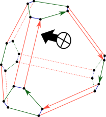
Figure 11.2. The rule for orienting the long and medium edges based on a co-orientation of a large hexagonal face.

It remains to orient the short edges of $\mathcal{T}_{00}$, which is done with the following rule.

Rule 11.9.

We use an outward facing normal vector at each end of an edge of $\mathcal{T}$ and orient the short edges using the right-hand rule (hence, anticlockwise when looking from the boundary).

Although we have chosen an arbitrary ambient orientation of $M$, choosing the opposite orientation results in the reversal of all edges in $\mathcal{T}_{00}$, which does not affect the considerations that follow.

11.3.2. The labelling with $SL(2,\mathbb{C})$ matrices

Suppose that the $1$-cells of the complex $\mathcal{T}_{00}$ are all oriented in the way described above, in terms of the parity $\delta=\delta_{W}$ of a strong combinatorial flattening $W$. We may now label these oriented $1$-cells with the elements of $SL(2,\mathbb{C})$ given below.

Rule 11.10 (Labelling rule).

• Each oriented long edge is labelled by the matrix $\displaystyle S=\begin{bmatrix}0&-1\\ 1&0\end{bmatrix}$.

• Each oriented medium edge is labelled by the matrix $\displaystyle T=\begin{bmatrix}1&-1\\ 0&1\end{bmatrix}$.

• Each oriented short edge is labelled by the matrix

  $$H_{W(\square)}=\begin{bmatrix}\exp\bigl{(}\frac{1}{2}W(\square)\bigr{)}&0\\ 0&\exp\bigl{(}-\frac{1}{2}W(\square)\bigr{)}\end{bmatrix},$$

  where $W(\square)$ is the value of the strong combinatorial flattening $W$ on the quad parallel to the rectangle whose boundary contains the short edge.

Since we wish for this labelling to descend to a projective cocycle under the homomorphism $SL(2,\mathbb{C})\to PSL(2,\mathbb{C})$, it is to be understood that changing the orientation of an edge replaces its label $A\in SL(2,\mathbb{C})$ with $A^{-1}$. Observe in particular that $\displaystyle T^{-1}=\begin{bmatrix}1&+1\\ 0&1\end{bmatrix}$ and $S^{-1}=-S$.

11.4. Cocycle conditions

Our main goal now is to prove that the labelling $\mathcal{L}$ defined by Rule 11.10 has all the desired properties needed to compute obstruction cocycles.

Lemma 11.11.

For every strong combinatorial flattening $W$ for $z$, the labelling $\mathcal{L}$ of Rule 11.10 is a boundary-compatible labelling for $z$ in the sense of Definition 11.2.

Proof.

We split the proof into several steps, verifying one by one the conditions in Definition 11.2.

Step 1: $\mathcal{L}|_{\partial M}$ is an $SL(2,\mathbb{C})$-cocycle.  In order to check condition (i), we must verify the $SL(2,\mathbb{C})$-cocycle conditions for all boundary $2$-cells of $\mathcal{T}_{00}$. We start by considering a boundary hexagon coming from a truncated vertex of a tetrahedron. There are two cases: either all parities $\delta(\square)$, $\delta(\square^{\prime})$, $\delta(\square^{\prime\prime})$ in the tetrahedron are odd or exactly one of them is odd. We shall write $\delta$, $\delta^{\prime}$, $\delta^{\prime\prime}$ for short and consider both cases separately.

Case 1.1: $\delta=\delta^{\prime}=\delta^{\prime\prime}=1$.  Consider a tetrahedron in which the parities are all odd. Hence, the face co-orientations are either all inwards or all outwards. Figure 11.3 shows the case of all co-orientations pointing outwards.

Figure 11.3. A boundary hexagon in a doubly truncated tetrahedron with $\delta=\delta^{\prime}=\delta^{\prime\prime}=1$, viewed from the ideal vertex, with a possible orientation of its edges.

The holonomy around the boundary hexagon is then

$$H_{W^{\prime\prime}}TH_{W^{\prime}}TH_{W}T =\begin{bmatrix}e^{W^{\prime\prime}/2}&-e^{W^{\prime\prime}/2}\\ 0&e^{-W^{\prime\prime}/2}\end{bmatrix}\begin{bmatrix}e^{W^{\prime}/2}&-e^{W^{\prime}/2}\\ 0&e^{-W^{\prime}/2}\end{bmatrix}\begin{bmatrix}e^{W/2}&-e^{W/2}\\ 0&e^{-W/2}\end{bmatrix}$$

$$=\begin{bmatrix}e^{(W+W^{\prime}+W^{\prime\prime})/2}&-b\\ 0&e^{-(W+W^{\prime}+W^{\prime\prime})/2}\end{bmatrix}$$

$$=\begin{bmatrix}1&-b\\ 0&1\end{bmatrix},$$

where

$$b =e^{(W+W^{\prime}+W^{\prime\prime})/2}+e^{(-W+W^{\prime}+W^{\prime\prime})/2}+e^{(-W-W^{\prime}+W^{\prime\prime})/2}$$

$$=1+e^{-W}+e^{W^{\prime\prime}}=1+e^{-Z+i\pi f}+e^{Z^{\prime\prime}-i\pi f^{\prime\prime}}$$

$$=1+(-1)^{\delta}\tfrac{1}{z}+(-1)^{\delta^{\prime\prime}}z^{\prime\prime}=1-\tfrac{1}{z}-\bigl{(}1-\tfrac{1}{z}\bigr{)}=0.$$

When all faces of the tetrahedron are co-oriented inwards, so that the medium edges have orientations opposite to those shown in Figure 11.3, the holonomy around the hexagon is

$$H_{W}^{-1}TH_{W^{\prime}}^{-1}TH_{W^{\prime\prime}}^{-1}T=H_{-W}TH_{-W^{\prime}}TH_{-W^{\prime\prime}}T.$$

Using the previous calculation, we find the above element to be equal to $\left[\begin{smallmatrix}1&-b^{\prime}\\ 0&1\end{smallmatrix}\right]$, where this time

$$b^{\prime} =e^{-(W+W^{\prime}+W^{\prime\prime})/2}+e^{(-W-W^{\prime}+W^{\prime\prime})/2}+e^{(-W+W^{\prime}+W^{\prime\prime})/2}$$

$$=1+e^{W^{\prime\prime}}+e^{-W}=b=0.$$

Therefore, the $SL(2,\mathbb{C})$ cocycle condition holds around the boundary hexagon.

Case 1.2: $\delta=1$, $\delta^{\prime}=\delta^{\prime\prime}=0$.  This is the case of exactly one of the three parity parameters being odd; without loss of generality, we take it to be $\delta$. An example of this situation is shown in Figure 11.4.

Figure 11.4. A possible orientation of edges around a boundary hexagon in a tetrahedron with $\delta=1$ and $\delta^{\prime}=\delta^{\prime\prime}=0$.

In the case presented in the figure, the holonomy around the boundary hexagon equals:

$$H_{W^{\prime\prime}}T^{-1}H_{W^{\prime}}TH_{W}T =\begin{bmatrix}e^{W^{\prime\prime}/2}&e^{W^{\prime\prime}/2}\\ 0&e^{-W^{\prime\prime}/2}\end{bmatrix}\begin{bmatrix}e^{W^{\prime}/2}&-e^{W^{\prime}/2}\\ 0&e^{-W^{\prime}/2}\end{bmatrix}\begin{bmatrix}e^{W/2}&-e^{W/2}\\ 0&e^{-W/2}\end{bmatrix}$$

$$=\begin{bmatrix}e^{(W+W^{\prime}+W^{\prime\prime})/2}&-b\\ 0&e^{-(W+W^{\prime}+W^{\prime\prime})/2}\end{bmatrix}$$

$$=\begin{bmatrix}1&-b\\ 0&1\end{bmatrix},$$

where

$$b =e^{(W+W^{\prime}+W^{\prime\prime})/2}+e^{(-W+W^{\prime}+W^{\prime\prime})/2}-e^{(-W-W^{\prime}+W^{\prime\prime})/2}$$

$$=1+e^{-W}-e^{W^{\prime\prime}}=1+e^{-Z+i\pi f}-e^{Z^{\prime\prime}-i\pi f^{\prime\prime}}$$

$$=1+(-1)^{\delta}\tfrac{1}{z}-(-1)^{\delta^{\prime\prime}}z^{\prime\prime}=1-\tfrac{1}{z}-\bigl{(}1-\tfrac{1}{z}\bigr{)}=0.$$

Likewise, when the directions of all medium arrows are reversed, we obtain the holonomy

$$H_{W^{\prime}}^{-1}T^{-1}H_{W^{\prime\prime}}^{-1}TH_{W}^{-1}T=H_{-W^{\prime}}T^{-1}H_{-W^{\prime\prime}}TH_{-W}T.$$

Using the previous calculation, this matrix product equals $\left[\begin{smallmatrix}1&-b^{\prime}\\ 0&1\end{smallmatrix}\right]$, where

$$b^{\prime} =e^{-(W+W^{\prime}+W^{\prime\prime})/2}+e^{(W-W^{\prime}-W^{\prime\prime})/2}-e^{(W-W^{\prime}+W^{\prime\prime})/2}$$

$$=1+e^{W}-e^{-W^{\prime}}=1+(-1)^{\delta}z-(-1)^{\delta^{\prime}}\tfrac{1}{z^{\prime}}$$

$$=1-z-(1-z)=0.$$

In conclusion, the $SL(2,\mathbb{C})$ cocycle condition around boundary hexagons holds in all cases.

In order to verify the cocycle condition around the edge discs, we consider an edge $E$ of $\mathcal{T}$. Since the orientations of Rule 11.9 are consistent around the boundary of each of the two discs capping off the cylindrical 3-cell around $E$, the holonomy along these boundaries is always

$$\begin{bmatrix}\exp\bigl{(}\frac{1}{2}\sum_{\square}G(E,\square)W(\square)\bigr{)}&0\\ 0&\exp\bigl{(}-\frac{1}{2}\sum_{\square}G(E,\square)W(\square)\bigr{)}\end{bmatrix}=\begin{bmatrix}1&0\\ 0&1\end{bmatrix},$$

where we have used property (ii) of Definition 11.3.

Step 2: Boundary unipotence.  Thanks to Step 1 above, we know that the restriction of the labelling $\mathcal{L}$ to $\partial\mathcal{T}_{00}$ defines a flat $SL(2,\mathbb{C})$-bundle on each component of $\partial M$. We will now show that for each boundary component, the monodromy of this bundle is always unipotent.

Given a closed peripheral curve $\gamma$, we can homotope $\gamma$ into the $1$-skeleton of the cell complex $\partial\mathcal{T}_{00}$, so that $\gamma$ is made up of short and medium edges only. Therefore, the monodromy along $\gamma$ will be a product of elements of the form $H_{W(\square)}^{\pm 1}$ and $T^{\pm 1}$. These matrices are all upper-triangular, so the monodromy along $\gamma$ is also an upper-triangular matrix whose top-left entry is the product of top-left entries of all the matrices being multiplied. Since the top-left entry of $T^{\pm 1}$ is $1$, only the matrices $H_{W(\square)}^{\pm 1}$ contribute to this product. More precisely, the $(1,1)$-entry of the monodromy along $\gamma$ equals

$$\prod_{\square\in Q(\mathcal{T})}\left(e^{W(\square)/2}\right)^{G(\gamma,\square)}=\exp\Bigl{(}\tfrac{1}{2}\sum_{\square\in Q(\mathcal{T})}G(\gamma,\square)W(\square)\Bigr{)}=1.$$

Therefore, both diagonal entries of the monodromy matrix are equal to $1$.

Step 3: $\mathcal{L}$ projects to a $PSL(2,\mathbb{C})$-cocycle.  We must now show that the elements assigned by $\mathcal{L}$ to oriented edges of $\mathcal{T}_{00}$ project to a $PSL(2,\mathbb{C})$-cocycle under the quotient homomorphism $SL(2,\mathbb{C})\to PSL(2,\mathbb{C})$. Step 1 implies that the cocycle condition holds around boundary $2$-cells of $\mathcal{T}_{00}$, so it suffices to study the large hexagonal faces and the rectangles.

As shown in Figure 11.2, the holonomy around the boundary of a large hexagonal face has the form $(TS)^{3}$ and is therefore equal to the identity matrix, as can be verified by direct computation.

It remains to study the holonomy around a rectangle. We denote by $W=W(\square)$ and $\delta=\delta(\square)$ the quantities assigned to the normal quad $\square$ parallel to the rectangle and consider two cases depending on the value of $\delta$.

Case 3.1: $\delta=0$.

Figure 11.5. Holonomy around a rectangular $2$-cell in $\mathcal{T}_{00}$, as viewed from outside the tetrahedron. Shown are two cases depending on the value of the parity parameter $\delta$ on the corresponding normal quadrilateral type. The co-orientations of the adjacent large hexagonal faces, represented by the thick black arrows, induce the orientations of the long edges as in Figure 11.2.

This case is illustrated on the left side of Figure 11.5. The holonomy around the rectangle is

$$H_{W}SH_{W}S^{-1}=-\left(H_{W}S\right)^{2}=\begin{bmatrix}1&0\\ 0&1\end{bmatrix}.$$

In other words, the $SL(2,\mathbb{C})$ cocycle condition is satisfied on a rectangle with $\delta=0$, which in particular implies the $PSL(2,\mathbb{C})$ cocycle condition.

Case 3.2: $\delta=1$.  This case is illustrated on the right side of Figure 11.5. The holonomy around the rectangle is

$$H_{W}SH_{W}S=\left(H_{W}S\right)^{2}=-\begin{bmatrix}1&0\\ 0&1\end{bmatrix}.$$

Therefore, the cocycle condition fails over $SL(2,\mathbb{C})$ when $\delta=1$, even though it still holds after projecting the labelling elements to $PSL(2,\mathbb{C})$. The same situation occurs when both co-orientations point away from the tetrahedron: this is seen by replacing $S$ by $-S$ in the above calculation.

Step 4: Relationship with $\rho$.  Let $\rho$ be the boundary-parabolic $PSL(2,\mathbb{C})$ representation determined, up to conjugacy, by the shape parameter solution $z$ for which $W$ is a strong combinatorial flattening. It remains to justify that the $PSL(2,\mathbb{C})$-cocycle induced from $\mathcal{L}$ recovers the conjugacy class of $\rho$.

A direct construction of a $PSL(2,\mathbb{C})$-cocycle on $\mathcal{T}_{00}$ from the hyperbolic shapes is given in [Si17, §2.3.2]. Therefore, it suffices to show that these two $PSL(2,\mathbb{C})$-cocycles differ by a coboundary.

We denote by $\mathcal{L^{\prime}}$ the cocycle of [Si17], the definition of which we now briefly recall:

• $\mathcal{L^{\prime}}$ labels all long edges in $\mathcal{T}_{00}$ with the complex Möbius transformation $w\mapsto w^{-1}$ represented by the $SL(2,\mathbb{C})$-matrix $R=\left[\begin{smallmatrix}0&i\\ i&0\end{smallmatrix}\right]$.

• Medium edges are labelled with the Möbius transformation $w\mapsto 1-w$, which is the image of $C=\left[\begin{smallmatrix}-i&i\\ 0&i\end{smallmatrix}\right]$ under the quotient homomorphism.

• $\mathcal{L^{\prime}}$ labels each oriented short edge with $\pm H_{Z(\square)}\in PSL(2,\mathbb{C})$.

Note that the Möbius transformations induced by $R$ and $C$ are both involutions, so the choice of orientations of the long and medium edges is not needed in the construction of $\mathcal{L^{\prime}}$. For this reason, $\mathcal{L^{\prime}}$ is defined purely in terms of the shape parameters, without the need for a flattening.

We now explain how to obtain $\mathcal{L}$ from $\mathcal{L^{\prime}}$. Suppose that a strong combinatorial flattening $W$ for $z$ has been chosen and that the $1$-cells of $\mathcal{T}_{00}$ have been oriented accordingly. We shall call a vertex of $\mathcal{T}_{00}$ a sink if it is incident to a medium edge oriented towards it. For each sink vertex, we perform a coboundary action on $\mathcal{L^{\prime}}$, locally conjugating by the Möbius transformation $w\mapsto-w$. Hence, the Möbius transformation labelling the adjacent medium edge becomes

$$\bigl{(}w\mapsto-(1-w)\bigr{)}=\bigl{(}w\mapsto w-1\bigr{)}\sim\pm\begin{bmatrix}1&-1\\ 0&1\end{bmatrix}=\pm T.$$

Similarly, the long edge adjacent to a sink vertex, labelled in $\mathcal{L^{\prime}}$ by the element $w\mapsto w^{-1}$, will conjugate to

$$\bigl{(}w\mapsto(-w)^{-1}\bigr{)}=\bigl{(}w\mapsto\tfrac{-1}{w}\bigr{)}\sim\pm\begin{bmatrix}0&-1\\ 1&0\end{bmatrix}=\pm S.$$

This coboundary modification will also modify the elements $\pm H_{Z(\square)}$ associated to the short edges in $\mathcal{L^{\prime}}$. It is easy to see that this modification amounts to shifting the log-parameters $Z$ by integer multiples of $\pi i$, which has the same effect as replacing them by the values of the flattening $W$. ∎

Corollary 11.12.

As seen in Step 3 of the above proof, the labelling $\mathcal{L}$ satisfies the $SL(2,\mathbb{C})$ cocycle conditions around all $2$-cells of $\mathcal{T}_{00}$ except possibly for the rectangles. Moreover, the holonomy of $\mathcal{L}$ around a rectangle with the parity parameter $\delta=\delta(\square)$ is always $(-1)^{\delta}\left[\begin{smallmatrix}1&0\\ 0&1\end{smallmatrix}\right]$.

Proof of Theorem 11.1.

We begin by showing part (ii). Suppose that $z$ is an algebraic solution of edge consistency and completeness equations on $\mathcal{T}$ and that $W$ is a strong combinatorial flattening for $z$. Denote by $\rho=\rho_{z}$ the associated boundary-parabolic representation $\pi_{1}(M)\to PSL(2,\mathbb{C})$. Using $W$, we construct a boundary-compatible labelling $\mathcal{L}$. By Corollary 11.12, the obstruction class to lifting $\rho$ to a boundary-unipotent $SL(2,\mathbb{C})$-representation is represented by the cocycle $\mathrm{rect}(\delta)\in Z^{2}(\mathcal{T}_{00},\partial\mathcal{T}_{00};\mathbb{F}_{2})$, where $\delta\in\mathbb{F}_{2}^{Q(\mathcal{T})}$ is given in terms of $W$ by equation (11.3). Observe that $\delta(\square)+\delta(\square^{\prime})+\delta(\square^{\prime\prime})=1$ and that $\delta$ has even parity along all unoriented curves in normal position with respect to $\mathcal{T}$. Therefore, $\delta\in\mathcal{A}^{\mathbb{F}_{2}}_{\mathrm{even}}(\mathcal{T})$.

We must now show that $(-1)^{\delta}$ belongs to the same connected component of $\mathcal{S\mkern-2.5muA}_{0}(\mathcal{T})$ as the $S^{1}$-valued angle structure $\omega(\square)=z(\square)/|z(\square)|$. Recall that $\delta(\square)=[f(\square)]_{2}$ where $\pi if(\square)=Z(\square)-W(\square)$. By Definition 11.3, $\operatorname{Im}W\in T\mkern-2.0mu\mathcal{AS}_{0}(\mathcal{T})$, i.e., $\operatorname{Im}Z-\pi f\in T\mkern-2.0mu\mathcal{AS}_{0}(\mathcal{T})$. Since $\exp\bigl{(}i\operatorname{Im}Z(\square)\bigr{)}=\omega(\square)$, Remark 2.4 implies that the circle-valued angle structures $\omega$ and $(-1)^{\delta}$ lie in the same connected component of $\mathcal{S\mkern-2.5muA}_{0}(\mathcal{T})$.

In order to prove part (i), we must consider an algebraic solution $z$ of the edge consistency equations which does not necessarily satisfy the completeness equations. Let $\rho$ be the associated $PSL(2,\mathbb{C})$ representation and let $\omega(\square)=z(\square)/|z(\square)|$ be the $S^{1}$-valued angle structure determined by $z$. Once again, we may choose log-parameters $Z(\square)$ such that $Z(\square)+Z(\square^{\prime})+Z(\square^{\prime\prime})=i\pi$ in every tetrahedron. Let $c\in 2\mathbb{Z}^{\mathcal{E}(\mathcal{T})}$ be the even vector given by $\mathbf{G}Z=\pi ic$. By Theorem 3.12, there exists a vector $\eta\in\mathbb{Z}^{Q(\mathcal{T})}$ such that $\eta(\square)+\eta(\square^{\prime})+\eta(\square^{\prime\prime})=1$ in every tetrahedron, $\mathbf{G}\eta=c$, and moreover $\eta$ has even parity along all curves in normal position with respect to $\mathcal{T}$. Therefore, $W(\square):=Z(\square)-i\pi\eta(\square)$ satisfies all of the conditions in the definition of a strong combinatorial flattening except for the vanishing of $\mathbf{G_{\partial}}W$.

Using Rule 11.10, we may produce a labelling $\mathcal{L}$ of $1$-cells of $\mathcal{T}_{00}$ with elements of $SL(2,\mathbb{C})$ in terms of $W$. Since the representation $\rho$ is not assumed boundary-parabolic, the labelling $\mathcal{L}$ will not induce boundary-unipotent representations of the peripheral subgroups. Nonetheless, Steps 1, 3 and 4 in the proof of Lemma 11.11 do not require this assumption and therefore can be repeated without modification. In particular, for $\delta=[\eta]_{2}$ we have $\delta\in\mathcal{A}^{\mathbb{F}_{2}}_{\mathrm{even}}(\mathcal{T})$ and $[\mathrm{rect}(\delta)]=\operatorname{Obs}(\rho)\in H^{2}(M;\mathbb{F}_{2})$. Moreover, $(-1)^{\delta}$ lies in the same connected component of $\mathcal{S\mkern-2.5muA}(\mathcal{T})$ as $\omega$, because $\operatorname{Im}W\in T\mkern-2.0mu\mathcal{AS}(\mathcal{T})$. ∎

Appendix A The asymptotic expansion of the $q$-dilogarithm

In this appendix we will explain how to obtain the asymptotic expansion given in equation (5.3) using the method of Mellin transforms. See [FGD95] for a clear exposition of this method.

We fix arbitrarily the parameter $\omega\in\mathbb{C}$ satisfying $|\omega|=1$ and $\omega\neq 1$, as well as the parameter $a\in\mathbb{C}$ with $\operatorname{Re}a>0$. In terms of the negative real parameter $\hbar<0$, the expansion is

$$\mathrm{Li}_{2}(\omega e^{a\hbar};e^{\hbar})=-\mathrm{Li}_{2}(\omega)\hbar^{-1}+(a-{\textstyle\frac{1}{2}})\log(1-\omega)-\sum_{k=1}^{\infty}\frac{B_{k+1}(a)}{(k+1)!}\mathrm{Li}_{1-k}(\omega)\,\hbar^{k}$$

as $\hbar\to 0^{-}$. The analogous formula for the case $\omega=1$, equation (5.2), was obtained by Zhang using a short and conceptually attractive Mellin transform argument. The formula is stated as Theorem 2 in [Zh14] and is clearly explained there. This approach will be convenient for generalisation to the case $\omega\neq 1$.

To match the discussion in [Zh14] we set $\hbar=-x$, for $x>0$, and consider $\mathrm{Li}_{2}(\omega e^{-ax};e^{-x})$ as $x\rightarrow 0^{+}$. The heart of the computation of the case $\omega=1$ is equation (3.1) of [Zh14] which presents the computation of the Mellin transform of the function $\mathrm{Li}_{2}(e^{-ax};e^{-x})$,

$$\int_{0}^{\infty}\mathrm{Li}_{2}(e^{-ax};e^{-x})x^{s-1}\;dx=\Gamma(s)\zeta(s+1)\zeta(s,a).$$

Here

• $\Gamma(s)$ is the Euler gamma function,

• $\zeta(s)$ is the Riemann zeta function $\zeta(s)=\sum_{n=1}^{\infty}\frac{1}{n^{s}}$,

• and $\zeta(s,a)=\sum_{n=0}^{\infty}\frac{1}{(a+n)^{s}}$ is the Hurwitz zeta function.

The calculation leading to this formula is Section 4.2 of [Zh14]. When the phase term $\omega$ is introduced into this calculation, it is straightforward to compute that the only difference in the result is that the Riemann zeta function factor $\zeta(s+1)$ is generalised to the Lerch zeta function:

$$\zeta_{\omega}(s+1)=\sum_{n=1}^{\infty}\frac{\omega^{n}}{n^{s+1}}.$$

In other words:

(A.1) $$\int_{0}^{\infty}\mathrm{Li}_{2}(e^{-ax}\omega;e^{-x})x^{s-1}\;dx=\Gamma(s)\zeta_{\omega}(s+1)\zeta(s,a).$$

To be able to apply the inverse Mellin transform along some vertical contour in the $s$-plane, $\gamma:\mathbb{R}\rightarrow\mathbb{C}$, $\gamma(t)=c+it$, for some fixed $c>1$, it is sufficient to know that the Mellin transform (A.1) is integrable along that contour (see Theorem 2 of [FGD95]). Zhang checks this for the $\omega=1$ case $\Gamma(s)\zeta(s+1)\zeta(s,a)$ using the asymptotics of $\Gamma(c+it)$ and $\zeta(c+it,a)$ as $t\rightarrow\pm\infty$ (see Lemma 5 of [Zh14]). When $\zeta(s)$ is replaced by $\zeta_{\omega}(s)$ one can see that there is no change needed to this argument because

$$|\zeta_{\omega}(c+it)|\leq\zeta(c)$$

and hence the Lerch zeta factor is bounded on the contour. Thus the asymtptotics given in [Zh14] for $\Gamma(c+it)$ and $\zeta(c+it,a)$ still imply integrability in the case $\omega\neq 1$. As a consequence,

(A.2) $$\mathrm{Li}_{2}(e^{-ax}\omega;e^{-x})=\frac{1}{2\pi i}\int_{c-i\infty}^{c+i\infty}\Gamma(s)\zeta_{\omega}(s+1)\zeta(s,a)\frac{1}{x^{s}}\;ds.$$

Following the method of Mellin transforms [FGD95], we will now apply residue calculus to convert the integral (A.2) into an asymptotic expansion. Note that the integral is of the order $O(x^{-c})$ and that the integrand can be continued meromorphically onto the whole $s$-plane.

The method is to shift the horizontal position of the vertical contour to the left. When the contour crosses a pole, the expression picks up a term from the residue at that pole. So if $d<c$, and $P$ denotes the set of poles of $\Gamma(s)\zeta_{\omega}(s+1)\zeta(s,a)\frac{1}{x^{s}}$ lying between the vertical contours at $d$ and $c$, then

(A.3) $$\mathrm{Li}_{2}(e^{-ax}\omega;e^{-x})=\sum_{p\in P}\operatorname*{Res}_{s=p}\left(\Gamma(s)\zeta_{\omega}(s+1)\zeta(s,a)\frac{1}{x^{s}}\right)+O(x^{-d}).$$

It remains for us to understand the poles of $\Gamma(s)\zeta_{\omega}(s+1)\zeta(s,a)\frac{1}{x^{s}}$ and the residues at those poles under the assumption that $\omega\neq 1$:

• When $\omega\neq 1$, the Lerch zeta function $\zeta_{\omega}(s+1)$ is entire and has no poles [Ap51].

• The Hurwitz zeta function $\zeta(s,a)$ has a simple pole at $s=1$ with the corresponding residue equal to $1$ [Zh14].

• The gamma function $\Gamma(s)$ has simple poles at all non-positive integers $s=-k$ with corresponding residues $\frac{(-1)^{k}}{k!}$. (See [Er53, Zh14].)

In summary, the Mellin transform (A.1) has simple poles at $s\in\{1,0\}\cup\{-k,\;k\in\mathbb{N}\}$.

To determine the corresponding residues, we will need the following formula for the values of the Lerch zeta function at the non-positive integers $m\leq 0$:

(A.4) $$\zeta_{\omega}(m)=\mathrm{Li}_{m}(\omega).$$

This formula can be obtained from the analysis in Apostol [Ap51]. To relate our notations to the formulae in [Ap51], note that for a real $t$ such that $\omega=\exp(2\pi it)$ and a complex $s$, we have

$$\zeta_{\omega}(s)=\zeta_{\exp(2\pi it)}(s)=e^{2\pi it}\phi(t,1,s),$$

where $\phi$ is the function defined in equation (1.1) of [Ap51], also known as the Lerch transcendent. Then the case $m=0$ of equation (A.4) is given at the start of Section 3 in [Ap51]:

$$\zeta_{\exp(2\pi it)}(0)=e^{2\pi it}\phi(t,1,s)=e^{2\pi it}\frac{1}{1-e^{2\pi it}}=\mathrm{Li}_{0}(\omega),$$

using equation (5.1). Furthermore, the differential equation

$$\frac{\partial}{\partial t}\phi(t,a,s)+2\pi ia\phi(t,a,s)=2\pi i\phi(t,a,s-1),$$

given in [Ap51, eq. (2.6)], can be used to derive a recursion relation as follows:

$$\zeta_{\omega}(s-1) =e^{2\pi it}\phi(t,1,s-1)$$

$$=\frac{1}{2\pi i}\left(e^{2\pi it}\frac{\partial}{\partial t}\phi(t,1,s)+2\pi ie^{2\pi it}\phi(t,1,s)\right)$$

$$=\frac{1}{2\pi i}\frac{\partial}{\partial t}\left(e^{2\pi it}\phi(t,1,s)\right)$$

$$=\frac{1}{2\pi i}\frac{\partial}{\partial t}\zeta_{\exp(2\pi it)}(s)$$

$$=\frac{1}{2\pi i}\left(\frac{\partial}{\partial t}e^{2\pi it}\right)\frac{\partial}{\partial\omega}\zeta_{\omega}(s)=\omega\frac{\partial}{\partial\omega}\zeta_{\omega}(s).$$

Thus the two sides of (A.4) coincide at $m=0$ and satisfy the same recursion relation, so the equation is established for all $m\leq 0$.

Now we can turn to computing the residues of $\Gamma(s)\zeta_{\omega}(s+1)\zeta(s,a)\frac{1}{x^{s}}$:

• The residue at the pole at $s=1$ equals:

  $$\Gamma(1)\zeta_{\omega}(1+1)\operatorname*{Res}_{s=1}\bigl{(}\zeta(s,a)\bigr{)}\frac{1}{x^{1}}=1\cdot\left(\sum_{n=1}^{\infty}\frac{\omega^{n}}{n^{2}}\right)\cdot 1\cdot\frac{1}{x}=\mathrm{Li}_{2}(\omega)\frac{1}{x}.$$

• The residue at the pole at $s=0$ equals:

  $$\operatorname*{Res}_{s=0}\bigl{(}\Gamma(s)\bigr{)}\zeta_{\omega}(1)\zeta(0,a)\frac{1}{x^{0}}=1\cdot\left(\sum_{n=1}^{\infty}\frac{\omega^{n}}{n}\right)\cdot\bigl{(}\tfrac{1}{2}-a\bigr{)}=\left(a-\tfrac{1}{2}\right)\ln(1-\omega)$$

  using the evaluation $\zeta(0,a)=\frac{1}{2}-a$; cf. [Er53, eq. 1.10(8)].

• The residue at the pole at $s=-k$, where $k\in\mathbb{N}$, equals:

  $$\operatorname*{Res}_{s=-k}\bigl{(}\Gamma(s)\bigr{)}\zeta_{\omega}(1-k)\zeta(-k,a)x^{k}=\frac{(-1)^{k}}{k!}\cdot\zeta_{\omega}(1-k)\cdot\left(-\frac{B_{k+1}(a)}{k+1}\right)x^{k}.$$

  By virtue of equation (A.4), this equals

  $$-\frac{1}{(k+1)!}B_{k+1}(a)\mathrm{Li}_{1-k}(\omega)(-x)^{k}.$$

Substituting these calculations in equation (A.3) and putting $\hbar=-x$ yields the asymptotic expansion given in equation (5.3).

References

- [AK12] Jørgen Ellegaard Andersen and Rinat Kashaev. A TQFT from quantum Teichmüller theory. arXiv preprint arXiv:1109.6295v2, 2012.
- [AK13] Jørgen Ellegaard Andersen and Rinat Kashaev. A new formulation of the Teichmüller TQFT. arXiv preprint arXiv:1305.4291, 2013.
- [Ap51] Tom M. Apostol. On the Lerch zeta function. Pacific Journal of Mathematics, 1(2):161–167, 1951.
- [Ba10] Ernest W. Barnes. A transformation of the generalised hypergeometric series. Quarterly Journal of Pure and Applied Mathematics, 41:136–140, 1910.
- [BH16] Fethi Bouzeffour and Borhen Halouani. On the asymptotic expansion of the -dilogarithm. Advances in Difference Equations, 2016(1):1–9, 2016.
- [CY18] Qingtao Chen and Tian Yang. Volume conjectures for the Reshetikhin–Turaev and the Turaev–Viro invariants. Quantum Topology, 9(3):419–460, 2018.
- [Ch04] Young-Eun Choi. Positively oriented ideal triangulations on hyperbolic three-manifolds. Topology, 43(6):1345–1371, 2004.
- [Cl32] Thomas Clausen. Über die Function . Journal für die reine und angewandte Mathematik, 8(III):298–300, 1832.
- [Cu86] Marc Culler. Lifting representations to covering groups. Advances in Mathematics 59(1):64–70, 1986.
- [Di13] Tudor Dimofte. Quantum Riemann surfaces in Chern-Simons theory. Advances in Theoretical and Mathematical Physics 17(3):479–599, 2013.
- [DGG13] Tudor Dimofte, Davide Gaiotto, and Sergei Gukov. 3-manifolds and 3D indices. Advances in Theoretical and Mathematical Physics, 17(5):975–1076, 2013.
- [DGG14] Tudor Dimofte, Davide Gaiotto, and Sergei Gukov. Gauge theories labelled by 3-manifolds. Communications in Mathematical Physics, 325(2):367–419, 2014.
- [DG13] Tudor Dimofte and Stavros Garoufalidis. The quantum content of the gluing equations. Geometry & Topology, 17(3):1253–1315, 2013.
- [Er53] Arthur Erdélyi et al. Higher transcendental functions, Vol. I. McGraw-Hill, 1953.
- [FGD95] Philippe Flajolet, Xavier Gourdon, and Philippe Dumas. Mellin transforms and asymptotics: harmonic sums. Theoretical Computer Science, 144(1–2):3–58, 1995.
- [Fr04] Stefano Francaviglia. Hyperbolic volume of representations of fundamental groups of cusped 3-manifolds. International Mathematics Research Notices, 9:425–459, 2004.
- [FG11] David Futer and François Guéritaud. From angled triangulations to hyperbolic structures. Interactions Between Hyperbolic Geometry, Quantum Topology and Number Theory. Contemporary Mathematics, 541:159–182, 2011.
- [Ga16] Stavros Garoufalidis. The 3D index of an ideal triangulation and angle structures. Ramanujan Journal, 40(3):573–604, 2016.
- [GHHR16] Stavros Garoufalidis, Craig D. Hodgson, Neil R. Hoffman and J. Hyam Rubinstein. The 3D-index and normal surfaces. Illinois Journal of Mathematics, 60(1):289–352, 2016.
- [GHRS15] Stavros Garoufalidis, Craig D. Hodgson, J. Hyam Rubinstein, and Henry Segerman. 1-eficient triangulations and the index of a cusped hyperbolic 3-manifold. Geometry and Topology, 19(5):2619-2689, 2015.
- [GK19] Stavros Garoufalidis and Rinat Kashaev. A meromorphic extension of the 3D-index. Research in the Mathematical Sciences, 6:8, 2019.
- [GM93] Francisco González-Acuña and José María Montesinos-Amilibia. On the character variety of group representations in and . Mathematische Zeitschrift, 214(1):627–652, 1993.
- [GTZ15] Stavros Garoufalidis, Dylan P. Thurston and Christian K. Zickert. The complex volume of -representations of -manifolds. Duke Mathematical Journal, 164(11):2099–2160, 2015.
- [HP04] Michael Heusener and Joan Porti. The variety of characters in . Boletín de la Sociedad Matemática Mexicana, series, special issue in vol. 10, pp. 221–237, 2004.
- [HRS12] Craig D. Hodgson, J. Hyam Rubinstein, and Henry Segerman. Triangulations of hyperbolic -manifolds admitting strict angle structures. Journal of Topology, 5(4):887–908, 2012.
- [Ka95] Rinat M. Kashaev. A link invariant from quantum dilogarithm. Modern Physics Letters A, 10(19):1409–1418, 1995.
- [Ka97] Rinat M. Kashaev. The hyperbolic volume of knots from the quantum dilogarithm. Letters in Mathematical Physics, 39(3):269–275, 1997.
- [Ka14] Rinat M. Kashaev. Beta pentagon relations. Theoretical and Mathematical Physics, 181(1):1194–1205, 2014.
- [Kas] Rinat M. Kashaev. private communication.
- [KLV16] Rinat M. Kashaev, Feng Luo, and Grigory Vartanov. A TQFT of Turaev–Viro type on shaped triangulations. Annales Henri Poincaré, 17:1109–1143, 2016.
- [Ki95] Anatol N. Kirillov. Dilogarithm identities. Progress of theoretical physics supplement, 118:61–142, 1995.
- [La00] Mark Lackenby. Taut ideal triangulations of –manifolds. Geometry & Topology, 4(1):369–95, 2000.
- [Lu13] Feng Luo. Volume optimization, normal surfaces, and Thurston’s equation on triangulated -manifolds. Journal of Differential Geometry, 93(2):299–326, 2013.
- [Lu16] Feng Luo. Solving Thurston’s equation in a commutative ring. Journal of Topology, 9:143–160, 2016.
- [m3di] Rafał Siejakowski. m3di: a program for computing the meromorphic 3D-index. Available at https://github.com/S-Rafael/m3di, 2021.
- [MI99] Richard J. McIntosh. Some asymptotic formulae for -shifted factorials. The Ramanujan Journal, 3(2):205–214, 1999.
- [MM01] Hitoshi Murakami and Jun Murakami. The colored Jones polynomials and the simplicial volume of a knot. Acta Mathematica, 186(1):85–104, 2001.
- [Ne92] Walter Neumann. Combinatorics of triangulations and the Chern–Simons invariant for hyperbolic -manifolds. Topology ‘90, pp. 243-272, 1992.
- [Ne04] Walter Neumann. Extended Bloch group and the Cheeger–Chern–Simons class. Geometry & Topology, 8(1):413–474, 2004.
- [NZ85] Walter Neumann and Don Zagier. Volumes of hyperbolic three-manifolds. Topology, 24(3):307–332, 1985.
- [PK01] Richard B. Paris and David Kaminski. Asymptotics and Mellin–Barnes Integrals. Cambridge University Press, 2001.
- [Po97] Joan Porti. Torsion de Reidemeister pour les variétés hyperboliques. Memoirs of the AMS, 128(612), 1997.
- [Pto] Matthias Görner. The ‘ptolemy’ module: Data for the SnapPy manifolds. Browsable online database published at http://ptolemy.unhyperbolic.org.
- [Reg] B. Burton, R. Budney, W. Pettersson et al. Regina: Software for low-dimensional topology. Available at https://regina-normal.github.io/, 1999–2020.
- [RST] J. Hyam Rubinstein, Henry Segerman, Stephan Tillmann. Traversing three-manifold triangulations and spines. Enseign. Math., 65(1-2):155–206, 2019.
- [Si17] Rafał Siejakowski. On the geometric meaning of the non-abelian Reidemeister torsion of cusped hyperbolic 3-manifolds. PhD thesis, Nanyang Technological University Singapore, 2017.
- [Si21] Rafał Siejakowski. Infinitesimal gluing equations and the adjoint hyperbolic Reidemeister torsion. Tohoku Mathematical Journal, 73(4), 2021.
- [Sl66] Lucy Joan Slater. Generalized hypergeometric functions. Cambridge University Press, 1966.
- [Sn] Marc Culler, Nathan M. Dunfield, Matthias Goerner, and Jeffrey R. Weeks. SnapPy, a computer program for studying the geometry and topology of -manifolds. Available at http://snappy.math.uic.edu.
- [Th80] William Thurston. The geometry and topology of three-manifolds. 1980; electronic version dated 2002 retrieved from http://library.msri.org/books/gt3m/.
- [To98] Jeffrey L. Tollefson. Normal surface Q-theory. Pacific Journal of Mathematics, 183(2):359–374, 1998.
- [Yo91] Tomoyoshi Yoshida. On ideal points of deformation curves of hyperbolic 3-manifolds with one cusp. Topology, 30(2):155–170, 1991.
- [Za07] Don Zagier. The dilogarithm function. In Frontiers in number theory, physics, and geometry II, pp. 3–65. Springer Verlag, 2007.
- [Zh14] Ruiming Zhang. On asymptotics of the -exponential and -gamma functions. Journal of Mathematical Analysis and Applications, 411:522–529, 2014.
- [Zi09] Christian K. Zickert. The volume and Chern–Simons invariant of a representation. Duke Mathematical Journal, 150(3):489-532, 2009.