Border-SegGCN: Improving Semantic Segmentation by Refining the Border Outline using Graph Convolutional Network

Abstract

We present Border-SegGCN, a novel architecture to improve semantic segmentation by refining the border outline using graph convolutional networks (GCN). The semantic segmentation network such as Unet or DeepLabV3+ is used as a base network to have pre-segmented output. This output is converted into a graphical structure and fed into the GCN to improve the border pixel prediction of the pre-segmented output. We explored and studied the factors such as border thickness, number of edges for a node, and the number of features to be fed into the GCN by performing experiments. We demonstrate the effectiveness of the Border-SegGCN on the CamVid and Carla dataset, achieving a test set performance of 81.96% without any post-processing on CamVid dataset. It is higher than the reported state of the art mIoU achieved on CamVid dataset by 0.404%.

1 Introduction

Semantic segmentation provides dense per pixel classification corresponding to each pixel’s labels [3, 10, 16], which is a crucial task in the field of computer vision. Solving and understanding the environment within an image using segmentation opens the door to many applications in the field of robotics, security, autonomous vehicles, helping blind and visually impaired people (BVIP), etc. With the advancements in deep neural networks, [12, 43, 27, 45], computer vision tasks such as semantic segmentation performance have improved using large scale datasets for training as compared to segmentation using handcrafted features [21, 28, 57, 20]. Segmentation of pixels in non-boundaries regions is easier than for the object boundaries, since border pixels are prone to have large ambiguity in belonging to a particular segment.

Graph convolutional network Research in the field of Graph Neural Networks (GNN) have produced interesting results for graph classification that do not require as much resources as traditional Neural networks [26]. Graph Convolutional Networks (GCN) have been used in the field of body pose estimation, action recognition, etc, as human body data can be converted into graphical forms [50, 62, 61, 56, 30, 19, 36]. Similarly, point cloud data has also been used in graphical forms. [42, 54, 29].

As illustrated in Figure 1, we propose a novel GCN based architecture for refining the outline of object boundaries on the pre-segmented image from a baseline network such as Unet or any other arbitrary network. Instead of focusing on the whole video segmentation task using GCNs, we focus on improving the object boundaries causing more ambiguities at the boundaries than at the non-border regions. The loss function penalizes for the border pixels in the network. It also decreases the computation complexity for the whole network as it has to only focus on some regions of the whole scene in each frame of a video. We effectively build a pipeline to generate graph based data from the visual data using spatial and intensity information of the pixels. Our architecture gives the flexibility to use any baseline network for the pre-segmentation task. We performed evaluation using two baseline networks to study the effect of using very different baseline network. In addition, a visualization analysis reveals that the object outline segmentation learned by the proposed architecture has meaningful semantic predictions.

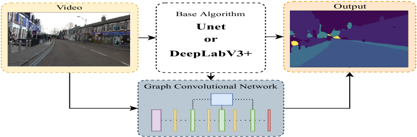
Figure 1: We aim to adapt a semantic segmentation model learned from base algorithm using a graph convolutional network (GCN). The initial segmentation from base algorithm is used as basis and thereafter, GCNs are used to improve the object border outline pixel classification.

Our contributions are summarized as follows: (1) We develop a novel method, Border-SegGCN, using GCNs to improve the semantic segmentation performance by refining the predicted boundaries. (2) We test our pipeline using two open source datasets, i.e., Camvid and Carla dataset (3) We perform the evaluation of different border widths to be used for a better performance of the procedure. (4) We evaluate the performance with a varying number of edges for the nodes in the graph. (5) We study the effect of a different number of features used as an input to the GCN network. (6) We evaluate the training with different hyper-parameters such as dropout and regularisation. (7) We also verify the performance of Border-SegGCN visually using qualitative results. (8) We prove the performance of the network using two different baseline models, i.e., Unet and DeepLabV3+. Border-SegGCN consistently improves performance when used on top of baseline approaches.

2 Related Work

Semantic segmentation is actively researched by computer vision researchers due to its application in various domains such as robotics, health care, security, etc. Most recent work is using fully convolutional neural networks for pixel-wise classification [43, 39, 60, 32, 33]. Various model variants have been researched [8, 46, 23, 49] to use the contextual information for the task of segmentation [38, 11, 57, 28] based on multi-scale inputs [18, 15, 34] or based on probabilistic graphical models [40, 5, 6, 7]. There are many open-source datasets available for semantic segmentation, such as e.g., PASCAL [17], COCO [35], CamVid [4], Carla [13], etc. Our work uses the CamVid and Carla dataset for the semantic segmentation task. We use Unet and DeepLabV3+ as our base networks for the segmentation.

Graph neural networks have recently been used for various applications involving the graph structured data because of their effectiveness in representing such data [52]. Some of the tasks are action recognition, body pose estimation, link prediction, etc. Graph models can be subdivided into two categories, i.e, Graph Neural Network (GNN) [53, 51, 41, 37, 59, 31, 24], and GCNs.

The first category, i.e., GNN, consists of a graph and a recurrent neural network and has a functionality of passing messages and updating nodes states which store the semantic and structural information in the neighboring nodes. For instance, [41] uses a 3D graph neural network (3DGNN) with a 3D point cloud to build a k-nearest neighbor graph for RGBD semantic segmentation. Every node in the graph represents a group of points which has a hidden representation vector that is updated based on the recurrent functions.

The second category, i.e., GCN, extends the mathematical operation of convolution to graph structures. GCNs can be distinguished into two types, i.e., spectral GCNs and spatial GCNs. Spectral GCNs convert signals in graphical form into graph spectral domains, in which they can be manipulated using spectral filters. For instance, in [14, 22], graph Laplacian-based CNNs are used in the spectral domain. Spectral GCNs use convolution along with neighborhood data to calculate the feature vector for the node. They were first employed for semi-supervised classification on graph-structured data [26]. For example, [48] use GCNs on point cloud data in the spatial domain. [47] use GCNs in a recurrent structure for skeleton based action recognition.

Both [1] and [58] have shown that image semantic segmentation can be formulated and solved using graphs. This paper focuses on applying GCNs in the context of video segmentation. The main issues discussed revolve around creating an efficient pipeline to convert video frames into graphs and optimising the pipeline to maximizing the efficiency of the GCN.

3 Methodology

Figure 1 illustrates an overview of the used pipeline. In the following section, we will discuss how we approach the graph creation from an image.

3.1 Efficient Graph Generation

This approach includes a refinement of borders using existing segmentation algorithms. We use the Unet [44] and DeepLabv3+ architecture as a base segmentation networks. The dataset used for the evaluation of this architecture is the Cambridge-driving Labeled Video Database (”CamVid”) dataset [2] and Carla dataset [13]. The frame size is 360 pixels wide and 480 pixels high. A mask is used to determine which nodes to compute based on their location, while omitting the rest of the nodes. This allows the graph to have the same size from frame to frame. Performing computation on the selected nodes allows decreasing computation time drastically and provides more relevant training examples to the GCN.

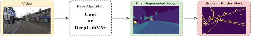
Figure 2: Example of how the data is processed during the Boolean mask generation. Left: The initial frame is passed on to the base segmentation algorithm. Center: An initial rough segmentation is retrieved. Right: Pixels are either selected (yellow) or rejected (purple) depending if they are on the border of different objects.

To determine which nodes are selected we use the initial segmentation that our base algorithm provides: in this case the Unet or DeepLabV3+. With the pre-segmentation provided, boundaries around the objects and different classes are determined. Depending on the task at hand, the pixels that lay on the border are then selected for further processing followed by training or prediction. Figure 2 shows the process of generating the Boolean mask.

3.2 Generating the Features

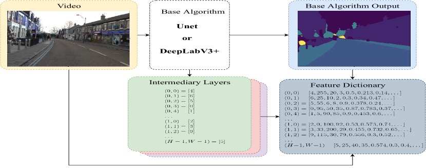
Figure 3: Pipeline for feature extraction from the initial frame. Each feature set is concatenated into a single feature dictionary with the pixel coordinates being the keys of the hash map. Each pixel has at least the class predicted by the base algorithm and the associated RGB values. Intermediate layer values are very dependant on the base algorithm.

Features used for each node consist of the intensity values from the three RGB channels of the video and the output segmented image from the base algorithm such as from Unet or DeepLabV3+. All other features consist of the intermediate values. In case of Unet, the final layers provide features and for the DeepLabV3+, the intermediate layers are used as features for input to GCN. Figure 3 illustrates the pipeline for feature extraction.

3.3 Connecting the Graph

Based on the Boolean mask, nodes are connected that are on the border of objects. The rest of the nodes are either isolated or have only incoming connections.

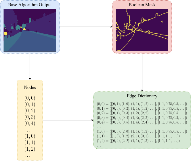
Figure 4: Pipeline for generating the edges of the graph. The first segmented image provides the size of the image and thus all the potential nodes that need to be processed. The Boolean mask directs which nodes should actually be worked on. If a pixel does not reside on a border then it will remain an isolated node.

For each node, the mapping consists of two parts: The actual coordinates of the N closest neighbours denoted by $(x_{i},y_{i})$ with $i<N$, and the weights that are associated with each of those neighbours denoted by $d_{i}$ with $i<N$. The illustration of the pipeline for generating the edges is shown in Figure 4.

The weights associated for the edge between two neighbours are completely arbitrary. We chose to use a weight definition that takes into account the distance and intensity differences as inspired by [1]. The resulting weight definition is shown in Equation 1.

$$\centering d_{n_{12}}=\frac{1}{d_{E_{12}}}\times\exp({-\frac{\left\lVert I_{n_{1}}-I_{n_{2}}\right\rVert}{\left\lVert I_{255}\right\rVert}})\@add@centering$$ (1)

Equation 1 represents the weight between two nodes $n_{1}$ and $n_{2}$ in the $[0,1]$ range. The inverse of the Euclidean distance between these two nodes denoted as $d_{E_{12}}$. The difference in intensities of the two pixels is taken into account for determining the weight of the edge. This value is normalized and its exponent is taken to penalise two nodes of different values. Considering that several operations have to be performed on each neighbour of every selected node, the overall computational cost is $O(n^{k})$ with $n$ being the number of pixels selected, and $k$ the number of closest neighbours we would like to connect to. The Boolean mask assists in directing the resources. If a node is not marked as being on the border, the number of neighbours collapses to 0 in our dictionary. Thus, no computation is performed.

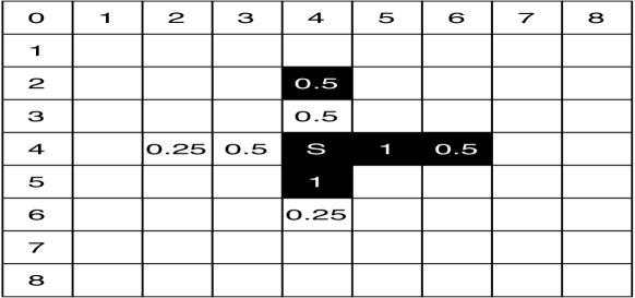
Figure 5: Weights taking into account Euclidean distance and difference in pixel-intensity values.

Figure 5 illustrates the behaviour of Equation 1. The selected node is denoted as S on the grid. The values in each square represent the value of the weight between S and the node that contains the value. If the colours match and the node is directly adjacent, then the value is maximal. On the other hand, two pixels can be next to each other but with different shades of the same colour. In this case, the value will decrease. We thus encode both the spatial information and also the pixel intensity similarity.

3.4 Encoding the Graph

The input to GCN requires the generation of the associated adjacency and feature matrices. The resulting size of these two matrices depend on the initial size of the frame and on the feature set that was selected. An example is the CamVid dataset which provides frames of 360 by 480 pixels in a video. This creates a square adjacency matrix of 172’800 by 172’800 pixels for each frame. The feature matrix will depend on the selected features and in the case where only intensity values of 3 RGB channels of frames are used as features, the shape will be equal to 172’800 $\times$ 3.

4 GCN Training

After the data has been correctly generated as explained in the previous sections (3.1-3.4), the training is carried out. The employed GCN architecture in our Border-SegSGN is a modification on the network given in [26]. The architecture used consists of consecutive graph convolutional layers and dropout layers as shown in Figure 6. We experimented with several different versions of network architecture but the Figure 6 has better performance.

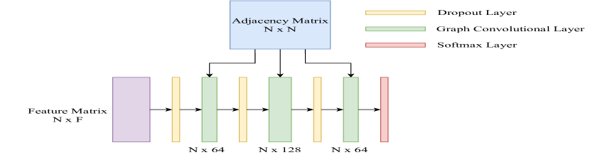
Figure 6: Illustration of our GCN architecture based on [26].

The graph convolutional layers take two input matrices: the adjacency matrix and the feature matrix. The adjacency matrix is considered immutable and thus does not change between the layers. On the other hand, the feature matrix varies with each layer.

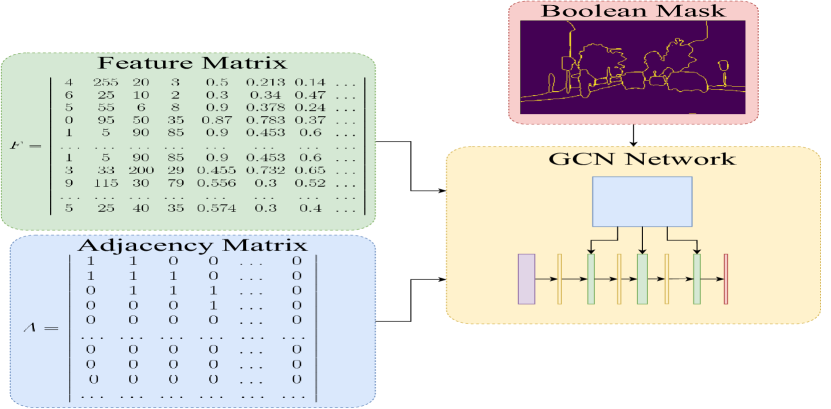
Figure 7: Pipeline representing the inputs for the GCN training in Border-SegGCN.

However, most importantly, we use the Boolean mask created before to direct the GCN training. For the model to fit the correct labels, we pass the mask giving no training relevance on the loss function for the nodes that are not on the border. Figure 7 shows the different inputs to the GCN Network.

5 GCN Prediction

For the prediction as shown in Figure 8, the GCN takes as input the desired adjacency matrix and feature matrix, but does not require the Boolean mask. We predict the class of every node. Due to the nature of the training, the GCN output is poor on pixels that do not lie on any borders. The solution is to combine the base output of the initial algorithm with the output of the GCN where non-border pixels are assigned to their classes from the output of the base algorithm, while border pixels are assigned to their classes from the GCN output.

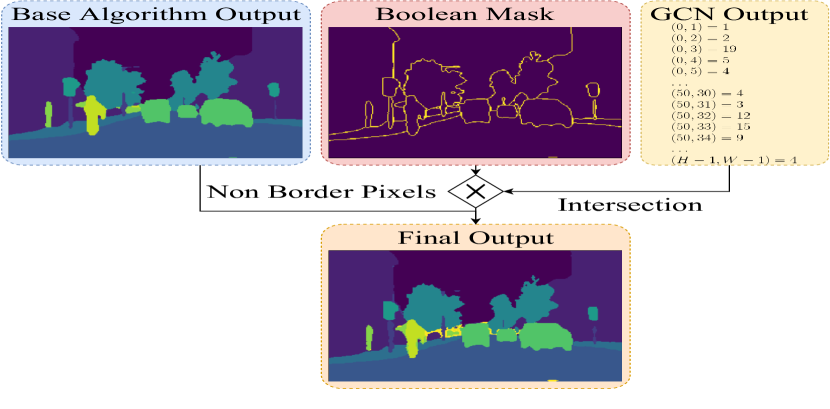
Figure 8: Pipeline of required inputs to generate final segmented image in Border-SegGCN.

6 Experiments

In this section, we verify the effectiveness of our proposed approach for semantic segmentation.

6.1 Implementation Details

We use the Unet implementation of the ”Segmentation models” PyTorch library [55]. The encoder is ResNeXt-50 (32$\times$4d) and the weights of the network are pre-trained from ImageNet. For DeepLabV3+, we use the openly available pre-trained model from [63] based on[9]. For both models, we register forward hooks after each layer and retrieve data at each step for every passing frame. The GCN architecture is modelled based on [26] with slight modifications. It consists of three graph convolutional layers with 64, 128 and 64 channels respectively. A dropout layer is inserted between each graph convolutional layer. The GCN is built in Keras using the ”Spektral” library and an Adam [25] optimiser with a learning rate of 0.001. This approach assumes that each pixel is a sample and this is why it is necessary to set a batch size of $N=H\times W$, where $H$ is the height of frame and $W$ is its width. As a metric for evaluation, we use the mean intersection over union (mIoU) score as defined in [63].

6.2 Dataset

Camvid We use the ”CamVid” [2] dataset for the evaluation of Border-SegGCN. It consists of 367 training, 233 testing, and 101 validation fully annotated frames. Each frame is $360\times 480$ pixels. The testing frames are from two different video sequences, Seq05VD and 0001TP. We do not perform any kind of augmentation on the data for training. We work with the 11 recommended classes out of the 31 available ones to be able to compare with other literature that have followed similar approaches of using 11 classes [63].

Carla [13] is a semantic segmentation dataset for self-driving cars. t is a simulated dataset and not the real-world images. It is available as open-source. The original dataset has 4550 training images and 449 testing images. We used a subset of this dataset, i.e., 500 for training, 100 for validation, and 300 for testing. We pre-processed this dataset to have the same frame-size as CamVid dataset i.e. $360\times 480$ pixels. We cropped the image from the center of the image. There are 13 classes for the pixels to be classified on in the dataset.

6.3 Quantitative Results

Table 1 illustrates the mIoU results for the Border-SegGCN using Unet and DeepLabV3+ models as base segmentation networks on CamVid and Carla datasets.

Metric	DeepLabV3+	Unet
Base mIoU	81.63	79.77
Our mIoU	81.96	80.49
Max theoretical mIoU	89.15	83.98
Base mIoU on border	39.17	34.59
Our mIoU on border	40.92	45.67

Table 1: Quantitative mIoU values achieved using Border-SegGCN with UNet and DeepLabV3+. Note that the theoretical maximum is computed by replacing all labels for pixels on the border with their ground truth.

DeepLabV3+ has been shown to outperform the vanilla Unet. So, it has more border pixels than the Unet model. Hence, DeepLabV3+ model has a higher theoretical maximum. The relative improvement on the Unet is much larger than that on the DeepLabV3+ model because of a lower upper limit. Thus, having less problematic borders to re-classify. The best performing mIoU on the CamVid dataset using our Border-SegGCN achieved 81.96. In [63], they obtained a mIoU of 81.7. Using their code, we managed to reproduce 81.63. We were able to register a real improvement on this as baseline by 0.404%. Furthermore, it is important to consider that the border pixels only constitute between 10-20% of the entire image. This effectively creates an upper limit on the performance that the Border-SegGCN can not exceed.

We do not train Carla dataset for two epochs with Unet because if trained till the best mIoU then most of the border pixels in the image are correctly classified for this dataset. We want to show with our algorithm and experiments that if there are wrong pixels classified along the border with base algorithm then BorderSegGCN helps to rectify those pixel classification on borders. We use same parameter setting for training with Carla dataset as used for with Camvid dataset when Unet is used as baseline.

We performed an ablation study on different parameters such as border thickness, number of edges for each node, number of input features from base network to GCN, effect of using different base network, etc. on CamVid dataset. The results are sumarized in Table 2

6.3.1 Border Thickness:

Figure 9 shows the camvid dataset frames with different border pixel thickness. Figure 10a shows that except certain outliers, the overall trend is that as the amount of border pixels increases, the mIoU decreases. This can be due to the spatial intrinsic characteristics that border pixels have, which allows the GCN to better fit to them.

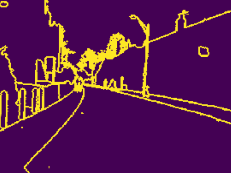
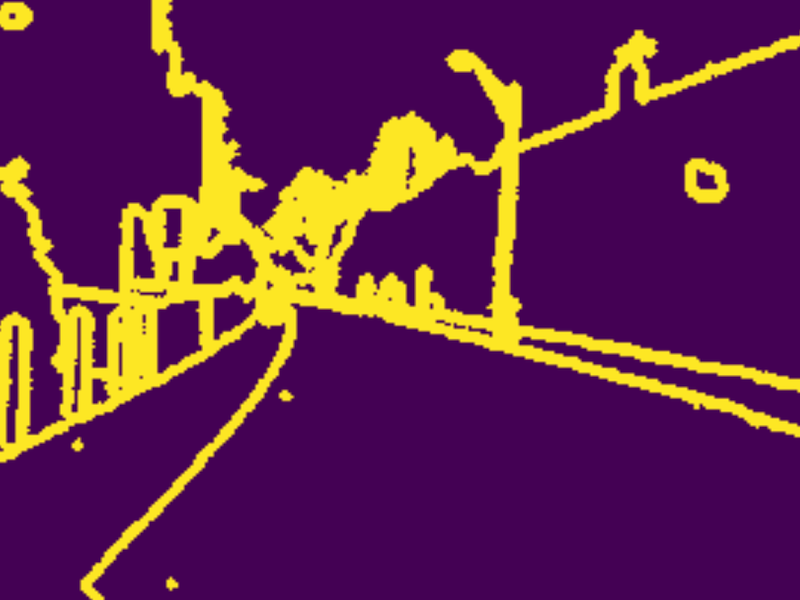
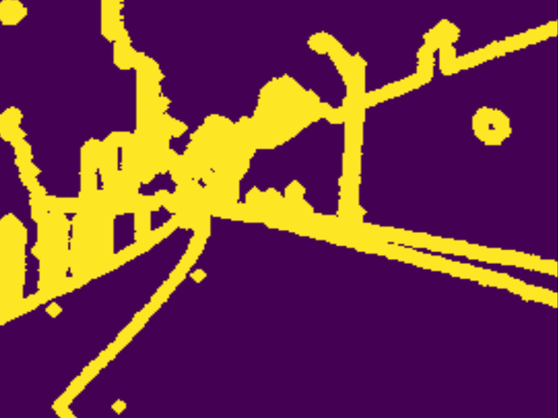
Figure 9: Left to right: 1, 2, 3 border pixel are selected respectively. Frames taken from CamVid dataset.

(a) Influence of border thickness.

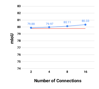
(b) Influence of number of connections.

Figure 10: Influence of graph attributes on mIoU.

# connections	mIoU	Border Thickness	mIoU	# features	mIoU	Dropout Rate	mIoU	Regularization	mIoU
2	79.88	1	80.11	11	78.37	0	80.20	1.00e-01	74.79
4	79.97	2	80.00	15	80.45	0.0001	80.39	1.00e-04	80.12
8	80.11	3	80.16	256	81.12	0.001	80.11	1.00e-08	80.24
16	80.33	4	80.07	271	80.90	0.1	80.09	1.00e-11	80.14
-	-	5	80.10	319	80.99	0.5	80.33	1.00e-13	80.22
-	-	6	79.96	510	81.59	0.9	79.39	-	-
-	-	-	-	1039	81.73	-	-	-	-
-	-	-	-	1999	81.92	-	-	-	-

Table 2: Ablation study with quantitative mIoU values achieved using Border-SegGCN with DeepLabV3+ for Camvid dataset using different number of connections in the graph, number of border pixel thickness, number of features, dropout rate, and regularization

6.3.2 Number of Edges:

As the number of edges is variable, we see how the number of connections each node has influences the results of improving the segmentation task (with the help of improving the border pixel classification). Figure 10b shows that the results steadily increase as the number of edges increases because the more edges a singular node has, the more spatial information it carries about its neighbours. It is also worth mentioning that increasing indefinitely the number of edges has two adverse effects. First, it becomes computationally more expensive to generate the graph as more information is stored per node. But second, and more importantly, the impact of each edge decreases as the number of edges increases.

6.3.3 Number of Features:

The most important consideration within the graph creation process is the feature selection step. The features have to represent enough information to the GCN for it to predict the correct pixel class. Figure 11 represents the correlation between the mean IoU and the number of feature channels.

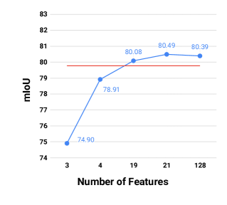
(a) Border-SegGCN with Unet

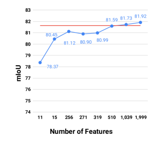
(b) Border-SegGCN with DeepLabV3+

Figure 11: Influence of number of features on the mIoU.

Each step represents a different set of features, representing a combination of different feature sets. Unsurprisingly, the best results are obtained by combining the base algorithm’s output, the intensity values of the frames, and a combination of intermediary layers.

Number of features	Constituent features
3	’I’
4	’base’ + ’I’
19	’RGB’ + ’d5’
21	’base’ + ’I’ + ’seg’ + ’d5’
128	’base’ + ’I’ + ’seg’ + ’d3’ + ’d4’ + ’d5’

Table 3: Decomposition of the features that were used as input to GCN when Unet is a base network in Border-SegGCN. Notations: I-intensity values of the RGB channels, base-output segmented image from base network, d3-d5-last 3 decoder layer of Unet.

Number of features	Constituent features
11	’I’
15	’I’ + ’base’
256	’mba’
271	’base’+’I’+ ’$final_{6}$’+’$final_{3}$’
319	’base’+’I’+ ’seg’+’mba’
510	’I’+ ’$final_{6}$’+’m1+’m2’+’seg’+’mba’
1039	’I’+ ’$final_{6}$’+’m5’
1999	’base’+ ’I’+ ’$final_{6}$’ +’m1’+’m2’+’m3’+’m4’+’m5’

Table 4: Decomposition of the features that were used as input to GCN when DeepLabV3+ is a base network in Border-SegGCN. Notations: I-intensity values of the RGB channels, base-output segmented image from base network, ’$final_{1-6}$’-Segmentation heads sublayers 1 to 6, m1-m7- Encoder layers 1 to 7, ’mba’-Atrous spatial pyramid pooling output

6.3.4 GCN Dropout Optimisation:

We used a modification of the architecture given in [26] that showed an improvement when the number of layers is varied from the original network. We show the dropout effects on the mean IoU score in Figure 12a.

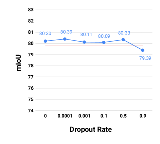
(a) Dropout effect on mIoU

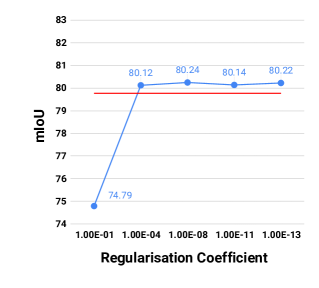
(b) Regularisation effect on mIoU

Figure 12: Influence of dropout and regularisation on Border-SegGCN.

6.3.5 GCN Regularisation Optimisation:

Figure 12b shows the mIoU improvement as the regularisation coefficient decreases. This concludes that the GCN is not prone to overfitting and thus can generalise the results.

6.3.6 Different Base Model: DeepLabV3+:

We use the base network Unet in the previous studies. Recent research shows that there have been architectures that have improved performance over Unet such as the DeepLabV3+ [9].

We observe the same trend with the Unet experiments. When increasing the number of feature channels, mIoU increases as well. However, the amount of features is much higher and requires much more computational resources with this network. Figure 11b suggests that we are capable of improving an output from different models with our architecture pipeline.

6.4 Time Complexity

Total time required for each frame in the video is around 19 seconds. The average time for DeepLabV3+ is 0.08sec per frame. So, Border-SegGCN has a drawback of latency. We are introducing this technique as a stepping stone so that the research can also be focused on GCNs for improving semantic segmentation using improved techniques.

6.5 Image Size

This approach requires adjacency matrix has squared dimension of the given image. So, due to available GPU resources, it is not possible to do experiments on various video segmentation datasets having large frame size.

6.6 Qualitative Results

Figure 13 shows qualitative examples of the output generated by our pipeline. The output segmented frames from using both, the Unet and DeepLabV3+, as base network are illustrated with their best input feature set compared to an under-performing input feature set.

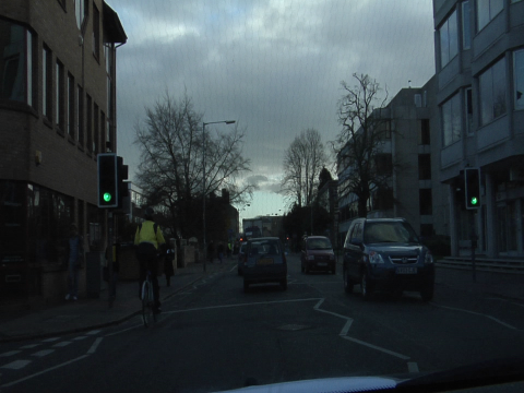
(a)

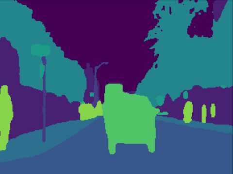
(b)

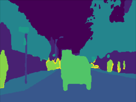
(c)

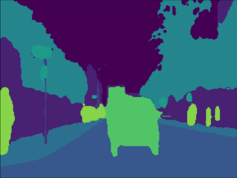
(d)

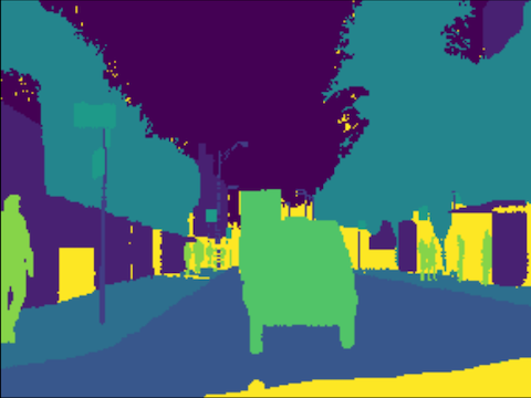
(e)

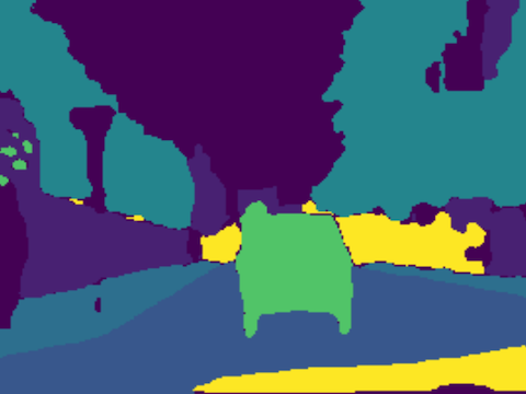
(f)

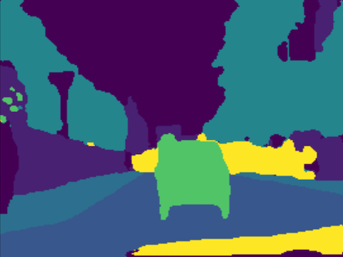
(g)

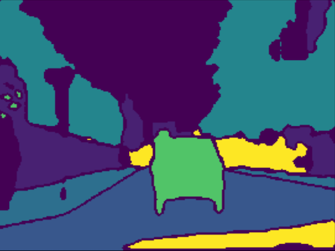
(h)

Figure 13: (a) Original. (b) DeepLabV3+ baseline. (c) Best Border-SegGCN with DeepLabV3+. (d) Poor Border-SegGCN with DeepLabV3+. (e) Ground truth. (f) Unet baseline. (g) Best Border-SegGCN with Unet. (h) Poor Border-SegGCN with Unet.

We noticed from Figure 13 that

• In the case of Unet as shown in Figure 13f, when the model is under-performing due to use of wrong feature set input to the GCN, the model defaults to the statistical most likely category 13h.

• DeepLabV3+ has difficulties with objects that appear smaller in the frame 13b,

• Our model is capable of correcting the DeepLabV3+ predictions on the outline of those objects 13c.

• The outlines using Border-SegGCN in 13g are better defined as compared to 13f.

7 Conclusion

Our proposed model “Border-SegGCN” employs the base segmentation network such as Unet and DeepLabV3+ along with the GCN. Border-SegGCN is used to refine the object boundaries predictions. The most important task for improving the prediction performance of the base algorithm is the feature selection to be used as input to GCN. The variation due to features is the largest contributing factor in both baseline architectures, i.e., Unet and DeepLabV3+. Our experiments showed that Border-SegGCN is agnostic to the choice of baseline model. The more spatial information a node has on its neighbours, expressed by the number of edges, the better is the performance of the GCN. Finally, our experimental results show that the proposed model gives a new state-of-the-art performance on CamVid dataset using DeepLabV3+ as baseline network. It also improved the results of Unet baseline for both Camvid and Carla datasets. In future work, we will work on tackling the drawbacks of this technique, i.e. improving latency, and reducing computation complexity.

References

- [1] Yuri Boykov and Gareth Funka-Lea. Graph cuts and efficient nd image segmentation. International Journal of Computer Vision - IJCV, 70:109–131, 11 2006.
- [2] Gabriel J. Brostow, Julien Fauqueur, and Roberto Cipolla. Semantic object classes in video: A high-definition ground truth database. Pattern Recognition Letters, xx(x):xx–xx, 2008.
- [3] Holger Caesar, Jasper Uijlings, and Vittorio Ferrari. Coco-stuff: Thing and stuff classes in context. In Proceedings of the IEEE Conference on Computer Vision and Pattern Recognition, pages 1209–1218, 2018.
- [4] Camvid - the cambridge-driving labeled video database.
- [5] Siddhartha Chandra and Iasonas Kokkinos. Fast, exact and multi-scale inference for semantic image segmentation with deep gaussian crfs. In European Conference on Computer Vision, pages 402–418. Springer, 2016.
- [6] Siddhartha Chandra, Nicolas Usunier, and Iasonas Kokkinos. Dense and low-rank gaussian crfs using deep embeddings. In Proceedings of the IEEE International Conference on Computer Vision, pages 5103–5112, 2017.
- [7] Liang-Chieh Chen, George Papandreou, Iasonas Kokkinos, Kevin Murphy, and Alan L Yuille. Deeplab: Semantic image segmentation with deep convolutional nets, atrous convolution, and fully connected crfs. IEEE transactions on pattern analysis and machine intelligence, 40(4):834–848, 2017.
- [8] Liang-Chieh Chen, Yukun Zhu, George Papandreou, Florian Schroff, and Hartwig Adam. Encoder-decoder with atrous separable convolution for semantic image segmentation. In Proceedings of the European conference on computer vision (ECCV), pages 801–818, 2018.
- [9] Liang-Chieh Chen, Yukun Zhu, George Papandreou, Florian Schroff, and Hartwig Adam. Encoder-decoder with atrous separable convolution for semantic image segmentation, 2018.
- [10] Marius Cordts, Mohamed Omran, Sebastian Ramos, Timo Rehfeld, Markus Enzweiler, Rodrigo Benenson, Uwe Franke, Stefan Roth, and Bernt Schiele. The cityscapes dataset for semantic urban scene understanding. In Proceedings of the IEEE conference on computer vision and pattern recognition, pages 3213–3223, 2016.
- [11] Jifeng Dai, Kaiming He, and Jian Sun. Convolutional feature masking for joint object and stuff segmentation. In Proceedings of the IEEE conference on computer vision and pattern recognition, pages 3992–4000, 2015.
- [12] Naina Dhingra and Andreas Kunz. Res3atn-deep 3d residual attention network for hand gesture recognition in videos. In 2019 International Conference on 3D Vision (3DV), pages 491–501. IEEE, 2019.
- [13] Alexey Dosovitskiy, German Ros, Felipe Codevilla, Antonio Lopez, and Vladlen Koltun. Carla: An open urban driving simulator. In Conference on robot learning. PMLR, 2017.
- [14] David K Duvenaud, Dougal Maclaurin, Jorge Iparraguirre, Rafael Bombarell, Timothy Hirzel, Alán Aspuru-Guzik, and Ryan P Adams. Convolutional networks on graphs for learning molecular fingerprints. In Advances in neural information processing systems, pages 2224–2232, 2015.
- [15] David Eigen and Rob Fergus. Predicting depth, surface normals and semantic labels with a common multi-scale convolutional architecture. In Proceedings of the IEEE international conference on computer vision, pages 2650–2658, 2015.
- [16] Mark Everingham, SM Ali Eslami, Luc Van Gool, Christopher KI Williams, John Winn, and Andrew Zisserman. The pascal visual object classes challenge: A retrospective. International journal of computer vision, 111(1):98–136, 2015.
- [17] Mark Everingham, Luc Van Gool, Christopher KI Williams, John Winn, and Andrew Zisserman. The pascal visual object classes (voc) challenge. International journal of computer vision, 88(2):303–338, 2010.
- [18] Clement Farabet, Camille Couprie, Laurent Najman, and Yann LeCun. Learning hierarchical features for scene labeling. IEEE transactions on pattern analysis and machine intelligence, 35(8):1915–1929, 2012.
- [19] Xiang Gao, Wei Hu, Jiaxiang Tang, Jiaying Liu, and Zongming Guo. Optimized skeleton-based action recognition via sparsified graph regression. In Proceedings of the 27th ACM International Conference on Multimedia, pages 601–610, 2019.
- [20] Stephen Gould, Richard Fulton, and Daphne Koller. Decomposing a scene into geometric and semantically consistent regions. In 2009 IEEE 12th international conference on computer vision, pages 1–8. IEEE, 2009.
- [21] Xuming He, Richard S Zemel, and Miguel Á Carreira-Perpiñán. Multiscale conditional random fields for image labeling. In Proceedings of the 2004 IEEE Computer Society Conference on Computer Vision and Pattern Recognition, 2004. CVPR 2004., volume 2, pages II–II. IEEE, 2004.
- [22] Mikael Henaff, Joan Bruna, and Yann LeCun. Deep convolutional networks on graph-structured data. arXiv preprint arXiv:1506.05163, 2015.
- [23] Varun Jampani, Martin Kiefel, and Peter V Gehler. Learning sparse high dimensional filters: Image filtering, dense crfs and bilateral neural networks. In Proceedings of the IEEE Conference on Computer Vision and Pattern Recognition, pages 4452–4461, 2016.
- [24] Guillaume Jaume, Behzad Bozorgtabar, Hazim Kemal Ekenel, Jean-Philippe Thiran, and Maria Gabrani. Image-level attentional context modeling using nested-graph neural networks. arXiv preprint arXiv:1811.03830, 2018.
- [25] Diederik P Kingma and Jimmy Ba. Adam: A method for stochastic optimization. arXiv preprint arXiv:1412.6980, 2014.
- [26] Thomas N. Kipf and Max Welling. Semi-supervised classification with graph convolutional networks. CoRR, abs/1609.02907, 2016.
- [27] Alex Krizhevsky, Ilya Sutskever, and Geoffrey E Hinton. Imagenet classification with deep convolutional neural networks. In Advances in neural information processing systems, pages 1097–1105, 2012.
- [28] L’ubor Ladickỳ, Chris Russell, Pushmeet Kohli, and Philip HS Torr. Associative hierarchical crfs for object class image segmentation. In 2009 IEEE 12th International Conference on Computer Vision, pages 739–746. IEEE, 2009.
- [29] Guohao Li, Matthias Muller, Ali Thabet, and Bernard Ghanem. Deepgcns: Can gcns go as deep as cnns? In Proceedings of the IEEE International Conference on Computer Vision, pages 9267–9276, 2019.
- [30] Maosen Li, Siheng Chen, Xu Chen, Ya Zhang, Yanfeng Wang, and Qi Tian. Actional-structural graph convolutional networks for skeleton-based action recognition. In Proceedings of the IEEE Conference on Computer Vision and Pattern Recognition, pages 3595–3603, 2019.
- [31] Ruiyu Li, Makarand Tapaswi, Renjie Liao, Jiaya Jia, Raquel Urtasun, and Sanja Fidler. Situation recognition with graph neural networks. In Proceedings of the IEEE International Conference on Computer Vision, pages 4173–4182, 2017.
- [32] Yi Li, Haozhi Qi, Jifeng Dai, Xiangyang Ji, and Yichen Wei. Fully convolutional instance-aware semantic segmentation. In Proceedings of the IEEE Conference on Computer Vision and Pattern Recognition, pages 2359–2367, 2017.
- [33] Di Lin, Jifeng Dai, Jiaya Jia, Kaiming He, and Jian Sun. Scribblesup: Scribble-supervised convolutional networks for semantic segmentation. In Proceedings of the IEEE Conference on Computer Vision and Pattern Recognition, pages 3159–3167, 2016.
- [34] Guosheng Lin, Chunhua Shen, Anton Van Den Hengel, and Ian Reid. Efficient piecewise training of deep structured models for semantic segmentation. In Proceedings of the IEEE conference on computer vision and pattern recognition, pages 3194–3203, 2016.
- [35] Tsung-Yi Lin, Michael Maire, Serge Belongie, James Hays, Pietro Perona, Deva Ramanan, Piotr Dollár, and C Lawrence Zitnick. Microsoft coco: Common objects in context. In European conference on computer vision, pages 740–755. Springer, 2014.
- [36] Rong Liu, Chunyan Xu, Tong Zhang, Wenting Zhao, Zhen Cui, and Jian Yang. Si-gcn: Structure-induced graph convolution network for skeleton-based action recognition. In 2019 International Joint Conference on Neural Networks (IJCNN), pages 1–8. IEEE, 2019.
- [37] Federico Monti, Michael Bronstein, and Xavier Bresson. Geometric matrix completion with recurrent multi-graph neural networks. In Advances in Neural Information Processing Systems, pages 3697–3707, 2017.
- [38] Mohammadreza Mostajabi, Payman Yadollahpour, and Gregory Shakhnarovich. Feedforward semantic segmentation with zoom-out features. In Proceedings of the IEEE conference on computer vision and pattern recognition, pages 3376–3385, 2015.
- [39] Lichao Mou, Yuansheng Hua, and Xiao Xiang Zhu. A relation-augmented fully convolutional network for semantic segmentation in aerial scenes. In Proceedings of the IEEE conference on computer vision and pattern recognition, pages 12416–12425, 2019.
- [40] Pedro O. Pinheiro and Ronan Collobert. Recurrent convolutional neural networks for scene labeling. In 31st International Conference on Machine Learning (ICML), pages 82–90, 2014.
- [41] Xiaojuan Qi, Renjie Liao, Jiaya Jia, Sanja Fidler, and Raquel Urtasun. 3d graph neural networks for rgbd semantic segmentation. In Proceedings of the IEEE International Conference on Computer Vision, pages 5199–5208, 2017.
- [42] Guocheng Qian, Abdulellah Abualshour, Guohao Li, Ali Thabet, and Bernard Ghanem. Pu-gcn: Point cloud upsampling using graph convolutional networks. arXiv preprint arXiv:1912.03264, 2019.
- [43] Kate Rakelly, Evan Shelhamer, Trevor Darrell, Alyosha Efros, and Sergey Levine. Conditional networks for few-shot semantic segmentation. In 6th International Conference on Learning Representations, 2018.
- [44] Olaf Ronneberger, Philipp Fischer, and Thomas Brox. U-net: Convolutional networks for biomedical image segmentation. In International Conference on Medical image computing and computer-assisted intervention, pages 234–241. Springer, 2015.
- [45] Samuel Rota Bulò, Lorenzo Porzi, and Peter Kontschieder. In-place activated batchnorm for memory-optimized training of dnns. In Proceedings of the IEEE Conference on Computer Vision and Pattern Recognition, pages 5639–5647, 2018.
- [46] Alexander G Schwing and Raquel Urtasun. Fully connected deep structured networks. arXiv preprint arXiv:1503.02351, 2015.
- [47] Chenyang Si, Wentao Chen, Wei Wang, Liang Wang, and Tieniu Tan. An attention enhanced graph convolutional lstm network for skeleton-based action recognition. In Proceedings of the IEEE Conference on Computer Vision and Pattern Recognition, pages 1227–1236, 2019.
- [48] Martin Simonovsky and Nikos Komodakis. Dynamic edge-conditioned filters in convolutional neural networks on graphs. In Proceedings of the IEEE conference on computer vision and pattern recognition, pages 3693–3702, 2017.
- [49] Raviteja Vemulapalli, Oncel Tuzel, Ming-Yu Liu, and Rama Chellapa. Gaussian conditional random field network for semantic segmentation. In Proceedings of the IEEE conference on computer vision and pattern recognition, pages 3224–3233, 2016.
- [50] Rui Wang, Chenyang Huang, and Xiangyang Wang. Global relation reasoning graph convolutional networks for human pose estimation. IEEE Access, 2020.
- [51] Zonghan Wu, Shirui Pan, Fengwen Chen, Guodong Long, Chengqi Zhang, and Philip S Yu. A comprehensive survey on graph neural networks. arXiv preprint arXiv:1901.00596, 2019.
- [52] Chunyu Xie, Ce Li, Baochang Zhang, Chen Chen, Jungong Han, Changqing Zou, and Jianzhuang Liu. Memory attention networks for skeleton-based action recognition. arXiv preprint arXiv:1804.08254, 2018.
- [53] Keyulu Xu, Weihua Hu, Jure Leskovec, and Stefanie Jegelka. How powerful are graph neural networks? arXiv preprint arXiv:1810.00826, 2018.
- [54] Qiangeng Xu. Grid-gcn for fast and scalable point cloud learning. arXiv preprint arXiv:1912.02984, 2019.
- [55] Pavel Yakubovskiy. Segmentation models pytorch. https://github.com/qubvel/segmentation$_$models.pytorch, 2020.
- [56] Sijie Yan, Yuanjun Xiong, and Dahua Lin. Spatial temporal graph convolutional networks for skeleton-based action recognition. In Thirty-second AAAI conference on artificial intelligence, 2018.
- [57] Jian Yao, Sanja Fidler, and Raquel Urtasun. Describing the scene as a whole: Joint object detection, scene classification and semantic segmentation. In 2012 IEEE conference on computer vision and pattern recognition, pages 702–709. IEEE, 2012.
- [58] Jian Zhang, Josip Djolonga, and Andreas Krause. Higher-order inference for multi-class log-supermodular models. In International Conference on Computer Vision (ICCV), December 2015.
- [59] Muhan Zhang and Yixin Chen. Link prediction based on graph neural networks. In Advances in Neural Information Processing Systems, pages 5165–5175, 2018.
- [60] Yiheng Zhang, Zhaofan Qiu, Ting Yao, Dong Liu, and Tao Mei. Fully convolutional adaptation networks for semantic segmentation. In Proceedings of the IEEE Conference on Computer Vision and Pattern Recognition, pages 6810–6818, 2018.
- [61] Long Zhao, Xi Peng, Yu Tian, Mubbasir Kapadia, and Dimitris N Metaxas. Semantic graph convolutional networks for 3d human pose regression. In Proceedings of the IEEE Conference on Computer Vision and Pattern Recognition, pages 3425–3435, 2019.
- [62] Yin Zheng, Dongping Zhang, Li Yang, and Zhihong Zhou. Fall detection and recognition based on gcn and 2d pose. In 2019 6th International Conference on Systems and Informatics (ICSAI), pages 558–562. IEEE, 2019.
- [63] Yi Zhu, Karan Sapra, Kevin J. Shih Fitsum A. Reda, Shawn Newsam, Andrew Tao, and Bryan Catanzaro. Improving semantic segmentation via video propagation and label relaxation. In IEEE Conference on Computer Vision and Pattern Recognition (CVPR), June 2019.