Class-Distribution-Aware Calibration for Long-Tailed Visual Recognition

Abstract

Despite impressive accuracy, deep neural networks are often miscalibrated and tend to overly confident predictions. Recent techniques like temperature scaling (TS) and label smoothing (LS) show effectiveness in obtaining a well-calibrated model by smoothing logits and hard labels with scalar factors, respectively. However, the use of uniform TS or LS factor may not be optimal for calibrating models trained on a long-tailed dataset where the model produces overly confident probabilities for high-frequency classes. In this study, we propose class-distribution-aware TS (CDA-TS) and LS (CDA-LS) by incorporating class frequency information in model calibration in the context of long-tailed distribution. In CDA-TS, the scalar temperature value is replaced with the CDA temperature vector encoded with class frequency to compensate for the over-confidence. Similarly, CDA-LS uses a vector smoothing factor and flattens the hard labels according to their corresponding class distribution. We also integrate CDA optimal temperature vector with distillation loss, which reduces miscalibration in self-distillation (SD). We empirically show that class-distribution-aware TS and LS can accommodate the imbalanced data distribution yielding superior performance in both calibration error and predictive accuracy. We also observe that SD with an extremely imbalanced dataset is less effective in terms of calibration performance. Code is available in https://github.com/mobarakol/Class-Distribution-Aware-TS-LS.

1 Introduction

Modern deep neural networks have demonstrated the ability to achieve very high accuracy in recognition tasks. These deeper and wider networks can fit the training dataset with ease, achieving high accuracy (Zhang et al., 2016). However, this raises a new concern, to what extend the network’s predictions are likely to be correct? As these deep network tries to reduce the negative log-likelihood loss, they overfit to datasets, rendering its predictions to be over-confident and less trustworthy (Mukhoti et al., 2020). Here, the network is termed to be poorly calibrated. In a calibrated model, the accuracy matches the prediction confidence. A well-calibrated model is of utmost importance in a real-world application, at times assisting the user make a life-saving decision. For instance, letting the doctor decide whether to perform further diagnosis should the model’s predictions be of low confidence. Network miscalibration is strongly related to the network’s expanding capacity and the lack of regularization techniques (Guo et al., 2017). Additionally, the long-tailed dataset has also been found to cause model miscalibration. As the dataset distribution is biased towards few very significant classes, in reducing the training loss, the model’s predictions get over-confident towards these classes, leading to model miscalibration (see Appendix A.2, Figure 4). This creates additional issues in calibrating probability prediction with conventional calibration methods.

The importance of model calibration over model accuracy has been acknowledged and worked upon recently. Most frequent methods used for model calibration are Platt scaling (Platt, 1999), isotonic regression (Niculescu-Mizil & Caruana, 2005) and, bayesian binning and averaging (Bella et al., 2009). Temperature scaling (TS), a variant of Platt scaling, has been proven to have a positive effect in calibrating the model (Guo et al., 2017). In the temperature scaling technique, the network’s confidence in its prediction is scaled down by diving the logits with a scalar value, called the temperature scale (T $>$ 0). The scaled logits help overcome the problem of overconfidence and thereby attaining better model calibration.

Most recently, label smoothing (LS) is introduced, a regularization technique to flatten the hard onehot label to improve accuracy, thereby implicitly reduces the overconfident predictions and demonstrate better confident calibration and feature representation (Müller et al., 2019). A scalar smoothing factor controls the smoothing level where a higher value enforces a larger squeeze in the true label.

Despite the effective performance of TS and LS in probability calibration with the standard dataset, there are additional issues with a long-tailed dataset where the distribution of a few classes is significantly higher than the other. In reality, most sensitive applications do not possess a balanced dataset. Therefore, during training, the model gets biased towards reducing the loss of the few high-frequency classes, thereby causing over-confidence and miscalibration. In both techniques, TS and LS, a scalar smoothing factor applied uniformly over all the classes do not cater to probability prediction biases introduced by class distribution. In this work, we propose Class-Distribution-Aware TS (CDA-TS) and LS (CDA-LS) that incorporates class frequency information to calibrate prediction probability in the long-tailed dataset.

The key contributions of this paper are as follows:(I) We introduce a class-distribution-aware temperature scaling (CDA-TS) and label smoothing (CDA-LS) techniques that improve model calibration despite training on the long-tailed datasets; (II) We design a knowledge-distillation (KD) loss with CDA-TS and demonstrate the superior performance of our KD loss in self-distillation; (III) We validate the effectiveness of our methods on three long-tailed datasets and four state-of-the-art probability calibration metrics, uncertainty calibration metric and reliability diagrams.

2 Method

2.1 Preliminaries

Most of the model calibration techniques try to reduce the over-confident prediction by manipulating either onehot label or predicted probability. For example, temperature scaling (TS) downgrades the logits by dividing them using a scalar temperature value and label smoothing (LS) squeezes the onehot label with a scalar smoothing factor. In TS, temperature scaled probability is $\hat{P}^{TS}=\sigma_{SM}(z/T)$, where temperature $T$ ($>1$), logits $z$ and softmax layer $\sigma_{SM}$. To find the optimal temperature, a conjugate gradient solver or a naive line-search is used on a trained model without affecting model accuracy (Guo et al., 2017). In LS, smoothened label or soft label is $P^{LS}=P^{OH}(1-\alpha)+\alpha/N$, where smoothing factor $\alpha$ ($0<1$), onehot label $P^{OH}$ and total number of classes $N$. The smoothing factor $\alpha$ controls the flatten degree in the smoothened label. A higher value provides a larger smoothened label. This is also called soft labels ($P^{LS}$) and used to calculate CE loss, $L_{CE}=\sum_{c=1}^{N}-{P^{LS}_{c}}log({\hat{P}_{c})}$, where $\hat{P}_{c})$ is the predicted probability. Though both TS and LS are proven to improve model calibration to an extend, model miscalibration is not entirely addressed since it can be affected by long-tailed distribution.

2.2 Class-Distribution-Aware TS

TS addresses model miscalibration by dividing the logits with an optimal temperature value. By scaling the logits, TS restricts the model from being overly confident in its prediction. The TS scales all the logits using a scalar value uniformly. However, a model trained on a long-tailed dataset could be biased towards high-frequency classes, resulting in overly confident logits. There, we introduce a class-distribution-aware TS (CDA-TS) that incorporates class frequency information with the optimal temperature. We construct a vector temperature instead of a scalar by re-weighting the optimal temperature based on class frequency in the dataset. In this way, high-frequency classes divide with a larger value of the temperature and substantially downgrade the confidence score.

If [$f_{1},f_{2},...f_{N}$] are the max-normalized class frequencies for N total classes and $T^{opt}$ is the optimal temperature then class-distribution-aware vector temperature $T^{cda}$ formulates is defined as:

$$T^{cda}=T^{opt}+\gamma[f_{1},f_{2},...,f_{N}]$$ (1)

where, $\gamma$ is the down-scale factor and the suitable value of $\gamma=0.1$ is found by the experiments. Therefore, the final equation of CDA temperature scaling is $\hat{P}^{CDA-TS}=\sigma_{SM}([z_{1},z_{2},...,z_{N}]/[T^{cda}_{1},T^{cda}_{2},...,T^{cda}_{N}])$.

Table 1: Performance of Class-aware TS on CIFAR-100-LT, Places-LT and ImageNet-LT dataset with ResNet18, ResNet152 and ResNet10, respectively.

Dataset	Ratio	Method	ACC$\uparrow$	ECE$\downarrow$	SCE$\downarrow$	TACE$\downarrow$	BS$\downarrow$	UCE$\downarrow$
CIFAR-100-LT	10	Baseline	57.60	0.1801	0.0047	0.0043	0.6115	0.2344
		TS (1.551)	57.60	0.0425	0.0034	0.0035	0.5656	0.0502
		CDA-TS	57.93	0.0356	0.0032	0.0033	0.5593	0.0305
	100	Baseline	38.57	0.3280	0.0082	0.0071	0.8976	0.3892
		TS (2.0147)	38.57	0.0372	0.0047	0.0056	0.7580	0.0194
		CDA-TS	38.90	0.0280	0.0046	0.0055	0.7526	0.0099
Places-LT	996	Baseline	29.34	0.2987	0.0022	0.0019	0.9590	0.4512
		TS (1.7349)	29.34	0.0619	0.0014	0.0016	0.8505	0.1760
		CDA-TS	29.63	0.0581	0.0014	0.0016	0.8467	0.1689
ImageNet-LT	256	Baseline	34.83	0.0853	0.0007	0.0006	0.7976	0.2850
		TS (1.1200)	34.83	0.0348	0.0006	0.0006	0.7897	0.2301
		CDA-TS	35.68	0.0214	0.0006	0.0006	0.7795	0.2116

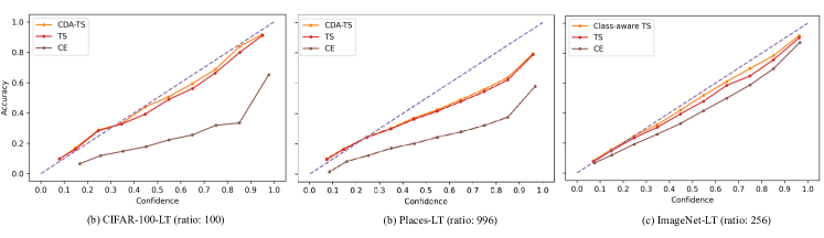
Figure 1: Reliability graph for CE, TS and CDA-TS with (a) CIFAR-100-LT imbalanced ratio of 100, (b) Places-LT imbalanced ratio of 996 and (c) ImageNet-LT imbalanced ratio of 256.

2.3 Class-Distribution-Aware LS

Label smoothing (LS) limits the network to produce overly confident predictions by squeezing the true onehot label in CE loss calculation. In LS, onehot label flattens with a uniform distribution by using a smoothing factor. However, high-frequency classes in the long-tailed dataset overfit the model, limiting the LS performance with a uniform smoothing factor. To tackle this problem, we generate a class-distribution-aware LS (CDA-LS) soothing factor and replace the scalar smoothing factor in training with LS. CDA-LS flatten the high-frequency classes with a higher penalty than low-frequency classes. Similar to CDA-TS, the class-distribution-aware smoothing factor can be formulated as:

$$\alpha^{cda}=\alpha+\gamma[f_{1},f_{2},...,f_{N}]$$ (2)

where, the down-scale factor $\gamma=0.01$ is found by the experiments. Therefore, soft labels can be generated as, $P^{CDA-LS}=P^{OH}(1-[\alpha^{cda}_{1},\alpha^{cda}_{2},...,\alpha^{cda}_{N}])+[\alpha^{cda}_{1},\alpha^{cda}_{2},...,\alpha^{cda}_{N}]/N$.

2.4 Self-Distillation with CDA-TS

A popular way to use knowledge distillation (KD) (as well as self-distillation(SD)) is to apply Kullback-Leibler divergence loss on temperature (T) scaled logits of teacher and student model (Hinton et al., 2015). A predefined value of T (e.g., $T=4$) is used to produces a softer probability distribution over the classes while calculating KD loss. Nevertheless, a long-tailed dataset produces overly confident probability to certain classes, and a fixed value of T is not tackling the long-tail effect during KD. Similar to CDA-TS, the information of class distribution can be integrated with the T in KD loss and formulated as-

$$L_{SD}=\sum_{c=1}^{N}\mathrm{KL}\Big{(}\sigma_{SM}\big{(}\frac{z^{t}(c)}{T^{cda}(c)}\big{)},\sigma_{SM}\big{(}\frac{z^{s}(c)}{T^{cda}(c)}\big{)}\Big{)}$$ (3)

where $T^{cda}(c)$ is the CDA temperature for $c^{th}$ class and $z^{t}$, $z^{s}$ are the logits of teacher and student network, respectively. Student loss ($L_{CE}$) and distillation loss ($L_{SD}$) are fused to train the student model.

3 Experiments

3.1 Dataset

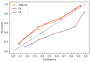
Figure 2: Reliability graph for CE, LS and class-aware LS with CIFAR-100-LT imbalanced ratio of 10.

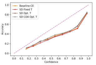
Figure 3: Reliability diagram for baseline-CE, SD with Fixed T and class-distribution-aware T with CIFAR-100-LT imbalanced ratio of 10.

The experiments are conducted on three long-tailed datasets: CIFAR-100-LT (Krizhevsky et al., 2009), Places-LT (Zhou et al., 2017) and ImageNet-LT (Liu et al., 2019). CIFAR-100-LT: The 100-class CIFAR-100 long-tailed dataset is generated by following (Cao et al., 2019) with a data distribution imbalance factor of 10 and 100. Places-LT: The 365-class Places long-tailed dataset with aa imbalance factor of 996 from (Ren et al., 2020) is adopted. The dataset consists of $62.5$k training images and $36.5$k test images. ImageNet-LT: similar to Places-LT dataset, the 1000-class ImageNet dataset with an imbalance factor of 256 is also adopted from (Ren et al., 2020). The dataset comprises $115$k training images and $20$k test images.

3.2 Implementation

The two CIFAR-100-LT with the 10 and 100 imbalance factor are trained on ResNet18 (Zhang et al., 2017) backbone. The model is trained using an SGD optimizer with a batch size of 1024, a momentum of $0.9$, the number of train epochs of 200 and a learning rate of $0.1$. For Places-LT and ImageNet-LT dataset, pre-trained ResNet152 and ResNet18 models from (Ren et al., 2020) are used, respectively. Cross-entropy (CE) loss is employed in training all the backbone networks.

4 Evaluation

The model’s performance and its miscalibration are quantified using accuracy (ACC) and various state-of-the-art calibration error metrics such as Expected calibration error (ECE) (Guo et al., 2017; Naeini et al., 2015), Static calibration error (SCE), thresholded adaptive calibration error (TACE), brier score (BS) (Nixon et al., 2019; Ashukha et al., 2020) and uncertainty calibration error (UCE)  (Laves et al., 2019) (see Appendix B).

As shown in Table 1, the proposed CDA-TS is observed to outperform both the (a) baseline and (b) TS calibrated model and improve model calibration in all three long-tailed datasets. Reliability is also showing better calibration with CDA-TS in Figure 1, bringing the confidence curve close to an identify function. The proposed CDA-LS is also observed to improve model calibration compared to baselines in Table 2 and Figure 2. On the other hand, SD based on CDA optimal T outperforms (a) base model and (b) SD based on fixed T (Hinton et al., 2015) in improving accuracy and model calibration (as shown in Table 3) and Figure 3.

Table 2: Performance of class-aware LS on CIFAR-100-LT dataset. LS smoothing factor $\alpha=0.1$ is assigned for all the experiments.

	Imb. Ratio: 10			Imb. Ratio: 100
	ACC	ECE	UCE	ACC	ECE	UCE
Baseline	57.60	0.180	0.234	38.57	0.328	0.389
LS	57.98	0.092	0.153	37.90	0.045	0.040
CDA-LS	58.35	0.078	0.137	37.94	0.038	0.047

Table 3: CIFAR-100-LT performance of Class-distribution-aware TS on self-distillation with fixed temperature is set to 4 and optimal (opt.) temperature obtains 1.551 for the imbalanced ratio of 10.

Method	ACC$\uparrow$	ECE$\downarrow$	TACE$\downarrow$	UCE$\downarrow$
Baseline	57.60	0.1801	0.0043	0.2344
SD (4)	57.64	0.1974	0.0044	0.2498
SD Opt. T (1.551)	57.95	0.1714	0.0042	0.2264
SD CDA Opt. T	58.67	0.1694	0.0042	0.2230

5 Discussion and Conclusion

We have shown that the calibration of a model trained on a long-tailed dataset can be improved by employing class-distribution-aware temperature scaling (CDA-TS) and label-smoothing (CDA-TS). CDA-TS has shown improvement across accuracy and all calibration error matrix of models trained on CIFAR-100-LT, Places-LT and ImageNet-LT. While the proposed CDA-LS technique outperformed the traditional LS techniques in most of the metrics, the scalar LS techniques seem to perform better on other uncertainty calibration error metrics for high imbalance factor (as in Table 2). Furthermore, we show that the CDA-TS does not hinder knowledge distillation. It outperforms the baseline model and model trained using TS in accuracy (as in Table 3). It is observed that, while the use of TS generally increased calibration error when trained on highly imbalanced data, the proposed CDA-TS introduces lesser error compared to the TS technique.

Overall, we have shown that, by incorporating knowledge on class distribution, the CDA-TS and CDA-LS improve model calibration. Additionally, LS is known to hinders knowledge distillation (Müller et al., 2019; Shen et al., 2021). Therefore, we further extend our work and show that CDA-TS improves accuracy and introduce lesser calibration error during knowledge distillation. In the future, we aim to study the effects of CDA calibration techniques in domain adaptation and introduce CDA loss function to improve model accuracy and calibration simultaneously.

Appendix A Related Work

A.1 Network Calibration

Several techniques are being introduced for calibrating networks trained on datasets with the less biased class distribution. The common methods are temperature scaling, isotonic regression, deep ensemble, label smoothing, and mixup. Guo et al. (2017) show that modern neural network is poorly calibrated, and temperature scaling (TS) is effective in calibration prediction. Variants of TS are also being explored. TS is extended to drop-out variational inference to produce well-calibrated model uncertainty (Laves et al., 2019). Local temperature scaling is developed by focusing on calibration in multi-label semantic segmentation (Ding et al., 2020). Other variations of TS include attended temperature scaling (Mozafari et al., 2018), bin-wise temperature scaling (Ji et al., 2019) and TS with focal loss (Mukhoti et al., 2020). Dirichlet calibration, a multiclass calibration method, is introduced using Dirichlet distribution (Kull et al., 2019). Recently, label smoothing presents as one of the efficient regularization techniques to improve the confidence calibration and feature representation (Müller et al., 2019; Islam et al., 2020).

Figure 4: Relation of class-frequency-distribution and corresponding confidence score on CIFAR-100-LT.

A.2 Long-Tailed Dataset

Long-tail is the common issue for pragmatic deep learning applications, consisting of extremely imbalanced class distribution in the training dataset (see Figure 4). There are three general approaches to tackle long-tailed dataset, (a) re-sampling (Byrd & Lipton, 2019; Buda et al., 2018), (b) Re-weighting (Huang et al., 2019), and (c) incorporating class frequency information (Cao et al., 2019; Ren et al., 2020). We are particularly interested in class frequency-based techniques in this work. Label distribution aware margin Loss is introduced to learn the imbalanced dataset in visual classification tasks (Cao et al., 2019). Balanced meta-softmax is designed with class distribution and meta-learning (Ren et al., 2020) where balanced group softmax trains the model group-wise to balance the classifier.

A.3 Self-Distillation

Self-distillation (SD) or knowledge distillation (KD) is a kind of transfer of knowledge from a teacher model to a student model by commonly minimizing an objective function (Ba & Caruana, 2013; Crowley et al., 2018). A popular way to do this is by calculating the Kullback-Leibler divergence loss between the temperature scaled probability of teacher and student models (Hinton et al., 2015). Hardmax and softmax with temperature are used to perform self distillation for overparameterized neural network (Dong et al., 2019).

Appendix B Calibration Metrics

The model’s performance and its miscalibration are quantified using various state-of-the-art calibration error metrics. Expected calibration error (ECE) (Guo et al., 2017; Naeini et al., 2015) is used as the base calibration metric. ECE computes the discrepancy between accuracy and confidence probability. It can be formulate as, $ECE=\sum\limits_{b=1}^{B}\frac{n_{[b]}}{N}\mid Acc_{[b]}-Conf_{[b]}\mid$, where $B$, $N$, $n_{[}b]$, $Acc_{[b]}$ and $Conf_{[b]}$ are the total number of bins, total number of samples, and number of samples, accuracy and confidences in $b^{th}$ bin. However, it is indicated that ECE is sensitive to bin number and unable to present class-wise model calibration (Nixon et al., 2019). Static calibration error (SCE), thresholded adaptive calibration error (TACE), brier score (BS) are introduced to deal with the limitation of ECE and determine accurate calibration error (Nixon et al., 2019; Ashukha et al., 2020). TACE can be formulated as $TACE=\frac{1}{KR}\sum\limits_{k=1}^{K}\sum\limits_{r=1}^{R}\mid Acc_{[r,c]}-Conf_{[r,c]}\mid$, where $R$ is a number of calibration ranges with threshold t, $Acc_{[r,c]}$ and $Conf_{[r,c]}$ are the accuracy and confidence in r range and c class. We also calculate the uncertainty calibration error (UCE) by following (Laves et al., 2019). The formula for UCE is similar to ECE except determining uncertainty calibration instead of probability calibration. Therefore, $UCE=\sum\limits_{b=1}^{B}\frac{n_{[b]}}{N}\mid Err_{[b]}-Uncert_{[b]}\mid$ where, total bin is B, number of samples in $b^{th}$ bin is $n_{[b]}$ and error and uncertainty in the corresponding bin are $Err_{[b]}$ and $Uncert_{[b]}$ respectively. For simplicity we assigned bin size of 10 for all the calibration metrics and threshold of $10^{-3}$ for TACE. The reliability diagram is used to visualize the model’s miscalibration for under-confidence or over-confidence.

References

- Ashukha et al. (2020) Ashukha, A., Lyzhov, A., Molchanov, D., and Vetrov, D. Pitfalls of in-domain uncertainty estimation and ensembling in deep learning. arXiv preprint arXiv:2002.06470, 2020.
- Ba & Caruana (2013) Ba, L. J. and Caruana, R. Do deep nets really need to be deep? arXiv preprint arXiv:1312.6184, 2013.
- Bella et al. (2009) Bella, A., Ferri, C., Hernández-Orallo, J., and Ramírez-Quintana, M. J. Similarity-binning averaging: a generalisation of binning calibration. In International Conference on Intelligent Data Engineering and Automated Learning, pp. 341–349. Springer, 2009.
- Buda et al. (2018) Buda, M., Maki, A., and Mazurowski, M. A. A systematic study of the class imbalance problem in convolutional neural networks. Neural Networks, 106:249–259, 2018.
- Byrd & Lipton (2019) Byrd, J. and Lipton, Z. What is the effect of importance weighting in deep learning? In International Conference on Machine Learning, pp. 872–881. PMLR, 2019.
- Cao et al. (2019) Cao, K., Wei, C., Gaidon, A., Arechiga, N., and Ma, T. Learning imbalanced datasets with label-distribution-aware margin loss. arXiv preprint arXiv:1906.07413, 2019.
- Crowley et al. (2018) Crowley, E. J., Gray, G., and Storkey, A. J. Moonshine: Distilling with cheap convolutions. In NeurIPS, pp. 2893–2903, 2018.
- Ding et al. (2020) Ding, Z., Han, X., Liu, P., and Niethammer, M. Local temperature scaling for probability calibration. arXiv preprint arXiv:2008.05105, 2020.
- Dong et al. (2019) Dong, B., Hou, J., Lu, Y., and Zhang, Z. Distillation approx early stopping? harvesting dark knowledge utilizing anisotropic information retrieval for overparameterized neural network. arXiv preprint arXiv:1910.01255, 2019.
- Guo et al. (2017) Guo, C., Pleiss, G., Sun, Y., and Weinberger, K. Q. On calibration of modern neural networks. In International Conference on Machine Learning, pp. 1321–1330. PMLR, 2017.
- Hinton et al. (2015) Hinton, G., Vinyals, O., and Dean, J. Distilling the knowledge in a neural network. arXiv preprint arXiv:1503.02531, 2015.
- Huang et al. (2019) Huang, C., Li, Y., Loy, C. C., and Tang, X. Deep imbalanced learning for face recognition and attribute prediction. IEEE transactions on pattern analysis and machine intelligence, 42(11):2781–2794, 2019.
- Islam et al. (2020) Islam, M., Seenivasan, L., Ming, L. C., and Ren, H. Learning and reasoning with the graph structure representation in robotic surgery. In International Conference on Medical Image Computing and Computer-Assisted Intervention, pp. 627–636. Springer, 2020.
- Ji et al. (2019) Ji, B., Jung, H., Yoon, J., Kim, K., et al. Bin-wise temperature scaling (bts): Improvement in confidence calibration performance through simple scaling techniques. In 2019 IEEE/CVF International Conference on Computer Vision Workshop (ICCVW), pp. 4190–4196. IEEE, 2019.
- Krizhevsky et al. (2009) Krizhevsky, A., Hinton, G., et al. Learning multiple layers of features from tiny images. 2009.
- Kull et al. (2019) Kull, M., Perello-Nieto, M., Kängsepp, M., Song, H., Flach, P., et al. Beyond temperature scaling: Obtaining well-calibrated multiclass probabilities with dirichlet calibration. arXiv preprint arXiv:1910.12656, 2019.
- Laves et al. (2019) Laves, M.-H., Ihler, S., Kortmann, K.-P., and Ortmaier, T. Well-calibrated model uncertainty with temperature scaling for dropout variational inference. arXiv preprint arXiv:1909.13550, 2019.
- Liu et al. (2019) Liu, Z., Miao, Z., Zhan, X., Wang, J., Gong, B., and Yu, S. X. Large-scale long-tailed recognition in an open world. In Proceedings of the IEEE/CVF Conference on Computer Vision and Pattern Recognition, pp. 2537–2546, 2019.
- Mozafari et al. (2018) Mozafari, A. S., Gomes, H. S., Leão, W., Janny, S., and Gagné, C. Attended temperature scaling: a practical approach for calibrating deep neural networks. arXiv preprint arXiv:1810.11586, 2018.
- Mukhoti et al. (2020) Mukhoti, J., Kulharia, V., Sanyal, A., Golodetz, S., Torr, P. H., and Dokania, P. K. Calibrating deep neural networks using focal loss. arXiv preprint arXiv:2002.09437, 2020.
- Müller et al. (2019) Müller, R., Kornblith, S., and Hinton, G. When does label smoothing help? arXiv preprint arXiv:1906.02629, 2019.
- Naeini et al. (2015) Naeini, M. P., Cooper, G., and Hauskrecht, M. Obtaining well calibrated probabilities using bayesian binning. In Proceedings of the AAAI Conference on Artificial Intelligence, volume 29, 2015.
- Niculescu-Mizil & Caruana (2005) Niculescu-Mizil, A. and Caruana, R. Predicting good probabilities with supervised learning. In Proceedings of the 22nd international conference on Machine learning, pp. 625–632, 2005.
- Nixon et al. (2019) Nixon, J., Dusenberry, M. W., Zhang, L., Jerfel, G., and Tran, D. Measuring calibration in deep learning. In CVPR Workshops, pp. 38–41, 2019.
- Platt (1999) Platt, J. Probabilistic outputs for support vector machines and comparisons to regularized likelihood methods. Advances in large margin classifiers, 10(3):61–74, 1999.
- Ren et al. (2020) Ren, J., Yu, C., Sheng, S., Ma, X., Zhao, H., Yi, S., and Li, H. Balanced meta-softmax for long-tailed visual recognition. arXiv preprint arXiv:2007.10740, 2020.
- Shen et al. (2021) Shen, Z., Liu, Z., Xu, D., Chen, Z., Cheng, K.-T., and Savvides, M. Is label smoothing truly incompatible with knowledge distillation: An empirical study. arXiv preprint arXiv:2104.00676, 2021.
- Zhang et al. (2016) Zhang, C., Bengio, S., Hardt, M., Recht, B., and Vinyals, O. Understanding deep learning requires rethinking generalization. arXiv preprint arXiv:1611.03530, 2016.
- Zhang et al. (2017) Zhang, H., Cisse, M., Dauphin, Y. N., and Lopez-Paz, D. mixup: Beyond empirical risk minimization. arXiv preprint arXiv:1710.09412, 2017.
- Zhou et al. (2017) Zhou, B., Lapedriza, A., Khosla, A., Oliva, A., and Torralba, A. Places: A 10 million image database for scene recognition. IEEE transactions on pattern analysis and machine intelligence, 40(6):1452–1464, 2017.