Global dynamics of GDP and trade

Abstract

We use the logistic equation to model the dynamics of the GDP and the trade of the six countries with the highest GDP in the world, namely, USA, China, Japan, Germany, UK and India. From the modelling of the economic data, which are made available by the World Bank, we predict the maximum values of the growth of GDP and trade, as well as the duration over which exponential growth can be sustained. We set up the correlated growth of GDP and trade as the phase solutions of an autonomous second-order dynamical system. GDP and trade are related to each other by a power law, whose exponent seems to differentiate the six national economies into two types. Under conducive conditions for economic growth, our conclusions have general validity.

I Introduction

The Gross Domestic Product (henceforth abbreviated as GDP) of a country is the value of goods and services produced by the country in a prescribed span of time (Serrano, 2007; Garlaschelli et al., 2007), which customarily is a year. GDP thus quantifies the aggregate outcome of the economic activities of a country that are carried out all round the year. As such, the GDP of a national economy is a dynamic quantity whose evolution (which commonly implies growth) can be followed through time.

Contribution to the GDP of a country comes from another dynamic quantity — the annual trade in which the country engages itself (Garlaschelli et al., 2007). The global trade network among countries exhibits some typical properties of a complex network, namely, a scale-free degree distribution and small-world clusters (Serrano and Boguñá, 2003). If countries are to be treated as vertices in this network, then global trade can be viewed as the exchange of wealth among the vertices (Garlaschelli and Loffredo, 2004). The fitness of a vertex (a country) is measured by its GDP, which also stands for the potential ability of a vertex to grow trading relations with other vertices (Garlaschelli and Loffredo, 2004). Moreover, GDP itself follows its own power-law distribution (Garlaschelli and Loffredo, 2004; Garlaschelli et al., 2007), which in turn determines the topology of the global trade network (Garlaschelli and Loffredo, 2004). In qualitative terms, these networks-based perspectives of the interrelation between GDP and trade are in agreement with the Gravity Model of trade, which mathematically formulates the trade between two countries to be proportional to the GDP of both (Tinbergen, 1962) (also see (Anderson, 2010; Benedictis and Taglioni, 2011) for subsequent reviews). Considering all of the foregoing facts together, it is quite obvious that GDP and trade are intimately correlated. Both form a coupled system, in which the dynamics of the one reinforces the dynamics of the other.

In the present work, we look at the coupled dynamics of GDP and trade within the general mathematical framework of autonomous nonlinear dynamical systems (Strogatz, 1994). The autonomous nonlinear equation with which we model the dynamics of GDP and trade is the logistic equation (Strogatz, 1994; Braun, 1983). The temporal evolution of the total GDP of the world economy (measured in US dollars) from 1870 to 2000 does hint at a trend that may be modelled by the logistic equation (Serrano, 2007). Empirical evidence also exists for a power-law feature in the interdependent growth of GDP and trade Bhattacharya et al. (2008). In our work we construct a unifying theoretical model for these apparently unrelated observations, with our attention on countries that are ranked high globally in terms of their national GDP. From a macroeconomic perspective, GDP is a standard yardstick with which the state of a national economy is gauged, and in a global comparison of national economies, the GDP of a country is a reliable point of reference. By this criterion, the top six economies that we study pertain to USA, China, Japan, Germany, UK and India. At present these six countries account for nearly 60% of the global GDP and nearly 40% of the global trade. China, India and USA are the three most populous countries of the world, accounting for almost 40% of the world population. On the scale of strategic economic regions, the three most dominant economies in the North-Atlantic region are USA, Germany and UK. Likewise, the three most dominant economies in the Indo-Pacific region are China, Japan and India, not to mention the economic presence of USA in the same region as well. All six countries are members of important economic blocs like G7 and BRICS. USA, Japan, Germany and UK belong to the former bloc, while China and India belong to the latter. Besides, all of these countries are the leading global representatives of three types of economic systems, namely, free economies (USA, Japan, Germany and UK), controlled economies (China) and mixed economies (India). That only six countries, closely connected among themselves through economic ties, should exert such an overarching influence on the global economy is compatible with the scale-free degree distribution of both GDP (Garlaschelli and Loffredo, 2004; Garlaschelli et al., 2007) and trade (Serrano and Boguñá, 2003), with, additionally, a small-world cluster for trade networks (Serrano and Boguñá, 2003). These features would not be qualitatively altered if more countries were to be included in our survey. For example, G20, which is an economic bloc comprising the European Union and nineteen independent countries (including the six that we consider here), accounts for 80% of the global GDP, 75% of the global trade and 60% of the world population. The disproportionate dominance of a few elements is the hallmark of a large class of scale-free distributions (Albert and Barabási, 2002), to which the global economic order can be no exception. Summing up all of these facts, we argue that our study of the six countries with the highest GDP in the world adequately captures the essence of the global dynamics of GDP and trade.

Country-wise annual data, on which we have based our modelling and analysis, have been collected from the World Bank website for both GDP (usg, ; cng, ; jpg, ; deg, ; ukg, ; ing, ) and trade (ust, ; cnt, ; jpt, ; det, ; ukt, ; int, ). For all the six countries, GDP and trade are universally measured in terms of US dollars. With regard to USA, China, Japan, UK and India, the initial year for both sets of data is 1960. For Germany, however, the data sets begin from 1970. All data sets end either in 2019 or 2020. Hence, our study ranges over six decades in all cases but one. Since our modelling of the economic data is based on the logistic equation, its general mathematical theory is first laid out in Sec. II. Thereafter, in Sec. III we apply the logistic equation to model the dynamics of the annual GDP of all the six countries. A similar analysis of the trade data has been carried out in Sec. IV. From the modelling exercise, we predict the time scale over which GDP and trade grow exponentially, and also the respective limits to their growth. In Sec. V we interpret the various outcomes of the logistic model in the light of contemporary policies. In Sec. VI, for all the six countries, we plot the correlated growth of GDP and trade on the phase plane of an autonomous second-order dynamical system (Strogatz, 1994). The phase solutions connect GDP and trade to each other by a power-law relation, which is matched with the country-wise data. The power-law exponent appears to distinguish the economies of large countries (with large areas and populations) from the economies of small ones (with small areas and populations). The full numerical analysis, by which we quantify our study, is summarized in Tables 1 and 2. The conclusions of our analysis (in Sec. VII), based on the economic data of the six countries with the highest GDP, are globally valid. This allows us to propose focussed measures for augmenting international trade and economic growth.

II The logistic equation

Autonomous dynamical systems of the first order have the general form of $\dot{x}\equiv{\mathrm{d}}x/{\mathrm{d}}t=f(x)$ where $x\equiv x(t)$, with $t$ being time (Strogatz, 1994). An autonomous dynamical system may be linear or nonlinear, depending on $f(x)$ being, respectively, a linear or a nonlinear function of $x$ (Strogatz, 1994). A basic model of a nonlinear function is given by $f(x)=ax-bx^{2}$, with $a$ and $b$ being fixed parameters. This leads to the logistic equation,

$$\dot{x}\equiv\frac{{\mathrm{d}}x}{{\mathrm{d}}t}=f(x)=ax-bx^{2},$$ (1)

introduced initially to study population dynamics (Strogatz, 1994; Braun, 1983) and later extended to multiple problems of socio-economic (Braun, 1983; Montroll, 1978; Ray, 2010) and scientific interest (Strogatz, 1994).

Under the initial condition of $x(0)=x_{0}$, and with the definition of $k=a/b$, the integral solution of Eq. (1) is

$$x(t)=\frac{kx_{0}e^{at}}{k+x_{0}(e^{at}-1)}.$$ (2)

From Eq. (2) we see that $x$ converges to the limiting value of $k$ when $t\longrightarrow\infty$. This limit is known as the carrying capacity in studies of population dynamics, and it is also a fixed point of the dynamical system (Strogatz, 1994). This becomes clear when we set the fixed point condition $\dot{x}=f(x)=0$ (Strogatz, 1994). The two fixed points that result are $x=0$ and $x=k=a/b$.

On early time scales, when $t\ll a^{-1}$, the growth of $x$ can be approximated to be exponential, i.e. $x\simeq x_{0}\exp(at)$. This gives $\ln x\sim at$, which is a linear relation on a linear-log plot. Furthermore, we can interpret $a\simeq\dot{x}/x$ as the relative (or fractional) growth rate in the early exponential regime. However, this exponential growth is not indefinite, and on times scales of $t\gg a^{-1}$ (or $t\longrightarrow\infty$) there is a convergence to $x=k$. Clearly, the transition from the exponential regime to the saturation regime occurs when $t\sim a^{-1}$. This time scale corresponds to the time when the nonlinear term in Eq. (1) becomes significant compared to the linear term. The precise time for the nonlinear effect to start asserting itself can be determined from the condition $\ddot{x}=f^{\prime}(x)\dot{x}=0$ when $\dot{x}\neq 0$, with the prime indicating a derivative with respect to $x$. This requires solving $f^{\prime}(x)=a-2bx=0$ to get $x=a/2b=k/2$. Using $x=k/2$ in Eq. (2) gives the nonlinear time scale as

$$t_{\mathrm{nl}}=\frac{1}{a}\ln\left(\frac{k}{x_{0}}-1\right),$$ (3)

which, we stress again, is the maximum duration over which a robust exponential growth can be sustained. Hereafter, we shall use Eqs. (2) and (3) to model the dynamics of the GDP and the trade of the six countries that we study here.

III The Dynamics of GDP

We quantify GDP by the variable $G\equiv G(t)$, with $G$ measured in US dollars and $t$ in years. To model the growth of $G(t)$ with the logistic equation, as in Eq. (1), we write

$$\dot{G}\equiv\frac{{\mathrm{d}}G}{{\mathrm{d}}t}={\mathcal{G}}(G)=\gamma_{1}G-\gamma_{2}G^{2}.$$ (4)

Noting that $x$, $a$ and $b$ in Eq. (1) translate, respectively, to $G$, $\gamma_{1}$ and $\gamma_{2}$ in Eq. (4), we can write the integral solution of $G(t)$ in the same form as Eq. (2). It then follows that when $t\longrightarrow\infty$, $G(t)$ converges to a limiting value, i.e. $G\longrightarrow k_{G}=\gamma_{1}/\gamma_{2}$.

For the six countries in our study, the early exponential growth of the GDP and its later convergence to a finite limit are modelled in all the upper linear-log plots in Figs. 1 to 6. The uneven lines follow the movement of the real GDP data, available from the World Bank (usg, ; cng, ; jpg, ; deg, ; ukg, ; ing, ). The smooth dotted curves theoretically model the real data with the integral solution of Eq. (4), which will be in the form of Eq. (2). The values of $\gamma_{1}$ (the relative annual growth rate of GDP), $k_{G}$ (the predicted maximum value of GDP) and $t_{\mathrm{nl}}$ (the duration of exponential growth before the onset of nonlinearity), calibrated through the model fitting in all the cases, are to be found in Table 1. The most convincing match of the GDP data with the model function is seen in Fig. 1, i.e. for USA. Consistent fitting of the GDP data with the model function is also seen for Japan, Germany, UK and India, for which Figs. 3, 4, 5 and 6 provide respective evidence. Similar consistency, however, is not observed in the model fitting of the GDP data for China, as we note from the upper plot in Fig. 2. These observations about the model-fitting of the GDP data are statistically summarized in Table 2, which sets down the mean $\mu_{G}$ and the standard deviation $\sigma_{G}$ of the yearly relative variations of the actual GDP data (usg, ; cng, ; jpg, ; deg, ; ukg, ; ing, ) with respect to the logistic function.

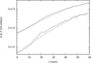
Figure 1: Modelling the dynamics of GDP (upper plot) and trade (lower plot) using World Bank data for USA (usg, ; ust, ). The dotted curves follow the logistic equation with the parameter values in Table 1. The zero year of both plots is 1960. The GDP plot ends in 2020, but the trade plot ends in 2019.

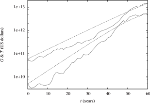
Figure 2: Modelling the dynamics of GDP (upper plot) and trade (lower plot) using World Bank data for China (cng, ; cnt, ). The dotted curves follow the logistic equation with the parameter values in Table 1. The zero year of both plots is 1960, and both end in 2020.

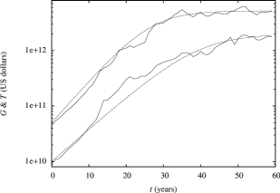
Figure 3: Modelling the dynamics of GDP (upper plot) and trade (lower plot) using World Bank data for Japan (jpg, ; jpt, ). The dotted curves follow the logistic equation with the parameter values in Table 1. The zero year of both plots is 1960, and both end in 2019.

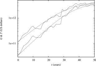
Figure 4: Modelling the dynamics of GDP (upper plot) and trade (lower plot) using World Bank data for Germany (deg, ; det, ). The dotted curves follow the logistic equation with the parameter values in Table 1. The zero year of both plots is 1970, and both end in 2020.

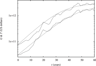
Figure 5: Modelling the dynamics of GDP (upper plot) and trade (lower plot) using World Bank data for UK (ukg, ; ukt, ). The dotted curves follow the logistic equation with the parameter values in Table 1. The zero year of both plots is 1960, and both end in 2020.

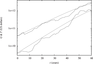
Figure 6: Modelling the dynamics of GDP (upper plot) and trade (lower plot) using World Bank data for India (ing, ; int, ). The dotted curves follow the logistic equation with the parameter values in Table 1. The zero year of both plots is 1960, and both end in 2020.

Table 1: Parameter values of the logistic equation for dynamically modelling the World Bank GDP data (usg, ; cng, ; jpg, ; deg, ; ukg, ; ing, ) and trade data (ust, ; cnt, ; jpt, ; det, ; ukt, ; int, ) of the six countries that are listed in the first column. The data have been plotted and modelled in Figs. 1 to 6. The last column lists the values of the power-law exponent in the correlated growth of GDP and trade, as plotted and modelled in Figs. 7 to 12.

	Parameters to fit $G$ (GDP)			Parameters to fit $T$ (Trade)
Country	$\gamma_{1}$ (per annum)	$k_{G}$ (trillion US dollars)	$t_{\mathrm{nl}}$ (years)	$\tau_{1}$ (per annum)	$k_{T}$ (trillion US dollars)	$t_{\mathrm{nl}}$ (years)	$G$-$T$ Correlation	$\alpha$
USA	$0.080$	$30.0$	$50$	$0.099$	$10.0$	$53$	$0.992$	$0.75$
China	$0.095$	$80.0$	$76$	$0.130$	$10.0$	$58$	$0.983$	$0.65$
Japan	$0.175$	$~{}~{}5.2$	$26$	$0.135$	$~{}~{}2.0$	$39$	$0.919$	$1.00$
Germany	$0.110$	$~{}~{}4.4$	$32$	$0.130$	$~{}~{}3.9$	$36$	$0.987$	$0.85$
UK	$0.105$	$~{}~{}3.0$	$35$	$0.095$	$~{}~{}2.5$	$46$	$0.993$	$0.90$
India	$0.080$	$~{}~{}6.0$	$64$	$0.100$	$~{}~{}3.0$	$66$	$0.982$	$0.60$

Table 2: Statistical analyses of the relative difference between the actual data and the model functions. The second column lists the mean $\mu_{G}$ and the standard deviation $\sigma_{G}$ of the yearly relative variations of the GDP data (usg, ; cng, ; jpg, ; deg, ; ukg, ; ing, ) with respect to the logistic model. Likewise, in the third column, $\mu_{T}$ and $\sigma_{T}$ are the mean and the standard deviation, respectively, of the yearly relative variations of the trade data (ust, ; cnt, ; jpt, ; det, ; ukt, ; int, ). The last column pertains to the $G$-$T$ correlation (as plotted in Figs. 7 to 12), with $\mu_{\alpha}$ and $\sigma_{\alpha}$ being, respectively, the mean and the standard deviation of the yearly relative variations of the logarithm of the GDP data (usg, ; cng, ; jpg, ; deg, ; ukg, ; ing, ), with respect to the logarithm of the model power-law function.

	Statistical analysis of $G(t)$ (GDP)		Statistical analysis of $T(t)$ (Trade)		Statistical analysis of $\alpha$
Country	$\mu_{G}$	$\sigma_{G}$	$\mu_{T}$	$\sigma_{T}$	$\mu_{\alpha}$	$\sigma_{\alpha}$
USA	$~{}~{}~{}0.0492$	$0.0873$	$~{}~{}~{}0.1160$	$0.2040$	$-0.0012$	$0.0024$
China	$-0.3568$	$0.2504$	$-0.3570$	$0.3393$	$~{}~{}~{}0.0075$	$0.0113$
Japan	$-0.0833$	$0.1395$	$~{}~{}~{}0.1900$	$0.3682$	$-0.0045$	$0.0082$
Germany	$~{}~{}~{}0.0489$	$0.1744$	$~{}~{}~{}0.0736$	$0.2411$	$-0.0034$	$0.0051$
UK	$-0.1089$	$0.1651$	$~{}~{}~{}0.0053$	$0.1679$	$-0.0019$	$0.0033$
India	$-0.1359$	$0.1743$	$-0.1630$	$0.3534$	$~{}~{}~{}0.0015$	$0.0079$

IV The dynamics of trade

The annual trade of a country accounts for the total import and export of goods and services. The World Bank data on annual trade are given as a percentage of the annual GDP of a country (ust, ; cnt, ; jpt, ; det, ; ukt, ; int, ). Knowing the annual GDP, the trade percentage can be expressed explicitly in terms of US dollars, which we denote by the variable $T\equiv T(t)$, with $t$ continuing to be measured in years. We model the dynamics of $T(t)$ with the logistic equation, as done in Eq. (4), and write

$$\dot{T}\equiv\frac{{\mathrm{d}}T}{{\mathrm{d}}t}={\mathcal{T}}(T)=\tau_{1}T-\tau_{2}T^{2}.$$ (5)

Comparing Eq. (5) with Eq. (1), we note that $x$, $a$ and $b$ translate, respectively, to $T$, $\tau_{1}$ and $\tau_{2}$. Hence, from the integral solution of $T(t)$, which will be in the same form as Eq. (2), we will get a convergence of $T\longrightarrow k_{T}=\tau_{1}/\tau_{2}$, when $t\longrightarrow\infty$.

The fitting of the integral solution of Eq. (5) with the trade data (ust, ; cnt, ; jpt, ; det, ; ukt, ; int, ) is shown in all the lower linear-log plots in Figs. 1 to 6. The values of $\tau_{1}$ (the relative annual growth rate of trade), $k_{T}$ (the predicted upper limit of trade) and $t_{\mathrm{nl}}$ (when nonlinearity sets in), using which we fit the model equation with the data, are given in Table 1. The consistency of the model fitting is statistically summarized in Table 2, which gives the mean $\mu_{T}$ and the standard deviation $\sigma_{T}$ of the yearly relative variations of the actual trade data (ust, ; cnt, ; jpt, ; det, ; ukt, ; int, ) with respect to the logistic function. In Figs. 1 to 6 we see that the model fitting for trade in the lower plots largely resembles the features of the model fitting for the GDP in the upper plots. This is very much true for USA, Japan, Germany and UK on the one hand and China on the other. In the case of India, the upper plot for GDP is more regular than the lower plot for trade, as can be seen in Fig. 6. The overall similarity between the two plots implies that there is a high correlation between the GDP and the trade of a country. Country-wise values of the GDP-trade correlation are in the second last column of Table 1. We look into this matter more closely in Sec. VI.

V Interpreting the logistic model

The irregularity of the two plots in Fig. 2 (and related values in Table 2) suggests that China is an anomalous case in modelling the dynamics of both GDP and trade with the logistic equation. The trade plot in Fig. 6 conveys a similar hint for India. These anomalies can be explained from the perspective of world history in the latter half of the twentieth century. In order to do so, we first consider all the three major economies of the North-Atlantic region and Japan in the Indo-Pacific. In the period that immediately followed the Second World War, which ended in 1945, USA was the only country among the principal belligerents of the war that possessed a fully operational industrial infrastructure. With the onset of the Cold War against the erstwhile Soviet Union, it became a policy imperative for USA to lend its industrial power for the economic revival of both Western Europe (under the Marshall Plan) and Japan. This resulted in a rapid re-industrialization of Japan and the erstwhile West Germany. Indeed, in the case of West Germany, the swiftness of the economic recovery from the ravages of the war is spoken of as the “German economic miracle.” In comparison, the post-war economic recovery of UK, which by then had also given up many of its bountiful colonies (most notably India), was slow. Nevertheless, by 1960, Japan, Germany and UK had achieved economic stability under the guidance of USA, in consequence of which these three countries were well set on the path of general prosperity. This comfortable state of affairs is reflected in the relatively ordered progression of the data (over several decades starting from 1960) and its close match with the model function in Figs. 3, 4 and 5 (with support from related values in Table 2).

In contrast, after the Second World War, the economic growth of China and a politically independent India did not experience the advantages that regenerated the economies of Japan, Germany and UK. For close to three decades after the Second World War, China continuously suffered from internal political upheavals like the Great Leap Forward and the Cultural Revolution. Unsurprisingly, therefore, during this period the economic growth of China was severely impeded. India, on the other hand, experienced domestic political stability in the same period, but its benefits were not visible on its post-colonial economic development, mainly due to government policies. What is more, both China and India were in a state of war several times (once between themselves) in the first two to three decades of their new beginning as sovereign states. The combined effect of all the adversities encountered by China and India can be observed in the irregular path traced by the GDP data in Fig. 2 and the trade data in Figs. 2 and 6.

In the light of the foregoing observations, we can now discern two distinct categories. In one category, the logistic equation fits the data in the expected manner. USA, Japan, Germany and UK belong to this category, with USA showing the greatest accuracy for the logistic fit, as in Fig. 1 and Table 2. We note certain characteristics that are common to these four countries. Since the end of the Second World War, all of them fostered universal democratic values in their internal politics, underwent no military conflict on their borders, and promoted free economic growth without much intervention from the state. The cumulative effect of these conditions is conducive to a natural development of material well-being. The absence of any one of the aforementioned conditions causes an imbalance and to a greater or lesser extent creates the second category. China and India are in the second category. Both countries have a record of conflict on their common border and borders with some of their other geographical neighbours. Both have government control in varying degrees on their respective economies. And specific to China, the political conditions within the country differ from the norms of democracy that prevail in the other five countries in this study. Under these circumstances, economic growth follows an uneven course, which, in the case of China, is marked by the discrepancy in the logistic modelling of the national economic data in both the plots in Fig. 2, and by having the highest absolute values of $\mu_{G}$ and $\mu_{T}$ among all the countries in Table 2. For India, the discrepancy is partial, as it is mostly seen in the trade plot in Fig. 6. This mitigation is due to the stable democratic polity in the country. Going by these observations, we contend that the balanced economic growth of a country (especially in terms of its GDP and trade data) can be gauged from the closeness of its match with the logistic equation (the closeness being quantified by small values of $\mu_{G}$, $\sigma_{G}$, $\mu_{T}$ and $\sigma_{T}$ in Table 2).

This raises a valid question about the general import of the logistic equation. It is known that the natural growth of many systems is described satisfactorily by the logistic equation, the growth of species being a standard example (Braun, 1983). Hence, the logistic equation is organically compatible with natural evolution in an open and productive environment. This principle arguably applies to the free evolution of economic systems as well, a point of view that is supported by Figs. 1, 3, 4 and 5.

VI The GDP-Trade correlation

At the end of Sec. IV, we mentioned the high correlation between the GDP and the trade of all the six countries in our study, something that is evident from the values of the $G$-$T$ correlation in the second last column of Table 1. This correlation is expected, because GDP and trade are dynamically connected to each other (Garlaschelli and Loffredo, 2004; Garlaschelli et al., 2007; Serrano, 2007). As such, the coupled dynamics of GDP and trade must be governed by an autonomous system of the second order, given as ${\dot{T}}={\mathcal{T}}(T,G)$ and ${\dot{G}}={\mathcal{G}}(T,G)$. The $T$-$G$ phase solutions are determined by integrating

$$\frac{{\mathrm{d}}G}{{\mathrm{d}}T}=\frac{\dot{G}}{\dot{T}}=\frac{{\mathcal{G}}(T,G)}{{\mathcal{T}}(T,G)}$$ (6)

for various initial values of the $(T,G)$ coordinates (Strogatz, 1994). Since the autonomous functions ${\mathcal{G}}(T,G)$ and ${\mathcal{T}}(T,G)$ are not known a priori, we proceed with a linear ansatz of ${\mathcal{G}}\simeq\gamma_{1}G$ from Eq. (4) and ${\mathcal{T}}\simeq\tau_{1}T$ from Eq. (5). This linearization is in accord with the multiplicative character of GDP and trade, whereby the revenue generated in one year is reinvested in the economic cycle of the next year (Garlaschelli et al., 2007). In the linear regime, we get a scaling formula that goes as (with $\alpha=\gamma_{1}/\tau_{1}$)

$$G(T)\sim T^{\alpha},$$ (7)

for which empirical evidence was found from 1948 to 2000, in a survey of nearly two dozen countries of varying economic strength (high, middle and low-income economies) (Bhattacharya et al., 2008).

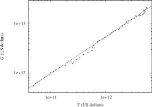
Figure 7: Plotting GDP against trade using World Bank data for USA (usg, ; ust, ). The dotted line follows Eq. (7) with $\alpha=0.75$ (see Table 1). The plot begins in 1960 and ends in 2019.

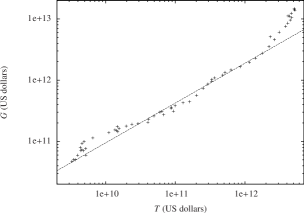
Figure 8: Plotting GDP against trade using World Bank data for China (cng, ; cnt, ). The dotted line follows Eq. (7) with $\alpha=0.65$ (see Table 1). The plot begins in 1960 and ends in 2020.

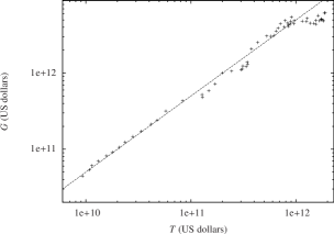
Figure 9: Plotting GDP against trade using World Bank data for Japan (jpg, ; jpt, ). The dotted line follows Eq. (7) with $\alpha=1.00$ (see Table 1). The plot begins in 1960 and ends in 2019.

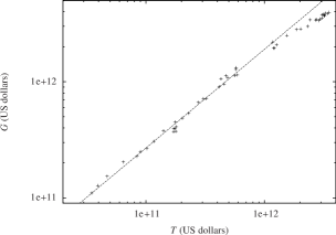
Figure 10: Plotting GDP against trade using World Bank data for Germany (deg, ; det, ). The dotted line follows Eq. (7) with $\alpha=0.85$ (see Table 1). The plot begins in 1970 and ends in 2020.

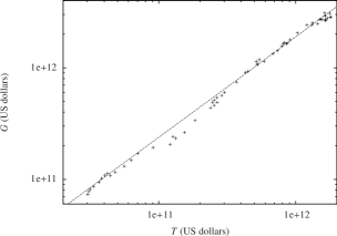
Figure 11: Plotting GDP against trade using World Bank data for UK (ukg, ; ukt, ). The dotted line follows Eq. (7) with $\alpha=0.90$ (see Table 1). The plot begins in 1960 and ends in 2020.

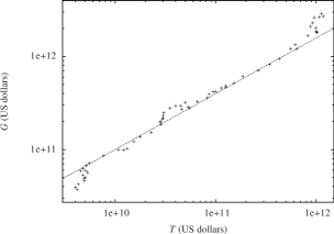
Figure 12: Plotting GDP against trade using World Bank data for India (ing, ; int, ). The dotted line follows Eq. (7) with $\alpha=0.60$ (see Table 1). The plot begins in 1960 and ends in 2020.

The power-law function in Eq. (7) becomes linear in a log-log plot. This is indeed what we see in Figs. 7 to 12, all of which model the coupled growth of GDP and trade up to 2020 (or 2019) for the six countries in our study. The power-law exponent $\alpha$, which is the slope of the linear fit, is confined within a narrow range of $0.6<\alpha<1$ in all cases. The country-wise values of $\alpha$ have been set down in the last column of Table 1. Keeping only the linear terms in Eqs. (4) and (5), which gives the phase solutions in Eq. (7), we find that $\alpha=\gamma_{1}/\tau_{1}$. The values of $\gamma_{1}$, $\tau_{1}$ and $\alpha$ in Table 1 do show that $\alpha$ is practically quite close to $\gamma_{1}/\tau_{1}$. This independently validates our modelling of GDP and trade growth with the logistic equation.

Looking at Figs. 7 to 12, we realize that the power-law scaling of $G$ with respect to $T$ holds true for every country over at least two orders of magnitude, an observation borne out consistently by the low values of $\mu_{\alpha}$ and $\sigma_{\alpha}$ in Table 2. For high values of $T$ and $G$, deviation from this scaling behaviour occurs for China, Japan, Germany and India (Figs. 8, 9 10 and 12, respectively). This deviation is due to the nonlinear effects in the real data, which we have not considered in the coupled autonomous functions ${\mathcal{G}}(T,G)$ and ${\mathcal{T}}(T,G)$, in deriving Eq. (7). We also note that ${\mathrm{d}}^{2}G/{\mathrm{d}}T^{2}<0$ for $\alpha<1$, i.e. $G$ increases with $T$ at a decreasing rate as time progresses. This explains the reduction of the gap between the GDP and the trade plots in Figs. 1 to 6 on long time scales.

The values of $\alpha$ in Table 1 hint at a possible distinction between two types of countries. In one type, which includes Japan, Germany and UK, $\alpha$ has a relatively high value. In the other type, which includes USA, China and India, $\alpha$ has a smaller value. The latter type of countries are geographically extended on continental or subcontinental scales, and have large populations. In contrast, countries of the former type are territorially restricted with comparatively small populations. This distinction between the two types of countries may cause qualitative differences in trading patterns (Frankel and Romer, 1999), with a concomitant effect on the GDP. We conjecture that the value of $\alpha$ segregates the two types of countries (about $\alpha=0.80$). More clarity on this point, however, requires a wider study.

VII Conclusions

Our study has brought two salient results to the fore. The first is that under conducive conditions, the logistic equation suffices to model the growth of GDP and trade. The conducive conditions refer to the state of internal politics, military engagements and economic policies of a country. The second result is a correlated growth of GDP and trade, driven by a power-law. The power law can be traced back to the logistic equation itself and the exponent of the power law possibly characterizes economies on the basis of geographical scales and population sizes. These theoretical claims are founded on empirical facts, and hold true across countries. Global validity can be attributed to these principles, even though our study covers six countries, because the country-wise distributions of GDP and trade have a scale-free order (Garlaschelli et al., 2007; Serrano and Boguñá, 2003; Garlaschelli and Loffredo, 2004).

A scale-free order, in which a small number of countries account for a large portion of the international trade (Bhattacharya et al., 2008), can be exploited to devise globally-coordinated strategies for the recovery of the world economy from the current Covid-19 pandemic. The first step in this respect is a vigorous re-activation of the international trade network. For this a leading role is essential from the two strategic economic regions that we have considered in our study, i.e. the North-Atlantic and the Indo-Pacific. Major shipping routes pass through both and many countries in or abutting the two oceanic regions have high national GDP. These countries form a regional trading cluster, in which their geographical proximity promotes trade (Tinbergen, 1962; Anderson, 2010; Benedictis and Taglioni, 2011). Once trade flourishes within an economic region, its main economic players can then trade with other economic regions, as it ought to be in the scale-free and small-world architecture of the global trade network (Serrano and Boguñá, 2003). Since GDP and trade are correlated, enhancement of trading activities will have a positive impact on the GDP of the participating countries.

Our theoretical modelling, based on the logistic equation, predicts long-term economic stagnation. Reasons for this are dwindling natural resources, natural calamities, pandemics, obsolescence of technology, military conflicts, etc. The decisive reasons are often unforeseen. Nevertheless, the logistic equation continues to be a favoured mathematical tool for modelling the evolution of socio-economic systems (Braun, 1983; Montroll, 1978). For example, our use of the logistic equation and the power-law correlation function in the phase plot was equally effective in modelling the growth of companies (Ray, 2010). This analogy between national economies and companies is of interest because studies point to universal mechanisms that underlie the economic dynamics of countries and companies (Stanley et al., 1996; Lee et al., 1998). This commonality can help in understanding the dynamics of large companies, whose stock values can grow to the scale of national economies. On this point, we note that major stock indices of the six countries in our study show as much regularity (Kakkad et al., 2020) as the GDP and trade growth of the same countries.