Prioritized Planning for Cooperative Range-Only Localization in Multi-Robot Networks

Abstract

We present a novel path-planning algorithm to reduce localization error for a network of robots cooperatively localizing via inter-robot range measurements. The quality of localization with range measurements depends on the configuration of the network, and poor configurations can cause substantial localization errors. To reduce the effect of network configuration on localization error for moving networks we consider various optimality measures of the Fisher information matrix (FIM), which have well-studied relationships with the localization error. In particular, we pose a trajectory planning problem with constraints on the FIM optimality measures. By constraining these optimality measures we can control the statistical properties of the localization error. To efficiently generate trajectories which satisfy these FIM constraints we present a prioritized planner which leverages graph-based planning and unique properties of the range-only FIM. We show results in simulated experiments that demonstrate the trajectories generated by our algorithm reduce worst-case localization error by up to 42% in comparison to existing planning approaches and can scalably plan distance-efficient trajectories in complicated environments for large numbers of robots.

I Introduction

Robotic systems have tremendous value in the advancement of scientific exploration, with robots collecting data on planetary surfaces [1], outer space [2], and in the deep oceans [3]. In these settings usage of multi-robot systems conveys several advantages: observations can be made more rapidly, over larger areas, and the robots can collaborate to more efficiently accomplish the mission. However, a key challenge in real-world deployment of mobile robotic systems in general is accurate localization.

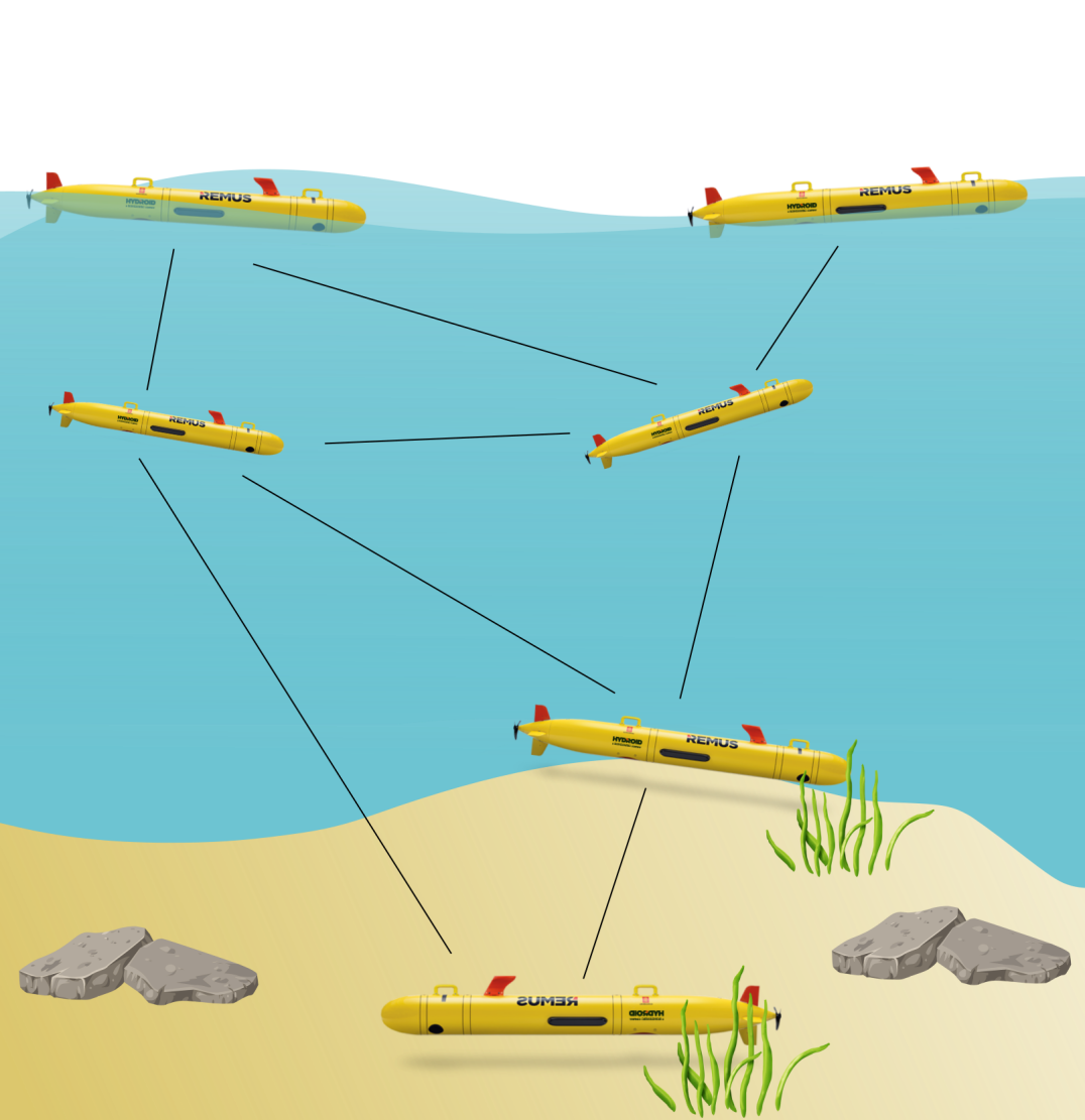
Figure 1: Network of robots performing cooperative localization via range measurements. Edges between robots indicate inter-robot range measurements. Robots on the surface are assumed to have ground-truth positioning via GNSS.

A common approach to multi-robot localization relies on teams in which the robots use inter-robot ranging and a subset of the robots are considered anchors [4, 5]. These anchors have high quality self-localization, possibly due to global navigation satellite systems (GNSS) or high-precision inertial systems, and enable for absolute localization of the remainder of the network through the relative range measurements. However, the accuracy of localizing the entire network via range measurements depends on the relative positioning of the agents [6] and the localization problem can become ill-posed under certain network configurations, causing localization techniques to fail drastically. As a result, as the team of robots moves throughout space the localization of the non-anchor robots can vary and substantially deteriorate. In safety-critical or high-cost missions poor localization can lead to disastrous outcomes such as loss of expensive equipment or even loss of life. To avoid the potential costs of poor localization we propose a technique for planning trajectories for such robot networks that effectively maintains a minimum localization quality at all timesteps.

We measure the ability for a given configuration to be localized through the Fisher information matrix (FIM) and FIM-based optimality measures from the field of design of experiments. These measures are scalar values that relate the FIM eigenvalues to various statistical properties of the localization problem [7]. By constraining these optimality measures with lower bounds, the localization quality of the network can be controlled. However, planning trajectories which constrain these measures is difficult, as the optimality measures are complicated functions of the network configuration which tightly couple the states of the separate robots in the network. The primary challenge is in the inherent dimensionality of the planning problem, as the individual robots cannot be easily decoupled and computational issues arise with the resulting complexity of the problem. We present a framework for decoupling the planning process and performing prioritized planning, i.e. planning each robot individually in a predetermined sequence, while ensuring that the network localization quality is maintained.

This paper extends our previous work on graph-based, prioritized, localizability-constrained planning [8] with the following contributions:

• The relationship between localization quality and the theory of design of experiments is made clear.

• We present original proofs relating network connectivity, the FIM, and FIM optimality measures.

• This paper considers the case where there are sufficient anchor robots to fully constrain the localization problem, whereas [8] neglected the effects of anchor robots.

• More extensive experimental results with a more computationally efficient localizability-constrained planner and greater accuracy localization approach.

• The source code will be made freely available

II Related Work

As our work seeks to control robot networks to improve their localization we first review similar works in the area of active localization. Then, as our described problem is in multi-robot planning, we review relevant works in the planning community. We note that our consideration of localization quality is closely related to the well-known geometric dilution of precision [9], but for brevity we do not discuss this in further depth.

II-A Active Localization

Prior works recognize the importance of geometry on the quality of range-only localization and consider how to control members of a team to improve the localization of others. Many approaches consider properties of either the FIM or the closely related covariance matrix as measures of localization quality [4, 10, 11]. Existing approaches learn a policy [12, 13] or perform belief space planning [10] for a single anchor vehicle to support a number of other vehicles. A different approach developed a distributed algorithm for any number of anchor vehicles to reduce the total uncertainty of any number of non-anchor vehicles [4]. However, these works assume that the non-anchor vehicles have fixed trajectories and do not consider how the non-anchor trajectories could be planned to improve their own localization.

Other works [11, 14] present potential-field methodologies for distributed trajectory planning for networks of anchor and non-anchor robots. In [11] potential functions are presented for several FIM optimality metrics. The work in [11] relates to earlier work in [14] which developed rigidity matrices to control the infinitesimal rigidity of such a network of robots, a necessary property for both control and localization in the range-only case. However, the approaches in [11, 14] are both potential-field based techniques. In these approaches, local minima in the potential fields trap the planner and prevent the network from reaching the goal locations. While our approach considers the same optimality measures as [11], our approach does not rely on the gradient of the optimality metrics and thus does not suffer from the very common local minima presented in these potential-field based approaches.

II-B Multi-Robot Planning

Each additional robot in the network increases the dimensionality of the planning problem. This leads to a challenge in the field of multi-robot planning known as the curse of dimensionality, which refers to how the size of the planning space scales exponentially with increasing dimensions. Prioritized planning, in which the robots in a network plan their trajectories independently in a predetermined sequence, has been proposed to reduce the effects of dimensionality [15]. In a similar vein, [16] presents the idea of subdimensional expansion. With this approach, trajectories are planned independently on a graph until interactions occur between robots, at which point the planner considers the joint configuration space of the interacting robots. Other works in multi-agent trajectory planning consider combinations of discrete and continuous representations of space [17, 18]. They also reduce the dimensionality by planning for subgroups of the robots at a time as opposed to the whole team at once, using different strategies to handle potential conflicts between robots. While these notions of dimensionality reduction are a key part of the approach we present, none of these approaches can be immediately extended to our problem as the FIM construction enforces that each robot needs to be considered as always interacting with all other robots.

III Problem Formulation

We begin by establishing the difference between anchor and non-anchor robots in our network. We present the FIM that will be referred to throughout this paper, as originally derived in [6], as well as the different optimality criteria of the FIM which our approach applies to. Finally, in this section, we formally define the problem this paper considers.

As in [6, 8], we assume that range measurements are either Gaussian or log-normally distributed. Additionally, we assume a sensing horizon which prevents robots from obtaining range measurements to each other if they are beyond a certain distance from each other.

III-A Terminology and Notation

Throughout this paper we use the abbreviation LC to refer to a localizability constraint (LC) and LC_SAT to refer to a set of positions that satisfy a group of localizability constraints, i.e the localizability constraint satisfying (LC_SAT) set. All indexing is zero-indexed, i.e. the first row in a matrix is the $0$th row. We use two separate neighbor functions: $\operatorname{\text{neigh}_{g}}(\cdot)$ acts on a set of nodes on a planning graph and returns the union of all neighboring locations of all locations in the set, $\operatorname{\text{neigh}}(\cdot)$ acts on a robot in a network and returns all of the robots it has range measurements to.

III-B Anchor and Non-Anchor Indexing

Anchor robots are robots which are considered to have known absolute position. In practice, this position information could be from sources such as GNSS or high-precision inertial navigation systems. We order the robots such that the anchors are grouped first and followed by the non-anchors, with no particular ordering within these subgroups. For example, if we have $\operatorname{n_{anc}}$ anchors and $\operatorname{n_{non}}$ non-anchors the indices are $\{0,\dots,\operatorname{n_{anc}},\dots,(\operatorname{n_{non}}+\operatorname{n_{anc}}-1)\}$.

III-C Fisher Information Matrix

We present the FIM in Equation 5 as derived in [6]. We begin by defining an undirected graph $\operatorname{{G}}=(\operatorname{{V}},\operatorname{{E}})$ over the network of robots where the edge $(i,j)$ exists if there is a range measurement between robots $i$ and $j$. The position of robot $i$ is denoted $x_{i}\in\mathbb{R}^{d}$. The FIM $F\in\mathbb{R}^{d\operatorname{n_{non}}\times d\operatorname{n_{non}}}$ is a ($d\times d$)-block-structured matrix which is similar to a weighted graph Laplacian over $\operatorname{{G}}$ where the Laplacian’s rows and columns corresponding to the indices of anchor nodes have been removed. The contributions of the sensor model in the FIM appear in the following parameters: $\gamma$, which is equal to 1 if the sensor model is Gaussian and 2 if the model is log-normally distributed, and $\sigma$, the standard deviation of the sensor distribution.

We first define the difference in robot positions and the distance between robots as follows:

$$\operatorname{\Delta_{\mathit{ij}}} \triangleq x_{i}-x_{j}\in\mathbb{R}^{d}$$ (1)

$$L \triangleq\|\operatorname{\Delta_{\mathit{ij}}}\|_{2}\in\mathbb{R}$$ (2)

From this, we define $b_{ij}\in\mathbb{R}^{d\operatorname{n_{non}}}$ and $q_{ij}\in\mathbb{R}^{d\operatorname{n_{non}}}$, which relate the relative positions of robots in the network to sub-blocks of the FIM. The vectors $b_{ij}$ and $q_{ij}$ are ($1\times d$)-block-structured vectors which relate nodes $i$ and $j$ whose $k$th-blocks are given in Equations 3 and 4.

$$b_{ijk} \triangleq\dfrac{\operatorname{\Delta_{\mathit{ij}}}}{\sigma L^{\gamma}}\begin{cases}1&k=i\\ -1&k=j\\ 0&\text{otherwise}\end{cases}$$ (3)

$$q_{ijk} \triangleq\dfrac{\operatorname{\Delta_{\mathit{ij}}}}{\sigma L^{\gamma}}\begin{cases}1&k=i\\ 0&\text{otherwise}\end{cases}$$ (4)

We next define $\operatorname{{E}_{na}}$ as the set of edges between a non-anchor node and an anchor node and $\operatorname{{E}_{nn}}$ as the set of edges between two non-anchor nodes. In the case of $\operatorname{{E}_{na}}$ we assume without loss of generality that for each edge-pair $(i,j)\in\operatorname{{E}_{na}}$ the first value, $i$, refers to the non-anchor node. With these edge sets the FIM, $F\in\mathbb{R}^{d\operatorname{n_{non}}\times d\operatorname{n_{non}}}$, can be expressed as follows:

$$F=\sum_{(i,j)\in\operatorname{{E}_{na}}}b_{ij}b_{ij}^{\top}+\sum_{(i,j)\in\operatorname{{E}_{nn}}}q_{ij}q_{ij}^{\top}$$ (5)

Note that there is no contribution from edges between two anchor nodes, as the positions are known and thus no information is gained from such measurements.

As shown in [11, 14], the eigenvalues of the FIM are invariant to rigid-motion transformations of the network members and the FIM is similar to a weighted Laplacian of the connectivity graph of the network. Unsurprisingly, the weights in the Laplacian representation come exactly from the sensor measurement model and the relative positioning of the robots with respect to each other. By construction the FIM is a real, symmetric, positive semidefinite matrix, meaning all eigenvalues are nonnegative.

III-D Localizability Criteria

In design of experiments there are several common optimality measures which relate the eigenvalues of the FIM to quality of the underlying estimation [7]. For our problem this can be thought of as different measures of how the network configuration at a given timestep affects the underlying information geometry and, as a result, the localization quality.

As our approach uses prioritized planning, these measures are observed with increasing numbers of robots in the network, which corresponds to inference problems of increasing dimensionality. Because of this changing dimensionality, it can be difficult to relate the values of these optimality measures as robots are added to the network. For this reason, we focus on A-optimality and E-optimality in this paper, as they are relatively consistent as robots are added, and do not consider other popular measures such as D-optimality, which measures the volume of the covariance ellipsoid and thus grows geometrically with increasing robots.

We present A- and E-optimality in Equations 6 and 7 and refer the interested reader to [7] for theoretical properties of these measures as well as a list of other possible measures. We define $\operatorname{\mathbf{p}}\in\mathbb{R}^{dn}$ as the vector of robot positions for $n$ robots in the network and $F(\operatorname{\mathbf{p}})$ as the FIM that is formed from that configuration of robots. The optimality measures are then as follows:

$$\operatorname*{argmax}_{p}~{}\operatorname*{-\text{Tr}[F(\operatorname{\mathbf{p}})^{-1}]} (\text{A-optimal design})$$ (6)

$$\operatorname*{argmax}_{p}~{}\operatorname*{\lambda_{\min}(F(\operatorname{\mathbf{p}}))} (\text{E-optimal design})$$ (7)

We consider LCs to be predetermined, user-specified minimum values on these measures. Under the LCs defined by Equations 6 and 7 the set of allowed locations is $\bf{p_{all}}=\{\operatorname{\mathbf{p}}\in\mathbb{R}^{dn}:\operatorname{\operatorname*{-\text{Tr}[F(\operatorname{\mathbf{p}})^{-1}]}\geq\alpha;\operatorname*{\lambda_{\min}(F(\operatorname{\mathbf{p}}))}\geq\beta}\}$ for some user-defined values of $\alpha$ and $\beta$. For a general set of such user-defined criteria, we refer to network configurations which satisfy those criteria as localizability-constrained.

III-E Planning Problem Definition

Given the ability to compute the FIM for a given network, we describe our localizability constrained planning problem. This problem takes as input a set of beginning locations ($\operatorname{\mathbf{p}}(0)$), a set of goal locations ($\operatorname{\mathbf{p}}(t_{f})$), and a set of LCs $\{\operatorname{\operatorname*{-\text{Tr}[F(\operatorname{\mathbf{p}})^{-1}]}\geq\alpha;\operatorname*{\lambda_{\min}(F(\operatorname{\mathbf{p}}))}\geq\beta}\}$. Given these inputs, the problem is to find trajectories for each robot ($\operatorname{\mathbf{p}}_{i}(t)$) such that each robot begins at its starting position, ends at its goal position, and the LCs of the network are satisfied at every timestep.

IV Localizability Constrained Planning

To solve the planning problem described in Section  III-E we present a prioritized, graph-based planner which plans for all robots on a single, common graph. To allow for scalability to larger numbers of robots we use a prioritized approach [15] to reduce the computational cost of planning from the $dn$-dimensional joint-configuration space of the robot network to the cost of planning in the $d$-dimensional configuration space of just a single robot. The graph-based planning is a probabilistic roadmap [19] approach in which we consider the network to move along the graph in discrete timesteps and enforce LCs at each timestep. We make use of constraint sets from our previous work [8] to efficiently enforce the LCs. In particular, we require that the trajectories planned for each robot $i$ stay within what we term the valid set, $\operatorname{\mathbf{V}}_{i,t}$ in Equation 15, for all timesteps $t$.

IV-A Constraint Sets

The trajectory of the robot network can be thought of as a time-indexed sequence of networks, with each network corresponding to a unique timestep. Similarly, prioritized planning for each robot can be thought of as adding a single node to each timestep-indexed network. This framework for viewing the problem is key in understanding the benefit of the constraint sets described in this section, as the constraint sets represent where nodes can be added to maintain certain constraints on the network.

We plan each robot’s trajectory separately and the localization conditions for each timestep are independent of each other. For each robot $i$ and timestep $t$, there is a separate set of constraint sets $\{\operatorname{\mathbf{P}}_{i,t},\operatorname{\mathbf{C}}_{i,t},\operatorname{\mathbf{L}}_{i,t},\operatorname{\mathbf{V}}_{i,t}\}$. Constraint sets were first described in our previous work [8] as a means to reduce the necessary computation to perform planning. The constraint sets presented in this paper are the same concept as those from our previous work, with the notable difference in that we replace the rigid set, $\operatorname{\mathbf{R}}_{i,t}$ in [8], with the localizability constraint satisfying LC_SAT set, $\operatorname{\mathbf{L}}_{i,t}$. In [8] $\operatorname{\mathbf{R}}_{i,t}$ was constraining the E-optimality of the network, albeit without directly stating this relationship, whereas $\operatorname{\mathbf{L}}_{i,t}$ allows for a combination of such optimality constraints and more directly ties into the theory of design of experiments.

Effectively, we use relationships between the constraint sets to reduce the actual search space for each robot to a small subset of the actual nodes in the planning graph. In this approach, the search space is reduced to what we term the valid set, $\operatorname{\mathbf{V}}_{i,t}$, which, for non-anchor robots is the intersection of all other constraint sets corresponding to robot $i$ at timestep $t$.

We begin by defining the boolean indicator function for the LC_SAT set in Equation 11. We slightly abuse notation in using $\operatorname{\mathbf{x}}$ to indicate the position of an arbitrary node in the planning graph, whereas $\mathbf{x}_{k,t}$ refers to the position of robot $k$ at timestep $t$ according to a planned trajectory. The indicator function, $\operatorname{\operatorname{\mathbb{I}}_{L\operatorname{\text{-}}C}}(\mathbf{x},i,t)$, evaluates to true if and only if at timestep $t$ the set of network positions formed by the position $\operatorname{\mathbf{x}}$ in addition to the positions of all previously planned robots $(0,\dots,i-1)$ satisfies the user-determined localizability criteria.

We formally define $\operatorname{\mathbf{p_{x,t}}}$ in Equation 8, where $\{\mathbf{x}_{0,t},\mathbf{x}_{1,t},\dots,\mathbf{x}_{i-1,t}\}$ is a partial assignment of robot positions from the robots before $i$ in the priority queue. This arises from the prioritized planning, as the trajectories for robots $0$ to $i-1$ will have been planned, so the positions of all of these robots at a given timestep will be fixed. As such, $\operatorname{\mathbf{p_{x,t}}}$ suggests that the set of positions considered is just indexed by an arbitrary position $x$ as all other positions in the set are fixed given the timestep $t$.

$$\operatorname{\mathbf{p_{x,t}}} \triangleq\{\operatorname{\mathbf{x}}\}\cup\{\mathbf{x_{0,t}},\mathbf{x_{1,t}},\dots,\mathbf{x_{i-1,t}}\}$$ (8)

$$\operatorname{\mathbf{A}} \triangleq(\operatorname*{-\text{Tr}[F(\operatorname{\mathbf{p_{x,t}}})^{-1}]}\geq\alpha)$$ (9)

$$\operatorname{\mathbf{E}} \triangleq(\operatorname*{\lambda_{\min}(F(\operatorname{\mathbf{p_{x,t}}}))}\geq\beta)$$ (10)

$$\operatorname{\operatorname{\mathbb{I}}_{L\operatorname{\text{-}}C}}(\mathbf{x},i,t)\triangleq\operatorname{\mathbf{A}}\land\operatorname{\mathbf{E}}$$ (11)

The constraint sets are defined as follows, where $i$ and $j$ index robots, $t$ indexes timesteps, and $\rho$ is the radius of the sensing horizon:

$$\operatorname{\mathbf{P}}_{i,t}=\operatorname{\mathbf{V}}_{i,t-1}\cup~{}\operatorname{\text{neigh}_{g}}(\operatorname{\mathbf{V}}_{i,t-1}) (\text{Reachable Set})$$ (12)

$$\operatorname{\mathbf{C}}_{i,t}=\bigcup_{j=1}^{i-1}\{\operatorname{\mathbf{x}}:\|\operatorname{\mathbf{x}}-\mathbf{x}_{j,t}\|_{2}\leq\rho\} (\text{Connected Set})$$ (13)

$$\operatorname{\mathbf{L}}_{i,t}=\{\operatorname{\mathbf{x}}:\operatorname{\operatorname{\mathbb{I}}_{L\operatorname{\text{-}}C}}(\mathbf{x},i,t)\} (\text{LC\textsubscript{SAT} Set})$$ (14)

$$\operatorname{\mathbf{V}}_{i,t}=\begin{cases}\operatorname{\mathbf{P}}_{i,t}&i\leq\operatorname{n_{anc}}\\ \operatorname{\mathbf{P}}_{i,t}\cap\operatorname{\mathbf{L}}_{i,t}&i>\operatorname{n_{anc}}\\ \end{cases} (\text{Valid Set})$$ (15)

The reachable set $\operatorname{\mathbf{P}}_{i,t}$ represents all points that robot $i$ can get to by timestep $t$ while remaining within the valid set at all previous timesteps. The connected set $\operatorname{\mathbf{C}}_{i,t}$ represents all points that robot $i$ can occupy at timestep $t$ while being within the sensing horizon of one of the positions of the already planned robots ($\mathbf{x}_{0,t},\ldots,\mathbf{x}_{i-1,t}$) at that timestep. The localizability-constrained set $\operatorname{\mathbf{L}}_{i,t}$ is the set of all positions which satisfy the described localizability indicator function, defined in Equation 11. Finally, the valid set $\operatorname{\mathbf{V}}_{i,t}$ is the true set of interest in that it describes locations which robot $i$ can reach by time $t$ while satisfying the LCs at all times.

Within this work we assume the existence of $d+1$ anchor robots, which have known position and therefore for these robots if a location is reachable we consider it valid, whereas for the non-anchor robots a location must satisfy LCs as well as be reachable to be valid. In fact, as we assume the existence of three anchors, we prove in Lemma 1 and Theorem 2 that if at least one non-anchor robot has fewer than $d$ range measurements to it the FIM must be singular.

Lemma 1 ($d$-Connectivity and FIM Singularity)

Given the FIM defined in Equation 5, for any number of non-anchor nodes, if there exists a non-anchor node with less than $d$ neighbors the FIM will be singular.

Theorem 2 (Localizability Requires $d$-Connectivity)

Consider the localizability constraint indicator $\operatorname{\operatorname{\mathbb{I}}_{L\operatorname{\text{-}}C}}$ as in Equation 11. We define a nontrivial constraint to be an assignment of $\{(\alpha,\beta):(\alpha>-\infty)\lor(\beta>0)\}$. Given nontrivial constraints, if there exists $\operatorname{\mathbf{x}}_{i}\in\operatorname{\mathbf{p_{x,t}}}$ such that $(|\operatorname{\text{neigh}}(\operatorname{\mathbf{x}}_{i})|<d)$ then the localizability constraints must be violated, i.e. $\operatorname{\operatorname{\mathbb{I}}_{L\operatorname{\text{-}}C}}$ must evaluate to false.

This relationship between the FIM and the connectivity of the non-anchor robots leads to the result that for any reasonable LCs using any of the criteria in Equations 6 to 7 the relationship in Equation 16 holds.

$$\operatorname{\mathbf{L}}_{i,t}\subseteq\operatorname{\mathbf{C}}_{i,t}$$ (16)

We take advantage of the relationship in Equation 16 when constructing the constraint sets, as in general checking whether a given position is in the LC_SAT set ($\operatorname{\mathbf{x}}\in\operatorname{\mathbf{L}}_{i,t}$) requires computing the eigenvalues of the FIM. As the FIM, and thus its eigenvalues, differ for every possible $\operatorname{\mathbf{x}}$, constructing the FIM and finding eigenvalues becomes computationally demanding. To reduce the necessary computation, we only check states which are already connected, i.e. $\operatorname{\mathbf{x}}\in\operatorname{\mathbf{C}}_{i,t}$.

Algorithm 1 Localizability-constrained priority planning over a shared graph for network of robots

1:procedure Multi-Robot Planning

2:     $\text{trajectories}\leftarrow\emptyset$

3:     $\operatorname{\mathbf{V}}_{0}\leftarrow\text{Construct Valid Sets (0)}$

4:     $i\leftarrow-\operatorname{n_{anc}}$ $\triangleright$ robot index

5:     $n\leftarrow$ size of network

6:     while $i<\operatorname{n_{non}}$ do

7:         $\text{traj}\leftarrow\text{Perform Planning}(\operatorname{\mathbf{V}}_{i},i)$

8:         $\text{trajectories}_{i}\leftarrow\text{traj}$

9:         $\operatorname{\mathbf{V}}_{i}=\text{Construct Valid Sets}(i)$

10:         if $\operatorname{\mathbf{V}}_{i}=\emptyset$ then

11:              return $\emptyset$ $\triangleright$ planning failed          

12:         $i\leftarrow(i+1)$      

13:     return trajectories $\triangleright$ planning successful

Algorithm 2 Construct valid sets for robot $i$ at all timesteps from the trajectories of the previous robots

1:function Construct Valid Sets($i$)

2:     $P_{i,0}\leftarrow$ robot $i$ start location

3:     $V_{i,0}\leftarrow P_{i,0}$

4:     $t\leftarrow 0$

5:     $x\leftarrow$ goal location of robot $i$

6:     while $x\not\in\operatorname{\mathbf{V}}_{i,t}$ do

7:         $N\leftarrow$ all neighbors of $\operatorname{\mathbf{V}}_{i,t}$

8:         $\operatorname{\mathbf{P}}_{i,t+1}\leftarrow(\operatorname{\mathbf{V}}_{i,t}~{}\cup~{}N)$

9:         if $i\leq 2$ then

10:              $\operatorname{\mathbf{V}}_{i,t+1}\leftarrow\operatorname{\mathbf{P}}_{i,t+1}$

11:         else

12:              $\operatorname{\mathbf{L}}_{i,t+1}^{cand}\leftarrow\operatorname{\mathbf{P}}_{i,t+1}\cap\operatorname{\mathbf{C}}_{i,t+1}$

13:              $\operatorname{\mathbf{V}}_{i,t+1}\leftarrow\text{Get LC\textsubscript{SAT} States}(\operatorname{\mathbf{L}}_{i,t+1}^{cand},i,t+1)$          

14:         $t\leftarrow t+1$      

15:     return $V_{i}$ {Returning valid sets}

Furthermore, notice that the only set needed to perform planning is the valid set, and as valid states must be reachable (from Equation 15) we can improve efficiency by only checking the LC_SAT conditions for states which are also reachable, i.e. $\operatorname{\mathbf{x}}\in(\operatorname{\mathbf{C}}_{i,t}\cap\operatorname{\mathbf{P}}_{i,t})$. This is seen in 12 and 13 of Algorithm 2, where the intersection of the reachable and connected sets form the candidate states for the valid set.

IV-B Prioritized Planning

Given a planning graph, the prioritized planning proceeds by iterating over all the robots in the network in the predetermined order, first generating the constraint sets for that robot and then performing planning along the graph such that the robot $i$ is within the valid set $\operatorname{\mathbf{V}}_{i,t}$ for all timesteps $t$. This process is repeated for each robot in sequence until either all robot trajectories have been planned or the planner has failed. The planner is considered to fail if in the constraint set construction phase the valid sets never contain the goal location for that robot. As after a given amount of timesteps the valid sets will either become empty or reach a steady-state and no longer include new positions, it is simple in practice to check if the planner fails in this manner. If at some point the valid set $\operatorname{\mathbf{V}}_{i,t}$ possesses the goal location for robot $i$ then it is guaranteed by the definition of the valid set that there exists a trajectory to that robot’s goal position which satisfies the LC_SAT conditions at all timesteps. In this event, set construction is considered successful.

In our previous work [8] we presented a conflict-based approach for attempting to handle failures in the constraint set construction phase. However, in practice we observed no occasions where the conflict resolution approach led to successful replanning within any reasonable timespan. For this reason we remove this aspect from the planning framework described here in favor of an approach which fails outright when a trajectory cannot be found. As the success of prioritized planning can depend on the planning order, planning failures can be followed by a reordering and subsequent replanning attempts.

As the anchor robots are necessary in evaluating the LCs, the anchor robots are assumed to be planned before the non-anchor robots. Beyond this, no requirements are made on the ordering of the planning, the method to generate the planning graph, or the graph-based planner used.

V Results

TABLE I: Information and results from experiments. Each test case represents a unique set of obstacles, goal locations, and number of robots in the network. The three environments we tested in have no obstacles, two small obstacles, and two large obstacles, which we have categorized as low, medium, and high environmental complexity. We present the planning time required, number of ordering attempts required to successfully generate a plan for (Orderings), the maximum and average localization errors (MLE and ALE, respectively), and the average distance a robot moved from the start to goal (AD).
*The average and max error for the RRT approach for test case 2 are not included since one robot moved out of the sensing range of all other robots, which prevented the solver from producing a solution for the network during those timesteps.

Test Case	# Robots	Env. Complexity	Algorithm	Planning Time (s)	Orderings	ALE (m)	MLE (m)	AD (m)
1	6	Low	LCGP (Ours)	2.908	1	0.063	0.129	36.272
			RRT	0.381	–	0.050	0.132	42.257
			A*	2.979	–	0.076	0.212	36.02
			Potential Field	0.160	–	0.049	0.087	34.641
2	8	Medium	LCGP (Ours)	6.148	7	0.094	0.199	45.41
			RRT	2.657	–	*	*	60.00
			A*	3.968	–	0.103	0.213	45.00
			Potential Field	–	–	–	–	–
3	8	High	LCGP (Ours)	4.980	1	0.089	0.516	83.74
			RRT	8.614	–	0.095	0.889	108.69
			A*	5.017	–	0.171	0.705	80.64
			Potential Field	–	–	–	–	–
4	12	High	LCGP (Ours)	7.711	1	0.073	0.217	83.55
			RRT	13.846	–	0.091	0.377	111.54
			A*	7.930	–	0.069	0.225	83.50
			Potential Field	–	–	–	–	–
5	20	High	LCGP (Ours)	20.902	7	0.049	0.119	78.38
			RRT	20.147	–	0.050	0.136	100.20
			A*	16.625	–	0.048	0.100	77.89
			Potential Field	–	–	–	–	–

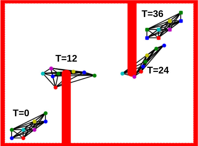
Figure 2: Snapshots of planned trajectory in example environment (Test Case 2). Dots indicate robots and lines indicate range measurements between robots. The configurations at timestep 0 and 36 are the start and goal. The network is qualitatively observed to maintain a triangulated configuration.

We tested our localization-constrained graph planning (LCGP) framework over a number of two-dimensional simulated environments with varying numbers of robots and obstacles. One of the tested environments and corresponding trajectories in mid-execution is shown in Figure 2 for reference. We set the first three robots as anchors (having known position) and the remaining robots as non-anchors (having unknown positions).

We compare statistics on timing, planning, and localization for our planning technique to three alternatives. We test against a prioritized RRT planner [20], against a prioritized A* planner, and against the potential field motion planner of [11] with E-optimality terms. All planners were implemented in Python and run on an Intel i7-10875H processor.

To generate our planning graph, we use a Halton sequence to sample the environment. Edges were made between every sampled node and neighbors within 2 units, excluding edges that intersect obstacles. We assume each robot to be a point robot and that there are no kinematic restrictions on a robot’s movement. To then perform planning on this graph, we use heuristic-directed A* search with the Euclidean distance from a node to the goal location as the heuristic.

Ordering is known to have substantial effects on the results of prioritized planning. In the event of a failed planning, the planning order of the non-anchor robots was reshuffled and planning was reattempted. In cases 2 and 5, the initial ordering did not produce a viable trajectory, so an alternative ordering was attempted.

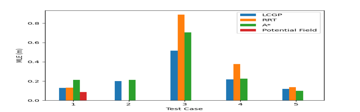
Figure 3: Max localization errors across all test cases.

During planning we constrained E-optimality to be greater than a value of 0.1 and placed no constraints on the A-optimality. This was justified by tests we ran, which compared localization quality to various combinations of A-optimality and E-optimality constraints and indicated that A-optimality measures had relatively little effect on localization error in comparison to E-optimality.

V-A Localization

To compare the ability to localize over the course of a given path, we implemented a nonlinear least-squares solver to find the maximum a posteriori estimate and report both the mean error across all non-anchor robots at all timesteps in the network and the max error of the mean across all non-anchor robots at a single timestep. This error is calculated as the Euclidean distance between the localization estimates and the ground truth positions.

The results for trajectories generated by our algorithm show the least max localization errors in all instances except for the potential field in case 1 and A* in test case 5. The greatest improvement was in test case 3, where LCGP reduced the maximum localization error 42% as compared to RRT and 26% relative to A*. The average localization errors for our algorithm are also comparable or lower than the alternatives for all cases. These results indicate that localizability-constrained planning constructs trajectories which improve range-only localization.

V-B Planning

To evaluate the feasibility of each planner, we report the time required to plan and the average distance travelled for each robot. In the case of LCGP, the planning time includes the time required to build the planning graph and replan using alternate orderings if necessary.

In environments with marked complexity or more challenging obstacles, notably cases 3, 4, and 5, we found that our approach was as fast as or faster than the RRT approach if the initial ordering succeeded. In test cases with any obstacles (2-5), the potential field approach failed to find a trajectory to the goal configuration due to local minima. The relative speed of our LCGP planner as compared to the RRT planner increased as either the number of robots or the complexity of the environment increased. However, in more simple environments with a large amount of free space, the RRT planner was able to plan trajectories up to an order of magnitude faster than the LCGP approach, as seen in cases 1 and 2.

Beyond planning time, we note that our LCGP approach found trajectories with notably shorter execution distances compared to our RRT implementation. This difference between our RRT implementation and our LCGP algorithm is likely due to the use of A* to perform planning on the graph, which encourages the LCGP planner to minimize travel distance. In comparison, the RRT approach would often generate inefficient trajectories with no weight given to the travel time. We do not compare the resulting distances to the theoretically optimal distances, but these results along with qualitative inspection of the trajectories indicate that the LCGP planner does generate distance-efficient trajectories.

VI Conclusions

In this paper we present a framework for efficiently planning localizability-constrained trajectories for a network of robots localizing via inter-robot ranging. We relate localization constraints to design of experiments and prove that for $d$-dimensional localization every robot of unknown position must have range measurements to at least $d$ other robots in the network to satisfy our localization constraints. We validate the effectiveness of our planning approach and its effect on the localization errors through extensive simulations.

Continuation of this work could consider the effects of different localizability measures on the localization error. Additionally, future work could explore how existing approaches in optimization-based trajectory planning can be modified to accommodate localization constraints.

VII Appendix

VII-A Proof of Lemma 1

To show that in a network where any non-anchor node has fewer than $d$ neighbors the FIM is singular, we first demonstrate that the FIM has at least $d$ zero-eigenvalues when a non-anchor node has no neighbors and then demonstrate that $d$ neighbors are the minimum number required to eliminate all of the zero-eigenvalues. Our proof focuses on the column structure of the FIM, but the FIM is symmetric, so the same arguments apply to the row-structure of the FIM.

Recall that the FIM $F\in\mathbb{R}^{dn\times dn}$ is a ($d\times d$)-block-structured matrix, with the $i$th ($dn\times d$) block-column relating to position of non-anchor robot $i$. From Equation 5 it is apparent that the FIM is the sum of rank-1 updates from the vectors $b_{ij}$ and $q_{ij}$ corresponding to measurements in the network. It directly follows from Equations 3 and 4 that if non-anchor node $i$ has no neighbors then the $i$th block-column will be entirely zeros. By the size of the block-column, the FIM must then have at least $d$ columns of zero-vectors and therefore have at least $d$ zero eigenvalues.

By continuation of this idea, in the previous case the $d$ eigenvectors corresponding to the zero eigenvalues are known to correspond to the $d$ dimensions in robot $i$’s position. The FIM is a series of rank-1 updates where the dimensions affected by the updates are in the direction of the vectors $b_{ij}$ and $q_{ij}$. Similarly, from Equations 3 and 4 it follows that the direction of the update only affects the dimensions corresponding to robot $i$’s position if the update corresponds to a measurement edge including robot $i$.

As each rank-1 update can only affect a single direction in the $d$-dimensional null-space, there must be $d$ linearly independent rank-1 updates to make the FIM non-singular. To have $d$ linearly independent rank-1 updates requires at least $d$ measurement edges involving robot $i$. Therefore if robot $i$ has less than $d$ neighbors the FIM is singular. ∎

VII-B Proof of Theorem 2

For an arbitrary nontrivial constraint defined by $(\alpha,\beta)$ as in Theorem 2 and its corresponding constraint indicator function $\operatorname{\operatorname{\mathbb{I}}_{L\operatorname{\text{-}}C}}$. We show that in the event that any non-anchor node has less than $d$ neighbors in the network any nontrivial constraint will be violated. By Lemma 1, if a non-anchor node has less than $d$ neighbors the FIM will be singular. If the FIM is singular it immediately follows that $\operatorname*{\lambda_{\min}(F(\operatorname{\mathbf{p}}))}=0$ and thus any nontrivial E-optimality constraint is violated. Similarly, as the FIM approaches a singular representation the A-optimality metric approaches negative infinity, i.e. $\lim_{\lambda_{min}\to 0}~{}\operatorname*{-\text{Tr}[F(\operatorname{\mathbf{p}})^{-1}]}\to-\infty$, and thus in the limit violates any nontrivial A-optimality constraint. As $\operatorname*{-\text{Tr}[F(\operatorname{\mathbf{p}})^{-1}]}$ is undefined when the FIM is singular as the FIM cannot be inverted, we consider the limiting behavior to show violation of nontrivial A-optimality constraints. Thus if any non-anchor node has less than $d$ neighbors any nontrivial constraint set will be violated. ∎

References

- [1] Tara A. Estlin et al. “AEGIS Automated Science Targeting for the MER Opportunity Rover” In ACM Transactions on Intelligent Systems and Technology 3.3, 2012 DOI: 10.1145/2168752.2168764
- [2] Yang Gao and Steve Chien “Review on space robotics: Toward top-level science through space exploration” In Science Robotics 2.7, 2017 DOI: 10.1126/scirobotics.aan5074
- [3] Yanwu Zhang et al. “A system of coordinated autonomous robots for Lagrangian studies of microbes in the oceanic deep chlorophyll maximum” In Science Robotics 6.50, 2021, pp. 1–12 DOI: 10.1126/SCIROBOTICS.ABB9138
- [4] A. Bahr, J.J. Leonard and A. Martinoli “Dynamic Positioning of Beacon Vehicles for Coop- erative Underwater Navigation” In IEEE/RSJ Intl. Conf. on Intelligent Robots and Systems (IROS), 2012
- [5] A. Bahr and J.. Leonard “Minimizing Trilateration Errors in the Presence of Noisy Landmarks” In European Conference on Mobile Robots, 2007
- [6] Neal Patwari et al. “Relative location estimation in wireless sensor networks” In IEEE Transactions on signal processing 51.8 IEEE, 2003, pp. 2137–2148
- [7] Friedrich Pukelsheim “Optimal design of experiments” SIAM, 2006
- [8] Alan Papalia and John Leonard “Network Localization Based Planning for Autonomous Underwater Vehicles with Inter-Vehicle Ranging” In IEEE/OES Autonomous Underwater Vehicles Symposium, 2020 IEEE
- [9] Richard B Langley “Dilution of Precision” In GPS world 10.5, 1999, pp. 52–59
- [10] Jeffrey M. Walls, Stephen M. Chaves, Enric Galceran and Ryan M. Eustice “Belief Space Planning for Underwater Cooperative Localization” In IEEE/RSJ Intl. Conf. on Intelligent Robots and Systems (IROS) 2015-Decem, 2015, pp. 2264–2271 DOI: 10.1109/IROS.2015.7353681
- [11] Jerome Le Ny and Simon Chauvière “Localizability-Constrained Deployment of Mobile Robotic Networks with Noisy Range Measurements” In Proceedings of the American Control Conference 2018-June AACC, 2018, pp. 2788–2793 DOI: 10.23919/ACC.2018.8431528
- [12] Mandar Chitre “Path Planning for Cooperative Underwater Range-Only Navigation using a Single Beacon” In Intl. Conf. on Autonomous and Intelligent Systems IEEE, 2010 DOI: 10.1109/AIS.2010.5547044
- [13] Yew Teck Tan, Rui Gao and Mandar Chitre “Cooperative path planning for range-only localization using a single moving beacon” In Journal of Oceanic Engineering 39.2 IEEE, 2014, pp. 371–385 DOI: 10.1109/JOE.2013.2296361
- [14] Daniel Zelazo, Antonio Franchi, Heinrich H. Bülthoff and Paolo Robuffo Giordano “Decentralized rigidity maintenance control with range measurements for multi-robot systems” In International Journal of Robotics Research 34.1, 2015, pp. 105–128 DOI: 10.1177/0278364914546173
- [15] Jur P. Van Den Berg and Mark H. Overmars “Prioritized Motion Planning for Multiple Robots” In IEEE/RSJ Intl. Conf. on Intelligent Robots and Systems (IROS), 2005, pp. 2217–2222 DOI: 10.1109/IROS.2005.1545306
- [16] Glenn Wagner and Howie Choset “M*: A Complete Multirobot Path Planning Algorithm with Optimality Bounds” In IEEE/RSJ Intl. Conf. on Intelligent Robots and Systems (IROS), 2011, pp. 3260–3267 DOI: 10.1007/978-3-642-33971-4_10
- [17] Jungwon Park, Junha Kim, Inkyu Jang and H. Kim “Efficient Multi-Agent Trajectory Planning with Feasibility Guarantee using Relative Bernstein Polynomial” In IEEE Intl. Conf. on Robotics and Automation (ICRA), 2020, pp. 434–440 DOI: 10.1109/ICRA40945.2020.9197162
- [18] Jesus Tordesillas and Jonathan P. How “MADER: Trajectory Planner in Multi-Agent and Dynamic Environments”, 2020, pp. 1–15 arXiv:2010.11061
- [19] Lydia E. Kavraki, Petr Švestka, Jean Claude Latombe and Mark H. Overmars “Probabilistic Roadmaps for Path Planning in High-Dimensional Configuration Spaces” In IEEE Trans. Robotics and Automation 12.4, 1996, pp. 566–580 DOI: 10.1109/70.508439
- [20] James J Kuffner and Steven M LaValle “RRT-connect: An efficient approach to single-query path planning” In IEEE Intl. Conf. on Robotics and Automation (ICRA) 2, 2000, pp. 995–1001 IEEE