Abstract

We introduce the model selection problem in pure exploration linear bandits, where the learner needs to adapt to the instance-dependent complexity measure of the smallest hypothesis class containing the true model. We design algorithms in both fixed confidence and fixed budget settings with near instance optimal guarantees. The core of our algorithms is a new optimization problem based on experimental design that leverages the geometry of the action set to identify a near-optimal hypothesis class. Our fixed budget algorithm is developed based on a novel selection-validation procedure, which provides a new way to study the understudied fixed budget setting (even without the added challenge of model selection). We adapt our algorithms, in both fixed confidence and fixed budget settings, to problems with model misspecification.

1 INTRODUCTION

The pure exploration linear bandit problem considers a set of arms whose expected rewards are linear in their given feature representation, and aims to identify the optimal arm through adaptive sampling. Two settings, i.e., fixed confidence and fixed budget settings, are studied in the literature. In the fixed confidence setting, the learner continues sampling arms until a desired confidence level is reached, and the goal is to minimize the total number of samples (Soare et al., 2014; Xu et al., 2018; Tao et al., 2018; Fiez et al., 2019; Degenne et al., 2020; Katz-Samuels et al., 2020). In the fixed budget setting, the learner is forced to output a recommendation within a pre-fixed sampling budget, and the goal is to minimize the error probability (Hoffman et al., 2014; Katz-Samuels et al., 2020; Alieva et al., 2021; Yang and Tan, 2021). Applications of pure exploration linear bandits include content recommendation, digital advertisement and A/B/n testing (see aforementioned papers for more discussions on applications).

All existing works, however, focus on linear models with the given feature representations and fail to adapt to cases when the problem can be explained with a much simpler model, i.e., a linear model based on a subset of the features. In this paper, we introduce the model selection problem in pure exploration linear bandits. We consider a sequence of nested linear hypothesis classes $\mathcal{H}_{1}\subseteq\mathcal{H}_{2}\subseteq\dots\subseteq\mathcal{H}_{D}$ and assume that $\mathcal{H}_{d_{\star}}$ is the smallest hypothesis class that contains the true model. Our goal is to automatically adapt to the complexity measure related to $\mathcal{H}_{d_{\star}}$, for an unknown $d_{\star}$, rather than suffering a complexity measure related to the largest hypothesis class $\mathcal{H}_{D}$.

The model selection problem appears ubiquitously in real-world applications. In fact, cross-validation (Stone, 1974, 1978), a practical method for model selection, appears in almost all successful deployments of machine learning models. The model selection problem was recently introduced to the bandit regret minimization setting by Foster et al. (2019), and further analyzed by Pacchiano et al. (2020); Zhu and Nowak (2021). Zhu and Nowak (2021) prove that only Pareto optimality can be achieved for regret minimization, which is even weaker than minimax optimality. We introduce the model selection problem in the pure exploration setting and, surprisingly, show that it is possible to design algorithms with near optimal instance-dependent complexity for both fixed confidence and fixed budget settings. We further generalize the model selection problem to the regime with misspecified linear models, and show our algorithms are robust to model misspecification.

1.1 Contribution and Outline

We briefly summarize our contributions as follows:

• We introduce the model selection problem for pure exploration in linear bandits in Section 2, and analyze its instance-dependent complexity measure. We provide a general framework to solve the model selection problem for pure exploration linear bandits. Our framework is based on a carefully-designed two-dimensional doubling trick and a new optimization problem that leverages the geometry of the action set to efficiently identify a near-optimal hypothesis class.

• In Section 4, we provide an algorithm for the fixed confidence setting with near optimal instance-dependent unverifiable sample complexity. We additionally provide evidence on why one cannot verifiably output recommendations.

• In Section 5, we provide an algorithm for the fixed budget setting, which applies a novel selection-validation trick to bandits. Its probability of error matches (up to logarithmic factors) the probability error of an algorithm that chooses its sampling allocation based on knowledge of the true model parameter. In addition, the guarantee of our algorithm is nearly optimal even in the non-model-selection case, and our algorithm also provides a new way to analyze the understudied fixed budget setting.

• We further generalize the model selection problem into the misspecified regime in Section 6, and adapt our algorithms to both the fixed confidence and fixed budget settings. Our algorithms reach an instance-dependent sample complexity measure that is relevant to the complexity measure of a closely related perfect linear bandit problem.

2 PROBLEM SETTING

In the transductive linear bandit pure exploration problem, the learner is given an action set $\mathcal{X}\subset{\mathbb{R}}^{D}$ and a target set $\mathcal{Z}\subset{\mathbb{R}}^{D}$. The expected reward of any arm $x\in\mathcal{X}\cup\mathcal{Z}$ is linearly parameterized by an unknown reward vector $\theta_{\star}\in\Theta\subseteq{\mathbb{R}}^{D}$, i.e., $h(x)=\langle\theta_{\star},x\rangle$. The parameter space $\Theta$ is known to the learner. At each round $t$, the learner/algorithm $\mathscr{A}$ selects an action $X_{t}\in\mathcal{X}$, and observes a noisy reward $R_{t}=h(X_{t})+\xi_{t}$, where $\xi_{t}$ represents an additive $1$-sub-Gaussian noise. The action $X_{t}\in\mathcal{X}$ can be selected with respect to the history $\mathcal{F}_{t-1}=\sigma((X_{i},R_{i})_{i<t})$ up to time $t$. The goal is to identify the unique optimal arm $z_{\star}=\operatorname*{arg\,max}_{z\in\mathcal{Z}}h(z)$ from the target set $\mathcal{Z}$. We assume $\Theta\subseteq\operatorname{span}(\mathcal{X})$ to obtain unbiased estimators for arms in $\mathcal{Z}$. Without loss of generality, we assume that $\operatorname{span}(\mathcal{X})={\mathbb{R}}^{D}$ (otherwise one can project actions into a lower dimensional space). We further assume that $\operatorname{span}(\{z_{\star}-z\}_{z\in\mathcal{Z}})={\mathbb{R}}^{D}$ for technical reasons. We consider both fixed confidence and fixed budget settings in this paper.

Definition 1 (Fixed confidence).

Fix $\mathcal{X},\mathcal{Z},\Theta\subseteq{\mathbb{R}}^{D}$. An algorithm $\mathscr{A}$ is called $\delta$-PAC for $(\mathcal{X},\mathcal{Z},\Theta)$ if (1) the algorithm has a stopping time $\tau$ with respect to $\{\mathcal{F}_{t}\}_{t\in{\mathbb{N}}}$ and (2) at time $\tau$ it makes a recommendation $\widehat{z}\in\mathcal{Z}$ such that ${\mathbb{P}}_{\theta_{\star}}(\widehat{z}=z_{\star})\geq 1-\delta$ for all $\theta_{\star}\in\Theta$.

Definition 2 (Fixed budget).

Fix $\mathcal{X},\mathcal{Z},\Theta\subseteq{\mathbb{R}}^{D}$ and a budget $T$. A fixed budget algorithm $\mathscr{A}$ returns a recommendation $\widehat{z}\in\mathcal{Z}$ after $T$ rounds.

The Model Selection Problem.

The learner is given a nested sequence of parameter classes $\Theta_{1}\subseteq\Theta_{2}\subseteq\dots\subseteq\Theta_{D}$, where $\Theta_{d}\vcentcolon=\{\theta\in{\mathbb{R}}^{D}:\theta_{i}=0,\forall i>d\}$ is the set of parameters such that for any $\theta\in\Theta_{d}$, it only has non-zero entries on its first $d$ coordinates. We assume that $\theta_{\star}\in\Theta_{d_{\star}}$ for an unknown $d_{\star}$. We call $d_{\star}$ the intrinsic dimension of the problem and it is set as the index of the smallest parameter space containing the true reward vector. One interpretation of the intrinsic dimension is that only the first $d_{\star}$ features (of each arm) play a role in predicting the expected reward. Our goal is to automatically adapt to the sample complexity with respect to the intrinsic dimension $d_{\star}$, rather than suffering from the sample complexity related to the ambient dimension $D$. In the following, we write $\theta_{\star}\in\Theta_{d_{\star}}$ to indicate that the problem instance has intrinsic dimension $d_{\star}$. Besides dealing with the well-specified linear bandit problem as defined in this section, we also extend our framework into the misspecified setting in Section 6, with additional setups introduced therein.

Additional Notations.

For any $x=[x_{1},x_{2},\dots,x_{D}]^{\top}\in{\mathbb{R}}^{D}$ and $d\leq D$, we use $\psi_{d}(x)\vcentcolon=[x_{1},x_{2},\dots,x_{d}]^{\top}\in{\mathbb{R}}^{d}$ to denote the truncated feature representation that only keeps its first $d$ coordinates. We also write $\psi_{d}(\mathcal{X})\vcentcolon=\{\psi_{d}(x):x\in\mathcal{X}\}$ and $\psi_{d}(\mathcal{Z})\vcentcolon=\{\psi_{d}(z):z\in\mathcal{Z}\}$ to represent the truncated action set and target set, respectively. Note that we necessarily have $\psi_{d}(\mathcal{Z})\subseteq\operatorname{span}(\psi_{d}(\mathcal{X}))={\mathbb{R}}^{d}$ as long as $\mathcal{Z}\subseteq\operatorname{span}(\mathcal{X})={\mathbb{R}}^{D}$. We use $\mathcal{Y}(\psi_{d}(\mathcal{Z}))\vcentcolon=\{\psi_{d}(z)-\psi_{d}(z^{\prime}):z,z^{\prime}\in\mathcal{Z}\}$ to denote all possible directions formed by subtracted one item from another in $\psi_{d}(\mathcal{Z})$; and use $\mathcal{Y}^{\star}(\psi_{d}(\mathcal{Z}))\vcentcolon=\{\psi_{d}(z_{\star})-\psi_{d}(z):z\in\mathcal{Z}\}$ to denote all possible directions with respect to the optimal arm $z_{\star}$. For any $z\in\mathcal{Z}$, we use $\Delta_{z}\vcentcolon=h(z_{\star})-h(z)$ to denote its sub-optimality gap; we set $\Delta_{\min}\vcentcolon=\min_{z\in\mathcal{Z}\setminus\{z_{\star}\}}\Delta_{z}$. As in Fiez et al. (2019), we assume $\max_{z\in\mathcal{Z}}\Delta_{z}\leq 2$ when analyzing upper bounds. We denote ${\mathcal{S}}_{k}\vcentcolon=\{z\in\mathcal{Z}:\Delta_{z}<4\cdot 2^{-k}\}$ (with ${\mathcal{S}}_{1}\vcentcolon=\mathcal{Z}$). We use $\mathbf{\Lambda}_{\mathcal{X}}\vcentcolon=\{\lambda\in{\mathbb{R}}^{\left\lvert\mathcal{X}\right\rvert}:\sum_{x\in\mathcal{X}}\lambda_{x}=1,\lambda_{x}\geq 0\}$ to denote the $(\lvert\mathcal{X}\rvert-1)$-dimensional simplex over actions. For any (continuous) design $\lambda\in\mathbf{\Lambda}_{\mathcal{X}}$, we use $A_{d}(\lambda)\vcentcolon=\sum_{x\in\mathcal{X}}\lambda_{x}\,\psi_{d}(x)(\psi_{d}(x))^{\top}\in{\mathbb{R}}^{d\times d}$ to denote the design matrix with respect to $\lambda$. For any set $\mathcal{W}\subseteq{\mathbb{R}}^{D}$, we denote $\iota(\mathcal{W})\vcentcolon=\inf_{\lambda\in\mathbf{\Lambda}_{\mathcal{X}}}\sup_{w\in\mathcal{W}}\left\lVert w\right\rVert^{2}_{A_{d}(\lambda)^{-1}}$.

3 TOWARDS THE TRUE SAMPLE COMPLEXITY

The instance-dependent sample complexity lower bound for linear bandit is discovered/analyzed in previous papers (Soare et al., 2014; Fiez et al., 2019; Degenne and Koolen, 2019). We here consider related quantities that take our model selection setting into consideration. For any $d\in[D]$, we define

$$\rho^{\star}_{d}\vcentcolon=\inf_{\lambda\in\mathbf{\Lambda}_{\mathcal{X}}}\sup_{z\in\mathcal{Z}\setminus\{z_{\star}\}}\frac{\lVert\psi_{d}(z_{\star})-\psi_{d}(z)\rVert^{2}_{A_{d}(\lambda)^{-1}}}{(h(z_{\star})-h(z))^{2}},$$ (1)

and

$$\iota_{d}^{\star}\vcentcolon=\inf_{\lambda\in\mathbf{\Lambda}_{\mathcal{X}}}\sup_{z\in\mathcal{Z}\setminus\{z_{\star}\}}\left\lVert\psi_{d}(z_{\star})-\psi_{d}(z)\right\rVert_{A_{d}(\lambda)^{-1}}^{2}.$$ (2)

Following analysis in Fiez et al. (2019), we provide a lower bound for the model selection problem $(\mathcal{X},\mathcal{Z}$, $\theta_{\star}\in\Theta_{d_{\star}})$ in the fixed confidence setting as follows.

Theorem 1.

Suppose $\xi_{t}\sim\mathcal{N}(0,1)$ for all $t\in{\mathbb{N}}_{+}$ and $\delta\in(0,0.15]$. Any $\delta$-PAC algorithm with respect to $(\mathcal{X},\mathcal{Z}$, $\theta_{\star}\in\Theta_{d_{\star}})$ with stopping time $\tau$ satisfies ${\mathbb{E}}_{\theta_{\star}}[\tau]\geq\rho^{\star}_{d_{\star}}\log(1/2.4\delta)$.

The above lower bound only works for $\delta$-PAC algorithms, but not for algorithms in the fixed budget setting or with unverifiable sample complexity (see Section 4). We now introduce another lower bound for the best possible non-interactive algorithm $\mathscr{A}$. Following the discussion in Katz-Samuels et al. (2020), we consider any non-interactive algorithm as follows: The algorithm $\mathscr{A}$ chooses an allocation $\{x_{1},x_{2},\dots,x_{N}\}\subseteq\mathcal{X}$ and receive rewards $\{r_{1},r_{2},\dots,r_{N}\}\subseteq{\mathbb{R}}$ where $r_{i}$ is sampled from $\mathcal{N}(h(x_{i}),1)$. The algorithm then recommends $\widehat{z}=\operatorname*{arg\,max}_{z\in\mathcal{Z}}\langle\widehat{\theta}_{d},z\rangle$ where $\widehat{\theta}_{d}=\operatorname*{arg\,min}_{\theta\in{\mathbb{R}}^{d}}\sum_{i=1}^{N}(r_{i}-\theta^{\top}\psi_{d}(x_{i}))^{2}$ is the least squares estimator in ${\mathbb{R}}^{d}$. The learner is allowed to choose any allocations, even with the knowledge of $\theta_{\star}$, and use any feature mapping such that linearity is preserved, i.e., $d_{\star}\leq d\leq D$.

Theorem 2.

Fix $(\mathcal{X},\mathcal{Z}$, $\theta_{\star}\in\Theta_{d_{\star}})$ and $\delta\in(0,0.015]$. Any non-interactive algorithm $\mathscr{A}$ using a feature mappings of dimension $d\geq d_{\star}$ makes a mistake with probability at least $\delta$ as long as it uses no more than $\frac{1}{2}\rho^{\star}_{d_{\star}}\log(1/\delta)$ samples.

The above lower bound serves as a fairly strong baseline due to the power provided to the non-interactive learner, i.e., the knowledge of $\theta_{\star}$. Theorem 2 indicates (for any non-interactive learner) (1) sample complexity lower bound $\widetilde{\Omega}(\rho^{\star}_{d_{\star}})$ in fixed confidence setting; and (2) error probability lower bound $\Omega(\exp(-T/\rho^{\star}_{d_{\star}}))$ in fixed budget setting: Suppose the budget is $T$, one would expect an error probability at least $\Omega(\exp(-T/\rho^{\star}_{d_{\star}}))$ by relating $\frac{1}{2}\rho^{\star}_{d_{\star}}\log(1/\delta)$ to $T$.

Note that all lower bounds are with respect to $\rho^{\star}_{d_{\star}}$ rather than $\rho^{\star}_{d}$ for $d>d_{\star}$ due to the assumption $\theta_{\star}\in\Theta_{d_{\star}}$ for the model selection problem. Our goal is to automatically adapt to the complexity $\rho_{d_{\star}}^{\star}$ without knowledge of $d_{\star}$. The following proposition shows the monotonic relation among $\{\rho_{d}^{\star}\}_{d=d_{\star}}^{D}$.

Proposition 1.

The monotonic relation $\rho^{\star}_{d_{1}}\leq\rho^{\star}_{d_{2}}$ holds true for any $d_{\star}\leq d_{1}\leq d_{2}\leq D$.

The intuition behind Proposition 1 is that the model class $\Theta_{d_{2}}$ is a superset of $\Theta_{d_{1}}$ and therefore identifying $z_{\star}$ in $\Theta_{d_{2}}$ requires ruling out a larger set of statistical alternatives than in $\Theta_{d_{1}}$. While Proposition 1 is intuitive, its proof is surprisingly technical and involves showing the equivalence of a series of optimization problems.

3.1 Failure of Standard Approaches

Proposition 2.

For any $\gamma>0$, there exists an instance $(\mathcal{X},\mathcal{Z}$, $\theta_{\star}\in\Theta_{d_{\star}})$ such that $\rho^{\star}_{d_{\star}+1}>\rho^{\star}_{d_{\star}}+\gamma$ yet $\iota_{d_{\star}+1}^{\star}\leq 2\iota_{d_{\star}}^{\star}$.

One may attempt to solve the model selection problem with a standard doubling trick over dimension, i.e., truncating the feature representations at dimension $d_{i}=2^{i}$ for $i\leq\lceil\log_{2}D\rceil$ and gradually exploring models with increasing dimension. This approach, however, is directly ruled out by Proposition 2 since such doubling trick could end up with solving a problem with a dimension $d^{\prime}\leq 2d_{\star}$ yet $\rho_{d^{\prime}}^{\star}\gg\rho_{d_{\star}}^{\star}$. Although doubling trick over dimensions is commonly used to provide worst-case guarantees in regret minimization settings (Pacchiano et al., 2020; Zhu and Nowak, 2021), we emphasize here that matching instance-dependent complexities is important in pure exploration setting (Soare et al., 2014; Fiez et al., 2019; Katz-Samuels et al., 2020). Thus, new techniques need to be developed. Proposition 2 also implies that trying to infer the value of $\rho^{\star}_{d}$ from $\iota^{\star}_{d}$ can be quite misleading. And thus conducting a doubling trick over $\iota^{\star}_{d}$ (or an upper bound of it) is likely to fail as well.

Importance of Model Selection.

Proposition 2 also illustrates the importance and necessity of conducting model selection in pure exploration linear bandits. Consider the hard instance used in constructed in Proposition 2 and set $D=d_{\star}+1$. All existing algorithms (Soare et al., 2014; Fiez et al., 2019; Degenne and Koolen, 2019; Katz-Samuels et al., 2020) that directly work with the given feature representation in ${\mathbb{R}}^{D}$ end up with a complexity measure scales with $\rho^{\star}_{D}$, which could be arbitrarily large than the true complexity measure $\rho_{d_{\star}}^{\star}$ and even become vacuous (by sending $\gamma\rightarrow\infty$).

Our Approaches.

In this paper, we design a more sophisticated doubling scheme over a two-dimensional grid corresponding to the number of elimination steps and the richest hypothesis class considered at each step. We design subroutines for both fixed confidence and fixed budget settings. Our algorithms define a new optimization problem based on experimental design that leverages the geometry of the action set to efficiently identify a near-optimal hypothesis class. Our fixed budget algorithm additionally uses a novel application of a selection-validation trick in bandits. Our guarantees are with respect to the true instance-dependent complexity measure $\rho_{d_{\star}}^{\star}$.

4 FIXED CONFIDENCE SETTING

We present our main algorithm (Algorithm 2) for the fixed confidence setting in this section. Algorithm 2 invokes GEMS-c (Algorithm 1) as subroutines and starts to output the optimal arm after $\widetilde{O}(\rho^{\star}_{d_{\star}}+d_{\star})$ samples. Our sample complexity matches, up to an additive $d_{\star}$ term and logarithmic factors, the strong baseline developed in Theorem 2.

We first introduce the subroutine GEMS-c, which runs for $n$ rounds and takes (roughly) $B$ samples per-round. GEMS-c is built on RAGE (Fiez et al., 2019), a standard linear bandit pure exploration algorithm works in the ambient space ${\mathbb{R}}^{D}$. The key innovation of GEMS-c lies in adaptive hypothesis class selection at each round (i.e., selecting $d_{k}$), which allows us to adapt to the instrinsic dimension $d_{\star}$. After selecting the working dimension $d_{k}$ at round $k$, GEMS-c allocates samples based on optimal design (in ${\mathbb{R}}^{d_{k}}$); it then eliminate sub-optimal arms based on the estimated rewards constructed using least squares. Following Fiez et al. (2019), we use a rounding procedure $\textsf{ROUND}(\lambda,N,d,\zeta)$ to round a continuous experimental design $\lambda\in\mathbf{\Lambda}_{\mathcal{X}}$ into integer allocations over actions. We use $r_{d}(\zeta)$ to denote the number of samples needed for such rounding in ${\mathbb{R}}^{d}$ with approximation factor $\zeta$. One can choose $r_{d}(\zeta)=(d^{2}+d+2)/\zeta$ (Pukelsheim, 2006; Fiez et al., 2019) or $r_{d}(\zeta)=180d/\zeta^{2}$ (Allen-Zhu et al., 2020). We choose $\zeta$ as a constant throughout the paper, e.g., $\zeta=1$. When $N\geq r_{d}(\zeta)$, there exist computationally efficient rounding procedures that output an allocation $\left\{x_{1},x_{2},\dots,x_{N}\right\}$ satisfying

$$\max_{y\in\mathcal{Y}(\psi_{d}(\mathcal{Z}))}\left\lVert y\right\rVert^{2}_{\left(\sum_{i=1}^{N}\psi_{d}(x_{i})\psi_{d}(x_{i})^{\top}\right)^{-1}}\leq$$

$$(1+\zeta)\max_{y\in\mathcal{Y}(\psi_{d}(\mathcal{Z}))}\left\lVert y\right\rVert^{2}_{\left(\sum_{x\in\mathcal{X}}\lambda_{x}\psi_{d}(x)\psi_{d}(x)^{\top}\right)^{-1}}/N.$$ (3)

Algorithm 1 GEMS-c Gap Elimination with Model Selection (Fixed Confidence)

0:  Number of iterations $n$, budget for dimension selection $B$ and confidence parameter $\delta$.

1:  Set $\widehat{\mathcal{S}}_{1}=\mathcal{Z}$.

2:  for $k=1,2,\dots,n$ do

3:     Set $\delta_{k}=\delta/k^{2}$.

4:     Define $g_{k}(d)\vcentcolon=\max\{2^{2k}\,\iota(\mathcal{Y}(\psi_{d}(\widehat{\mathcal{S}}_{k}))),r_{d}(\zeta)\}$.

5:     Get $d_{k}=\text{{OPT}}(B,D,g_{k}(\cdot))$, where $d_{k}\leq D$ is largest dimension such that $g_{k}(d_{k})\leq B$ (see Eq. 4 for the detailed optimization problem); set $\lambda_{k}$ be the optimal design of the optimization problem$\inf_{\lambda\in\mathbf{\Lambda}_{\mathcal{X}}}\sup_{z,z^{\prime}\in\widehat{\mathcal{S}}_{k}}\lVert\psi_{d_{k}}(z)-\psi_{d_{k}}(z^{\prime})\rVert^{2}_{A_{d_{k}}(\lambda)^{-1}}$;set $N_{k}=\lceil g(d_{k})2(1+\zeta)\log(\lvert\widehat{\mathcal{S}}_{k}\rvert^{2}/\delta_{k})\rceil.$

6:     Get allocation $\{x_{1},\ldots,x_{N_{k}}\}=\text{{ROUND}}(\lambda_{k},N_{k},d_{k},\zeta)$.

7:     Pull arms $\{x_{1},\ldots,x_{N_{k}}\}$ and receive rewards $\{r_{1},\ldots,r_{N_{k}}\}$.

8:     Set $\widehat{\theta}_{k}=A_{k}^{-1}b_{k}\in{\mathbb{R}}^{d_{k}}$, where $A_{k}=\sum_{i=1}^{N_{k}}\psi_{d_{k}}(x_{i})\psi_{d_{k}}(x_{i})^{\top}$, and $b_{k}=\sum_{i=1}^{N_{k}}\psi_{d_{k}}(x_{i})b_{i}$.

9:     Set $\widehat{\mathcal{S}}_{k+1}=\widehat{\mathcal{S}}_{k}\setminus\{z\in\widehat{\mathcal{S}}_{k}:\exists z^{\prime}\text{ s.t. }\langle\widehat{\theta}_{k},\psi_{d_{k}}(z^{\prime})-\psi_{d_{k}}(z)\rangle\geq\omega(z^{\prime},z)\}$, where $\omega(z^{\prime},z)\vcentcolon=\left\lVert\psi_{d_{k}}(z^{\prime})-\psi_{d_{k}}(z)\right\rVert_{A_{k}^{-1}}\sqrt{2\log({\lvert\widehat{\mathcal{S}}_{k}\rvert^{2}}/{\delta_{k}})}$.

10:  end for

10:  Set of uneliminated arms $\widehat{\mathcal{S}}_{n+1}$.

We now discuss the adaptive selection of hypothesis class, which is achieved through a new optimization problem: At round $k$, $d_{k}\in[D]$ is selected as the largest dimension such that the value of an experimental design is no larger than the fixed selection budget $B$, i.e.,

$$\max d$$ (4)

$$\text{ s.t. }d\in[D],$$

$$\qquad\max\{2^{2k}\cdot\inf_{\lambda\in\bm{\Lambda}_{\mathcal{X}}}\sup_{y\in\mathcal{Y}(\psi_{d}(\widehat{\mathcal{S}}_{k}))}\left\lVert y\right\rVert^{2}_{A_{d}(\lambda)^{-1}},r_{d}(\zeta)\}\leq B.$$

The experimental design leverages the geometry of the uneliminated set of arms. Intuitively, the algorithm is selecting the richest hypothesis class that still allows the learner to improve its estimates of the gaps by a factor of 2 using (roughly) $B$ samples. When the budget for dimension selection $B$ is large enough, GEMS-c operates on well-specified linear bandits (i.e., using $d_{k}\geq d_{\star}$) at all rounds, guaranteeing that the output set of arms are $(2^{1-n})$-optimal. The next lemma provides guarantees for GEMS-c.

Lemma 1.

Suppose $B\geq\max\{64\rho_{d_{\star}}^{\star},r_{d_{\star}}(\zeta)\}$. With probability at least $1-\delta$, GEMS-c outputs a set of arms $\widehat{\mathcal{S}}_{n+1}$ such that $\Delta_{z}<2^{1-n}$ for any $z\in\widehat{\mathcal{S}}_{n+1}$.

Algorithm 2 Adaptive Strategy for Model Selection (Fixed Confidence)

0:  Confidence parameter $\delta$.

1:  Randomly select a $\widehat{z}_{\star}\in\mathcal{Z}$ as the recommendation for the optimal arm.

2:  for $\ell=1,2,\dots$ do

3:     Set $\gamma_{\ell}=2^{\ell}$ and $\delta_{\ell}=\delta/(2\ell^{3})$.

4:     for $i=1,2,\dots,\ell$ do

5:        Set $n_{i}=2^{i}$, $B_{i}=\gamma_{\ell}/n_{i}=2^{\ell-i}$, and get $\widehat{\mathcal{S}}_{i}=\text{{GEMS-c}}(n_{i},B_{i},\delta_{\ell})$.

6:        if $\widehat{\mathcal{S}}_{i}=\{\widehat{z}\}$ is a singleton set then

7:           Update the recommendation $\widehat{z}_{\star}=\widehat{z}$.

8:           break  (the inner for loop over $i$)

9:        end if

10:     end for

11:  end for

We present our main algorithm for model selection in Algorithm 2, which loops over an iterate $\ell$ with roughly geometrically increasing budget $\gamma_{\ell}=\ell 2^{\ell}$. Within each iteration $\ell$, Algorithm 2 invokes GEMS-c $\ell$ times with different configurations $(n_{i},B_{i})$: $n_{i}$ is viewed as a guess for the unknown quantity $\log_{2}(1/\Delta_{\min})$; and $B_{i}$ is viewed as a guess of $\rho^{\star}_{d_{\star}}$, which is then used to determine the adaptive selection hypothesis class. The configurations $\{(n_{i},B_{i})\}_{i=1}^{\ell}$ are chosen as the diagonal of a two dimensional gird over $n_{i}$ and $B_{i}$. Within each iteration $\ell$, the recommendation $\widehat{z}_{\star}$ is updated as the arm contained in the first singleton set returned (if any). Since $B_{i}$ is chosen in a decreasing order, we are recommending the arm selected from the richest hypothesis class that terminates recommending a single arm. The singleton is guaranteed to contain the optimal arm once a rich enough hypothesis class is considered. We provide the formal guarantees as follows.

Theorem 3.

Let $\tau_{\star}=\log_{2}(4/\Delta_{\min})\max\{\rho^{\star}_{d_{\star}},r_{d_{\star}}(\zeta)\}$. With probability at least $1-\delta$, Algorithm 2 starts to output the optimal arm within iteration $\ell_{\star}=O(\log_{2}(\tau_{\star}))$, and takes at most $N=O\left(\tau_{\star}\log_{2}(\tau_{\star})\log(\left\lvert\mathcal{Z}\right\rvert\log_{2}(\tau_{\star})/\delta)\right)$ samples.

The sample complexity in Theorem 3 is analyzed in an unverifiable way: Algorithm 2 starts to output the optimal arm after $N$ samples, but it does not stop its sampling process. Nevertheless, up to a rounding-related term and other logarithmic factors, the unverifiable sample complexity matches the non-interactive lower bound developed in Theorem 2. The non-interactive lower bound serves as a fairly strong baseline since the non-interactive learner is allowed to sample with the knowledge of $\theta_{\star}$. Computationally, Algorithm 2 starts to output the optimal arm after iteration $\ell_{\star}$, with at most $O(\ell_{\star}^{2})$ subroutines (Algorithm 1) invoked. At each iteration $\ell\leq\ell_{\star}$, Algorithm 1 is invoked with configurations $n_{i}$, $B_{i}$ such that $n_{i}B_{i}=2^{\ell}\leq 2^{\ell_{\star}}$ (note that $\ell_{\star}$ is of logarithmic order). Up to a model selection step (i.e., selecting $d_{k}$), the per-round computational complexity of Algorithm 1 is similar to the complexity of the standard linear bandit algorithm RAGE.

Why Not Recommend Arm Verifiably?

We provide a simple example to demonstrate that outputting the estimated best arm (using least squares) before examining full vectors in ${\mathbb{R}}^{D}$ can lead to incorrect answers, indicating that verifiable sample complexity, i.e., the number of samples required to terminate the game with a recommendation, scales with $D$ ($\rho^{\star}_{D}$). We consider a linear bandit problem with action set $\mathcal{X}=\mathcal{Z}=\{e_{i}\}_{i=1}^{D}$. We consider two cases: either (1) $\theta_{\star}\vcentcolon=[1,0,\dots,0,0]^{\top}\in{\mathbb{R}}^{D}$ with $z_{\star}=e_{1}$; or (2) $\theta_{\star}\vcentcolon=[1,0,\dots,0,2]^{\top}\in{\mathbb{R}}^{D}$ with $z_{\star}=e_{D}$. We assume deterministic feedback in this example. Let $n_{x}\geq 1$ denote the number of pulls on arm $x\in\mathcal{X}$. In both cases, for any $d<D$, the design matrix $\sum_{x\in\mathcal{X}}n_{x}\psi_{d}(x)\psi_{d}(x)^{\top}$ is diagonal with entries $(n_{e_{i}})_{i=1}^{d}$, and the least squares estimator is $\widehat{\theta}_{d}=e_{1}\in{\mathbb{R}}^{d}$. As a result, $e_{1}$ will be recommended as the best arm: the recommendation is correct in the first case but incorrect in the second case. Essentially, one cannot rule out the possibility that $d_{\star}$ is equal to $D$ without examining full vectors in ${\mathbb{R}}^{D}$. Verifiably identifying the best arm in ${\mathbb{R}}^{D}$ (with noisy feedback) takes $\widetilde{\Omega}(\rho^{\star}_{D})$ samples (Fiez et al., 2019).

5 FIXED BUDGET SETTING

We study the fixed budget setting with $\mathcal{Z}\subseteq\mathcal{X}$, which includes the linear bandit problem $\mathcal{Z}=\mathcal{X}$ as a special case. Similar to fixed confidence setting, we develop a main algorithm (Algorithm 4) that invokes a base algorithm as subroutines (GEMS-b, Algorithm 3). Algorithm 4 achieves an error probability $\widetilde{O}(\exp(-T/\rho^{\star}_{d_{\star}}))$, which, again, matches the strong baseline developed in Theorem 2.

Algorithm 3 GEMS-b Gap Elimination with Model Selection (Fixed Budget)

0:  Total budget $T$ (allowing non-integer input), number of rounds $n$, budget for dimension selection $B$.

1:  Set $T^{\prime}=\lfloor T/n\rfloor$, $\widehat{\mathcal{S}}_{1}=\mathcal{Z}$. Set $\widetilde{D}$ as the largest dimension that ensures rounding with $T^{\prime}$ samples, i.e., $\widetilde{D}=\text{{OPT}}(T^{\prime},D,f(\cdot))$, where $f(d)=r_{d}(\zeta)$.

2:  for $k=1,\dots,n$ do

3:     Define function $g_{k}(d)\vcentcolon=2^{2k}\,\iota(\mathcal{Y}(\psi_{d}(\widehat{\mathcal{S}}_{k})))$.

4:     Get $d_{k}=\text{{OPT}}(B,\widetilde{D},g_{k}(\cdot))$, where where $d_{k}\leq\widetilde{D}$ is largest dimension such that $g_{k}(d_{k})\leq B$ (similar to the optimization problem in Eq. 4). Set $\lambda_{k}$ be the optimal design of the optimization problem $\inf_{\lambda\in\mathbf{\Lambda}_{\mathcal{X}}}\sup_{z,z^{\prime}\in\widehat{\mathcal{S}}_{k}}\lVert\psi_{d_{k}}(z)-\psi_{d_{k}}(z^{\prime})\rVert^{2}_{A_{d_{k}}(\lambda)^{-1}}$.

5:     Get allocations $\{x_{1},\ldots,x_{T^{\prime}}\}=\text{{ROUND}}(\lambda_{k},T^{\prime},d_{k},\zeta)$.

6:     Pull arms $\{x_{1},\ldots,x_{T^{\prime}}\}$ and receive rewards $\{r_{1},\ldots,r_{T^{\prime}}\}$.

7:     Set $\widehat{\theta}_{k}=A_{k}^{-1}b_{k}\in{\mathbb{R}}^{d_{k}}$, where $A_{k}=\sum_{i=1}^{N_{k}}\psi_{d_{k}}(x_{i})\psi_{d_{k}}(x_{i})^{\top}$,and $b_{k}=\sum_{i=1}^{N_{k}}\psi_{d_{k}}(x_{i})b_{i}$.

8:     Set $\widehat{\mathcal{S}}_{k+1}=\widehat{\mathcal{S}}_{k}\setminus\{z\in\widehat{\mathcal{S}}_{k}:\exists z^{\prime}\text{ s.t. }\langle\widehat{\theta}_{k},\psi_{d_{k}}(z^{\prime})-\psi_{d_{k}}(z)\rangle\geq 2^{-k}\}$.

9:  end for

9:  Any uneliminated arm $\widehat{z}_{\star}\in\widehat{\mathcal{S}}_{n+1}$.

The subroutine GEMS-b takes sample budget $T$, number of iterations $n$ and dimension selection budget $B$ as input, and outputs an (arbitrary) uneliminated arm after $n$ iterations. As in the fixed confidence setting, GEMS-b performs adaptive selection of the hypothesis class through an optimization problem defined similar to the one in Eq. 4. The main differences from the fixed confidence subroutine is as follows: the selection budget $B$ is only used for dimension selection, and the number of samples allocated per iteration is determined as $\lfloor T/n\rfloor$. GEMS-b is guaranteed to output the optimal arm with probability $1-\widetilde{O}(\exp(-T/\rho^{\star}_{d_{\star}}))$ when the selection budget $B$ is selected properly, as detailed in Lemma 2.

Lemma 2.

Suppose $64\rho_{d_{\star}}^{\star}\leq B\leq 128\rho_{d_{\star}}^{\star}$ and $T/n\geq r_{d_{\star}}(\zeta)+1$. Algorithm 3 outputs an arm $\widehat{z}_{\star}$ such that $\Delta_{\widehat{z}_{\star}}<2^{1-n}$ with probability at least

$$1-n\lvert\mathcal{Z}\rvert^{2}\exp\left(-{T}/{640\,n\,\rho_{d_{\star}}^{\star}}\right).$$

Algorithm 4 Adaptive Strategy for Model Selection (Fixed Budget)

0:  Total budget $2T$.

1:  Step 1: Selection. Initialize an empty selection set $\mathcal{A}=\emptyset$.

2:  Set $p=\lfloor W(T)\rfloor$ and $T^{\prime}={T/p}$.

3:  for $i=1,\dots,p$ do

4:     Set $B_{i}=2^{i}$, $q_{i}=\lfloor W(T^{\prime}/B_{i})\rfloor$ and $T^{\prime\prime}={T^{\prime}/q_{i}}$.

5:     for $j=1,\dots,q_{i}$ do

6:        Set $n_{j}=2^{j}$. Get $\widehat{z}_{\star}^{ij}=\text{{GEMS-b}}(T^{\prime\prime},n_{j},B_{i})$ and insert $\widehat{z}_{\star}^{ij}$ into the pre-selection set $\mathcal{A}$.

7:     end for

8:  end for

9:  Step 2: Validation. Pull each arm in the pre-selection set $\mathcal{A}$ exactly $\lfloor T/\lvert\mathcal{A}\rvert\rfloor$ times.

9:  Output arm $\widehat{z}_{\star}$ with the highest empirical reward from the validation step.

Our main algorithm for the fixed budget setting is introduced in Algorithm 4. Algorithm 4 consists of two phases: a pre-selection phase and a validation phase. The pre-selection phase collects a set of potentially optimal arms, selected by subroutines, and the validation phase examines the optimality of the collected arms. We provide Algorithm 4 with $2T$ total sample budget, and split the budget equally for each phase. At least one good subroutine is guaranteed to be invoked in the pre-selection phase (for sufficiently large $T$). The validation step focuses on identifying the best arm among the pre-selected $O((\log_{2}T)^{2})$ candidates (as explained in the next paragraph). Our selection-validation trick can be viewed as a dimension-reduction technique: we convert a linear bandit problem in ${\mathbb{R}}^{D}$ (with unknown $d_{\star}$) to another linear bandit problem in ${\mathbb{R}}^{O((\log_{2}T)^{2})}$, i.e., a problem whose dimension is only polylogarithmic in the budget $T$.

For non-negative variable $p$, we use $p=W(T)$ to represent the solution of equation $T=p\cdot 2^{p}$. One can see that $W(T)\leq\log_{2}T$. As a result, at most $(\log_{2}T)^{2}$ subroutines are invoked with different configurations of $\{(T^{\prime\prime},n_{j},B_{i})\}$. The use of $W(\cdot)$ is to make sure that $T^{\prime\prime}\geq n_{j}B_{i}$ for all subroutines invoked. This provides more efficient use of budget since the error probability upper bound guaranteed by GEMS-b scales as $\widetilde{O}(\exp(-T^{\prime\prime}/n_{j}B_{i}))$.

Theorem 4.

Suppose $\mathcal{Z}\subseteq\mathcal{X}$. If $T=\widetilde{\Omega}\left(\log_{2}(1/\Delta_{\min})\max\{\rho_{d_{\star}}^{\star},r_{d_{\star}}(\zeta)\}\right)$, then Algorithm 4 outputs the optimal arm with error probability at most

$$\log_{2}(4/\Delta_{\min})\lvert\mathcal{Z}\rvert^{2}\exp\left(-\frac{T}{1024\,\log_{2}(4/\Delta_{\min})\,\rho_{d_{\star}}^{\star}}\right)$$

$$\quad+2(\log_{2}T)^{2}\exp\left(-\frac{T}{8(\log_{2}T)^{2}/\Delta_{\min}^{2}}\right).$$

Furthermore, if there exist universal constants such that $\max_{x\in\mathcal{X}}\left\lVert\psi_{d_{\star}}(x)\right\rVert^{2}\leq c_{1}$ and $\min_{z\in\mathcal{Z}}\left\lVert\psi_{d_{\star}}(z_{\star})-\psi_{d_{\star}}(z)\right\rVert^{2}\geq c_{2}$, the error probability is upper bounded by

$$O\Bigg{(} \max\{\log_{2}(1/\Delta_{\min})\lvert\mathcal{Z}\rvert^{2},(\log_{2}T)^{2}\}$$

$$\times\exp\left(-\frac{c_{2}T}{\max\{\log_{2}(1/\Delta_{\min}),(\log_{2}T)^{2}\}c_{1}\rho_{d_{\star}}^{\star}}\right)\Bigg{)}.$$

Under the mild assumption discussed above, the error probability of Algorithm 4 scales as $\widetilde{O}(\exp(-T/\rho^{\star}_{d_{\star}}))$. Such an error probability not only matches, up to logarithmic factors, the strong baseline developed in Theorem 2, but also matches the error bound in the non-model-selection setting (with known $d_{\star}$) (Katz-Samuels et al., 2020) (Algorithm 3 therein, which is also analyzed under a mild assumption). Computationally, Algorithm 4 invokes Algorithm 3 at most $(\log_{2}T)^{2}$ times, each with budget $T^{\prime\prime}\leq T$ and $n_{j},B_{i}$ such that $n_{j}B_{i}\leq T$. The per-round computational complexity of Algorithm 1 is similar to the one of Algorithm 3 (with similar configurations).

Compared to the fixed confidence setting, the fixed budget setting in linear bandits is relatively less studied (Hoffman et al., 2014; Katz-Samuels et al., 2020; Alieva et al., 2021; Yang and Tan, 2021). To our knowledge, even without the added challenge of model selection, near instance optimal error probability guarantee is only achieved by Algorithm 3 in Katz-Samuels et al. (2020). Our Algorithm 4 provides an alternative way to tackle the fixed budget setting, through a novel selection-validation procedure. Our techniques might be of independent interest.

6 MODEL SELECTION WITH MISSPECIFICATION

We generalize the model selection problem into the misspecified regime in this section. Our goal here is to identify an $\varepsilon$-optimal arm due to misspecification. We aim to provide sample complexity/error probability guarantees with respect to a hypothesis class that is rich enough to allow us to identify an $\varepsilon$-optimal arm. Pure exploration with model misspecification are recently studied in the literature (Alieva et al., 2021; Camilleri et al., 2021; Zhu et al., 2021). The model selection criterion we consider here further complicates the problem setting and are not covered in previous work.

We consider the case where the expected reward $h(x)$ of any arm $x\in\mathcal{X}\cup\mathcal{Z}\subseteq{\mathbb{R}}^{D}$ cannot be perfectly represented as a linear model in terms of its feature representation $x$. We use function $\widetilde{\gamma}(d)$ to capture the misspecification level with respect to truncation the level $d\in[D]$, i.e.,

$$\widetilde{\gamma}(d)\vcentcolon=\min_{\theta\in{\mathbb{R}}^{D}}\max_{x\in\mathcal{X}\cup\mathcal{Z}}\lvert h(x)-\langle\psi_{d}(\theta),\psi_{d}(x)\rangle\rvert.$$ (5)

We use $\theta^{d}_{\star}\in\operatorname*{arg\,min}_{\theta\in{\mathbb{R}}^{D}}\max_{x\in\mathcal{X}\cup\mathcal{Z}}\lvert h(x)-\langle\psi_{d}(\theta),\psi_{d}(x)\rangle\rvert$ to denote (any) reward parameter that best captures the worst case deviation in ${\mathbb{R}}^{d}$, and use $\eta_{d}(x)\vcentcolon=h(x)-\langle\psi_{d}(\theta_{\star}^{d}),\psi_{d}(x)\rangle$ to represent the corresponding misspecification with respect to arm $x\in\mathcal{X}\cup\mathcal{Z}$. We have $\max_{x\in\mathcal{X}\cup\mathcal{Z}}\lvert\eta_{d}(x)\rvert\leq\widetilde{\gamma}(d)$ by definition. Although the value of $\eta_{d}(x)$ depends on the selection of the possibly non-unique $\theta^{d}_{\star}$, only the worst-case deviation $\widetilde{\gamma}(d)$ is used in our analysis. Our results in this section are mainly developed in cases when $\mathcal{Z}\subseteq\mathcal{X}$, which contains the linear bandit problem $\mathcal{Z}=\mathcal{X}$ as a special case.

Proposition 3.

The misspecification level $\widetilde{\gamma}(d)$ is non-increasing with respect to $d$.

The non-increasing property of $\widetilde{\gamma}(d)$ reflect the fact that the representation power of the linear component is getting better in higher dimensions. Following Zhu et al. (2021), we use $\gamma(d)$ to quantify the sub-optimality gap of the identified arm, i.e.,

$$\gamma(d)\vcentcolon= \min\Big{\{}2\cdot 2^{-n}:n\in{\mathbb{N}},\forall k\leq n,$$

$$\left(2+\sqrt{(1+\zeta)\iota(\mathcal{Y}(\psi_{d}({\mathcal{S}}_{k})))}\right)\widetilde{\gamma}(d)\leq 2^{-k}/2\Big{\}}.$$

It can be shown that, for any fixed $d\in[D]$, at least a $O(\sqrt{d}\,\widetilde{\gamma}(d))$-optimal arm can be identified in the existence of misspecification. Such inflation from $\widetilde{\gamma}(d)$ to $\sqrt{d}\,\widetilde{\gamma}(d)$ is unavoidable in general: Lattimore et al. (2020) constructs a hard instance such that identifying a $o(\sqrt{d}\widetilde{\gamma}(d))$-optimal arm requires sample complexity exponential in $d$, even with deterministic feedback. On the other hand, identifying a $\Omega(\sqrt{d}\,\widetilde{\gamma}(d))$-optimal arm only requires sample complexity polynomial in $d$. Such a sharp tradeoff between sample complexity and achievable optimality motivates our definition of $\gamma(d)$.

We assume $\gamma(d)$ can be made arbitrarily small for $d\in[D]$ large enough, which includes instances with no misspecification in ${\mathbb{R}}^{D}$ as special cases. For any $\varepsilon>0$, we define $d_{\star}(\varepsilon)\vcentcolon=\min\{d\in[D]:\forall d^{\prime}\geq d,\gamma(d^{\prime})\leq\varepsilon\}$. We aim at identifying an $\varepsilon$-optimal arm with sample complexity related to $\rho_{d_{\star}(\varepsilon)}^{\star}$, which is defined as an $\varepsilon$-relaxed version of complexity measure $\rho_{d_{\star}}^{\star}$, i.e.,

$$\rho^{\star}_{d}(\varepsilon)\vcentcolon=\inf_{\lambda\in\mathbf{\Lambda}_{\mathcal{X}}}\sup_{z\in\mathcal{Z}\setminus\{z_{\star}\}}\frac{\lVert\psi_{d}(z_{\star})-\psi_{d}(z)\rVert^{2}_{A_{d}(\lambda)^{-1}}}{(\max\{h(z_{\star})-h(z),\varepsilon\})^{2}}.$$

We consider a closely related complexity measure $\widetilde{\rho}_{d}^{\star}(\varepsilon)$, which is defined with respect to linear component $\widetilde{h}(x)\vcentcolon=\langle\psi_{d}(\theta_{\star}^{d}),\psi_{d}(x)\rangle$, i.e.,

$$\widetilde{\rho}^{\star}_{d}(\varepsilon)\vcentcolon=$$

$$\inf_{\lambda\in\mathbf{\Lambda}_{\mathcal{X}}}\sup_{z\in\mathcal{Z}\setminus\{z_{\star}\}}\frac{\lVert\psi_{d}(z_{\star})-\psi_{d}(z)\rVert^{2}_{A_{d}(\lambda)^{-1}}}{(\max\{\langle\psi_{d}(\theta_{\star}^{d}),\psi_{d}(z_{\star})-\psi_{d}(z)\rangle,\varepsilon\})^{2}}.$$

Proposition 4 (Zhu et al. (2021)).

We have $\rho_{d}^{\star}(\varepsilon)\leq 9\widetilde{\rho}_{d}^{\star}(\varepsilon)$ for any $\varepsilon\geq\widetilde{\gamma}(d)$. Furthermore, if $\widetilde{\gamma}(d)<\Delta_{\min}/2$, $\widetilde{\rho}_{d}^{\star}(0)$ represents the complexity measure for best arm identification with respect to a linear bandit instance with action set $\mathcal{X}$, target set $\mathcal{Z}$ and reward function $\widetilde{h}(x)\vcentcolon=\langle\psi_{d}(\theta_{\star}^{d}),\psi_{d}(x)\rangle$.

Assuming $\widetilde{\gamma}(d_{\star}(\varepsilon))<\min\left\{\varepsilon,\Delta_{\min}/2\right\}$, Proposition 4 shows that $\rho_{d_{\star}(\varepsilon)}^{\star}(\varepsilon)$ is at most a constant factor larger than $\widetilde{\rho}_{d_{\star}(\varepsilon)}^{\star}(\varepsilon)$, which is the $\varepsilon$-relaxed complexity measure of a closely related linear bandit problem (without misspecification) in ${\mathbb{R}}^{d_{\star}(\varepsilon)}$.

Fixed Confidence Setting.

A modified algorithm (and its subroutine, both deferred to Section E.2.1) is used for the fixed confidence setting with model misspecification. Sample complexity of the modified algorithm is provided as follows.

Theorem 5.

With probability at least $1-\delta$, Algorithm 7 starts to output $2\varepsilon$-optimal arms after $N=\widetilde{O}(\log_{2}(1/\varepsilon)\max\{\rho^{\star}_{d_{\star}(\varepsilon)}(\varepsilon),r_{d_{\star}(\varepsilon)}(\zeta)\}+1/\varepsilon^{2})$ samples, where we hide logarithmic terms besides $\log_{2}(1/\varepsilon)$ in the $\widetilde{O}$ notation.

Remark 1.

The extra $1/\varepsilon^{2}$ term comes from a validation step in the modified algorithm. If the goal is to identify the optimal arm, then this term can be removed with a slight modification of the algorithm. See Section E.2.4 for detailed discussion.

Fixed Budget Setting.

Our algorithms for the fixed budget setting are robust to model misspecification, and we provide the following guarantees.

Theorem 6.

Suppose $\mathcal{Z}\subseteq\mathcal{X}$. If $T=\widetilde{\Omega}(\log_{2}(1/\varepsilon)\max\{\rho_{d_{\star}(\varepsilon)}^{\star}(\varepsilon),r_{d_{\star}(\varepsilon)}(\zeta)\})$, then Algorithm 4 outputs an $2\varepsilon$-optimal arm with error probability at most

$$\log_{2}(4/\varepsilon)\lvert\mathcal{Z}\rvert^{2}\exp\left(-\frac{T}{4096\,\log_{2}(4/\varepsilon)\,\rho_{d_{\star}(\varepsilon)}^{\star}(\varepsilon)}\right)$$

$$\quad+2(\log_{2}T)^{2}\exp\left(-\frac{T}{8(\log_{2}T)^{2}/\varepsilon^{2}}\right).$$

Furthermore, if there exist universal constants such that $\max_{x\in\mathcal{X}}\left\lVert\psi_{d_{\star}(\varepsilon)}(x)\right\rVert^{2}\leq c_{1}$ and $\min_{z\in\mathcal{Z}}\left\lVert\psi_{d_{\star}(\varepsilon)}(z_{\star})-\psi_{d_{\star}(\varepsilon)}(z)\right\rVert^{2}\geq c_{2}$, the error probability is upper bounded by

$$O\Bigg{(} \max\{\log_{2}(1/\varepsilon)\lvert\mathcal{Z}\rvert^{2},(\log_{2}T)^{2}\}$$

$$\times\exp\left(-\frac{c_{2}T}{\max\{\log_{2}(1/\varepsilon),(\log_{2}T)^{2}\}c_{1}\rho_{d_{\star}(\varepsilon)}^{\star}(\varepsilon)}\right)\Bigg{)}.$$

7 EXPERIMENT

We empirically compare our Algorithm 2 with RAGE (Fiez et al., 2019), which shares a similar elimination structure to our subroutine (i.e., Algorithm 1) yet fails to conduct model selection in pure exploration. To our knowledge, besides algorithms developed in the present paper, there is no other algorithm that can adapt to the model selection setup for pure exploration linear bandits.

Problem Instances.

We conduct experiments with respect to the problem instance used to construct Proposition 2, which we detail as follows.

We consider a problem instance with $\mathcal{X}=\mathcal{Z}=\{x_{i}\}_{i=1}^{d_{\star}+1}\subseteq{\mathbb{R}}^{d_{\star}+1}$ such that $x_{i}=e_{i},\text{ for }i=1,2,\dots,d_{\star}$ and $x_{d_{\star}+1}=(1-\varepsilon)\cdot e_{d_{\star}}+e_{d_{\star}+1}$, where $e_{i}$ is the $i$-th canonical basis in ${\mathbb{R}}^{d_{\star}+1}$. The expected reward of each arm is set as $h(x_{i})=\langle e_{d_{\star}},x_{i}\rangle$, i.e., $\theta_{\star}=e_{d_{\star}}$. One can see that $d_{\star}$ is the intrinsic dimension and $D=d_{\star}+1$ is the ambient dimension. We also notice that $x_{\star}=x_{d_{\star}}$ is the best arm with reward $1$, $x_{d_{\star}+1}$ is the second best arm with reward $1-\varepsilon$ and all other arms have reward $0$. The smallest sub-optimality gap is $\varepsilon$. We choose $d_{\star}=9$, $D=10$, and vary $\varepsilon$ to control the instance-dependent complexity. By setting $\varepsilon$ to be a small value, we create a problem instance such that $\rho^{\star}_{D}\gg\rho^{\star}_{d_{\star}}$: we have $\rho^{\star}_{d_{\star}}=O(d_{\star})$ yet $\rho^{\star}_{D}=\Omega(1/\varepsilon^{2})$ (see Section B.4 for proofs).

Table 1: Comparison of Success Rate

$\varepsilon$	$10^{-2}$	$10^{-3}$	$10^{-4}$	$10^{-5}$
RAGE	$100\%$	$98\%$	$56\%$	$62\%$
Ours	$100\%$	$100\%$	$100\%$	$100\%$

Empirical Evaluations.

We evaluate the performance of each algorithm in terms of success rate, sample complexity and runtime. We conduct $100$ independent trials for each algorithm. Both algorithms are force-stopped after reaching $10$ million samples (denoted as the black line in Fig. 1). We consider an trial as failure if the algorithm fails to identify the best arm within $20$ million samples. For each algorithm, we calculate the (unverifiable) sample complexity $\tau$ as the smallest integer such that the algorithm (1) empirically identifies the best arm; and (2) the algorithm won’t change its recommendation for any later rounds $t>\tau$ (up to $20$ million samples). The (empirical) runtime of the algorithm is calculated as the total time consumed up to round $\tau$. We average sample complexities and runtimes with respect to succeeded trials.

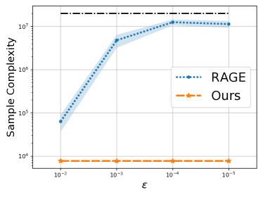
Figure 1: Comparison of Sample Complexity

The success rates of RAGE and our algorithm are shown in Table 1. The success rate of RAGE drops dramatically as $\varepsilon$ (the smallest sub-optimality gap) gets smaller. On the other hand, however, our algorithm is not affected by the change of $\varepsilon$ since it automatically adapts to the intrinsic dimension $d_{\star}$: One can immediately see that $h(x_{d_{\star}})\geq h(x_{d_{\star}+1})$ when working in ${\mathbb{R}}^{d_{\star}}$. Due to the same reason, our algorithm significantly outperforms RAGE in sample complexity as well (see Fig. 1): Our algorithm adapts to the true sample complexity $\rho^{\star}_{d_{\star}}$ yet RAGE suffers from complexity $\rho^{\star}_{D}\gg\rho^{\star}_{d_{\star}}$, especially when $\varepsilon$ is small.

The runtime of both algorithms are shown in Table 2. Our algorithm is affected by the computational overhead of conducting model selection (e.g., the two dimensional doubling trick). Thus, RAGE shows advantages in runtime when $\varepsilon$ is relatively large. However, our algorithm runs faster than RAGE when $\varepsilon$ gets smaller. This observation further shows that the implementation overhead can be small in comparison with the sample complexity gains achieved from model selection.

Table 2: Comparison of Runtime

$\varepsilon$	$10^{-2}$	$10^{-3}$	$10^{-4}$	$10^{-5}$
RAGE	$3.46\,$s	$7.87\,$s	$17.33\,$s	$16.81\,$s
Ours	$12.12\,$s	$11.17\,$s	$12.44\,$s	$12.41\,$s

It is worth mentioning that simple variations of the problem instance studied in this section have long been considered as hard instances to examine linear bandit pure exploration algorithms (Soare et al., 2014; Xu et al., 2018; Tao et al., 2018; Fiez et al., 2019; Degenne et al., 2020). Our results show that, both theoretically and empirically, the problem instance becomes quite easy when viewed from the model selection perspective.

8 DISCUSSION

We initiate the study of model selection in pure exploration linear bandits, in both fixed confidence and fixed budget settings, and design algorithms with near instance optimal guarantees. Along the way, we develop a novel selection-validation procedure to deal with the understudied fixed budget setting in linear bandits (even without the added challenge of model selection). We also adapt our algorithms to problems with model misspecification.

We conclude the paper with some directions for future work. An immediate next step is to conduct large-scale evaluations for model selection in pure exploration linear bandits. One may need to develop practical version of our algorithms to bypass the computational overheads of conducting model selection. Another interesting direction is provide guarantees to general transductive linear bandits, i.e., not restricted to cases $\mathcal{Z}\subseteq\mathcal{X}$, in fixed budget setting/misspecified regime. We believe one can use a selection-validation procedure similar to the one developed in Algorithm 3, but with the current validation step replaced by another linear bandit pure exploration algorithm. Note that the number of arms to be validated is of logarithmic order.

Acknowledgements

We thank anonymous reviewers for helpful comments. This work is partially supported by NSF grant 1934612 and ARMY MURI grant W911NF-15-1-0479.

 

Supplementary Material:
Near Instance Optimal Model Selection for Pure Exploration Linear Bandits

 

Appendix A SUPPORTING MATERIALS

A.1 Matrix Inversion and Rounding in Optimal Design

Our treatments are similar to the ones discussed in Zhu et al. (2021). We provide the details here for completeness.

Matrix Inversion. The notation $\left\lVert y\right\rVert^{2}_{A_{d}(\lambda)^{-1}}$ is clear when $A_{d}(\lambda)$ is invertible. For possibly singular $A_{d}(\lambda)$, pseudo-inverse is used if $y$ belongs to the range of $A_{d(\lambda)}$; otherwise, we set $\left\lVert y\right\rVert_{A_{d}(\lambda)^{-1}}^{2}=\infty$. With this (slightly abused) definition of matrix inversion, we discuss how to do rounding next.

Rounding in Optimal Design. For any ${\mathcal{S}}\subseteq\mathcal{Z}$, the following optimal design

$$\inf_{\lambda\in\mathbf{\Lambda}_{\mathcal{X}}}\sup_{y\in\mathcal{Y}(\psi_{d}({\mathcal{S}}))}\left\lVert y\right\rVert^{2}_{A_{d}(\lambda)^{-1}}$$

will select a design $\lambda^{\star}\in\mathbf{\Lambda}_{\mathcal{X}}$ such that every $y\in\mathcal{Y}(\psi_{d}({\mathcal{S}}))$ lies in the range of $A_{d}(\lambda^{\star})$. If $\operatorname{span}(\mathcal{Y}(\psi_{d}({\mathcal{S}})))={\mathbb{R}}^{d}$, then $A_{{}_{d}}(\lambda^{\star})$ is positive definite (recall that $A_{d}(\lambda^{\star})=\sum_{x\in\mathcal{X}}\lambda_{x}\psi_{d}(x)\psi_{d}(x)^{\top}$ and $\operatorname{span}(\psi_{d}(\mathcal{X}))={\mathbb{R}}^{d}$ comes from the assumption that $\operatorname{span}(\psi(\mathcal{X}))={\mathbb{R}}^{D}$). Thus the rounding guarantees in Allen-Zhu et al. (2020) goes through (Theorem 2.1 therein, which requires a positive definite design; with additional simple modifications dealt as in Appendix B of Fiez et al. (2019)).

We now consider the case when $A_{d}(\lambda^{\star})$ is singular. Since $\operatorname{span}(\psi_{d}(\mathcal{X}))={\mathbb{R}}^{d}$, we can always find another $\lambda^{\prime}$ such that $A_{d}(\lambda^{\prime})$ is invertible. For any $\zeta_{1}>0$, let $\widetilde{\lambda}^{\star}=(1-\zeta_{1})\lambda^{\star}+\zeta_{1}\lambda^{\prime}$. We know that $\widetilde{\lambda}^{\star}$ leads to a positive definite design. With respect to $\zeta_{1}$, we can find another $\zeta_{2}>0$ small enough (e.g., smaller than the smallest eigenvalue of $\zeta_{1}A_{d}(\lambda^{\prime})$) such that $A_{d}(\widetilde{\lambda}^{\star})\succeq A_{d}((1-\zeta_{1})\lambda^{\star})+\zeta_{2}I$. Since $A_{d}((1-\zeta_{1})\lambda^{\star})+\zeta_{2}I$ is positive definite, for any $y\in\mathcal{Y}(\psi_{d}({\mathcal{S}}))$, we have

$$\left\lVert y\right\rVert^{2}_{A_{d}(\widetilde{\lambda}^{\star})^{-1}}\leq\left\lVert y\right\rVert^{2}_{(A_{d}((1-\zeta_{1})\lambda^{\star})+\zeta_{2}I)^{-1}}.$$

Fix any $y\in\mathcal{Y}(\psi_{d}({\mathcal{S}}))$. Since $y$ lies in the range of $A_{d}(\lambda^{\star})$ (by definition of the objective and matrix inversion), we clearly have

$$\left\lVert y\right\rVert^{2}_{(A_{d}((1-\zeta_{1})\lambda^{\star})+\zeta_{2}I)^{-1}}\leq\left\lVert y\right\rVert^{2}_{(A_{d}((1-\zeta_{1})\lambda^{\star}))^{-1}}\leq\frac{1}{1-\zeta_{1}}\left\lVert y\right\rVert^{2}_{A_{d}(\lambda^{\star})^{-1}}.$$

To summarize, we have

$$\left\lVert y\right\rVert^{2}_{A_{d}(\widetilde{\lambda}^{\star})^{-1}}\leq\frac{1}{1-\zeta_{1}}\left\lVert y\right\rVert^{2}_{A_{d}(\lambda^{\star})^{-1}},$$

where $\zeta_{1}$ can be chosen arbitrarily small. We can thus send the positive definite design $\widetilde{\lambda}^{\star}$ to the rounding procedure in Allen-Zhu et al. (2020). We can incorporate the additional $1/(1-\zeta_{1})$ overhead, for $\zeta_{1}>0$ chosen sufficiently small, into the sample complexity requirement $r_{d}(\zeta)$ of the rounding procedure.

A.2 Supporting Theorems and Lemmas

Lemma 3 ((Kaufmann et al., 2016)).

Fixed any pure exploration algorithm $\pi$. Let $\nu$ and $\nu^{\prime}$ be two bandit instances with $K$ arms such that the distribution $\nu_{i}$ and $\nu_{i}^{\prime}$ are mutually absolutely continuous for all $i\in[K]$. For any almost-surely finite stopping time $\tau$ with respect to the filtration $\left\{\mathcal{F}_{t}\right\}_{t\geq 0}$, let $N_{i}(\tau)$ be the number of pulls on arm $i$ at time $\tau$. We then have

$$\sum_{i=1}^{K}{\mathbb{E}}_{\nu}[N_{i}(\tau)]\operatorname{KL}\left(\nu_{i},\nu_{i}^{\prime}\right)\geq\sup_{\mathcal{E}\in\mathcal{F}_{\tau}}d\left({\mathbb{P}}_{\nu}(\mathcal{E}),{\mathbb{P}}_{\nu^{\prime}}(\mathcal{E})\right),$$

where $d(x,y)=x\log(x/y)+(1-x)\log((1-x)/(1-y))$ for $x,y\in[0,1]$ and with the convention that $d(0,0)=d(1,1)=0$.

The following two lemmas largely follow the analysis in Fiez et al. (2019).

Lemma 4.

Let ${\mathcal{S}}_{k}=\{z\in\mathcal{Z}:\Delta_{z}<4\cdot 2^{-k}\}$. We then have

$$\sup_{k\in[\left\lfloor\log_{2}\left(4/\varepsilon\right)\right\rfloor]}\{2^{2k}\iota\left(\mathcal{Y}(\psi_{d}({\mathcal{S}}_{k}))\right)\}\leq 64\rho_{d}^{\star}(\varepsilon),$$ (6)

and

$$\sup_{k\in[\left\lfloor\log_{2}\left(4/\varepsilon\right)\right\rfloor]}\{\max\{2^{2k}\iota\left(\mathcal{Y}(\psi_{d}({\mathcal{S}}_{k}))\right),r_{d}(\zeta)\}\}\leq\max\left\{64\rho_{d}^{\star}(\varepsilon),r_{d}(\zeta)\right\},$$ (7)

where $\zeta$ is the rounding parameter.

Proof.

For $y=\psi_{d}(z_{\star})-\psi_{d}(z)$, we define $\Delta_{y}=\Delta_{z}=h(z_{\star})-h(z)$. We have that

$$\rho_{d}^{\star}(\varepsilon) =\inf_{\lambda\in\mathbf{\Lambda}_{\mathcal{X}}}\sup_{y\in\mathcal{Y}^{\star}(\psi_{d}(\mathcal{Z}))}\frac{\left\lVert y\right\rVert^{2}_{A_{d}(\lambda)^{-1}}}{\max\{\Delta_{y},\varepsilon\}^{2}}$$

$$=\inf_{\lambda\in\mathbf{\Lambda}_{\mathcal{X}}}\sup_{k\in[\left\lfloor\log_{2}\left(4/\varepsilon\right)\right\rfloor]}\sup_{y\in\mathcal{Y}^{\star}(\psi_{d}({\mathcal{S}}_{k}))}\frac{\left\lVert y\right\rVert^{2}_{A_{d}(\lambda)^{-1}}}{\max\{\Delta_{y},\varepsilon\}^{2}}$$

$$\geq\sup_{k\in[\left\lfloor\log_{2}\left(4/\varepsilon\right)\right\rfloor]}\inf_{\lambda\in\mathbf{\Lambda}_{\mathcal{X}}}\sup_{y\in\mathcal{Y}^{\star}(\psi_{d}({\mathcal{S}}_{k}))}\frac{\left\lVert y\right\rVert^{2}_{A_{d}(\lambda)^{-1}}}{\max\{\Delta_{y},\varepsilon\}^{2}}$$

$$>\sup_{k\in[\left\lfloor\log_{2}\left(4/\varepsilon\right)\right\rfloor]}\inf_{\lambda\in\mathbf{\Lambda}_{\mathcal{X}}}\sup_{y\in\mathcal{Y}^{\star}(\psi_{d}({\mathcal{S}}_{k}))}\frac{\left\lVert y\right\rVert^{2}_{A_{d}(\lambda)^{-1}}}{\left(4\cdot 2^{-k}\right)^{2}}$$ (8)

$$\geq\sup_{k\in[\left\lfloor\log_{2}\left(4/\varepsilon\right)\right\rfloor]}\inf_{\lambda\in\mathbf{\Lambda}_{\mathcal{X}}}\sup_{y\in\mathcal{Y}(\psi_{d}({\mathcal{S}}_{k}))}\frac{\left\lVert y\right\rVert^{2}_{A_{d}(\lambda)^{-1}}/4}{\left(4\cdot 2^{-k}\right)^{2}}$$ (9)

$$\geq\sup_{k\in[\left\lfloor\log_{2}\left(4/\varepsilon\right)\right\rfloor]}2^{2k}\iota(\mathcal{Y}(\psi_{d}({\mathcal{S}}_{k})))/64,$$

where Eq. 8 comes from the fact that $4\cdot 2^{-k}\geq\varepsilon$ when $k\leq\lfloor\log_{2}(4/\varepsilon)\rfloor$; Eq. 9 comes from the fact that $\psi_{d}(z)-\psi_{d}(z^{\prime})=(\psi_{d}(z)-\psi_{d}(z_{\star}))+(\psi_{d}(z_{\star})-\psi_{d}(z^{\prime}))$. This implies that, for any $k\in[\left\lfloor\log_{2}\left(4/\varepsilon\right)\right\rfloor]$,

$$\max\left\{2^{2k}\rho(\mathcal{Y}(\psi_{d}({\mathcal{S}}_{k}))),r_{d}(\zeta)\right\}\leq\max\left\{64\rho_{d}^{\star}(\varepsilon),r_{d}(\zeta)\right\}.$$

And the desired Eq. 7 immediately follows. ∎

Lemma 5.

Let ${\mathcal{S}}_{k}=\{z\in\mathcal{Z}:\Delta_{z}<4\cdot 2^{-k}\}$. We then have

$$\sup_{k\in[\left\lceil\log_{2}\left(4/\Delta_{\min}\right)\right\rceil]}\{2^{2k}\iota\left(\mathcal{Y}(\psi_{d}({\mathcal{S}}_{k}))\right)\}\leq 64\rho_{d}^{\star},$$ (10)

and

$$\sup_{k\in[\left\lceil\log_{2}\left(4/\Delta_{\min}\right)\right\rceil]}\{\max\{2^{2k}\iota\left(\mathcal{Y}(\psi_{d}({\mathcal{S}}_{k}))\right),r_{d}(\zeta)\}\}\leq\max\left\{64\rho_{d}^{\star},r_{d}(\zeta)\right\},$$ (11)

where $\zeta$ is the rounding parameter.

Proof.

Take $\varepsilon=\Delta_{\min}$ in Lemma 4. ∎

The following lemma largely follows the analysis in Soare et al. (2014), with generalization to the transductive setting and more careful analysis in terms of matrix inversion.

Lemma 6.

Fix $\mathcal{Z}\subseteq\mathcal{X}\subseteq{\mathbb{R}}^{D}$. Suppose $\max_{x\in\mathcal{X}}\left\lVert x\right\rVert^{2}\leq c_{1}$ and $\min_{z\in\mathcal{Z}\setminus\{z_{\star}\}}\left\lVert z_{\star}-z\right\rVert^{2}\geq c_{2}$ with some absolute constant $c_{1}$ and $c_{2}$. We have

$$\frac{c_{2}}{c_{1}\Delta_{\min}^{2}}\leq\rho^{\star}\vcentcolon=\inf_{\lambda\in\mathbf{\Lambda}_{\mathcal{X}}}\sup_{z\in\mathcal{Z}\setminus\{z_{\star}\}}\frac{\lVert z_{\star}-z\rVert^{2}_{A(\lambda)^{-1}}}{\Delta_{z}^{2}},$$

where $\Delta_{\min}=\min_{z\in\mathcal{Z}\setminus\left\{z_{\star}\right\}}\left\{\Delta_{z}\right\}$.

Proof.

Let $\lambda^{\star}$ be the optimal design that attains $\rho^{\star}$; and let $z^{\prime}\in\mathcal{Z}$ be any arm with the smallest sub-optimality gap $\Delta_{\min}$. We then have

$$\rho^{\star} =\max_{z\in\mathcal{Z}\setminus\{z_{\star}\}}\frac{\lVert z_{\star}-z\rVert^{2}_{A(\lambda^{\star})^{-1}}}{\Delta_{z}^{2}}$$

$$\geq\frac{\lVert z_{\star}-z^{\prime}\rVert^{2}_{A(\lambda^{\star})^{-1}}}{\Delta_{z^{\prime}}^{2}}$$

$$=\frac{\lVert z_{\star}-z^{\prime}\rVert^{2}_{A(\lambda^{\star})^{-1}}}{\Delta_{\min}^{2}},$$ (12)

where $z_{\star}-z^{\prime}$ necessarily lie in the range of $A(\lambda^{\star})$ according to the definition of matrix inversion in Section A.1.

We now lower bound $\lVert z_{\star}-z^{\prime}\rVert^{2}_{A(\lambda^{\star})^{-1}}$. Note that $A(\lambda^{\star})$ is positive semi-definite. We write $A(\lambda^{\star})=Q\Sigma Q^{\top}$ where $Q$ is an orthogonal matrix and $\Sigma$ is a diagonal matrix storing eigenvalues. We assume that the last $k$ eigenvalues of $\Sigma$ are zero. Let $\gamma_{\max}=\left\lVert A(\lambda^{\star})\right\rVert_{2}=\left\lVert\Sigma\right\rVert_{2}$ be the largest eigenvalue, we have $\gamma_{\max}\leq\max_{x\in\mathcal{X}}\left\lVert x\right\rVert^{2}\leq c_{1}$ since $A(\lambda^{\star})=\sum_{x\in\mathcal{X}}\lambda^{\star}(x)xx^{\top}$ and $\sum_{x\in\mathcal{X}}\lambda^{\star}(x)=1$. Let $w=Q^{\top}(z_{\star}-z^{\prime})$. Since $z_{\star}-z^{\prime}$ is in the range of $A(\lambda^{\star})$, we know that the last $k$ entries of $w$ must be zero. We then have

$$\lVert z_{\star}-z^{\prime}\rVert^{2}_{A(\lambda^{\star})^{-1}} =(z_{\star}-z)^{\top}A(\lambda^{\star})^{-1}(z_{\star}-z)$$

$$=w^{\top}\Sigma^{-1}w$$

$$\geq{\left\lVert w\right\rVert^{2}}/{c_{1}}$$

$$\geq c_{2}/c_{1},$$ (13)

where Eq. 13 comes from fact that $\left\lVert w\right\rVert^{2}=\left\lVert z_{\star}-z^{\prime}\right\rVert^{2}$ and the assumption $\left\lVert z_{\star}-z\right\rVert^{2}\geq c_{2}$ for all $z\in\mathcal{Z}$. ∎

Lemma 7.

The following statements hold.

1. $T\geq 4a\log 2a\implies T\geq a\log_{2}T$ for $T,a>0$.

2. $T\geq 16a\,(\log 16a)^{2}\implies T\geq a\,(\log_{2}T)^{2}$ for $T,a>1$.

Proof.

We first recall that $T\geq 2a\log a\implies T\geq a\log T$ for $T,a>0$ (Shalev-Shwartz and Ben-David, 2014). Since $\log_{2}T=\log T/\log 2<2\log T$, the first statement immediately follows.

To prove the second statement, we only need to find conditions on $T$ such that $T\geq 4a\,(\log T)^{2}$. Note that we have $\sqrt{T}\geq 8\sqrt{a}\log 4\sqrt{a}=4\sqrt{a}\log 16a\implies\sqrt{T}\geq 4\sqrt{a}\log\sqrt{T}=2\sqrt{a}\log T$. For $T,a>1$, this is equivalent to $T\geq 16a\,(\log 16a)^{2}\implies T\geq 4a\,(\log T)^{2}\geq a\,(\log_{2}T)^{2}$, and thus the second statement follows. ∎

A.3 Supporting Algorithms

Algorithm 5 OPT

0:  Selection budget $B$, dimension upper bound $D$ and selection function $g(\cdot)$ (which is a function of the dimension $d\in[D]$).

1:  Get $d_{k}$ such that

$$d_{k}= \max d$$

$$\text{ s.t. }g(d)\leq B,\text{ and }d\in[D].$$

1:  The selected dimension $d_{k}$.

Appendix B OMITTED PROOFS FOR SECTION 3

B.1 Proof of Theorem 1

See 1

Proof.

The proof of the theorem mostly follows the proof of lower bound in Fiez et al. (2019). We additionally consider the model selection problem $(\mathcal{X},\mathcal{Z}$, $\theta_{\star}\in\Theta_{d_{\star}})$ and carefully deal with the matrix inversion.

Consider the instance $(\mathcal{X},\mathcal{Z}$, $\theta_{\star}\in\Theta_{d_{\star}})$, where $\mathcal{X}=\{x_{1},\ldots,x_{n}\}$ and $\operatorname{span}(\mathcal{X})={\mathbb{R}}^{D}$, $\mathcal{Z}=\{z_{1},\ldots,z_{m}\}$. Suppose that $z_{1}=\operatorname*{arg\,max}_{z\in\mathcal{Z}}\langle\theta_{\star},z\rangle$. We consider the alternative set $\mathcal{C}_{d_{\star}}\vcentcolon=\{\theta\in\Theta_{d_{\star}}:\exists i\in[m]\text{ s.t. }\langle\theta,z_{1}-z_{i}\rangle<0\}$, where $z_{1}$ is not the best arm for any $\theta\in\mathcal{C}_{d_{\star}}$. Following the “change of measure” argument in Lemma 3, we know that ${\mathbb{E}}_{\theta_{\star}}[\tau]\geq\tau^{\star}$, where $\tau^{\star}$ is the solution of the following constrained optimization

$$\tau^{\star} \vcentcolon=\min_{t_{1},\dots,t_{n}\in{\mathbb{R}}_{+}}\sum_{i=1}^{n}t_{i}$$ (14)

$$\qquad\text{ s.t. }\inf_{\theta\in\mathcal{C}_{d_{\star}}}\sum_{i=1}^{n}t_{i}\operatorname{KL}(\nu_{\theta_{\star},i},\nu_{\theta,i})\geq\log(1/2.4\delta),$$

where we use the notation $\nu_{\theta,i}=\mathcal{N}(\langle\theta,x_{i}\rangle,1)=\mathcal{N}(\langle\psi_{d_{\star}}(\theta),\psi_{d_{\star}}(x_{i})\rangle,1)$ (due to the fact that $\theta\in\mathcal{C}_{d_{\star}}$). We also have $\operatorname{KL}(\nu_{\theta_{\star},i},\nu_{\theta,i})=\frac{1}{2}\langle\psi_{d_{\star}}(\theta_{\star})-\psi_{d_{\star}}(\theta),\psi_{d_{\star}}(x_{i})\rangle^{2}$.

We next show that for any $t=(t_{1},\dots,t_{n})^{\top}\in{\mathbb{R}}_{+}^{n}$ satisfies the constraint of Eq. 14, we must have $\psi_{d_{\star}}(z_{1})-\psi_{d_{\star}}(z_{i})\in\operatorname{span}(\{\psi_{d_{\star}}(x_{i}):t_{i}>0\}),\forall\,2\leq i\leq m$. Suppose not, there must exists a $\psi_{d_{\star}}(u)\in{\mathbb{R}}^{d_{\star}}$ such that (1) $\langle\psi_{d_{\star}}(u),\psi_{d_{\star}}(x_{i})\rangle=0$ for all $i\in[n]$ such that $t_{i}>0$; and (2) there exists a $2\leq j\leq m$ such that $\langle\psi_{d_{\star}}(z_{1})-\psi_{d_{\star}}(z_{j}),\psi_{d_{\star}}(u)\rangle\neq 0$. Suppose $\langle\psi_{d_{\star}}(z_{1})-\psi_{d_{\star}}(z_{j}),\psi_{d_{\star}}(u)\rangle>0$ (the other direction is similar), we can choose a $\theta^{\prime}\in\Theta_{d_{\star}}$ such that the first $d_{\star}$ coordinates of $\theta^{\prime}$ equals to $\psi_{d_{\star}}(\theta_{\star})-\alpha\,\psi_{d_{\star}}(u)$ for a $\alpha>0$ large enough (so that $\theta^{\prime}\in\mathcal{C}_{d_{\star}}$). With such $\theta^{\prime}$, however, we have

$$\sum_{i=1}^{n}t_{i}\operatorname{KL}(\nu_{\theta_{\star},i},\nu_{\theta^{\prime},i})=\sum_{i=1}^{n}t_{i}\frac{1}{2}\langle\alpha\,\psi_{d_{\star}}(u),\psi_{d_{\star}}(x_{i})\rangle^{2}=0<\log(1/2.4\delta),$$

which leads to a contradiction. As a result, we can safely calculate $\left\lVert\psi_{d_{\star}}(z_{1})-\psi_{d_{\star}}(z_{i})\right\rVert^{2}_{A_{d_{\star}}(t)^{-1}}$ or $A_{d_{\star}}(t)^{-1}(\psi_{d_{\star}}(z_{1})-\psi_{d_{\star}}(z_{i}))$ where $A_{d_{\star}}(t)\vcentcolon=\sum_{i=1}^{n}t_{i}\psi_{d_{\star}}(x_{i})\psi_{d_{\star}}(x_{i})^{\top}/\bar{t}$ and $\bar{t}\vcentcolon=\sum_{i=1}^{n}t_{i}$. The rest of the proof follows from the proof of theorem 1 in Fiez et al. (2019). ∎

B.2 Proof of Theorem 2

See 2

Proof.

The proof largely follows from the proof of Theorem 3 in Katz-Samuels et al. (2020) (but ignore the $\gamma^{\star}$ term therein. We are effectively using a weaker lower bound, yet it suffices for our purpose. ). The non-interactive MLE uses at least $\frac{1}{2}\rho^{\star}_{d}\log(1/\delta)$ with respect to any feature mapping $\psi_{d}(\cdot)$ for $d_{\star}\leq d\leq D$. The statement then follows from the monotonicity of $\{\rho^{\star}_{d}\}_{d=d_{\star}}^{D}$ as shown in Proposition 1. ∎

B.3 Proof of Proposition 1

See 1

Proof.

We first prove equivalence results in the general setting in Step 1, 2 and 3; and then apply the results to the model selection problem in Step 4 to prove monotonicity over $\{\rho_{d}^{\star}\}_{d=d_{\star}}^{D}$.

We consider instance $(\mathcal{X},\mathcal{Z}$, $\theta_{\star})$ in the general setting, where $\mathcal{X}=\{x_{1},\ldots,x_{n}\}\subseteq{\mathbb{R}}^{d}$, $\operatorname{span}(\mathcal{X})={\mathbb{R}}^{d}$, $\mathcal{Z}=\{z_{1},\ldots,z_{m}\}$ and $\theta_{\star}\in{\mathbb{R}}^{d}$. We suppose that $z_{1}=\operatorname*{arg\,max}_{z\in\mathcal{Z}}\langle\theta_{\star},z\rangle$ is the unique optimal arm and $\operatorname{span}(\{z_{1}-z\}_{z\in\mathcal{Z}\setminus\{z_{1}\}})={\mathbb{R}}^{d}$. We use the notations $y_{j}\vcentcolon=z_{1}-z_{j}$ for $j=2,\ldots,m$, and $\nu_{\theta,i}\vcentcolon=\mathcal{N}(x_{i}^{\top}\theta,1)$. For any $t=(t_{1},\ldots,t_{n})^{\top}\in{\mathbb{R}}^{n}_{+}$, we also use the notation $A(t)=\sum_{i=1}^{n}t_{i}x_{i}x_{i}^{\top}\in{\mathbb{R}}^{d\times d}$ to denote a design matrix with respect to $t$ ($t$ doesn’t need to be inside the simplex $\mathbf{\Lambda}_{\mathcal{X}}$). We consider any fixed $\delta\in(0,0.15]$.

Step 1: Closure of constraints. Let $\mathcal{C}$ denote the set of parameters where $z_{1}$ is no longer the best arm anymore, i.e.,

$$\mathcal{C} \vcentcolon=\{\theta\in{\mathbb{R}}^{d}:\exists i\in[m]\text{ s.t. }\theta^{\top}(z_{1}-z_{i})<0\}.$$

Using the “change of measure” argument from Kaufmann et al. (2016), the lower bound is given by the following optimization problem (Audibert et al., 2010; Fiez et al., 2019)

$$\tau^{\star} :=\min_{t_{1},\ldots,t_{n}\in{\mathbb{R}}_{+}}\sum_{i=1}^{n}t_{i}$$

$$\qquad\text{ s.t. }\inf_{\theta\in\mathcal{C}}\sum_{i=1}^{n}t_{i}\operatorname{KL}(\nu_{\theta_{\star},i},\nu_{\theta,i})\geq\log(1/2.4\delta).$$

First, we show that the value $\tau^{\star}$ equals to the value of another optimization problem, i.e.,

$$\tau^{\star} =\min_{t_{1},\ldots,t_{n}\in{\mathbb{R}}_{+}}\sum_{i=1}^{n}t_{i}$$

$$\qquad\text{ s.t. }\min_{\theta\in\bar{\mathcal{C}}}\sum_{i=1}^{n}t_{i}\operatorname{KL}(\nu_{\theta_{\star},i},\nu_{\theta,i})\geq\log(1/2.4\delta),$$

where $\bar{\mathcal{C}}=\{\theta\in{\mathbb{R}}^{d}:\exists i\in[m]\text{ s.t. }\theta^{\top}(z_{1}-z_{i})\leq 0\}$. Note that that we must show that the minimum in the constraint is attained, i.e., the $\min_{\theta\in\bar{\mathcal{C}}}$ part. We first show the equivalence between the original problem and the problem with respect to $\inf_{\theta\in\bar{\mathcal{C}}}$; and then show the equivalence between problems with respect to $\inf_{\theta\in\bar{\mathcal{C}}}$ and $\min_{\theta\in\bar{\mathcal{C}}}$. We fix any $t=(t_{1},\ldots,t_{n})^{\top}\in{\mathbb{R}}^{n}_{+}$.

Step 1.1: We claim that $\inf_{\theta\in\mathcal{C}}\sum_{i=1}^{n}t_{i}\operatorname{KL}(\nu_{\theta_{\star},i},\nu_{\theta,i})\geq\log(1/2.4\delta)$ if and only if $\inf_{\theta\in\bar{\mathcal{C}}}\sum_{i=1}^{n}t_{i}\operatorname{KL}(\nu_{\theta_{\star},i},\nu_{\theta,i})\geq\log(1/2.4\delta)$.

Since $\bar{\mathcal{C}}\supset\mathcal{C}$, the $\Longleftarrow$ direction is obvious.

Now, suppose $\inf_{\theta\in\bar{\mathcal{C}}}\sum_{i=1}^{n}t_{i}\operatorname{KL}(\nu_{\theta_{\star},i},\nu_{\theta,i})<\log(1/2.4\delta)$. By definition of $\inf$, there exists $\theta_{0}\in\bar{\mathcal{C}}$ such that

$$\sum_{i=1}^{n}t_{i}\operatorname{KL}(\nu_{\theta_{\star},i},\nu_{\theta_{0},i})<\log(1/2.4\delta).$$

Since $\bar{\mathcal{C}}$ is the closure of an open set $\mathcal{C}$, there exists a sequence $\{\theta_{j}\}$ in $\mathcal{C}$ approaching $\theta_{0}$. Note that

$$\sum_{i=1}^{n}t_{i}\operatorname{KL}(\nu_{\theta_{\star},i},\nu_{\theta,i})=\sum_{i=1}^{n}t_{i}\frac{1}{2}(x_{i}^{\top}(\theta_{\star}-\theta))^{2}=\frac{1}{2}\left\lVert\theta_{\star}-\theta\right\rVert_{A(t)}^{2}.$$

Then, by the continuity of $\frac{1}{2}\left\lVert\theta_{\star}-\theta\right\rVert_{A(t)}^{2}$ in $\theta$, there exists a $\theta\in\mathcal{C}$ such that $\sum_{i=1}^{n}t_{i}\operatorname{KL}(\nu_{\theta_{\star},i},\nu_{\theta,i})<\log(1/2.4\delta)$. This gives a contradiction and thus proves the $\Longrightarrow$ direction.

Step 1.2: Now, we must show that the infimum is attained whenever $\inf_{\theta\in\bar{\mathcal{C}}}\sum_{i=1}^{n}t_{i}\operatorname{KL}(\nu_{\theta_{\star},i}||\nu_{\theta,i})\geq\log(1/2.4\delta)$, that is, there exists $\theta_{0}\in\bar{\mathcal{C}}$ such that

$$\sum_{i=1}^{n}t_{i}\operatorname{KL}(\nu_{\theta_{\star},i},\nu_{\theta_{0},i}) =\inf_{\theta\in\bar{\mathcal{C}}}\sum_{i=1}^{n}t_{i}\operatorname{KL}(\nu_{\theta_{\star},i},\nu_{\theta,i}).$$

Claim: Fix $t=(t_{1},\ldots,t_{n})^{\top}\in{\mathbb{R}}_{+}^{n}$. If $\operatorname{span}(\{x_{i}:t_{i}>0\})\neq{\mathbb{R}}^{d}$, then $\inf_{\theta\in\bar{\mathcal{C}}}\sum_{i=1}^{n}t_{i}\operatorname{KL}(\nu_{\theta_{\star},i},\nu_{\theta,i})<\log(1/2.4\delta)$.

First, we show the claim. Fix $t=(t_{1},\ldots,t_{n})^{\top}\in{\mathbb{R}}_{+}^{n}$ and suppose $\operatorname{span}(\{x_{i}:t_{i}>0\})\neq{\mathbb{R}}^{d}$. Since $\operatorname{span}(\{x_{i}:t_{i}>0\})\neq{\mathbb{R}}^{d}$, there exists $u\in{\mathbb{R}}^{d}$ such that $u^{\top}x_{i}=0$ for all $i$ such that $t_{i}>0$. Since $\{z_{1}-z_{i}:i\in[m]\}$ spans ${\mathbb{R}}^{d}$ by assumption, there exists $i\in[m]$ such that $u^{\top}(z_{1}-z_{i})\neq 0$. Suppose that $u^{\top}(z_{1}-z_{i})<0$ (the other case is similar). Then, there exists a sufficiently large $\alpha>0$ such that $(\theta_{\star}+\alpha u)^{\top}(z_{1}-z_{i})<0$, implying that $\theta_{\star}+\alpha u\in\mathcal{C}$. Moreover, by construction of $u$, we have

$$\sum_{i=1}^{n}t_{i}\operatorname{KL}(\nu_{\theta_{\star},i},\nu_{\theta_{\star}+\alpha u,i}) =\sum_{i=1}^{n}t_{i}\frac{1}{2}(x_{i}^{\top}(\alpha u))^{2}=\sum_{i:t_{i}>0}t_{i}\frac{1}{2}(x_{i}^{\top}(\alpha u))^{2}=0<\log(1/2.4\delta),$$

and thus leads to the claim.

Now, suppose $\inf_{\theta\in\bar{\mathcal{C}}}\sum_{i=1}^{n}t_{i}\operatorname{KL}(\nu_{\theta_{\star},i},\nu_{\theta,i})\geq\log(1/2.4\delta)$. Then, $\operatorname{span}(\{x_{i}:t_{i}>0\})={\mathbb{R}}^{d}$. Then, $\left\lVert\cdot\right\rVert_{A(t)}^{2}$ is a norm, and the set

$$\left\{\theta\in{\mathbb{R}}^{d}:\frac{1}{2}\left\lVert\theta-\theta_{\star}\right\rVert_{A(t)}^{2}\leq\varepsilon\right\}$$

is compact for every $\varepsilon$. Then, since $\bar{\mathcal{C}}$ is closed and $\frac{1}{2}\left\lVert\theta-\theta_{\star}\right\rVert_{A(t)}^{2}$ has compact sublevel sets, there exists a $\theta_{0}\in\bar{\mathcal{C}}$ such that

$$\sum_{i=1}^{n}t_{i}\operatorname{KL}(\nu_{\theta_{\star},i},\nu_{\theta_{0},i})=\inf_{\theta\in\bar{\mathcal{C}}}\sum_{i=1}^{n}t_{i}\operatorname{KL}(\nu_{\theta_{\star},i},\nu_{\theta,i}).$$

This shows the equivalence between problems with respect to $\inf_{\theta\in\bar{\mathcal{C}}}$ and $\min_{\theta\in\bar{\mathcal{C}}}$.

Step 2: Rewrite the optimization problem. Define

$$\bar{\mathcal{C}}_{i} =\{\theta\in{\mathbb{R}}^{d}:\theta^{\top}(z_{1}-z_{i})\leq 0\},$$

and note that $\bar{\mathcal{C}}=\cup_{i=1}^{m}\bar{\mathcal{C}}_{i}$. Observe that

$$\tau^{\star} :=\min_{t_{1},\ldots,t_{n}\in{\mathbb{R}}_{+}}\sum_{i=1}^{n}t_{i}$$

$$\qquad\text{ s.t. }\min_{\theta\in\bar{\mathcal{C}}}\sum_{i=1}^{n}t_{i}\operatorname{KL}(\nu_{\theta_{\star},i},\nu_{\theta,i})\geq\log(1/2.4\delta)$$

$$=\min_{t_{1},\ldots,t_{n}\in{\mathbb{R}}_{+}}\sum_{i=1}^{n}t_{i}$$

$$\qquad\text{ s.t. }\min_{i\in[m]}\min_{\theta\in\bar{\mathcal{C}}_{i}}\sum_{i=1}^{n}t_{i}\operatorname{KL}(\nu_{\theta_{\star},i},\nu_{\theta,i})\geq\log(1/2.4\delta).$$

Consider the optimization problem:

$$\min_{\theta\in\bar{\mathcal{C}}_{i}} \frac{1}{2}\sum_{i=1}^{n}t_{i}(x_{i}^{\top}(\theta_{\star}-\theta))^{2}=\min_{\theta\in\bar{\mathcal{C}}_{i}}\frac{1}{2}\left\lVert\theta_{\star}-\theta\right\rVert_{A(t)}^{2}$$

Note that since the objective is convex and there exists $\theta\in{\mathbb{R}}^{d}$ such that $\theta^{\top}(z_{1}-z_{i})<0$, Slater’s condition holds and, therefore, strong duality holds. We form the Lagrangian with lagrange multiplier $\gamma\in{\mathbb{R}}_{+}$ to obtain

$$\L(\theta,\gamma) =\frac{1}{2}\left\lVert\theta_{\star}-\theta\right\rVert_{A(t)}^{2}+\gamma\cdot y_{i}^{\top}\theta$$

Differentiating with respect to $\theta$ and $\gamma$, we have that (note that $A(t)$ is invertible from the claim in Step 1)

$$\begin{cases}\theta&=\theta_{\star}-\gamma A(t)^{-1}y_{i},\\ y_{i}^{\top}\theta&=0.\end{cases}$$

These imply that $\theta_{0}\vcentcolon=\theta_{\star}-\frac{y_{i}^{\top}\theta_{\star}A(t)^{-1}y_{i}}{y_{i}^{\top}A(t)^{-1}y_{i}}$ and $\gamma_{0}\vcentcolon=\frac{y_{i}\top\theta_{\star}}{y_{i}^{\top}A(t)^{-1}y_{i}}\in{\mathbb{R}}_{+}$ satisfy the K.K.T. conditions, and $\theta=\theta_{0}$ is the minimizer (primal optimal solution) of the constrained optimization problem (note that it’s a convex program). Therefore, we have

$$\min_{\theta\in\bar{\mathcal{C}}_{i}} \frac{1}{2}\sum_{i=1}^{n}t_{i}(x_{i}^{\top}(\theta_{\star}-\theta))^{2}=\frac{(y_{i}^{\top}\theta_{\star})^{2}}{\left\lVert y_{i}\right\rVert^{2}_{A(t)^{-1}}}$$

In conclusion, we have

$$\tau^{\star} =\min_{t_{1},\ldots,t_{n}\in{\mathbb{R}}_{+}}\sum_{i=1}^{n}t_{i}$$

$$\qquad\text{ s.t. }\frac{(y_{j}^{\top}\theta_{\star})^{2}}{\left\lVert y_{j}\right\rVert^{2}_{A(t)^{-1}}}\geq\log(1/2.4\delta),\forall\,2\leq j\leq m.$$

Step 3: Re-express the optimization problem. Furthermore, we have that

$$\tau^{\star} =\min_{s,t_{1},\ldots,t_{n}\in{\mathbb{R}}_{+}}s$$ (15)

$$\qquad\text{ s.t. }(y_{j}^{\top}\theta_{\star})^{2}\geq\log(1/2.4\delta)\left\lVert y_{j}\right\rVert^{2}_{A(t)^{-1}},\forall\,2\leq j\leq m$$

$$\qquad\qquad s\geq\sum_{i=1}^{n}t_{i}.$$

Rearranging these constraints, we have that

$$s\geq\sum_{i=1}^{n}t_{i}\geq\log(1/2.4\delta)\sum_{i=1}^{n}t_{i}\frac{\left\lVert y_{j}\right\rVert^{2}_{A(t)^{-1}}}{(y_{j}^{\top}\theta_{\star})^{2}}=\log(1/2.4\delta)\frac{\left\lVert y_{j}\right\rVert^{2}_{A(\lambda)^{-1}}}{(y_{j}^{\top}\theta_{\star})^{2}},\forall\,2\leq j\leq m.$$

We do a change of variables $\lambda\in\mathbf{\Lambda}_{\mathcal{X}}$ and $\lambda_{i}=\frac{t_{i}}{\sum_{i=1}^{n}t_{i}}$, and the optimization problem is equivalent to

$$\tau^{\star} =\min_{s\in{\mathbb{R}}_{+},\lambda\in\mathbf{\Lambda}_{\mathcal{X}}}s$$

$$\qquad\text{ s.t. }s\geq\max_{j=2,\ldots,m}\log(1/2.4\delta)\frac{\left\lVert y_{j}\right\rVert^{2}_{A(\lambda)^{-1}}}{(y_{j}^{\top}\theta_{\star})^{2}}.$$

Thus, we have that

$$\tau^{\star}\geq\inf_{\lambda\in\mathbf{\Lambda}_{\mathcal{X}}}\max_{j=2,\ldots,m}\frac{\left\lVert y_{j}\right\rVert^{2}_{A(\lambda)^{-1}}}{(y_{j}^{\top}\theta_{\star})^{2}}\log(1/2.4\delta).$$

Now let

$$\widetilde{\tau}^{\star}\vcentcolon=\inf_{\lambda\in\mathbf{\Lambda}_{\mathcal{X}}}\max_{j=2,\ldots,m}\frac{\left\lVert y_{j}\right\rVert^{2}_{A(\lambda)^{-1}}}{(y_{j}^{\top}\theta_{\star})^{2}}\log(1/2.4\delta)=\max_{j=2,\ldots,m}\frac{\left\lVert y_{j}\right\rVert^{2}_{A(\lambda^{\star})^{-1}}}{(y_{j}^{\top}\theta_{\star})^{2}}\log(1/2.4\delta),$$

where $\lambda^{\star}$ is the optimal design of the above optimization problem. Set $\widetilde{t}=\widetilde{\tau}^{\star}\lambda^{\star}\in{\mathbb{R}}_{+}^{n}$ with $\widetilde{t}_{i}=\widetilde{\tau}^{\star}\lambda^{\star}_{i}\in{\mathbb{R}}_{+}$, we can then see that

$$\sum_{i=1}^{n}\widetilde{t}_{i}=\widetilde{\tau}^{\star}=\max_{j=2,\ldots,m}\sum_{i=1}^{n}\widetilde{t}_{i}\frac{\left\lVert y_{j}\right\rVert^{2}_{A(\widetilde{t})^{-1}}}{(y_{j}^{\top}\theta_{\star})^{2}}\log(1/2.4\delta),\forall\,2\leq j\leq m.$$

and such $\{\widetilde{t}_{i}\}$ satisfies the constraints in the original optimization problem described in Eq. 15. As a result, we have $\tau^{\star}\leq\widetilde{\tau}^{\star}$.

We now can write

$$\tau^{\star}=\inf_{\lambda\in\mathbf{\Lambda}_{\mathcal{X}}}\max_{j=2,\ldots,m}\frac{\left\lVert y_{j}\right\rVert^{2}_{A(\lambda)^{-1}}}{(y_{j}^{\top}\theta_{\star})^{2}}\log(1/2.4\delta)=\rho^{\star}\log(1/2.4\delta).$$ (16)

Step 4: Monotonicity. We now apply the established equivalence to the model selection problem and prove monotonicity over $\{\rho_{d}^{\star}\}_{d=d_{\star}}^{D}$.

Now, define

$$\tau^{\star}_{d_{\ell}} =\min_{t_{1},\ldots,t_{n}\in{\mathbb{R}}_{+}}\sum_{i=1}^{n}t_{i}$$

$$\qquad\text{ s.t. }\inf_{\theta\in\mathcal{C}_{d_{\ell}}}\sum_{i=1}^{n}t_{i}\operatorname{KL}(\nu_{\theta_{\star},i},\nu_{\theta,i})\geq\log(1/2.4\delta),$$

where $\mathcal{C}_{d_{\ell}}=\{\theta\in{\mathbb{R}}^{D}:\forall j>d_{\ell}:\theta_{j}=0\wedge\exists i\in[m]\text{ s.t. }\theta^{\top}(z_{1}-z_{i})<0\}$. Let $d_{\star}\leq d_{1}\leq d_{2}\leq D$. Then, since the optimization problem in $\tau^{\star}_{d_{1}}$ has fewer constraints than the optimization problem in $\tau^{\star}_{d_{2}}$, we have that $\tau^{\star}_{d_{1}}\leq\tau^{\star}_{d_{2}}$. The established equivalence in Eq. 16 can be applied with respect to feature mappings $\psi_{d}(\cdot)$ for $d_{\star}\leq d\leq D$ (note that we necessarily have $\operatorname{span}(\{\psi_{d}(z_{\star})-\psi_{d}(z)\}_{z\in\mathcal{Z}\setminus\{z_{\star}\}})={\mathbb{R}}^{d}$ as long as $\operatorname{span}(\{z_{\star}-z\}_{z\in\mathcal{Z}\setminus\{z_{\star}\}})={\mathbb{R}}^{D}$). Therefore, we have

$$\rho^{\star}_{d_{1}}\log(1/2.4\delta)=\tau^{\star}_{d_{1}}\leq\tau^{\star}_{d_{2}}=\rho^{\star}_{d_{2}}\log(1/2.4\delta),$$

leading to the desired result. ∎

B.4 Proof of Proposition 2

See 2

Proof.

For any $\lambda\in\mathbf{\Lambda}_{\mathcal{X}}$, we define

$$\rho_{d}(\lambda)\vcentcolon=\max_{z\in\mathcal{Z}\setminus\{z_{\star}\}}\frac{\lVert\psi_{d}(z_{\star})-\psi_{d}(z)\rVert^{2}_{A_{d}(\lambda)^{-1}}}{(h(z_{\star})-h(z))^{2}},$$

and

$$\iota_{d}(\lambda)\vcentcolon=\max_{z\in\mathcal{Z}\setminus\{z_{\star}\}}{\lVert\psi_{d}(z_{\star})-\psi_{d}(z)\rVert^{2}_{A_{d}(\lambda)^{-1}}}.$$

We consider an instance $\mathcal{X}=\mathcal{Z}=\{x_{i}\}_{i=1}^{d_{\star}+1}\subseteq{\mathbb{R}}^{d_{\star}+1}$ and expected reward function $h(\cdot)$. The action set is constructed as follows:

$$x_{i}=e_{i},\text{ for }i=1,2,\dots,d_{\star},\quad x_{d_{\star}+1}=(1-\varepsilon)\cdot e_{d_{\star}}+e_{d_{\star}+1},$$

where $e_{i}$ is the $i$-th canonical basis in ${\mathbb{R}}^{d_{\star}+1}$. The expected reward of each action is set as

$$h(x_{i})\vcentcolon=\langle x_{i},e_{d_{\star}}\rangle.$$

One can easily see that $d_{\star}$ is the intrinsic dimension of the problem (in fact, it is the smallest dimension such that linearity in rewards is preserved).

We notice that $\theta_{\star}\in{\mathbb{R}}^{d_{\star}}$; $x_{\star}=x_{d_{\star}}$ is the best arm with reward $1$, $x_{d_{\star}+1}$ is the second best arm with reward $1-\varepsilon$ and all other arms have reward $0$. The smallest sub-optimality gap is $\Delta_{\min}=\varepsilon$. $\varepsilon\in(0,1/2]$ is selected such that $1/4\varepsilon^{2}>2d_{\star}+\gamma$ for any given $\gamma>0$.

We first consider truncating arms into ${\mathbb{R}}^{d_{\star}}$. For any $\lambda\in\mathbf{\Lambda}_{\mathcal{X}}$, we notice that $A_{d_{\star}}(\lambda)=\sum_{x\in\mathcal{X}}\lambda_{x}\psi_{d_{\star}}(x)\psi_{d_{\star}}(x)^{\top}$ is a diagonal matrix with the $d_{\star}$-th entry being $\lambda_{x_{d_{\star}}}+(1-\varepsilon)^{2}\lambda_{x_{d_{\star}+1}}$ and the rest entries being $\lambda_{x_{i}}$. We first show that $\iota_{d_{\star}}^{\star}\geq d_{\star}-1$ by contradiction as follows. Suppose $\iota^{\star}_{d_{\star}}<d_{\star}-1$. Since $\lVert\psi_{d_{\star}}(x_{\star})-\psi_{d_{\star}}(x_{i})\rVert^{2}_{A_{d_{\star}}(\lambda)^{-1}}\geq 1/\lambda_{x_{i}}$ for $i=1,2,\dots,d_{\star}-1$, we must have $\lambda_{x_{i}}>1/(d_{\star}-1)$ for $i=1,2,\dots,d_{\star}-1$. Thus, $\sum_{i=1}^{d_{\star}-1}\lambda_{x_{i}}>1$, which leads to a contradiction for $\lambda\in\mathbf{\Lambda}_{\mathcal{X}}$. We next analyze $\rho^{\star}_{d}$. Let $\lambda^{\prime}\in\mathbf{\Lambda}_{\mathcal{X}}$ be the design such that $\lambda^{\prime}_{x_{i}}=1/d_{\star}$ for $i=1,\dots,d_{\star}$. With design $\lambda^{\prime}$, we have $\lVert\psi_{d_{\star}}(x_{\star})-\psi_{d_{\star}}(x_{i})\rVert^{2}_{A_{d_{\star}}(\lambda^{\prime})^{-1}}=2d_{\star}$ for $i=1,2,\dots,d_{\star}-1$ and $\lVert\psi_{d_{\star}}(x_{\star})-\psi_{d_{\star}}(x_{d_{\star}+1})\rVert^{2}_{A_{d_{\star}}(\lambda^{\prime})^{-1}}=\varepsilon^{2}d_{\star}$. As a result, we have $\rho_{d_{\star}}(\lambda^{\prime})\leq 2d_{\star}$, and thus $\rho^{\star}_{d_{\star}}\leq\rho_{d_{\star}}(\lambda^{\prime})\leq 2d_{\star}$.

We now consider arms in the original space, i.e., ${\mathbb{R}}^{d_{\star}+1}$. We first upper bound $\iota^{\star}_{d_{\star}+1}$. With an uniform design $\lambda^{\prime\prime}$ such that $\lambda_{x_{i}}^{\prime\prime}=1/(d_{\star}+1),\forall i\in[d_{\star}+1]$, we have $\iota^{\star}_{d_{\star}+1}\leq\iota_{d_{\star}+1}(\lambda^{\prime\prime})\leq\max\{(3-\varepsilon)/(2-\varepsilon),\varepsilon^{2}/(2-\varepsilon)+1\}\cdot(d_{\star}+1)\leq 5(d_{\star}+1)/3$ when $\varepsilon\in(0,1/2]$. In fact, with the same design, we can also upper bound $\iota(\mathcal{Y}(\psi_{d_{\star}+1}(\mathcal{X})))\leq 3(d_{\star}+1)$. We analyze $\rho_{d_{\star}+1}^{\star}$ now. Since $\max_{x\in\mathcal{X}}\lVert x\rVert^{2}\leq 4$ and $\min_{x\in\mathcal{X}\setminus\{x_{\star}\}}\lVert x_{\star}-x\rVert^{2}\geq 1$, Lemma 6 leads to the fact that $\rho^{\star}_{d_{\star}+1}\geq 1/4\varepsilon^{2}$. Note that we only have $\min_{x\in\mathcal{X}\setminus\{x_{\star}\}}\lVert\psi_{d_{\star}}(x_{\star})-\psi_{d_{\star}}(x)\rVert^{2}\geq\varepsilon^{2}$ when truncating arms into ${\mathbb{R}}^{d_{\star}}$.

To summarize, for any given $\gamma>0$, we have $\rho^{\star}_{d_{\star}+1}>\rho^{\star}_{d_{\star}}+\gamma$ yet $\iota^{\star}_{d_{\star}+1}\leq 2\iota^{\star}_{d_{\star}}$ (when $d_{\star}\geq 11$). Further more, we also have $\iota(\mathcal{Y}(\psi_{d_{\star}+1}(\mathcal{X})))\leq 4\iota(\mathcal{Y}(\psi_{d_{\star}}(\mathcal{X})))$ (when $d_{\star}\geq 7$) since $\iota(\mathcal{Y}(\psi_{d_{\star}}(\mathcal{X})))\leq\iota_{d_{\star}}^{\star}$. ∎

Appendix C OMITTED PROOFS FOR SECTION 4

C.1 Proof of Lemma 1

See 1

Proof.

We consider event

$$\mathcal{E}_{k}=\{z_{\star}\in\widehat{\mathcal{S}}_{k}\subseteq{\mathcal{S}}_{k}\},$$

and prove through induction that

$${\mathbb{P}}\left(\mathcal{E}_{k+1}\mid\cap_{i\leq k}\mathcal{E}_{i}\right)\geq 1-\delta_{k},$$

where $\delta_{0}\vcentcolon=0$. Recall that ${\mathcal{S}}_{k}=\{z\in\mathcal{Z}:\Delta_{z}<4\cdot 2^{-k}\}$ (with ${\mathcal{S}}_{1}=\mathcal{Z}$).

Step 1: The induction. We have $\{z_{\star}\in\widehat{\mathcal{S}}_{1}\subseteq{\mathcal{S}}_{1}\}$ since $\widehat{\mathcal{S}}_{1}={\mathcal{S}}_{1}=\mathcal{Z}$ by definition for the base case (recall that we assume $\max_{z\in\mathcal{Z}}\Delta_{z}\leq 2$). We now assume that $\cap_{i\leq k}\mathcal{E}_{i}$ holds true and we prove for iteration $k+1$. We only need to consider the case when $\lvert\widehat{\mathcal{S}}_{k}\rvert>1$, which implies $\lvert{\mathcal{S}}_{k}\rvert>1$ and thus $k\leq\lfloor\log_{2}(4/\Delta_{\min})\rfloor$.

Step 1.1: $d_{k}\geq d_{\star}$ (Linearity is preserved). Since $\widehat{\mathcal{S}}_{k}\subseteq{\mathcal{S}}_{k}$, we have

$$g_{k}(d_{\star}) =\max\{{2^{2k}\iota(\mathcal{Y}(\psi_{d_{\star}}(\widehat{\mathcal{S}}_{k})))},r_{d_{\star}}(\zeta)\}$$

$$\leq\max\{{2^{2k}\iota(\mathcal{Y}(\psi_{d_{\star}}({\mathcal{S}}_{k})))},r_{d_{\star}}(\zeta)\}$$

$$\leq\max\{64\rho_{d_{\star}}^{\star},r_{d_{\star}}(\zeta)\}$$ (17)

$$\leq B,$$ (18)

where Eq. 17 comes from Lemma 5 and Eq. 18 comes from the assumption. As a result, we know that $d_{k}\geq d_{\star}$ since $d_{k}$ is selected as the largest integer such that $g_{k}(d_{k})\leq B$.

Step 1.2: Concentration. Let $\{x_{1},\ldots,x_{N_{k}}\}$ be the arms pulled at iteration $k$ and $\{r_{1},\ldots,r_{N_{k}}\}$ be the corresponding rewards. Let $\widehat{\theta}_{k}=A_{k}^{-1}b_{k}\in{\mathbb{R}}^{d_{k}}$ where $A_{k}=\sum_{i=1}^{N_{k}}\psi_{d_{k}}(x_{i})\psi_{d_{k}}(x_{i})^{\top}$, and $b_{k}=\sum_{i=1}^{N_{k}}\psi_{d_{k}}(x_{i})b_{i}$. Since $d_{k}\geq d_{\star}$ and the model is well-specified, we can write $r_{i}=\langle\theta_{\star},x_{i}\rangle+\xi_{i}=\langle\psi_{d_{k}}(\theta_{\star}),\psi_{d_{k}}(x_{i})\rangle+\xi_{i}$, where $\xi_{i}$ is i.i.d. generated $1$-sub-Gaussian noise. For any $y\in\mathcal{Y}(\psi_{d_{k}}(\widehat{\mathcal{S}}_{k}))$, we have

$$\left\langle y,\widehat{\theta}_{k}-\psi_{d_{k}}(\theta_{\star})\right\rangle =y^{\top}A_{k}^{-1}\sum_{i=1}^{N_{k}}\psi_{d_{k}}(x_{i})r_{i}-y^{\top}\psi_{d_{k}}(\theta_{\star})$$

$$=y^{\top}A_{k}^{-1}\sum_{i=1}^{N_{k}}\psi_{d_{k}}(x_{i})\left(\psi_{d_{k}}(x_{i})^{\top}\psi_{d_{k}}(\theta_{\star})+\xi_{i}\right)-y^{\top}\psi_{d_{k}}(\theta_{\star})$$

$$=y^{\top}A_{k}^{-1}\sum_{i=1}^{N_{k}}\psi_{d_{k}}(x_{i})\xi_{i}.$$

Since $\xi_{i}$s are independent 1-sub-Gaussian random variables, we know that the random variable $y^{\top}A_{k}^{-1}\sum_{i=1}^{N_{k}}\psi_{d_{k}}(x_{i})\xi_{i}$ has variance proxy $\sqrt{\sum_{i=1}^{N_{k}}(y^{\top}A_{k}^{-1}\sum_{i=1}^{N_{k}}\psi_{d_{k}}(x_{i}))^{2}}=\left\lVert y\right\rVert_{A_{k}^{-1}}$. Combining the standard Hoeffding’s inequality with a union bound leads to

$${\mathbb{P}}\left(\forall y\in\mathcal{Y}(\psi_{d_{k}}(\widehat{\mathcal{S}}_{k})),\left\lvert\left\langle y,\widehat{\theta}_{k}-\psi_{d_{k}}(\theta_{\star})\right\rangle\right\rvert\leq\left\lVert y\right\rVert_{A_{k}^{-1}}\sqrt{2\log\left({\lvert\widehat{\mathcal{S}}_{k}\rvert^{2}}/{\delta_{k}}\right)}\right)\geq 1-\delta_{k},$$ (19)

where we use the fact that $\lvert\mathcal{Y}(\psi_{d_{k}}(\widehat{\mathcal{S}}_{k}))\rvert\leq\lvert\widehat{\mathcal{S}}_{k}\rvert^{2}/2$ in the union bound.

Step 1.3: Correctness. We prove $z_{\star}\in\widehat{\mathcal{S}}_{k+1}\subseteq{\mathcal{S}}_{k+1}$ under the good event analyzed in Eq. 19.

Step 1.3.1: $z_{\star}\in\widehat{\mathcal{S}}_{k+1}$. For any $\widehat{z}\in\widehat{\mathcal{S}}_{k}$ such that $\widehat{z}\neq z_{\star}$, we have

$$\langle\psi_{d_{k}}(\widehat{z})-\psi_{d_{k}}(z_{\star}),\widehat{\theta}_{k}\rangle \leq\left\langle\psi_{d_{k}}(\widehat{z})-\psi_{d_{k}}(z_{\star}),\psi_{d_{k}}(\theta_{\star})\right\rangle+\left\lVert\psi_{d_{k}}(\widehat{z})-\psi_{d_{k}}(z_{\star})\right\rVert_{A_{k}^{-1}}\sqrt{2\log\left({\lvert\widehat{\mathcal{S}}_{k}\rvert^{2}}/{\delta_{k}}\right)}$$

$$=h(\widehat{z})-h(z_{\star})+\left\lVert\psi_{d_{k}}(\widehat{z})-\psi_{d_{k}}(z_{\star})\right\rVert_{A_{k}^{-1}}\sqrt{2\log\left({\lvert\widehat{\mathcal{S}}_{k}\rvert^{2}}/{\delta_{k}}\right)}$$

$$<\left\lVert\psi_{d_{k}}(\widehat{z})-\psi_{d_{k}}(z_{\star})\right\rVert_{A_{k}^{-1}}\sqrt{2\log\left({\lvert\widehat{\mathcal{S}}_{k}\rvert^{2}}/{\delta_{k}}\right)}.$$

As a result, $z_{\star}$ remains in $\widehat{\mathcal{S}}_{k+1}$ according to the elimination criteria.

Step 1.3.2: $\widehat{\mathcal{S}}_{k+1}\subseteq{\mathcal{S}}_{k+1}$. Consider any $z\in\widehat{\mathcal{S}}_{k}\cap{\mathcal{S}}_{k+1}^{c}$, we know that $\Delta_{z}\geq 2\cdot 2^{-k}$ by definition. Since $z_{\star}\in\widehat{\mathcal{S}}_{k}$, we then have

$$\langle\psi_{d_{k}}(z_{\star})-\psi_{d_{k}}(z),\widehat{\theta}_{k}\rangle \geq\left\langle\psi_{d_{k}}(z_{\star})-\psi_{d_{k}}(z),\psi_{d_{k}}(\theta_{\star})\right\rangle-\left\lVert\psi_{d_{k}}(z_{\star})-\psi_{d_{k}}(z)\right\rVert_{A_{k}^{-1}}\sqrt{2\log\left({\lvert\widehat{\mathcal{S}}_{k}\rvert^{2}}/{\delta_{k}}\right)}$$

$$=h(z_{\star})-h(z)-\left\lVert\psi_{d_{k}}(z_{\star})-\psi_{d_{k}}(z)\right\rVert_{A_{k}^{-1}}\sqrt{2\log\left({\lvert\widehat{\mathcal{S}}_{k}\rvert^{2}}/{\delta_{k}}\right)}$$

$$\geq 2\cdot 2^{-k}-\left\lVert\psi_{d_{k}}(z_{\star})-\psi_{d_{k}}(z)\right\rVert_{A_{k}^{-1}}\sqrt{2\log\left({\lvert\widehat{\mathcal{S}}_{k}\rvert^{2}}/{\delta_{k}}\right)}$$

$$\geq\left\lVert\psi_{d_{k}}(z_{\star})-\psi_{d_{k}}(z)\right\rVert_{A_{k}^{-1}}\sqrt{2\log\left({\lvert\widehat{\mathcal{S}}_{k}\rvert^{2}}/{\delta_{k}}\right)},$$ (20)

where Eq. 20 comes from the fact that $\left\lVert\psi_{d_{k}}(z_{\star})-\psi_{d_{k}}(z)\right\rVert_{A_{k}^{-1}}\sqrt{2\log\left({\lvert\widehat{\mathcal{S}}_{k}\rvert^{2}}/{\delta_{k}}\right)}\leq 2^{-k}$, which is resulted from the choice of $N_{k}$ and the guarantee in Eq. 3 from the rounding procedure. As a result, we have $z\notin\widehat{\mathcal{S}}_{k+1}$ and $\widehat{\mathcal{S}}_{k+1}\subseteq{\mathcal{S}}_{k+1}$.

To summarize, we prove the induction at iteration $k+1$, i.e.,

$${\mathbb{P}}\left(\mathcal{E}_{k+1}\mid\cap_{i<k+1}\mathcal{E}_{i}\right)\geq 1-\delta_{k}.$$

Step 2: The error probability. Let $\mathcal{E}=\cap_{i=1}^{n+1}\mathcal{E}_{i}$ denote the good event, we then have

$${\mathbb{P}}\left(\mathcal{E}\right) =\prod_{k=1}^{n}{\mathbb{P}}\left(\mathcal{E}_{k}\mid\mathcal{E}_{k-1}\cap\dots\cap\mathcal{E}_{1}\right)$$

$$=\prod_{k=1}^{n}\left(1-\delta_{k}\right)$$

$$\geq\prod_{k=1}^{\infty}\left(1-\delta/k^{2}\right)$$

$$=\frac{\sin(\pi\delta)}{\pi\delta}$$

$$\geq 1-\delta,$$ (21)

where we use the fact that ${\sin(\pi\delta)}/{\pi\delta}\geq 1-\delta$ for any $\delta\in(0,1)$ in Eq. 21. ∎

C.2 Proof of Theorem 3

See 3

Proof.

The proof is decomposed into three steps: (1) locating good subroutines; (2) bounding error probability and (3) bounding unverifiable sample complexity.

Step 1: Locating good subroutines. Consider $B_{\star}=\max\{64\rho^{\star}_{d_{\star}},r_{d_{\star}}(\zeta)\}$ and $n_{\star}=\lceil\log_{2}(2/\Delta_{\min})\rceil$. For any subroutines invoked with $B_{i}\geq B_{\star}$ and $n_{i}\geq n_{\star}$, we know that, from Lemma 1, the output set of arms are those with sub-optimality gap $<\Delta_{\min}$, which is a singleton set containing the optimal arm, i.e., $\{z_{\star}\}$. Let $i_{\star}=\lceil\log_{2}(B_{\star})\rceil$, $j_{\star}=\lceil\log_{2}(n_{\star})\rceil$ and $\ell_{\star}=i_{\star}+j_{\star}$. We know that in outer loops $\ell\geq\ell_{\star}$, there must exists at least one subroutine invoked with $B_{i}=2^{i_{\star}}\geq B_{\star}$ and $n_{i}=2^{j_{\star}}\geq n_{\star}$. Once a subroutine, invoked with $B_{i}\geq B_{\star}$, outputs a singleton set, it must be the optimal arm $z_{\star}$ according to Lemma 1 (up to small error probability, analyzed as below). Since, within each outer loop $\ell$, the value of $B_{i}=2^{\ell-i}$ is chosen in a decreasing order, updating the recommendation and breaking the inner loop once a singleton set is identified will not miss the chance of recommending the optimal arm in later subroutines within outer loop $\ell$.

Step 2: Error probability. We consider the good event where all subroutines invoked in Algorithm 2 with $B_{i}\geq B_{\star}$ and (any) $n_{i}$ correctly output a set of arms with sub-optimality gap $<2^{1-n_{i}}$ with probability at least $1-\delta_{\ell}$, as shown in Lemma 1. This good event clearly happens with probability at least $1-\sum_{\ell=1}^{\infty}\sum_{i=1}^{\ell}\delta_{\ell}=1-\sum_{\ell=1}^{\infty}\delta/(2\ell^{2})>1-\delta$, after applying a union bound argument. We upper bound the unverifiable sample complexity under this event in the following.

Step 3: Unverifiable sample complexity. For any subroutine invoked within outer loop $\ell\leq\ell_{\star}$, we know, from Algorithm 3, that its sample complexity is upper bounded by (note that $\lvert\mathcal{Z}\rvert^{2}\geq 4$ trivially holds true)

$$N_{\ell} \leq n_{i}\left(B_{i}\cdot\left(2.5\,\log(\left\lvert\mathcal{Z}\right\rvert^{2}/\delta_{\ell_{\star}})\right)+1\right)$$

$$\leq\gamma_{\ell}\,3.5\,\log\left(2\left\lvert\mathcal{Z}\right\rvert^{2}\ell_{\star}^{3}/\delta\right).$$

Thus, the total sample complexity up to the end of outer loop $\ell_{\star}$ is upper bounded by

$$N \leq\sum_{\ell=1}^{\ell_{\star}}\ell N_{\ell}$$

$$\leq 3.5\,\log\left(2\left\lvert\mathcal{Z}\right\rvert^{2}\ell_{\star}^{3}/\delta\right)\sum_{\ell=1}^{\ell_{\star}}\ell 2^{\ell}$$

$$\leq 7\,\log\left(2\left\lvert\mathcal{Z}\right\rvert^{2}\ell_{\star}^{3}/\delta\right)\ell_{\star}2^{\ell_{\star}}.$$

Recall that $\tau_{\star}=\log_{2}(4/\Delta_{\min})\max\{\rho^{\star}_{d_{\star}},r_{d_{\star}}(\zeta)\}$. By definition of $\ell_{\star}$, we have

$$\ell_{\star}\leq\log_{2}\left(4\log_{2}(4/\Delta_{\min})\max\{64\rho^{\star}_{d_{\star}},r_{d_{\star}}(\zeta)\}\right)=O(\log_{2}(\tau_{\star})),$$

and

$$2^{\ell_{\star}} =2^{(i_{\star}+j_{\star})}$$

$$\leq 4\left(\log_{2}(2/\Delta_{\min})+1\right)\max\{64\rho^{\star}_{d_{\star}},r_{d_{\star}}(\zeta)\},$$

$$=4\log_{2}(4/\Delta_{\min})\max\{64\rho^{\star}_{d_{\star}},r_{d_{\star}}(\zeta)\},$$

$$=O(\tau_{\star}).$$

The unverifiable sample complexity is thus upper bounded by

$$N \leq 1792\,\tau_{\star}\cdot\left(\log_{2}(\tau_{\star})+8\right)\cdot\log\left({2\left\lvert\mathcal{Z}\right\rvert^{2}\left(\log_{2}(\tau_{\star})+8\right)^{3}}/{\delta}\right)$$

$$=O\left(\tau_{\star}\log_{2}(\tau_{\star})\log(\left\lvert\mathcal{Z}\right\rvert\log_{2}(\tau_{\star})/\delta)\right).$$

∎

Appendix D OMITTED PROOFS FOR SECTION 5

D.1 Proof of Lemma 2

See 2

Proof.

We consider event

$$\mathcal{E}_{k}=\{z_{\star}\in\widehat{\mathcal{S}}_{k}\subseteq{\mathcal{S}}_{k}\},$$

and prove through induction that

$${\mathbb{P}}\left(\mathcal{E}_{k+1}\mid\cap_{i\leq k}\mathcal{E}_{i}\right)\geq 1-\delta_{k},$$

where the value of $\{\delta_{k}\}_{k=0}^{n}$ will be specified in the proof.

Step 1: The induction. The base case $\{z_{\star}\in\widehat{\mathcal{S}}_{1}\subseteq{\mathcal{S}}_{1}\}$ holds with probability $1$ by construction (thus, we have $\delta_{0}=0$). Conditioned on events $\cap_{i=1}^{k}\mathcal{E}_{i}$, we next analyze the event $\mathcal{E}_{k+1}$. We only need to consider the case when $\lvert\widehat{\mathcal{S}}_{k}\rvert>1$, which implies $\lvert{\mathcal{S}}_{k}\rvert>1$ and thus $k\leq\lfloor\log_{2}(4/\Delta_{\min})\rfloor$.

Step 1.1: $d_{k}\geq d_{\star}$ (Linearity is preserved). We first notice that $\widetilde{D}$ is selected as the largest integer such that $r_{\widetilde{D}}(\zeta)\leq T^{\prime}$, where $r_{d}(\zeta)$ represents the number of samples needed for the rounding procedure in ${\mathbb{R}}^{d}$ (with parameter $\zeta$). When $T/n\geq r_{d_{\star}}(\zeta)+1$, we have $\widetilde{D}\geq d_{\star}$ since $T^{\prime}\geq T/n-1\geq r_{d_{\star}}(\zeta)$. Thus, for whatever $d_{k}\in[\widetilde{D}]$ selected, we always have $r_{d_{k}}(\zeta)\leq r_{\widetilde{D}}(\zeta)\leq T^{\prime}$ and can thus safely apply the rounding procedure described in Eq. 3.

Since $\widehat{\mathcal{S}}_{k}\subseteq{\mathcal{S}}_{k}$, we also have

$$g_{k}(d_{\star}) ={2^{2k}\iota(\mathcal{Y}(\psi_{d_{\star}}(\widehat{\mathcal{S}}_{k})))}$$

$$\leq{2^{2k}\iota(\mathcal{Y}(\psi_{d_{\star}}({\mathcal{S}}_{k})))}$$

$$\leq 64\rho_{d_{\star}}^{\star}$$ (22)

$$\leq B,$$ (23)

where Eq. 22 comes from Lemma 5 and Eq. 23 comes from the assumption. As a result, we know that $d_{k}\geq d_{\star}$ since $d_{k}\in[\widetilde{D}]$ is selected as the largest integer such that $g_{k}(d_{k})\leq B$.

Step 1.2: Concentration and error probability. Let $\{x_{1},\ldots,x_{T^{\prime}}\}$ be the arms pulled at iteration $k$ and $\{r_{1},\ldots,r_{T^{\prime}}\}$ be the corresponding rewards. Let $\widehat{\theta}_{k}=A_{k}^{-1}b_{k}\in{\mathbb{R}}^{d_{k}}$ where $A_{k}=\sum_{i=1}^{T^{\prime}}\psi_{d_{k}}(x_{i})\psi_{d_{k}}(x_{i})^{\top}$, and $b_{k}=\sum_{i=1}^{T^{\prime}}\psi_{d_{k}}(x_{i})b_{i}$. Since $d_{k}\geq d_{\star}$ and the model is well-specified, we can write $r_{i}=\langle\theta_{\star},x_{i}\rangle+\xi_{i}=\langle\psi_{d_{k}}(\theta_{\star}),\psi_{d_{k}}(x_{i})\rangle+\xi_{i}$, where $\xi_{i}$ is i.i.d. generated zero-mean Gaussian noise with variance $1$. Similarly as analyzed in Eq. 19, we have

$${\mathbb{P}}\left(\forall y\in\mathcal{Y}(\psi_{d_{k}}(\widehat{\mathcal{S}}_{k})),\left\lvert\left\langle y,\widehat{\theta}_{k}-\psi_{d_{k}}(\theta_{\star})\right\rangle\right\rvert\leq\left\lVert y\right\rVert_{A_{k}^{-1}}\sqrt{2\log\left({\lvert\widehat{\mathcal{S}}_{k}\rvert^{2}}/{\delta_{k}}\right)}\right)\geq 1-\delta_{k}.$$ (24)

By setting $\max_{y\in\psi_{d_{k}}(\widehat{\mathcal{S}}_{k})}\left\lVert y\right\rVert_{A_{k}^{-1}}\sqrt{2\log\left({\lvert\widehat{\mathcal{S}}_{k}\rvert^{2}}/{\delta_{k}}\right)}=2^{-k}$, we have

$$\delta_{k} =\lvert\widehat{\mathcal{S}}_{k}\rvert^{2}\exp\left(-\frac{1}{2\cdot 2^{2k}\,\max_{y\in\psi_{d_{k}}(\widehat{\mathcal{S}}_{k})}\left\lVert y\right\rVert_{A_{k}^{-1}}^{2}}\right)$$

$$\leq\lvert\widehat{\mathcal{S}}_{k}\rvert^{2}\exp\left(-\frac{T^{\prime}}{2\cdot 2^{2k}\,(1+\zeta)\,\iota(\mathcal{Y}(\psi_{d_{k}}(\widehat{\mathcal{S}}_{k})))}\right)$$ (25)

$$\leq\lvert\mathcal{Z}\rvert^{2}\exp\left(-\frac{T}{1024\,n\,\rho_{d_{\star}}^{\star}}\right),$$ (26)

where Eq. 25 comes from the guarantee of the rounding procedure Eq. 3; and Eq. 26 comes from combining the following facts: (1) $2^{2k}\,\iota(\mathcal{Y}(\psi_{d_{k}}(\widehat{\mathcal{S}}_{k})))\leq B\leq 128\rho_{d_{\star}}^{\star}$; (2) $T^{\prime}\geq T/n-1\geq T/2n$ (note that $T/n\geq r_{d_{\star}}(\zeta)+1\implies T/n\geq 2$ since $r_{d_{\star}}(\zeta)\geq 1$); (3) $\widehat{\mathcal{S}}_{k}\subseteq\mathcal{Z}$ and (4) consider some $\zeta\leq 1$ ($\zeta$ only affects constant terms).

Step 1.3: Correctness. We prove $z_{\star}\in\widehat{\mathcal{S}}_{k+1}\subseteq{\mathcal{S}}_{k+1}$ under the good event analyzed in Eq. 24.

Step 1.3.1: $z_{\star}\in\widehat{\mathcal{S}}_{k+1}$. For any $\widehat{z}\in\widehat{\mathcal{S}}_{k}$ such that $\widehat{z}\neq z_{\star}$, we have

$$\left\langle\psi_{d_{k}}(\widehat{z})-\psi_{d_{k}}(z_{\star}),\widehat{\theta}_{k}\right\rangle \leq\left\langle\psi_{d_{k}}(\widehat{z})-\psi_{d_{k}}(z_{\star}),\psi_{d_{k}}(\theta_{\star})\right\rangle+2^{-k}$$

$$=h(\widehat{z})-h(z_{\star})+2^{-k}$$

$$<2^{-k}.$$

As a result, $z_{\star}$ remains in $\widehat{\mathcal{S}}_{k+1}$ according to the elimination criteria.

Step 1.3.2: $\widehat{\mathcal{S}}_{k+1}\subseteq{\mathcal{S}}_{k+1}$. Consider any $z\in\widehat{\mathcal{S}}_{k}\cap{\mathcal{S}}_{k+1}^{c}$, we know that $\Delta_{z}\geq 2\cdot 2^{-k}$ by definition. Since $z_{\star}\in\widehat{\mathcal{S}}_{k}$, we then have

$$\langle\psi_{d_{k}}(z_{\star})-\psi_{d_{k}}(z),\widehat{\theta}_{k}\rangle \geq\left\langle\psi_{d_{k}}(z_{\star})-\psi_{d_{k}}(z),\psi_{d_{k}}(\theta_{\star})\right\rangle-2^{-k}$$

$$=h(z_{\star})-h(z)-2^{-k}$$

$$\geq 2\cdot 2^{-k}-2^{-k}$$

$$=2^{-k}.$$ (27)

As a result, we have $z\notin\widehat{\mathcal{S}}_{k+1}$ and $\widehat{\mathcal{S}}_{k+1}\subseteq{\mathcal{S}}_{k+1}$.

To summarize, we prove the induction at iteration $k+1$, i.e.,

$${\mathbb{P}}\left(\mathcal{E}_{k+1}\mid\cap_{i<k+1}\mathcal{E}_{i}\right) \geq 1-\delta_{k}.$$

Step 2: The error probability. Let $\mathcal{E}=\cap_{i=1}^{n+1}\mathcal{E}_{i}$ denote the good event, we then have

$${\mathbb{P}}\left(\mathcal{E}\right) =\prod_{k=1}^{n+1}{\mathbb{P}}\left(\mathcal{E}_{k}\mid\mathcal{E}_{k-1}\cap\dots\cap\mathcal{E}_{1}\right)$$

$$=\prod_{k=1}^{n+1}\left(1-\delta_{k}\right)$$

$$\geq 1-\sum_{i=1}^{n+1}\delta_{k}$$ (28)

$$\geq 1-n\lvert\mathcal{Z}\rvert^{2}\exp\left(-\frac{T}{640\,n\,\rho_{d_{\star}}^{\star}}\right),$$

where Eq. 28 can be proved using a simple induction. ∎

D.2 Proof of Theorem 4

See 4

Proof.

The proof is decomposed into three steps: (1) locate a good subroutine in the pre-selection step; (2) bound error probability in the validation step; and (3) analyze the total error probability. Some preliminaries are analyzed as follows.

We note that both pre-selection and validation steps use budget less than $T$: in the pre-selection phase, each outer loop indexed by $i$ uses budget less than $T/p$ and there are $p$ such outer loops; it’s also clear that the validation steps uses at most $T$ budget. We notice that $p\leq\log_{2}T$ since $p\cdot 2^{p}\leq T$; and $q_{i}\leq\log_{2}T$ since $q_{i}\cdot 2^{q_{i}}\leq T/pB_{i}\leq T$. As a result, at most $(\log_{2}T)^{2}$ subroutines are invoked in Algorithm 4, and each subroutine is invoked with budget $T^{\prime\prime}\geq T/(\log_{2}T)^{2}$.

Step 1: The good subroutine. Consider

$$i_{\star}\vcentcolon=\left\lceil\log_{2}\left(64\rho_{d_{\star}}^{\star}\right)\right\rceil\quad\text{and}\quad j_{\star}\vcentcolon=\left\lceil\log_{2}\left(\log_{2}\left(2/\Delta_{\min}\right)\right)\right\rceil.$$

One can easily see that $64\rho_{d_{\star}}^{\star}\leq B_{i_{\star}}\leq 128\rho_{d_{\star}}^{\star}$ and $n_{j_{\star}}\geq\log_{2}(2/\Delta_{\min})$. Thus, once a subroutine is invoked with $(i_{\star},j_{\star})$ and $T^{\prime\prime}/n_{j_{\star}}\geq r_{d_{\star}}(\zeta)+1$, Lemma 2 guarantees to output the optimal arm with error probability at most

$$\log_{2}(4/\Delta_{\min})\lvert\mathcal{Z}\rvert^{2}\exp\left(-\frac{T}{1024\,\log_{2}(4/\Delta_{\min})\,\rho_{d_{\star}}^{\star}}\right).$$ (29)

We next show that for sufficiently large $T$, one can invoke the subroutine with $(i_{\star},j_{\star})$ and $T^{\prime\prime}/n_{j_{\star}}\geq r_{d_{\star}}(\zeta)+1$.

We clearly have $p\geq i_{\star}$ as long as $T\geq\log_{2}(128\rho_{d_{\star}}^{\star})\,128\rho_{d_{\star}}^{\star}$. Focusing on the outer loop with index $i_{\star}$, we have $q_{i_{\star}}\geq j_{\star}$ as long as

$$\log_{2}\left(2\log_{2}(2/\Delta_{\min})\right)\cdot\left(2\log_{2}(2/\Delta_{\min})\right)\leq T^{\prime}/B_{i_{\star}},$$

Since $T^{\prime}/B_{i_{\star}}\geq T/(128\rho_{d_{\star}}^{\star}\log_{2}T)$, we have $q_{i_{\star}}\geq j_{\star}$ as long as $T$ is such that

$$T\geq 256\,\log_{2}\left(2\log_{2}(2/\Delta_{\min})\right)\cdot\log_{2}(2/\Delta_{\min})\cdot\rho_{d_{\star}}^{\star}\cdot\log_{2}T.$$ (30)

Since $T^{\prime\prime}\geq T/(\log_{2}T)^{2}$, we have $T^{\prime\prime}/n_{j_{\star}}\geq r_{d_{\star}}(\zeta)+1$ as long as $T$ is such that

$$T\geq(r_{d_{\star}}(\zeta)+1)\cdot\log_{2}(4/\Delta_{\min})\cdot(\log_{2}T)^{2}.$$ (31)

According to Lemma 7, Eq. 30 and Eq. 31 can be satisfied when

$$T=\widetilde{\Omega}\left(\log_{2}(1/\Delta_{\min})\max\{\rho_{d_{\star}}^{\star},r_{d_{\star}}(\zeta)\}\right),$$

where lower order terms with respect to $\log_{2}(1/\Delta_{\min})$, $\rho_{d_{\star}}^{\star}$ and $r_{d_{\star}}(\zeta)$ are hidden in the $\widetilde{\Omega}$ notation.

Step 2: The validation step. We have $\lvert\mathcal{A}\rvert\leq(\log_{2}T)^{2}$ since there are at most $(\log_{2}T)^{2}$ subroutines and each subroutine outputs one arm. We view each $x\in\mathcal{A}$ as individual arm and pull it $\lfloor T/\lvert\mathcal{A}\rvert\rfloor\geq T/(\log_{2}T)^{2}-1\geq T/2(\log_{2}T)^{2}$ (as long as $T\geq 2(\log_{2}T)^{2}$) times. We use $\widehat{h}(x)$ to denote the empirical mean of $h(x)$. Applying Hoeffding’s inequality with a union bound leads to the following concentration result

$${\mathbb{P}}\left(\forall x\in\mathcal{A}:\lvert\widehat{h}(x)-h(x)\rvert\geq\Delta_{\min}/2\right)\leq 2(\log_{2}T)^{2}\exp\left(-\frac{T}{8(\log_{2}T)^{2}/\Delta_{\min}^{2}}\right)$$

Thus, as long as $z_{\star}\in\mathcal{A}$ is selected in $\mathcal{A}$ from the pre-selection step, the validation step correctly output $z_{\star}$ with error probability at most

$$2(\log_{2}T)^{2}\exp\left(-\frac{T}{8(\log_{2}T)^{2}/\Delta_{\min}^{2}}\right).$$ (32)

Step 3: Total error probability. Combining Eq. 29 with Eq. 32, we know that

$${\mathbb{P}}\left(\widehat{z}_{\star}\neq z_{\star}\right)\leq \log_{2}(4/\Delta_{\min})\lvert\mathcal{Z}\rvert^{2}\exp\left(-\frac{T}{1024\,\log_{2}(4/\Delta_{\min})\,\rho_{d_{\star}}^{\star}}\right)$$

$$+2(\log_{2}T)^{2}\exp\left(-\frac{T}{8(\log_{2}T)^{2}/\Delta_{\min}^{2}}\right).$$

Furthermore, if there exists universial constants such that $\max_{x\in\mathcal{X}}\left\lVert\psi_{d_{\star}}(x)\right\rVert^{2}\leq c_{1}$ and $\min_{z\in\mathcal{Z}}\left\lVert\psi_{d_{\star}}(z_{\star})-\psi_{d_{\star}}(z)\right\rVert^{2}\geq c_{2}$, Lemma 6 implies that $1/\Delta_{\min}^{2}\leq c_{1}\rho_{d_{\star}}^{\star}/c_{2}$. We thus have

$${\mathbb{P}}\left(\widehat{z}_{\star}\neq z_{\star}\right)=O\left(\max\{\log_{2}(1/\Delta_{\min})\lvert\mathcal{Z}\rvert^{2},(\log_{2}T)^{2}\}\cdot\exp\left(-\frac{c_{2}T}{\max\{\log_{2}(1/\Delta_{\min}),(\log_{2}T)^{2}\}c_{1}\rho_{d_{\star}}^{\star}}\right)\right).$$

∎

Appendix E OMITTED PROOFS FOR SECTION 6

E.1 Omitted Proofs for Propositions

Some of the propositions are borrowed from Zhu et al. (2021), we present detailed proofs here for completeness.

See 3

Proof.

Consider any $1\leq d<d^{\prime}\leq D$. Suppose

$$\theta^{d}\in\operatorname*{arg\,min}_{\theta\in{\mathbb{R}}^{D}}\max_{x\in\mathcal{X}\cup\mathcal{Z}}\lvert h(x)-\langle\psi_{d}(\theta),\psi_{d}(x)\rangle\rvert.$$

Since $\psi_{d}(\theta^{d})$ only keeps the first $d$ component of $\theta^{d}$, we can choose $\theta^{d}$ such that it only has non-zero values on its first $d$ entries. As a result, we have $\langle\psi_{d}(\theta^{d}),\psi_{d}(x)\rangle=\langle\psi_{d^{\prime}}(\theta^{d}),\psi_{d^{\prime}}(x)\rangle$, which implies that $\widetilde{\gamma}(d^{\prime})\leq\widetilde{\gamma}(d)$. ∎

See 4

Proof.

To relate $\rho_{d}^{\star}(\varepsilon)$ with $\widetilde{\rho}_{d}^{\star}(\varepsilon)$, we only need to relate $\max\left\{h(z_{\star})-h(z),\varepsilon\right\}$ with $\max\left\{\left\langle\psi_{d}(z_{\star})-\psi_{d}(z),\theta_{\star}^{d}\right\rangle,\varepsilon\right\}$. From Eq. 5 and the fact that $\varepsilon\geq\widetilde{\gamma}(d)$, we know that

$$\left\langle\psi_{d}(z_{\star})-\psi_{d}(z),\theta_{\star}^{d}\right\rangle\leq h(z_{\star})-h(z)+2\widetilde{\gamma}(d)\leq h(z_{\star})-h(z)+2\varepsilon\leq 3\max\left\{h(z_{\star})-h(z),\varepsilon\right\},$$

and thus

$$\max\left\{\left\langle\psi_{d}(z_{\star})-\psi_{d}(z),\theta_{\star}^{d}\right\rangle,\varepsilon\right\}\leq 3\max\left\{h(z_{\star})-h(z),\varepsilon\right\}.$$

As a result, we have $\rho_{d}^{\star}(\varepsilon)\leq 9\widetilde{\rho}_{d}^{\star}(\varepsilon)$.

When $\widetilde{\gamma}(d)<\Delta_{\min}/2$, we know that $z_{\star}$ is still the best arm in the perfect linear bandit model (without misspecification) $\widetilde{h}(x)=\langle\psi_{d}(x),\psi_{d}(\theta_{\star}^{d})\rangle$. Thus, $\widetilde{\rho}_{d}^{\star}(0)$ represents the complexity measure, in the corresponding linear model, for best arm identification. ∎

Proposition 5 (Zhu et al. (2021)).

The following inequalities hold:

$$\gamma(d)\leq(16+16\sqrt{(1+\zeta)d})\widetilde{\gamma}(d)=O(\sqrt{d}\,\widetilde{\gamma}(d)).$$

Proof.

We first notice that

$$\iota(\mathcal{Y}(\psi_{d}({\mathcal{S}}_{k}))) =\inf_{\lambda\in\mathbf{\Lambda}_{\mathcal{X}}}\sup_{y\in\mathcal{Y}(\psi_{d}({\mathcal{S}}_{k}))}\left\lVert y\right\rVert_{A_{d}(\lambda)^{-1}}^{2}$$

$$\leq\inf_{\lambda\in\mathbf{\Lambda}_{\mathcal{X}}}\sup_{y\in\mathcal{Y}(\psi_{d}(\mathcal{X}))}\left\lVert y\right\rVert_{A_{d}(\lambda)^{-1}}^{2}$$

$$\leq\inf_{\lambda\in\mathbf{\Lambda}_{\mathcal{X}}}\sup_{x\in\mathcal{X}}4\left\lVert\psi_{d}(x)\right\rVert_{A_{d}(\lambda)^{-1}}^{2}$$

$$=4d,$$ (33)

where Eq. 33 comes from Kiefer-Wolfowitz theorem (Kiefer and Wolfowitz, 1960). We then have

$$\left(2+\sqrt{(1+\zeta)\iota(\mathcal{Y}(\psi_{d}({\mathcal{S}}_{k})))}\right)\widetilde{\gamma}(d)\leq\left(2+\sqrt{(1+\zeta)4d}\right)\widetilde{\gamma}(d).$$

As a result, we can always find a $n\in{\mathbb{N}}$ such that

$$2^{-n}/2\leq 2\,\left(2+\sqrt{(1+\zeta)4d}\right)\widetilde{\gamma}(d),$$

and

$$\left(2+\sqrt{(1+\zeta)\iota(\mathcal{Y}(\psi_{d}({\mathcal{S}}_{k})))}\right)\widetilde{\gamma}(d)\leq\left(2+\sqrt{(1+\zeta)4d}\right)\widetilde{\gamma}(d)\leq 2^{-k}/2,\forall k\leq n.$$

This leads to the fact that

$$\gamma(d)\leq 8\,\left(2+\sqrt{(1+\zeta)4d}\right)\widetilde{\gamma}(d),$$

which implies the desired result. ∎

Proposition 6.

If $\gamma(d)\leq\varepsilon$, we have

$$\left(2+\sqrt{(1+\zeta)\iota(\mathcal{Y}(\psi_{d}({\mathcal{S}}_{k})))}\right)\widetilde{\gamma}(d)\leq 2^{-k}/2,\forall k\leq\lceil\log_{2}(2/\varepsilon)\rceil.$$

Proof.

Suppose $\gamma(d)=2\cdot 2^{-\widetilde{n}}$ for a $\widetilde{n}\in{\mathbb{N}}$. Since $\gamma(d)\leq\varepsilon$, we have $\widetilde{n}\geq\log_{2}(2/\varepsilon)$. Since $\widetilde{n}\in{\mathbb{N}}$, we know that $\widetilde{n}\geq\lceil\log_{2}(2/\varepsilon)\rceil$. The desired result follows from the definition of $\gamma(d)$. ∎

E.2 Omitted Materials for the Fixed Confidence Setting with Misspecification

E.2.1 Omitted Algorithms

Algorithm 6 GEMS-m Gap Elimination with Model Selection with Misspecification (Fixed Confidence)

0:  Number of iterations $n$, budget for dimension selection $B$ and confidence parameter $\delta$.

1:  Set $\widehat{\mathcal{S}}_{1}=\mathcal{Z}$.

2:  for $k=1,2,\dots,n$ do

3:     Set $\delta_{k}=\delta/k^{2}$.

4:     Define function $g_{k}(d)\vcentcolon=\max\{2^{2k}\,\iota_{k,d},r_{d}(\zeta)\}$, where $\iota_{k,d}\vcentcolon=\iota(\mathcal{Y}(\psi_{d}(\widehat{\mathcal{S}}_{k})))$.

5:     Get $d_{k}=\textsf{OPT}(B,D,g_{k}(\cdot))$, where $d_{k}\leq D$ is largest dimension such that $g_{k}(d_{k})\leq B$ (see Eq. 4 for the detailed optimization problem). Set $\lambda_{k}$ be the optimal design of the optimization problem

$$\inf_{\lambda\in\mathbf{\Lambda}_{\mathcal{X}}}\sup_{z,z^{\prime}\in\widehat{\mathcal{S}}_{k}}\lVert\psi_{d_{k}}(z)-\psi_{d_{k}}(z^{\prime})\rVert^{2}_{A_{d_{k}}(\lambda)^{-1}},\ \text{ and }N_{k}=\lceil g(d_{k})8(1+\zeta)\log(\lvert\widehat{\mathcal{S}}_{k}\rvert^{2}/\delta_{k})\rceil.$$

6:     Get allocation $\{x_{1},\ldots,x_{N_{k}}\}=\textsf{ROUND}(\lambda_{k},N_{k},d_{k},\zeta)$.

7:     Pull arms $\{x_{1},\ldots,x_{N_{k}}\}$ and receive rewards $\{r_{1},\ldots,r_{N_{k}}\}$.

8:     Set $\widehat{\theta}_{k}=A_{k}^{-1}b_{k}\in{\mathbb{R}}^{d_{k}}$ where $A_{k}=\sum_{i=1}^{N_{k}}\psi_{d_{k}}(x_{i})\psi_{d_{k}}(x_{i})^{\top}$, and $b_{k}=\sum_{i=1}^{N_{k}}\psi_{d_{k}}(x_{i})b_{i}$.

9:     Set $\widehat{\mathcal{S}}_{k+1}=\widehat{\mathcal{S}}_{k}\setminus\{z\in\widehat{\mathcal{S}}_{k}:\exists z^{\prime}\text{ s.t. }\langle\widehat{\theta}_{k},\psi_{d_{k}}(z^{\prime})-\psi_{d_{k}}(z)\rangle\geq 2^{-k}\}$.

10:  end for

10:  Any $\widehat{z}_{\star}\in\widehat{\mathcal{S}}_{n+1}$ (or the whole set $\widehat{\mathcal{S}}_{n+1}$ when aiming at identifying the optimal arm).

Algorithm 7 Adaptive Strategy for Model Selection with misspecification (Fixed Confidence)

0:  Confidence parameter $\delta$.

1:  Randomly select a $\widehat{z}_{\star}\in\mathcal{X}$ as the recommendation for the $\varepsilon$-optimal arm.

2:  for $\ell=1,2,\dots$ do

3:     Set $\gamma_{\ell}=2^{\ell}$ and $\delta_{\ell}=\delta/(4\ell^{3})$. Initialize an empty pre-selection set $\mathcal{A}_{\ell}=\left\{\right\}$.

4:     for $i=1,2,\dots,\ell$ do

5:        Set $n_{i}=2^{i}$, $B_{i}=2^{\ell-i}$ and get $\widehat{z}_{\star}^{i}=\text{{GEMS-m}}(n_{i},B_{i},\delta_{\ell})$. Insert $\widehat{z}_{\star}^{i}$ into $\mathcal{A}_{\ell}$.

6:     end for

7:     Validation. Pull each arm in $\mathcal{A}$ exactly $\lceil 8\log(2/\delta_{\ell})/\varepsilon^{2}\rceil$ times. Update $\widehat{z}_{\star}$ as the arm with the highest empirical mean (break ties arbitrarily).

8:  end for

E.2.2 Lemma 8 and Its Proof

We introduce function $f:{\mathbb{N}}_{+}\rightarrow{\mathbb{R}}_{+}$ as follows, which is also used in Section E.3.

$$f(k)\vcentcolon=\begin{cases}4\cdot 2^{-k}&\text{ if }k\leq\lceil\log_{2}(2/\varepsilon)\rceil+1,\\ 4\cdot\varepsilon^{-\lceil\log_{2}(4/\varepsilon)\rceil}&\text{ if }k>\lceil\log_{2}(2/\varepsilon)\rceil+1.\\ \end{cases}$$

$f(k)$ is used to quantify the optimality of the identified arm, and one can clearly see that $f(k)$ is non-increasing in $k$.

Lemma 8.

Suppose $B\geq\max\{64\rho_{d_{\star}(\varepsilon)}^{\star}(\varepsilon),r_{d_{\star}(\varepsilon)}(\zeta)\}$. With probability at least $1-\delta$, Algorithm 6 outputs an arm $\widehat{z}_{\star}$ such that $\Delta_{\widehat{z}_{\star}}<f(n+1)$. Furthermore, an $\varepsilon$-optimal arm is output as long as $n\geq{\log_{2}(2/\varepsilon)}$.

Proof.

The logic of this proof is similar to the proof of Lemma 1. We additionally deal with misspecification in the proof. For fixed $\varepsilon$, we use the notation $d_{\star}=d_{\star}(\varepsilon)$ throughout the proof.

We consider event

$$\mathcal{E}_{k}=\{z_{\star}\in\widehat{\mathcal{S}}_{k}\subseteq{\mathcal{S}}_{k}\},$$

and prove through induction that, for $k\leq\lceil\log_{2}(2/\varepsilon)\rceil$,

$${\mathbb{P}}\left(\mathcal{E}_{k+1}\mid\cap_{i\leq k}\mathcal{E}_{i}\right)\geq 1-\delta_{k},$$

where $\delta_{0}\vcentcolon=0$. Recall that ${\mathcal{S}}_{k}=\{z\in\mathcal{Z}:\Delta_{z}<4\cdot 2^{-k}\}$ (with ${\mathcal{S}}_{1}=\mathcal{Z}$). For $n\geq k+1$, we have $\widehat{\mathcal{S}}_{n}\subseteq\widehat{\mathcal{S}}_{k+1}$ due to the nature of the elimination-styled algorithm, which guarantees outputting an arm such that $\Delta_{z}<f(n+1)$.

Step 1: The induction. We have $\{z_{\star}\in\widehat{\mathcal{S}}_{1}\subseteq{\mathcal{S}}_{1}\}$ since $\widehat{\mathcal{S}}_{1}={\mathcal{S}}_{1}=\mathcal{Z}$ by definition for the base case (recall we assume that $\max_{z\in\mathcal{Z}}\Delta_{z}\leq 2$). We now assume that $\cap_{i<k+1}\mathcal{E}_{i}$ holds true and we prove for iteration $k+1$.

Step 1.1: $d_{k}\geq d_{\star}$. Since $\widehat{\mathcal{S}}_{k}\subseteq{\mathcal{S}}_{k}$, we have

$$g_{k}(d_{\star}) =\max\{{2^{2k}\iota(\mathcal{Y}(\psi_{d_{\star}}(\widehat{\mathcal{S}}_{k})))},r_{d_{\star}}(\zeta)\}$$

$$\leq\max\{{2^{2k}\iota(\mathcal{Y}(\psi_{d_{\star}}({\mathcal{S}}_{k})))},r_{d_{\star}}(\zeta)\}$$

$$\leq\max\{64\rho_{d_{\star}}^{\star}(\varepsilon),r_{d_{\star}}(\zeta)\}$$ (34)

$$\leq B,$$ (35)

where Eq. 34 comes from Lemma 4 and Eq. 35 comes from the assumption. As a result, we know that $d_{k}\geq d_{\star}$ since $d_{k}$ is selected as the largest integer such that $g_{k}(d_{k})\leq B$.

Step 1.2: Concentration. Let $\{x_{1},\ldots,x_{N_{k}}\}$ be the arms pulled at iteration $k$ and $\{r_{1},\ldots,r_{N_{k}}\}$ be the corresponding rewards. Let $\widehat{\theta}_{k}=A_{k}^{-1}b_{k}\in{\mathbb{R}}^{d_{k}}$ where $A_{k}=\sum_{i=1}^{N_{k}}\psi_{d_{k}}(x_{i})\psi_{d_{k}}(x_{i})^{\top}$, and $b_{k}=\sum_{i=1}^{N_{k}}\psi_{d_{k}}(x_{i})b_{i}$. Based on the definition of $\theta_{\star}^{d}\in{\mathbb{R}}^{D}$ and $\eta_{d}(\cdot)$, we can write $r_{i}=h(x_{i})+\xi_{i}=\langle\psi_{d_{k}}(\theta_{\star}^{d_{k}}),\psi_{d_{k}}(x_{i})\rangle+\eta_{d_{k}}(x_{i})+\xi_{i}$, where $\xi_{i}$ is i.i.d. generated zero-mean Gaussian noise with variance $1$; we also have $\lvert\eta_{d_{k}}(x_{i})\rvert\leq\widetilde{\gamma}(d_{k})$ by definition of $\widetilde{\gamma}(\cdot)$. For any $y\in\mathcal{Y}(\psi_{d_{k}}(\widehat{\mathcal{S}}_{k}))$, we have

$$\left\lvert\left\langle y,\widehat{\theta}_{k}-\psi_{d_{k}}(\theta_{\star}^{d_{k}})\right\rangle\right\rvert =\left\lvert y^{\top}A_{k}^{-1}\sum_{i=1}^{N_{k}}\psi_{d_{k}}(x_{i})r_{i}-y^{\top}\psi_{d_{k}}(\theta_{\star}^{d_{k}})\right\rvert$$

$$=\left\lvert y^{\top}A_{k}^{-1}\sum_{i=1}^{N_{k}}\psi_{d_{k}}(x_{i})\left(\psi_{d_{k}}(x_{i})^{\top}\psi_{d_{k}}(\theta_{\star}^{d_{k}})+\eta_{d_{k}}(x_{i})+\xi_{i}\right)-y^{\top}\psi_{d_{k}}(\theta_{\star})\right\rvert$$

$$=\left\lvert y^{\top}A_{k}^{-1}\sum_{i=1}^{N_{k}}\psi_{d_{k}}(x_{i})\left(\eta_{d_{k}}(x_{i})+\xi_{i}\right)\right\rvert$$

$$\leq\left\lvert y^{\top}A_{k}^{-1}\sum_{i=1}^{N_{k}}\psi_{d_{k}}(x_{i})\eta_{d_{k}}(x_{i})\right\rvert+\left\lvert y^{\top}A_{k}^{-1}\sum_{i=1}^{N_{k}}\psi_{d_{k}}(x_{i})\xi_{i}\right\rvert.$$ (36)

We next bound the two terms in Eq. 36 separately. For the first term, we have

$$\left\lvert y^{\top}A_{k}^{-1}\sum_{i=1}^{N_{k}}\psi_{d_{k}}(x_{i})\eta_{d_{k}}(x_{i})\right\rvert \leq\widetilde{\gamma}(d_{k})\sum_{i=1}^{N_{k}}\left\lvert y^{\top}A_{k}^{-1}\psi_{d_{k}}(x_{i})\right\rvert$$

$$=\widetilde{\gamma}(d_{k})\sum_{i=1}^{N_{k}}\sqrt{\left(y^{\top}A_{k}^{-1}\psi_{d_{k}}(x_{i})\right)^{2}}$$

$$\leq\widetilde{\gamma}(d_{k})\sqrt{N_{k}\sum_{i=1}^{N_{k}}\left(y^{\top}A_{k}^{-1}\psi_{d_{k}}(x_{i})\right)^{2}}$$ (37)

$$=\widetilde{\gamma}(d_{k})\sqrt{N_{k}\sum_{i=1}^{N_{k}}y^{\top}A_{k}^{-1}\psi_{d_{k}}(x_{i})\psi_{d_{k}}(x_{i})^{\top}A_{k}^{-1}y}$$

$$=\widetilde{\gamma}(d_{k})\sqrt{N_{k}\left\lVert y\right\rVert_{A_{k}^{-1}}^{2}}$$

$$\leq\widetilde{\gamma}(d_{k})\sqrt{(1+\zeta)\iota(\mathcal{Y}(\psi_{d_{k}}(\widehat{\mathcal{S}}_{k})))}$$ (38)

$$\leq\widetilde{\gamma}(d_{k})\sqrt{(1+\zeta)\iota(\mathcal{Y}(\psi_{d_{k}}({\mathcal{S}}_{k})))}$$ (39)

where Eq. 37 comes from Jensen’s inequality; Eq. 38 comes from the guarantee of rounding in Eq. 3; and Eq. 39 comes from the fact that $\widehat{\mathcal{S}}_{k}\subseteq{\mathcal{S}}_{k}$.

For the second term in Eq. 36, since $\xi_{i}$s are independent 1-sub-Gaussian random variables, we know that the random variable $y^{\top}A_{k}^{-1}\sum_{i=1}^{N_{k}}\psi_{d_{k}}(x_{i})\xi_{i}$ has variance proxy $\sqrt{\sum_{i=1}^{N_{k}}(y^{\top}A_{k}^{-1}\sum_{i=1}^{N_{k}}\psi_{d_{k}}(x_{i}))^{2}}=\left\lVert y\right\rVert_{A_{k}^{-1}}$. Combining the standard Hoeffding’s inequality with a union bound leads to

$${\mathbb{P}}\left(\forall y\in\mathcal{Y}(\psi_{d_{k}}(\widehat{\mathcal{S}}_{k})),\left\lvert y^{\top}A_{k}^{-1}\sum_{i=1}^{N_{k}}\psi_{d_{k}}(x_{i})\xi_{i}\right\rvert\leq\left\lVert y\right\rVert_{A_{k}^{-1}}\sqrt{2\log\left({\lvert\widehat{\mathcal{S}}_{k}\rvert^{2}}/{\delta_{k}}\right)}\right)\geq 1-\delta_{k},$$ (40)

where we use the fact that $\lvert\mathcal{Y}(\psi_{d_{k}}(\widehat{\mathcal{S}}_{k}))\rvert\leq\lvert\widehat{\mathcal{S}}_{k}\rvert^{2}/2$ in the union bound.

Putting Eq. 38 and Eq. 40 together, we have

$${\mathbb{P}}\left(\forall y\in\mathcal{Y}(\psi_{d_{k}}(\widehat{\mathcal{S}}_{k})),\left\lvert\left\langle y,\widehat{\theta}_{k}-\psi_{d_{k}}(\theta_{\star}^{d_{k}})\right\rangle\right\rvert\leq\widetilde{\gamma}(d_{k})\iota_{k}+\omega_{k}(y)\right)\geq 1-\delta_{k},$$ (41)

where $\iota_{k}\vcentcolon=\sqrt{(1+\zeta)\iota(\mathcal{Y}(\psi_{d_{k}}({\mathcal{S}}_{k})))}$ and $\omega_{k}(y)\vcentcolon=\left\lVert y\right\rVert_{A_{k}^{-1}}\sqrt{2\log\left({\lvert\widehat{\mathcal{S}}_{k}\rvert^{2}}/{\delta_{k}}\right)}$.

Step 1.3: Correctness. We prove $z_{\star}\in\widehat{\mathcal{S}}_{k+1}\subseteq{\mathcal{S}}_{k+1}$ under the good event analyzed in Eq. 41.

Step 1.3.1: $z_{\star}\in\widehat{\mathcal{S}}_{k+1}$. For any $\widehat{z}\in\widehat{\mathcal{S}}_{k}$ such that $\widehat{z}\neq z_{\star}$, we have

$$\langle\psi_{d_{k}}(\widehat{z})-\psi_{d_{k}}(z_{\star}),\widehat{\theta}_{k}\rangle \leq\left\langle\psi_{d_{k}}(\widehat{z})-\psi_{d_{k}}(z_{\star}),\psi_{d_{k}}(\theta_{\star}^{d_{k}})\right\rangle+\gamma(d_{k})\iota_{k}+\omega_{k}(\psi_{d_{k}}(\widehat{z})-\psi_{d_{k}}(z_{\star}))$$

$$=h(\widehat{z})-\eta_{d_{k}}(\widehat{z})-h(z_{\star})+\eta_{d_{k}}(z_{\star})+\gamma(d_{k})\iota_{k}+\omega_{k}(\psi_{d_{k}}(\widehat{z})-\psi_{d_{k}}(z_{\star}))$$

$$<(2+\iota_{k})\widetilde{\gamma}(d_{k})+\omega_{k}(\psi_{d_{k}}(\widehat{z})-\psi_{d_{k}}(z_{\star}))$$

$$\leq 2^{-k}/2+2^{-k}/2$$ (42)

$$=2^{-k},$$

where Eq. 42 comes from Proposition 6 combined with the fact that $d_{k}\geq d_{\star}$ (as shown in Step 1.1), and the selection of $N_{k}$ together with the guarantees in the rounding procedure Eq. 3.

Step 1.3.2: $\widehat{\mathcal{S}}_{k+1}\subseteq{\mathcal{S}}_{k+1}$. Consider any $z\in\widehat{\mathcal{S}}_{k}\cap{\mathcal{S}}_{k+1}^{c}$, we know that $\Delta_{z}\geq 2\cdot 2^{-k}$ by definition. Since $z_{\star}\in\widehat{\mathcal{S}}_{k}$, we then have

$$\langle\psi_{d_{k}}(z_{\star})-\psi_{d_{k}}(z),\widehat{\theta}_{k}\rangle \geq\left\langle\psi_{d_{k}}(\widehat{z})-\psi_{d_{k}}(z_{\star}),\psi_{d_{k}}(\theta_{\star}^{d_{k}})\right\rangle-\gamma(d_{k})\iota_{k}-\omega_{k}(\psi_{d_{k}}(\widehat{z})-\psi_{d_{k}}(z_{\star}))$$

$$=h(z_{\star})-\eta_{d_{k}}(z_{\star})-h(z)+\eta_{d_{k}}(z)-\gamma(d_{k})\iota_{k}-\omega_{k}(\psi_{d_{k}}(\widehat{z})-\psi_{d_{k}}(z_{\star}))$$

$$\geq 2\cdot 2^{-k}-(2+\iota_{k})\widetilde{\gamma}(d_{k})-\omega_{k}(\psi_{d_{k}}(\widehat{z})-\psi_{d_{k}}(z_{\star}))$$

$$\geq 2\cdot 2^{-k}-2^{-k}/2-2^{-k}/2$$ (43)

$$=2^{-k},$$

where Eq. 43 comes from a similar reasoning as appearing in Eq. 42. As a result, we have $z\notin\widehat{\mathcal{S}}_{k+1}$ and $\widehat{\mathcal{S}}_{k+1}\subseteq{\mathcal{S}}_{k+1}$.

To summarize, we prove the induction at iteration $k+1$, i.e.,

$${\mathbb{P}}\left(\mathcal{E}_{k+1}\mid\cap_{i<k+1}\mathcal{E}_{i}\right)\geq 1-\delta_{k}.$$

Step 2: The error probability. The analysis on the error probability is the same as in the Step 2 in the proof of Lemma 1. Let $\mathcal{E}=\cap_{i=1}^{n+1}\mathcal{E}_{i}$ denote the good event, we then have

$${\mathbb{P}}\left(\mathcal{E}\right) \geq 1-\delta.$$

∎

E.2.3 Proof of Theorem 5

See 5

Proof.

The proof is decomposed into four steps: (1) locating good subroutines; (2) guarantees for the validation step; (3) bounding error probability and (4) bounding unverifiable sample complexity. For fixed $\varepsilon$, we use shorthand $d_{\star}=d_{\star}(\varepsilon)$ throughout the proof.

Step 1: The good subroutines. Consider $B_{\star}=\max\{64\rho^{\star}_{d_{\star}},r_{d_{\star}}(\zeta)\}$ and $n_{\star}=\lceil\log_{2}(2/\varepsilon)\rceil$. For any subroutines invoked with $B_{i}\geq B_{\star}$ and $n_{i}\geq n_{\star}$, we know that, from Lemma 8, the output set of arms are those with sub-optimality gap $<\varepsilon$. Let $i_{\star}=\lceil\log_{2}(B_{\star})\rceil$, $j_{\star}=\lceil\log_{2}(n_{\star})\rceil$ and $\ell_{\star}=i_{\star}+j_{\star}$. We know that in outer loops $\ell\geq\ell_{\star}$, there must exists at least one subroutine invoked with $B_{i}=2^{i_{\star}}\geq B_{\star}$ and $n_{i}=2^{j_{\star}}\geq n_{\star}$. As a result, $\mathcal{A}_{\ell}$ contains at least one $\varepsilon$-optimal arm for $\ell\geq\ell_{\star}$.

Step 2: The validation step. For any $x\in\mathcal{A}_{\ell}$, we use $\widehat{h}(x)$ to denote its sample mean after $\lceil 8\log(2/\delta_{\ell})/\varepsilon^{2}\rceil$ samples. With $1$-sub-Gaussian noise, a standard Hoeffding’s inequality shows that and a union bound gives

$${\mathbb{P}}\left(\forall x\in\mathcal{A}_{\ell}:\lvert\widehat{h}(x)-h(x)\rvert\geq\varepsilon/2\right)\leq\ell\delta_{\ell}.$$ (44)

As a result, a $2\varepsilon$-optimal arm will be selected with probability at least $1-\ell\delta_{\ell}$, as long as at least one $\varepsilon$-optimal arm is contained in $\mathcal{A}_{\ell}$.

Step 3: Error probability. We consider the good event where all subroutines invoked in Algorithm 2 with $B_{i}\geq B_{\star}$ and (any) $n_{i}$ correctly output a set of arms with sub-optimality gap $<f(n_{i}+1)$, as shown in Lemma 8, together with the confidence bound described in Eq. 44 in the validation step. This good event clearly happens with probability at least $1-\sum_{\ell=1}^{\infty}\sum_{i=1}^{\ell}2\delta_{\ell}=1-\sum_{\ell=1}^{\infty}\delta/(2\ell^{2})>1-\delta$, after applying a union bound argument. We upper bound the unverifiable sample complexity under this good event in the following.

Step 4: Unverifiable sample complexity. For any subroutine invoked within outer loop $\ell\leq\ell_{\star}$, we know, from Algorithm 6, that its sample complexity is upper bounded by (note that $\lvert\mathcal{Z}\rvert^{2}\geq 4$ trivially holds true)

$$N_{\ell} \leq n_{i}\left(B_{i}\cdot\left(10\,\log(\left\lvert\mathcal{Z}\right\rvert^{2}/\delta_{\ell_{\star}})\right)+1\right)$$

$$\leq\gamma_{\ell}\,11\,\log\left(4\left\lvert\mathcal{Z}\right\rvert^{2}\ell_{\star}^{3}/\delta\right).$$

The validation step within any outer loop $\ell\leq\ell_{\star}$ takes at most $\ell\cdot\lceil 8\log(2/\delta_{\ell})/\varepsilon^{2}\rceil\leq 9\log(8\ell_{\star}^{3}/\delta)\ell_{\star}/\varepsilon^{2}$ samples. Thus, the total sample complexity up to the end of outer loops $\ell\leq\ell_{\star}$ is upper bounded by

$$N \leq\sum_{\ell=1}^{\ell_{\star}}\left(\ell N_{\ell}+\ell\cdot\lceil 8\log(2/\delta_{\ell})/\varepsilon^{2}\rceil\right)$$

$$\leq 11\,\log\left(4\left\lvert\mathcal{Z}\right\rvert^{2}\ell_{\star}^{3}/\delta\right)\sum_{\ell=1}^{\ell_{\star}}\ell 2^{\ell}+9\log(8\ell_{\star}^{3}/\delta)\ell_{\star}^{2}/\varepsilon^{2}$$

$$\leq 22\,\log\left(4\left\lvert\mathcal{Z}\right\rvert^{2}\ell_{\star}^{3}/\delta\right)\ell_{\star}2^{\ell_{\star}}+9\log(8\ell_{\star}^{3}/\delta)\ell_{\star}^{2}/\varepsilon^{2}.$$

By definition of $\ell_{\star}$, we have

$$\ell_{\star}\leq\log_{2}\left(4\log_{2}(4/\varepsilon)\max\{64\rho^{\star}_{d_{\star}},r_{d_{\star}}(\zeta)\}\right),$$

and

$$2^{\ell_{\star}} =2^{(i_{\star}+j_{\star})}$$

$$\leq 4\left(\log_{2}(2/\varepsilon)+1\right)\max\{64\rho^{\star}_{d_{\star}},r_{d_{\star}}(\zeta)\},$$

$$=4\log_{2}(4/\varepsilon)\max\{64\rho^{\star}_{d_{\star}},r_{d_{\star}}(\zeta)\}.$$

Set $\tau_{\star}=\log_{2}(4/\varepsilon)\max\{\rho^{\star}_{d_{\star}},r_{d_{\star}}(\zeta)\}$. The unverifiable sample complexity is upper bounded by (we only consider the case when $\varepsilon\leq 1$ in simplifying the bound: otherwise there is no need to prove anything since $\max_{x\in\mathcal{X}}\Delta_{x}\leq 2$)

$$N \leq 5632\,\tau_{\star}\cdot\left(\log_{2}(\tau_{\star})+8\right)\cdot\log\left({4\left\lvert\mathcal{Z}\right\rvert^{2}\left(\log_{2}(\tau_{\star})+8\right)^{3}}/{\delta}\right)+9/\varepsilon^{2}\cdot\left(\log_{2}(\tau_{\star})+8\right)^{2}\cdot\log\left({8\left(\log_{2}(\tau_{\star})+8\right)^{3}}/{\delta}\right)$$

$$=\widetilde{O}\left(\log_{2}(1/\varepsilon)\max\{\rho^{\star}_{d_{\star}},r_{d_{\star}}(\zeta)\}+1/\varepsilon^{2}\right),$$

where we hide logarithmic terms besides $\log(1/\varepsilon)$ in the $\widetilde{O}$ notation. ∎

E.2.4 Identifying the Optimal Arm under misspecification

When the goal is to identify the optimal arm under misspecification, i.e., by choosing $\varepsilon=\Delta_{\min}$, one can apply Algorithm 2 together with Algorithm 6 as the subroutine (thus removing the $1/\varepsilon^{2}$ term in sample complexity). This combination works since, with appropriate choice of $B$, Algorithm 6 is guaranteed to output a subset of arms $\widehat{\mathcal{S}}_{n+1}$ with optimality gap $<\Delta_{\min}$ when $n\geq\log_{2}(2/\Delta_{\min})$. This implies that $\widehat{\mathcal{S}}=\{z_{\star}\}$ and thus the one can reuse the selection rule of Algorithm 2 by recommending arms contained in the singleton set. Note that we can work with the general transductive linear bandit setting in this case, i.e., we don’t require $\mathcal{Z}\subseteq\mathcal{X}$ anymore.

E.3 Omitted Proofs for the Fixed Budget Setting with Misspecification

E.3.1 Lemma 9 and Its Proof

Lemma 9.

Suppose $64\rho_{d_{\star}(\varepsilon)}^{\star}(\varepsilon)\leq B\leq 128\rho_{d_{\star}(\varepsilon)}^{\star}(\varepsilon)$ and $T/n\geq r_{d_{\star}(\varepsilon)}(\zeta)+1$. Algorithm 3 outputs an arm $\widehat{z}_{\star}$ such that $\Delta_{\widehat{z}_{\star}}<f(n+1)$ with probability at least

$$1-n\lvert\mathcal{Z}\rvert^{2}\exp\left(-\frac{T}{2560\,n\,\rho_{d_{\star}(\varepsilon)}^{\star}(\varepsilon)}\right).$$

Furthermore, an $\varepsilon$-optimal arm is output as long as $n\geq{\log_{2}(2/\varepsilon)}$.

Proof.

The proof is similar to the proof of Lemma 2, with main differences in dealing with misspecification. We provide the proof here for completeness. We consider event

$$\mathcal{E}_{k}=\{z_{\star}\in\widehat{\mathcal{S}}_{k}\subseteq{\mathcal{S}}_{k}\},$$

and prove through induction that, for $k\leq\lceil\log_{2}(2/\varepsilon)\rceil$,

$${\mathbb{P}}\left(\mathcal{E}_{k+1}\mid\cap_{i\leq k}\mathcal{E}_{i}\right)\geq 1-\delta_{k},$$

where the value of $\{\delta_{k}\}_{k=0}^{\lceil\log_{2}(2/\varepsilon)\rceil}$ will be specified in the proof. For $n\geq k+1$, we have $\widehat{\mathcal{S}}_{n}\subseteq\widehat{\mathcal{S}}_{k+1}$ due to the nature of the elimination-styled algorithm, which guarantees outputting an arm such that $\Delta_{z}<f(n+1)$. We use the notation $d_{\star}=d_{\star}(\varepsilon)$ throughout the rest of the proof.

Step 1: The induction. The base case $\{z_{\star}\in\widehat{\mathcal{S}}_{1}\subseteq{\mathcal{S}}_{1}\}$ holds with probability $1$ by construction (thus, we have $\delta_{0}=0$). Conditioned on events $\cap_{i=1}^{k}\mathcal{E}_{i}$, we next analyze the event $\mathcal{E}_{k+1}$.

Step 1.1: $d_{k}\geq d_{\star}$. We first notice that $\widetilde{D}$ is selected as the largest integer such that $r_{\widetilde{D}}(\zeta)\leq T^{\prime}$. When $T/n\geq r_{d_{\star}}(\zeta)+1$, we have $\widetilde{D}\geq d_{\star}$ since $T^{\prime}\geq T/n-1\geq r_{d_{\star}}(\zeta)$. We remark here that for whatever $d_{k}\in[\widetilde{D}]$ selected, we always have $r_{d_{\star}}(\zeta)\leq r_{\widetilde{D}}(\zeta)\leq T^{\prime}$ and can thus safely apply the rounding procedure described in Eq. 3.

Since $\widehat{\mathcal{S}}_{k}\subseteq{\mathcal{S}}_{k}$, we also have

$$g_{k}(d_{\star}) ={2^{2k}\iota(\mathcal{Y}(\psi_{d_{\star}}(\widehat{\mathcal{S}}_{k})))}$$

$$\leq{2^{2k}\iota(\mathcal{Y}(\psi_{d_{\star}}({\mathcal{S}}_{k})))}$$

$$\leq 64\rho_{d_{\star}}^{\star}(\varepsilon)$$ (45)

$$\leq B,$$ (46)

where Eq. 45 comes from Lemma 4 and Eq. 46 comes from the assumption. As a result, we know that $d_{k}\geq d_{\star}$ since $d_{k}\in[\widetilde{D}]$ is selected as the largest integer such that $g_{k}(d_{k})\leq B$.

Step 1.2: Concentration and error probability. Let $\{x_{1},\ldots,x_{T^{\prime}}\}$ be the arms pulled at iteration $k$ and $\{r_{1},\ldots,r_{T^{\prime}}\}$ be the corresponding rewards. Let $\widehat{\theta}_{k}=A_{k}^{-1}b_{k}\in{\mathbb{R}}^{d_{k}}$ where $A_{k}=\sum_{i=1}^{T^{\prime}}\psi_{d_{k}}(x_{i})\psi_{d_{k}}(x_{i})^{\top}$, and $b_{k}=\sum_{i=1}^{T^{\prime}}\psi_{d_{k}}(x_{i})b_{i}$. Since $d_{k}\geq d_{\star}$ and the model is well-specified, we can write $r_{i}=\langle\theta_{\star},x_{i}\rangle+\xi_{i}=\langle\psi_{d_{k}}(\theta_{\star}),\psi_{d_{k}}(x_{i})\rangle+\xi_{i}$, where $\xi_{i}$ is i.i.d. generated zero-mean Gaussian noise with variance $1$. Similarly as analyzed in Eq. 41, we have

$${\mathbb{P}}\left(\forall y\in\mathcal{Y}(\psi_{d_{k}}(\widehat{\mathcal{S}}_{k})),\left\lvert\left\langle y,\widehat{\theta}_{k}-\psi_{d_{k}}(\theta_{\star})\right\rangle\right\rvert\leq\widetilde{\gamma}(d_{k})\iota_{k}+\omega_{k}(y)\right)\geq 1-\delta_{k},$$ (47)

where $\iota_{k}\vcentcolon=\sqrt{(1+\zeta)\iota(\mathcal{Y}(\psi_{d_{k}}({\mathcal{S}}_{k})))}$ and $\omega_{k}(y)\vcentcolon=\left\lVert y\right\rVert_{A_{k}^{-1}}\sqrt{2\log\left({\lvert\widehat{\mathcal{S}}_{k}\rvert^{2}}/{\delta_{k}}\right)}$.

By setting $\max_{y\in\psi_{d_{k}}(\widehat{\mathcal{S}}_{k})}\left\lVert y\right\rVert_{A_{k}^{-1}}\sqrt{2\log\left({\lvert\widehat{\mathcal{S}}_{k}\rvert^{2}}/{\delta_{k}}\right)}=2^{-k}/2$, we have

$$\delta_{k} =\lvert\widehat{\mathcal{S}}_{k}\rvert^{2}\exp\left(-\frac{1}{8\cdot 2^{2k}\,\max_{y\in\psi_{d_{k}}(\widehat{\mathcal{S}}_{k})}\left\lVert y\right\rVert_{A_{k}^{-1}}^{2}}\right)$$

$$\leq\lvert\widehat{\mathcal{S}}_{k}\rvert^{2}\exp\left(-\frac{T^{\prime}}{8\cdot 2^{2k}\,(1+\zeta)\,\iota(\mathcal{Y}(\psi_{d_{k}}(\widehat{\mathcal{S}}_{k})))}\right)$$ (48)

$$\leq\lvert\mathcal{Z}\rvert^{2}\exp\left(-\frac{T}{4096\,n\,\rho_{d_{\star}}^{\star}(\varepsilon)}\right),$$ (49)

where Eq. 48 comes from the guarantee of the rounding procedure Eq. 3; and Eq. 49 comes from combining the following facts: (1) $2^{2k}\,\iota(\mathcal{Y}(\psi_{d_{k}}(\widehat{\mathcal{S}}_{k})))\leq B\leq 128\rho_{d_{\star}}^{\star}(\varepsilon)$; (2) $T^{\prime}\geq T/n-1\geq T/2n$ (note that $T/n\geq r_{d_{\star}}(\zeta)+1\implies T/n\geq 2$ since $r_{d_{\star}}(\zeta)\geq 1$); (3) $\widehat{\mathcal{S}}_{k}\subseteq\mathcal{Z}$ and (4) consider some $\zeta\leq 1$ ($\zeta$ only affects constant terms).

Step 1.3: Correctness. We prove $z_{\star}\in\widehat{\mathcal{S}}_{k+1}\subseteq{\mathcal{S}}_{k+1}$ under the good event analyzed in Eq. 47.

Step 1.3.1: $z_{\star}\in\widehat{\mathcal{S}}_{k+1}$. For any $\widehat{z}\in\widehat{\mathcal{S}}_{k}$ such that $\widehat{z}\neq z_{\star}$, we have

$$\langle\psi_{d_{k}}(\widehat{z})-\psi_{d_{k}}(z_{\star}),\widehat{\theta}_{k}\rangle \leq\langle\psi_{d_{k}}(\widehat{z})-\psi_{d_{k}}(z_{\star}),\psi_{d_{k}}(\theta_{\star}^{d_{k}})\rangle+\widetilde{\gamma}(d_{k})\iota_{k}+2^{-k}/2$$

$$=h(\widehat{z})-\eta_{d_{k}}(\widehat{z})-h(z_{\star})+\eta_{d_{k}}(z_{\star})+\widetilde{\gamma}(d_{k})\iota_{k}+2^{-k}/2$$

$$<(2+\iota_{k})\,\widetilde{\gamma}(d_{k})+2^{-k}/2$$

$$\leq 2^{-k}/2+2^{-k}/2$$ (50)

$$=2^{-k},$$

where Eq. 50 comes from comes from Proposition 6 combined with the fact that $d_{k}\geq d_{\star}$ (as shown in Step 1.1). As a result, $z_{\star}$ remains in $\widehat{\mathcal{S}}_{k+1}$ according to the elimination criteria.

Step 1.3.2: $\widehat{\mathcal{S}}_{k+1}\subseteq{\mathcal{S}}_{k+1}$. Consider any $z\in\widehat{\mathcal{S}}_{k}\cap{\mathcal{S}}_{k+1}^{c}$, we know that $\Delta_{z}\geq 2\cdot 2^{-k}$ by definition. Since $z_{\star}\in\widehat{\mathcal{S}}_{k}$, we then have

$$\langle\psi_{d_{k}}(z_{\star})-\psi_{d_{k}}(z),\widehat{\theta}_{k}\rangle \geq\left\langle\psi_{d_{k}}(\widehat{z})-\psi_{d_{k}}(z_{\star}),\psi_{d_{k}}(\theta_{\star}^{d_{k}})\right\rangle-\widetilde{\gamma}(d_{k})\iota_{k}-2^{-k}/2$$

$$=h(z_{\star})-\eta_{d_{k}}(z_{\star})-h(z)+\eta_{d_{k}}(z)-\widetilde{\gamma}(d_{k})\iota_{k}-2^{-k}/2$$

$$\geq 2\cdot 2^{-k}-(2+\iota_{k})\widetilde{\gamma}(d_{k})-2^{-k}/2$$

$$=2\cdot 2^{-k}-\gamma(d_{k})-2^{-k}/2$$

$$\geq 2^{-k},$$ (51)

where Eq. 51 comes from a similar reasoning as appearing in Eq. 50. As a result, we have $z\notin\widehat{\mathcal{S}}_{k+1}$ and $\widehat{\mathcal{S}}_{k+1}\subseteq{\mathcal{S}}_{k+1}$.

To summarize, we prove the induction at iteration $k+1$, i.e.,

$${\mathbb{P}}\left(\mathcal{E}_{k+1}\mid\cap_{i<k+1}\mathcal{E}_{i}\right)\geq 1-\delta_{k}.$$

Step 2: The error probability. This step is exactly the same as the Step 2 in the proof of Lemma 2. Let $\mathcal{E}=\cap_{i=1}^{n+1}\mathcal{E}_{i}$ denote the good event, we then have

$${\mathbb{P}}\left(\mathcal{E}\right) \geq 1-n\lvert\mathcal{Z}\rvert^{2}\exp\left(-\frac{T}{4096\,n\,\rho_{d_{\star}}^{\star}(\varepsilon)}\right).$$

∎

E.3.2 Proof of Theorem 6

See 6

Proof.

The proof follows similar steps as the proof of Theorem 4. Although we are dealing with a misspecified model, guarantees derived in Lemma 9 is similar to the ones in Lemma 2. When $\varepsilon\leq\Delta_{\min}$, the proof goes almost exactly the same as the proof of Theorem 4 (with $\rho_{d_{\star}}^{\star}$ replaced by $\rho_{d_{\star}(\varepsilon)}^{\star}(\varepsilon)$), and Algorithm 4 identifies the optimal arm. When $\varepsilon>\Delta_{\min}$, we additionally replace $\Delta_{\min}$ by $\varepsilon$ and equally split the $2\varepsilon$ slackness between selection and validation steps. We also slightly modify Lemma 6 to an $\varepsilon$-relaxed version (e.g., in the derivation of Eq. 12, select a $z^{\prime}\in\mathcal{Z}$ with sub-optimality gap $\leq\varepsilon$ and then replace $\Delta_{\min}$ by $\varepsilon$). ∎

Appendix F ADDITIONAL EXPERIMENT DETAILS AND RESULTS

We set confidence parameter $\delta=0.05$ in our experiments, and generate rewards with Gaussian noise $\xi_{t}\sim\mathcal{N}(0,1)$. We parallelize our simulations on a cluster consists of two Intel® Xeon® Gold 6254 Processors.

Similar to Fiez et al. (2019), we use a Frank-Wolfe type of algorithm (Jaggi, 2013) with constant step-size $\frac{2}{k+2}$ (we use $k$ to denote the iteration counter in the Frank-Wolfe algorithm) to approximately solve optimal designs. We terminate the Frank-Wolfe algorithm when the relative change of the design value is smaller than $0.01$ or when $1000$ iterations are reached. We use the rounding procedure developed in Pukelsheim (2006) to round continuous designs to discrete allocations (with $\zeta=1$, also see Fiez et al. (2019) for a detailed discussion on the rounding procedure). In the implementation of Algorithm 2, we set $\gamma_{\ell}=4^{\ell}$, $n_{i}=4^{i}$ and $B_{i}=4^{\ell-i}$, which only affect constant terms in our theoretical guarantees. We use a binary search procedure to select $d_{k}$ in Algorithm 1.

Additional Experiment Results.

We consider a problem instance with $\mathcal{X}=\mathcal{Z}$ being $100$ randomly selected arms from the $D$ dimensional unit sphere. We set reward function $h(x)=\left\langle\theta_{\star},x\right\rangle$ with $\theta_{\star}=[\frac{1}{1^{2}},\frac{1}{2^{2}},\dots,\frac{1}{d_{\star}^{2}},0\dots,0]^{\top}\in{\mathbb{R}}^{D}$. We filter out instances whose smallest sub-optimality gap is smaller than $0.08$. We set $d_{\star}=5$ and vary the ambient dimension $D\in\left\{25,50,75,100\right\}$. As in Section 7, we evaluate each algorithm with success rate, (unverifiable) sample complexity and runtime. We run $100$ independent random trials for each algorithm. Due to computational burdens, we force-stop both algorithms after $50,000$ samples; we also force-stop the Frank-Wolfe algorithm when $500$ iterations are reached.

Table 3: Comparison of Success Rate

$D$	$25$	$50$	$75$	$100$
RAGE	$100\%$	$100\%$	$98\%$	$95\%$
Ours	$91\%$	$98\%$	$97\%$	$98\%$

Success rates of both algorithms are shown in Table 3, and RAGE shows advantages over our algorithm when $D$ is small. Fig. 2 shows the sample complexity of both algorithms: Our algorithm adapts to the true dimension $d_{\star}$ yet RAGE is heavily affected by the increasing ambient dimension $D$.

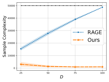
Figure 2: Comparison of Sample Complexity

The runtime of both algorithms are shown in Table 4. RAGE shows clear advantage in runtime and our algorithm suffers from computational overheads of conducting model selection.

Table 4: Comparison of Runtime

$\varepsilon$	$10^{-2}$	$10^{-3}$	$10^{-4}$	$10^{-5}$
RAGE	$85.99\,$s	$144.78\,$s	$249.79\,$s	$357.98\,$s
Ours	$287.09\,$s	$339.67\,$s	$489.50\,$s	$678.93\,$s

We remark that, for the current experiment setups with $d_{\star}$ and $D\in\left\{25,50,75,100\right\}$, our algorithm does not perform well if $\theta_{\star}$ is chosen to be flat, e.g., $\theta_{\star}=[\frac{1}{\sqrt{d_{\star}}},\dots,\frac{1}{\sqrt{d_{\star}}},0,\dots,0]^{\top}\in{\mathbb{R}}^{D}$. However, we believe that one will eventually see model selection gains if $D$ is chosen to be large enough (and allowing each algorithm takes more samples before force-stopped). One may need to overcome the computational burdens, e.g., developing practical (or heuristic-based) implementations of our algorithm and RAGE, before running experiments in higher dimensional spaces. We leave large-scale evaluations for future work.

References

- Alieva et al. (2021) Ayya Alieva, Ashok Cutkosky, and Abhimanyu Das. Robust pure exploration in linear bandits with limited budget. In International Conference on Machine Learning, pages 187–195. PMLR, 2021.
- Allen-Zhu et al. (2020) Zeyuan Allen-Zhu, Yuanzhi Li, Aarti Singh, and Yining Wang. Near-optimal discrete optimization for experimental design: A regret minimization approach. Mathematical Programming, pages 1–40, 2020.
- Audibert et al. (2010) Jean-Yves Audibert, Sébastien Bubeck, and Rémi Munos. Best arm identification in multi-armed bandits. In COLT, pages 41–53. Citeseer, 2010.
- Camilleri et al. (2021) Romain Camilleri, Julian Katz-Samuels, and Kevin Jamieson. High-dimensional experimental design and kernel bandits. arXiv preprint arXiv:2105.05806, 2021.
- Degenne and Koolen (2019) Rémy Degenne and Wouter M Koolen. Pure exploration with multiple correct answers. In Advances in Neural Information Processing Systems, pages 14564–14573, 2019.
- Degenne et al. (2020) Rémy Degenne, Pierre Ménard, Xuedong Shang, and Michal Valko. Gamification of pure exploration for linear bandits. In International Conference on Machine Learning, pages 2432–2442. PMLR, 2020.
- Fiez et al. (2019) Tanner Fiez, Lalit Jain, Kevin G Jamieson, and Lillian Ratliff. Sequential experimental design for transductive linear bandits. In Advances in Neural Information Processing Systems, pages 10666–10676, 2019.
- Foster et al. (2019) Dylan J Foster, Akshay Krishnamurthy, and Haipeng Luo. Model selection for contextual bandits. arXiv preprint arXiv:1906.00531, 2019.
- Hoffman et al. (2014) Matthew Hoffman, Bobak Shahriari, and Nando Freitas. On correlation and budget constraints in model-based bandit optimization with application to automatic machine learning. In Artificial Intelligence and Statistics, pages 365–374. PMLR, 2014.
- Jaggi (2013) Martin Jaggi. Revisiting frank-wolfe: Projection-free sparse convex optimization. In International Conference on Machine Learning, pages 427–435. PMLR, 2013.
- Katz-Samuels and Jamieson (2020) Julian Katz-Samuels and Kevin Jamieson. The true sample complexity of identifying good arms. In International Conference on Artificial Intelligence and Statistics, pages 1781–1791. PMLR, 2020.
- Katz-Samuels et al. (2020) Julian Katz-Samuels, Lalit Jain, Zohar Karnin, and Kevin Jamieson. An empirical process approach to the union bound: Practical algorithms for combinatorial and linear bandits. arXiv preprint arXiv:2006.11685, 2020.
- Kaufmann et al. (2016) Emilie Kaufmann, Olivier Cappé, and Aurélien Garivier. On the complexity of best-arm identification in multi-armed bandit models. The Journal of Machine Learning Research, 17(1):1–42, 2016.
- Kiefer and Wolfowitz (1960) Jack Kiefer and Jacob Wolfowitz. The equivalence of two extremum problems. Canadian Journal of Mathematics, 12:363–366, 1960.
- Lattimore et al. (2020) Tor Lattimore, Csaba Szepesvari, and Gellert Weisz. Learning with good feature representations in bandits and in rl with a generative model. In International Conference on Machine Learning, pages 5662–5670. PMLR, 2020.
- Pacchiano et al. (2020) Aldo Pacchiano, My Phan, Yasin Abbasi-Yadkori, Anup Rao, Julian Zimmert, Tor Lattimore, and Csaba Szepesvari. Model selection in contextual stochastic bandit problems. arXiv preprint arXiv:2003.01704, 2020.
- Pukelsheim (2006) Friedrich Pukelsheim. Optimal design of experiments. SIAM, 2006.
- Shalev-Shwartz and Ben-David (2014) Shai Shalev-Shwartz and Shai Ben-David. Understanding machine learning: From theory to algorithms. Cambridge university press, 2014.
- Soare et al. (2014) Marta Soare, Alessandro Lazaric, and Rémi Munos. Best-arm identification in linear bandits. In Advances in Neural Information Processing Systems, pages 828–836, 2014.
- Stone (1978) M Stone. Cross-validation: A review. Statistics: A Journal of Theoretical and Applied Statistics, 9(1):127–139, 1978.
- Stone (1974) Mervyn Stone. Cross-validatory choice and assessment of statistical predictions. Journal of the Royal Statistical Society: Series B (Methodological), 36(2):111–133, 1974.
- Tao et al. (2018) Chao Tao, Saúl Blanco, and Yuan Zhou. Best arm identification in linear bandits with linear dimension dependency. In International Conference on Machine Learning, pages 4877–4886, 2018.
- Xu et al. (2018) Liyuan Xu, Junya Honda, and Masashi Sugiyama. A fully adaptive algorithm for pure exploration in linear bandits. In International Conference on Artificial Intelligence and Statistics, pages 843–851, 2018.
- Yang and Tan (2021) Junwen Yang and Vincent YF Tan. Towards minimax optimal best arm identification in linear bandits. arXiv preprint arXiv:2105.13017, 2021.
- Zhu and Nowak (2021) Yinglun Zhu and Robert Nowak. Pareto optimal model selection in linear bandits. arXiv preprint arXiv:2102.06593, 2021.
- Zhu et al. (2021) Yinglun Zhu, Dongruo Zhou, Ruoxi Jiang, Quanquan Gu, Rebecca Willett, and Robert Nowak. Pure exploration in kernel and neural bandits. arXiv preprint arXiv:2106.12034, 2021.