Global stability of SAIRS epidemic models

Abstract

We study an SAIRS-type epidemic model with vaccination, where the role of asymptomatic and symptomatic infectious individuals are explicitly considered in the transmission patterns of the disease. We provide a global stability analysis for the model. We determine the value of the basic reproduction number $\mathcal{R}_{0}$ and prove that the disease-free equilibrium is globally asymptotically stable if $\mathcal{R}_{0}<1$ and unstable if $\mathcal{R}_{0}>1$, condition under which a positive endemic equilibrium exists. We investigate the global stability of the endemic equilibrium for some variations of the original model under study and answer to an open problem proposed in Ansumali et al. [1]. In the case of the SAIRS model without vaccination, we prove the global asymptotic stability of the disease-free equilibrium also when $\mathcal{R}_{0}=1$. We provide a thorough numerical exploration of our model, to validate our analytical results.

[inst1]organization=University of Trento, Dept. of Civil, Environmental and Mechanical Engineering,addressline=Via Mesiano, 77, city=Trento, postcode=38123, state=Italy [inst2]organization=TU Delft, Network Architectures and Services Group,addressline=Mekelweg 4, city=Delft, postcode=2628CD, state=The Netherlands [inst3]organization=University of Trento, Dept. of Mathematics,addressline=Via Sommarive 14, city=Povo - Trento, postcode=38123, state=Italy

1 Introduction

The recent Covid-19 pandemic has demonstrated to what extend the study of mathematical models of infectious disease is crucial to provide particularly effective tools to help policy-makers contain the spread of the disease. Many large scale data-driven simulations have been used to examine and forecast aspects of the current epidemic spreading [2, 3], as well as in other past epidemics [4, 5, 6]. However, the study of theoretical effective epidemic models able to catch the salient transmission patterns of an epidemic, but that are yet mathematical tractable, offers essential insight to understand the qualitative behavior of the epidemic, and provides useful information for control policies.

A peculiar, yet crucial feature of the recent Covid-19 pandemic is that “asymptomatic” individuals, despite showing no symptoms, are able to transmit the infection (see e.g., [7, 8, 9, 10], where a considerable fraction of SARS-Cov-2 infections have been attributed to asymptomatic individuals). This is one of the main aspect that has allowed the virus to circulate widely in the population, since asymptomatic cases often remain unidentified, and presumably have more contacts than symptomatic cases, since lack of symptoms often implies a lack of quarantine. Hence, the contribution of the so called “silent spreaders” to the infection transmission dynamics should be considered in mathematical epidemic models [11].

Models that incorporate an asymptomatic compartment already exist in literature [12, 13, 14], but have not been analytically studied as thoroughly as more famous compartmental models. In this work, we consider an SAIRS (Susceptible-Asymptomatic infected-symptomatic Infected-Recovered-Susceptible) model based on the one proposed in [11, Sec. 2], in which the authors provide only a local stability analysis. An SAIR-type model is studied in [1] with application to SARS-CoV-2. After a global stability analysis of the model, the authors present a method to estimate the parameters. They apply the estimation method to Covid-related data from several countries, demonstrating that the predicted epidemic trajectories closely match actual data. The global stability analysis in [1] regards only a simplified version of the model in [11]: first, recovered people do not lose their immunity; moreover, the infection rates of the asymptomatic and symptomatic individuals are equal, as well as their recovery rates, while in [11] these parameters are considered to be potentially different.

Thus, the main scope of our work is to provide a global stability analysis of the model proposed in [11], and for some variations thereof. In addition, we include in our model the possibility of vaccination. In the investigation of global stability, we answer an open problem left in [1]. In particular, we study the global asymptotic stability (GAS) of the disease-free equilibrium (DFE) and provide results related to the global asymptotic stability of the endemic equilibrium (EE) for many variations of the model, as we will explain in detail in Sec. 1.1.

The rigorous proof of global stability, especially for the positive endemic equilibrium, becomes a challenging mathematical problem for many disease models due to their complexity and high dimension [15].

The classical, and most commonly used method for GAS analysis is provided by the Lyapunov stability theorem and LaSalle’s invariance principle. These approaches are successfully applied, for example, to the SIR, SEIR and SIRS models (see, e.g. [16, 17, 15]). Others techniques have appeared in literature, and were successfully applied to global stability arguments for various epidemic models. For example, the Li–Muldowney geometric approach [18, 19] was used to determine the global asymptotic stability of the SEIR and SEIRS models [20, 21, 22], of some epidemic models with bilinear incidence [23], as well as of SIR and SEIR epidemic models with information dependent vaccination [24, 25]. Applications of Li–Muldowney geometric approach can also be found in population dynamics [26].

Unlike the more famous and studied epidemic models, much less attention has been paid to the SAIR(S)-type models. Thus, we think that a deeper understanding of these kind of models is needed, and could prove to be very useful in the epidemiological field. Indeed, in various communicable diseases, such as influenza, cholera, shigella, Covid-19, an understanding of the infection transmission by asymptomatic individuals may be crucial in determining the overall pattern of the epidemic dynamics [13, 27].

In our model, the total population $N$ is partitioned into four compartments, namely $S$, $A$, $I$, $R$, which represent the fraction of Susceptible, Asymptomatic infected, symptomatic Infected and Recovered individuals, respectively, such that $N=S+A+I+R$. The infection can be transmitted to a susceptible through a contact with either an asymptomatic infected individual, at rate $\beta_{A}$, or a symptomatic, at rate $\beta_{I}$. This aspect differentiates an SAIR-type model from the more used and studied SEIR-type model, where once infected a susceptible individual enters an intermediate stage called “Exposed” (E), but a contact between a person in state $E$ and one in state $S$ does not lead to an infection.

In our model instead, once infected, all susceptible individuals enter an asymptomatic state, indicating in any case a delay between infection and symptom onset. We include in the asymptomatic class both individuals who will never develop the symptoms and pre-symptomatic who will eventually become symptomatic. The pre-symptomatic phase seems to have a relevant role in the transmission: for example, in the case of Covid-19, empirical evidence shows that the serial interval tends to be shorter than the incubation period, suggesting that a relevant proportion of secondary transmission can occur prior to symptoms onset [3]; the importance of the pre-symptomatic phase in the transmission is underlined also for other diseases, such as dengue [28], and H1N1 influenza [29].

From the asymptomatic compartment, an individual can either progress to the class of symptomatic infectious $I$, at rate $\alpha$, or recover without ever developing symptoms, at rate $\delta_{A}$. An infected individuals with symptoms can recover at a rate $\delta_{I}$. We assume that the recovered individuals do not obtain a long-life immunity and can return to the susceptible state after an average time $1/\gamma$. We also assume that a proportion $\nu$ of susceptible individuals receive a dose of vaccine which grants them a temporary immunity. We do not add a compartment for the vaccinated individuals, not distinguishing the vaccine-induced immunity from the natural one acquired after recovery from the virus. Moreover, we consider the vital dynamics of the entire population and, for simplicity, we assume that the rate of births and deaths are the same, equal to $\mu$; we do not distinguish between natural deaths and disease related deaths.

1.1 Outline and main results

In Sec. 2, we present the system of equations for the SAIRS model with vaccination, providing its positive invariant set. In Sec. 3, we determine the value of the basic reproduction number $\mathcal{R}_{0}$ and prove that if $\mathcal{R}_{0}<1$, the DFE is GAS.

In Sec. 4, we discuss the uniform persistence of the disease, the existence and uniqueness of the endemic equilibrium, and we investigate its stability properties. In particular, first we provide the local asymptotic stability of the EE, then we investigate its global asymptotic stability for some variations of the original model under study. We start by considering the open problem left in [1], where the global stability of an SAIR model with vital dynamics is studied. The authors consider a disease which confers permanent immunity, meaning that the recovered individuals never return to the susceptible state. Moreover, they impose the restrictions $\beta_{A}=\beta_{I}$ and $\delta_{A}=\delta_{I}$, and leave the global stability of the endemic equilibrium when $\beta_{A}\neq\beta_{I}$ and $\delta_{A}\neq\delta_{I}$, as an open problem. Thus, in Sec. 4.1.1, we directly solve the open problem left in [1], by considering an SAIR model (i.e., $\gamma=0$), with $\beta_{A}\neq\beta_{I}$ and $\delta_{A}\neq\delta_{I}$, including in addition the possibility of vaccination. We consider the basic reproduction number $\mathcal{R}_{0}$ for this model and prove that if $\mathcal{R}_{0}>1$ the EE is GAS. In Sec. 4.1.2, we study the GAS of the EE for an SAIRS model (i.e., $\gamma\neq 0$) with vaccination, with the restrictions $\beta_{A}=\beta_{I}$ and $\delta_{A}=\delta_{I}$, proving that if $\mathcal{R}_{0}>1$ the EE is GAS. In Sec. 4.1.3, we investigate the global stability of the SAIRS model, where $\beta_{A}\neq\beta_{I}$ and $\delta_{A}\neq\delta_{I}$, i.e., the model proposed in [11], with in addition the possibility of vaccination. In this case, we use a geometric approach to global stability for nonlinear autonomous systems due to Lu and Lu [30], that generalizes the criteria developed by Li and Muldowney [18, 19]. We prove that if $\mathcal{R}_{0}>1$ and $\beta_{A}<\delta_{I}$, the EE is GAS.

In Sec. 4.2, we are able to prove the GAS of the DFE also in the case $\mathcal{R}_{0}=1$, assuming that no vaccination campaign is in place. In Sec. 5, we validate our analytical results via several numerical simulations and deeper explore the role of parameters.

2 The SAIRS model with vaccination

We consider an extension of the SAIRS model presented in [11]. The system of ODEs which describes the model is given by

$$\begin{split}\frac{dS(t)}{dt}&=\mu-\bigg{(}\beta_{A}A(t)+\beta_{I}I(t)\bigg{)}S(t)-(\mu+\nu)S(t)+\gamma R(t),\\ \frac{dA(t)}{dt}&=\bigg{(}\beta_{A}A(t)+\beta_{I}I(t)\bigg{)}S(t)-(\alpha+\delta_{A}+\mu)A(t),\\ \frac{dI(t)}{dt}&=\alpha A(t)-(\delta_{I}+\mu)I(t),\\ \frac{dR(t)}{dt}&=\delta_{A}A(t)+\delta_{I}I(t)+\nu S(t)-(\gamma+\mu)R(t),\end{split}$$ (1)

with initial condition $(S(0),A(0),I(0),R(0))$ belonging to the set

$$\bar{\Gamma}=\{(S,A,I,R)\in\mathbb{R}_{+}^{4}|S+A+I+R=1\},$$ (2)

where $\mathbb{R}_{+}^{4}$ is the non-negative orthant of $\mathbb{R}^{4}$. The flow diagram for system (1) is given in Figure 1.

Figure 1: Flow diagram for system (1).

Assuming initial conditions in $\bar{\Gamma}$, $S(t)+A(t)+I(t)+R(t)=1,$ for all $t\geq 0$; hence, system (1) is equivalent to the following three-dimensional dynamical system

$$\begin{split}\frac{dS(t)}{dt}&=\mu-\bigg{(}\beta_{A}A(t)+\beta_{I}I(t)\bigg{)}S(t)-(\mu+\nu+\gamma)S(t)+\gamma(1-A(t)-I(t)),\\ \frac{dA(t)}{dt}&=\bigg{(}\beta_{A}A(t)+\beta_{I}I(t)\bigg{)}S(t)-(\alpha+\delta_{A}+\mu)A(t),\\ \frac{dI(t)}{dt}&=\alpha A(t)-(\delta_{I}+\mu)I(t),\end{split}$$ (3)

with initial condition $(S(0),A(0),I(0))$ belonging to the set

$$\Gamma=\{(S,A,I)\in\mathbb{R}_{+}^{3}|S+A+I\leq 1\}.$$

System (3) can be written in vector notation as

$$\frac{dx(t)}{dt}=f(x(t)),$$

where $x(t)=(S(t),A(t),I(t))$ and $f(x(t))=(f_{1}(x(t)),f_{2}(x(t)),f_{3}(x(t)))$ is defined according to (3).

Theorem 1.

$\Gamma$ is positively invariant for system (3). That is, for all initial values $x(0)\in\Gamma$, the solution $x(t)$ of (3) will remain in $\Gamma$ for all $t>0$.

Proof.

A compact set $C$ is invariant for the system $dx(t)/dt=f(x(t))$ if at each point $y\in\partial\Delta$ (the boundary of $C$), the vector $f(y)$ is tangent or pointing into the set [31].

The boundary $\partial\Gamma$ consists of the following $4$ hyperplanes:

$$H_{1} =\{(S,A,I)\in\Gamma\;|\;S=0\},\qquad H_{2}=\{((S,A,I)\in\Gamma\;|\;A=0\},$$

$$H_{3} =\{(S,A,I)\in\Gamma\;|\;I=0\},\quad H_{4}=\{(S,A,I)\in\Gamma\;|\;S+A+I=1\}$$

whose respective outer normal vectors are:

$$\eta_{1}=(-1,0,0),\qquad\eta_{2}=(0,-1,0),\qquad\eta_{3}=(0,0,-1),\qquad\eta_{4}=(1,1,1).$$

Thus, let us consider a point $x\in\partial\Gamma$. To prove the statement, we distinguish among four cases.

Case 1: $S=0$. Then, since $A+I\leq 1$

$$\langle f(x),\eta_{1}\rangle=-\mu-\gamma(1-A-I)\leq 0.$$

Case 2: $A=0$. Then, since $S\geq 0$, $I\geq 0$

$$\langle f(x),\eta_{2}\rangle=-\beta_{I}IS\leq 0.$$

Case 3: $I=0$. Then, since $A\geq 0$

$$\langle f(x),\eta_{3}\rangle=-\alpha A\leq 0.$$

Case 4: $S+A+I=1$. Then, since $S\geq 0$, $A\geq 0$, $I\geq 0$

$$\langle f(x),\eta_{4}\rangle=-\nu S-\delta_{A}A-\delta_{I}I\leq 0.$$

Thus, any solution that starts in $\partial\Gamma$ will remain inside $\Gamma$.     

3 Extinction

In this section, we provide the value of the basic reproduction number, that is defined as the expected number of secondary infections produced by an index case in a completely susceptible population [32, 33]. This numerical value gives a measure of the potential for disease spread within a population [34]. Then, we investigate the stability properties of the disease-free equilibrium of the system (3), that is equal to

$$x_{0}=\left(S_{0},A_{0},I_{0}\right)=\left(\frac{\mu+\gamma}{\mu+\nu+\gamma},0,0\right).$$ (4)

Lemma 2.

The basic reproduction number $\mathcal{R}_{0}$ of (3) is given by

$$\mathcal{R}_{0}=\left(\beta_{A}+\dfrac{\alpha\beta_{I}}{\delta_{I}+\mu}\right)\dfrac{\gamma+\mu}{(\alpha+\delta_{A}+\mu)(\nu+\gamma+\mu)}.$$ (5)

Proof.

Let us use the next generation matrix method [35] to find $\mathcal{R}_{0}$. System (3) has 2 disease compartments, denoted by $A$ and $I$. We can write

$$\frac{dA(t)}{dt} =\mathcal{F}_{1}(S(t),A(t),I(t))-\mathcal{V}_{1}(S(t),A(t),I(t)),$$

$$\frac{dI(t)}{dt} =\mathcal{F}_{2}(S(t),A(t),I(t))-\mathcal{V}_{2}(S(t),A(t),I(t)),$$

where

$$\mathcal{F}_{1}(S(t),A(t),I(t))=\bigg{(}\beta_{A}A(t)+\beta_{I}I(t)\bigg{)}S(t),\qquad\mathcal{V}_{1}(S(t),A(t),I(t))=(\alpha+\delta_{A}+\mu)A(t),$$

$$\mathcal{F}_{2}(S(t),A(t),I(t))=0,\qquad\mathcal{V}_{2}(S(t),A(t),I(t))=-\alpha A(t)+(\delta_{I}+\mu)I(t).$$

Thus, we obtain

$$F=\left(\begin{matrix}\dfrac{\partial\mathcal{F}_{1}}{\partial A}(x_{0})&\dfrac{\partial\mathcal{F}_{1}}{\partial I}(x_{0})\\ \\ \dfrac{\partial\mathcal{F}_{2}}{\partial A}(x_{0})&\dfrac{\partial\mathcal{F}_{2}}{\partial I}(x_{0})\end{matrix}\right)=\left(\begin{matrix}\beta_{A}S_{0}&\beta_{I}S_{0}\\ 0&0\end{matrix}\right),\qquad\text{where }S_{0}=\dfrac{\gamma+\mu}{\gamma+\mu+\nu},$$ (6)

$$V=\left(\begin{matrix}\dfrac{\partial\mathcal{V}_{1}}{\partial A}(x_{0})&\dfrac{\partial\mathcal{V}_{1}}{\partial I}(x_{0})\\ \\ \dfrac{\partial\mathcal{V}_{2}}{\partial A}(x_{0})&\dfrac{\partial\mathcal{V}_{2}}{\partial I}(x_{0})\end{matrix}\right)=\left(\begin{matrix}\alpha+\delta_{A}+\mu&0\\ -\alpha&\delta_{I}+\mu\end{matrix}\right),$$ (7)

from which

$$V^{-1}=\left(\begin{matrix}\dfrac{1}{\alpha+\delta_{A}+\mu}&0\\ \\ \dfrac{\alpha}{(\alpha+\delta_{A}+\mu)(\delta_{I}+\mu)}&\dfrac{1}{\delta_{I}+\mu}\end{matrix}\right).$$

The next generation matrix is defined as $M:=FV^{-1}$, that is

$$M=\left(\begin{matrix}\dfrac{\beta_{A}S_{0}}{\alpha+\delta_{A}+\mu}+\dfrac{\alpha\beta_{I}S_{0}}{(\alpha+\delta_{A}+\mu)(\delta_{I}+\mu)}&\dfrac{\beta_{I}S_{0}}{\delta_{I}+\mu}\\ \\ 0&0\end{matrix}\right).$$

The basic reproduction number $\mathcal{R}_{0}$ is defined as the spectral radius of $M$, denoted by $\rho(M)$. Thus, with a direct computation, we obtain (5).     

In the following, we recall some results that we will use to prove the global asymptotic stability of the disease-free equilibrium $x_{0}$ of (3).

Lemma 3.

The matrix $(F-V)$ has a real spectrum. Moreover, if $\rho(FV^{-1})<1$, all the eigenvalues of $(F-V)$ are negative.

Proof.

From (6) and (7)

$$(F-V)=\left(\begin{matrix}\beta_{A}S_{0}-(\alpha+\delta_{A}+\mu)&\beta_{I}S_{0}\\ \alpha&-(\delta_{I}+\mu)\end{matrix}\right).$$ (8)

Since $(F-V)$ is a $2\times 2$ matrix whose off-diagonal elements have the same sign, it is easy to see that its eigenvalues are real. Indeed, for a generic matrix $A=\left(\begin{matrix}a&b\\ c&d\end{matrix}\right)$ with $\text{sign}(b)=\text{sign}(c)$, the eigenvalues can be easily shown to be real by explicitly computing them:

$$\lambda_{1,2}=\dfrac{(a+d)\pm\sqrt{(a-d)^{2}+4bc}}{2},$$

and noticing that the radicand is the sum of two non-negative values. Now, if $\rho(FV^{-1})=\mathcal{R}_{0}<1$ all eigenvalues of $(F-V)$ are negative as a consequence of [34, Lemma 2].     

Theorem 4.

The disease-free equilibrium $x_{0}$ of (3) is locally asymptotically stable if $\mathcal{R}_{0}<1$, and unstable if $\mathcal{R}_{0}>1$.

Proof.

See [34, Theorem 1].     

Theorem 5.

The disease-free equilibrium $x_{0}$ of (3) is globally asymptotically stable if $\mathcal{R}_{0}<1$.

Proof.

Since $\Gamma$ is an invariant set for (3) and in view of Theorem 4, it is sufficient to show that for all $x(0)\in\Gamma$

$$\lim_{t\to\infty}A(t)=0,\qquad\lim_{t\to\infty}I(t)=0,\qquad\text{and}\qquad\lim_{t\to\infty}S(t)=S_{0},$$

with $S_{0}$ as in (4). From the first equation of (3) follows that

$$\frac{dS(t)}{dt}\leq\mu+\gamma-(\mu+\nu+\gamma)S(t).$$

It easy to see that $S_{0}$ is a global asymptotically stable equilibrium for the comparison equation

$$\frac{dy(t)}{dt}=\mu+\gamma-(\mu+\nu+\gamma)y(t).$$

Then, for any $\varepsilon>0$, there exists $\bar{t}>0$, such that for all $t\geq\bar{t}$, it holds

$$S(t)\leq S_{0}+\varepsilon,$$ (9)

hence

$$\limsup_{t\to\infty}S(t)\leq S_{0}.$$ (10)

Now, from (9) and second and third equation of (3), we have that for $t\geq\bar{t}$

$$\frac{dA(t)}{dt} \leq\bigg{(}\beta_{A}A(t)+\beta_{I}I(t)\bigg{)}(S_{0}+\varepsilon)-(\alpha+\delta_{A}+\mu)A(t),$$

$$\frac{dI(t)}{dt} =\alpha A(t)-(\delta_{I}+\mu)I(t).$$

Let us now consider the comparison system

$$\frac{dw_{1}(t)}{dt} =\bigg{(}\beta_{A}w_{1}(t)+\beta_{I}w_{2}(t)\bigg{)}(S_{0}+\varepsilon)-(\alpha+\delta_{A}+\mu)w_{1}(t),$$

$$\frac{dw_{2}(t)}{dt} =\alpha w_{1}(t)-(\delta_{I}+\mu)w_{2}(t),\qquad w_{1}(\bar{t})=A(\bar{t}),\quad w_{2}(\bar{t})=I(\bar{t}),$$

that we can rewrite as

$$\frac{dw(t)}{dt}=(F_{\varepsilon}-V_{\varepsilon})w(t),$$

where $w(t)=(w_{1}(t),w_{2}(t))^{T}$ and $F_{\varepsilon}-V_{\varepsilon}$ is the matrix in (8), computed in $x_{0}(\varepsilon)=(S_{0}+\varepsilon,0,0)$. Let us note that if $\mathcal{R}_{0}=\rho(FV^{-1})<1$, we can choose a sufficient small $\varepsilon>0$ such that $\rho(F_{\varepsilon}V_{\varepsilon}^{-1})<1$. Then, by applying Lemma 3 to $(F_{\varepsilon}-V_{\varepsilon})$, we obtain that it has a real spectrum and all its eigenvalues are negative. It follows that $\lim_{t\to\infty}w(t)=0$ , whatever the initial conditions are (see, e.g., [36]), from which

$$\lim_{t\to\infty}A(t)=0,\qquad\text{and}\qquad\lim_{t\to\infty}I(t)=0.$$

Now, for any $\varepsilon>0$ there exists $\bar{t}_{1}$ such that for any $t>\bar{t}_{1}$, $I(t)<\varepsilon$ and $A(t)<\varepsilon$. So, for $t>\bar{t}_{1}$ we have

$$\frac{dS(t)}{dt}\geq\mu-\varepsilon(\beta_{A}+\beta_{I})S(t)-(\mu+\nu+\gamma)S(t)+\gamma(1-2\varepsilon).$$

It easy to see that $\frac{\mu+\gamma(1-2\varepsilon)}{\varepsilon(\beta_{A}+\beta_{I})+(\mu+\nu+\gamma)}$ is a global asymptotically stable equilibrium for the comparison equation

$$\frac{dy(t)}{dt}=\mu-\varepsilon(\beta_{A}+\beta_{I})y(t)-(\mu+\nu+\gamma)y(t)+\gamma(1-2\varepsilon).$$

Thus, for any $\zeta>0$, there exists $\bar{t}_{2}>0$ such that for all $t\geq\bar{t}_{2}$,

$$S(t)\geq\frac{\mu+\gamma(1-2\varepsilon)}{\varepsilon(\beta_{A}+\beta_{I})+(\mu+\nu+\gamma)}-\zeta.$$

Then, for any $\varepsilon>0$, we have

$$\liminf_{t\to\infty}S(t)\geq\frac{\mu+\gamma(1-2\varepsilon)}{\varepsilon(\beta_{A}+\beta_{I})+(\mu+\nu+\gamma)}.$$

Letting $\varepsilon$ go to $0$, we have $\liminf_{t\to\infty}S(t)\geq S_{0}$, that combined with (10) gives us

$$\lim_{t\to\infty}S(t)=S_{0}.$$

    

4 Global stability of the endemic equilibrium

In this section, we discuss the uniform persistence of the disease, the existence and uniqueness of an endemic equilibrium, and we investigate its stability properties.

We say that the disease is endemic if both the asymptomatic and infected fractions in the population remains above a certain positive level for a sufficiently large time. The notion of uniform persistent can be used to represent and analyze the endemic scenario [20]. In the following, with the notation $\mathring{\Theta}$, we indicate the interior of a set $\Theta$.

Definition 6.

System (3) is said to be uniformly persistent if there exists a constant $0<\varepsilon<1$ such that any solution $x(t)=(S(t),A(t),I(t))$ with $x(0)\in\mathring{\Gamma}$ satisfies

$$\min\{\liminf_{t\to\infty}S(t),\quad\liminf_{t\to\infty}A(t),\quad\liminf_{t\to\infty}I(t)\}\geq\varepsilon.$$ (11)

To address the uniform persistence of our system, we need the following result.

Lemma 7.

The DFE $x_{0}$ is the unique equilibrium of (3) on $\partial\Gamma$.

Proof.

Let us assume that $\bar{x}=(\bar{S},\bar{A},\bar{I})$ is an equilibrium of (3) on $\partial\Gamma$. Then, there are three possibilities:

Case 1: $\bar{S}=0$. It follows from the second equation of (3) that $\bar{A}=0$ and, consequently, from the third equation that $\bar{I}=0$. Then, from the first equation of (3) we have $\gamma(\bar{A}+\bar{I})={\mu+\gamma}>0$, and a contradiction occurs.

Case 2: $\bar{A}=0$. It follows from the third equation of (3) that $\bar{I}=0$, and from the first that $\bar{S}=S_{0}$.

Case 3: $\bar{I}=0$. Analogously to Case 2, we find that $\bar{A}=0$ and $\bar{S}=S_{0}$.

Case 4: $\bar{S}+\bar{A}+\bar{I}=1$. By summing the equations in (3), we have $\delta_{A}\bar{A}+\delta_{I}\bar{I}+\nu\bar{S}=0$, a contradiction.

By combining the above discussions the statement follows.     

Theorem 8.

If $\mathcal{R}_{0}>1$, system (3) is uniformly persistent and there exists at least one endemic equilibrium in $\mathring{\Gamma}$.

Proof.

By Lemma 7, the largest invariant set on $\partial\Gamma$ is the singleton $\{x_{0}\}$, which is isolated. If $\mathcal{R}_{0}>1$, we know from Theorem 4 that $x_{0}$ is unstable. Then, by using [37, Thm 20], and similar arguments in [20, Prop. 3.3], we can assert that the instability of $x_{0}$ implies the uniform persistence of (3). The uniform persistence and the positive invariance of the compact set $\Gamma$ imply the existence of an endemic equilibrium in $\mathring{\Gamma}$ (see, e.g., [38, Thm 2.8.6] or [15, Thm. 2.2]).     

Lemma 9.

There exists an endemic equilibrium $x^{*}=(S^{*},A^{*},I^{*})$ in $\mathring{\Gamma}$ for system (3) if and only if $\mathcal{R}_{0}>1$. Furthermore, this equilibrium is unique.

Proof.

Let us consider (3); we equate the right hand sides to 0, and assume $A^{*},I^{*}\neq 0$. From the third equation we obtain

$$A^{*}=\dfrac{\delta_{I}+\mu}{\alpha}I^{*},$$ (12)

and replacing it in the second equation

$$\left(\beta_{A}\dfrac{\delta_{I}+\mu}{\alpha}+\beta_{I}\right)I^{*}S^{*}-(\alpha+\delta_{A}+\mu)\dfrac{\delta_{I}+\mu}{\alpha}I^{*}=0.$$

Since $I^{*}\neq 0$, it follows that

$$S^{*}=\dfrac{(\alpha+\delta_{A}+\mu)(\delta_{I}+\mu)}{\beta_{A}(\delta_{I}+\mu)+\beta_{I}\alpha}.$$ (13)

Let us substitute the expressions (12) and (13) in the first equation, then we obtain

$$\mu-\left(\beta_{A}\dfrac{\delta_{I}+\mu}{\alpha}+\beta_{I}\right)\dfrac{(\alpha+\delta_{A}+\mu)(\delta_{I}+\mu)}{\beta_{A}(\delta_{I}+\mu)+\beta_{I}\alpha}I^{*}-(\mu+\nu+\gamma)\dfrac{(\alpha+\delta_{A}+\mu)(\delta_{I}+\mu)}{\beta_{A}(\delta_{I}+\mu)+\beta_{I}\alpha}+\gamma\left(1-\dfrac{\delta_{I}+\mu}{\alpha}I^{*}-I^{*}\right)=0,$$

which implies that

$$I^{*} =\dfrac{\mu-(\mu+\nu+\gamma)\dfrac{(\alpha+\delta_{A}+\mu)(\delta_{I}+\mu)}{\beta_{A}(\delta_{I}+\mu)+\beta_{I}\alpha}+\gamma}{\dfrac{1}{\alpha}(\beta_{A}(\delta_{I}+\mu)+\beta_{I}\alpha)\dfrac{(\alpha+\delta_{A}+\mu)(\delta_{I}+\mu)}{\beta_{A}(\delta_{I}+\mu)+\beta_{I}\alpha}+\gamma\dfrac{\delta_{I}+\mu}{\alpha}+\gamma}$$

$$=\dfrac{(\mu+\gamma)(\beta_{A}(\delta_{I}+\mu)+\beta_{I}\alpha)-(\mu+\nu+\gamma)(\alpha+\delta_{A}+\mu)(\delta_{I}+\mu)}{\dfrac{\beta_{A}(\delta_{I}+\mu)+\beta_{I}\alpha}{\alpha}\left((\alpha+\delta_{A}+\mu+\gamma)(\delta_{I}+\mu)+\gamma\alpha\right)}$$

$$=\dfrac{(\delta_{I}+\mu)\left((\mu+\gamma)\left(\beta_{A}+\beta_{I}\dfrac{\alpha}{\delta_{I}+\mu}\right)-(\mu+\nu+\gamma)(\alpha+\delta_{A}+\mu)\right)}{\dfrac{\beta_{A}(\delta_{I}+\mu)+\beta_{I}\alpha}{\alpha}\left((\alpha+\delta_{A}+\mu+\gamma)(\delta_{I}+\mu)+\gamma\alpha\right)}$$

$$=\dfrac{(\delta_{I}+\mu)(\mu+\nu+\gamma)(\alpha+\delta_{A}+\mu)\left(\dfrac{(\mu+\gamma)}{(\mu+\nu+\gamma)(\alpha+\delta_{A}+\mu)}\left(\beta_{A}+\beta_{I}\dfrac{\alpha}{\delta_{I}+\mu}\right)-1\right)}{\dfrac{\beta_{A}(\delta_{I}+\mu)+\beta_{I}\alpha}{\alpha}\left((\alpha+\delta_{A}+\mu+\gamma)(\delta_{I}+\mu)+\gamma\alpha\right)}$$

$$=\dfrac{\alpha(\delta_{I}+\mu)(\mu+\nu+\gamma)(\alpha+\delta_{A}+\mu)}{(\beta_{A}(\delta_{I}+\mu)+\beta_{I}\alpha)\left((\alpha+\delta_{A}+\mu+\gamma)(\delta_{I}+\mu)+\gamma\alpha\right)}(\mathcal{R}_{0}-1).$$ (14)

The endemic equilibrium in $\mathring{\Gamma}$ exists if $A^{*}>0$ and $I^{*}>0$. We obtain that $I^{*}>0$, and consequently $A^{*}>0$, if and only if $\mathcal{R}_{0}-1>0$.     

Theorem 10.

The endemic equilibrium $x^{*}=(S^{*},A^{*},I^{*})$ is locally asymptotically stable in $\mathring{\Gamma}$ for system (3) if $\mathcal{R}_{0}>1$.

Proof.

Note that the expression of (13) and (4) may be written as function of $\mathcal{R}_{0}$; using the expression found in (5), we obtain

$$S^{*}= \dfrac{h_{4}}{\mathcal{R}_{0}},$$ (15)

$$I^{*}= \dfrac{\alpha h_{0}h_{1}h_{2}(\mathcal{R}_{0}-1)}{h_{3}(\beta_{A}h_{2}+\beta_{I}\alpha)},$$ (16)

where we have set $h_{0}=\mu+\nu+\gamma$, $h_{1}=\alpha+\delta_{A}+\mu$, $h_{2}=\delta_{I}+\mu$, $h_{3}=\gamma\alpha+(h_{1}+\gamma)h_{2}$, $h_{4}=\dfrac{\gamma+\mu}{h_{0}}{\leq}1$. Moreover, we can compute

$$\beta_{A}A^{*}+\beta_{I}I^{*}=\dfrac{\beta_{A}h_{2}+\beta_{I}\alpha}{\alpha}I^{*}=\dfrac{h_{0}h_{1}h_{2}(\mathcal{R}_{0}-1)}{h_{3}}.$$ (17)

To determine the stability of the endemic equilibrium $x^{*}$, we need to compute the Jacobian matrix of (3) evaluated in $x^{*}$, that is

$$J_{|x^{*}}=\left(\begin{matrix}-\dfrac{h_{0}h_{1}h_{2}(\mathcal{R}_{0}-1)}{h_{3}}-h_{0}&-\dfrac{\beta_{A}h_{4}}{\mathcal{R}_{0}}-\gamma&-\dfrac{\beta_{I}h_{4}}{\mathcal{R}_{0}}-\gamma\\ \dfrac{h_{0}h_{1}h_{2}(\mathcal{R}_{0}-1)}{h_{3}}&\dfrac{\beta_{A}h_{4}}{\mathcal{R}_{0}}-h_{1}&\dfrac{\beta_{I}h_{4}}{\mathcal{R}_{0}}\\ 0&\alpha&-h_{2}\end{matrix}\right),$$

where we have used (15-17). With the same arguments as in [11, Sec. 2.1], we can conclude that $x^{*}$ is locally asymptotically stable if $\mathcal{R}_{0}>1$.     

4.1 Global Stability

4.1.1 Global stability of the endemic equilibrium in the SAIR model.

In this section, we focus on the global asymptotic stability of the endemic equilibrium of the SAIR model, i.e., system (3) with $\gamma=0$, representing a disease which confers permanent immunity. Here, we answer directly to the open problem left in [1]. Let us note that in our model we have in addition, with respect to the model proposed in [1], the possibility of vaccination.
The dynamic of an SAIR model of this type is described by the following system of equations:

$$\frac{dS(t)}{dt} =\mu-\bigg{(}\beta_{A}A(t)+\beta_{I}I(t)\bigg{)}S(t)-(\mu+\nu)S(t),$$ (18)

$$\frac{dA(t)}{dt} =\bigg{(}\beta_{A}A(t)+\beta_{I}I(t)\bigg{)}S(t)-(\alpha+\delta_{A}+\mu)A(t),$$

$$\frac{dI(t)}{dt} =\alpha A(t)-(\delta_{I}+\mu)I(t),$$

The basic reproduction number is

$${\mathcal{R}_{0}}=\left(\beta_{A}+\dfrac{\alpha\beta_{I}}{\delta_{I}+\mu}\right)\dfrac{\mu}{(\alpha+\delta_{A}+\mu)(\nu+\mu)}.$$

The endemic equilibrium $x^{*}=(S^{*},A^{*},I^{*})$ satisfies the equation

$$\mu =\bigg{(}\beta_{A}A^{*}+\beta_{I}I^{*}\bigg{)}S^{*}+(\mu+\nu)S^{*},$$ (19)

$$(\alpha+\delta_{A}+\mu)A^{*} =\bigg{(}\beta_{A}A^{*}+\beta_{I}(r)I^{*}\bigg{)}S^{*},$$ (20)

$$\alpha A^{*} =(\delta_{I}+\mu)I^{*}.$$ (21)

Theorem 11.

The endemic equilibrium $x^{*}=(S^{*},A^{*},I^{*})$ of (18) is globally asymptotically stable in $\mathring{\Gamma}$ if $\mathcal{R}_{0}>1$.

Proof.

For ease of notation, we will omit the dependence on $t$. Let us consider $c_{1},c_{2}>0$ and the function

$$V=c_{1}V_{1}+c_{2}V_{2}+V_{3},$$

where

$$V_{1}=S^{*}\cdot g\left(\frac{S}{S^{*}}\right),\qquad V_{2}=A^{*}\cdot g\left(\frac{A}{A^{*}}\right),\qquad V_{3}=I^{*}\cdot g\left(\frac{I}{I^{*}}\right),$$

and $g(x)=x-1-\ln x\geq g(1)=0$, for any $x>0$. Let us introduce the notation

$$u=\frac{S}{S^{*}},\qquad y=\frac{A}{A^{*}},\qquad z=\frac{I}{I^{*}}.$$

Differentiating $V$ along the solutions of (18), and using (19), (20), (21), we have

$$\begin{split}c_{1}\frac{dV_{1}}{dt}=&c_{1}\left(1-\frac{S^{*}}{S}\right)\bigg{[}\mu-(\beta_{A}A+\beta_{I}I)S-(\mu+\nu)S\bigg{]}\\ &=c_{1}\left(1-\frac{S^{*}}{S}\right)\bigg{[}-(\mu+\nu)(S-S^{*})-\beta_{A}(AS-A^{*}S^{*})-\beta_{I}(IS-I^{*}S^{*})\bigg{]}\\ &=c_{1}\left(1-\frac{1}{u}\right)\bigg{[}-(\mu+\nu)S^{*}(u-1)-\beta_{A}A^{*}S^{*}(uy-1)-\beta_{I}I^{*}S^{*}(uz-1)\bigg{]},\end{split}$$ (22)

$$\begin{split}c_{2}\frac{dV_{2}}{dt}=&c_{2}\left(1-\frac{A^{*}}{A}\right)\bigg{[}(\beta_{A}A+\beta_{I}I)S-(\alpha+\delta_{A}+\mu)A\bigg{]}\\ &=c_{2}\left(1-\frac{1}{y}\right)\bigg{[}\beta_{A}A^{*}S^{*}uy+\beta_{I}I^{*}S^{*}uz-(\beta_{A}A^{*}+\beta_{I}I^{*})S^{*}y\bigg{]}\\ &=c_{2}\left(1-\frac{1}{y}\right)\bigg{[}\beta_{A}A^{*}S^{*}(uy-y)+\beta_{I}I^{*}S^{*}(uz-y)\bigg{]},\end{split}$$ (23)

$$\begin{split}\frac{dV_{3}}{dt}=&\left(1-\frac{I^{*}}{I}\right)\bigg{[}\alpha A-(\delta_{I}+\mu)I\bigg{]}=\left(1-\frac{I^{*}}{I}\right)\bigg{(}\alpha A-\frac{\alpha IA^{*}}{I^{*}}\bigg{)}\\ &=\alpha A^{*}\bigg{(}1+\frac{A}{A^{*}}-\frac{I}{I^{*}}-\frac{AI^{*}}{A^{*}I}\bigg{)}\\ &\leq\alpha A^{*}\bigg{(}-\ln y+y-z+\ln z\bigg{)}\\ &=\alpha A^{*}(g(y)-g(z)),\end{split}$$ (24)

where we have used the inequality $1-y/z\leq-\ln(y/z)$. Thus, from (22),(23), and (24),

$$\begin{split}\frac{dV}{dt}=&-c_{1}\left(1-\frac{1}{u}\right)(\mu+\nu)S^{*}(u-1)+c_{1}\beta_{A}A^{*}S^{*}\bigg{[}\left(1-\frac{1}{u}\right)(1-uy)+\frac{c_{2}}{c_{1}}\left(1-\frac{1}{y}\right)(uy-y)\bigg{]}\\ &+c_{1}\beta_{I}I^{*}S^{*}\bigg{[}\left(1-\frac{1}{u}\right)(1-uz)+\frac{c_{2}}{c_{1}}\left(1-\frac{1}{y}\right)(uz-y)\bigg{]}+\alpha A^{*}(g(y)-g(z)).\end{split}$$ (25)

Now, for the second and third term in (25), we have

$$\begin{split}&\left(1-\frac{1}{u}\right)(1-uy)+\frac{c_{2}}{c_{1}}\left(1-\frac{1}{y}\right)(uy-y)\\ &=\left(1+\frac{c_{2}}{c_{1}}\right)-\frac{1}{u}-uy\left(1-\frac{c_{2}}{c_{1}}\right)+y\left(1-\frac{c_{2}}{c_{1}}\right)-\frac{c_{2}}{c_{1}}u\\ &=-g\left(\frac{1}{u}\right)-g\left(uy\right)\left(1-\frac{c_{2}}{c_{1}}\right)+\left(g(y)\left(1-\frac{c_{2}}{c_{1}}\right)-g(u)\right),\end{split}$$ (26)

and

$$\begin{split}&\left(1-\frac{1}{u}\right)(1-uz)+\frac{c_{2}}{c_{1}}\left(1-\frac{1}{y}\right)(uz-y)\\ &=\left(1+\frac{c_{2}}{c_{1}}\right)-\frac{1}{u}+z-uz\left(1-\frac{c_{2}}{c_{1}}\right)-\frac{c_{2}}{c_{1}}y-\frac{c_{2}}{c_{1}}\frac{uz}{y}\\ =&-g\left(\frac{1}{u}\right)-\frac{c_{2}}{c_{1}}g\left(\frac{uz}{y}\right)+\left(g(z)-\frac{c_{2}}{c_{1}}g(y)\right)-uz\left(1-\frac{c_{2}}{c_{1}}\right).\end{split}$$ (27)

Thus, substituting (26) and (27) in (25), we obtain

$$\begin{split}\frac{dV}{dt}=&-c_{1}\left(1-\frac{1}{u}\right)(\mu+\nu)S^{*}(u-1)\\ &-c_{1}\beta_{A}A^{*}S^{*}\bigg{[}g\left(\frac{1}{u}\right)+g(uy)\left(1-\frac{c_{2}}{c_{1}}\right)\bigg{]}+c_{1}\beta_{A}A^{*}S^{*}\bigg{[}g(y)\left(1-\frac{c_{2}}{c_{1}}\right)-g(u)\bigg{]}\\ &-c_{1}\beta_{I}I^{*}S^{*}\bigg{[}g\left(\frac{1}{u}\right)+\frac{c_{2}}{c_{1}}g\left(\frac{uz}{y}\right)\bigg{]}+c_{1}\beta_{I}I^{*}S^{*}\bigg{[}g(z)-\frac{c_{2}}{c_{1}}g(y)-uz\left(1-\frac{c_{2}}{c_{1}}\right)\bigg{]}\\ &+\alpha A^{*}(g(y)-g(z)).\end{split}$$

Now, by taking $c_{1}=c_{2}=\frac{\alpha A^{*}}{\beta_{I}I^{*}S^{*}}$, we have

$$\frac{dV}{dt}= -c_{1}\frac{(u-1)^{2}}{u}(\mu+\nu)S^{*}-c_{1}\beta_{A}A^{*}S^{*}\bigg{(}g\left(\frac{1}{u}\right)+g(u)\bigg{)}$$

$$-c_{1}\beta_{I}I^{*}S^{*}\bigg{(}g\left(\frac{1}{u}\right)+g\left(\frac{uz}{y}\right)\bigg{)}.$$

Hence, $\frac{dV}{dt}\leq 0$. Moreover, the set where $\frac{dV}{dt}=0$ is $Z=\{(S,A,I):S=S^{*},I=\frac{AI^{*}}{A^{*}}\},$ and the only compact invariant subset of $Z$ is the singleton $\{x^{*}\}$. The claim follows by LaSalle’s Invariance Principle [39].     

4.1.2 Global stability of the SAIRS model when $\beta_{A}=\beta_{I}:=\beta$ and $\delta_{A}=\delta_{I}:=\delta$

In this case, from (5), the expression of the basic reproduction number becomes

$$\mathcal{R}_{0}=\frac{\beta(\gamma+\mu)}{(\delta+\mu)(\nu+\gamma+\mu)}.$$

Theorem 12.

Let us assume that $\beta_{A}=\beta_{I}=:\beta$ and $\delta_{A}=\delta_{I}=:\delta$. The endemic equilibrium $x^{*}=(S^{*},A^{*},I^{*})$ is globally asymptotically stable in $\mathring{\Gamma}$ for system (3) if $\mathcal{R}_{0}>1$.

Proof.

Let us define $M(t):=A(t)+I(t)$, for all $t\geq 0$. Then, we can rewrite (3) as

$$\frac{dS(t)}{dt} =\mu-\beta M(t)S(t)-(\mu+\nu+\gamma)S(t)+\gamma(1-M(t)),$$

$$\frac{dM(t)}{dt} =\beta M(t)S(t)-(\delta+\mu)M(t).$$

At the equilibrium it holds that

$$\mu+\gamma =\beta M^{*}S^{*}+(\mu+\nu+\gamma)S^{*}+\gamma M^{*},$$ (28)

$$\delta+\mu =\beta S^{*},$$ (29)

where $M^{*}=A^{*}+I^{*}$. In the following, for ease of notation, we will omit the dependence on $t$. Consider the following positively definite function

$$V=\frac{1}{2}(S-S^{*})^{2}+w\left(M-M^{*}-M^{*}\ln\left(\dfrac{M}{M^{*}}\right)\right),$$

where $w$ is a non negative constant.

Differentiating along (3) and using the equilibrium conditions (28-29) we obtain

$$\frac{dV}{dt}= (S-S^{*})\left(\beta(M^{*}S^{*}-MS)-(\mu+\nu+\gamma)(S-S^{*})\right.+$$

$$+\left.\gamma(M^{*}-M)\right)+w\left(1-\frac{M^{*}}{M}\right)\beta M(S-S^{*})$$

$$= \;\beta(S-S^{*})(M^{*}S^{*}-MS^{*}+MS^{*}-MS)-(\mu+\nu+\gamma)(S-S^{*})^{2}+$$

$$+\gamma(M^{*}-M)(S-S^{*})+w\beta(M-M^{*})(S-S^{*})$$

$$= \;\beta S^{*}(S-S^{*})(M^{*}-M)-(\beta M+\mu+\nu+\gamma)(S-S^{*})^{2}+$$

$$+\gamma(M^{*}-M)(S-S^{*})+w\beta(M-M^{*})(S-S^{*})$$

$$\leq \;\left(\beta S^{*}+\gamma-w\beta\right)(S-S^{*})(M-M^{*}).$$

Choosing $w:=\frac{\beta S^{*}+\gamma}{\beta}>0$, it follows that $\frac{dV}{dt}\leq 0$. The claim follows from the same argument used in [1, Thm 7].     

4.1.3 Global stability of the SAIRS model with $\beta_{A}\neq\beta_{I}$ and $\delta_{A}\neq\delta_{I}$: a geometric approach

We use a geometric approach for the global stability of equilibria of nonlinear autonomous differential equations proposed in [30], that is a generalization of the approach developed by Li and Muldowney [18, 19]. First, we briefly recall the salient concepts.

Consider the following autonomous system

$$x^{\prime}=f(x),\qquad x\in D\subset\mathbb{R}^{n},$$ (30)

where $f(x):D\to\mathbb{R}^{n}$ is a continuous differentiable function in $D$. Let $x(t,x(0))$ be the solution of system (30) with the initial value $x(0,x(0))=x(0)$. We assume that system (30) has an $n-m$ dimensional invariant manifold $\Omega$ defined by

$$\Omega=\{x\in\mathbb{R}^{n}|g(x)=0\},$$ (31)

where $g(x)$ is an $\mathbb{R}^{m}$-valued twice continuously differentiable function with dim$(\frac{\partial g}{\partial x})=m$ when $g(x)=0$. In [19], Li and Muldowney proved that if $\Omega$ is invariant with respect to system (30), then there exists a continuous $m\times m$ dimensional matrix-valued function $N(x)$, such that

$$g_{f}(x)=\frac{\partial g}{\partial x}\cdot f(x)=N(x)\cdot g(x),$$

where $g_{f}(x)$ is the directional derivative of $g(x)$ in the direction of the vector field $f$. Moreover, let us define the real valued function $\sigma(x)$ on $\Omega$, by

$$\sigma(x)=tr(N(x)),$$

and make the following assumptions:

• $\Omega$ is simply connected;

• There is a compact absorbing set $K\subset D\subset\Omega$;

• $x^{*}$ is the unique equilibrium of system (30) in $D\subset\Omega$ which satisfies $f(x^{*})=0$.

Now, consider the following linear differential equation, associated to system (30)

$$z^{\prime}(t)=\left[P_{f}P^{-1}+PJ^{[m+2]}P^{-1}-\sigma I\right]z(t)=:B(x(t,x(0))z(t),$$ (32)

where $x\mapsto P(x)$ is a $C^{1}$ nonsingular ${n\choose m+2}\times{n\choose m+2}$ matrix-valued function in $\Omega$ such that $||P^{-1}(x)||$ is uniformly bounded for $x\in K$ and $P_{f}$ is the directional derivative of $P$ in the direction of the vector field $f$, and $J^{[m+2]}$ is the $m+2$ additive compound matrix of the Jacobian matrix of (30). Assume that the following additional condition holds:

(H4) for the coefficient matrix $B(x(t,x(0))$, there exists a matrix $C(t)$, a large enough $T_{1}>0$ and some positive numbers $\alpha_{1},\alpha_{2},\ldots,\alpha_{n}$ such that for all $t\geq T_{1}$ and all $x(0)\in K$ it holds

$$b_{ii}(t)+\sum_{i\neq j}\frac{\alpha_{j}}{\alpha_{i}}|b_{ij}(t)|\leq c_{ii}(t)+\sum_{i\neq j}\frac{\alpha_{j}}{\alpha_{i}}|c_{ij}(t)|,$$

and

$$\lim_{t\to\infty}\frac{1}{t}\int_{0}^{t}c_{ii}(s)+\sum_{i\neq j}\frac{\alpha_{j}}{\alpha_{i}}|c_{ij}(s)|\;ds=h_{i}<0,$$

where $b_{ij}(t)$ and $c_{ij}(t)$ represent entries of matrices $B(x(t,x(0))$ and $C(t)$, respectively. Basically, condition (H4) is a Bendixson criterion for ruling out non-constant periodic solutions of system (30) with invariant manifold $\Omega$. From this, by a similar argument as in Ballyk et al. [40], based on [19, Thm 6.1], the following theorem can be deduced (see [30, Thm 2.6]).

Theorem 13.

Under the assumptions (H1)-(H4), the unique endemic equilibrium $x^{*}$ of (30) is globally asymptotically stable in $D\subset\Omega$.

For our system (1), we have that the invariant manifold (31) is the set $\bar{\Gamma}$ in (2), so $n=4$, $m=1$, and $N(x)=-\mu$. It is easy to see that (H1) holds, and that for $\mathcal{R}_{0}>1$, by Theorem 8 and Lemma 9, (H2)-(H3) follows.

Theorem 14.

Assume that $\mathcal{R}_{0}>1$ and $\beta_{A}<\delta_{I}$. Then, the endemic equilibrium $x^{*}$ is globally asymptotically stable in $\mathring{\bar{\Gamma}}$ for system (1).

Proof.

Let us recall that from (11), there exists $T>0$ such that for $t>T$,

$$\varepsilon\leq S(t),A(t),I(t),R(t)\leq 1-\varepsilon.$$ (33)

The Jacobian matrix of (1) may be written as

$$J=-\mu I_{4\times 4}+\Phi,$$

where $I_{4\times 4}$ is the $4\times 4$ identity matrix and

$$\Phi=\left(\begin{matrix}-(\beta_{A}A+\beta_{I}I+\nu)&-\beta_{A}S&-\beta_{I}S&\gamma\\ \beta_{A}A+\beta_{I}I&\beta_{A}S-(\delta_{A}+\alpha)&\beta_{I}S&0\\ 0&\alpha&-\delta_{I}&0\\ \nu&\delta_{A}&\delta_{I}&-\gamma\end{matrix}\right).$$

From the definition of the third additive compound matrix (see, e.g., [20, Appendix]), we have

$$J^{[3]}=\Phi^{[3]}-3\mu I_{4\times 4},$$

with

$$\Phi^{[3]}=\left(\phi_{1}^{[3]},\phi_{2}^{[3]},\phi_{3}^{[3]},\phi_{4}^{[3]}\right)^{T},$$

where

$$\phi_{1}^{[3]}=\left(-(\beta_{A}A+\beta_{I}I+\nu)+\beta_{A}S-(\delta_{A}+\alpha)-\delta_{I},\;0,\;0,\;\gamma\right)^{T},$$

$$\phi_{2}^{[3]}=\left(\delta_{I},\;-(\beta_{A}A+\beta_{I}I+\nu)+\beta_{A}S-(\delta_{A}+\alpha)-\gamma,\;\beta_{I}S,\;\beta_{I}S\right)^{T},$$

$$\phi_{3}^{[3]}=\left(-\delta_{A},\;\alpha,\;-(\beta_{A}A+\beta_{I}I+\nu)-\delta_{I}-\gamma,\;-\beta_{A}S\right)^{T},$$

$$\phi_{4}^{[3]}=\left(\nu,\;0,\;\beta_{A}A+\beta_{I}I,\;\beta_{A}S-(\delta_{A}+\alpha+\delta_{I}+\gamma)\right)^{T}.$$

Let $P(x)$ be such that

$$P(x)=\mathop{\rm diag}(R,cI,A,S),$$

where $c$ is a constant such that $\frac{\delta_{I}+\mu}{\beta_{I}\varepsilon+\nu+\delta_{I}+\mu}<c<1$, then from (32) by direct computation we have

$$B(t)=P_{f}P^{-1}+PJ^{[3]}P^{-1}+\mu I_{4\times 4}=\mathop{\rm diag}\left(\frac{R^{\prime}}{R},\frac{I^{\prime}}{I},\frac{A^{\prime}}{A},\frac{S^{\prime}}{S}\right)+P\Phi^{[3]}P^{-1}-2\mu I_{4\times 4},$$

where

$$P\Phi^{[3]}P^{-1}=\left(\zeta_{1}^{[3]},\zeta_{2}^{[3]},\zeta_{3}^{[3]},\zeta_{4}^{[3]}\right)^{T},$$

and

$$\zeta_{1}^{[3]}=\left(-(\beta_{A}A+\beta_{I}I+\nu)+\beta_{A}S-(\delta_{A}+\alpha)-\delta_{I},\;0,\;0,\;\gamma\frac{R}{S}\right)^{T},$$

$$\zeta_{2}^{[3]}=\left(c\frac{\delta_{I}I}{R},\;-(\beta_{A}A+\beta_{I}I+\nu)+\beta_{A}S-(\delta_{A}+\alpha)-\gamma,\;c\frac{\beta_{I}IS}{A},\;c\beta_{I}I\right)^{T},$$

$$\zeta_{3}^{[3]}=\left(-\frac{\delta_{A}A}{R},\;\frac{\alpha A}{cI},\;-(\beta_{A}A+\beta_{I}I+\nu)-\delta_{I}-\gamma,\;-\beta_{A}A\right)^{T},$$

$$\zeta_{4}^{[3]}=\left(\frac{\nu S}{R},\;0,\;(\beta_{A}A+\beta_{I}I)\frac{S}{A},\;\beta_{A}S-(\delta_{A}+\alpha+\delta_{I}+\gamma)\right)^{T}.$$

From the system of equations (1), we obtain

$$\frac{\gamma R}{S}=\mu\left(1-\frac{1}{S}\right)+(\beta_{A}A+\beta_{I}I)+\nu+\frac{S^{\prime}}{S},\qquad\frac{\beta_{I}IS}{A}=\alpha+\delta_{A}+\mu-\beta_{A}S+\frac{A^{\prime}}{A},$$ (34)

$$\frac{\alpha A}{I}=\delta_{I}+\mu+\frac{I^{\prime}}{I},\qquad\frac{\delta_{I}I}{R}=\gamma+\mu-\frac{\delta_{I}I}{R}-\frac{\nu S}{R}+\frac{R^{\prime}}{R}.$$ (35)

Consequently, by using (33) and (34)-(35), we have

$$\begin{split}h_{1}(t)&=b_{11}(t)+\sum_{j\neq 1}|b_{1j}(t)|\\ &=-(\beta_{A}A+\beta_{I}I+\nu)+\beta_{A}S-(\delta_{A}+\alpha)-\delta_{I}-2\mu+\frac{R^{\prime}}{R}+\frac{\gamma R}{S}\\ &=\beta_{A}S-\delta_{A}-\alpha-\delta_{I}-\frac{\mu}{S}+\frac{R^{\prime}}{R}+\frac{S^{\prime}}{S}\\ &\leq\beta_{A}-\delta_{A}-\alpha-\delta_{I}+\frac{R^{\prime}}{R}+\frac{S^{\prime}}{S}=:\bar{h}_{1}(t),\\ \\ h_{2}(t)&=b_{22}(t)+\sum_{j\neq 2}|b_{2j}(t)|\\ &=-(\beta_{A}A+\beta_{I}I+\nu)+\beta_{A}S-(\delta_{A}+\alpha)-\gamma-2\mu+\frac{I^{\prime}}{I}+c\frac{\delta_{I}I}{R}+c\frac{\beta_{I}SI}{A}+c\beta_{I}I\\ &\leq-\varepsilon\beta_{A}-\nu-\gamma-\mu+c(\gamma+\mu)+c\frac{I^{\prime}}{I}+c\frac{R^{\prime}}{R}+\frac{A^{\prime}}{A}=:\bar{h}_{2}(t),\\ \\ h_{3}(t)&=b_{33}(t)+\sum_{j\neq 3}|b_{3j}(t)|\\ &=-(\beta_{A}A+\beta_{I}I+\nu)-\delta_{I}-\gamma-2\mu+\frac{A^{\prime}}{A}+\frac{\delta_{A}A}{R}+\frac{\alpha A}{cI}+\beta_{A}A\\ &\leq-\varepsilon\beta_{I}-\nu-\delta_{I}-\mu+\frac{\delta_{I}+\mu}{c}+\frac{A^{\prime}}{A}+\frac{R^{\prime}}{R}+\frac{I^{\prime}}{cI}=:\bar{h}_{3}(t),\\ \\ h_{4}(t)&=b_{44}(t)+\sum_{j\neq 4}|b_{4j}(t)|\\ &=\beta_{A}S-(\delta_{A}+\alpha)-\delta_{I}-\gamma-2\mu+\frac{S^{\prime}}{S}+\frac{\nu S}{R}+\beta_{A}S+\frac{\beta_{I}SI}{A}\\ &\leq-\delta_{I}+\beta_{A}+\frac{S^{\prime}}{S}+\frac{R^{\prime}}{R}+\frac{A^{\prime}}{A}=:\bar{h}_{4}(t).\end{split}$$

Then, we can take the matrix $C$ in condition (H4) as

$$C(t)=\mathop{\rm diag}\left(\bar{h}_{1}(t),\bar{h}_{2}(t),\bar{h}_{3}(t),\bar{h}_{4}(t)\right),$$

based on (33) and by the assumption $\beta_{A}<\delta_{I}$, we can assert that

$$\lim_{t\to\infty}\frac{1}{t}\int_{0}^{t}\bar{h}_{i}(s)ds=\bar{h}_{i}<0,\qquad i=1,\ldots,4,$$

where

$$\bar{h}_{1}=\beta_{A}-\delta_{A}-\alpha-\delta_{I},\quad\bar{h}_{2}=-\varepsilon\beta_{A}-\nu-\gamma-\mu+c(\gamma+\mu),\quad\bar{h}_{3}=-\varepsilon\beta_{I}-\nu-\delta_{I}-\mu+\frac{\delta_{I}+\mu}{c},\quad\bar{h}_{4}=-\delta_{I}+\beta_{A}.$$

Indeed, if $\beta_{A}<\delta_{I}$ holds, both $\bar{h}_{2}$ and $\bar{h}_{3}$ are less than zero; moreover, $\bar{h}_{1}$ and $\bar{h}_{2}$ are less than zero by the choice of $c$. The claim then follows from Theorem 13.     

We proved the global asymptotic stability of the endemic equilibrium for the SAIRS model with a condition on the parameters, that is $\beta_{A}<\delta_{I}$. However, supported also by numerical simulations in Sec. 5, we are led to think that this assumption could be relaxed. Thus, we state the following conjecture.

Conjecture 15.

The endemic equilibrium $x^{*}$ is globally asymptotically stable in $\mathring{\bar{\Gamma}}$ for system (1) if $R_{0}>1$.

4.2 SAIRS without vaccination ($\nu=0$).

Let us note that in the SAIRS-type models proposed so far, we have obtained results for the global stability of the DFE equilibrium when $\mathcal{R}_{0}<1$ and for the global stability of the endemic equilibrium when $\mathcal{R}_{0}>1$ (plus eventually a further conditions), but we are not able to study the stability of our system in the case $\mathcal{R}_{0}=1$. However, if we consider the SAIRS model without vaccination, i.e. the model (3) with $\nu=0$, we are able to study also the case $\mathcal{R}_{0}=1$. From (5), in the case $\nu=0$, we have

$$\mathcal{R}_{0}=\left(\beta_{A}+\dfrac{\alpha\beta_{I}}{\delta_{I}+\mu}\right)\dfrac{1}{(\alpha+\delta_{A}+\mu)},$$ (36)

the DFE is $x_{0}=(1,0,0)$, and we obtain the following result.

Theorem 16.

The disease-free equilibrium $x_{0}$ is global asymptotically stable if $\mathcal{R}_{0}\leq 1$.

Proof.

We follow the idea in [41, Prop. 3.1]. Let

$$C=\left(\begin{matrix}\alpha+\delta_{A}+\mu&0\\ -\alpha&\delta_{I}+\mu\end{matrix}\right),$$

and

$$Y=(A,I)^{T}.$$

Thus, we have

$$\frac{dY}{dt}=\left(C(M(S)-I_{2\times 2})\right)Y,$$

where

$$M(S)=\left(\begin{matrix}\frac{\beta_{A}S}{\alpha+\delta_{A}+\mu}&\frac{\beta_{I}S}{\alpha+\delta_{A}+\mu}\\ \\ \frac{\alpha\beta_{A}S}{(\delta_{I}+\mu)(\alpha+\delta_{A}+\mu)}&\frac{\alpha\beta_{I}S}{(\delta_{I}+\mu)(\alpha+\delta_{A}+\mu)}\end{matrix}\right).$$

Since, in this case, $S_{0}=1$, we have that $0\leq S\leq S_{0}$, and $0\leq M(S)\leq M(S_{0})$, meaning that each element of $M(S)$ is less than or equal to the corresponding element of $M(S_{0})$.
At this point, let us consider the positive-definite function

$$V(Y)=w\;C^{-1}Y,$$

where $w$ is the left-eigenvector of $M(S_{0})$ corresponding to $\rho(S_{0})$; since $M(S_{0})$ is a positive matrix, by Perron’s theorem, $w>0$. It is easy to see that $\rho(M(S_{0}))=\mathcal{R}_{0}$ in (36), thus if $\mathcal{R}_{0}\leq 1$, we have

$$\frac{dV}{dt} =w\;C^{-1}\frac{dY}{dt}=w\left(M(S)-I_{2\times 2}\right)Y$$

$$\leq w\left(M(S_{0})-I_{2\times 2}\right)Y=(\rho(M(S_{0}))-1)wY\leq 0.$$

If $\mathcal{R}_{0}<1$, then $\frac{dV}{dt}=0\iff Y=0$. If $\mathcal{R}_{0}=1$, then

$$wM(S)Y=wY.$$ (37)

Now, if $S\neq S_{0}$, $wM(S)<wM(S_{0})=\rho(M(S_{0}))w=w$: Thus, (37) holds if and only if $Y=0$. If $S=S_{0}$, $wM(S)=wM(S_{0})=w$, and $\frac{dV}{dt}=0$ if $S=S_{0}$ and $Y=0$. It can be seen that the maximal compact invariant set where $\frac{dV}{dt}=0$ is the singleton $\{x_{0}\}$. Thus, by the LaSalle invariance principle the DFE $x_{0}$ is globally asymptotically stable if $\mathcal{R}_{0}\leq 1$.     

5 Numerical analysis

In this Section, we provide numerous realizations of system (1). In particular, to back the claim we made in Conjecture 15, in all the figures we chose $\beta_{A}>\delta_{I}$, with the exception of Figure 7, still obtaining numerical convergence towards the endemic equilibrium when $\mathcal{R}_{0}>1$.
Considering all the other parameters to be fixed, $\mathcal{R}_{0}$ becomes a linear function of $\beta_{A}$ and $\beta_{I}$; in particular, the line $\mathcal{R}_{0}(\beta_{A},\beta_{I})=1$ is clearly visible in all the subfigures of Figure 2, in which we visualize the equilibrium values of $S,A,I,R$ as functions of $\beta_{A}$ and $\beta_{I}$. When $R_{0}<1$, the values of $\beta_{A}$ and $\beta_{I}$ do not influence the value of the equilibrium point (4), and the value of the fraction of individuals in each compartment remains constant. For values of $R_{0}>1$, we can see the the influence of the infection parameters on each components of the endemic equilibrium (see (12), (13), (4)).

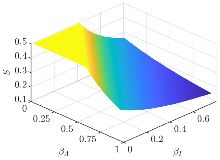
(a)

(b)

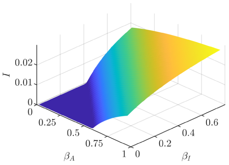
(c)

(d)

Figure 2: Asymptotic values of $S$, $A$, $I$, and $R$ as a function of $\beta_{A}$ and $\beta_{I}$. Values of the parameters: $\mu=1/(70\cdot 365)$, meaning an average lifespan of 70 years; $\beta_{A}\in[0.01,0.8]$ $\beta_{I}\in[0.01,0.95]$, $\nu=0.01$, $\gamma=1/100$, meaning the immunity lasts on average 100 days; $\alpha=0.15$, $\delta_{A}=0.1$, $\delta_{I}=0.15$.

Figures 3(a), 3(b), 3(c) and 3(d) confirm our analytical results on the asymptotic values of the fraction of individuals in each compartment. In particular, the endemic equilibrium value of $S$ (13) does not depend on $\gamma$, the loss of immunity rate, as shown by the time series corresponding to $\gamma=0.01$, $0.02$ and $0.05$, whereas the disease free equilibrium value of $S$ (4), corresponding to the $\gamma=0.001$ plot, does. Increasing the value of $\gamma$, which corresponds to decreasing the average duration $1/\gamma$ of the immunity time-window, results in bigger asymptotic values for the asymptomatic and symptomatic infected population $A$ and $I$ and in a smaller asymptotic value for the recovered population $R$. This trend is quite intuitive: indeed, by keeping the others parameters fixed, if the average immune period decreases (i.e., $\gamma$ increases), a removed individual quickly return to the susceptible state, hence the behavior of the SAIRS model approaches that of a SAIS model.

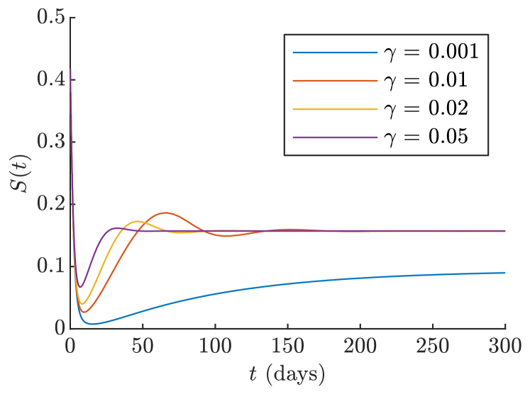
(a)

(b)

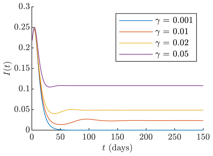
(c)

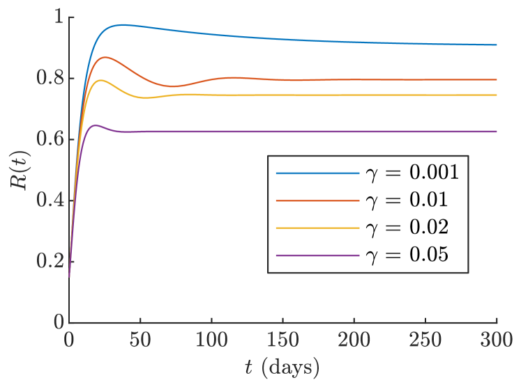
(d)

Figure 3: Behavior of system (1) as $\gamma$, the rate of loss of immunity, varies. Values of the parameters: $\mu=1/(70\cdot 365)$, meaning an average lifespan of 70 years; $\beta_{A}=0.8$ $\beta_{I}=0.95$, $\nu=0.01$, $\gamma$ varying as shown; $\alpha=0.15$, $\delta_{A}=0.125$, $\delta_{I}=0.15$.

Next, we explore the effect of changing $\alpha$, the rate of symptoms onset, in three scenarios: equally infectious asymptomatic and symptomatic individuals ($\beta_{A}=\beta_{I}$), in Figure 4; asymptomatic individuals more infectious than symptomatic individuals ($\beta_{A}>\beta_{I}$) (this case can be of interest if we consider that asymptomatic individuals can, in principle, move and spread the infection more than symptomatic ones) in Figure 5; and vice-versa ($\beta_{A}<\beta_{I}$), in Figure 6. If $\mathcal{R}_{0}>1$, $A^{*}$ and $I^{*}$ are related by $A^{*}=\frac{\delta_{I}+\mu}{\alpha}I^{*}$ (12). This means that, regardless of the values of $\beta_{A}$ and $\beta_{I}$, $A^{*}>I^{*}$ if and only if $\frac{\delta_{I}+\mu}{\alpha}>1$. This is evident in Figures 4(b), 5(b) and 6(b), where the smallest value of that ratio, corresponding to $\alpha=0.9$, is smaller than $1$, results in $I^{*}>A^{*}$; the biggest value of that ratio, and the only one significantly bigger than $1$ is attained for $\alpha=0.01$, and results in $I^{*}<A^{*}$. Increasing $\alpha$ leads to a smaller asymptotic value for $A$, and a bigger asymptotic value for $I$. Effectively, by keeping fixed the other parameters and increasing $\alpha$ leads to a decreasing of the average time-period before developing symptoms, thus the behavior of the SAIRS model approaches that of the SIRS one, as $\alpha$ increases.

Finally, in Figure 7, we compare the effect of varying $\nu$, the vaccination rate, on the epidemic dynamics. In particular, the parameter values chosen satisfy the assumption of Theorem 14, i.e. $\mathcal{R}_{0}>1$ and simultaneously $\beta_{A}<\delta_{I}$. We observe that the asymptotic values of $A$ and $I$ are decreasing in $\nu$, whereas the endemic equilibrium value of $S$ is independent from this parameter, as we expect from (13), and the endemic equilibrium value of $R$ is increasing in $\nu$.

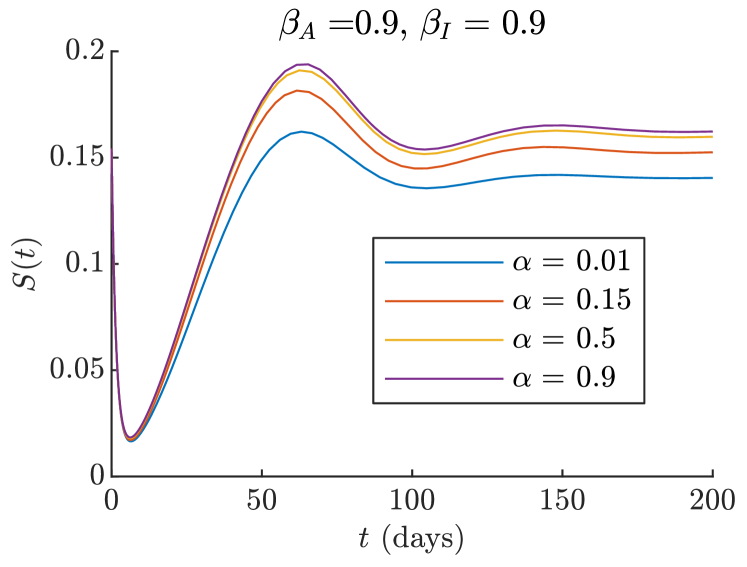
(a)

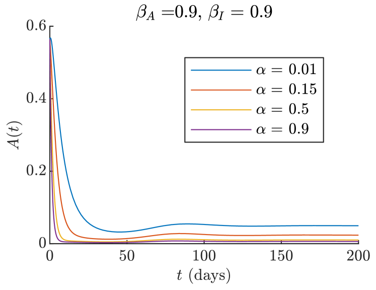
(b)

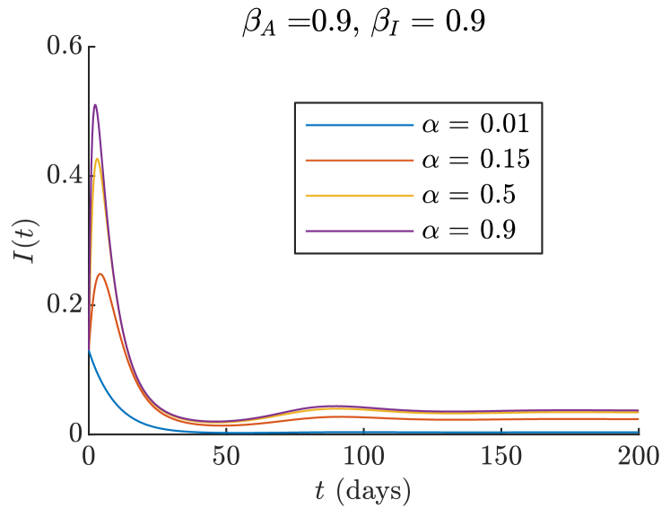
(c)

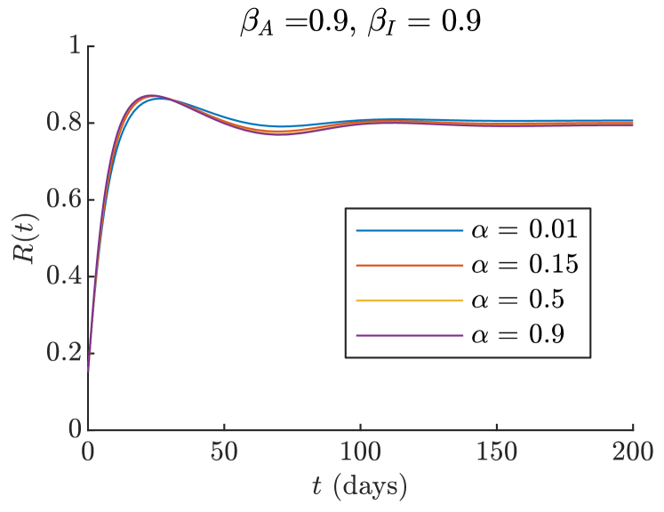
(d)

Figure 4: Behavior of system (1) as $\alpha$, the rate of symptoms onset, varies. Values of the parameters: $\mu=1/(70\cdot 365)$, meaning an average lifespan of 70 years; $\beta_{A}=\beta_{I}=0.9$, $\nu=0.01$, $\gamma=1/100$, meaning the immunity lasts on average 100 days; $\alpha$ varying as shown, $\delta_{A}=0.125$, $\delta_{I}=0.15$.

(a)

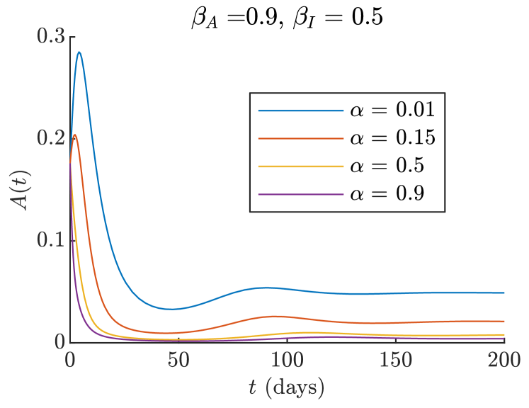
(b)

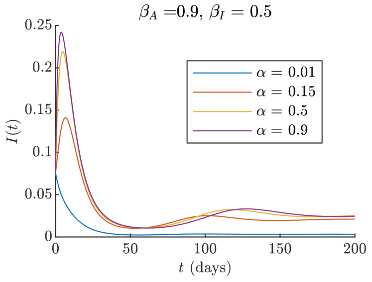
(c)

(d)

Figure 5: Behavior of system (1) as $\alpha$, the rate of symptoms onset, varies. Values of the parameters: $\mu=1/(70\cdot 365)$, meaning an average lifespan of 70 years; $\beta_{A}=0.9$ $\beta_{I}=0.5$, $\nu=0.01$, $\gamma=1/100$, meaning the immunity lasts on average 100 days; $\alpha$ varying as shown, $\delta_{A}=0.125$, $\delta_{I}=0.15$.

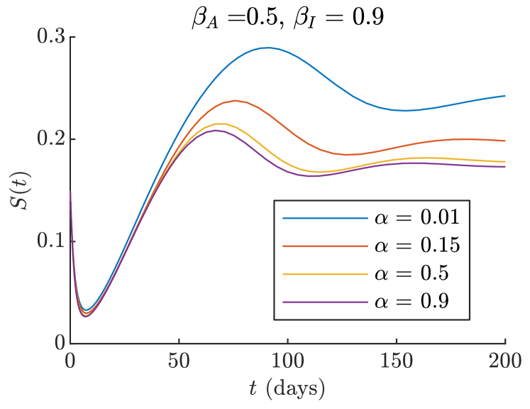
(a)

(b)

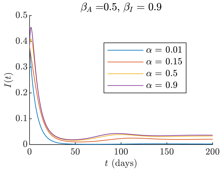
(c)

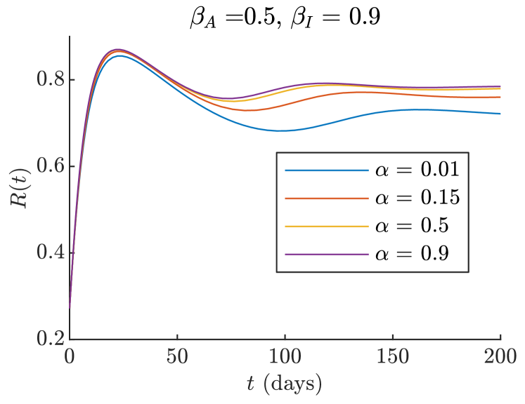
(d)

Figure 6: Behavior of system (1) as $\alpha$, the rate of symptoms onset, varies. Values of the parameters: $\mu=1/(70\cdot 365)$, meaning an average lifespan of 70 years; $\beta_{A}=0.5$ $\beta_{I}=0.9$, $\nu=0.01$, $\gamma=1/100$, meaning the immunity lasts on average 100 days; $\alpha$ varying as shown, $\delta_{A}=0.125$, $\delta_{I}=0.15$.

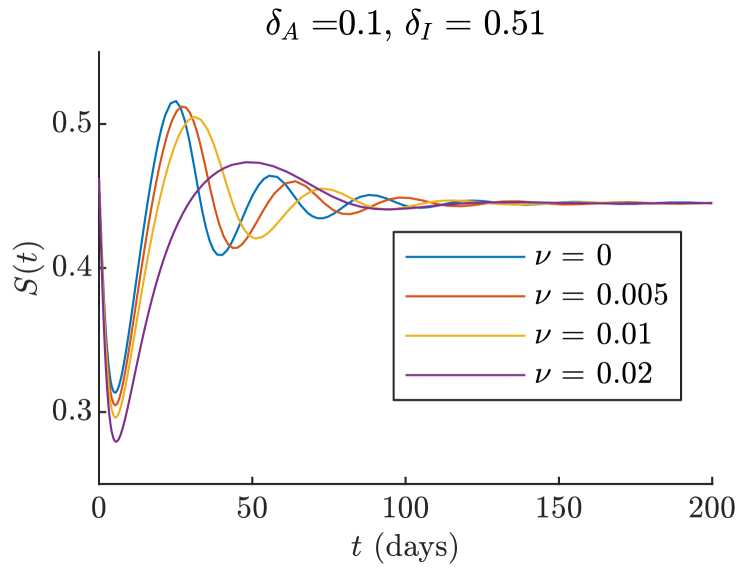
(a)

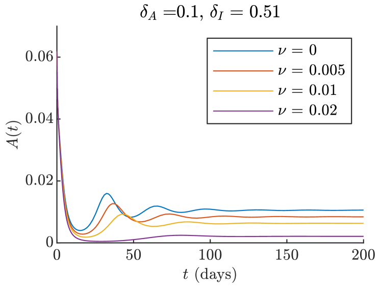
(b)

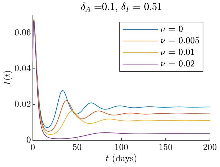
(c)

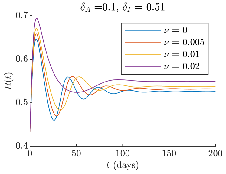
(d)

Figure 7: Behavior of system (1) as $\nu$, the vaccination rate, varies. Values of the parameters: $\mu=1/(70\cdot 365)$, meaning an average lifespan of 70 years; $\beta_{A}=0.5$ $\beta_{I}=0.9$, $\nu$ varying as shown, $\gamma=1/50$, meaning the immunity lasts on average 50 days; $\alpha=0.9$, $\delta_{A}=0.1$, $\delta_{I}=0.51$. The condition $\beta_{A}<\delta_{I}$ is satisfied.

6 Conclusions

We analyzed the behavior of an SAIRS compartmental model with vaccination. We determined the value of the basic reproduction number $\mathcal{R}_{0}$; then, we proved that the disease-free equilibrium is globally asymptotically stable, i.e.. the disease eventually dies out, if $\mathcal{R}_{0}<1$. Moreover, in the SAIRS-type model without vaccination ($\nu=0$), we were able to generalize the result on the global asymptotic stability of the DFE also in the case $\mathcal{R}_{0}=1$.

Furthermore, we proved the uniform persistence of the disease and the existence of a unique endemic equilibrium if $\mathcal{R}_{0}>1$. Later, we analyzed the stability of this endemic equilibrium for some subcases of the model.

The first case describes a disease which confers permanent immunity, i.e. $\gamma=0$: the model reduces to an SAIR. In this framework, we answered the open problem presented in [1], including the additional complexity of vaccination: we proved the global asymptotic stability of the endemic equilibrium when $\mathcal{R}_{0}>1$.

We then proceeded to extend the results provided in [11] on the local stability analysis for a SAIRS-type model. We first considered the SAIRS model with the assumption that both asymptomatic and symptomatic infectious have the same transmission rate and recovery rate, i.e. $\beta_{A}=\beta_{I}$ and $\delta_{A}=\delta_{I}$, respectively. We were able to show that the endemic equilibrium is globally asymptotically stable if $\mathcal{R}_{0}>1$. Moreover, we analyzed the model without restrictions; we used the geometric approach proposed in [30] to find the conditions under which the endemic equilibrium is globally asymptotically stable. We proved the global stability in the case $\mathcal{R}_{0}>1$ and $\beta_{A}<\delta_{I}$.

We leave, as an open problem, the global asymptotic stability of the endemic equilibrium without any restriction on the parameters: we conjecture that the global asymptotic stability for the endemic equilibrium only requires $\mathcal{R}_{0}>1$, as our numerical simulations suggest.

Many generalizations and investigations of our model are possible. For example, we considered the vital dynamics without distinguish between natural death and disease related deaths; an interesting, although complex, generalization of our model could explore the implications of including disease-induced mortality.

A natural extension of our SAIRS model could take into account different groups of individual among which an epidemic can spread. One modelling approach for this are multi-group compartmental models. Other more realistic extensions may involve a greater number of compartments, for example the “Exposed” group, or time-dependent parameters which can describe the seasonality of a disease or some response measures from the population, as well as non-pharmaceutical interventions.

References

• [1] S. Ansumali, S. Kaushal, A. Kumar, M. K. Prakash, and M. Vidyasagar, “Modelling a pandemic with asymptomatic patients, impact of lockdown and herd immunity, with applications to SARS-CoV-2,” Annual reviews in control, 2020.
• [2] A. Aleta and Y. Moreno, “Evaluation of the potential incidence of COVID-19 and effectiveness of containment measures in Spain: a data-driven approach,” BMC medicine, vol. 18, pp. 1–12, 2020.
• [3] M. Gatto, E. Bertuzzo, L. Mari, S. Miccoli, L. Carraro, R. Casagrandi, and A. Rinaldo, “Spread and dynamics of the COVID-19 epidemic in Italy: Effects of emergency containment measures,” Proceedings of the National Academy of Sciences, vol. 117, no. 19, pp. 10484–10491, 2020.
• [4] J. A. Backer and J. Wallinga, “Spatiotemporal analysis of the 2014 Ebola epidemic in West Africa,” PLoS computational biology, vol. 12, no. 12, p. e1005210, 2016.
• [5] M. Ferrari, R. Grais, N. Bharti, A. Conlan, O. N. Bjørnstad, L. J. Wolfson, P. J. Guerin, A. Djibo, and B. T. Grenfell, “The dynamics of measles in sub-Saharan Africa,” Nature, vol. 451, no. 7179, pp. 679–684, 2008.
• [6] M. Tizzoni, P. Bajardi, C. Poletto, J. J. Ramasco, D. Balcan, B. Gonçalves, N. Perra, V. Colizza, and A. Vespignani, “Real-time numerical forecast of global epidemic spreading: case study of 2009 A/H1N1pdm,” BMC medicine, vol. 10, no. 1, pp. 1–31, 2012.
• [7] M. Day, “Covid-19: identifying and isolating asymptomatic people helped eliminate virus in Italian village,” BMJ: British Medical Journal (Online), vol. 368, 2020.
• [8] K. Mizumoto, K. Kagaya, A. Zarebski, and G. Chowell, “Estimating the asymptomatic proportion of coronavirus disease 2019 (COVID-19) cases on board the Diamond Princess cruise ship, Yokohama, Japan, 2020,” Eurosurveillance, vol. 25, no. 10, p. 2000180, 2020.
• [9] D. P. Oran and E. J. Topol, “Prevalence of asymptomatic SARS-CoV-2 infection: a narrative review,” Annals of internal medicine, vol. 173, no. 5, pp. 362–367, 2020.
• [10] D. P. Oran and E. J. Topol, “The proportion of SARS-CoV-2 infections that are asymptomatic: a systematic review,” Annals of internal medicine, vol. 174, no. 5, pp. 655–662, 2021.
• [11] M. Robinson and N. I. Stilianakis, “A model for the emergence of drug resistance in the presence of asymptomatic infections,” Mathematical Biosciences, vol. 243, no. 2, pp. 163–177, 2013.
• [12] F. Débarre, S. Bonhoeffer, and R. R. Regoes, “The effect of population structure on the emergence of drug resistance during influenza pandemics,” Journal of the Royal Society Interface, vol. 4, no. 16, pp. 893–906, 2007.
• [13] J. T. Kemper, “The effects of asymptomatic attacks on the spread of infectious disease: a deterministic model,” Bulletin of mathematical biology, vol. 40, no. 6, pp. 707–718, 1978.
• [14] N. I. Stilianakis, A. S. Perelson, and F. G. Hayden, “Emergence of drug resistance during an influenza epidemic: insights from a mathematical model,” Journal of Infectious Diseases, vol. 177, no. 4, pp. 863–873, 1998.
• [15] Z. Shuai and P. van den Driessche, “Global stability of infectious disease models using Lyapunov functions,” SIAM Journal on Applied Mathematics, vol. 73, no. 4, pp. 1513–1532, 2013.
• [16] A. Korobeinikov, “Lyapunov functions and global stability for SIR and SIRS epidemiological models with non-linear transmission,” Bulletin of Mathematical Biology, vol. 68, no. 3, pp. 615–626, 2006.
• [17] J. Mena-Lorcat and H. Hethcote, “Dynamic models of infectious diseases as regulators of population sizes,” Journal of Mathematical Biology, vol. 30, no. 7, pp. 693–716, 1992.
• [18] M. Y. Li and J. S. Muldowney, “A geometric approach to global-stability problems,” SIAM Journal on Mathematical Analysis, vol. 27, no. 4, pp. 1070–1083, 1996.
• [19] M. Y. Li and J. S. Muldowney, “Dynamics of differential equations on invariant manifolds,” Journal of Differential Equations, vol. 168, no. 2, pp. 295–320, 2000.
• [20] M. Y. Li, J. R. Graef, L. Wang, and J. Karsai, “Global dynamics of a SEIR model with varying total population size,” Mathematical Biosciences, vol. 160, no. 2, pp. 191–213, 1999.
• [21] M. Li and J. Muldowney, “Global stability for the SEIR model in epidemiology,” Mathematical biosciences, vol. 125, no. 2, pp. 155–164, 1995.
• [22] P. Van den Driessche, M. Li, and J. Muldowney, “Global stability of SEIRS models in epidemiology,” Canadian Applied Mathematics Quarterly, vol. 7, pp. 409–425, 1999.
• [23] B. Buonomo and D. Lacitignola, “On the use of the geometric approach to global stability for three dimensional ODE systems: a bilinear case,” Journal of Mathematical Analysis and Applications, vol. 348, no. 1, pp. 255–266, 2008.
• [24] B. Buonomo, A. d’Onofrio, and D. Lacitignola, “Global stability of an SIR epidemic model with information dependent vaccination,” Mathematical biosciences, vol. 216, no. 1, pp. 9–16, 2008.
• [25] B. Buonomo, A. d’Onofrio, and D. Lacitignola, “Modeling of pseudo-rational exemption to vaccination for SEIR diseases,” Journal of Mathematical Analysis and Applications, vol. 404, no. 2, pp. 385–398, 2013.
• [26] G. Lu and Z. Lu, “Geometric approach for global asymptotic stability of three-dimensional Lotka–Volterra systems,” Journal of Mathematical Analysis and Applications, vol. 389, no. 1, pp. 591–596, 2012.
• [27] E. J. Nelson, J. B. Harris, J. G. Morris, S. B. Calderwood, and A. Camilli, “Cholera transmission: the host, pathogen and bacteriophage dynamic,” Nature Reviews Microbiology, vol. 7, no. 10, pp. 693–702, 2009.
• [28] V. Wiwanitkit, “Unusual mode of transmission of dengue,” The Journal of Infection in Developing Countries, vol. 4, no. 01, pp. 051–054, 2010.
• [29] Y. Gu, N. Komiya, H. Kamiya, Y. Yasui, K. Taniguchi, and N. Okabe, “Pandemic (H1N1) 2009 transmission during presymptomatic phase, Japan,” Emerging infectious diseases, vol. 17, no. 9, p. 1737, 2011.
• [30] G. Lu and Z. Lu, “Geometric approach to global asymptotic stability for the SEIRS models in epidemiology,” Nonlinear Analysis: Real World Applications, vol. 36, pp. 20–43, 2017.
• [31] J. A. Yorke, “Invariance for ordinary differential equations,” Theory of Computing Systems, vol. 1, no. 4, pp. 353–372, 1967.
• [32] R. M. Anderson and R. M. May, Infectious diseases of humans: dynamics and control. Oxford university press, 1992.
• [33] O. Diekmann and J. A. P. Heesterbeek, Mathematical epidemiology of infectious diseases: model building, analysis and interpretation, vol. 5. John Wiley & Sons, 2000.
• [34] P. van den Driessche and J. Watmough, “Further notes on the basic reproduction number,” in Mathematical Epidemiology, pp. 159–178, Springer, 2008.
• [35] P. van den Driessche and J. Watmough, “Reproduction numbers and sub-threshold endemic equilibria for compartmental models of disease transmission,” Mathematical Biosciences, vol. 180, pp. 29–48, 2002.
• [36] L. Perko, “Linear systems,” in Differential Equations and Dynamical Systems, pp. 1–63, Springer, 1991.
• [37] H. I. Freedman, S. Ruan, and M. Tang, “Uniform persistence and flows near a closed positively invariant set,” Journal of Dynamics and Differential Equations, vol. 6, no. 4, pp. 583–600, 1994.
• [38] N. P. Bhatia and G. P. Szegö, Dynamical systems: stability theory and applications, vol. 35. Springer, 2006.
• [39] J. P. La Salle, The stability of dynamical systems. SIAM, 1976.
• [40] M. Ballyk, C. C. McCluskey, and G. S. Wolkowicz, “Global analysis of competition for perfectly substitutable resources with linear response,” Journal of mathematical biology, vol. 51, no. 4, pp. 458–490, 2005.
• [41] H. Guo, M. Y. Li, and Z. Shuai, “Global stability of the endemic equilibrium of multigroup SIR epidemic models,” Canadian applied mathematics quarterly, vol. 14, no. 3, pp. 259–284, 2006.