Measuring Sample Quality in Algorithms for Intractable Normalizing Function Problems

Abstract

Models with intractable normalizing functions have numerous applications. Because the normalizing constants are functions of the parameters of interest, standard Markov chain Monte Carlo cannot be used for Bayesian inference for these models. A number of algorithms have been developed for such models. Some have the posterior distribution as their asymptotic distribution. Other “asymptotically inexact” algorithms do not possess this property. There is limited guidance for evaluating approximations based on these algorithms. Hence it is very hard to tune them. We propose two new diagnostics that address these problems for intractable normalizing function models. Our first diagnostic, inspired by the second Bartlett identity, is in principle broadly applicable to Monte Carlo approximations beyond the normalizing function problem. We develop an approximate version of this diagnostic that is applicable to intractable normalizing function problems. Our second diagnostic is a Monte Carlo approximation to a kernel Stein discrepancy-based diagnostic introduced by Gorham and Mackey (2017). We provide theoretical justification for our methods and apply them to several algorithms in challenging simulated and real data examples including an Ising model, an exponential random graph model, and a Conway–Maxwell–Poisson regression model, obtaining interesting insights about the algorithms in these contexts.

Keywords: Bartlett identity, Doubly intractable distributions, Kernel Stein discrepancy, Markov chain Monte Carlo, Sample quality measure

1 Introduction

Models with intractable normalizing functions arise in many contexts, notably the Ising (Lenz,, 1920; Ising,, 1925) and autologistic models (see Besag,, 1974; Hughes et al.,, 2011, for a review) for binary data on a lattice, exponential random graph models (see Robins et al.,, 2007; Hunter and Handcock,, 2006) and mixed graphical models (see Lauritzen and Wermuth,, 1989; Lee and Hastie,, 2015; Cheng et al.,, 2017) for explaining relationships among actors in networks, interaction point process models (see Strauss,, 1975; Goldstein et al.,, 2015) for describing spatial patterns among points, and Conway–Maxwell-Poisson regression models (see Conway and Maxwell,, 1962; Shmueli et al.,, 2005; Chanialidis et al.,, 2018) for over- or under-dispersed count data. Interest in models having intractable normalizing functions has increased rapidly during the last two decades. Indeed, a look at the Web of Science database shows that the number of yearly citations of articles on this subject has grown quadratically since 2005. Unfortunately, standard Markov chain Monte Carlo (MCMC) algorithms, the workhorse of Bayesian inference in the past few decades, cannot be applied to these models. Suppose we have data $\boldsymbol{x}\in\mathcal{X}$ generated from a probability model $f(\boldsymbol{x}\mid\boldsymbol{\theta})$ with likelihood function $L(\boldsymbol{\theta}\mid\boldsymbol{x})=h(\boldsymbol{x}\mid\boldsymbol{\theta})/c(\boldsymbol{\theta})$, where $c(\boldsymbol{\theta})$ is a normalizing function, and a prior density $p(\boldsymbol{\theta})$. The posterior density of $\boldsymbol{\theta}$ is $\pi(\boldsymbol{\theta}\mid\boldsymbol{x})\propto p(\boldsymbol{\theta})h(\boldsymbol{x}\mid\boldsymbol{\theta})/c(\boldsymbol{\theta})$, which brings about so-called doubly intractable posterior distributions. A major problem in constructing a standard MCMC algorithm for such models is that $c(\boldsymbol{\theta})$ cannot be easily evaluated. The Metropolis–Hastings (MH) algorithm (Metropolis et al.,, 1953; Hastings,, 1970) acceptance probability at each step requires evaluating the unknown ratio $c(\boldsymbol{\theta})/c(\boldsymbol{\theta}^{\prime})$, where $\boldsymbol{\theta}^{\prime}$ denotes the proposed value.

A wide range of computational methods have been proposed for Bayesian inference for doubly intractable posterior distributions (see Park and Haran,, 2018, for a review). There are asymptotically exact algorithms whose Markov chain has a stationary distribution equal to its target distribution (cf. Møller et al.,, 2006; Murray et al.,, 2006; Atchadé et al.,, 2013; Lyne et al.,, 2015; Liang et al.,, 2016). Throughout this manuscript we use “target distribution” to refer to the posterior distribution of interest. Some of the asymptotically exact algorithms are available only for a small class of probability models having intractable normalizing functions. The other algorithms are complicated to construct and have to be carefully tuned to provide reliable inference. These algorithms tend to be computationally intensive (Park and Haran,, 2018). There are asymptotically inexact algorithms that may be much faster and can be applied to a wider class of problems (cf. Liang,, 2010; Alquier et al.,, 2016; Park and Haran,, 2020). An asymptotically inexact algorithm either converges to an approximation of the target or is not known to converge to any distribution. The performance of these algorithms relies on the choice of various tuning parameters. It is also not always easy to judge the tradeoffs between using a faster asymptotically inexact algorithm and a potentially more computationally expensive but asymptotically exact algorithm. Hence, it is crucial to have diagnostics that provide guidance for users to carefully tune their algorithms to provide reliable results.

There is a large literature on convergence diagnostics for MCMC algorithms (see Cowles and Carlin,, 1996; Flegal and Jones,, 2011; Roy,, 2020, for a review). In fact, given the wide usage of MCMC and the importance of MCMC diagnostics, some of the best known MCMC diagnostics papers have thousands of citations (cf. Gelman and Rubin,, 1992; Geyer,, 1992; Geweke et al.,, 1991) and at this point perhaps often even get used without citation. However, the literature on assessing the quality of approximations provided by asymptotically inexact algorithms is very limited. There are several approaches that measure the deviation between sample means and target expectations whose values are known (Fan et al.,, 2006; Gorham and Mackey,, 2015, 2017). Lee et al., (2019) and Xing et al., (2019) have provided tools for assessing the coverage of approximate credible intervals. These are laudable innovations, but they are not available for asymptotically inexact algorithms for doubly intractable distributions. This motivates our development of sample quality measures that assist scientists in tuning these algorithms.

In this article we describe a new diagnostic method that uses the well known second Bartlett identity (Bartlett, 1953a, ; Bartlett, 1953b, ). Our method is, in principle, applicable in virtually any likelihood-based context where misspecification is of concern. We develop a Monte Carlo approximation to this new diagnostic that is applicable to intractable normalizing function models. We also develop an approximate version of the kernel Stein discrepancy introduced by Gorham and Mackey, (2017), making this available for doubly intractable distributions. This diagnostic asymptotically inherits the same convergence properties as that of Gorham and Mackey, (2017) and thus can be used for diagnosing convergence of a sequence of sample distributions to the target distribution. Following Gorham and Mackey, (2017), we think of our diagnostics as measuring “sample quality.”

The remainder of this article is organized as follows. In Section 2 we briefly describe computational methods for models with intractable normalizing functions. In Section 3 we discuss the need for diagnostics for tuning asymptotically inexact algorithms. In Section 4 we propose a new diagnostic for asymptotically exact and inexact methods, and we develop an approximation for doubly intractable distributions. In Section 5 we briefly describe the kernel Stein discrepancy introduced by Gorham and Mackey, (2017) and propose its Monte Carlo approximation for intractable normalizing function models. We provide theoretical justification for our diagnostics. In Section 6 we describe the application of our diagnostic approaches to several algorithms in the context of three different challenging examples and study the computational complexity and variability of our diagnostics. Finally, in Section 7 we conclude with a brief summary and discussion.

2 Inference for Models with Intractable Normalizing Functions

Several computational methods have been developed for Bayesian inference for models with intractable normalizing functions. Park and Haran, (2018) categorized these algorithms into two general, overlapping classes: (1) auxiliary variable approaches, which introduce an auxiliary variable and cancel out the normalizing functions in the Metropolis–Hastings acceptance probability (Møller et al.,, 2006; Murray et al.,, 2006; Liang,, 2010; Liang et al.,, 2016), and (2) likelihood approximation approaches, which directly approximate the normalizing functions and plug the approximations into the Metropolis–Hastings acceptance probability (Atchadé et al.,, 2013; Lyne et al.,, 2015; Alquier et al.,, 2016; Park and Haran,, 2020). An important characteristic of these algorithms is whether they are “asymptotically exact” or “asymptotically inexact.” Asymptotically exact algorithms generate a sequence whose asymptotic distribution is exactly equal to the target distribution. Asymptotically inexact algorithms generate a sequence that does not converge to the target distribution (or to any distribution in some cases).

Asymptotically exact algorithms have attractive theoretical properties but can often be computationally burdensome or even infeasible for challenging models. For instance, Møller et al., (2006) and Murray et al., (2006) depend on perfect sampling (cf. Propp and Wilson,, 1996), an algorithm that generates an auxiliary variable exactly from the target distribution using bounding Markov chains. Perfect samplers tend to be very computationally expensive and are available only for a small class of probability models. Atchadé et al., (2013) and Liang et al., (2016) propose asymptotically exact algorithms that do not need perfect sampling. Atchadé et al., (2013)’s adaptive MCMC (ALR) algorithm introduces multiple particles $\boldsymbol{\theta}^{(1)},\dots,\boldsymbol{\theta}^{(d)}$ over the parameter space and approximates $c(\boldsymbol{\theta})$ in the acceptance probability through importance sampling using the entire sample path of the algorithm. Liang et al., (2016)’s adaptive exchange (AEX) algorithm runs an auxiliary chain and a target chain simultaneously. At each iteration, the auxiliary chain simulates and stores a sample from a set of distributions, $\{h(\boldsymbol{x}\mid\boldsymbol{\theta}^{(1)})/c(\boldsymbol{\theta}^{(1)})$, $\dots$, $h(\boldsymbol{x}\mid\boldsymbol{\theta}^{(d)})/c(\boldsymbol{\theta}^{(d)})\}$, where $\boldsymbol{\theta}^{(1)}$, $\dots$, $\boldsymbol{\theta}^{(d)}$ are predetermined particles over the parameter space. The target chain generates a posterior sample via the exchange algorithm (Murray et al.,, 2006), where an auxiliary variable $\boldsymbol{y}$ is sampled from the cumulative samples in the auxiliary chain instead of exact sampling of $\boldsymbol{y}$. These algorithms require storing simulated auxiliary data or their sufficient statistics with each iteration. The computational and memory costs are very expensive for models without low-dimensional sufficient statistics. Pseudo-marginal MCMC algorithms (Beaumont,, 2003; Andrieu and Roberts,, 2009) are approaches that use an unbiased Monte Carlo approximation of an intractable likelihood. Lyne et al., (2015) constructed an unbiased likelihood estimate for models with intractable normalizing functions. To obtain a single estimate, their approach requires multiple Monte Carlo approximations to the normalizing constant and thus can often be computationally prohibitive.

Several computationally efficient asymptotically inexact algorithms have also been proposed. For instance, the double Metropolis–Hastings (DMH) sampler, proposed by Liang, (2010), replaces perfect sampling with a standard Metropolis–Hastings algorithm, an “inner sampler,” at each iteration of the exchange algorithm. The DMH algorithm is easy to implement and is computationally efficient compared to the other algorithms discussed thus far. But the inner sampling becomes more computationally expensive with an increase in the dimension of the data. For large data problems, Park and Haran, (2020) proposed a function emulation algorithm that approximates the likelihood normalizing function (or full likelihood function) at several parameter values and interpolates the function using a Gaussian process. This provides significant gains in computational efficiency. More asymptotically exact and inexact algorithms are found in Park and Haran, (2018).

Both asymptotically exact and inexact algorithms require careful tuning in order to provide good approximations in a reasonable amount of time. For instance, the ALR and AEX algorithms require users to select an appropriate number $d$ of particles to cover the important region of the parameter space. The DMH algorithm requires users to decide the length $m$ of the inner sampler for generating an auxiliary variable. As $m$ grows large the auxiliary variable becomes approximately a draw from the probability model at the expense of longer computing time. However, currently there is little guidance on how to tune these algorithms, and most of them rely on simulation studies. Also, the behavior of the algorithm varies across models or across datasets for a given model.

3 The Need for Diagnostics for Intractable Normalizing Function Problems

There is a vast literature on MCMC convergence diagnostics (see Cowles and Carlin,, 1996; Flegal and Jones,, 2011; Roy,, 2020, for a review). However, these diagnostics may not be adequate for asymptotically inexact algorithms. Suppose we have a sample generated by an asymptotically inexact method. Such a sample may not have an asymptotic distribution, or said sample may converge but to a mere approximation of the target distribution. Standard MCMC diagnostics assess whether the sample has converged to its asymptotic distribution but do not assess whether the asymptotic distribution is equal to the target distribution. As discussed in Section 2, however, asymptotically exact algorithms for models with intractable normalizing functions are available only for a few special cases, and even for these cases computing tends to be quite burdensome.

Several approaches based on measuring the difference between sample means and target expectations have been proposed for assessing the quality of approximations provided by asymptotically inexact algorithms. Fan et al., (2006) proposed score function diagnostics for assessing estimates of some quantities the values of which are known under the target distribution. They suggested plotting the Monte Carlo estimate versus the sample size together with error bounds. Gorham and Mackey, (2015) pointed out limitations of the score function diagnostics caused by considering only a finite class of functions and introduced a new diagnostic method based on a Stein discrepancy. Gorham and Mackey, (2015) defined Stein discrepancies that bound the discrepancy between the sample mean and the target expectation over a large collection of functions whose target expectations are zero. The Stein discrepancies are supported by a theory of weak convergence and are attainable by solving a linear program. Combining this idea with the theory of reproducing kernels, Gorham and Mackey, (2017) provided a closed-form kernel Stein discrepancy with sound theoretical support analogous to that of Gorham and Mackey, (2015) (see Section 5.1 for details). These approaches are useful for comparing asymptotically approximate samplers and for selecting tuning parameters for such samplers. However, all of them require evaluating the score function of the target density, which is not possible for doubly intractable posterior distributions. In contrast, our approaches apply broadly to asymptotically exact and inexact algorithms even for such challenging problems. To our knowledge, no other diagnostics are currently available for asymptotically inexact algorithms for intractable normalizing function models. We have studied our diagnostics as applied in several challenging real data settings. In addition, we provide theoretical justification for our methods.

4 Curvature Diagnostics

In this section we introduce two new diagnostics that are useful for tuning asymptotically exact and inexact algorithms: a curvature diagnostic (CD) and an approximate curvature diagnostic (ACD). The curvature diagnostic is based on the second Bartlett identity from the classical theory of maximum likelihood. The approximate curvature diagnostic is an approximation of the CD that is suitable for intractable normalizing function problems.

4.1 A General Purpose Curvature Diagnostic

Consider a sequence of sample points $\boldsymbol{\theta}^{(1)},\dots,\boldsymbol{\theta}^{(n)}$ generated by an algorithm having $\pi(\boldsymbol{\theta}\mid\boldsymbol{x})$ as its target distribution. Our aim is to determine whether the sample will produce a good approximation to some quantity of interest, e.g., $\textup{E}_{\pi}\{z(\boldsymbol{\theta})\}$, where $z(\boldsymbol{\theta})$ is a real-valued function. Our diagnostic, the curvature diagnostic, is inspired by the method for obtaining the asymptotic variance of a maximum likelihood estimator under a misspecified model. When the model is misspecified, the second Bartlett identity does not hold, which is to say (see details below) the sensitivity matrix is not equal to the variability matrix. And so the asymptotic variance of the estimator does not simplify to the inverse of the Fisher information. Our curvature diagnostic uses the dissimilarity between the sensitivity matrix and the variability matrix to assess the quality of the sample. We provide details in the following paragraph.

Let $\boldsymbol{u}(\boldsymbol{\theta})=\nabla_{\boldsymbol{\theta}}\log\pi(\boldsymbol{\theta}\mid\boldsymbol{x})$ be the score function of the posterior density $\pi(\boldsymbol{\theta}\mid\boldsymbol{x})$. The posterior density has the sensitivity matrix

$$\textup{E}_{\pi}\left\{-\frac{\partial}{\partial\boldsymbol{\theta}}\boldsymbol{u}(\boldsymbol{\theta})\right\} =\int_{\boldsymbol{\Theta}}-\frac{\partial}{\partial\boldsymbol{\theta}}\boldsymbol{u}(\boldsymbol{\theta})\pi(\boldsymbol{\theta}\mid\boldsymbol{x})d\boldsymbol{\theta}$$

and the variability matrix $\textup{var}_{\pi}\left\{\boldsymbol{u}(\boldsymbol{\theta})\right\}=\textup{E}_{\pi}\left\{\boldsymbol{u}(\boldsymbol{\theta})\boldsymbol{u}(\boldsymbol{\theta})^{\top}\right\}$. Note that the identity for the variability matrix follows from Bartlett’s first identity: $\textup{E}_{\pi}\{\boldsymbol{u}(\boldsymbol{\theta})\}=\textbf{0}$. Let $H(\boldsymbol{\theta})=\frac{\partial}{\partial\boldsymbol{\theta}}\boldsymbol{u}(\boldsymbol{\theta})$, $J(\boldsymbol{\theta})=\boldsymbol{u}(\boldsymbol{\theta})\boldsymbol{u}(\boldsymbol{\theta})^{\top}$, and $\boldsymbol{d}(\boldsymbol{\theta})=\textup{vech}[J(\boldsymbol{\theta})+H(\boldsymbol{\theta})]$, where $\textup{vech}(M)$ denotes the half-vectorization of the matrix $M$. We have $\textup{E}_{\pi}\{\boldsymbol{d}(\boldsymbol{\theta})\}=\textbf{0}$ by Bartlett’s second identity: $\textup{E}_{\pi}\{-H(\boldsymbol{\theta})\}=\textup{E}_{\pi}\{J(\boldsymbol{\theta})\}$. Using the sample $\boldsymbol{\theta}^{(1)},\dots,\boldsymbol{\theta}^{(n)}$ we construct a Monte Carlo approximation to the half-vectorized difference between the sensitivity and variability matrices as

$$\boldsymbol{d}_{n} :=\frac{1}{n}\sum_{i=1}^{n}\boldsymbol{d}(\boldsymbol{\theta}^{(i)}).$$ (1)

Suppose the samples $\boldsymbol{\theta}^{(1)},\dots,\boldsymbol{\theta}^{(n)}$ are independent. By the central limit theorem, we have

$$\sqrt{n}\boldsymbol{d}_{n} \stackrel{{\scriptstyle d}}{{\to}}\textup{N}(\textbf{0},V),$$

where $V:=\textup{cov}_{\pi}\{\boldsymbol{d}(\boldsymbol{\theta})\}=\textup{E}_{\pi}\left\{\boldsymbol{d}(\boldsymbol{\theta})\boldsymbol{d}(\boldsymbol{\theta})^{\top}\right\}$. Our unbiased and consistent approximation of $V$ is calculated as

$$V_{n} :=\frac{1}{n}\sum_{i=1}^{n}\boldsymbol{d}(\boldsymbol{\theta}^{(i)})\boldsymbol{d}(\boldsymbol{\theta}^{(i)})^{\top}.$$ (2)

If $\boldsymbol{\theta}^{(1)},\dots,\boldsymbol{\theta}^{(n)}$ are from a Markov process and thus dependent, then by the Markov chain Monte Carlo central limit theorem we have

$$\sqrt{n}\boldsymbol{d}_{n}\stackrel{{\scriptstyle d}}{{\to}}\textup{N}(\textbf{0},\Sigma),$$

where $\Sigma:=\textup{cov}_{\pi}\{\boldsymbol{d}(\boldsymbol{\theta}^{(i)})\}+2\sum_{k=1}^{\infty}\textup{cov}_{\pi}\{\boldsymbol{\theta}^{(i)},\boldsymbol{\theta}^{(i+k)}\}$. The asymptotic covariance matrix $\Sigma$ can be estimated by the multivariate batch means method (Chen and Seila,, 1987; Flegal and Jones,, 2011). Let $n=a_{n}b_{n}$ where $a_{n}$ is the number of batches and $b_{n}$ is the batch size. The batch means estimate of $\Sigma$ is calculated as

$$\Sigma_{n}:=\frac{b_{n}}{a_{n}-1}\sum_{j=1}^{a_{n}}(\bar{\boldsymbol{d}}^{j}_{b_{n}}-\boldsymbol{d}_{n})(\bar{\boldsymbol{d}}^{j}_{b_{n}}-\boldsymbol{d}_{n})^{\top},$$ (3)

where $\bar{\boldsymbol{d}}^{j}_{b_{n}}=\sum_{i=(j-1)b_{n}+1}^{jb_{n}}\boldsymbol{d}(\boldsymbol{\theta}^{(i)})$. The batch means estimator is strongly consistent under some conditions (Damerdji,, 1994; Jones et al.,, 2006; Vats et al.,, 2019). Because it is simple to construct and appears to work well in practice under quite a wide range of settings (cf. Flegal et al.,, 2008), we suggest using batch means. Our curvature diagnostic is then defined as follows.

Definition 1 (Curvature Diagnostic (CD)).

Consider a sample $\boldsymbol{\theta}^{(1)}$, $\dots$, $\boldsymbol{\theta}^{(n)}$ generated by an algorithm having $\pi(\boldsymbol{\theta}\mid\boldsymbol{x})$ as its target. If the sample is independent, our curvature diagnostic is defined as $\mathcal{C}_{n}(\boldsymbol{x}):=n\boldsymbol{d}_{n}^{\top}V_{n}^{-1}\boldsymbol{d}_{n}$. If the sample is from a Markov process, our curvature diagnostic is defined as $\mathcal{C}^{\textup{BM}}_{n}(\boldsymbol{x}):=n\boldsymbol{d}_{n}^{\top}\Sigma_{n}^{-1}\boldsymbol{d}_{n}$.

The CD has an asymptotic $\chi^{2}(r)$ distribution, where $r=p(p+1)/2$ and $p$ is the dimension of $\boldsymbol{\theta}$, if the asymptotic distribution of the sample is equal to the target distribution. A simple and effective heuristic for determining $n$ is to plot $\hat{V}_{n}$ against the posterior sample size $n$ and select $n$ at which the approximations appear to have stabilized. Given $n$, an abnormally large value of CD with respect to $\chi^{2}(r)$ can signal poor sample quality. We use the $1-\alpha$ quantile of the $\chi^{2}(r)$ as a threshold for our diagnostic. A sample path for which the CD value is below the threshold is considered to have an asymptotic distribution that is reasonably close to the target distribution. We found that $\alpha=0.01$ performed well in our simulation experiments, and so we take $\alpha$ = 0.01 in the sequel.

We note that our curvature diagnostic is, in principle, applicable not only in intractable normalizing function problems but in virtually any likelihood-based context where misspecification is of concern. Moreover, the framework we present in this article can be extended to incorporate higher moments.

4.2 An Approximate Curvature Diagnostic for Intractable Normalizing Function Problems

If the normalizing function $c(\boldsymbol{\theta})$ of the likelihood is intractable, it is not possible to evaluate the curvature diagnostic since the diagnostic involves $\nabla_{\boldsymbol{\theta}}\log c(\boldsymbol{\theta})$, $\left\{\nabla_{\boldsymbol{\theta}}\log c(\boldsymbol{\theta})\right\}\left\{\nabla_{\boldsymbol{\theta}}\log c(\boldsymbol{\theta})\right\}^{\top}$, and $\partial\nabla_{\boldsymbol{\theta}}\log c(\boldsymbol{\theta})/\partial\boldsymbol{\theta}$. We therefore replace them with their Monte Carlo approximations using auxiliary variables $\boldsymbol{y}^{(1)},\dots,\boldsymbol{y}^{(N)}$ that are generated exactly from $f(\cdot\mid\boldsymbol{\theta})$ or generated by a Monte Carlo algorithm having $f(\cdot\mid\boldsymbol{\theta})$ as its target distribution. We provide details in Appendix A. By plugging these approximations into $\boldsymbol{d}(\boldsymbol{\theta})$ we obtain its approximation $\hat{\boldsymbol{d}}_{N}(\boldsymbol{\theta})$. By replacing $\boldsymbol{d}(\boldsymbol{\theta})$ with its approximation $\hat{\boldsymbol{d}}_{N}(\boldsymbol{\theta})$ in (1), (2), and (3) we obtain $\hat{\boldsymbol{d}}_{n,N}$, $\hat{V}_{n,N}$, and $\hat{\Sigma}_{n,N}$. We note that the number $a_{n,N}$ of batches and the length $b_{n,N}$ of each batch depend on $n$ and $N$ for $\hat{\Sigma}_{n,N}$. Then an approximate version of the curvature diagnostic for intractable normalizing function problems can be defined as follows.

Definition 2 (Approximate Curvature Diagnostic (ACD)).

Consider a sample $\boldsymbol{\theta}^{(1)}$, $\dots$, $\boldsymbol{\theta}^{(n)}$ generated by an algorithm having $\pi(\boldsymbol{\theta}\mid\boldsymbol{x})$ as its target. If the sample is independent, our approximate curvature diagnostic is defined as $\mathcal{\hat{C}}_{n,N}(\boldsymbol{x}):=n\>\hat{\boldsymbol{d}}_{n,N}^{\top}\hat{V}_{n,N}^{-1}\hat{\boldsymbol{d}}_{n,N}$. If the sample is from a Markov process, our approximate curvature diagnostic is defined as $\mathcal{\hat{C}}^{\textup{BM}}_{n,N}(\boldsymbol{x}):=n\>\hat{\boldsymbol{d}}_{n,N}^{\top}\hat{\Sigma}_{n,N}^{-1}\hat{\boldsymbol{d}}_{n,N}$.

To provide theoretical justification for $\mathcal{\hat{C}}_{n,N}(\boldsymbol{x})$, we make the following assumptions regarding the prior density $p(\boldsymbol{\theta})$ and the unnormalized probability model density $h(\boldsymbol{x}\mid\boldsymbol{\theta})$. We use $\|\cdot\|_{\max}$ to represent the max norm of vectors or matrices.

Assumption 1.

There exist constants $c_{p}^{\prime}$ and $c_{p}^{\prime\prime}$ such that $\|\nabla_{\boldsymbol{\theta}}\log p(\boldsymbol{\theta})\|_{\max}\leq c_{p}^{\prime}$ and $\|$ $\frac{\partial}{\partial\boldsymbol{\theta}}$ $\nabla_{\boldsymbol{\theta}}$ $\log p(\boldsymbol{\theta})$ $\|_{\max}$ $\leq c_{p}^{\prime\prime}$.

Assumption 2.

There exist constants $c_{h}^{\prime}$ and $c_{h}^{\prime\prime}$ such that $\|\nabla_{\boldsymbol{\theta}}\log h(\boldsymbol{x}\mid\boldsymbol{\theta})\|_{\max}\leq c_{h}^{\prime}$ and $\|$ $\frac{\partial}{\partial\boldsymbol{\theta}}$ $\nabla_{\boldsymbol{\theta}}$ $\log h(\boldsymbol{x}\mid\boldsymbol{\theta})$ $\|_{\max}$ $\leq c_{h}^{\prime\prime}$.

Since the prior density is determined by the user, the prior’s score function and Hessian matrix may be assumed to be bounded. In many applications Assumption 2 may be checked easily. In particular, Assumption 2 is satisfied with high probability for exponential families. For a probability model in an exponential family, the model’s score is its summary statistics and the first inequality of Assumption 2 is satisfied with high probability (Chazottes et al.,, 2007). The model’s Hessian matrix is zero and the second inequality is satisfied almost surely. Under these assumptions, Theorem 1 quantifies the distance between the asymptotic covariance matrix $V$ and its two-stage approximation $\hat{V}_{n,N}$.

Theorem 1.

Consider an i.i.d. sample $\boldsymbol{\theta}^{(1)},\dots,\boldsymbol{\theta}^{(n)}$ the asymptotic distribution of which is $\pi(\boldsymbol{\theta}\mid\boldsymbol{x})$. If Assumptions 1 and 2 hold, we have $\|\hat{V}_{n,N}-V\|_{\max}\leq\mathcal{O}\left(n^{-1/2}\right)+\mathcal{O}\left(N^{-1/2}\right)$ almost surely.

A proof of Theorem 1 is provided in Appendix B. Provided the theorem holds, the two-stage approximation $\hat{V}_{n,N}$ will get closer to $V$ as the posterior sample size $n$ and the auxiliary sample size $N$ increase.

To provide theoretical justification for $\mathcal{\hat{C}}^{\textup{BM}}_{n,N}(\boldsymbol{x})$, we make the following assumption in addition to Conditions 1 and 2 of Vats et al., (2019).

Assumption 3.

The batch size $b_{n,N}$ is an integer sequence that satisfies $b_{n,N}\to\infty$ and $(b_{n,N}/N)^{1/2}$ $\to$ $0$ as $N$ $\to$ $\infty$ and $n$ $\to$ $\infty$.

Under Assumptions 1, 2, and 3 and Conditions 1 and 2 of Vats et al., (2019), Theorem 2 quantifies the distance between $\Sigma$ and $\hat{\Sigma}_{n,N}$.

Theorem 2.

Consider a sample $\boldsymbol{\theta}^{(1)},\dots,\boldsymbol{\theta}^{(n)}$ generated from a Markov process that is an $\pi$-invariant polynomially ergodic and of order $m>(1+\epsilon_{1})(1+2/\delta)$ for some $\epsilon_{1}>0$ and $\delta>0$. Then Condition 1 of Vats et al., (2019) holds with $\gamma(n)=n^{1/2-\lambda}$ for some $\lambda>0$. If Assumptions 1, 2, and 3, and Condition 2 of Vats et al., (2019) hold, we have

$$\|\hat{\Sigma}_{n,N}-\Sigma\|_{\max} \leq\mathcal{O}\left[\{(\log n)/b_{n,N}\}^{1/2}n^{1/2-\lambda}\right]+\mathcal{O}\left[(b_{n,N}/N)^{1/2}\right]$$

almost surely.

A proof of Theorem 2 is provided in Appendix C. Provided the theorem holds, the two-stage approximation $\hat{\Sigma}_{n,N}$ will get closer to $\Sigma$ as the posterior sample size $n$ and the auxiliary sample size $N$ increase.

A simple heuristic for determining $N$ is to plot the approximation $\hat{\boldsymbol{d}}_{N}(\boldsymbol{\theta})$ against the auxiliary sample size $N$ and select $N$ at which the approximation appears to stabilize. Similarly we choose $n$ at which the approximation $\hat{V}_{n,N}$ or $\hat{\Sigma}_{n,N}$ appears to stabilize for the pre-determined $N$. We henceforth take the batch size to be $b_{n,N}=\min\{n^{1/3},N^{1/3}\}$ which satisfies Assumption 3 and Condition 2 of Vats et al., (2019).

5 A Kernel Stein Discrepancy

In this section we briefly describe an inverse multiquadric kernel Stein discrepancy (IMQ KSD) introduced by Gorham and Mackey, (2017) which is a kernel Stein discrepancy-based diagnostic for assessing the convergence of a sequence of sample distributions to its target distribution and has theoretical support. To make this approach available for doubly intractable target distributions, we develop its Monte Carlo approximation, AIKS (approximate inverse multiquadric kernel Stein discrepancy) and show that it asymptotically inherits the same convergence properties as IMQ KSD.

5.1 An Inverse Multiquadric Kernel Stein Discrepancy

Consider a target distribution $P$ with probability density function $\pi(\boldsymbol{\theta})$ under which direct integration is infeasible. Consider an i.i.d. sample $\boldsymbol{\theta}^{(1)},\dots,\boldsymbol{\theta}^{(n)}$ generated from an algorithm targeting $P$. Let $Q_{n}=\sum_{i=1}^{n}q_{n}(\boldsymbol{\theta}^{(i)})\delta_{\boldsymbol{\theta}^{(i)}}$ be a weighted sample with probability mass function $q_{n}$. Suppose we want to evaluate $\textup{E}_{P}\left\{z(\boldsymbol{\theta})\right\}$, which is intractable. The weighted sample $Q_{n}$ provides an approximation $\textup{E}_{Q_{n}}\left\{z(\boldsymbol{\theta})\right\}=\sum_{i=1}^{n}z(\boldsymbol{\theta}^{(i)})q_{n}(\boldsymbol{\theta}^{(i)})$ of the target expectation. To assess the quality of the approximation, one may consider discrepancies quantifying the maximum expectation error over a set of test functions $\mathcal{Z}$: $d_{\mathcal{Z}}(Q_{n},P)=\sup_{z\in\mathcal{Z}}\left|\textup{E}_{P}\left\{z(\boldsymbol{\theta})\right\}-\textup{E}_{Q_{n}}\left\{z(\boldsymbol{\theta})\right\}\right|$. When $\mathcal{Z}$ is large enough the discrepancy is called an integral probability metric (IPM) (Müller,, 1997) and $d_{\mathcal{Z}}(Q_{n},P)\to 0$ only if $Q_{n}\Rightarrow P$ for any sequence $Q_{n}$. We use $\Rightarrow$ to denote the weak convergence of a sequence of probability measures. However, it is not practical to use IPM for assessing a sample since $\textup{E}_{P}\left\{z(\boldsymbol{\theta})\right\}$ may not be computable for some $z\in\mathcal{Z}$.

According to Stein’s method (Stein,, 1972), Gorham and Mackey, (2015) defined a Stein discrepancy as $\mathcal{S}(Q_{n},\mathcal{T}_{P},\mathcal{G})=\sup_{g\in\mathcal{G}}\left|\textup{E}_{Q_{n}}\left\{(\mathcal{T}_{P}g)(\boldsymbol{\theta})\right\}\right|$ for a Langevin Stein operator $\mathcal{T}_{P}$ and a Stein set $\mathcal{G}$ that satisfy $\textup{E}_{P}\left\{(\mathcal{T}_{P}g)(\boldsymbol{\theta})\right\}=0$ for all $g\in\mathcal{G}$. The Stein discrepancy is the maximum expectation error over the Stein set $\mathcal{G}$ given the Stein operator $\mathcal{T}_{P}$. This avoids explicit integration under $P$ by selecting appropriate $\mathcal{T}_{P}$ and $\mathcal{G}$ that lead the target expectation to zero. Gorham and Mackey, (2017) selected kernel Stein set based on the inverse multiquadric kernel and defined the inverse multiquadric kernel Stein discrepancy $\mathcal{S}(Q_{n},\mathcal{T}_{P},\mathcal{G}_{k,\|\cdot\|})$ for any norm $\|\cdot\|$, which admits closed-form solution.

Definition 3 (IMQ KSD (Gorham and Mackey,, 2017)).

Let $k(\boldsymbol{x},\boldsymbol{y})=(c^{2}+\|\boldsymbol{x}-\boldsymbol{y}\|_{2}^{2})^{\beta}$ for some $c>0$ and $\beta\in(-1,0)$. For each $j\in\{1,\dots,p\}$ construct the Stein kernel

$$k_{0}^{j}(\boldsymbol{x},\boldsymbol{y}) =u_{j}(\boldsymbol{x})u_{j}(\boldsymbol{y})k(\boldsymbol{x},\boldsymbol{y})+u_{j}(\boldsymbol{x})\nabla_{y_{j}}k(\boldsymbol{x},\boldsymbol{y})+u_{j}(\boldsymbol{y})\nabla_{x_{j}}k(\boldsymbol{x},\boldsymbol{y})+\nabla_{x_{j}}\nabla_{y_{j}}k(\boldsymbol{x},\boldsymbol{y}),$$

where $u_{j}$ is the $j$th entry of the score function of the target density. Then IMQ KSD $\mathcal{S}(Q_{n},\mathcal{T}_{P},\mathcal{G}_{k,\|\cdot\|})=\|\textbf{w}\|$, where $\text{w}_{j}=\left\{\sum_{1\leq k\neq l\leq n}q_{n}(\boldsymbol{\theta}^{(k)})k_{0}^{j}(\boldsymbol{\theta}^{(k)},\boldsymbol{\theta}^{(l)})q_{n}(\boldsymbol{\theta}^{(l)})\right\}^{1/2}$.

Computation of w is parallelizable over sample pairs $(\boldsymbol{\theta}^{(k)},\boldsymbol{\theta}^{(l)})$ and coordinates $j$. Gorham and Mackey, (2017) provided theoretical justification for its use for diagnosing convergence of a sequence $Q_{n}$ to its target distribution $P$:

1. For a distantly dissipative target distribution $P$, if $\mathcal{S}(Q_{n},\mathcal{T}_{P},\mathcal{G}_{k,\|\cdot\|})\to 0$ as $n\to\infty$, then $Q_{n}\Rightarrow P$ as $n\to\infty$.

2. For a target distribution $P$ having Lipschitz score function with $\textup{E}_{P}\left\{\|\boldsymbol{u}(\boldsymbol{\theta})\|_{2}^{2}\right\}<\infty$, if the Wasserstein distance $d_{\mathcal{W}_{\|\cdot\|_{2}}}(Q_{n},P)\to 0$ as $n\to\infty$, then $\mathcal{S}(Q_{n},\mathcal{T}_{P},\mathcal{G}_{k,\|\cdot\|})\to 0$ as $n\to\infty$.

Liu et al., (2016) provided the asymptotic distribution of kernel Stein discrepancies (See Theorem 4.1 in Liu et al., (2016) for details). However, the asymptotic distribution does not have a closed form in general. To obtain a consistent estimate of the ($1-\alpha$) quantile of the asymptotic distribution, Liu et al., (2016) suggested the bootstrap method introduced by Arcones and Gine, (1992); Huskova and Janssen, (1993): We repeatedly draw multinomial random variables $(m_{1},\dots,m_{n})\sim\textup{M}\left(n,\left(1/n,\dots,1/n\right)\right)$, compute bootstrap samples as $\mathcal{S}^{\ast}(Q_{n},\mathcal{T}_{P},\mathcal{G}_{k,\|\cdot\|})=\|\textbf{v}\|$, where $\text{v}_{j}=\left\{\sum_{1\leq k\neq l\leq n}\left(m_{k}/n-1/n\right)k_{0}^{j}(\boldsymbol{\theta}^{(k)},\boldsymbol{\theta}^{(l)})\left(m_{l}/n-1/n\right)\right\}^{1/2}$, and then calculate the empirical ($1-\alpha$) quantile $\hat{\gamma}_{1-\alpha}$ of $n\mathcal{S}^{\ast}(Q_{n},\mathcal{T}_{P},\mathcal{G}_{k,\|\cdot\|})$. The consistency of $\hat{\gamma}_{1-\alpha}$ has been established in Arcones and Gine, (1992); Huskova and Janssen, (1993). We can use $\hat{\gamma}_{1-\alpha}$ as a threshold for IMQ KSD. A sample path for which the IMQ KSD value is below the threshold is considered to have an asymptotic distribution that is reasonably close to the target distribution. We henceforth take the bootstrap sample size to be $b=$ 1,000.

5.2 An Approximate Inverse Multiquadric Kernel Stein Discrepancy for Intractable Normalizing Function Problems

When the target distribution $P$ is doubly intractable, computation of IMQ KSD is not feasible. This is because IMQ KSD requires evaluating the score function of the target density. In this section we introduce an approximate version of IMQ KSD by replacing the score function with its Monte Carlo approximation. The approximate inverse multiquadric kernel Stein discrepancy is defined as follows.

Definition 4 (Approximate Inverse Multiquadric Kernel Stein Discrepancy (AIKS)).

Let $k(\boldsymbol{x},\boldsymbol{y})$ $=$ $(c^{2}+\|\boldsymbol{x}-\boldsymbol{y}\|_{2}^{2})^{\beta}$ for some $c>0$ and $\beta\in(-1,0)$. For each $j\in\{1,\dots,p\}$ define an approximate Stein kernel

$$\hat{k}_{0}^{j}(\boldsymbol{x},\boldsymbol{y}) =\hat{u}_{j}(\boldsymbol{x})\hat{u}_{j}(\boldsymbol{y})k(\boldsymbol{x},\boldsymbol{y})+\hat{u}_{j}(\boldsymbol{x})\nabla_{y_{j}}k(\boldsymbol{x},\boldsymbol{y})+\hat{u}_{j}(\boldsymbol{y})\nabla_{x_{j}}k(\boldsymbol{x},\boldsymbol{y})+\nabla_{x_{j}}\nabla_{y_{j}}k(\boldsymbol{x},\boldsymbol{y}),$$

where $\hat{u}_{j}$ is the $j$th entry of the approximate score function of the target density. Then AIKS $\hat{\mathcal{S}}(Q_{n},\mathcal{T}_{P},\mathcal{G}_{k,\|\cdot\|})=\|\hat{\textbf{w}}\|$, where $\hat{\text{w}}_{j}=\left\{\sum_{k,l=1}^{n}q_{n}(\boldsymbol{\theta}^{(k)})\hat{k}_{0}^{j}(\boldsymbol{\theta}^{(k)},\boldsymbol{\theta}^{(l)})q_{n}(\boldsymbol{\theta}^{(l)})\right\}^{1/2}$.

For doubly intractable target density $\pi(\boldsymbol{\theta}\mid\boldsymbol{x})$, the score function can be approximated as described in Section 4.2. Under the assumptions of IMQ KSD on the target distribution, Theorem 3 quantifies the distance between AIKS and IMQ KSD for any $L^{p}$ norm.

Theorem 3.

For a target distribution $P$ having a bounded score function and a sample distribution $Q_{n}$ targeting $P$, let $\mathcal{S}(Q_{n},\mathcal{T}_{P},\mathcal{G}_{k,\|\cdot\|_{p}})$ and $\hat{\mathcal{S}}(Q_{n},\mathcal{T}_{P},\mathcal{G}_{k,\|\cdot\|_{p}})$ denote IMQ KSD and AIKS, respectively, for the sample distribution. Then

$$\left|\hat{\mathcal{S}}(Q_{n},\mathcal{T}_{P},\mathcal{G}_{k,\|\cdot\|_{p}})-\mathcal{S}(Q_{n},\mathcal{T}_{P},\mathcal{G}_{k,\|\cdot\|_{p}})\right| \leq\mathcal{O}\left\{N^{-1/(2p)}\right\}$$

almost surely where $N$ is the auxiliary sample size used to approximate the score function of the target density.

A proof of Theorem 3 is provided in Appendix D. If the theorem holds, AIKS will get closer to IMQ KSD as the auxiliary sample size $N$ increases. This implies that AIKS asymptotically inherits the same convergence properties as IMQ KSD for any $L^{p}$ norm. In this article we use the $L^{2}$ norm, $\beta=-1/2$, and $c=1$. We determine $N$ at which the approximation $\hat{\boldsymbol{u}}_{N}(\boldsymbol{\theta})$ stabilizes.

A notable special case of doubly intractable posterior distributions arises when a prior distribution has an intractable normalizing constant that is a function of parameter of interest (cf. Rao et al.,, 2016; Vats et al.,, 2022). Suppose that we have a prior density $p(\boldsymbol{\theta}\mid\boldsymbol{\eta})=g(\boldsymbol{\theta}\mid\boldsymbol{\eta})/z(\boldsymbol{\eta})$, where $z(\boldsymbol{\eta})$ is intractable. If hyperprior $k(\cdot)$ is assigned to $\boldsymbol{\eta}$, the posterior density is

$$\pi(\boldsymbol{\theta},\boldsymbol{\eta}\mid\boldsymbol{x}) \propto\frac{g(\boldsymbol{\theta}\mid\boldsymbol{\eta})}{z(\boldsymbol{\eta})}k(\boldsymbol{\eta})L(\boldsymbol{\theta}\mid\boldsymbol{x}),$$

which leads to a doubly intractable posterior distribution. Our diagnostics ACD and AIKS can be applied to this case if auxiliary variables can be generated exactly from the prior distribution or generated by a Monte Carlo algorithm having $p(\boldsymbol{\theta}\mid\boldsymbol{\eta})$ as its target distribution. Using the auxiliary variables, we can approximate intractable derivatives of the prior and obtain our diagnostic quantities.

6 Applications

Here we apply our methods to both asymptotically exact and asymptotically inexact algorithms in the context of three general classes of models with intractable normalizing functions: (1) the Ising model, (2) a social network model, and (3) a Conway–Maxwell–Poisson regression model. Effective sample size (ESS), which is one of the most widely used MCMC diagnostics, is helpful for asymptotically exact methods since all chains converge to the target distribution. However, for asymptotically inexact methods, ESS is inadequate since an algorithm that mixes better might yield a poorer approximation to the target distribution. To illustrate the usefulness of our approaches for asymptotically inexact methods, we compare the approximate curvature diagnostic (ACD) and the approximate multiquadric kernel Stein discrepancy (AIKS) with ESS. We also study the computational complexity and the variability of our diagnostics. The code for our diagnostics is implemented in R (Ihaka and Gentleman,, 1996) and C++, using the Rcpp and RcppArmadillo packages (Eddelbuettel and Francois,, 2011). The calculation of ESS follows Kass et al., (1998) and Robert and Casella, (2004). All code was run on dual 10-core Xeon E5-2680 processors on the Penn State high-performance computing cluster. The source code may be found in the following repository (https://github.com/bokgyeong/Diagnostics).

6.1 The Ising Model

The Ising model (Lenz,, 1920; Ising,, 1925) is one of the most famous and important models from statistical physics and provides an approach for modeling binary images. For an $r\times s$ lattice $\boldsymbol{x}=\{x_{ij}\}$ with binary values $x_{i,j}\in\{-1,1\}$, where $i,j$ denotes the row and column, the Ising model with a parameter $\theta\in(0,1)$ has likelihood

$$L(\theta\mid\boldsymbol{x})=\frac{1}{c(\theta)}\exp\{\theta S(\boldsymbol{x})\},$$

where

$$S(\boldsymbol{x})=\sum_{i=1}^{r}\sum_{j=1}^{s-1}x_{i,j}x_{i,j+1}+\sum_{i=1}^{r-1}\sum_{j=1}^{s}x_{i,j}x_{i+1,j},$$

is the sum over all possible products of neighboring elements and imposes spatial dependence. A larger value for the dependence parameter $\theta$ produces stronger interactions among neighboring observations. Calculation of the normalising function $c(\theta)$ requires summation over all $2^{rs}$ possible outcomes for the model, which is computationally infeasible even for lattices of moderate size. We carried out our simulation using perfect sampling (Propp and Wilson,, 1996) on a $30\times 30$ lattice with the parameter setting $\theta=0.2$, which represents moderate dependence.

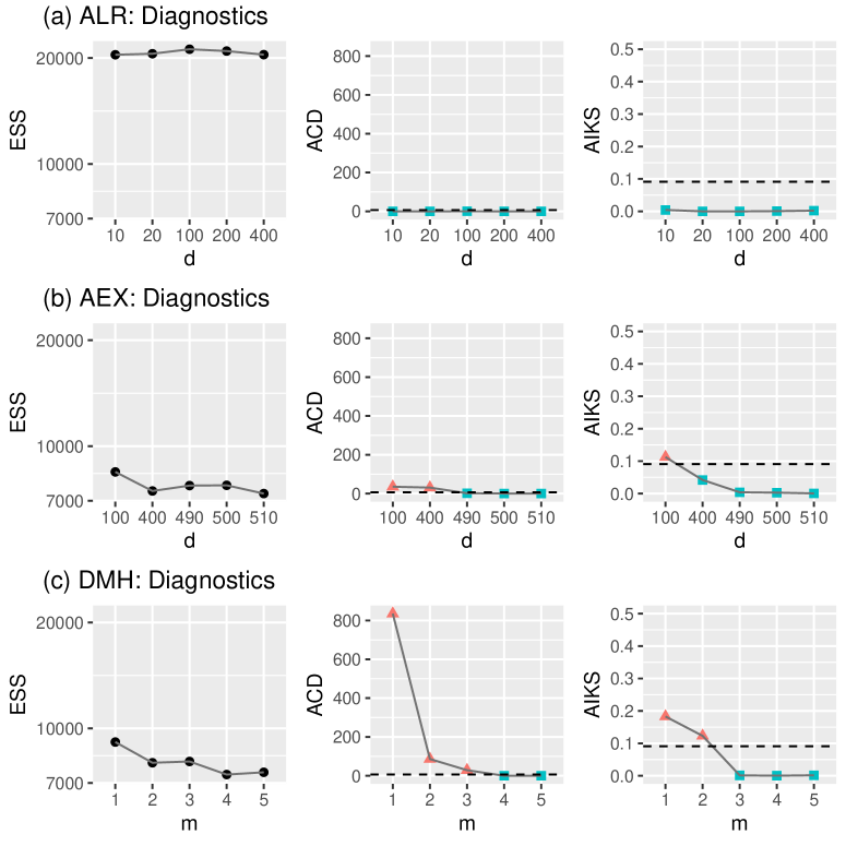
Figure 1: Results for a simulated binary lattice from the Ising model with $\theta=0.2$. (a) Diagnostics (ESS, ACD, and AIKS) applied to samples generated from ALR with different numbers $d$ of particles. (b) Diagnostics applied to samples generated from AEX with different numbers $d$ of particles. (c) Diagnostics applied to samples generated from DMH with different numbers $m$ of (inner) Gibbs updates. A larger ESS is better. For ACD and AIKS, the dashed horizontal lines represent their threshold values, and the red triangles and blue squares indicate poor sample quality and good sample quality, respectively. For ALR, all of the diagnostics are similar for the different values of $d$. For AEX, ESS recommends $d=100$, ACD recommends $d$ of at least 490, and AIKS recommends $d$ of at least 400. For DMH, ESS recommends $m=$ 1, ACD recommends $m$ of 4 or more, and AIKS recommends $m$ of 3 or more.

For this example we consider ALR, AEX, and DMH algorithms that are described in Section 2. The ALR and AEX algorithms are asymptotically exact. The DMH algorithm is asymptotically inexact but was found to be very efficient in terms of effective sample size per unit time and is applicable for doubly intractable problems with higher parameter dimension. To find appropriate values for the tuning parameters of the algorithms, we generate multiple chains from each algorithm with different choices of tuning parameters. We implement AEX with different numbers $d$ of particles, where particles are selected from fractional DMH, which is DMH with a larger acceptance probability. The choice of the other tuning parameters follows Park and Haran, (2018). We implement ALR with different numbers $d$ of particles, where the particles are chosen from a short run of DMH with a single cycle of (inner) Gibbs updates. The choice of other components to be tuned follows Park and Haran, (2018). We implement DMH with different numbers $m$ of (inner) Gibbs updates. We use a uniform prior with range $[0,1]$ for $\theta$.

All algorithms were run for $n$ = 120,000 iterations. For AIKS, in order to make the samples approximately independent, we thinned them at equally spaced intervals of 20, thereby obtaining a sample of size 6,000 having auto-correlation below 0.1. For ACD and AIKS, $N=$ 200,000 auxiliary variables were generated via Gibbs sampling for approximating $\boldsymbol{d}(\boldsymbol{\theta})$ for ACD and $\boldsymbol{u}(\boldsymbol{\theta})$ for AIKS at each unique posterior sample point The posterior sample size $n$ and the auxiliary sample size $N$ were determined by the heuristics stated in Section 4.2 and 5.2 (see Appendix E.1 for details). We used parallel computing to obtain the approximations and to compute AIKS. The threshold value of ACD is the 0.99 quantile of $\chi^{2}(1)$, which is 6.63. For AIKS we estimated the 0.99 quantile of its asymptotic distribution via the bootstrap method for a single sample path and use this threshold value for assessing all samples. The bootstrap procedure took 3.86 minutes and provided 0.08 for the threshold value of AIKS. ACD computation took approximately 5.10 hours and AIKS computation took approximately 1.27 hours.

Table 1: Summary statistics of posterior samples and a gold standard in the Ising model for a simulated binary lattice.

Algorithm	$d$ or $m$	Median	LTP	RTP	Algorithm	$d$ or $m$	Median	LTP	RTP
ALR	10	0.19	0.05	0.05	DMH	1	0.19	0.09	0.09
AEX	490	0.19	0.05	0.05	DMH	4	0.19	0.05	0.05
Gold standard		0.19	0.05	0.05

SD, standard deviation; LTP, left-tail probability; RTP, right-tail probability.

Figure 1 (a) shows the diagnostic values for ALR for various values of $d$. All diagnostics provide the same conclusion: ALR is not so sensitive to the number of particles in this setting. For AEX and DMH, ACD and AIKS provide considerably different conclusions from ESS. In Figure 1 (b) it is observed that ESS is maximised (the best) at $d$ = 100 and generally decreases (worsens) as $d$ increases for AEX. On the other hand, ACD and AIKS have their largest (worst) values at $d=$ 100 and indicate that $d$ should be at least 490 and 400, respectively. Likewise, for DMH, Figure 1 (c) shows that ESS is maximised (the best) at $m$ = 1 and generally decreases (worsens) as $m$ increases, while ACD and AIKS take their largest (worst) values at $m=$ 1 and decrease (improve) as $m$ increases. ACD recommends $m$ of 4 or more and AIKS recommends $m$ of 3 or more.

Table 1 presents summary statistics for some of the posterior samples and a gold standard. We use the sample generated from the exchange algorithm (Murray et al.,, 2006), which is asymptotically exact and has no tuning parameter, as the gold standard. Cutoff values for the left- and right-tail probabilities are the lower 5% and the upper 5% percentiles of the gold standard. Both ACD and AIKS suggest that ALR with $d=$ 10, AEX with $d=$ 490, and DMH with $m=$ 4 provide high quality samples. It is observed that they provide the same values of the summary statistics as the gold standard. ACD and AIKS imply that DMH is computationally much more efficient than the other algorithms and provides samples that are of the same high quality. On the other hand, the ESS-recommended DMH sample with $m=$ 1 does not match the gold standard. It provides higher tail probabilities compared to the gold standard. This shows that ACD and AIKS perform well in assessing how close samples are to the exact posterior. Not surprisingly, ESS is inadequate as a tool for this purpose. In summary, our approaches provide good guidance on how to assess the quality of samples for both the asymptotically exact and asymptotically inexact algorithms. In addition, our diagnostics help one to select the best algorithm and its tuning parameter in terms of computational efficiency.

6.2 A Social Network Model

An exponential family random graph model (ERGM) (Robins et al.,, 2007; Hunter et al.,, 2008) is a statistical model for analysing network data. Consider an undirected ERGM with $n$ vertices. Relationships among the vertices can be represented as an $n\times n$ adjacency matrix $\boldsymbol{x}$ as follows: for all $i\neq j$, $x_{i,j}=1$ if the $i$th and $j$th vertices are connected, and $x_{i,j}=0$ otherwise. And $x_{i,i}$ is 0 for all $i\in\{1,\dots,n\}$, i.e., there are no loops. The number of possible network configurations is $2^{n(n-1)/2}$ and summation over those configurations is required to calculate the normalizing function of the model. Thus computing $c(\boldsymbol{\theta})$ is infeasible unless $n$ is quite small.

For an undirected graph with $n$ vertices, the ERGM likelihood is given by

$$L(\boldsymbol{\theta}\mid\boldsymbol{x}) =\frac{1}{c(\boldsymbol{\theta})}\exp\{\theta_{1}S_{1}(\boldsymbol{x})+\theta_{2}S_{2}(\boldsymbol{x})\},$$

$$S_{1}(\boldsymbol{x}) =\sum_{i=1}^{n}\binom{x_{i+}}{1},$$

$$S_{2}(\boldsymbol{x}) =e^{\tau}\sum_{k=1}^{n-2}\left\{1-(1-e^{-\tau})^{k}\right\}\textup{EP}_{k}(\boldsymbol{x}).$$

The sufficient statistics $S_{1}(\boldsymbol{x})$ and $S_{2}(\boldsymbol{x})$ are the number of edges in the graph and the geometrically weighted edge-wise shared partnership (GWESP) statistic (Hunter and Handcock,, 2006; Hunter,, 2007), respectively. $x_{i+}$ denotes the sum of the $i$th row of the adjacency matrix and $\textup{EP}_{k}(\boldsymbol{x})$ denotes the number of edges between two vertices that share exactly $k$ neighbors. It is assumed that $\tau$ is fixed at a value of 0.25. We simulated a network with 30 actors using 10,000 cycles of Gibbs updates, where the true parameter was $\boldsymbol{\theta}=(\theta_{1},\theta_{2})^{\top}=(-0.96,0.04)^{\top}$.

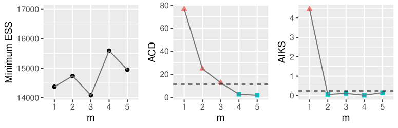
Figure 2: Results for a simulated network from ERGM with $\boldsymbol{\theta}=(\theta_{1},\theta_{2})^{\top}=(-0.96,0.04)^{\top}$. Diagnostics (minimum ESS, ACD, and AIKS) applied to samples generated from DMH with different numbers $m$ of (inner) Gibbs updates. A larger ESS is better. For ACD and AIKS, the dashed horizontal lines represent their threshold values, and the red triangles and blue squares indicate poor sample quality and good sample quality, respectively. The minimum ESS recommends $m$ = 4. ACD recommends $m$ of at least 4 and AIKS recommends $m$ of 2 or more.

For this example we consider the DMH algorithm, which is asymptotically inexact. We explained the DMH algorithm in Section 6.1. We implement DMH with different numbers $m$ of Gibbs updates. We use uniform priors with range $[-5.00,2.27]\times[-1.57,2.32]$ for $(\theta_{1},\theta_{2})^{\top}$, which are centered around the maximum pseudo-likelihood estimates (MPLE) and have widths of 12 standard deviations.

The algorithm was run for 250,000 iterations. For AIKS, in order to make the samples approximately independent, we thinned them at equally spaced intervals of 25 to obtain auto-correlation below 0.1 and a sample of size 10,000. For ACD and AIKS, $N=$ 200,000 auxiliary variables were generated via Gibbs sampling for approximating $\boldsymbol{d}(\boldsymbol{\theta})$ for ACD and $\boldsymbol{u}(\boldsymbol{\theta})$ for AIKS at each unique posterior sample point The posterior sample size $n$ and the auxiliary sample size $N$ were chosen as in the previous example (see Appendix E.2 for details). We used parallel computing to obtain the approximations and to compute AIKS. The threshold value of ACD is the 0.99 quantile of $\chi^{2}(3)$, which is 11.34. For AIKS we estimated the 0.99 quantile of its asymptotic distribution via the bootstrap method, which took 20.99 minutes and provided 0.24. ACD computation took approximately 59.60 hours and AIKS computation took approximately 5.62 hours.

Figure 2 shows the minimum effective sample size, ACD, and AIKS for the DMH sample for a sequence of $m$ values. The minimum ESS is maximised (the best) at $m=$ 4. ACD generally decreases (becomes better) as $m$ increases. ACD implies that $m$ should be at least 4, and AIKS suggests that $m$ should be at least 2. We treat a run from DMH with 20 cycles of Gibbs updates as the gold standard. Both ACD and AIKS indicate good sample quality (ACD = 0.94 and AIKS = 0.01). We observe that all ESS-, ACD-, and AIKS-selected samples provide almost the same values of the summary statistics as the gold standard. In this case, all of the diagnostics generally agree.

6.3 A Conway–Maxwell–Poisson Regression Model

The Conway–Maxwell–Poisson (COMP) distribution (Conway and Maxwell,, 1962) is a two-parameter generalisation of the Poisson distribution for modeling count data that are characterised by under-dispersion (variance less than the mean) or over-dispersion (variance greater than the mean). For a COMP($\lambda$, $\nu$) variable $Y$, the probability mass function is given by

$$P(Y=y) =\frac{1}{c(\lambda,\nu)}\frac{\lambda^{y}}{(y!)^{\nu}},$$

where $\lambda>0$ is a generalisation of the Poisson rate parameter, $\nu\geq 0$ denotes the dispersion parameter, and $c(\lambda,\nu)=\sum_{z=0}^{\infty}\lambda^{z}/(z!)^{\nu}$ is a normalising function. The COMP distribution accommodates under- ($\nu>$ 1), equi- ($\nu=$ 1), or over-dispersion (0 $\leq\nu<$ 1). The COMP distribution forms a continuous bridge between the Poisson ($\nu=$ 1), geometric ($\nu=$ 0 and $\lambda<$ 1), and Bernoulli ($\nu=$ $\infty$ and success probability $\lambda/(1+\lambda)$) distributions. Guikema and Goffelt, (2008) proposed a reparameterisation, substituting $\eta$ = $\lambda^{1/\nu}$ to approximate the center of the COMP distribution. For a count variable $Y$ that follows the COMP_η($\eta$, $\nu$) distribution, the probability mass function is

$$P(Y=y) =\frac{1}{c_{\eta}(\eta,\nu)}\left(\frac{\eta^{y}}{y!}\right)^{\nu},$$

where $c_{\eta}(\eta,\nu)=\sum_{z=0}^{\infty}\left(\eta^{z}/z!\right)^{\nu}$ is the normalising function. Huang, (2017) and Ribeiro et al., (2020) have reparameterised the COMP distribution as a function of the mean. Under any parameterisation, however, the COMP normalising function is an infinite sum, making the function intractable.

For count response variables $Y_{i}$ and corresponding explanatory variables $\boldsymbol{x}_{i}$ $=$ ($x_{i,1}$, $\dots$, $x_{i,p-1}$)^⊤ for $i$ $=$ $1$, $\dots$, $n$, the likelihood of a COMP regression model with log link function for $\eta$ is given by $Y_{i}\sim\text{COMP}_{\eta}(\eta_{i},\nu)$, with $\log(\eta_{i})=\beta_{0}+x_{i,1}\beta_{1}+\cdots+x_{i,p-1}\beta_{p-1}\;(i=1,\dots,n)$, where $\boldsymbol{\beta}$ $=$ ($\beta_{0}$, $\dots$, $\beta_{p-1}$)^⊤ are regression coefficients. We study the takeover bids dataset (Cameron and Johansson,, 1997), which comprises the number of bids received by 126 US firms that were targets of tender offers during the period 1978–1985, along with 9 explanatory variables (see Sáez-Castillo and Conde-Sánchez,, 2013, for details). The dataset can be obtained from mpcmp package (Fung et al.,, 2019). It is assumed that $\nu$ is fixed at a value of 1.754 (Huang,, 2017).

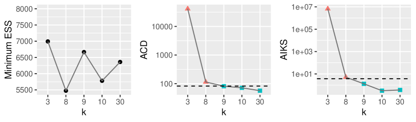
Figure 3: Results for the takeover bids dataset in the COMP regression model. Diagnostics (minimum ESS, ACD, and AIKS) applied to samples generated from NormTrunc with different levels $k$ of truncation. A larger ESS is better. For ACD and AIKS, the dashed horizontal lines represent their threshold values, and the red triangle and blue square imply poor sample quality and good sample quality, respectively. The minimum ESS recommends $k$ = 3. ACD and AIKS recommend $k$ of 9 or more.

For this example we consider a simple and widely used approach, namely, the NormTrunc algorithm. Specifically, we approximate the normalizing function by truncating the infinite sum to a truncation level $k$ such that $c_{\eta}(\eta,\nu)$ $\approx$ $\sum_{z=0}^{k}\left(\eta^{z}/z!\right)^{\nu}$ and use the approximation for each Metropolis–Hastings accept-reject ratio. The NormTrunc algorithm is asymptotically inexact. In order to determine a suitable value of $k$, we implement NormTrunc with different levels $k$ of truncation.

The algorithm was run for 300,000 iterations. For AIKS, in order to make the samples approximately independent, we thinned the samples at equally spaced intervals of 100 to obtain auto-correlation below 0.1 and 3,000 sample points. For ACD and AIKS, $N=$ 200,000 auxiliary variables were generated via Chanialidis et al., (2018)’s rejection sampling algorithm for approximating $\boldsymbol{d}(\boldsymbol{\theta})$ for ACD and $\boldsymbol{u}(\boldsymbol{\theta})$ for AIKS at each unique posterior sample point The posterior sample size $n$ and the auxiliary sample size $N$ were determined as in the previous example (see Appendix E.3 for details). We used parallel computing to obtain the approximations and to compute AIKS. The threshold value of ACD is the 0.99 quantile of $\chi^{2}(55)$, which is 82.29. For AIKS we estimated the 0.99 quantile of its asymptotic distribution via the bootstrap method, which took 9.75 minutes and provided 3.71. ACD computation took approximately 6.29 hours and AIKS computation took approximately 20.71 minutes.

Figure 3 shows minimum effective sample size, ACD, and AIKS for the NormTrunc sample for an array of $k$ values. ACD and AIKS provide considerably different conclusions from ESS. The minimum ESS is maximised (the best) at $k=$ 3. On the other hand, both ACD and AIKS take their largest (worst) values at $k=$ 3 and decrease (improve) as $k$ increases. Both recommend $k$ of 9 or more.

Table 2: Summary statistics of posterior samples and a gold standard for $\beta_{0}$ in the COMP regression model for the takeover bids dataset.

Algorithm	$k$	Median	LTP	RTP	Algorithm	$k$	Median	LTP	RTP
NormTrunc	3	0.45	0.01	0.47	NormTrunc	9	0.31	0.05	0.05
Gold standard		0.31	0.05	0.05

SD, standard deviation; LTP, left-tail probability; RTP, right-tail probability.

Table 2 presents summary statistics for some of the posterior samples and a gold standard. We treat as the gold standard a run from the exchange algorithm (Murray et al.,, 2006), where auxiliary variables are generated by Chanialidis et al., (2018)’s rejection sampling algorithm. Both ACD and AIKS indicate good sample quality (ACD = 70.72 and AIKS = 0.50). The cutoff values for left- and right-tail probabilities and left- and right-center probabilities were chosen as in the previous example. Both ACD and AIKS suggest that NormTrunc with $k=$ 9 provides high quality samples. It is observed that the NormTrunc sample with $k=$ 9 provides the same values of the summary statistics as the gold standard. On the other hand, the ESS-recommended NormTrunc sample with $k=$ 3 does not match the gold standard. It provides a large median and a high right-tail probability compared to the gold standard. In summary, our approaches help tune algorithms. In particular, for asymptotically inexact algorithms, our methods can guide users to appropriately choose their tuning parameters and help provide reliable inference.

6.4 Computational Complexity

We examine the computational complexity of the approximate curvature diagnostic (ACD) and the approximate inverse multiquadric kernel Stein discrepancy (AIKS), summarizing how our diagnostics scale with an increase in the number $n$ of unique posterior sample points and the size $N$ of auxiliary samples.

We denote by $s$ the computational cost of simulating a single auxiliary variable and calculating the derivatives given the auxiliary variable for approximating the intractable terms discussed in Section 4.2. Using $N$ auxiliary variables, we approximate $\boldsymbol{d}(\boldsymbol{\theta})$ for ACD and $\boldsymbol{u}(\boldsymbol{\theta})$ for AIKS at each unique posterior sample point The complexity of the approximation step is $\mathcal{O}(nsN)$. Given the approximations, the complexity for estimating the threshold value of AIKS is $\mathcal{O}(bn^{2})$, where $b$ is the bootstrap sample size. The complexity for ACD is $\mathcal{O}(n)$ and the complexity for AIKS is $\mathcal{O}(n^{2})$, given the approximations. It is important to note that the approximation step and computation of AIKS and its threshold value are embarrassingly parallelizable.

Table 3: Summary statistics for 100 replicates and threshold values of ACD and AIKS in the COMP regression model for the takeover bids dataset.

	ACD					AIKS
$k$	Mean	SD	Min	Max	Threshold value	Mean	SD	Min	Max	Threshold value
8	114.0	0.05	113.9	114.2	82.29	5.138	0.006	5.124	5.151	3.713
9	81.28	0.05	81.17	81.39		1.308	0.002	1.304	1.312

SD, standard deviation

6.5 Variability of Diagnostics

In this section we investigate the variability of ACD and AIKS using the example in Section 6.3. We create 100 replicates of our diagnostics for each posterior sample path. Table 3 shows summary statistics for the replicates. We see that ACD and AIKS have very small standard deviations. Both ACD and AIKS recommend $k$ of at least 9 based on their minimum or maximum values, which shows that they provide the same conclusion across 100 replicates. This implies that the variability of our diagnostic quantities can be controlled by selecting suitable values of tuning parameters; auxiliary sample size $N$ and posterior sample size $n$ for ACD; and auxiliary sample size $N$ for AIKS.

7 Discussion

In this article we proposed new methods that provide guidance for tuning algorithms and give some measure of sample quality for a wide range of Monte Carlo algorithms, including a particularly challenging class of algorithms: asymptotically inexact algorithms for distributions with intractable normalizing functions. We describe three methods. CD applies broadly to most any likelihood-based context where misspecification is of concern while ACD and AIKS are specifically targeted at likelihoods with intractable normalizing functions. Our study mainly focuses on intractable normalizing function problems and shows that our methods can assess the quality of samples and provide good guidance for tuning algorithms. We have studied applications of ACD and AIKS to several asymptotically exact and inexact algorithms in the context of challenging simulated and real data examples. This shows that our methods provide useful results not only for asymptotically exact algorithms, for which some other methods may be useful, but also for asymptotically inexact algorithms, for which we are not aware of other methods.

There are of course simple and reasonable heuristics one can use for diagnostic purposes, such as increasing $m$ until DMH approximations stabilize. However, our diagnostics go beyond simple approaches, allowing one to compare sample quality across different algorithms, including comparing asymptotically exact algorithms with asymptotically inexact algorithms.

We note that ACD and AIKS could be slightly different in their conclusions, as our examples illustrate, but the difference is quite small and conclusions are nearly the same overall. For auto-correlated samples, as in our examples, ACD uses the entire sample path while AIKS employs a thinned sample. The difference between ACD and AIKS also stems from the fact that they consider different sets of test functions to quantify the difference between a sample mean and a target expectation. ACD considers two functions whose target expectations are identical and measures the difference between sample means of the two functions. AIKS considers a set of functions whose target expectations are zero and finds the maximum error between the sample mean and the target expectation. Unless the score function of the target density is the origin, their sets of test functions are mutually exclusive, which is the case of all the examples in this article. Depending on the setting, one of ACD or AIKS may be more useful than the other. ACD is applicable to both independent and Markovian sample paths, whereas AIKS is only applicable to independent samples. To use AIKS for Markovian sample paths, we may thin the samples such that auto-correlation is sufficiently reduced. However, one advantage of AIKS is that it does not require a large posterior sample size $n$, performing reliably for $n$ = 1,000 and being computationally efficient (Liu et al.,, 2016). Additionally AIKS is supported by a theory of weak convergence and thus can be used for deciding convergence of a sequence of sample points to the target distribution.

ACD and AIKS are obtained by replacing some functions that have to be evaluated for CD and IMQ KSD with their Monte Carlo approximations. This allows for the diagnostics to be available for doubly intractable posterior distributions. The computing time of ACD and AIKS mainly accounts for the Monte Carlo approximation, which might be computationally expensive for high-dimensional datasets. However, the approximation step is embarrassingly parallel in that the Monte Carlo estimates at the posterior sample points can be constructed entirely in parallel. Therefore, the computational expense can be decreased by a factor corresponding to the number of available cores. This can be helpful provided that the availability of parallel computing resources increases. An important caveat of ACD is that it can be misled if the first two moments match the target distribution but higher order moments do not. AIKS cannot be misled in such fashion. Developing fast approaches for obtaining the approximations and extending ACD to higher order moments may provide interesting avenues for future research.

Appendix A Monte Carlo approximations to intractable terms

A.1 Derivative of log normalizing function

For a $p$-dimensional parameter vector $\boldsymbol{\theta}$, consider a posterior density $\pi(\boldsymbol{\theta}\mid\boldsymbol{x})$ whose likelihood function is $L(\boldsymbol{\theta}\mid\boldsymbol{x})=h(\boldsymbol{x}\mid\boldsymbol{\theta})/c(\boldsymbol{\theta})$ and prior density is $p(\boldsymbol{\theta})$. The $k$th entry of $\nabla_{\boldsymbol{\theta}}\log c(\boldsymbol{\theta}\mid\boldsymbol{x})$, the score function of the normalizing function, can be written as

$$\frac{\partial\log c(\boldsymbol{\theta})}{\partial\theta_{k}} =\frac{1}{c(\boldsymbol{\theta})}\frac{\partial c(\boldsymbol{\theta})}{\partial\theta_{k}}$$

$$=\frac{1}{c(\boldsymbol{\theta})}\frac{\partial}{\partial\theta_{k}}\int_{\boldsymbol{\mathcal{X}}}h(\boldsymbol{x}|\boldsymbol{\theta})d\boldsymbol{x}$$

$$=\frac{1}{c(\boldsymbol{\theta})}\int_{\boldsymbol{\mathcal{X}}}\frac{\partial h(\boldsymbol{x}|\boldsymbol{\theta})}{\partial\theta_{k}}d\boldsymbol{x}$$ (4)

$$=\frac{1}{c(\boldsymbol{\theta})}\int_{\boldsymbol{\mathcal{X}}}h(\boldsymbol{x}|\boldsymbol{\theta})\frac{\partial\log h(\boldsymbol{x}|\boldsymbol{\theta})}{\partial\theta_{k}}d\boldsymbol{x}$$

$$=\int_{\boldsymbol{\mathcal{X}}}\frac{\partial\log h(\boldsymbol{x}|\boldsymbol{\theta})}{\partial\theta_{k}}f(\boldsymbol{x}|\boldsymbol{\theta})d\boldsymbol{x}$$

$$=\textup{E}_{f}\left\{\frac{\partial\log h(\boldsymbol{X}|\boldsymbol{\theta})}{\partial\theta_{k}}\right\}.$$ (5)

Equation (4) follows from the dominated convergence theorem. Under the assumptions that the score function exists and the score function and the normalizing function are bounded, we have exchanged the derivative with the integral.

A.2 Second derivative of log normalizing function

The $(k,l)$th entry of $\frac{\partial}{\partial\boldsymbol{\theta}}\nabla_{\boldsymbol{\theta}}\log c(\boldsymbol{\theta}\mid\boldsymbol{x})$, the Hessian matrix of the normalizing function, is given by

$$\frac{\partial^{2}\log c(\boldsymbol{\theta})}{\partial\theta_{k}\partial\theta_{l}} =\frac{\partial}{\partial\theta_{k}}\left\{\frac{1}{c(\boldsymbol{\theta})}\frac{\partial c(\boldsymbol{\theta})}{\partial\theta_{l}}\right\}$$

$$=\frac{1}{c(\boldsymbol{\theta})}\frac{\partial^{2}c(\boldsymbol{\theta})}{\partial\theta_{k}\partial\theta_{l}}-\left\{\frac{1}{c(\boldsymbol{\theta})}\frac{\partial c(\boldsymbol{\theta})}{\partial\theta_{k}}\right\}\left\{\frac{1}{c(\boldsymbol{\theta})}\frac{\partial c(\boldsymbol{\theta})}{\partial\theta_{l}}\right\}$$

$$=\frac{1}{c(\boldsymbol{\theta})}\frac{\partial^{2}c(\boldsymbol{\theta})}{\partial\theta_{k}\partial\theta_{l}}-\textup{E}_{f}\left\{\frac{\partial\log h(\boldsymbol{X}|\boldsymbol{\theta})}{\partial\theta_{k}}\right\}\textup{E}_{f}\left\{\frac{\partial\log h(\boldsymbol{X}|\boldsymbol{\theta})}{\partial\theta_{l}}\right\}.$$ (6)

Now consider the first term on the right hand side of equation (6). It can be written as

$$\frac{1}{c(\boldsymbol{\theta})}\frac{\partial^{2}c(\boldsymbol{\theta})}{\partial\theta_{k}\partial\theta_{l}} =\frac{1}{c(\boldsymbol{\theta})}\frac{\partial^{2}}{\partial\theta_{k}\partial\theta_{l}}\int_{\boldsymbol{\mathcal{X}}}h(\boldsymbol{x}|\boldsymbol{\theta})d\boldsymbol{x}$$

$$=\frac{1}{c(\boldsymbol{\theta})}\int_{\boldsymbol{\mathcal{X}}}\frac{\partial}{\partial\theta_{k}}\left\{\frac{\partial\log h(\boldsymbol{x}|\boldsymbol{\theta})}{\partial\theta_{l}}h(\boldsymbol{x}|\boldsymbol{\theta})\right\}d\boldsymbol{x}$$ (7)

$$=\int_{\boldsymbol{\mathcal{X}}}\frac{\partial^{2}\log h(\boldsymbol{x}|\boldsymbol{\theta})}{\partial\theta_{k}\partial\theta_{l}}f(\boldsymbol{x}|\boldsymbol{\theta})d\boldsymbol{x}+\int_{\boldsymbol{\mathcal{X}}}\frac{\partial\log h(\boldsymbol{x}|\boldsymbol{\theta})}{\partial\theta_{k}}\frac{\partial\log h(\boldsymbol{x}|\boldsymbol{\theta})}{\partial\theta_{l}}f(\boldsymbol{x}|\boldsymbol{\theta})d\boldsymbol{x}$$

$$=\textup{E}_{f}\left\{\frac{\partial^{2}\log h(\boldsymbol{X}|\boldsymbol{\theta})}{\partial\theta_{k}\partial\theta_{l}}\right\}+\textup{E}_{f}\left\{\frac{\partial\log h(\boldsymbol{X}|\boldsymbol{\theta})}{\partial\theta_{k}}\frac{\partial\log h(\boldsymbol{X}|\boldsymbol{\theta})}{\partial\theta_{l}}\right\}.$$ (8)

In the equation (7) we have exchanged the derivative with the integral, owing to the dominated convergence theorem. Combining (6) and (8), the entry of $\frac{\partial}{\partial\boldsymbol{\theta}}\nabla_{\boldsymbol{\theta}}\log c(\boldsymbol{\theta}\mid\boldsymbol{x})$ is

$$\frac{\partial^{2}\log c(\boldsymbol{\theta})}{\partial\theta_{k}\partial\theta_{l}} =\textup{E}_{f}\left\{\frac{\partial^{2}\log h(\boldsymbol{X}|\boldsymbol{\theta})}{\partial\theta_{k}\partial\theta_{l}}\right\}+\textup{E}_{f}\left\{\frac{\partial\log h(\boldsymbol{X}|\boldsymbol{\theta})}{\partial\theta_{k}}\frac{\partial\log h(\boldsymbol{X}|\boldsymbol{\theta})}{\partial\theta_{l}}\right\}$$

$$-\textup{E}_{f}\left\{\frac{\partial\log h(\boldsymbol{X}|\boldsymbol{\theta})}{\partial\theta_{k}}\right\}\textup{E}_{f}\left\{\frac{\partial\log h(\boldsymbol{X}|\boldsymbol{\theta})}{\partial\theta_{l}}\right\}.$$ (9)

A.3 Monte Carlo approximations

We approximate the $k$th entry of the vector $\nabla_{\boldsymbol{\theta}}\log c(\boldsymbol{\theta})$ using a sample generated from the model distribution:

$$\frac{\partial\log c(\boldsymbol{\theta})}{\partial\theta_{k}} \approx\frac{1}{N}\sum_{j=1}^{N}\frac{\partial\log h(\boldsymbol{y}^{(j)}|\boldsymbol{\theta})}{\partial\theta_{k}},$$

where $\boldsymbol{y}^{(1)},\dots,\boldsymbol{y}^{(N)}$ are auxiliary variables generated exactly from $f(\cdot\mid\boldsymbol{\theta})$ or generated by a Monte Carlo algorithm having $f(\cdot\mid\boldsymbol{\theta})$ as its target distribution. In a similar fashion, the approximation of the $(k,l)$th entry of $\left\{\nabla_{\boldsymbol{\theta}}\log c(\boldsymbol{\theta})\right\}$ $\left\{\nabla_{\boldsymbol{\theta}}\log c(\boldsymbol{\theta})\right\}^{\top}$ is calculated as

$$\frac{\partial\log c(\boldsymbol{\theta})}{\partial\theta_{k}}\frac{\partial\log c(\boldsymbol{\theta})}{\partial\theta_{l}} \approx\left\{\frac{1}{N}\sum_{j=1}^{N}\frac{\partial\log h(\boldsymbol{y}^{(j)}|\boldsymbol{\theta})}{\partial\theta_{k}}\right\}\left\{\frac{1}{N}\sum_{j=1}^{N}\frac{\partial\log h(\boldsymbol{y}^{(j)}|\boldsymbol{\theta})}{\partial\theta_{l}}\right\},\;k,l=1,\dots,p.$$

Lastly we approximate $(k,l)$th entry of $\frac{\partial}{\partial\boldsymbol{\theta}}\nabla_{\boldsymbol{\theta}}\log c(\boldsymbol{\theta})$ by

$$\frac{\partial^{2}\log c(\boldsymbol{\theta})}{\partial\theta_{k}\theta_{l}} \approx\frac{1}{N}\sum_{j=1}^{N}\frac{\partial^{2}\log h(\boldsymbol{y}^{(j)}|\boldsymbol{\theta})}{\partial\theta_{k}\partial\theta_{l}}+\frac{1}{N}\sum_{j=1}^{N}\frac{\partial\log h(\boldsymbol{y}^{(j)}|\boldsymbol{\theta})}{\partial\theta_{k}}\frac{\partial\log h(\boldsymbol{y}^{(j)}|\boldsymbol{\theta})}{\partial\theta_{l}}$$

$$-\left\{\frac{1}{N}\sum_{j=1}^{N}\frac{\partial\log h(\boldsymbol{y}^{(j)}|\boldsymbol{\theta})}{\partial\theta_{k}}\right\}\left\{\frac{1}{N}\sum_{j=1}^{N}\frac{\partial\log h(\boldsymbol{y}^{(j)}|\boldsymbol{\theta})}{\partial\theta_{l}}\right\}.$$

Appendix B Proof of Theorem 1

Let $D(\boldsymbol{\theta})=J(\boldsymbol{\theta})+H(\boldsymbol{\theta})$ and $D_{k,l}(\boldsymbol{\theta})$ be the $(k,l)$ entry of $D(\boldsymbol{\theta})$. Let $\hat{D}_{k,l}(\boldsymbol{\theta})$ be the approximation, computed using auxiliary variables $\boldsymbol{y}^{(1)}$,…,$\boldsymbol{y}^{(N)}$ generated from the model distribution, to $D_{k,l}(\boldsymbol{\theta})$. Suppose we have an i.i.d. sample $\boldsymbol{\theta}^{(1)},\dots,\boldsymbol{\theta}^{(n)}$ generated from $\pi(\cdot\mid\boldsymbol{x})$. For all $k,l,m,s\in\{1,\dots,p\}$, the difference between an entry of $V=\textup{E}_{\pi}\{\boldsymbol{d}(\boldsymbol{\theta})\boldsymbol{d}(\boldsymbol{\theta})^{\top}\}$ and its two-state approximation is

$$\left|\textup{E}_{\pi}\{D_{k,l}(\boldsymbol{\theta})D_{m,s}(\boldsymbol{\theta})\}-\frac{1}{n}\sum_{i=1}^{n}\hat{D}_{k,l}(\boldsymbol{\theta}^{(i)})\hat{D}_{m,s}(\boldsymbol{\theta}^{(i)})\right|$$

$$\leq\left|\frac{1}{n}\sum_{i=1}^{n}D_{k,l}(\boldsymbol{\theta}^{(i)})D_{m,s}(\boldsymbol{\theta}^{(i)})-\textup{E}_{\pi}\{D_{k,l}(\boldsymbol{\theta})D_{m,s}(\boldsymbol{\theta})\}\right|$$

$$\quad+\left|\frac{1}{n}\sum_{i=1}^{n}\left\{\hat{D}_{k,l}(\boldsymbol{\theta}^{(i)})\hat{D}_{m,s}(\boldsymbol{\theta}^{(i)})-D_{k,l}(\boldsymbol{\theta}^{(i)})D_{m,s}(\boldsymbol{\theta}^{(i)})\right\}\right|$$

$$\leq\delta(n)+\frac{1}{n}\sum_{i=1}^{n}\left|\hat{D}_{k,l}(\boldsymbol{\theta}^{(i)})\hat{D}_{m,s}(\boldsymbol{\theta}^{(i)})-D_{k,l}(\boldsymbol{\theta}^{(i)})D_{m,s}(\boldsymbol{\theta}^{(i)})\right|,$$ (10)

where $\delta(n)=\|\frac{1}{n}\sum_{i=1}^{n}\boldsymbol{d}(\boldsymbol{\theta}^{(i)})\boldsymbol{d}(\boldsymbol{\theta}^{(i)})^{\top}-\textup{E}_{\pi}\{\boldsymbol{d}(\boldsymbol{\theta})\boldsymbol{d}(\boldsymbol{\theta})^{\top}\}\|_{\max}=\mathcal{O}(n^{-1/2})$ from the ergodic theorem. Now we consider the second term on the right hand side of inequality (10). Let $u_{k}(\boldsymbol{\theta})$ be the $k$th entry of the score function $\boldsymbol{u}(\boldsymbol{\theta})$ of the posterior distribution and $\hat{u}_{k}(\boldsymbol{\theta})$ be its approximation computed using the auxiliary variables. Let $H_{k,l}(\boldsymbol{\theta})$ be the $(k,l)$th entry of the hessian matrix $H(\boldsymbol{\theta})$ of the posterior distribution and $\hat{H}_{k,l}(\boldsymbol{\theta})$ be its approximation computed using the auxiliary variables. We can bound the difference between $\hat{D}_{k,l}(\boldsymbol{\theta})\hat{D}_{m,s}(\boldsymbol{\theta})$ and $D_{k,l}(\boldsymbol{\theta})D_{m,s}(\boldsymbol{\theta})$ as follows. For all $k,l,m,s\in\{1,\dots,p\}$, we have

$$\left|\hat{D}_{k,l}(\boldsymbol{\theta})\hat{D}_{m,s}(\boldsymbol{\theta})-D_{k,l}(\boldsymbol{\theta})D_{m,s}(\boldsymbol{\theta})\right| \leq\left|\hat{u}_{k}(\boldsymbol{\theta})\hat{u}_{l}(\boldsymbol{\theta})\hat{u}_{m}(\boldsymbol{\theta})\hat{u}_{s}(\boldsymbol{\theta})-u_{k}(\boldsymbol{\theta})u_{l}(\boldsymbol{\theta})u_{m}(\boldsymbol{\theta})u_{s}(\boldsymbol{\theta})\right|$$

$$\quad+\left|\hat{u}_{k}(\boldsymbol{\theta})\hat{u}_{l}(\boldsymbol{\theta})\hat{H}_{m,s}(\boldsymbol{\theta})-u_{k}(\boldsymbol{\theta})u_{l}(\boldsymbol{\theta})H_{m,s}(\boldsymbol{\theta})\right|$$

$$\quad+\left|\hat{u}_{m}(\boldsymbol{\theta})\hat{u}_{s}(\boldsymbol{\theta})\hat{H}_{k,l}(\boldsymbol{\theta})-u_{m}(\boldsymbol{\theta})u_{s}(\boldsymbol{\theta})H_{k,l}(\boldsymbol{\theta})\right|$$

$$\quad+\left|\hat{H}_{k,l}(\boldsymbol{\theta})\hat{H}_{m,s}(\boldsymbol{\theta})-H_{k,l}(\boldsymbol{\theta})H_{m,s}(\boldsymbol{\theta})\right|.$$ (11)

Let

$$\epsilon_{1}(N) =\max_{k}\left|\frac{1}{N}\sum_{j=1}^{N}\frac{\partial\log h(\boldsymbol{y}^{(j)}|\boldsymbol{\theta})}{\partial\theta_{k}}-\textup{E}_{f}\left\{\frac{\partial\log h(\boldsymbol{X}|\boldsymbol{\theta})}{\partial\theta_{k}}\right\}\right|,$$

$$\epsilon_{2}(N) =\max_{k,l}\left|\frac{1}{N}\sum_{j=1}^{N}\frac{\partial^{2}\log h(\boldsymbol{y}^{(j)}|\boldsymbol{\theta})}{\partial\theta_{k}\partial\theta_{l}}-\textup{E}_{f}\left\{\frac{\partial^{2}\log h(\boldsymbol{X}|\boldsymbol{\theta})}{\partial\theta_{k}\partial\theta_{l}}\right\}\right|,$$

$$\epsilon_{3}(N) =\max_{l}\left|\frac{1}{N}\sum_{j=1}^{N}\frac{\partial^{3}\log h(\boldsymbol{y}^{(j)}|\boldsymbol{\theta})}{\partial\theta_{k}\partial\theta_{l}\partial\theta_{m}}-\textup{E}_{f}\left\{\frac{\partial^{3}\log h(\boldsymbol{X}|\boldsymbol{\theta})}{\partial\theta_{k}\partial\theta_{l}\partial\theta_{m}}\right\}\right|,$$

$$\epsilon_{4}(N) =\max_{k,l}\left|\frac{1}{N}\sum_{j=1}^{N}\left\{\frac{\partial\log h(\boldsymbol{y}^{(j)}|\boldsymbol{\theta})}{\partial\theta_{k}}\right\}\left\{\frac{\partial\log h(\boldsymbol{y}^{(j)}|\boldsymbol{\theta})}{\partial\theta_{l}}\right\}-\textup{E}_{f}\left\{\frac{\partial\log h(\boldsymbol{X}|\boldsymbol{\theta})}{\partial\theta_{k}}\frac{\partial\log h(\boldsymbol{X}|\boldsymbol{\theta})}{\partial\theta_{l}}\right\}\right|,$$

$$\epsilon_{5}(N) =\max_{k,l,m}\left|\frac{1}{N}\sum_{j=1}^{N}\left\{\frac{\partial\log h(\boldsymbol{y}^{(j)}|\boldsymbol{\theta})}{\partial\theta_{k}}\right\}\left\{\frac{\partial^{2}\log h(\boldsymbol{y}^{(j)}|\boldsymbol{\theta})}{\partial\theta_{l}\partial\theta_{m}}\right\}-\textup{E}_{f}\left\{\frac{\partial\log h(\boldsymbol{X}|\boldsymbol{\theta})}{\partial\theta_{k}}\frac{\partial^{2}\log h(\boldsymbol{X}|\boldsymbol{\theta})}{\partial\theta_{l}\partial\theta_{m}}\right\}\right|,$$

$$\epsilon_{6}(N) =\max_{k,l,m}\Bigg{|}\frac{1}{N}\sum_{j=1}^{N}\left\{\frac{\partial\log h(\boldsymbol{y}^{(j)}|\boldsymbol{\theta})}{\partial\theta_{k}}\right\}\left\{\frac{\partial\log h(\boldsymbol{y}^{(j)}|\boldsymbol{\theta})}{\partial\theta_{l}}\right\}\left\{\frac{\partial\log h(\boldsymbol{y}^{(j)}|\boldsymbol{\theta})}{\partial\theta_{m}}\right\}$$

$$\qquad\qquad-\textup{E}_{f}\left\{\frac{\partial\log h(\boldsymbol{X}|\boldsymbol{\theta})}{\partial\theta_{k}}\frac{\partial\log h(\boldsymbol{X}|\boldsymbol{\theta})}{\partial\theta_{l}}\frac{\partial\log h(\boldsymbol{X}|\boldsymbol{\theta})}{\partial\theta_{m}}\right\}\Bigg{|},$$

and $\epsilon(N)=\max\left\{\epsilon_{1}(N),\epsilon_{2}(N),\epsilon_{3}(N),\epsilon_{4}(N),\epsilon_{5}(N),\epsilon_{6}(N)\right\}$ = $\mathcal{O}(N^{-1/2})$ from the ergodic theorem. Now consider the first term on the right hand side of inequality (11). For all $k,l,m,s\in\{1,\dots,p\}$, we have

$$\left|\hat{u}_{k}(\boldsymbol{\theta})\hat{u}_{l}(\boldsymbol{\theta})\hat{u}_{m}(\boldsymbol{\theta})\hat{u}_{s}(\boldsymbol{\theta})-u_{k}(\boldsymbol{\theta})u_{l}(\boldsymbol{\theta})u_{m}(\boldsymbol{\theta})u_{s}(\boldsymbol{\theta})\right|$$

$$\leq\left\{4(c_{p}^{\prime}+c_{h}^{\prime})^{3}+12c_{h}^{\prime}(c_{p}^{\prime}+c_{h}^{\prime})^{2}+12c_{h}^{\prime 2}(c_{p}^{\prime}+c_{h}^{\prime})+4c_{h}^{\prime 3}\right\}\epsilon(N),$$

which follows from Assumptions 1 and 2, and the following elementary inequalities:

$$|ab-\hat{a}\hat{b}| =|ab-\hat{a}b+\hat{a}b-\hat{a}\hat{b}|=|(a-\hat{a})b+(b-\hat{b})\hat{a}|$$

$$\leq|a-\hat{a}||b|+|b-\hat{b}||\hat{a}|,$$ (13)

$$|abc-\hat{a}\hat{b}\hat{c}| =|abc-\hat{a}bc+\hat{a}bc-\hat{a}\hat{b}\hat{c}|=|(a-\hat{a})bc+(bc-\hat{b}\hat{c})\hat{a}|$$

$$\leq|a-\hat{a}||b||c|+|bc-\hat{b}\hat{c}||\hat{a}|,$$ (14)

$$|abcd-\hat{a}\hat{b}\hat{c}\hat{d}| =|abcd-\hat{a}bcd+\hat{a}bcd-\hat{a}\hat{b}\hat{c}\hat{d}|=|(a-\hat{a})bcd+(bcd-\hat{b}\hat{c}\hat{d})\hat{a}|$$

$$\leq|a-\hat{a}||b||c||d|+|bcd-\hat{b}\hat{c}\hat{d}||\hat{a}|.$$ (15)

Now consider the remaining terms on the right hand side of inequality (11). In a similar fashion, for all $k,l,m,s\in\{1,\dots,p\}$, we have

$$\left|\hat{u}_{k}(\boldsymbol{\theta})\hat{u}_{l}(\boldsymbol{\theta})\hat{H}_{m,s}(\boldsymbol{\theta})-u_{k}(\boldsymbol{\theta})u_{l}(\boldsymbol{\theta})H_{m,s}(\boldsymbol{\theta})\right|$$

$$\leq\left\{(8c_{h}^{\prime}+6c_{h}^{\prime 2})(c_{p}^{\prime}+c_{h}^{\prime})+2(1+c_{h}^{\prime})(c_{p}^{\prime}+c_{h}^{\prime})^{2}+(2c_{p}^{\prime}+4c_{h}^{\prime})(c_{p}^{\prime\prime}+c_{h}^{\prime\prime})+6c_{h}^{\prime\prime}+4c_{h}^{\prime\prime}\right\}\epsilon(N),$$

$$\left|\hat{u}_{m}(\boldsymbol{\theta})\hat{u}_{s}(\boldsymbol{\theta})\hat{H}_{k,l}(\boldsymbol{\theta})-u_{m}(\boldsymbol{\theta})u_{s}(\boldsymbol{\theta})H_{k,l}(\boldsymbol{\theta})\right|$$

$$\leq\left\{(8c_{h}^{\prime}+6c_{h}^{\prime 2})(c_{p}^{\prime}+c_{h}^{\prime})+2(1+c_{h}^{\prime})(c_{p}^{\prime}+c_{h}^{\prime})^{2}+(2c_{p}^{\prime}+4c_{h}^{\prime})(c_{p}^{\prime\prime}+c_{h}^{\prime\prime})+6c_{h}^{\prime\prime}+4c_{h}^{\prime\prime}\right\}\epsilon(N),$$

and

$$|\hat{H}_{k,l}(\boldsymbol{\theta})\hat{H}_{m,s}(\boldsymbol{\theta})-H_{k,l}(\boldsymbol{\theta})H_{m,s}(\boldsymbol{\theta})|\leq\left\{4(c_{p}^{\prime\prime}+c_{h}^{\prime\prime})+4c_{h}^{\prime}(c_{p}^{\prime\prime}+c_{h}^{\prime\prime})+8c_{h}^{\prime}+12c_{h}^{\prime 2}+4c_{h}^{\prime 3}\right\}\epsilon(N).$$

These inequalities follow from Assumptions 1 and 2 in the manuscript and inequalities (13) to (15). Therefore, the approximation error of the two-stage approximation to the asymptotic covariance matrix is

$$\|\hat{V}_{n,N}-V\|_{\max} \leq\mathcal{O}\left(n^{-1/2}\right)+\mathcal{O}\left(N^{-1/2}\right),$$

almost surely. We use $\|\cdot\|_{\max}$ to represent the max norm of vectors or matrices.

Appendix C Proof of Theorem 2

Suppose we have a sample $\boldsymbol{\theta}^{(1)},\dots,\boldsymbol{\theta}^{(n)}$ generated from a polynomially ergodic Markov chain with $\pi(\boldsymbol{\theta}\mid\boldsymbol{x})$ as its stationary distribution. Let $D(\boldsymbol{\theta})=J(\boldsymbol{\theta})+H(\boldsymbol{\theta})$ and $\hat{D}(\boldsymbol{\theta})$ be the approximation, computed using auxiliary variables $\boldsymbol{y}^{(1)}$,…,$\boldsymbol{y}^{(N)}$ generated from the model distribution, to $D(\boldsymbol{\theta})$. Let $\bar{D}=\frac{1}{n}\sum_{i=1}^{n}D(\boldsymbol{\theta}^{(i)})$, $\hat{\bar{D}}=\frac{1}{n}\sum_{i=1}^{n}\hat{D}(\boldsymbol{\theta}^{(i)})$, $\bar{D}^{j}=\frac{1}{b_{n}}\sum_{i=(j-1)b_{n}+1}^{jb_{n}}D(\boldsymbol{\theta}^{(i)})$, and $\hat{\bar{D}}^{j}=\frac{1}{b_{n}}\sum_{i=(j-1)b_{n}+1}^{jb_{n}}\hat{D}(\boldsymbol{\theta}^{(i)})$ for $j=1,\dots,a_{n}$, where $a_{n}$ is the number of batches and $b_{n}$ is the batch size. For all $k,l,m,s\in\{1,\dots,p\}$, the difference between an entry $\sigma_{r}$ of $\Sigma$ and its two-state batch means approximation is

$$\left|\sigma_{r}-\frac{b_{n}}{a_{n}-1}\sum_{j=1}^{a_{n}}(\hat{\bar{D}}^{j}_{k,l}-\hat{\bar{D}}_{k,l})(\hat{\bar{D}}^{j}_{m,s}-\hat{\bar{D}}_{m,s})\right|$$

$$\leq\left|\frac{b_{n}}{a_{n}-1}\sum_{j=1}^{a_{n}}(\bar{D}^{j}_{k,l}-\bar{D}_{k,l})(\bar{D}^{j}_{m,s}-\bar{D}_{m,s})-\sigma_{r}\right|$$

$$\quad+\left|\frac{b_{n}}{a_{n}-1}\sum_{j=1}^{a_{n}}\left\{(\hat{\bar{D}}^{j}_{k,l}-\hat{\bar{D}}_{k,l})(\hat{\bar{D}}^{j}_{m,s}-\hat{\bar{D}}_{m,s})-(\bar{D}^{j}_{k,l}-\bar{D}_{k,l})(\bar{D}^{j}_{m,s}-\bar{D}_{m,s})\right\}\right|$$

$$\leq\gamma(n)+\frac{b_{n}}{a_{n}-1}\sum_{j=1}^{a_{n}}\left|(\hat{\bar{D}}^{j}_{k,l}-\hat{\bar{D}}_{k,l})(\hat{\bar{D}}^{j}_{m,s}-\hat{\bar{D}}_{m,s})-(\bar{D}^{j}_{k,l}-\bar{D}_{k,l})(\bar{D}^{j}_{m,s}-\bar{D}_{m,s})\right|,$$ (16)

where $\gamma(n)=\|\hat{\Sigma}_{n}-\Sigma\|_{\max}=\mathcal{O}\left((\log n/b_{n})^{1/2}n^{1/2-\lambda}\right)\to 0$ as $n\to\infty$ for some $\lambda>0$ under some conditions (Theorem 2 in Vats et al.,, 2019). Now we consider the second term on the right hand side of inequality (16). For all $k,l,m,s\in\{1,\dots,p\}$, we have

$$b_{n}\left|(\hat{\bar{D}}^{j}_{k,l}-\hat{\bar{D}}_{k,l})(\hat{\bar{D}}^{j}_{m,s}-\hat{\bar{D}}_{m,s})-(\bar{D}^{j}_{k,l}-\bar{D}_{k,l})(\bar{D}^{j}_{m,s}-\bar{D}_{m,s})\right|$$

$$=\left|b_{n}^{1/2}(\hat{\bar{D}}^{j}_{k,l}-\hat{\bar{D}}_{k,l})b_{n}^{1/2}(\hat{\bar{D}}^{j}_{m,s}-\hat{\bar{D}}_{m,s})-b_{n}^{1/2}(\bar{D}^{j}_{k,l}-\bar{D}_{k,l})b_{n}^{1/2}(\bar{D}^{j}_{m,s}-\bar{D}_{m,s})\right|$$

$$\leq\left|b_{n}^{1/2}(\bar{D}^{j}_{k,l}-\bar{D}_{k,l})-b_{n}^{1/2}(\hat{\bar{D}}^{j}_{k,l}-\hat{\bar{D}}_{k,l})\right|\left|b_{n}^{1/2}(\bar{D}^{j}_{m,s}-\bar{D}_{m,s})\right|$$

$$\quad+\left|b_{n}^{1/2}(\bar{D}^{j}_{m,s}-\bar{D}_{m,s})-b_{n}^{1/2}(\hat{\bar{D}}^{j}_{m,s}-\hat{\bar{D}}_{m,s})\right|\left|b_{n}^{1/2}(\hat{\bar{D}}^{j}_{k,l}-\hat{\bar{D}}_{k,l})\right|$$ (17)

$$\leq\left|b_{n}^{1/2}(\bar{D}^{j}_{k,l}-\hat{\bar{D}}^{j}_{k,l})-b_{n}^{1/2}(\bar{D}_{k,l}-\hat{\bar{D}}_{k,l})\right|$$

$$\quad\times\left|b_{n}^{1/2}\left\{\bar{D}^{j}_{m,s}-\textup{E}_{\pi}[D_{m,s}(\boldsymbol{\theta})]\right\}-b_{n}^{1/2}\left\{\bar{D}_{m,s}-\textup{E}_{\pi}[D_{m,s}(\boldsymbol{\theta})]\right\}\right|$$

$$\quad+\left|b_{n}^{1/2}(\bar{D}^{j}_{m,s}-\hat{\bar{D}}^{j}_{m,s})-b_{n}^{1/2}(\bar{D}_{m,s}-\hat{\bar{D}}_{m,s})\right|$$

$$\quad\times\left|b_{n}^{1/2}(\hat{\bar{D}}^{j}_{k,l}-\bar{D}^{j}_{k,l})-b_{n}^{1/2}(\hat{\bar{D}}_{k,l}-\bar{D}_{k,l})+b_{n}^{1/2}\left\{\bar{D}^{j}_{k,l}-\textup{E}_{\pi}[D_{k,l}(\boldsymbol{\theta})]\right\}-b_{n}^{1/2}\left\{\bar{D}_{k,l}-\textup{E}_{\pi}[D_{k,l}(\boldsymbol{\theta})]\right\}\right|$$

$$\leq\left\{b_{n}^{1/2}|\bar{D}^{j}_{k,l}-\hat{\bar{D}}^{j}_{k,l}|+b_{n}^{1/2}|\bar{D}_{k,l}-\hat{\bar{D}}_{k,l}|\right\}$$

$$\quad\times\left\{b_{n}^{1/2}\left|\bar{D}^{j}_{m,s}-\textup{E}_{\pi}[D_{m,s}(\boldsymbol{\theta})]\right|+b_{n}^{1/2}\left|\bar{D}_{m,s}-\textup{E}_{\pi}[D_{m,s}(\boldsymbol{\theta})]\right|\right\}$$

$$\quad+\left\{b_{n}^{1/2}|\bar{D}^{j}_{m,s}-\hat{\bar{D}}^{j}_{m,s}|+b_{n}^{1/2}|\bar{D}_{m,s}-\hat{\bar{D}}_{m,s}|\right\}$$

$$\quad\times\left\{b_{n}^{1/2}|\bar{D}^{j}_{k,l}-\hat{\bar{D}}^{j}_{k,l}|+b_{n}^{1/2}|\bar{D}_{k,l}-\hat{\bar{D}}_{k,l}|+b_{n}^{1/2}\left|\bar{D}^{j}_{k,l}-\textup{E}_{\pi}[D_{k,l}(\boldsymbol{\theta})]\right|+b_{n}^{1/2}\left|\bar{D}_{k,l}-\textup{E}_{\pi}[D_{k,l}(\boldsymbol{\theta})]\right|\right\}$$

$$\leq\left\{b_{n}^{1/2}\mathcal{O}\left(N^{-1/2}\right)+b_{n}^{1/2}\mathcal{O}\left(N^{-1/2}\right)\right\}\left\{b_{n}^{1/2}\mathcal{O}\left(b_{n}^{-1/2}\right)+b_{n}^{1/2}\mathcal{O}\left(n^{-1/2}\right)\right\}$$

$$\quad+\left\{b_{n}^{1/2}\mathcal{O}\left(N^{-1/2}\right)+b_{n}^{1/2}\mathcal{O}\left(N^{-1/2}\right)\right\}$$

$$\quad\times\left\{b_{n}^{1/2}\mathcal{O}\left(N^{-1/2}\right)+b_{n}^{1/2}\mathcal{O}\left(N^{-1/2}\right)+b_{n}^{1/2}\mathcal{O}\left(b_{n}^{-1/2}\right)+b_{n}^{1/2}\mathcal{O}\left(n^{-1/2}\right)\right\}$$

$$\leq\mathcal{O}\left((b_{n}/N)^{1/2}\right)+\mathcal{O}\left((b_{n}/n)^{1/2}(b_{n}/N)^{1/2}\right)+\mathcal{O}\left(b_{n}/N\right)=\mathcal{O}\left((b_{n}/N)^{1/2}\right),$$

where inequality (17) follows from inequality (13). Therefore, the approximation error of the two-stage batch means approximation to the asymptotic covariance matrix is

$$\|\hat{\Sigma}_{n,N}-\Sigma\|_{\max} \leq\mathcal{O}\left((\log n/b_{n})^{1/2}n^{1/2-\lambda}\right)+\mathcal{O}\left((b_{n}/N)^{1/2}\right),$$

almost surely for some $\lambda>0$.

Appendix D Proof of Theorem 3

Consider a target distribution $P$ and a weighted sample $Q_{n}=\sum_{i=1}^{n}q_{n}(\boldsymbol{\theta}^{(i)})\delta_{\boldsymbol{\theta}^{(i)}}$ targeting $P$, where $\boldsymbol{\theta}^{(1)},\dots,\boldsymbol{\theta}^{(n)}$ are sample points and $q_{n}$ is a probability mass function. By Minkowski’s inequality, the difference between IMQ KSD and AIKS of $Q_{n}$ is

$$\left|\hat{\mathcal{S}}(Q_{n},\mathcal{T}_{P},\mathcal{G}_{k,\|\cdot\|_{p}})-\mathcal{S}(Q_{n},\mathcal{T}_{P},\mathcal{G}_{k,\|\cdot\|_{p}})\right| \leq\|\hat{\boldsymbol{w}}-\boldsymbol{w}\|_{p}.$$

We now consider the term on the right hand side of this inequality.

$$\|\hat{\boldsymbol{w}}-\boldsymbol{w}\|_{p}^{p} =\sum_{j=1}^{p}|\hat{w}_{j}-w_{j}|^{p}$$

$$=\sum_{j=1}^{p}\frac{|\hat{w}_{j}-w_{j}|^{p-1}}{\hat{w}_{j}+w_{j}}|\hat{w}_{j}^{2}-w_{j}^{2}|$$

$$=\sum_{j=1}^{p}\frac{|\hat{w}_{j}-w_{j}|^{p-1}}{\hat{w}_{j}+w_{j}}\sum_{k,l=1}^{n}q_{n}(\boldsymbol{\theta}^{(k)})q_{n}(\boldsymbol{\theta}^{(l)})\left|\hat{k}_{0}^{j}(\boldsymbol{\theta}^{(k)},\boldsymbol{\theta}^{(l)})-k_{0}^{j}(\boldsymbol{\theta}^{(k)},\boldsymbol{\theta}^{(l)})\right|.$$

Let $\epsilon(N)=\max_{k}\|\hat{\boldsymbol{u}}(\boldsymbol{\theta}^{(k)})-\boldsymbol{u}(\boldsymbol{\theta}^{(k)})\|_{\max}=\mathcal{O}(1/\sqrt{N})$ from ergodic theorem. The approximate error for the Stein kernel can be derived as follows.

$$\left|\hat{k}_{0}^{j}(\boldsymbol{\theta}^{(k)},\boldsymbol{\theta}^{(l)})-k_{0}^{j}(\boldsymbol{\theta}^{(k)},\boldsymbol{\theta}^{(l)})\right|$$

$$\leq k(\boldsymbol{\theta}^{(k)},\boldsymbol{\theta}^{(l)})\left|\hat{u}_{j}(\boldsymbol{\theta}^{(k)})\hat{u}_{j}(\boldsymbol{\theta}^{(l)})-u_{j}(\boldsymbol{\theta}^{(k)})u_{j}(\boldsymbol{\theta}^{(l)})\right|$$

$$+\left|\nabla_{\theta_{j}^{(l)}}k(\boldsymbol{\theta}^{(k)},\boldsymbol{\theta}^{(l)})\right|\left|\hat{u}_{j}(\boldsymbol{\theta}^{(k)})-u_{j}(\boldsymbol{\theta}^{(k)})\right|$$

$$+\left|\nabla_{\theta_{j}^{(k)}}k(\boldsymbol{\theta}^{(l)},\boldsymbol{\theta}^{(k)})\right|\left|\hat{u}_{j}(\boldsymbol{\theta}^{(l)})-u_{j}(\boldsymbol{\theta}^{(l)})\right|$$

$$\leq\left[k(\boldsymbol{\theta}^{(k)},\boldsymbol{\theta}^{(l)})\left\{|\hat{u}_{j}(\boldsymbol{\theta}^{(k)})|+|u_{j}(\boldsymbol{\theta}^{(l)})|\right\}+2|\nabla_{\theta_{j}^{(l)}}k(\boldsymbol{\theta}^{(k)},\boldsymbol{\theta}^{(l)})|\right]\epsilon(N)$$ (19)

$$\leq c_{1}\epsilon(N)$$

for bounded constant $c_{1}$. The inequality in (19) follows from (13) and the fact that $\nabla_{\theta_{j}^{(l)}}k(\boldsymbol{\theta}^{(k)},\boldsymbol{\theta}^{(l)})$ and $\nabla_{\theta_{j}^{(k)}}k(\boldsymbol{\theta}^{(l)},\boldsymbol{\theta}^{(k)})$ are symmetric around zero. Now,

$$\|\hat{\boldsymbol{w}}-\boldsymbol{w}\|_{p}^{p} \leq c_{1}\epsilon(N)\sum_{j=1}^{p}\frac{|\hat{w}_{j}-w_{j}|^{p-1}}{\hat{w}_{j}+w_{j}}\sum_{k,l=1}^{n}q_{n}(\boldsymbol{\theta}^{(k)})q_{n}(\boldsymbol{\theta}^{(l)})$$

$$\leq n^{2}c_{1}c_{2}\epsilon(N)$$

for bounded constant $c_{2}$. Therefore, the approximate error for AIKS is

$$\left|\hat{\mathcal{S}}(Q_{n},\mathcal{T}_{P},\mathcal{G}_{k,\|\cdot\|_{p}})-\mathcal{S}(Q_{n},\mathcal{T}_{P},\mathcal{G}_{k,\|\cdot\|_{p}})\right| \leq\mathcal{O}\left(N^{-1/(2p)}\right)$$

almost surely.

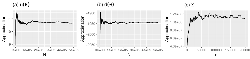
Figure 4: Results from the Ising model for the simulated lattice. (a) $\hat{u}_{N}(\theta)$ against the auxiliary sample size $N$, given a fixed value of $\theta$. (b) $\hat{d}_{N}(\theta)$ against the auxiliary sample size $N$, given the fixed value of $\theta$. (c) $\hat{\Sigma}_{n,N}$ against the posterior sample size $n$, given $N=$ 200,000.

Appendix E Choice of Tuning Parameters for Diagnostics

In this section, we show how we choose the auxiliary sample size $N$ and posterior sample size $n$ for our diagnostics in all examples of our manuscript.

E.1 The Ising Model

Figure 4 (a) shows how the approximation $\hat{u}_{N}(\theta)$ changes with an increasing size $N$ of auxiliary samples. The approximation appears to have stabilized around $N$ of 200,000. In Figure 4 (b), it is also observed that the approximation $\hat{d}_{N}(\theta)$ stabilizes around $N$ of 200,000. Thus we choose $N=$ 200,000 for ACD and AIKS. Figure 4 (c) shows the approximation $\hat{\Sigma}_{n,N}$ against the posterior sample size $n$. We observe that the approximation appears to have stabilized around $n$ of 120,000. Therefore, we choose $n=$ 120,000 for ACD.

E.2 A Social Network Model

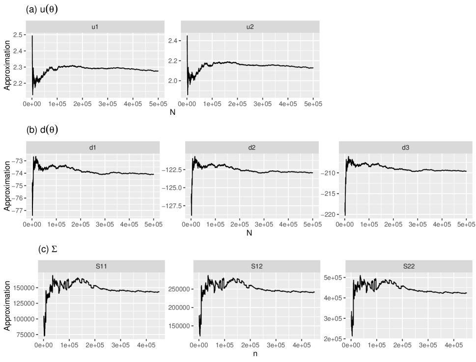
Figure 5: Results from ERGM for the simulated network. (a) $\hat{\boldsymbol{u}}_{N}(\boldsymbol{\theta})$ against the auxiliary sample size $N$, given a fixed value of $\boldsymbol{\theta}$. (b) $\hat{\boldsymbol{d}}_{N}(\boldsymbol{\theta})$ against the auxiliary sample size $N$, given the fixed value of $\theta$. (c) $\hat{\Sigma}_{n,N}$ against the posterior sample size $n$, given $N=$ 200,000.

Figure 5 (a) shows how the approximation $\hat{\boldsymbol{u}}_{N}(\boldsymbol{\theta})$ changes with an increasing size $N$ of auxiliary samples. The approximation appears to have stabilized around $N$ of 200,000. In Figure 5 (b), it is also observed that the approximation $\hat{\boldsymbol{d}}_{N}(\boldsymbol{\theta})$ stabilizes around $N$ of 200,000. Thus we choose $N=$ 200,000 for ACD and AIKS. Figure 5 (c) shows the approximation $\hat{\Sigma}_{n,N}$ against the posterior sample size $n$. We observe that the approximation appears to have stabilized around $n$ of 250,000. Therefore, we choose $n=$ 250,000 for ACD.

Figure 6: Results from the Conway–Maxwell–Poisson regression model for the takeover bids dataset. (a) $\hat{\boldsymbol{u}}_{N}(\boldsymbol{\theta})$ against the auxiliary sample size $N$, given a fixed value of $\boldsymbol{\theta}$. (b) $\hat{\boldsymbol{d}}_{N}(\boldsymbol{\theta})$ against the auxiliary sample size $N$, given the fixed value of $\boldsymbol{\theta}$. (c) $\hat{\Sigma}_{n,N}$ against the posterior sample size $n$, given $N=$ 200,000.

E.3 A Conway–Maxwell–Poisson Regression Model

Note that we only provide results regarding the first three elements of a vector or matrix because similar results are observed for the other elements. Figure 6 (a) shows how the approximation $\hat{\boldsymbol{u}}_{N}(\boldsymbol{\theta})$ changes with an increasing size $N$ of auxiliary samples. The approximation appears to have stabilized around $N$ of 200,000. In Figure 6 (b), it is also observed that the approximation $\hat{\boldsymbol{d}}_{N}(\boldsymbol{\theta})$ stabilizes around $N$ of 200,000. Thus we choose $N=$ 200,000 for ACD and AIKS. Figure 6 (c) shows the approximation $\hat{\Sigma}_{n,N}$ against the posterior sample size $n$, given $N=$ 200,000. We observe that the approximation appears to have stabilized around $n$ of 300,000. Therefore, we choose $n=$ 300,000 for ACD.

References

- Alquier et al., (2016) Alquier, P., Friel, N., Everitt, R., and Boland, A. (2016). Noisy Monte Carlo: Convergence of Markov chains with approximate transition kernels. Statistics and Computing, 26(1-2):29–47.
- Andrieu and Roberts, (2009) Andrieu, C. and Roberts, G. O. (2009). The pseudo-marginal approach for efficient Monte Carlo computations. Annals of Statistics, 37:697–725.
- Arcones and Gine, (1992) Arcones, M. A. and Gine, E. (1992). On the bootstrap of U and V statistics. The Annals of Statistics, 20:655–674.
- Atchadé et al., (2013) Atchadé, Y. F., Lartillot, N., and Robert, C. (2013). Bayesian computation for statistical models with intractable normalizing constants. Brazilian Journal of Probability and Statistics, 27(4):416–436.
- (5) Bartlett, M. S. (1953a). Approximate confidence intervals. Biometrika, 40(1/2):12–19.
- (6) Bartlett, M. S. (1953b). Approximate confidence intervals. II. More than one unknown parameter. Biometrika, 40(3/4):306–317.
- Beaumont, (2003) Beaumont, M. A. (2003). Estimation of population growth or decline in genetically monitored populations. Genetics, 164:1139–1160.
- Besag, (1974) Besag, J. (1974). Spatial interaction and the statistical analysis of lattice systems. Journal of the Royal Statistical Society: Series B, 36(2):192–225.
- Cameron and Johansson, (1997) Cameron, A. C. and Johansson, P. (1997). Count data regression using series expansions: With applications. Journal of Applied Econometrics, 12:203–223.
- Chanialidis et al., (2018) Chanialidis, C., Evers, L., Neocleous, T., and Nobile, A. (2018). Efficient Bayesian inference for COM-Poisson regression models. Statistics and Computing, 28:595–608.
- Chazottes et al., (2007) Chazottes, J. R., Collet, P., Külske, C., and Redig, F. (2007). Concentration inequalities for random fields via coupling. Probability Theory and Related Fields, 137:201–225.
- Chen and Seila, (1987) Chen, D. F. R. and Seila, A. F. (1987). Multivariate inference in stationary simulation using batch means. In Proceedings of the 19th conference on Winter Simulation, pages 302–304.
- Cheng et al., (2017) Cheng, J., Li, T., Levina, E., and Zhu, J. (2017). High-dimensional mixed graphical models. Journal of Computational and Graphical Statistics, 26:367–378.
- Conway and Maxwell, (1962) Conway, R. W. and Maxwell, W. L. (1962). Network dispatching by the shortest-operation discipline. Operations Research, 10:51–73.
- Cowles and Carlin, (1996) Cowles, M. K. and Carlin, B. P. (1996). Markov chain Monte Carlo convergence diagnostics: A comparative review. Journal of the American Statistical Association, 91(434):883–904.
- Damerdji, (1994) Damerdji, H. (1994). Strong consistency of the variance estimator in steady-state simulation output analysis. Mathematics of Operations Research, 19:494–512.
- Eddelbuettel and Francois, (2011) Eddelbuettel, D. and Francois, R. (2011). Rcpp: Seamless R and C++ integration. Journal of Statistical Software, 40:1–18.
- Fan et al., (2006) Fan, Y., Brooks, S. P., and Gelman, A. (2006). Output assessment for Monte Carlo simulations via the score statistic. Journal of Computational and Graphical Statistics, 15(1):178–206.
- Flegal et al., (2008) Flegal, J. M., Haran, M., and Jones, G. L. (2008). Markov chain monte carlo: Can we trust the third significant figure? Statistical Science, 23(2):250–260.
- Flegal and Jones, (2011) Flegal, J. M. and Jones, G. L. (2011). Implementing MCMC: Estimating with confidence. In Handbook of Markov Chain Monte Carlo, pages 175–197. Chapman and Hall/CRC.
- Fung et al., (2019) Fung, H.-T., Alwan, A., Wishart, J., and Huang, A. (2019). mpcmp: Mean-parametrized Conway–Maxwell–Poisson regression.
- Gelman and Rubin, (1992) Gelman, A. and Rubin, D. B. (1992). Inference from iterative simulation using multiple sequences. Statistical science, pages 457–472.
- Geweke et al., (1991) Geweke, J. F. et al. (1991). Evaluating the accuracy of sampling-based approaches to the calculation of posterior moments. Technical report, Federal Reserve Bank of Minneapolis.
- Geyer, (1992) Geyer, C. J. (1992). Practical markov chain monte carlo. Statistical science, pages 473–483.
- Goldstein et al., (2015) Goldstein, J., Haran, M., Simeonov, I., Fricks, J., and Chiaromonte, F. (2015). An attraction-repulsion point process model for respiratory syncytial virus infections. Biometrics, 71(2):376–385.
- Gorham and Mackey, (2015) Gorham, J. and Mackey, L. (2015). Measuring sample quality with Stein’s method. In Advances in Neural Information Processing Systems, volume 28.
- Gorham and Mackey, (2017) Gorham, J. and Mackey, L. (2017). Measuring sample quality with kernels. In Proceedings of the 34th International Conference on Machine Learning, pages 1292–1301.
- Guikema and Goffelt, (2008) Guikema, S. D. and Goffelt, J. P. (2008). A flexible count data regression model for risk analysis. Risk Analysis, 28:213–223.
- Hastings, (1970) Hastings, W. K. (1970). Monte Carlo sampling methods using Markov chains and their applications. Biometrika, 57(1):97–109.
- Huang, (2017) Huang, A. (2017). Mean-parametrized Conway–Maxwell–Poisson regression models for dispersed counts. Statistical Modelling, 17:359–380.
- Hughes et al., (2011) Hughes, J., Haran, M., and Caragea, P. C. (2011). Autologistic models for binary data on a lattice. Environmetrics, 22(7):857–871.
- Hunter, (2007) Hunter, D. R. (2007). Curved exponential family models for social networks. Social Networks, 29(2):216–230.
- Hunter and Handcock, (2006) Hunter, D. R. and Handcock, M. S. (2006). Inference in curved exponential family models for networks. Journal of Computational and Graphical Statistics, 15(3):565–583.
- Hunter et al., (2008) Hunter, D. R., Handcock, M. S., Butts, C. T., Goodreau, S. M., and Morris, M. (2008). ergm: A package to fit, simulate and diagnose exponential-family models for networks. Journal of Statistical Software, 24(3):1–29.
- Huskova and Janssen, (1993) Huskova, M. and Janssen, P. (1993). Consistency of the generalized bootstrap for degenerate U-statistics. The Annals of Statistics, 21:1811–1823.
- Ihaka and Gentleman, (1996) Ihaka, R. and Gentleman, R. (1996). R: A language for data analysis and graphics. Journal of Computational and Graphical Statistics, 5(3):299–314.
- Ising, (1925) Ising, E. (1925). Beitrag zur theorie des ferromagnetismus. Zeitschrift fürPhysik A Hadrons and Nuclei, 31(1):253–258.
- Jones et al., (2006) Jones, G. L., Haran, M., Caffo, B. S., and Neath, R. (2006). Fixed-width output analysis for Markov chain Monte Carlo. Journal of the American Statistical Association, 101:1537–1547.
- Kass et al., (1998) Kass, R. E., Carlin, B. P., Gelman, A., and Neal, R. M. (1998). Markov Chain Monte Carlo in Practice: A Roundtable Discussion. The American Statistician, 52(2):93–100.
- Lauritzen and Wermuth, (1989) Lauritzen, S. L. and Wermuth, N. (1989). Graphical models for associations between variables, some of which are qualitative and some quantitative. The Annals of Statistics, 17:31–57.
- Lee and Hastie, (2015) Lee, J. D. and Hastie, T. J. (2015). Learning the structure of mixed graphical models. Journal of Computational and Graphical Statistics, 24:230–253.
- Lee et al., (2019) Lee, J. E., Nicholls, G. K., and Ryder, R. J. (2019). Calibration Procedures for Approximate Bayesian Credible Sets. Bayesian Analysis, 14(4):1245–1269.
- Lenz, (1920) Lenz, W. (1920). Beitrag zum Verständnis der magnetischen Erscheinungen in festen Körpern. Physikalische Zeitschrift, 21:613–615.
- Liang, (2010) Liang, F. (2010). A double Metropolis-Hastings sampler for spatial models with intractable normalizing constants. Journal of Statistical Computation and Simulation, 80(9):1007–1022.
- Liang et al., (2016) Liang, F., Jin, I. H., Song, Q., and Liu, J. S. (2016). An adaptive exchange algorithm for sampling from distributions with intractable normalizing constants. Journal of the American Statistical Association, 111(513):377–393.
- Liu et al., (2016) Liu, Q., Lee, J. D., and Jordan, M. (2016). A kernelized Stein discrepancy for goodness-of-fit tests. In Proceedings of the 33rd International Conference on Machine Learning, pages 276–284.
- Lyne et al., (2015) Lyne, A. M., Girolami, M., Atchadé, Y., Strathmann, H., and Simpson, D. (2015). On Russian Roulette estimates for Bayesian inference with doubly-intractable likelihoods. Statistical Science, 30(4):443–467.
- Metropolis et al., (1953) Metropolis, N., Rosenbluth, A. W., Rosenbluth, M. N., Teller, A. H., and Teller, E. (1953). Equation of state calculations by fast computing machines. The journal of chemical physics, 21(6):1087–1092.
- Møller et al., (2006) Møller, J., Pettitt, A. N., Reeves, R., and Berthelsen, K. K. (2006). An efficient Markov chain Monte Carlo method for distributions with intractable normalising constants. Biometrika, 93(2):451–458.
- Müller, (1997) Müller, A. (1997). Integral probability metrics and their generating classes of functions. Advances in Applied Probability, 29(2):429–443.
- Murray et al., (2006) Murray, I., Ghahramani, Z., and Mackay, D. J. C. (2006). MCMC for doubly-intractable distributions. In Proceedings of the 22nd Annual Conference on Uncertainty in Artificial Intelligence, pages 359–366.
- Park and Haran, (2018) Park, J. and Haran, M. (2018). Bayesian inference in the presence of intractable normalizing functions. Journal of the American Statistical Association, 113(523):1372–1390.
- Park and Haran, (2020) Park, J. and Haran, M. (2020). A function emulation approach for doubly intractable distributions. Journal of Computational and Graphical Statistics, 29(1):66–77.
- Propp and Wilson, (1996) Propp, J. G. and Wilson, D. B. (1996). Exact sampling with coupled Markov chains and applications to statistical mechanics. Random Structures & Algorithms, 9(1-2):223–252.
- Rao et al., (2016) Rao, V., Lin, L., and Dunson, D. B. (2016). Data augmentation for models based on rejection sampling. Biometrika, 103:319–335.
- Ribeiro et al., (2020) Ribeiro, E. E., Zeviani, W. M., Bonat, W. H., Demetrio, C. G., and Hinde, J. (2020). Reparametrization of COM–Poisson regression models with applications in the analysis of experimental data. Statistical Modelling, 20:443–466.
- Robert and Casella, (2004) Robert, C. P. and Casella, G. (2004). Monte Carlo statistical methods. Springer.
- Robins et al., (2007) Robins, G., Pattison, P., Kalish, Y., and Lusher, D. (2007). An introduction to exponential random graph (p*) models for social networks. Social Networks, 29(2):173–191.
- Roy, (2020) Roy, V. (2020). Convergence diagnostics for Markov chain Monte Carlo. Annual Review of Statistics and Its Application, 7:387–412.
- Sáez-Castillo and Conde-Sánchez, (2013) Sáez-Castillo, A. J. and Conde-Sánchez, A. (2013). A hyper-Poisson regression model for overdispersed and underdispersed count data. Computational Statistics and Data Analysis, 61:148–157.
- Shmueli et al., (2005) Shmueli, G., Minka, T. P., Kadane, J. B., Borle, S., and Boatwright, P. (2005). A useful distribution for fitting discrete data: Revival of the Conway–Maxwell–Poisson distribution. Journal of the Royal Statistical Society: Series C, 54:127–142.
- Stein, (1972) Stein, C. (1972). A bound for the error in the normal approximation to the distribution of a sum of dependent random variables. In Proceedings of the Sixth Berkeley Symposium on Mathematical Statistics and Probability, volume 2, pages 583–602.
- Strauss, (1975) Strauss, D. J. (1975). A model for clustering. Biometrika, 62(2):467–475.
- Vats et al., (2019) Vats, D., Flegal, J. M., and Jones, G. L. (2019). Multivariate output analysis for Markov chain Monte Carlo. Biometrika, 106:321–337.
- Vats et al., (2022) Vats, D., Gonçalves, F., Łatuszyński, K., and Roberts, G. (2022). Efficient Bernoulli factory Markov chain Monte Carlo for intractable posteriors. Biometrika, 109:369–385.
- Xing et al., (2019) Xing, H., Nicholls, G. K., and Lee, J. E. (2019). Calibrated approximate Bayesian inference. In Proceedings of the 36th International Conference on Machine Learning, pages 6912–6920.