Low-rank statistical finite elements for scalable model-data synthesis

Abstract

Statistical learning additions to physically derived mathematical models are gaining traction in the literature. A recent approach has been to augment the underlying physics of the governing equations with data driven Bayesian statistical methodology. Coined statFEM, the method acknowledges a priori model misspecification, by embedding stochastic forcing within the governing equations. Upon receipt of additional data, the posterior distribution of the discretised finite element solution is updated using classical Bayesian filtering techniques. The resultant posterior jointly quantifies uncertainty associated with the ubiquitous problem of model misspecification and the data intended to represent the true process of interest. Despite this appeal, computational scalability is a challenge to statFEM’s application to high-dimensional problems typically experienced in physical and industrial contexts. This article overcomes this hurdle by embedding a low-rank approximation of the underlying dense covariance matrix, obtained from the leading order modes of the full-rank alternative. Demonstrated on a series of reaction-diffusion problems of increasing dimension, using experimental and simulated data, the method reconstructs the sparsely observed data-generating processes with minimal loss of information, in both the posterior mean and variance, paving the way for further integration of physical and probabilistic approaches to complex systems.

1 Introduction

The statistical finite element method (statFEM) [1] provides a novel statistical construction of the finite element method (FEM) to reconcile imperfect models with observational data. Potential model misspecification, as represented by a Gaussian process ($\mathcal{GP}$), is addressed through sequentially updating the FEM coefficients upon the arrival of observed data, within a filtering context, to compute a physics-informed posterior distribution. In [2], it is seen that for 1D nonlinear partial differential equations (PDEs), statFEM is able to give an accurate approximation to the underlying data generating process, with uncertainty quantification (UQ), synthesising physics and data to give an interpretable posterior distribution. Utilising such an approach allows for the application of simpler computational models, correcting for their possible deficiencies with data. This approach is also shown to be beneficial in small data regimes.

Recent advances in both the computational physics and machine learning communities have seen additional approaches proposed for combining physics and data. In [3], a sparse regression approach is taken, to learn the underlying PDE from spatio-temporal measurements inside the problem domain, building on the similar work of [4], to address system identification from a library of candidate functions. Neural networks can also be used, for both data-driven solution and system identification, and also for estimating optimal discretisations from data [5, 6]. Perhaps the most similar to statFEM is [7], where a $\mathcal{GP}$ prior is placed over the PDE variable, making the covariance kernel encode all a priori physical assumptions. This allows for system identification through transforming PDE coefficients into $\mathcal{GP}$ kernel hyperparameters, the estimation of which is well-studied [8].

StatFEM, instead, places a $\mathcal{GP}$ prior over the forcing of the PDE and focuses on updating solutions, combining methodology from Bayesian inversion [9] and data assimilation [10]. As in Bayesian inversion, statFEM uses a Gaussian prior placed over a function inside of the governing PDE. Though instead of estimating the posterior distribution of this unknown function, statFEM proceeds to sequentially update the discretised PDE solution, as in data assimilation. However the model is not treated as a black-box function, as we embed the uncertainty inside of the PDE formulation, and discretise the stochastic dynamics.

As presented, applying the statFEM methodology to high-dimensional systems is challenging. For the successful adoption of statFEM a scalable formulation for high-dimensional model-data synthesis is required, and this is the focus of this paper, for, in particular, nonlinear, time-dependent problems. We build on the extended Kalman filter (ExKF, [10]) method of [2], and study a scalable version of the statFEM methodology in the context of reaction-diffusion (RD) systems. To scale the method, we make a low-rank approximation to the posterior covariance matrix, and embed this within the ExKF; see [11, 12, 13, 14], for similar approaches.

Common examples of low-rank filters are the particle filter [15] and the ensemble Kalman filter (EnKF) [16]. However for high-dimensional systems the particle filter is known to suffer from particle collapse [17], and the ensemble Kalman filter, whilst accurate for the mean, can fail to provide accurate UQ [14]. Our interest in the low-rank ExKF (LR-ExKF) is motivated by additional results in [14], which show that a low-rank extended Kalman filter can provide accurate UQ for regularly observed nonlinear dissipative systems, similar to what is considered here.

We study the method in the context of RD systems as they are canonical examples of nonlinear, time-dependent phenomena in 2D, providing the necessary increase in state dimension from 1D examples considered previously. Systems often consist of coupled sets of equations, further increasing the dimensionality. They are an appropriate candidate for finite element methods, due to being parabolic [18], with potentially complex geometries, and are an appropriate test-case for filtering; the dynamics are not highly nonlinear, so the LR-ExKF can be applied without modification. However the methodology is not restricted to RD systems and can be applied to any nonlinear, time-dependent PDE for which finite element discretisations are appropriate. The method can also be applied to linear PDEs, where the algorithm gives the standard Kalman filter [19], and to static PDEs, in which the algorithm reduces to the iterative application of Bayes theorem.

The contribution of this paper is a scalable statFEM that can be applied to systems with a high state dimension. This is presented, with a self-contained introduction to statFEM, in Section 2, in the context of RD equations. We demonstrate the method in Section 3, on a series of examples. The first is a 1D example with experimental data, and we show that the LR-ExKF is able to accurately reproduce the full-rank ExKF, with relative errors of $\mathcal{O}(10^{-6})$ on the mean and $\mathcal{O}(10^{-5})$ on the variance. The next two examples deal with synthetic data, using the Oregonator [20, 21], a 2D system of two coupled PDEs, and we demonstrate scalability, taking the state dimension up to $132,098$ degrees-of-freedom (DOFs). Examples show that the LR-ExKF accurately reproduces the data generating process under misspecified initial conditions, with relative errors of order $\mathcal{O}(10^{-2})$ in the posterior mean. We also use the effective rank [22, 23] to verify the effective dimensionality of the covariance matrix, ensuring that the number of modes chosen is adequate. Section 4 concludes the paper, and the Appendix includes two additional examples of interest to practitioners, dealing with parameter estimation (C) and filter divergence (D). We also provide code to reproduce all results and figures in this paper, available at https://github.com/connor-duffin/low-rank-statfem.

2 Methodology: low-rank statFEM

We introduce the methodology using a general RD system, given by the semilinear parabolic PDE

$$\begin{gathered}\partial_{t}u=\kappa\nabla^{2}u+r(u)+\xi,\quad\text{ in }\Omega,\\ \nabla u\cdot\mathbf{n}=0,\quad\text{ on }\partial\Omega,\\ u(\mathbf{x},0)=u_{0},\quad u:=u(\mathbf{x},t)\in\mathbb{R},\\ \mathbf{x}\in\Omega\subset\mathbb{R}^{d},\quad t\in[0,T].\end{gathered}$$ (1)

Equation 1 describes the evolution of a system state (e.g. concentration of chemical species) which diffuses throughout the medium and has nonlinear interactions. All parameters of Equation (1) above are assumed known and are denoted by $\Lambda$. In this section, without loss of generality, we deal with single-state equations with $u\in\mathbb{R}$. Extensions to systems of equations with states $\bm{u}\in\mathbb{R}^{s}$ are covered in Section 3.

A $\mathcal{GP}$, $\xi:=\xi(\mathbf{x},t)$, is introduced inside of the PDE to represent prior uncertainty in the model specification:

$$\xi\sim\mathcal{GP}(0,\delta(t-t^{\prime})\cdot k_{\theta}(\mathbf{x},\mathbf{x}^{\prime})).$$ (2)

The spatial covariance kernel $k_{\theta}(\cdot,\cdot)$ encodes information on model error; we use the squared exponential kernel [8]

$$k_{\theta}(\mathbf{x},\mathbf{x}^{\prime})=\rho^{2}\exp\left(-\frac{\lVert\mathbf{x}-\mathbf{x}^{\prime}\rVert_{2}^{2}}{2\ell^{2}}\right)$$

under the a priori assumption that model errors are spatially smooth. Hyperparameters $\bm{\theta}=(\rho,\ell)$ respectively parameterise the variance and correlation length-scales of the model error, and are either set to fixed values a priori or estimated using maximum-a-posteriori methods [24]. Hyperparameter estimation is discussed after the algorithm presentation and is illustrated in C.

Delta correlations in time have the implication that $\xi$ is the weak derivative of a function-valued Wiener process such that $\xi(\mathbf{x},t+\Delta_{t})-\xi(\mathbf{x},t)\sim\mathcal{GP}(0,\Delta_{t}k_{\theta}(\mathbf{x},\mathbf{x}^{\prime}))$. We assume that $\xi(\mathbf{x},0)\equiv 0$, and thus $\xi(\mathbf{x},1)\sim\mathcal{GP}(0,k_{\theta}(\mathbf{x},\mathbf{x}^{\prime}))$. Spatially, the process inherits the regularity as implied by $k_{\theta}(\cdot,\cdot)$, which in this work is assumed to give $\xi(\mathbf{x},\cdot)\in L^{2}(\Omega)$. For further details we refer to [25].

Spatial discretisation proceeds through multiplying by testing functions $\varphi\in H^{1}(\Omega)$ and integrating over the problem domain. This gives the semidiscrete weak form

$$\langle\partial_{t}u,\varphi\rangle+\kappa\mathcal{A}(u,\varphi)=\langle r(u),\varphi\rangle+\langle\xi,\varphi\rangle,\quad\forall\varphi\in H^{1}(\Omega),$$

where $\mathcal{A}(u,\varphi)=\int_{\Omega}\nabla u\cdot\nabla\varphi\,\mathrm{d}\mathbf{x}$, $\langle f,g\rangle=\int_{\Omega}f\,g\,\mathrm{d}\mathbf{x}$: these are respectively the bilinear form induced by the Laplacian operator and the $L^{2}(\Omega)$ inner product. Neumann boundary conditions result in the boundary terms dropping out of the weak form.

The finite element mesh is given by subdividing the domain $\Omega$ into the triangulation $\Omega_{h}\subseteq\Omega$ with vertices $\{\mathbf{x}_{j}\}_{j=1}^{n_{u}}$, where the maximal length of the sides of the triangulation is given by $h$. The polynomial basis functions $\{\phi_{j}\}_{j=1}^{n_{u}}$ are defined on the mesh, having the property that $\phi_{j}(\mathbf{x}_{i})=\delta_{ij}$. Letting $V_{h}=\mathrm{span}\{\phi_{i}\}_{i=1}^{n_{u}}$, so that $V_{h}\subset H^{1}(\Omega)$, we write the approximation $u_{h}(\mathbf{x},t)=\sum_{i=1}^{n_{u}}u_{i}(t)\phi_{i}(\mathbf{x})$. In the finite dimensional space $V_{h}$ the weak form is

$$\langle\partial_{t}u_{h},\phi_{j}\rangle+\kappa\mathcal{A}(u_{h},\phi_{j})=\langle r(u_{h}),\phi_{j}\rangle+\langle\xi,\phi_{j}\rangle,\quad j=1,\ldots,n_{u},$$

which corresponds to the $n_{u}$-dimensional SDE for the FEM coefficients

$$\mathbf{M}\,\mathrm{d}\mathbf{u}+\kappa\mathbf{A}\mathbf{u}\,\mathrm{d}t=\tilde{\mathbf{r}}(\mathbf{u})\,\mathrm{d}t+\mathrm{d}\bm{\beta},$$

where $\mathbf{M}_{ji}=\langle\phi_{i},\phi_{j}\rangle$, $\mathbf{A}_{ji}=\mathcal{A}(\phi_{i},\phi_{j})$, $\tilde{\mathbf{r}}(\mathbf{u})_{j}=\langle r(u_{h}),\phi_{j}\rangle$, and $\mathbf{u}(t)=(u_{1}(t),\ldots,u_{n_{u}}(t))^{\top}$. The additive noise process $\bm{\beta}(t):=(\beta_{1}(t),\ldots\beta_{n_{u}}(t))^{\top}$ has the increments

$$\bm{\beta}(t+\Delta_{t})-\bm{\beta}(t)\sim\mathcal{N}(\mathbf{0},\Delta_{t}\mathbf{G}_{\theta}),\quad\mathbf{G}_{\theta,{ij}}=\langle\phi_{i},\langle k_{\theta}(\cdot,\cdot),\phi_{j}\rangle\rangle.$$

In the absence of additive noise (i.e., for the ODE case), under bounded derivative conditions on $r$, solutions will be unique, by the Picard-Lindelöf theorem [18]. We use Crank-Nicolson for time integration; writing $\mathbf{u}_{n}=(u_{1}(n\Delta_{t}),\ldots,u_{n_{u}}(n\Delta_{t}))^{\top}$, for timestep size $\Delta_{t}>0$, yields a fully discrete system accurate to order $\mathcal{O}(h^{2}+\Delta_{t}^{2})$

$$\mathbf{M}\left(\mathbf{u}_{n}-\mathbf{u}_{n-1}\right)+\Delta_{t}\kappa\mathbf{A}\mathbf{u}_{n-1/2}=\Delta_{t}\tilde{\mathbf{r}}(\mathbf{u}_{n-1/2})+\mathbf{e}_{n-1},\quad\mathbf{e}_{n-1}\sim\mathcal{N}(\mathbf{0},\Delta_{t}\mathbf{G}_{\theta}),$$ (3)

in which $\mathbf{u}_{n-1/2}=(\mathbf{u}_{n}+\mathbf{u}_{n-1})/2$. In practice any appropriate time discretisation can be implemented and the choice will be problem-dependent. In this paper Crank-Nicolson discretisations ensure stability, motivated by the example given in D. In this example, it is seen that for sufficiently nonlinear dynamics the resultant filtering algorithm may diverge when the time discretisation is of implicit-explicit-type [26]. The divergence is avoided when Crank-Nicolson is used.

Given a fixed set of hyperparameters $\bm{\theta}$, the Euler-Maruyama discretisation [27] of Equation (3) draws sample paths from the measure $p(\mathbf{u}_{n}\>|\>\bm{\theta},\Lambda)$ for each $n=1,\ldots,n_{t}$. These samples are drawn from a physics-motivated prior distribution, which can be updated, via Bayes theorem, to give a posterior distribution over the FEM coefficients. Model misspecification can then be directly corrected for through computing the posterior distribution.

The data generating process is assumed to be $\mathbf{y}_{n}=\mathbf{H}\mathbf{u}_{n}+\bm{\eta}_{n}$. The data $\mathbf{y}_{n}\in\mathbb{R}^{n_{y}}$ are assumed to be corrupted by an independent measurement noise process, $\bm{\eta}_{n}\sim\mathcal{N}(0,\sigma^{2}\mathbf{I}_{n_{y}})$, and are observed via the linear observation operator $\mathbf{H}:\mathbb{R}^{n_{u}}\to\mathbb{R}^{n_{y}}$. For each $n$, this defines the likelihood $p(\mathbf{y}_{n}\>|\>\mathbf{u}_{n},\sigma)=\mathcal{N}(\mathbf{H}\mathbf{u}_{n},\sigma^{2}\mathbf{I}_{n_{y}})$. The posterior distribution $p(\mathbf{u}_{n}\>|\>\mathbf{y}_{1:n},\bm{\theta},\sigma,\Lambda)$, with $\mathbf{y}_{1:n}=(\mathbf{y}_{1},\ldots,\mathbf{y}_{n})$, can be computed through nonlinear filtering algorithms. In previous work the ExKF and EnKF were used [2], however as discussed in the introduction these algorithms can perform poorly in high-dimensional settings. To circumvent this computational bottleneck we use the LR-ExKF algorithm, which computes the Gaussian approximation $p(\mathbf{u}_{n}\>|\>\mathbf{y}_{1:n},\bm{\theta},\sigma,\Lambda)\approx\mathcal{N}(\mathbf{m}_{n},\mathbf{C}_{n})$ from a low-rank approximation of the state covariance matrix $\mathbf{C}_{n}=\mathbf{L}_{n}\mathbf{L}_{n}^{\top}$. This is constructed with the leading eigenvalues and eigenvectors of the prior covariance matrix $\mathbf{G}_{\theta}$ and the previous timestep covariance $\mathbf{C}_{n-1}$. For similar approaches see [11, 12, 13, 14].

Assume that the distribution of the previous state is given by $p(\mathbf{u}_{n-1}\>|\>\mathbf{y}_{1:n-1},\bm{\theta},\sigma,\Lambda)=\mathcal{N}(\mathbf{m}_{n-1},\mathbf{C}_{n-1})$, with $\mathbf{C}_{n-1}=\mathbf{L}_{n-1}\mathbf{L}_{n-1}^{\top}$, $\mathbf{L}_{n-1}\in\mathbb{R}^{n_{u}\times k}$. Furthermore, assume that a low-rank square root of $\mathbf{G}_{\theta}=\mathbf{G}_{\theta}^{1/2}\mathbf{G}_{\theta}^{\top/2}$ is also available, where $\mathbf{G}_{\theta}^{1/2}\in\mathbb{R}^{n_{u}\times k^{\prime}}$. Also note that $D_{n}\tilde{\mathbf{r}}:=\partial\tilde{\mathbf{r}}(\mathbf{u}_{n-1/2})/\partial\mathbf{u}_{n}$, the Jacobian matrix.

For all timesteps $n=1,\ldots,n_{t}$, the LR-ExKF proceeds as:

1. (Prediction step) Solve

   $$\mathbf{M}\left(\hat{\mathbf{m}}_{n}-\mathbf{m}_{n-1}\right)+\Delta_{t}\kappa\mathbf{A}\hat{\mathbf{m}}_{n-1/2}=\Delta_{t}\tilde{\mathbf{r}}(\hat{\mathbf{m}}_{n-1/2}),$$

   for the prediction mean $\hat{\mathbf{m}}_{n}$ and compute the prediction covariance square root:

   $$\tilde{\mathbf{L}}_{n}=\Big{[}\left(\mathbf{M}+\Delta_{t}(\kappa\mathbf{A}+D_{n}\tilde{\mathbf{r}})\right)^{-1}\left(\mathbf{M}+\Delta_{t}D_{n-1}\tilde{\mathbf{r}}\right)\mathbf{L}_{n-1},$$

   $$\Delta_{t}\left(\mathbf{M}+\Delta_{t}\kappa\mathbf{A}+\Delta_{t}D_{n}\tilde{\mathbf{r}}\right)^{-1}\mathbf{G}_{\theta}^{1/2}\Big{]}$$

   noting that $\tilde{\mathbf{L}}_{n}\tilde{\mathbf{L}}_{n}^{\top}=\hat{\mathbf{C}}_{n}$ (the prediction covariance), and that $\tilde{\mathbf{L}}_{n}\in\mathbb{R}^{n_{u}\times(k+k^{\prime})}$. Each column of $\tilde{\mathbf{L}}_{n}$ can be formed in parallel; see the following discussion for further details.

2. (Truncation step) Take the eigendecomposition $\tilde{\mathbf{L}}_{n}^{\top}\tilde{\mathbf{L}}_{n}=\mathbf{V}_{n}\bm{\Sigma}_{n}\mathbf{V}_{n}^{\top}$, where $\bm{\Sigma}_{n}=\mathrm{diag}(\varsigma_{1},\ldots,\varsigma_{k+k^{\prime}})$. Approximate $\hat{\mathbf{L}}_{n}=\tilde{\mathbf{L}}_{n}\left[\mathbf{V}_{n}\right]_{:,1:k}$ for the highest magnitude $k$ modes, so the prediction covariance is $\hat{\mathbf{C}}_{n}=\hat{\mathbf{L}}_{n}\hat{\mathbf{L}}_{n}^{\top}$.

3. (Update step) Update the mean:

   $$\mathbf{m}_{n}=\hat{\mathbf{m}}_{n}+(\mathbf{H}\hat{\mathbf{C}}_{n})^{\top}\left(\mathbf{H}\hat{\mathbf{C}}_{n}\mathbf{H}^{\top}+\sigma^{2}\mathbf{I}_{n_{y}}\right)^{-1}(\mathbf{y}_{n}-\mathbf{H}\hat{\mathbf{m}}_{n}).$$

   And the covariance:

   $$\mathbf{L}_{n}=\hat{\mathbf{L}}_{n}\mathbf{R}_{n},$$

   $$\mathbf{R}_{n}\mathbf{R}_{n}^{\top}=\mathbf{I}_{k}-\hat{\mathbf{L}}_{n}^{\top}\mathbf{H}^{\top}(\mathbf{H}\hat{\mathbf{C}}_{n}\mathbf{H}^{\top}+\sigma^{2}\mathbf{I}_{n_{y}})^{-1}\mathbf{H}\hat{\mathbf{L}}_{n},$$

   using a Cholesky decomposition or otherwise.

If $k=k^{\prime}=n_{u}$ then the LR-ExKF recovers the full ExKF exactly. If the datum $\mathbf{y}_{n}$ is missing then only the prediction and truncation steps are completed, to produce the posterior $p(\mathbf{u}_{n}\>|\>\mathbf{y}_{1:n},\bm{\theta},\sigma,\Lambda)\equiv p(\mathbf{u}_{n}\>|\>\mathbf{y}_{1:n-1},\bm{\theta},\sigma,\Lambda)$.

Discussion

First we compare the ExKF and LR-ExKF in terms of memory and operation counts. For a general reference to these matrix computations we refer to [28]. The standard ExKF requires that $\mathbf{C}_{n}$ and $\mathbf{G}_{\theta}$ are stored in memory, which is $\mathcal{O}(n_{u}^{2})$ in space. For large DOF problems this is infeasible, and provides the main motivation for the low-rank approach. If one employs the standard ExKF, though, then the prediction step for the covariance matrix requires the solution of the sparse $n_{u}\times n_{u}$ matrix $\mathbf{M}+\Delta_{t}(\kappa\mathbf{A}+D_{n}\tilde{\mathbf{r}})$, $2n_{u}$ times for each timestep. For large $n_{u}$ this becomes prohibitively expensive. If using a direct solver is feasible, then this can be slightly mitigated by computing the LU factorisation of $\mathbf{M}+\Delta_{t}(\kappa\mathbf{A}+D_{n}\tilde{\mathbf{r}})$, and reusing the factors when solving for each column of $\tilde{\mathbf{L}}_{n-1}$, though this still requires running forward- and back-substitution $2n_{u}$ times per timestep.

Furthermore, the update step requires the solution of the system $\mathbf{H}\hat{\mathbf{C}}_{n}\mathbf{H}^{\top}+\sigma^{2}\mathbf{I}_{n_{y}}$, $n_{u}$ times, for each timestep, which requires $\mathcal{O}(n_{y}^{3}/3)$ operations to take the Cholesky decomposition and $\mathcal{O}(n_{y}^{2}n_{u})$ to solve.

In comparison, LR-ExKF requires solving $\mathbf{M}+\Delta_{t}(\kappa\mathbf{A}+D_{n}\tilde{\mathbf{r}})$, $k+k^{\prime}$ times for each timestep, and is $\mathcal{O}((k+k^{\prime})n_{u})$ in space. The truncation step incurs a cost of $\mathcal{O}((k+k^{\prime})^{3})$ to compute the eigendecomposition. The update step has a cost of $\mathcal{O}(n_{y}^{3}/3)$ operations to take the Cholesky factorisation of $\mathbf{H}\hat{\mathbf{C}}_{n}\mathbf{H}^{\top}+\sigma^{2}\mathbf{I}_{n_{y}}$, but requires only $k$ solves, to give the cost $\mathcal{O}(n_{y}^{2}k)$. Finally, the cost of the Cholesky factor $\mathbf{R}_{n}$ is $\mathcal{O}(k^{3}/3)$. However, note that $k\ll n_{u}$, and in our experience the cost of these decompositions is dwarfed by solving the system in the prediction step.

Note also that each column of the prediction covariance square root $\tilde{\mathbf{L}}_{n}$ is able to be computed in parallel. As each column requires solving $\mathbf{M}+\Delta_{t}(\kappa\mathbf{A}+D_{n}\tilde{\mathbf{r}})$ this can result in lower runtimes, especially when combined with, for example, algebraic multigrid solvers [29]. This parallelisation is likely to be necessary when scaling up the LR-ExKF to larger systems than those considered here, such as high-dimensional 3D models. This is also similar to the parallelisation potential of the EnKF prediction step, which has enabled widespread adoption of this algorithm [30].

It is also assumed that the covariance spectrum of $\mathbf{G}_{\theta}$ is rapidly decaying so that the majority of the variance can be explained by $k^{\prime}\ll n_{u}$ dominant modes. In this work we use the squared-exponential covariance function, which is known to have a rapid spectral decay [31, 32]. For efficient methods to decompose $\mathcal{GP}$ covariance matrices into their leading eigenvalues we refer to [33, 34, 35, 36]. As the filter is initialised with the $l^{2}$-optimal low-rank square-root and the truncation step preserves the dominant modes of variation, it is thought that this scheme is able to provide accurate UQ; we plan to verify this in future work.

The low-rank approximation of the covariance matrix will lead to underestimation. If we write the prediction covariance as $\hat{\mathbf{C}}_{n}+\hat{\mathbf{C}}_{n,\mathrm{err}}$ then the norm of the discarded component is given by $\|\hat{\mathbf{C}}_{n,\mathrm{err}}\|=\varsigma_{k+1}$. This is noted in [12], where it is also commented that this underestimation could lead to similar problems as encountered in ensemble Kalman filtering, such as catastrophic filter divergence [22]. We have observed this when using unstable time-integration schemes, in the spiral wave regime; we refer to the D for full details. There is additional symmetry to the EnKF: both algorithms propagate a low-rank approximation to the covariance square root ($\mathbf{L}_{n}$ in the LR-ExKF; the ensemble in the EnKF), and make the Gaussian assumption in the update step. It is thought that the LR-ExKF is similar to an EnKF where the ensemble members are chosen to optimally represent the variance (in the $l^{2}$ sense), and the propagation is done through the tangent linear model.

To avoid inverting $\mathbf{H}\hat{\mathbf{C}}_{n}\mathbf{H}^{\top}+\sigma^{2}\mathbf{I}_{n_{y}}$, when $n_{y}\gg k$, the Woodbury matrix identity [13, 37] can be used

$$\left(\mathbf{H}\hat{\mathbf{C}}_{n}\mathbf{H}^{\top}+\sigma^{2}\mathbf{I}_{n_{y}}\right)^{-1} =\left(\mathbf{H}\hat{\mathbf{L}}_{n}(\mathbf{H}\hat{\mathbf{L}}_{n})^{\top}+\sigma^{2}\mathbf{I}_{n_{y}}\right)^{-1}$$

$$=\frac{1}{\sigma^{2}}\left(\mathbf{I}_{n_{y}}+\mathbf{H}\hat{\mathbf{L}}_{n}\left(\sigma^{2}\mathbf{I}_{k}+(\mathbf{H}\hat{\mathbf{L}}_{n})^{\top}(\mathbf{H}\hat{\mathbf{L}}_{n})\right)^{-1}(\mathbf{H}\hat{\mathbf{L}}_{n})^{\top}\right).$$

The dense $k\times k$ symmetric positive definite matrix $\sigma^{2}\mathbf{I}_{k}+(\mathbf{H}\hat{\mathbf{L}}_{n})^{\top}(\mathbf{H}\hat{\mathbf{L}}_{n})$ can be solved using the Cholesky decomposition [28].

$\mathcal{GP}$ hyperparameters $\bm{\theta}$ and noise standard deviation $\sigma$ can be estimated through maximum-a-posteriori (MAP) estimation [24]. To estimate parameters we assume the time evolving structure $\bm{\theta}:=\bm{\theta}_{n}$, $\sigma:=\sigma_{n}$ for all $n$, and that $\bm{\theta}_{n}$ and $\sigma_{n}$ are independent across time. Note that $\tilde{\mathbf{L}}_{n}\equiv\tilde{\mathbf{L}}_{n}(\bm{\theta}_{n})$, and writing $\bm{\theta}_{1:n}=(\bm{\theta}_{1},\ldots,\bm{\theta}_{n})$ and $\sigma_{1:n}=(\sigma_{1},\ldots,\sigma_{n})$, then the marginal likelihood is

$$p(\mathbf{y}_{n}\>|\>\mathbf{y}_{1:n-1},\bm{\theta}_{1:n},\sigma_{1:n},\Lambda)\sim\mathcal{N}\left(\mathbf{H}\hat{\mathbf{m}}_{n},\,\mathbf{H}\tilde{\mathbf{L}}_{n}(\bm{\theta}_{n})\big{(}\mathbf{H}\tilde{\mathbf{L}}_{n}(\bm{\theta}_{n})\big{)}^{\top}+\sigma_{n}^{2}\mathbf{I}_{n_{y}}\right).$$

The optimisation problem for the log-marginal-posterior is thus

$$\hat{\bm{\theta}}_{n},\hat{\sigma}_{n}=\operatorname*{arg\,max}_{\left(\bm{\theta}_{n},\sigma_{n}\right)}\left\{\log p(\mathbf{y}_{n}\>|\>\mathbf{y}_{1:n-1},\bm{\theta}_{1:n},\sigma_{1:n},\Lambda)+\log p(\bm{\theta}_{n})+\log p(\sigma_{n})\right\}.$$

In C, we use the weakly informative priors $\rho_{n}\sim\mathcal{N}_{+}(1,1^{2})$ and $\sigma_{n}\sim\mathcal{N}_{+}(0,1^{2})$, reflecting the a priori uncertainty in the optimal choices of these hyperparameters. For the optimisation routine, L-BFGS-B [38] with positivity constraints, as implemented in SciPy [39], has worked well in our experience.

3 Case studies

The methodology is demonstrated on three RD examples. The first is a verification of the method on a 1D example of cell RD, using the experimental data of [40], and shows a coherent synthesis of data with a prior physical model. It also confirms that the low-rank filter accurately reproduces the full-rank filter, with relative errors of $\mathcal{O}(10^{-6})$ for the mean, and $\mathcal{O}(10^{-4})$ for the variance.

The next two examples are in 2D, using the Oregonator RD model [20, 21], with misspecificied initial conditions. The first 2D example demonstrates that observations of a single component of the system can correct for misspecification on the unobserved component. The second 2D example studies the affect of increasing the mismatch variance $\rho$ on filter performance and also shows scalability, using a state dimension of $n_{u}=132,098$. Conditioning on data corrects for misspecification, and in both cases statFEM recovers the underlying data generating process to relative errors of $\mathcal{O}(10^{-2})$. In these examples, running the full-rank filter is prohibitively expensive, so we also use the effective rank of $\hat{\mathbf{L}}_{n}$ as a measure for filter performance.

The supplement contains two additional studies, which discuss the parameter estimation methodology, and a case of catastrophic filter divergence, respectively. Code to run all examples is available on a public GitHub repository , with all finite element discretisations done in Fenics [41].

3.1 Experimental data: verification

We consider a system of two coupled nonlinear RD equations, which model the densities of two different cell populations, as cells react with one another and diffuse throughout the domain, as discussed in [40]. The model is a coupled system of two nonlinear RD equations, with stochastic forcing. The combined system state is given by $\bm{w}=(u,v)\in\mathbb{R}^{2}$:

$$\begin{cases}u_{t}=Du_{xx}-k_{u}u+2k_{v}v(1-u-v)+\xi_{u},\\ v_{t}=Dv_{xx}+k_{u}u-k_{v}v(1-u-v)+\xi_{v},\\ u_{x}(0,t)=0,\quad u_{x}(1300,t)=0,\\ u:=u(x,t),\quad x\in[0,1300]\,\mu m,\quad t\in[0,60]\,h.\\ \end{cases}$$ (4)

Coefficients are set to $D=700\mu m^{2}/h$, $k_{u}=0.025$, $k_{v}=0.0725$, with initial conditions

$$\begin{cases}u(x,0)=v(x,0)=0,&x\in[400,900],\\ u(x,0)=v(x,0)=0.055,&\text{otherwise}.\end{cases}$$

In contrast to [40], who linearly interpolate the data to give their initial conditions, we assume the fixed piecewise initial conditions as above. Instead of interpolating the data at time $t=0$, we condition on it. Equation (4) is discretised using the standard linear polynomial “hat” basis functions, for each component, on a regular mesh with $200$ cells on the interval $[0,1300]$. Crank-Nicolson is used for the time discretisation, with timestep size $\Delta_{t}=0.1$.

Hyperparameters of $\xi_{u}$ and $\xi_{v}$ are set to the same values, which are constant across all times; this is to avoid propagating poor estimates through the simulation. The covariance structure of Equation (2), is used, and cross-correlations are assumed to be zero: $\mathbb{E}(\xi_{u}\xi_{v})\equiv 0$. Hyperparameters are set to $\rho=2\times 10^{-3}$ and $\ell=100$.

Laboratory data of this system is contained in the supplementary information of [40], freely available online. These data consist of observations of the two species at $4$ times, $t_{\text{obs}}=0,16,32,48$ hours. The concatenated state, $\mathbf{w}_{n}={(\mathbf{u}_{n}^{\top},\mathbf{v}_{n}^{\top})}^{\top}$, gives the data generating process $\mathbf{y}_{n}=\mathbf{H}\mathbf{w}_{n}+\bm{\eta}_{n}$ at the observation times, with noise $\bm{\eta}_{n}\sim\mathcal{N}(0,\sigma^{2}\mathbf{I}_{n_{y}})$, $\sigma=0.01$.

The posterior $p(\mathbf{w}_{n}\>|\>\mathbf{y}_{1:n},\bm{\theta},\sigma,\Lambda)=\mathcal{N}(\mathbf{m}_{n},\mathbf{L}_{n}\mathbf{L}_{n}^{\top})$ is computed with the LR-ExKF, using $k=k^{\prime}=32$ modes for both the state covariance, and for the covariances of the $\mathcal{GP}$s, $\xi_{u}$ and $\xi_{v}$. More than $99\%$ of the variance is retained in the variance truncation at each timestep. The resulting posterior means $\mathbf{m}_{n}^{u},\mathbf{m}_{n}^{v}$, and $95\%$ posterior credible intervals are shown for both the observation times and five hours after the observation times, in Figure 1. For the $v$ component, there is little discrepancy between the data and the prior assumed model, however for the $u$ component there is some degree of model mismatch, which conditioning on data can partially account for. The posterior means for each component across the entire space-time grid are also plotted in Figure 2, and demonstrate the immediate effects of conditioning on data at the times at which these data are observed.

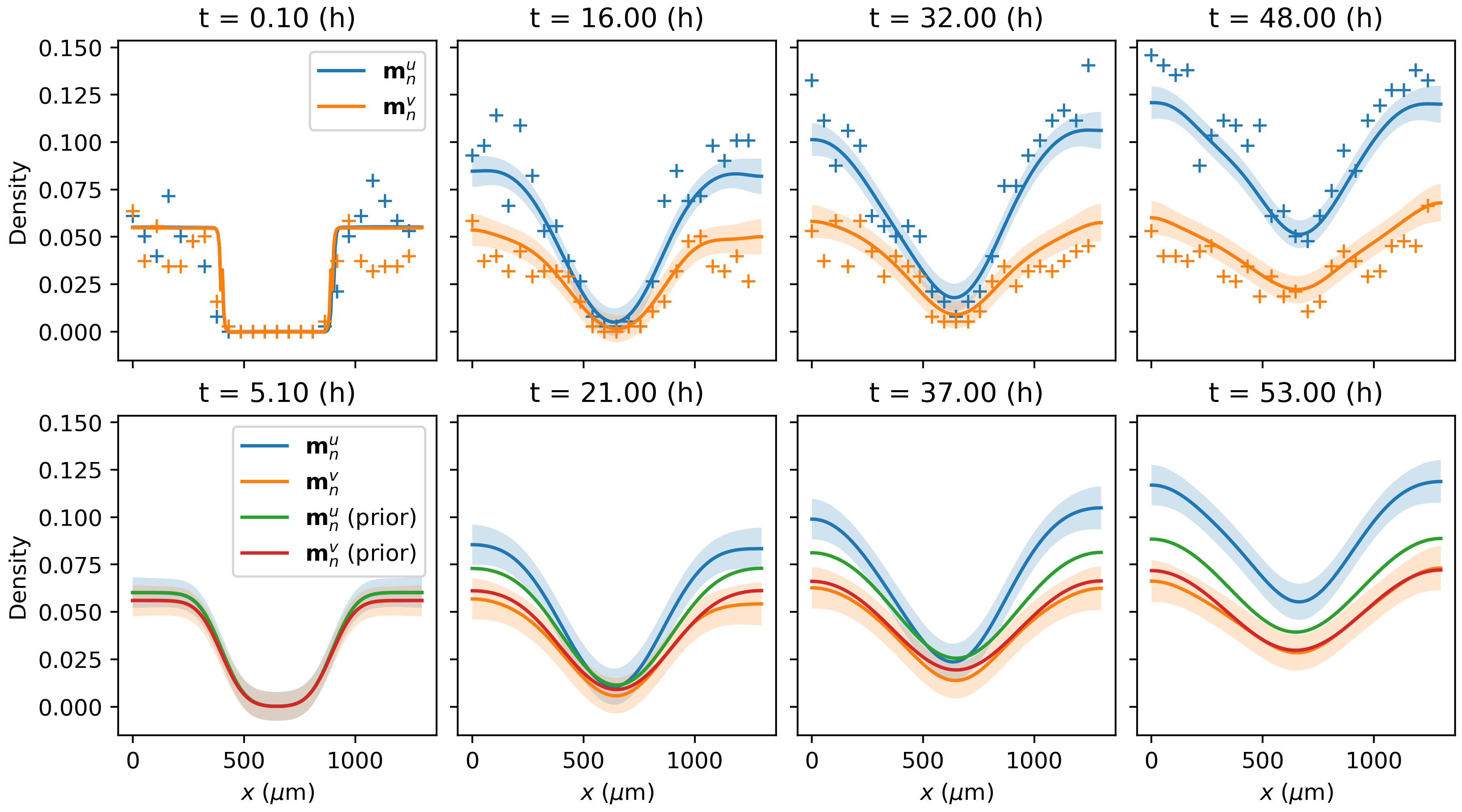
Figure 1: Observed data, posterior means, and 95% posterior credible intervals for the four observed data times (top), and posterior means and 95% posterior credible intervals for five hours after the observation times (bottom).

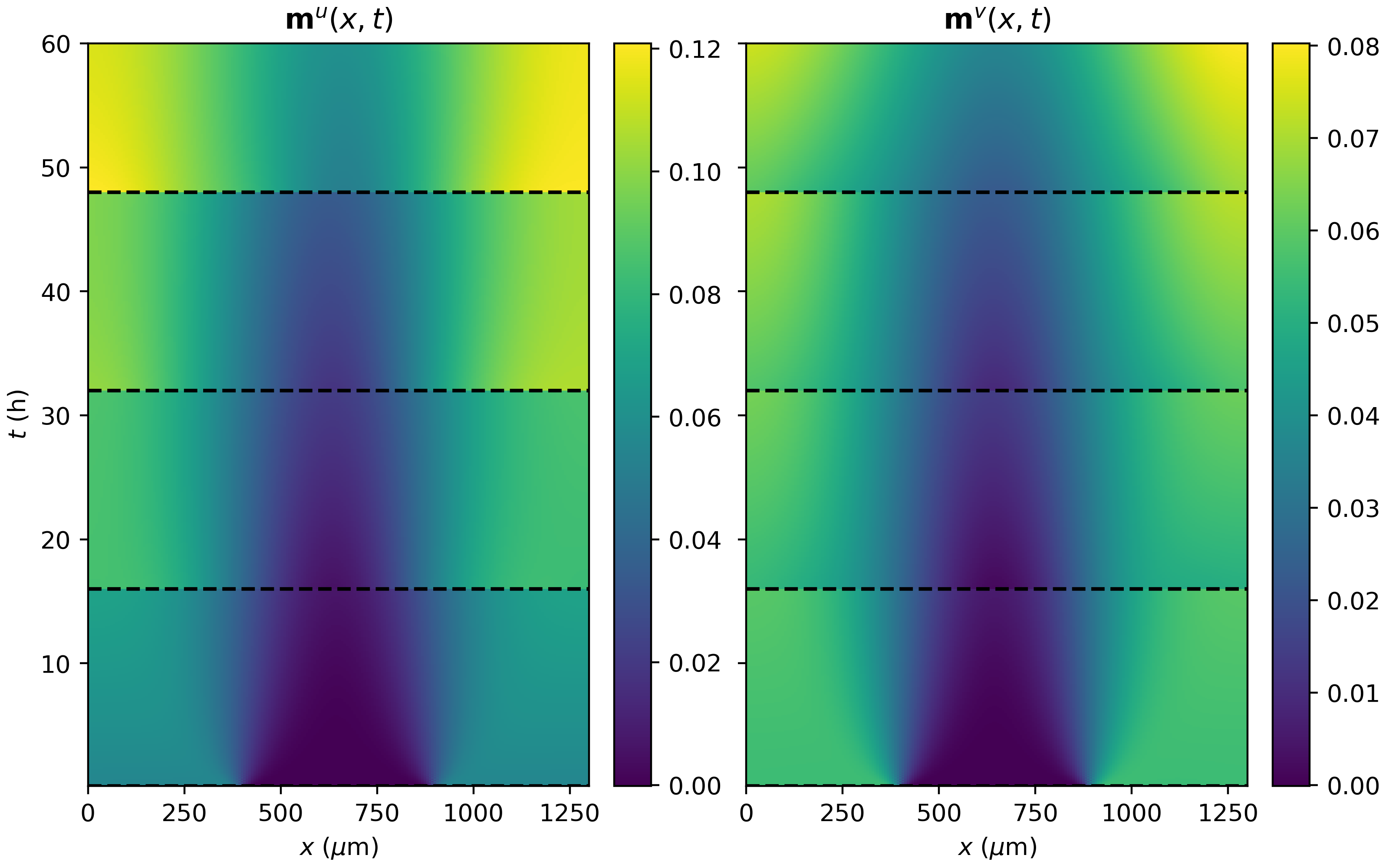
Figure 2: Space-time plot of the posterior means for each component. Times at which data are observed are shown with a dashed black line. On the $u$ component there is an immediate correction from data conditioning, not present in the $v$ component: the prior model for $v$ is more accurate.

The low- and full-rank ExKF’s are now compared through the posterior means and variances, in terms of the relative error

$$\frac{\lVert\mathbf{m}_{n}^{u}-\mathbf{m}_{n,LR}^{u}\rVert}{\lVert\mathbf{m}_{n}^{u}\rVert},\quad\frac{\lVert\mathrm{var}(\mathbf{u}_{n})-\mathrm{var}(\mathbf{u}_{n,LR})\rVert}{\lVert\mathrm{var}(\mathbf{u}_{n})\rVert},$$

with the norm $\lVert\cdot\rVert$ taken as the standard Euclidean norm (the $l^{2}$-norm).

Shown in Figure 3, for a fixed number of modes ($k=k^{\prime}=32$), the relative errors are small, at approximately $10^{-7}$ for the posterior mean, and $10^{-5}$ for the posterior variance. Sharp increases are observed at the times at which data is observed, in both the posterior mean and the posterior variance. The relative error at the end time of the simulation is also shown in Figure 4, as both $k$ and $k^{\prime}$ are increased. In either case, the errors are computed over $\{4,8,16,32,48,64\}$ modes, with either $k$ or $k^{\prime}$ fixed to $32$. In each case, as the variable number of modes increases the error decreases, with minor gains in the final error observed when going from $32$ to $64$ modes.

As $k$ is increased (Figure 4(a)), past $k=k^{\prime}=32$ there is a small increase in the accuracy of the filter, with a minor increase from $k=32$ to $k=48$. This minor increase is thought to be due to the inclusion of information available from the data, not present in the prior alone. As $k^{\prime}$ is increased (Figure 4(b)), past $k^{\prime}=k=32$ there is visually no gain from adding in additional modes in the prior, as these end up being truncated to $k=32$. In both cases, increasing from $48$ to $64$ modes shows little decrease in the posterior mean and variance errors. These results suggest that there is a number of effective modes that capture the dominant modes of variation; beyond some effective number of dimensions, taking more modes does not yield significant gains in accuracy.

The low-rank approximation of the prior covariance matrix has a large affect on the accuracy of the estimated posterior covariance matrix. Recall that in the problem specification the uncertainty is induced via the additive $\mathcal{GP}$, $\xi$, and no other sources of uncertainty are considered; if the covariance of $\xi$ is approximated to a sufficient degree then the low-rank approximation of the filter is accurate.

This can be seen from the ExKF approximation of the prior measure, which for exposition is considered in the case in which $\mathbf{G}_{\theta}$ is rank-deficient but is stored fully in memory. This gives an iterative approximation for the covariance matrix [2, Supplementary Information]

$$\hat{\mathbf{C}}_{n}=\mathbf{J}_{n}^{-1}(\mathbf{J}_{n-1}\mathbf{C}_{n-1}\mathbf{J}_{n-1}^{\top}+\mathbf{G}_{\theta})\mathbf{J}_{n}^{-\top},$$

where $\mathbf{J}_{n}$ is the Jacobian matrix of the FEM model with respect to $\mathbf{u}_{n}$, evaluated at $(\hat{\mathbf{m}}_{n},\mathbf{m}_{n-1})$. Given the recursive nature of computation and the fact that $\mathbf{C}_{0}=\mathbf{0}$ (due to the assumed initial conditions being exact) the prior covariance is a sum of matrix products with $\mathbf{G}_{\theta}$ and the Jacobian matrices, at each timestep. The prior covariance will be accurate if the low-rank approximation of $\mathbf{G}_{\theta}$ is accurate. Empirically, this is also seen for the posterior covariance. This phenomenon is analysed further in B, in which we investigate the errors on the mean and the variance as both $k^{\prime}$ and $\sigma$ are varied.

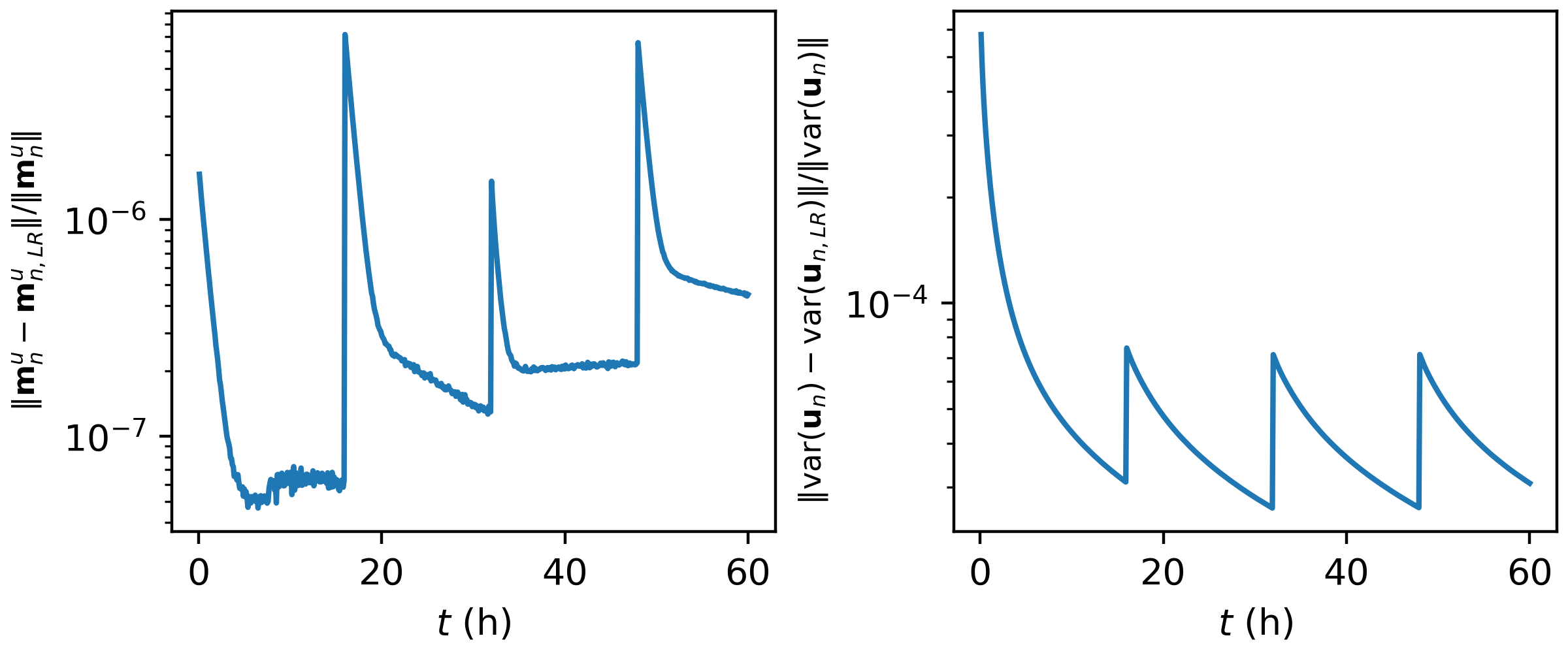
Figure 3: Relative error between the low-rank and full-rank ExKF, across all times, using $k=k^{\prime}=32$ modes, on the $u$ component.

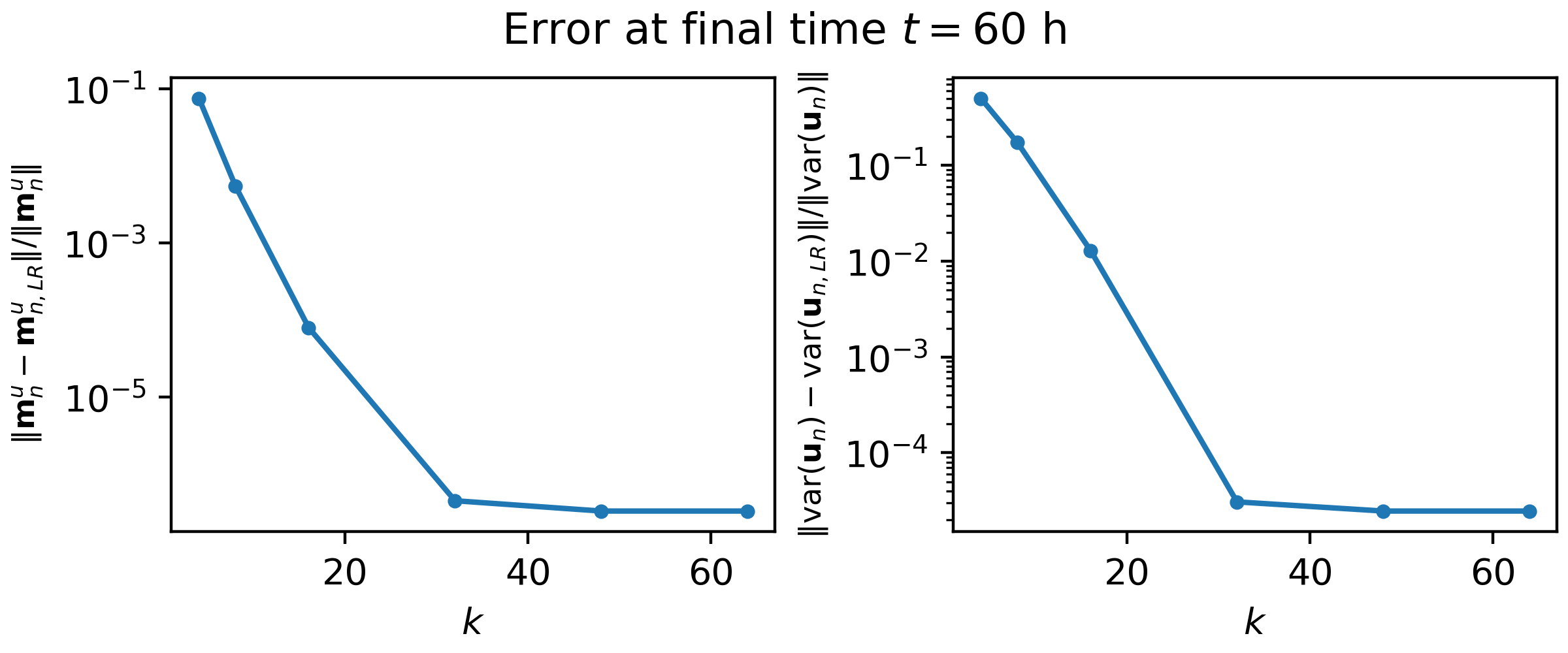
(a) Relative error between the low-rank and full-rank ExKF, at the final time $t=60$ h, as $k$ is increased ($k^{\prime}=32$ for all $k$).

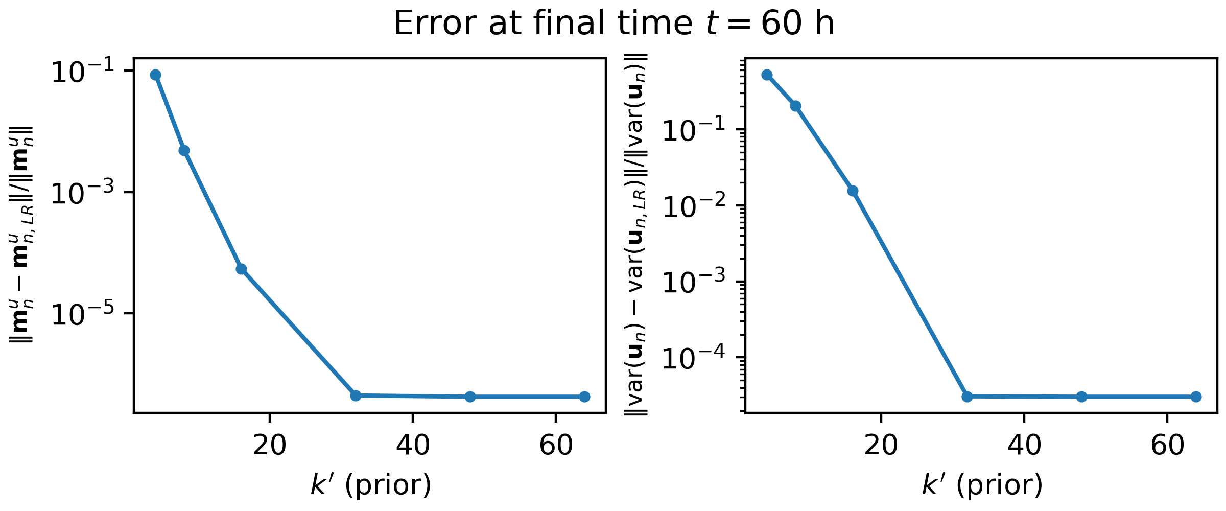
(b) Relative error between the low-rank and full-rank ExKF, at the final time $t=60$ h, as $k^{\prime}$ is increased ($k=32$ for all $k^{\prime}$).

Figure 4: Relative error comparisons between the low-rank and full-rank ExKF variants.

3.2 Mismatch via initial conditions: spiral regime

We now consider a two-dimensional example of misspecified initial conditions with the Oregonator [20, 21], a coupled PDE with state $\bm{w}=(u,v)\in\mathbb{R}^{2}$. Adding stochastic forcing on the observed $v$-component gives the two-dimensional system

$$\begin{cases}u_{t}=\frac{1}{\varepsilon}\left(u(1-u)-fv\frac{u-q}{u+q}\right)+D_{u}\nabla^{2}u,\\ v_{t}=u-v+D_{v}\nabla^{2}v+\xi_{v},\\ \nabla u\cdot\mathbf{n}=0,\quad\nabla v\cdot\mathbf{n}=0,\quad x\in\partial\Omega,\\ u:=u(\mathbf{x},t),\quad v:=v(\mathbf{x},t),\quad\mathbf{x}=(x_{1},x_{2})\in\Omega,\\ \Omega=[0,50]\times[0,50],\quad t\in[0,10].\end{cases}$$

The Oregonator has been well-studied after being derived as a simplified model for the chemical reaction kinetics of the Belousov-Zhabotinskii (BZ) reaction [20, 21, 42, 43]. It is a classical example of an activator-inhibitor system, sharing similar behaviour to the Fitzhugh-Nagumo model in certain parameter regimes [44]. We study the Oregonator in the excitable regime, setting $f=2$, $q=0.002$, and $\varepsilon=0.02$. Diffusion constants are set to $D_{u}=1$, $D_{v}=0.6$, The $\mathcal{GP}$ $\xi_{v}$ has the covariance kernel of Equation (2), setting $\bm{\theta}=(\rho,\ell)=(0.001,5)$.

Figure 5: Initial conditions on the $u$ component. StatFEM posterior initial condition shown on the left, and the true initial condition shown on the right.

To set the initial conditions, we use the procedure of [43]. To induce some degree of mismatch, initial conditions of the statFEM filtering posterior are set by pushing the initial condition of the truth through a heat equation with the diffusion coefficient $D_{u}=1$ (i.e. the Oregonator sans reaction terms), for $t=0.1$, resulting in the amplitude of the initial conditions being dampened and blurred (see Figure 5).

The spatial discretisation uses the standard linear polynomial hat functions, over a regular mesh with $128\times 128$ cells ($16,641$ nodes) so that the total state dimension is $33,282$ DOFs. Due to the nonlinear terms dominating the dynamics, Crank-Nicolson is used for time discretisation, with timesteps $\Delta_{t}=0.001$.

Data is observed on the slow $v$ component, at $1041$ locations inside the discretised domain $\Omega_{h}$. The time between observations is $0.005$ (5 timesteps). Data is sparse in space, having approximately $3\%$ of the state dimension observed at observation times, and the excitable $u$ is only updated through the observed $v$ values. As previous we concatenate the discretised state vector into $\mathbf{w}_{n}=(\mathbf{u}_{n}^{\top},\mathbf{v}_{n}^{\top})^{\top}$ so that the data generating process is $\mathbf{y}_{n}=\mathbf{H}\mathbf{w}_{n}+\bm{\eta}_{n}$, $\bm{\eta}_{n}\sim\mathcal{N}(0,\sigma^{2}\mathbf{I}_{n_{y}})$. The measurement fidelity is $\sigma=0.01$.

We run the LR-ExKF to obtain the posterior $p(\mathbf{w}_{n}\>|\>\mathbf{y}_{1:n},\bm{\theta},\sigma,\Lambda)=\mathcal{N}(\mathbf{m}_{n},\mathbf{L}_{n}\mathbf{L}_{n}^{\top})$ for all $n$, using $k=250$ ($\approx 0.75\%$ of the state dimension) modes to represent the state covariance $\mathbf{L}_{n}\mathbf{L}_{n}^{\top}$, and using $k^{\prime}=150$ modes to approximate the covariance matrix of $\xi_{v}$, $\mathbf{G}_{\theta}$. When running the filter, more than $99\%$ of the variance is retained at each truncation step.

To give a snapshot of results, the data, posterior mean, posterior variance, and leading order modes are each shown in Figure 6, at time $t=5$. The dominant region of variance appears to be at the spiral tip, with additional variation observed about the boundary of the spiral on the $u$ component. This hierarchy is seen in both the colour intensities of the variance plots in Figure 6(a) and in the columns of $\mathbf{L}_{n}$, in Figure 6(b); for UQ, there is a hierarchy of variance regions of decreasing importance.

(a) Top subplot: Posterior means $\mathbf{m}_{u}^{n}$ (top left), $\mathbf{m}_{v}^{n}$ (top centre), and observed data $\mathbf{y}_{n}$ (top right). Bottom subplot: posterior variances $\mathrm{var}(\mathbf{u}^{n})$ (bottom left) and $\mathrm{var}(\mathbf{v}^{n})$ (bottom right) (diagonal of the covariance matrix $\mathbf{L}_{n}\mathbf{L}_{n}^{\top}$). All are reported for time $t=5$.

(b) First eight columns of the posterior covariance square-root $\mathbf{L}_{n}$, for the $u$-component. These are the leading modes of variation at time $t=5$.

Figure 6: Posterior summary plots for time $t=5$ for the Oregonator spiral example.

Performance of the filter is verified through computing the relative errors on the means $\mathbf{m}_{n}^{u}$, $\mathbf{m}_{n}^{u}$ against the truth:

$$\frac{\lVert\mathbf{m}_{n}^{u}-\mathbf{u}_{n,\text{true}}\rVert}{\lVert\mathbf{u}_{n,\text{true}}\rVert},\quad\frac{\lVert\mathbf{m}_{n}^{v}-\mathbf{v}_{n,\text{true}}\rVert}{\lVert\mathbf{v}_{n,\text{true}}\rVert}.$$

These are shown in Figure 7(a). After an initial period of disparity, the statFEM mean $\mathbf{m}_{n}$ then closely tracks the truth, reaching a stable configuration after this initial warm-up period. Observations can thus correct for misspecification on the unobserved component, with small ($\mathcal{O}(10^{-2})$) relative errors in the mean of the statFEM posterior.

We also compute the effective rank $D_{\mathrm{eff}}$ [22, 23] of the prediction covariance matrix square-root $\hat{\mathbf{L}}_{n}$, using the eigenvalues from the truncation step. We define the effective rank from the eigenvalues (diagonal of $\bm{\Sigma}_{n}$) $\varsigma_{1}\geq\varsigma_{2}\geq\cdots\geq\varsigma_{k}$ of the $k\times k$ matrix $\hat{\mathbf{L}}_{n}^{\top}\hat{\mathbf{L}}_{n}$

$$D_{\mathrm{eff}}=\frac{\left(\sum_{i=1}^{k}\sqrt{\varsigma_{i}}\right)^{2}}{\sum_{i=1}^{k}\varsigma_{i}},$$

which takes values $D_{\text{eff}}\in[1,\min\{k,n_{u}\}]$. This measures the alignment of the columns of $\hat{\mathbf{L}}_{n}$ [22] and can be used to diagnose problems (for example filter collapse), or verify performance (for example, checking that $k$ and $k^{\prime}$ are not over- or under-specified). For this example, this is plotted in Figure 7(b), and appears to be stable after an initial drop, further suggesting that the filter has reached a stable configuration. The initial drop in the effective rank appears almost immediately after the filter is started, whereas for the relative errors this is at time $t=2$. This suggests that reaching a stable configuration in the covariance is perhaps necessary before the same occurs in the mean. The estimated $D_{\mathrm{eff}}$ has a mean value of approximately $D_{\mathrm{eff}}\approx 45$, indicating that the choice of $k=250$ is perhaps excessive for this example.

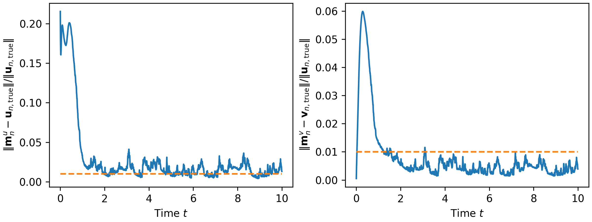
(a) Relative errors ${\lVert\mathbf{m}_{n}^{u}-\mathbf{u}_{n,\text{true}}\rVert}/{\lVert\mathbf{u}_{n,\text{true}}\rVert}$, and ${\lVert\mathbf{m}_{n}^{v}-\mathbf{v}_{n,\text{true}}\rVert}/{\lVert\mathbf{v}_{n,\text{true}}\rVert}$, for all times in the simulation.

(b) Effective rank of the prediction covariance square root $\hat{\mathbf{L}}_{n}$ for all times in the simulation.

Figure 7: Diagnostic plots for the spiral wave example.

3.3 Mismatch via initial conditions: oscillatory regime

In the oscillatory regime, the Oregonator has $f=0.95$, $\varepsilon=0.75$, $q=0.002$, and the diffusion coefficients $D_{u}=D_{v}=0.001$ [44]. Stochastic forcing is now included on the $u$ component

$$u_{t} =\frac{1}{\varepsilon}\left(u(1-u)-fv\frac{u-q}{u+q}\right)+D_{u}\nabla^{2}u+\xi_{u},$$

$$v_{t} =u-v+D_{v}\nabla^{2}v,$$

and the same spatio-temporal domain $\mathbf{x}\in\Omega=[0,50]\times[0,50]$, $t\in[0,10]$, is used. In this instance the initial conditions $(u_{0,\mathrm{true}},v_{0,\mathrm{true}})$ are perturbed via setting

$$u_{0}=u_{0,\mathrm{true}}+\varkappa\left(1+\sin\left(\frac{\pi x_{1}}{50}+\zeta_{1}\right)\sin\left(\frac{\pi x_{2}}{50}+\zeta_{2}\right)\right),\quad v_{0}=v_{0,\mathrm{true}},$$

where $\zeta_{1},\zeta_{2}\sim\mathcal{N}(0,1^{2})$, i.i.d. The amplitude $\varkappa$ is set to $0.02$ in our case studies, and for the true $(u_{0,\mathrm{true}},v_{0,\mathrm{true}})$, these are set from running a pilot simulation for $100,000$ timesteps, where the pilot simulation has randomly generated initial conditions $u,v\sim\mathrm{Unif}(0,0.15)$. The upper and lower bounds on the uniform distribution are determined from the attractor of the corresponding Oregonator ODE. Both the perturbed and true initial conditions are shown in Figure 8. This initial condition is included in the accompanying GitHub repository.

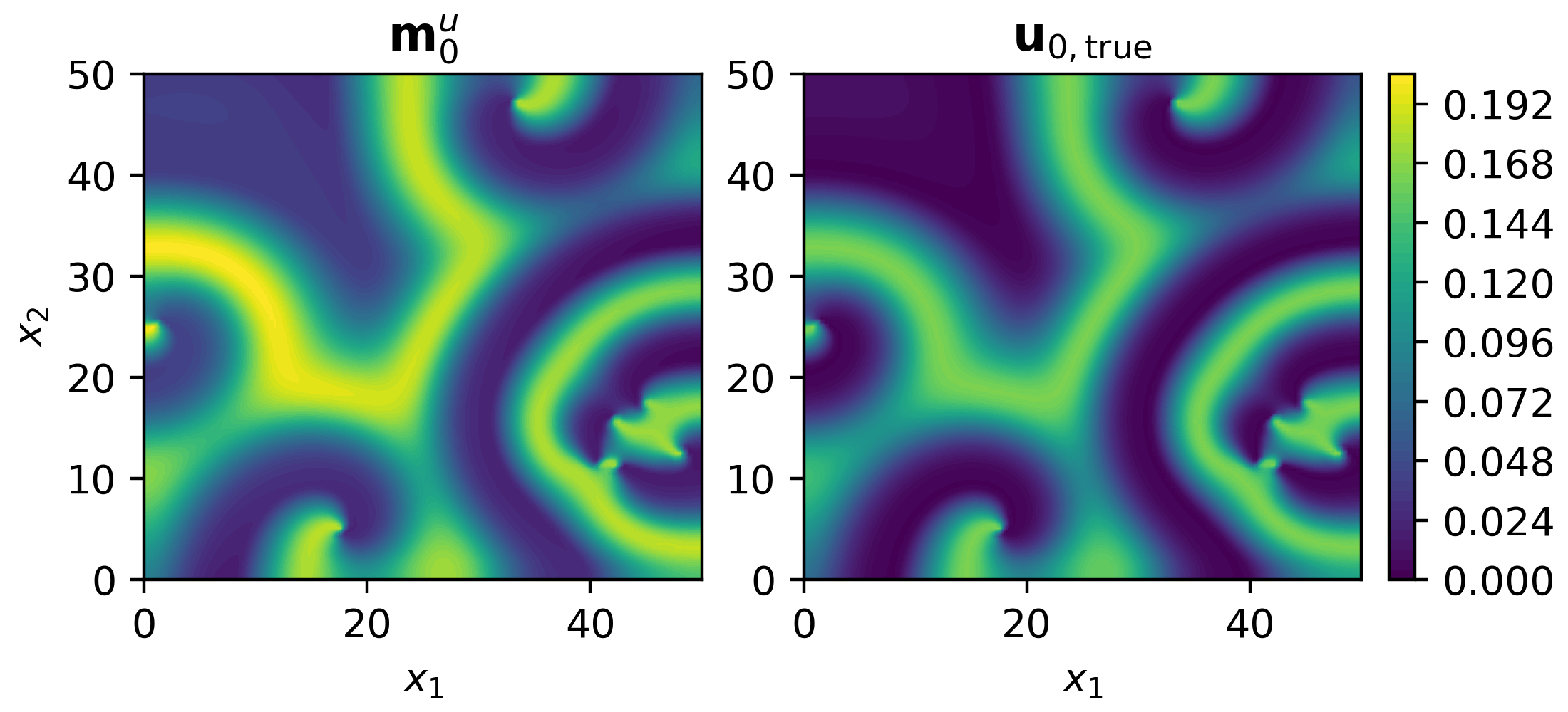
Figure 8: Initial conditions for $u$ component. StatFEM posterior initial condition shown on the left (same for each filter configuration) and the true initial conditions shown on the right.

As previous the spatial discretisation uses linear polynomial basis functions, on a refined mesh with $256\times 256$ cells. Crank-Nicolson is used for the time discretisation, with a timestep $\Delta_{t}=10^{-2}$, observing data $\mathbf{y}_{n}=\mathbf{H}\mathbf{w}_{n}+\bm{\eta}_{n}$ at every timestep up to time $t=10$. As previous, $\bm{\eta}_{n}\sim\mathcal{N}(0,\sigma^{2}\mathbf{I}_{n_{y}})$, with $\sigma=10^{-2}$, and the $u$-component is observed at each timestep, at $512$ observation locations. The posterior $p(\mathbf{w}_{n}\>|\>\mathbf{y}_{1:n},\bm{\theta},\sigma,\Lambda)=\mathcal{N}(\mathbf{m}_{n},\mathbf{L}_{n}\mathbf{L}_{n}^{\top})$ is computed using the LR-ExKF with $k=128$ and $k^{\prime}=64$. The initial leading-order eigendecomposition of the $\mathcal{GP}$ covariance matrix $\mathbf{G}_{\theta}$ is done using Lanczos iterations [29] as implemented in Scipy [39], with the matrix-vector products done on the GPU, implemented with KeOps [36].

We compare three filters, each with the $\mathcal{GP}$ covariance kernel of Equation (2), which set $\rho\in\{10^{-2},10^{-3},2\times 10^{-4}\}$, with $\ell=10$ and $\sigma=10^{-2}$ for each. In each filter more than $99\%$ of the variance is retained at each truncation step. For the remainder of this discussion these are referred to as the large-$\rho$ filter, the moderate-$\rho$ filter, and the small-$\rho$ filter, respectively.

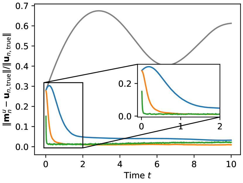
(a) Relative $l^{2}$ errors for the large-$\rho$, moderate-$\rho$, small-$\rho$ filters, and the prior model.

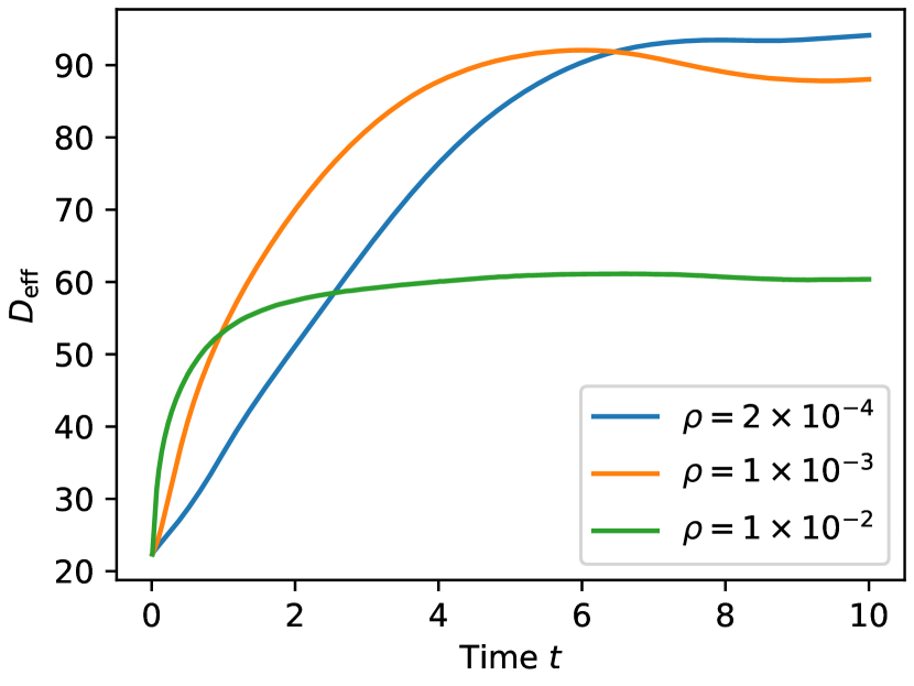
(b) Effective rank of the prediction covariance square root $\hat{\mathbf{L}}_{n}$ for the large-$\rho$, moderate-$\rho$, small-$\rho$ filters, and the prior model.

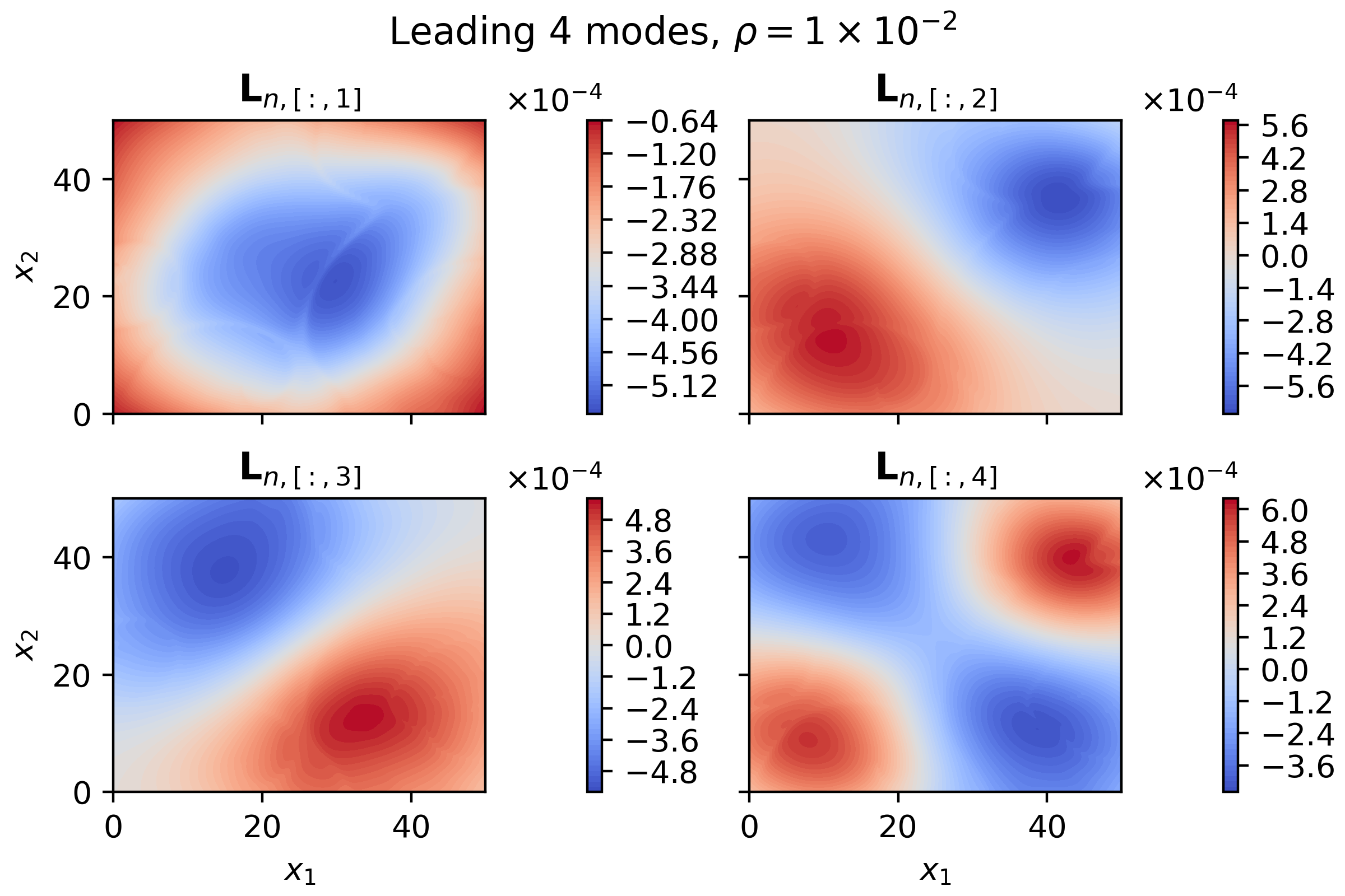
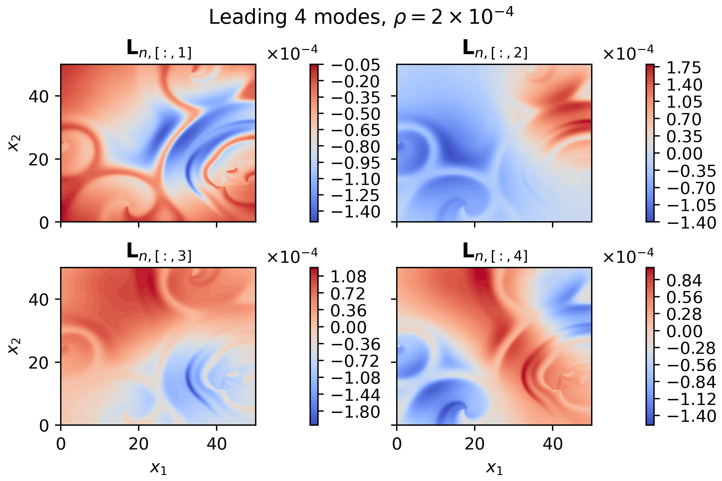
(c) Leading four covariance modes (first four columns of the posterior covariance matrix square root $\mathbf{L}_{n}$) for the large-$\rho$ filter (left, green ( ) in Figures 9(a) and 9(b)), and the small-$\rho$ filter (blue ( ) in Figures 9(a) and 9(b)). Shown are the modes for the $u$-component.

Figure 9: Relative $l^{2}$ errors (top left), effective rank $D_{\mathrm{eff}}$ (top right), and leading posterior covariance modes (bottom) at time $t=10$, oscillatory mismatched initial condition. The small-$\rho$ is shown in blue ( ), the moderate-$\rho$ in orange ( ), the large-$\rho$ in green ( ), and the prior model in grey ( ).

Relative errors for the statFEM posterior means are shown alongside the statFEM prior mean in Figure 9(a). The small-$\rho$ filter shows the slowest misspecification correction compared to the others; the filter is more certain of the model predictions and takes longer than the others to reach a stable filtering configuration. It also results in the largest relative error by the end of the simulation. The moderate $\rho$-filter, however, despite slower initial misspecification correction, results in the lowest relative error by $t=10$. The large-$\rho$ filter displays the most rapid convergence, yet results in relative errors increasing after the initial correction. This is thought to be due to $\rho$ being equal to the noise $\rho=\sigma=10^{-2}$, which results in assimilation of spurious noise perturbations. These results confirm the role of the $\rho$ hyperparameter in specifying our UQ of the physical model. Higher variance implies less certainty and more rapid corrections for model misspecification.

This trend of slower corrections, for more certain models, is also seen in the effective rank $D_{\mathrm{eff}}$ of the prediction covariance matrix $\hat{\mathbf{L}}_{n}\hat{\mathbf{L}}_{n}^{\top}$, plotted for each of the filters in Figure 9(b). In terms of $D_{\mathrm{eff}}$, the large-$\rho$ filter has the most rapid convergence to a stable filtering regime, with the small-$\rho$ filter the slowest. Once in this stable filtering regime the small-$\rho$ filter has a larger effective rank compared to the large-$\rho$ filter, and it is posited that a higher effective rank implies a more complex covariance structure. To check this the leading modes of the covariance matrix are plotted at the end time $t=10$, in Figure 9(c). The results suggests this is the case, and we see that the modes for the small-$\rho$ filter display more localised structures pertaining to the dynamics of the model, when compared with those of the large-$\rho$ filter, which appear more similar to the eigenfunctions of the $\mathcal{GP}$ covariance kernel $k_{\theta}(\cdot,\cdot)$.

This also merits another interpretation of the variance hyperparameter $\rho$: that of controlling the weight of the a priori misspecification covariance matrix $\mathbf{G}_{\theta}$ in comparison to the (tangent linear) dynamical evolution of the previous timestep covariance $\mathbf{C}_{n-1}=\mathbf{L}_{n-1}\mathbf{L}_{n-1}^{\top}$. In this case, due to the complex spatial oscillations seen in the dynamical model, by decreasing the weight of the simpler $\mathcal{GP}$ covariance, the more complex dynamical interactions are present in the posterior covariance, resulting in an increased $D_{\mathrm{eff}}$.

4 Conclusions

We present a low-rank extended Kalman filter algorithm for the statistical finite element method that is highly scalable, by representing the covariance matrix through its leading $k$ modes. Owing to the rapid spectral decay of this posterior covariance matrix the LR-ExKF is able to provide a sensible and interpretable UQ, retaining, in the given examples, at least $99\%$ of the variance at each timestep. Through the use of the Jacobian matrix (assembled from the Fréchet derivative of the weak form), the statFEM LR-ExKF is straightforward to implement with standard finite element libraries and has the potential for massive parallelisation in the bottleneck prediction step.

We demonstrate, using experimental and synthetic data, that statFEM is able to combine models and data in a coherent statistical framework, correcting for model misspecification in various forms. Results in 1D, with experimental data, show that the LR-ExKF can approximate the full-rank alternative, with small relative errors in both the posterior mean and variance. These results also confirm the efficacy of statFEM in the face of temporally sparse observation regimes. Results with the 2D Oregonator system demonstrate scalability, with the statFEM LR-ExKF correcting for model misspecification in the initial conditions, through observing a single component of the underlying data-generating process. These results are robust under different model parameter regimes, and, under increasing the state dimension to $n_{u}=132,098$. We also show that the effective rank of the covariance matrix can verify the number of modes taken in the low-rank approximation, providing an additional check of filter convergence.

This work provides a scalable statFEM that will enable the application of the methodology to domains across the physical sciences. Our method is similar to the EnKF, representing the covariance matrix through a low-rank approximation (c.f. D), though by using the leading eigenvalues and eigenvectors we ensure that the UQ is empirically justified. An additional source of uncertainty that is not considered in this work is that of the hyperparameters, $\bm{\theta}$, which would ideally be marginalised over [45]. The investigation of this estimation approach would be of interest.

Additional extensions to this work include verifying that the LR-ExKF produces accurate estimates of the true filtering posterior, and theoretical work to check the accuracy and stability of the filter. Furthermore, when applying to arbitrary time-dependent PDEs one may require the use of bespoke timestepping schemes, going beyond the Crank-Nicolson scheme used in this paper. One may also need to constrain the timesteps to ensure that the tangent linear approximation to the covariance matrix does not induce too much error or to control for possible filter divergence. An iterative extension may also be required for sufficiently nonlinear PDEs [46].

Appendix A Notes on numerics

All results in this paper were obtained on a workstation PC with an i7-6850k CPU, equipped with 64GB of memory, and an nVidia GTX 1080 Ti GPU. All finite element computations (i.e. matrix assembly and automatic differentiation for the Jacobian) are handled with Fenics [41]. At each timestep, when solving the nonlinear system, we use the standard Newtons method, as implemented in PETSc, using the LU decomposition to solve the linear system at each Newton step. When performing the covariance propagation, i.e. solving systems of the form

$$(\mathbf{M}+\Delta_{t}\kappa\mathbf{A}+\Delta_{t}D_{n}\tilde{\mathbf{r}})^{-1}\mathbf{X},\quad\mathbf{X}\in\mathbb{R}^{n_{u}\times p},$$

we again employ the LU factorization so as to reuse the factors.

We construct the matrix $\mathbf{G}_{\theta}$ through approximation, using $\mathbf{G}_{\theta}=\mathbf{M}\mathbf{K}_{\theta}\mathbf{M}^{\top}$, for the mass matrix $\mathbf{M}$ and the squared-exponential matrix $\mathbf{K}_{\theta,ij}=k_{\theta}(x_{i},x_{j})$ (see the supplement of [2] for further details). The low-rank approximation $\mathbf{G}_{\theta}^{1/2}$ is computed using the leading $k^{\prime}$ modes of $\mathbf{K}_{\theta}$, which, depending on the problem at hand, are computed using vanilla Scipy (on the CPU) or with KeOps (on the GPU). This gives $\mathbf{G}_{\theta}^{1/2}=\mathbf{M}\mathbf{K}_{\theta}^{1/2}$.

Appendix B Influence of prior modes in the cell example

As discussed in the main text (Section 3.1), in the cell example, the prior modes control the accuracy of the UQ given by the LR-ExKF. Here we investigate this further, through checking the errors in the posterior mean and variance as we vary the prior modes $k^{\prime}$ and the observational noise $\sigma$. For each $k^{\prime}$ we fix the filter modes $k$ to $k=k^{\prime}+16$, to allow for sufficient extra modes to capture information present in the data, not included in the prior modes. Note that in this instance the variation of $\sigma$ is only to investigate the computational performance of the filtering method; the known noise value of $\sigma=10^{-2}$ should be used (as it is in the main text) when attempting to infer the system state from measurements.

The results of running the filters for $k^{\prime}\in\{16,32,48,64\}$, $\sigma\in\{10^{-4},10^{-3},10^{-2},10^{-1}\}$ are shown in Figure 10. These suggest that as the noise decreases (i.e., the data becomes more informative) then more modes are required to accurately capture the variance. Despite the additional “overhead modes” on $k=k^{\prime}+16$, gains are seen when increasing $k^{\prime}$, confirming that the number of prior modes have a large affect on the performance on the filter. Errors in the posterior mean appear to increase more rapidly with the decreasing $\sigma$, in comparison to the variance. It is posited that this discrepancy is seen due to the posterior mean update using the full nonlinear dynamics when completing the prediction step — the covariance propagation, in comparison, uses the tangent linear dynamics.

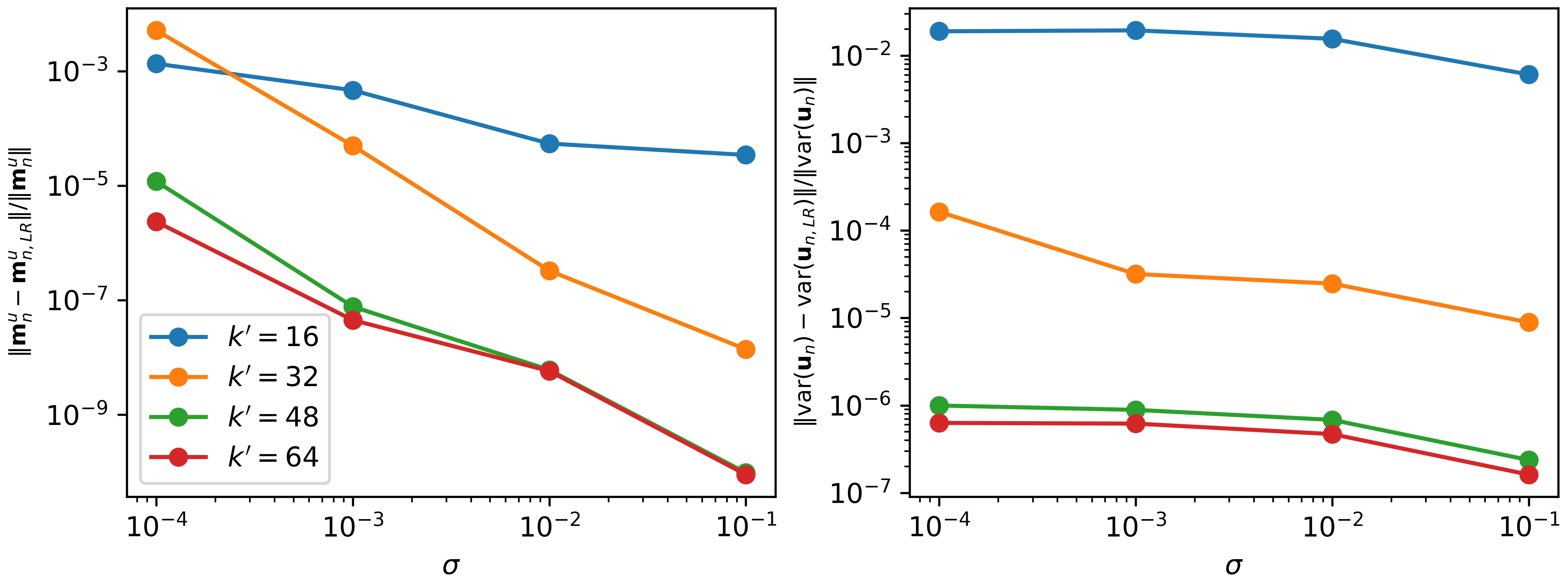
Figure 10: Relative errors on the posterior mean (left) and variance (right) as both the number of prior modes ($k^{\prime}$) and observation noise ($\sigma$) is increased.

Appendix C Verification of parameter estimation

For this example, the Oregonator equations in the oscillatory regime are used (recall $f=0.95$, $\varepsilon=0.75$, $q=0.002$, and the diffusion coefficients $D_{u}=D_{v}=0.001$ [44]). Data is generated according to a stochastic Oregonator with stochastic forcing on the $u$ component

$$u_{t} =\frac{1}{\varepsilon}\left(u(1-u)-fv\frac{u-q}{u+q}\right)+D_{u}\nabla^{2}u+\xi_{u},$$

$$v_{t} =u-v+D_{v}\nabla^{2}v,$$

and we verify the proposed hyperparameter estimation routine of Section 2.

Figure 11: FEM mesh (blue) and observation locations (orange), for C.

Initial conditions are the same as for the previous oscillatory example, and the same space-time domain is used as previous: $\mathbf{x}\in\Omega=[0,50]\times[0,50]$, $t\in[0,10]$. Timesteps use an implicit-explicit (IMEX) scheme [26] with forward and backward Euler:

$$\mathbf{M}\left(\mathbf{w}_{n+1}-\mathbf{w}_{n}\right)+\Delta_{t}\kappa\mathbf{A}\mathbf{w}_{n+1}=\Delta_{t}\tilde{\mathbf{r}}(\mathbf{w}_{n})+\mathbf{e}_{n},$$

recalling the concatenated state $\mathbf{w}_{n}=(\mathbf{u}_{n}^{\top},\mathbf{v}_{n}^{\top})^{\top}$. Timestep size is set to $\Delta_{t}=10^{-2}$ or $\Delta_{t}=10^{-4}$, and we investigate the accuracy of the estimated hyperparameters for each (each filter is run for $1000$ timesteps). Note that this does not yield the same integration window, one being two orders of magnitude smaller than the other.

Data, of the $u$ component is observed at $512$ locations at each timestep (locations shown in Figure 11). The assumed data generating process is $\mathbf{y}_{n}=\mathbf{H}\mathbf{w}_{n}+\bm{\eta}_{n}$, $\bm{\eta}_{n}\sim\mathcal{N}(\mathbf{0},\sigma^{2}\mathbf{I}_{n_{y}})$. Data is generated with $\sigma=0.01$, and $\bm{\theta}=(\rho,\ell)=(10^{-3},10)$. Filtering is done using LR-ExKF, with $k=k^{\prime}=128$ modes, to compute the posterior $p(\mathbf{w}_{n}\>|\>\mathbf{y}_{1:n},\bm{\theta}_{1:n},\sigma_{1:n},\Lambda)\sim\mathcal{N}(\mathbf{m}_{n},\mathbf{L}_{n}\mathbf{L}_{n}^{\top})$. For the various filters in this section, each retain at least $99\%$ of the variance at each timestep. The leading eigenvalues of $\mathbf{K}_{\theta}$, which determine the accuracy of the low-rank approximation $\mathbf{G}_{\theta}^{1/2}$, are shown in Figure 12, and have a range of approximately $(10^{-4},10^{3})$.

To avoid recomputing $\mathbf{G}_{\theta}$ at each iteration, $\ell$ is fixed at $\ell=10$ for all $n$, and we estimate $\rho_{n}$ and $\sigma_{n}$ at each $n$, assuming that $\rho_{n}$ and $\sigma_{n}$ are independent for each $n$. Incorporating more complex temporal structure on these hyperparameters is of interest and is a possible avenue for future research. Priors are set to the weakly informative Gaussian priors $\rho_{n}\sim\mathcal{N}_{+}(1,1^{2})$ and $\sigma_{n}\sim\mathcal{N}_{+}(0,1^{2})$.

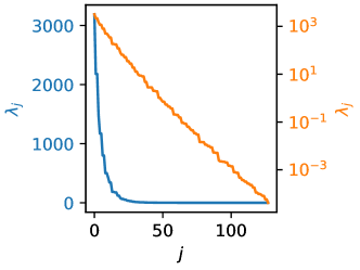
Figure 12: Leading $128$ eigenvalues of $\mathbf{G}_{\theta}$ (for C).

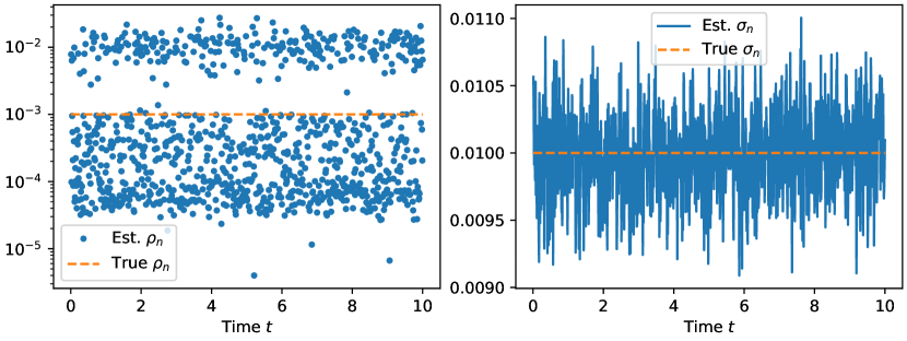
(a) Estimated hyperparameters $\rho_{n}$ and $\sigma_{n}$, across all times, running the filter with $\Delta_{t}=10^{-2}$.

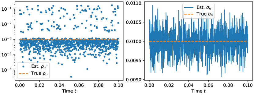
(b) Estimated hyperparameters $\rho_{n}$ and $\sigma_{n}$, across all times, now running the filter with $\Delta_{t}=10^{-4}$.

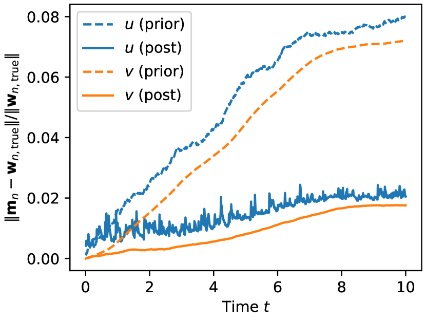
(c) Relative $l^{2}$ errors on the $u$ (blue) and $v$ (orange) components, for the prior (dashed line) and the posterior (solid line), using $\Delta_{t}=10^{-2}$.

(d) Effective rank $D_{\mathrm{eff}}$ of the prediction covariance $\hat{L}_{n}\hat{L}_{n}^{\top}$ using $\Delta_{t}=10^{-2}$.

Figure 13: Diagnostic plots for the stochastic forcing example.

The hyperparameter estimates are shown in Figures 13(a) and 13(b), and demonstrate that the noise is identified at each timestep. For the larger timestep $\Delta_{t}=10^{-2}$ the hyperparameter $\rho_{n}$ is poorly identified. Estimates appear to be contained within two point clouds, the topmost cloud being identified with the noise $\sigma_{n}$. This inaccuracy is thought to be due to the combination of linearized dynamics for the covariance update combined with the low-rank approximation for the square root $\mathbf{G}_{\theta}$. Note also that the inclusion of the truncated Gaussian prior $\rho_{n}\sim\mathcal{N}_{+}(1,1)$ will also have an effect.

This is confirmed by running the same filter with the smaller timestep $\Delta_{t}=10^{-4}$, thought to increase the accuracy of the linearised covariance prediction step. The filter appears to better identify the scale hyperparameter $\rho_{n}$ (see Figure 13(b)). Some variation remains, however, which is thought to be due to the low-rank approximation to $\mathbf{G}_{\theta}$ and the truncated Gaussian prior. For completeness we also plot the relative $l^{2}$ errors in Figure 13(c) and the effective rank of the covariance matrix in Figure 13(d). We see that the variation of the effective rank appears to be due to the variation in the estimates of the hyperparameters (c.f. the smooth effective rank results seen in the main text for fixed hyperparameter values).

Appendix D Catastrophic filter divergence in the spiral wave regime

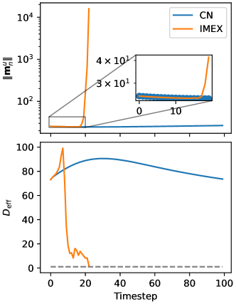
Figure 14: Norm of the statFEM posterior mean $m_{n}$ for the $u$-component (top), and effective rank $D_{\mathrm{eff}}$ (bottom).

In this case study we show that the LR-ExKF can have catastrophic filter divergence occur, which is also observed with the EnKF [22, 47]. Catastrophic filter divergence is where the posterior mean estimate $\mathbf{m}_{n}$ diverges to machine infinity in finite time. Previous studies are contextually similar, with EnKF divergence occurring in sparsely observed dissipative nonlinear systems with small noise. The mechanism of the divergence is the use of an unstable time-integration scheme [22], which we verify.

We simulate data according to a deterministic Oregonator in the spiral wave regime (recall $f=2$, $q=0.002$, and $\varepsilon=0.02$). These data are observed at every timestep, on the slow $v$ component, across $512$ observation locations. The initial conditions are the same as those in the second case study in the main text. Additive Gaussian noise is added, so that $\mathbf{y}_{n}=\mathbf{H}\mathbf{w}_{n}+\bm{\eta}_{n}$, $\bm{\eta}_{n}\sim\mathcal{N}(\mathbf{0},10^{-4}\mathbf{I}_{n_{y}})$. There is no model mismatch between the statFEM model and the underlying data generating process for $\mathbf{y}_{n}$; the only difference is that the statFEM model includes the stochastic process $\xi_{v}$ on the component $v$, which has the covariance kernel of Equation (2). $\mathcal{GP}$ hyperparameters are fixed, with $\bm{\theta}=(\rho,\ell)=(10^{-3},10)$. For the numerics, both models use an FEM mesh with $128\times 128$ cells, and the timestep size is $\Delta_{t}=10^{-3}$.

Filtering is done using the LR-ExKF, with $k=512$ and $k^{\prime}=128$ modes, to compute the posterior $p(\mathbf{w}_{n}\>|\>\mathbf{y}_{1:n},\bm{\theta},\sigma,\Lambda)\sim\mathcal{N}(\mathbf{m}_{n},\mathbf{L}_{n}\mathbf{L}_{n}^{\top})$. For each filter more than $99\%$ of the variance is retained at each timestep.. We say that the filter has diverged if any of elements $\mathbf{u}_{n,i}\geq 10^{4}$ for $i=1,\ldots,n_{u}$, and two separate filters are run: one with the IMEX scheme of C for timesteps, and the other with the Crank-Nicolson (CN) scheme for timesteps.

The IMEX filter diverges to machine infinity after $23$ timesteps (see Figure 14, top). The proposed mechanism of this divergence is that the posterior estimates of the mean do not accord with the underlying attractor, resulting in stiffness in the underlying dynamical model [22]. Hence the time integration becomes stiff, which the IMEX scheme is not able to resolve, and the filter diverges. In [22] this is accompanied by the effective rank of the covariance matrix reducing to one, which gives spurious correlations and thus poor posterior estimates in the update step. This is observed in this scenario, too, with the effective rank dropping to near unity in finite time by the divergent timestep $n=23$. Note also the resemblance to particle filter degeneracy, which results in the collapse of the particle weights to a Dirac measure.

As in examples in the main text, the behaviour of the relative norm also “lags” the behaviour of the effective rank; the effective rank seems to drop sharply whilst the relative norms of the IMEX and CN are both visually indistinguishable. Only after the effective rank drops to near unity is the divergence seen, giving a reminder of the influence of the posterior covariance matrix $\mathbf{C}_{n}$ on posterior estimates of the mean $\mathbf{m}_{n}$. Changing the time integrator to CN results in catastrophic filter divergence being avoided, and the relative $l^{2}$ norm and $D_{\text{eff}}$ appear to asymptotically approach some limiting value after an initial increase (see Figure 14). Note also the smoothness of the effective rank $D_{\mathrm{eff}}$ resulting from the fixed choice of hyperparameter $\rho$.

References

- [1] M. Girolami, E. Febrianto, G. Yin, F. Cirak, The statistical finite element method (statFEM) for coherent synthesis of observation data and model predictions, Computer Methods in Applied Mechanics and Engineering 375 (2021) 113533. doi:10.1016/j.cma.2020.113533.
- [2] C. Duffin, E. Cripps, T. Stemler, M. Girolami, Statistical finite elements for misspecified models, Proceedings of the National Academy of Sciences 118 (2) (Jan. 2021). doi:10.1073/pnas.2015006118.
- [3] S. H. Rudy, S. L. Brunton, J. L. Proctor, J. N. Kutz, Data-driven discovery of partial differential equations, Science Advances 3 (4) (2017) e1602614. doi:10.1126/sciadv.1602614.
- [4] S. L. Brunton, J. L. Proctor, J. N. Kutz, Discovering governing equations from data by sparse identification of nonlinear dynamical systems, Proceedings of the National Academy of Sciences 113 (15) (2016) 3932–3937. doi:10.1073/pnas.1517384113.
- [5] M. Raissi, P. Perdikaris, G. E. Karniadakis, Physics-informed neural networks: A deep learning framework for solving forward and inverse problems involving nonlinear partial differential equations, Journal of Computational Physics 378 (2019) 686–707. doi:10.1016/j.jcp.2018.10.045.
- [6] Y. Bar-Sinai, S. Hoyer, J. Hickey, M. P. Brenner, Learning data-driven discretizations for partial differential equations, Proceedings of the National Academy of Sciences 116 (31) (2019) 15344–15349. doi:10.1073/pnas.1814058116.
- [7] M. Raissi, G. E. Karniadakis, Hidden physics models: Machine learning of nonlinear partial differential equations, Journal of Computational Physics 357 (2018) 125–141. doi:10.1016/j.jcp.2017.11.039.
- [8] C. K. Williams, C. E. Rasmussen, Gaussian Processes for Machine Learning, Vol. 2, MIT press Cambridge, MA, 2006.
- [9] A. M. Stuart, Inverse problems: A Bayesian perspective, Acta Numerica 19 (2010) 451–559. doi:10.1017/S0962492910000061.
- [10] K. Law, A. Stuart, K. Zygalakis, Data Assimilation: A Mathematical Introduction, Vol. 62, Springer, Cham, Switerland, 2015.
- [11] M. Verlaan, A. W. Heemink, Tidal flow forecasting using reduced rank square root filters, Stochastic Hydrology and Hydraulics 11 (5) (1997) 349–368. doi:10.1007/BF02427924.
- [12] S. Gillijns, D. Bernstein, B. De Moor, The Reduced Rank Transform Square Root Filter for Data Assimilation, IFAC Proceedings Volumes 39 (1) (2006) 1252–1257. doi:10.3182/20060329-3-AU-2901.00202.
- [13] D. Rozier, F. Birol, E. Cosme, P. Brasseur, J. M. Brankart, J. Verron, A Reduced-Order Kalman Filter for Data Assimilation in Physical Oceanography, SIAM Review 49 (3) (2007) 449–465. doi:10.1137/050635717.
- [14] K. J. H. Law, A. M. Stuart, Evaluating Data Assimilation Algorithms, Monthly Weather Review 140 (11) (2012) 3757–3782. doi:10.1175/MWR-D-11-00257.1.
- [15] A. Doucet, S. Godsill, C. Andrieu, On sequential Monte Carlo sampling methods for Bayesian filtering, Statistics and Computing 10 (3) (2000) 197–208. doi:10.1023/A:1008935410038.
- [16] G. Evensen, The Ensemble Kalman Filter: Theoretical formulation and practical implementation, Ocean Dynamics 53 (4) (2003) 343–367. doi:10.1007/s10236-003-0036-9.
- [17] T. Bengtsson, P. Bickel, B. Li, Curse-of-dimensionality revisited: Collapse of the particle filter in very large scale systems, Probability and Statistics: Essays in Honor of David A. Freedman (2008) 316–334doi:10.1214/193940307000000518.
- [18] V. Thomée, Galerkin Finite Element Methods for Parabolic Problems, 2nd Edition, no. v. 25 in Springer Series in Computational Mathematics, Springer, Berlin ; New York, 2006.
- [19] R. E. Kalman, A New Approach to Linear Filtering and Prediction Problems, Journal of Basic Engineering 82 (1) (1960) 35–45. doi:10.1115/1.3662552.
- [20] R. J. Field, E. Koros, R. M. Noyes, Oscillations in chemical systems. II. Thorough analysis of temporal oscillation in the bromate-cerium-malonic acid system, Journal of the American Chemical Society 94 (25) (1972) 8649–8664. doi:10.1021/ja00780a001.
- [21] J. J. Tyson, P. C. Fife, Target patterns in a realistic model of the Belousov–Zhabotinskii reaction, The Journal of Chemical Physics 73 (5) (1980) 2224–2237. doi:10.1063/1.440418.
- [22] G. A. Gottwald, A. J. Majda, A mechanism for catastrophic filter divergence in data assimilation for sparse observation networks, Nonlinear Processes in Geophysics 20 (5) (2013) 705–712. doi:10.5194/npg-20-705-2013.
- [23] D. J. Patil, B. R. Hunt, E. Kalnay, J. A. Yorke, E. Ott, Local Low Dimensionality of Atmospheric Dynamics, Physical Review Letters 86 (26) (2001) 5878–5881. doi:10.1103/PhysRevLett.86.5878.
- [24] K. P. Murphy, Machine Learning: A Probabilistic Perspective, Adaptive Computation and Machine Learning Series, MIT Press, Cambridge, MA, 2012.
- [25] G. Da Prato, J. Zabczyk, Stochastic Equations in Infinite Dimensions, 2nd Edition, Encyclopedia of Mathematics and Its Applications, Cambridge University Press, Cambridge, 2014. doi:10.1017/CBO9781107295513.
- [26] U. M. Ascher, S. J. Ruuth, B. T. R. Wetton, Implicit-Explicit Methods for Time-Dependent Partial Differential Equations, SIAM Journal on Numerical Analysis 32 (3) (1995) 797–823.
- [27] P. Kloeden, E. Platen, Numerical Solution of Stochastic Differential Equations, Applications of Mathematics, Springer Berlin Heidelberg, 1992.
- [28] G. H. Golub, C. F. Van Loan, Matrix Computations, JHU Press, 2013.
- [29] Y. Saad, Iterative Methods for Sparse Linear Systems, Other Titles in Applied Mathematics, Society for Industrial and Applied Mathematics, 2003. doi:10.1137/1.9780898718003.
- [30] G. Evensen, Data Assimilation: The Ensemble Kalman Filter, 2nd Edition, Springer-Verlag, Berlin Heidelberg, 2009. doi:10.1007/978-3-642-03711-5.
- [31] A. Banerjee, J. Vogelstein, D. Dunson, Parallel inversion of huge covariance matrices, arXiv:1312.1869 [stat] (Dec. 2013). arXiv:1312.1869.
- [32] R. Zimmermann, On the condition number anomaly of Gaussian correlation matrices, Linear Algebra and its Applications 466 (2015) 512–526. doi:10.1016/j.laa.2014.10.038.
- [33] Y. Saatci, Scalable Inference for Structured Gaussian Process Models, Ph.D. thesis, University of Cambridge (2011).
- [34] C. R. Dietrich, G. N. Newsam, Fast and Exact Simulation of Stationary Gaussian Processes through Circulant Embedding of the Covariance Matrix, SIAM Journal on Scientific Computing 18 (4) (1997) 1088–1107. doi:10.1137/S1064827592240555.
- [35] A. Solin, S. Särkkä, Hilbert space methods for reduced-rank Gaussian process regression, Statistics and Computing 30 (2) (2020) 419–446. doi:10.1007/s11222-019-09886-w.
- [36] B. Charlier, J. Feydy, J. A. Glaunès, F.-D. Collin, G. Durif, Kernel Operations on the GPU, with Autodiff, without Memory Overflows, Journal of Machine Learning Research 22 (74) (2021) 1–6.
- [37] J. Mandel, Efficient Implementation of the Ensemble Kalman Filter, University of Colorado at Denver and Health Sciences Center, Center for Computational Mathematics (2006) 9.
- [38] J. Nocedal, S. Wright, Numerical Optimization, Springer Science & Business Media, 2006.
- [39] P. Virtanen, R. Gommers, T. E. Oliphant, M. Haberland, T. Reddy, D. Cournapeau, E. Burovski, P. Peterson, W. Weckesser, J. Bright, S. J. van der Walt, M. Brett, J. Wilson, K. Jarrod Millman, N. Mayorov, A. R. J. Nelson, E. Jones, R. Kern, E. Larson, C. Carey, İ. Polat, Y. Feng, E. W. Moore, J. Vand erPlas, D. Laxalde, J. Perktold, R. Cimrman, I. Henriksen, E. A. Quintero, C. R. Harris, A. M. Archibald, A. H. Ribeiro, F. Pedregosa, P. van Mulbregt, S. . . Contributors, SciPy 1.0: Fundamental Algorithms for Scientific Computing in Python, Nature Methods 17 (3) (2020) 261–272. doi:10.1038/s41592-019-0686-2.
- [40] M. J. Simpson, R. E. Baker, S. T. Vittadello, O. J. Maclaren, Practical parameter identifiability for spatio-temporal models of cell invasion, Journal of The Royal Society Interface 17 (164) (2020) 20200055. doi:10.1098/rsif.2020.0055.
- [41] A. Logg, K.-A. Mardal, G. Wells, Automated Solution of Differential Equations by the Finite Element Method: The FEniCS Book, Vol. 84, Springer Science & Business Media, 2012.
- [42] R. J. Field, R. M. Noyes, Oscillations in chemical systems. IV. Limit cycle behavior in a model of a real chemical reaction, The Journal of Chemical Physics 60 (5) (1974) 1877–1884. doi:10.1063/1.1681288.
- [43] W. Jahnke, W. E. Skaggs, A. T. Winfree, Chemical vortex dynamics in the Belousov-Zhabotinskii reaction and in the two-variable oregonator model, The Journal of Physical Chemistry 93 (2) (1989) 740–749. doi:10.1021/j100339a047.
- [44] Y. Gong, D. J. Christini, Antispiral Waves in Reaction-Diffusion Systems, Physical Review Letters 90 (8) (2003) 088302. doi:10.1103/PhysRevLett.90.088302.
- [45] M. Filippone, M. Girolami, Pseudo-Marginal Bayesian Inference for Gaussian Processes, IEEE Transactions on Pattern Analysis and Machine Intelligence 36 (11) (2014) 2214–2226. arXiv:1310.0740, doi:10.1109/TPAMI.2014.2316530.
- [46] P. Sakov, D. S. Oliver, L. Bertino, An Iterative EnKF for Strongly Nonlinear Systems, Monthly Weather Review 140 (6) (2012) 1988–2004. doi:10.1175/MWR-D-11-00176.1.
- [47] J. Harlim, A. J. Majda, Catastrophic filter divergence in filtering nonlinear dissipative systems, Communications in Mathematical Sciences 8 (1) (2010) 27–43. doi:cms/1266935012.