Worldtube excision method for intermediate-mass-ratio inspirals: scalar-field toy model

Abstract

The computational cost of inspiral and merger simulations for black-hole binaries increases in inverse proportion to the square of the mass ratio $q:=m_{2}/m_{1}\leq 1$. One factor of $q$ comes from the number of orbital cycles, which is proportional to $1/q$, and another is associated with the required number of time steps per orbit, constrained (via the Courant-Friedrich-Lewy condition) by the need to resolve the two disparate length scales. This problematic scaling makes simulations progressively less tractable at smaller $q$. Here we propose and explore a method for alleviating the scale disparity in simulations with mass ratios in the intermediate astrophysical range ($10^{-4}\lesssim q\lesssim 10^{-2}$), where purely perturbative methods may not be adequate. A region of radius much larger than $m_{2}$ around the smaller object is excised from the numerical domain, and replaced with an analytical model approximating a tidally deformed black hole. The analytical model involves certain a priori unknown parameters, associated with unknown bits of physics together with gauge-adjustment terms; these are dynamically determined by matching to the numerical solution outside the excision region. In this paper we develop the basic idea and apply it to a toy model of a scalar charge in a circular geodesic orbit around a Schwarzschild black hole, solving for the massless Klein-Gordon field in a 1+1D framework. Our main goal here is to explore the utility and properties of different matching strategies, and to this end we develop two independent implementations, a finite-difference one and a spectral one. We discuss the extension of our method to a full 3D numerical evolution and to gravity.

I Introduction

All gravitational-wave signals reported so far by the LIGO-Virgo Collaboration [1, 2] originated from compact-object binaries in which the two components had fairly comparable masses. The most extreme mass disparity to date was observed in GW190814, whose likely source was the coalescence of a $2.50$–$2.67M_{\odot}$ object (either an exceptionally heavy neutron star or an exceptionally light black hole) with a $22.2$–$24.3M_{\odot}$ black hole [3]. Upgrades and future generations of ground-based detectors [4, 5], and especially the planned space-based detector LISA [6], will open up a new window of observation in the low-frequency band of the gravitational-wave spectrum, enabling the detection of signals from ever heavier binary systems, including ones containing intermediate-mass and supermassive black holes. In consequence, it is expected that the detection of high mass ratio events will become routine, and that the catalogue of detected binary sources will extend to include a broad range of mass ratios—potentially down to $\sim 1$:$10^{6}$ with LISA [7, 8, 9].

In anticipation of this remarkable expansion in observational reach, it is important to develop accurate theoretical waveform templates that reliably cover the entire relevant range of mass ratios. Standard Numerical Relativity (NR) methods [10] work well for mass ratios in the range $0.1\lesssim q:=m_{2}/m_{1}\leq 1$ (see e. g. [11]). However, simulations become progressively less tractable at smaller $q$, and few numerical simulations have been performed at $q<0.1$ so far. The root cause is a problematic scaling of the required simulation time with $q$. Fundamentally, one expects the required simulation time to grow in proportion to $q^{-2}$, where one factor of $q^{-1}$ is associated with the number of in-band orbital cycles, and the second factor $q^{-1}$ comes from the Courant-Friedrich-Lewy (CFL) stability limit on the time step of the numerical simulation, constrained by the need to spatially resolve the small object. The state of the art in small-$q$ NR is represented by the recent simulations performed at RIT of the last 13 orbital cycles prior to merger of a black-hole binary system with $q=1/128$ [12, 13]. Such simulations remain extremely computationally expensive.

For extreme mass ratios (say, $q\lesssim 10^{-4}$), it is more natural to apply an alternative treatment based on black-hole perturbation theory. Here, the field equations are formally expanded in powers of $q$, and the orbital dynamics are described in terms of a point-particle inspiral trajectory on the fixed geometry of the large black hole. In the limit $q\to 0$, the trajectory is geodesic. Back reaction from the small object’s self-field, which drives the slow inspiral, is accounted for order-by-order in $q$, in what is known as the gravitational self-force (GSF) approach [14, 15]. GSF is currently the only viable method for modelling astrophysical extreme-mass-ratio inspirals (EMRIs), in which a compact object orbits a massive black hole in a galactic nucleus. Development continues towards an accurate model of EMRI waveforms suitable for signal identification and interpretation with LISA [16, 17, 18, 19, 20, 21].

The intermediate range of mass ratios, say $10^{-4}\lesssim q\lesssim 10^{-1}$, poses a unique modelling challenge. A priori, it is hard to ascertain whether GSF calculations can in practice cover with sufficient accuracy the entire range of $q$ where the computational cost of full NR simulations is prohibitive. An initial study [22] suggested that this may well be the case for sufficiently simple binary systems (of nonspinning black holes in a quasicircular inspiral), and recent computations of so-called “post-adiabatic” GSF waveforms [21] have borne out that prediction. However, it remains unclear whether the two methods, separately applied, can provide us with a reliable model of intermediate-mass-ratio inspirals (IMRIs) over the full parameter space of astrophysically plausible sources. The relevance and pressing nature of this question became self-evident with the first conclusive observation of an intermediate-mass black hole ($M\sim 142^{+28}_{-16}M_{\odot}$) as the merger product in GW190521 [23].

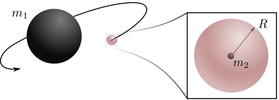
Figure 1: Our basic strategy: A region of radial extent $m_{2}\ll R\ll\mathcal{R}$ is excised from the computational domain ($\mathcal{R}$ being the characteristic lengthscale associated with the tidal field of the large mass $m_{1}$ at the location of the small mass $m_{2}$). An approximate analytical solution is used inside the excised region. The analytical and numerical solutions are dynamically matched at each step of the numerical evolution.

In this work we explore a new, synergistic approach to IMRI modelling, featuring a direct synthesis of black-hole perturbation and NR techniques. The central idea is simple, and illustrated in Fig. 1 as applied to a compact-object binary with masses $m_{1}\gg m_{2}$. An excision region is introduced around the small object, of radial extent $R$ chosen such that $m_{2}\ll R\ll\mathcal{R}$, where $\cal R$ is the characteristic lengthscale associated with the tidal field of $m_{1}$ at the location of $m_{2}$ (such that $\mathcal{R}\sim m_{1}$ near the end of the inspiral). Inside this region—a “worldtube” in spacetime—an approximate analytical solution is prescribed for the spacetime metric, arising from the perturbation theory of compact objects in a tidal environment. An NR simulation is set up for the binary, in which the worldtube’s interior is excised from the numerical domain, and replaced with the analytical solution. At each time step of the numerical evolution, the numerical solution (outside the tube) and analytical solution (inside the tube) are matched across the tube’s boundary, in a process that fixes a priori unknown tidal coefficients in the analytical solution, as well as gauge degrees of freedom. The intended effect of this construction is to partially alleviate the scale disparity that thwarts the efficiency of the numerical evolution at small $q$. An outline of such a strategy was first (to our knowledge) put forward by B. Schutz in a conference talk a few years ago [24].

To begin thinking about how such a strategy may work in practice, we restrict attention to the simplest scenario, where the smaller object is a black hole. The appropriate analytical solution inside the worldtube is then that of a tidally perturbed Kerr black hole, where the tidal perturbation arises from the presence of the larger body. Such geometries are examples of a broader class of spacetimes studied extensively in recent literature [25, 26, 27, 28, 29, 30, 31, 32, 33], where the tidal response of a compact object to an external perturbative tidal field is derived analytically order by order in $s/\mathcal{R}$—the ratio of distance $s$ from the smaller object and the characteristic lengthscale $\mathcal{R}$ of the tidal field—under the assumption $s\ll\mathcal{R}$. For a nonrotating black hole, the perturbed metric has so far been constructed through order $(s/\mathcal{R})^{4}$ [28]. For our excision method we would need the perturbed metric near the worldtube’s boundary, where it takes the form of an expansion in $R/\mathcal{R}\ll 1$.

Since the analytically prescribed metric on the worldtube’s boundary is only an approximation, the spacetime constructed in the numerical simulation is also approximate, even if numerical error could be reduced to zero. If our analytical solution is correct only up to $\mathcal{O}\left((R/\mathcal{R})^{n}\right)$—what we later call an “$n$th-order model”—then, in general, an error of $\mathcal{O}\left((R/\mathcal{R})^{n+1}\right)$ is fed from the tube’s boundary to the numerical solution, and propagates to the bulk of the numerical domain. One could then only hope to construct the binary’s spacetime up to an error of $\mathcal{O}\left((R/\mathcal{R})^{n+1}\right)$, even in the continuum limit. This worldtube error can be reduced either by increasing the order $n$ of the analytical model, or by decreasing the tube’s radius $R$. Of course, decreasing $R$ restores the original scale disparity and thus diminishes the gain from the introduction of a tube. There is hence a fundamental trade-off in our method between precision and computational cost, with $R$ serving as a control parameter. At the end of this introduction we give a rough estimation of the potential computational savings for an “optimal” choice of $R$.

Our primary purpose in this initial study is to develop and test a matching methodology for the field across the worldtube’s boundary. For that purpose we employ a linear scalar-field toy model, in which the small black hole is replaced with a pointlike scalar charge, and the large object is a Schwarzschild black hole. Instead of tackling the full Einstein’s equations, we thus solve the massless linear Klein-Gordon equation for a scalar field on a fixed Schwarzschild background. Furthermore, we decompose the field equation into multipole modes on the Schwarzschild geometry, and solve for each mode of the field individually as an evolution problem in 1+1 dimensions (radius+time). Our worldtube is then a 2-dimensional “strip” confined between two parallel timelike curves (cf. Fig. 3 below). As a final simplification, we set the scalar charge to move on a fixed circular geodesic orbit around the large black hole (ignoring radiation reaction), meaning we can fix our worldtube in advance of the evolution, and it has a simple geometry. All of these simplifications take us very far, of course, from the actual physical problem in question. However, our toy problem retains enough relevant features to make it useful as a development platform for worldtube matching procedures.

We develop and explore two such procedures. The first is based on matching the analytical and numerical solutions in an open “buffer” region around the tube’s boundaries. At each step of the time evolution, the matching determines a set of unknown coefficients in the analytical solution. Once the analytical solution has been fixed inside the tube, the evolution can proceed to the next time step. This approach is close in spirit to the standard method of matched asymptotic expansions, which underlies most of the literature on tidally perturbed black hole spacetimes (as well as GSF theory). But whereas in standard matched expansions one matches together two asymptotic expansions, here one matches an asymptotic expansion (the approximate analytical solution in the tube) to an “exact” numerical solution. The second matching approach we explore is conceptually different, reminiscent more of the standard treatment of interfaces between media in hyperbolic systems using a junction condition. In this approach we regard the worltube boundary as a strict interface, where boundary conditions are set for the numerical evolution outside the tube. These boundary conditions are obtained (at each time step) from solutions of a certain set of first-order ordinary differential equations (ODEs) along the boundary, formulated in a way that ensures well-posedness of the evolution scheme.

We formulate each of the two matching approaches quite independently of any implementation details; indeed, each approach can in principle be implemented using whichever one’s favorite numerical evolution method happens to be (finite difference or spectral, Cauchy or characteristic, etc.). Here, to illustrate the applicability of our two approaches and test their performance, we present two independent numerical implementations, one for each approach. For the first approach (matching in a buffer region) we present a finite-difference implementation in characteristic coordinates. For the second approach (matching on the boundary) we present a spectral implementation with Cauchy evolution. For each approach we demonstrate the stability and convergence of the numerical evolution, compare with analytical solutions where possible, and explore the dependence of the solutions on the worldtube radius $R$.

The paper is organised as follows. We begin in Sec. II by setting up our scalar-field toy model, with a point scalar charge on a circular geodesic sourcing a linear scalar field on a Schwarzschild background. We introduce a multipole-mode decomposition to reduce to problem to 1+1 dimensions, and (at the single-mode level) prescribe a suitable approximate analytical solution for the scalar field near the scalar charge, later to populate the interior of the worldtube around the charge.

Section III explains the general principles of our two matching approaches, in a language that is divorced from any implementation details. Our two particular numerical implementations—henceforth referred to as “scheme I” and “scheme II”—are described and explored in Secs. IV to VII. Section IV begins with a detailed description of our numerical method in scheme I, based on a finite-difference formula in null coordinates and characteristic evolution. Particular attention is paid to the development of matching architectures in a buffer region around the worldtube boundaries. In Sec. V we present various validation tests to demonstrate the stability and numerical convergence of our code and the correctness of the numerical results, and then focus on exploring the dependence of the numerical solution on $R$. Sections VI and VII do the same for scheme II, beginning with a detailed description of our spectral method and detailing the way boundary conditions are imposed on the worldtube. Section VIII contains a recap of our results, and a discussion of the next steps in the development of our approach to IMRI modelling.

First, however, let us conclude this introduction with a rough estimate of the runtime savings one might hope to achieve with our method.

I.1 Potential Runtime Savings

As already mentioned, the approximation error of the perturbative solution on the worldtube boundary is expected to be

$$\varepsilon_{\mathrm{WT}}~{}\sim\left(\frac{R}{\mathcal{R}}\right)^{n+1},$$ (1)

where $n$ is the order of the analytic solution, and $\cal R$ is the characteristic length scale associated with the tidal field of $m_{1}$ at $m_{2}$. Optimally, the approximation error $\varepsilon_{\mathrm{WT}}$ should be comparable to the error $\varepsilon_{\mathrm{NR}}$ of the NR simulation, i. e. $\varepsilon_{\mathrm{WT}}\sim\varepsilon_{\mathrm{NR}}$. This gives an “optimal” worldtube radius

$$R\sim\varepsilon_{\mathrm{NR}}^{1/(n+1)}\;\mathcal{R}.$$ (2)

For $n=4$ (as presently available for a tidally perturbed Schwarzschild black hole [26]) the dependence on $\varepsilon_{\mathrm{NR}}$ is quite weak. As an example, $\varepsilon_{\mathrm{NR}}=10^{-5}$ and $n=4$ yield $R\sim 0.1\mathcal{R}$. As a measure of $\cal R$ we may use the Kretschmann scalar $K=R_{\alpha\beta\gamma\delta}R^{\alpha\beta\gamma\delta}$ associated with the Schwarzschild field of $m_{1}$, with Riemann tensor $R_{\alpha\beta\gamma\delta}$. This gives $\mathcal{R}\sim K^{-1/4}\sim 0.4(D^{3}/m_{1})^{1/2}$, where $D$ is the separation between the two black holes. For example, near the end of the inspiral ($D\sim 6m_{1}$) we have $\mathcal{R}\sim 6m_{1}$, and an optimal choice of $R\sim 0.6m_{1}$.

The efficiency gain of the worldtube method arises from the weakened CFL condition: The smallest scale on the numerical grid with a worldtube is $\sim R$ (as long as the worldtube is smaller than the more massive BH), while the smallest scale for the traditional simulation is $\sim m_{2}$. Therefore, the CFL condition allows a time-step larger by a factor $\sim R/m_{2}$. Assuming a comparable computational cost per time-step between worldtube and traditional methods, the speed-up will be

$$\text{speedup}\sim\frac{R}{m_{2}}\sim\varepsilon_{\mathrm{NR}}^{1/(n+1)}\,\frac{\mathcal{R}}{m_{2}}=\varepsilon_{\mathrm{NR}}^{1/(n+1)}\frac{\mathcal{R}}{m_{1}}\;q^{-1}.$$ (3)

Equation (3) suggests a potential speed-up proportional to $q^{-1}\gg 1$, with the constant of proportionality depending on the target error $\varepsilon_{\mathrm{NR}}$, the order of the analytical approximation $n$ and the length scale $\cal R$, itself depending on the orbital radius $D$. For $D$ in the relevant strong-field range between $\sim 6m_{1}$ and $\sim 10m_{1}$, and with our sample values $n=4$ and $\varepsilon_{\mathrm{NR}}=10^{-5}$, the constant of proportionality is around unity. Therefore, for example, a speed-up by a factor 100 seems feasible for mass-ratio $1:100$. To phrase this differently, the computational cost of evolving for one orbit with the worldtube approach could be similar to evolving one orbit of a comparable-mass BBH with traditional NR methods at the same numerical error $\varepsilon_{\mathrm{NR}}$.

We caution that our estimate here is extremely crude. For one, the error scaling in Eq. (1) turns out not to hold in that precise form in our actual numerical implementations, as described below. Moreover, Eq. (3) assumes that time-stepping error is always subdominant, which may only hold for high-order time-stepping schemes like those employed by the SpEC code [11]. And even if the substantial speed-up of Eq. (3) can be realized, high-mass-ratio simulations will remain more challenging than comparable mass simulations, because the duration of the inspiral increases with more extreme mass-ratios. A tighter $\varepsilon_{\mathrm{NR}}$ might also be required at more extreme mass ratios, to resolve the smaller amplitude of the gravitational waves and to preserve phase accuracy over the longer inspiral.

II Scalar-field Toy Model

Our toy model replaces the smaller black hole with a pointlike test particle endowed with a scalar charge $e$. The particle is in a circular geodesic orbit around the larger object, taken to be a Schwarzschild black hole of mass $M$. The orbiting charge sources a linear scalar field $\Phi$, which satisfies the Klein-Gordon equation

$$g^{\alpha\beta}\nabla_{\alpha}\nabla_{\beta}\Phi(x)=-4\pi\rho(x)\,.$$ (4)

Here $\nabla_{\alpha}$ is the covariant derivative compatible with the background Schwarzschild metric $g_{\alpha\beta}$, and $\rho(x)$ is the scalar charge density, represented by the distribution

$$\rho(x)=e\int_{-\infty}^{\infty}\frac{\delta^{4}[x^{\mu}-x^{\mu}_{p}(\tau)]}{\sqrt{-g}}d\tau\,,$$ (5)

in which $x^{\mu}_{p}$ denotes the coordinates of the particle’s worldline, parametrised with proper time $\tau$, and $g$ is the determinant of $g_{\alpha\beta}$. In a Schwarzschild coordinate system attached to the background Schwarzschild geometry we have, for our circular orbit, $r_{p}:=x_{p}^{r}=\text{const}$, and, without loss of generality, we set $\theta_{p}:=x_{p}^{\theta}\equiv\pi/2$. The particle’s geodesic orbit then has a tangent four-velocity given (in Schwarzschild coordinates $t,r,\theta,\phi$) by

$$u^{\alpha}:=dx^{\alpha}_{p}/d\tau=\gamma\left(1,\,0,\,0,\,\Omega\right)\,,$$ (6)

where $\Omega:=(d\phi_{p}/d\tau)/(dt_{p}/d\tau)=(M/r_{p}^{3})^{1/2}$ is the orbital angular velocity with respect to time $t$, and $\gamma:=(1-3M/r_{p})^{-1/2}$ is a gravitational redshift factor. In terms of time $t$, the particle’s Schwarzschild coordinates are

$$x_{p}^{\alpha}=\left(t,r_{p},\frac{\pi}{2},\Omega t\right)\,,$$ (7)

where, again without loss of generality, we have set $\phi_{p}=0$ at $t=0$.

Our toy model makes a further simplification: rather than tackling the field equation (4) in the 3+1D spacetime, we separate it into spherical-harmonic multipole modes (taking advantage of the background’s spherical symmetry), and solve for each multipole of the field in 1+1D (time+radius). To achieve this, we write

$$\Phi=\frac{e}{r}\sum_{\ell=0}^{\infty}\sum_{m=-\ell}^{\ell}\Psi_{\ell m}(r,t)Y_{\ell m}(\theta,\phi)\,,$$ (8)

where $Y_{\ell m}(\theta,\phi)$ are standard spherical harmonics, defined on 2-spheres $r=\text{const}$ around the large black hole, and the factor $\frac{1}{r}$ is introduced for later convenience. We insert the expansion (8) into Eq. (4), and on the right-hand side of the latter we substitute the completeness relation $\delta(\theta-\theta_{p})\delta(\phi-\phi_{p})/\sin\theta=\sum_{\ell m}Y_{\ell m}(\theta,\phi)\bar{Y}_{\ell m}(\theta_{p},\phi_{p})$, where an overbar denotes complex conjugation. By virtue of the orthogonality of the $Y_{\ell m}$ functions, one immediately obtains a separate equation for each of the time-radial functions $\Psi_{\ell m}(r,t)$. The equation reads

$$\frac{\partial^{2}\Psi_{\ell m}}{\partial t^{2}}-\frac{\partial^{2}\Psi_{\ell m}}{\partial{r^{*}}^{2}}+V_{\ell}(r)\Psi_{\ell m}=\\ S_{\ell m}(t)\delta(r^{*}-r_{p}^{*})\,,$$ (9)

where

$$V_{\ell}(r)=\left(1-\frac{2M}{r}\right)\left(\frac{\ell(\ell+1)}{r^{2}}+\frac{2M}{r^{3}}\right),$$ (10)

and

$$S_{\ell m}(t)=\frac{4\pi}{\gamma r_{p}}\,\bar{Y}_{\ell m}\left(\frac{\pi}{2},\Omega t\right)\,.$$ (11)

Here we have introduced the tortoise radial coordinate $r^{*}=r+2M\ln[r/(2M)-1]$, with $r^{*}_{p}:=r^{*}(r_{p})$.

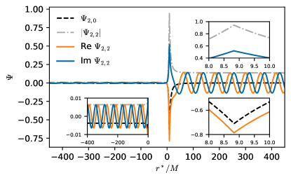
Figure 2: Illustration of the form of physical solutions to the modal scalar-field equation (9), with a source corresponding to a scalar charge on a circular geodesic orbit of radius $r_{p}=7M$ ($r_{p}^{*}\approx 8.83M$). Shown here are $\Psi_{22}$ and $\Psi_{20}$ as functions of the radial coordinate $r^{*}$ at some constant value of the time $t$. The field $\Psi_{22}$, which is radiative, is computed using the code presented in Subsec. IV.2; it displays scalar waves emanating from the particle down towards the event horizon ($r^{*}\to-\infty$) and out towards infinity ($r^{*}\to\infty$). The field $\Psi_{20}$, which is static, is given analytically in Eq. (12). For all values of $\ell,m$, the field is continuous at the location of the particle but has a finite jump discontinuity in its first radial derivative there.

Equation (9) is the basic field equation of our toy model, and in the rest of this work we apply our excision method to it in order to develop our strategy and test its performance. We aim to construct a solution of (9) subject to “physical” boundary conditions, namely that there is no radiation coming in from past null infinity or out of the past event horizon; we refer to that solution as the “physical” one. For benchmarking, it is useful to have at hand the actual physical solution of Eq. (9) (without a worldtube), and for that purpose we have developed a simple time-domain numerical code capable of accurately computing $\Phi_{\ell m}$ for given mode numbers $\ell,m$ and orbital radius $r_{p}$. The algorithm of our code, to be described in Sec. IV.2, is based on characteristic evolution with a second-order-convergent finite-difference formula, with the $\delta$-function source term incorporated by way of imposing suitable jump conditions along the particle’s worldline (see Sec. IV.2 for details). The typical form of the solution is illustrated in Fig. 2, showing a $t=\mathrm{constant}$ snapshot of the field $\Psi_{22}$. Notable features of the solution are (i) scalar-field waves (of frequency $m\Omega$) that emanate from the particle and show in the outer “wave zone”, $r^{*}\gg M$; (ii) scalar-field waves (again of frequency $m\Omega$ but typically of a lower amplitude) going into the black hole, visible at $r^{*}\ll-M$; and (iii) the cusp in the scalar field at the particle’s location, where $\Psi_{\ell m}$ is continuous but has a finite jump in its first radial derivative. Similar features characterise the solution for other $\ell$ and $m\neq 0$ modes.

For $m=0$ (axially symmetric) modes of the scalar-field perturbation, the source $S_{\ell m}$ becomes time-independent, and the physical solution is static. The field equation (9) then reduces to an ordinary differential equation, and admits simple analytical solutions. Such solutions are particularly useful for benchmarking purposes, and they will serve us well in that capacity later in our analysis. For a “physical” $m=0$ field we look for a static solution of Eq. (9) for which the modal Klein-Gordon field $\Phi_{\ell 0}(r):=\Psi_{\ell 0}(r)/r$ is bounded on the event horizon and falls off at infinity. It is not hard to see that these conditions define a unique solution for each $\ell$. The solution is given by

$$\begin{split}\Psi_{\ell 0}(r)=\frac{rr_{p}}{M}S_{\ell 0}\Big{(}&Q_{\ell}(z_{p})P_{\ell}(z)\Theta(r_{p}-r)\\ &+Q_{\ell}(z)P_{\ell}(z_{p})\Theta(r-r_{p})\Big{)}\,,\end{split}$$ (12)

where $P_{\ell}$ and $Q_{\ell}$ are Legendre functions of the first and second kind, respectively, with the arguments $z:=r/M-1$ and $z_{p}:=r_{p}/M-1$, and $\Theta(\cdot)$ is the Heaviside step function. An example of such a static solution, with $\ell=2$, is also shown in Fig. 2. The static modes, too, are continuous at the location of particle, and display a finite jump discontinuity in the first radial derivative there.

II.1 Local Approximate Solution

In our toy model we replace the actual solution in a worldtube surrounding the particle’s worldline with an analytical approximation $\Psi^{A}_{\ell m}$. The analytical solution consists of two terms: a “puncture” field $\Psi^{\mathcal{P}}_{\ell m}$, which captures the local irregularity in (i. e., discontinuous derivatives of) the field at the particle, and a “regular” field $\Psi^{\mathcal{R}}_{\ell m}$, which accounts for the remaining, smooth part of the local field. Both these terms are expressed as a power series in the distance to the worldline, truncated at a certain order (to be referred to as “the order” of the analytical model). The expansion coefficients of $\Psi^{\mathcal{P}}_{\ell m}$ can be determined analytically from the field equation (9) using a local asymptotic analysis, as we explain below, and are fixed in advance in our model. The expansion coefficients of $\Psi^{\mathcal{R}}_{\ell m}$, on the other hand, can only be determined by matching to the external field outside the worldtube; these coefficients remain a priori unknown, and they are to be determined dynamically during the numerical evolution as described in later sections. In the rest of this section we describe the construction of a suitable local analytical model $\Psi^{A}_{\ell m}$ for the scaler field. Preliminary considerations regarding the construction of such a model in the 3+1D gravity problem of our ultimate interest are discussed in Sec. VIII.

We begin with the construction of a suitable puncture field $\Psi^{\mathcal{P}}_{\ell m}$. Recalling our observation that the physical solution is continuous but has a finite jump discontinuity in its first radial derivative at the particle, we introduce the ansatz

$$\Psi^{\mathcal{P}}_{\ell m}(r,t)=\lvert\Delta r\rvert\sum_{j=1}^{n}a_{j\ell m}(\Delta r)^{j-1}S_{\ell m}(t)\,,$$ (13)

where $\Delta r:=r-r_{p}$. Our choice of time dependence here makes sense, because the source function $S_{\ell m}(t)$ depends on $t$ harmonically, via the factor $e^{-im\Omega t}$ implicit in $\bar{Y}_{\ell m}\left(\frac{\pi}{2},\Omega t\right)$ in Eq. (11), and the retarded solution inherits this harmonic time dependence. We terminate the expansion at order $(\Delta r)^{n}$ for some $n\geq 1$, referring to the resulting field as an “$n$th-order puncture”, denoted $\Psi_{\ell m}^{\mathcal{P}(n)}$.

The constant coefficients $a_{j\ell m}$ in Eq. (13) are determined by substituting (13) in the field equation (9), re-expanding in powers of $\Delta r$, and then demanding that the resulting equation is satisfied at the particle as a distributional equality. This produces a hierarchy of algebraic equations for $a_{j\ell m}$, which we can solve recursively order by order in $\Delta r$. More specifically, once (13) is substituted in (9), the requirement that the delta-function terms balance in the equation immediately determines $a_{1\ell m}$. Then, the requirement that the remaining discontinuity vanishes at $\mathcal{O}(\Delta r^{0})$ determines $a_{2\ell m}$ in terms of $a_{1\ell m}$, the requirement that it vanishes at $\mathcal{O}(\Delta r^{1})$ determines $a_{3\ell m}$ in terms of $a_{1\ell m}$ and $a_{2\ell m}$, and so on. For the first five coefficients one obtains, in this fashion,

$$a_{1\ell m} =-\frac{1}{2f_{p}}\,,$$ (14a)

$$a_{2\ell m} =\frac{M}{2f_{p}^{2}r_{p}^{2}}\,,$$ (14b)

$$a_{3\ell m} =\frac{r_{p}^{4}m^{2}\Omega^{2}-\lambda r_{p}^{2}f_{p}-2M(3r_{p}-2M)}{12f_{p}^{3}r_{p}^{4}}\,,$$ (14c)

$$a_{4\ell m} =\frac{\lambda r_{p}^{3}f_{p}-3Mr_{p}^{4}m^{2}\Omega^{2}+2M(3r_{p}^{2}-4Mr_{p}+2M^{2})}{12f_{p}^{4}r_{p}^{6}},$$ (14d)

$$a_{5\ell m} =\frac{1}{240f_{p}^{5}r_{p}^{8}}\Big{[}2r_{p}^{4}m^{2}\Omega^{2}\left(\lambda r_{p}^{2}f_{p}+2M(11r_{p}+13M)\right)$$

$$\quad-r_{p}^{8}m^{4}\Omega^{4}-2\lambda r_{p}^{2}f_{p}(9r_{p}^{2}+2Mr_{p}-4M^{2})$$

$$\quad-24M(5r_{p}^{3}-10Mr_{p}^{2}+10M^{2}r_{p}-4M^{3})$$

$$\quad-\lambda^{2}r_{p}^{4}f_{p}^{2}\Big{]}\,,$$ (14e)

where $f_{p}:=f(r_{p})=1-2M/r_{p}$ and $\lambda:=\ell(\ell+1)$. With this, we have all that we need to construct puncture fields through fifth order.

Next, consider the remaining piece of the local field, $\Psi_{\ell m}^{\mathcal{R}(n)}$, which we now define as the difference $\Psi_{\ell m}-\Psi_{\ell m}^{\mathcal{P}(n)}$ between the full physical field and the $n$th-order puncture field, expanded in $\Delta r$, with the expansion truncated at $\mathcal{O}(\Delta r^{n})$. Since, by construction, $\Psi_{\ell m}^{\mathcal{P}(n)}$ has the same singular structure as $\Psi_{\ell m}$ through $\mathcal{O}(\Delta r^{n})$, the so-defined field $\Psi_{\ell m}^{\mathcal{R}(n)}$ is smooth, and takes the form of a polynomial:

$$\Psi_{\ell m}^{\mathcal{R}(n)}(t,r)=\sum_{j=0}^{n}\psi^{\mathcal{R}}_{j}(t)(\Delta r)^{j}\,.$$ (15)

The $n+1$ coefficients $\psi^{\mathcal{R}}_{k}(t)$ (their $\ell,m$ indices suppressed for brevity) are a priori unknown; they are to be determined by matching to the numerical field outside the worldtube at each time step in the numerical evolution, as we describe in the next section.

Our full $n$th-order analytical approximate field inside the worldtube is given by

$$\Psi_{\ell m}^{A(n)}(t,r;\psi^{\mathcal{R}}_{k})=\Psi_{\ell m}^{\mathcal{P}(n)}(t,r)+\Psi_{\ell m}^{\mathcal{R}(n)}(t,r;\psi^{\mathcal{R}}_{k})\,,$$ (16)

where our notation reminds the reader that $\Psi_{\ell m}^{A(n)}$ inherits from $\Psi_{\ell m}^{\mathcal{R}(n)}$ a parametric dependence on the $n+1$ time-dependent coefficients $\psi^{\mathcal{R}}_{k}:=\{\psi^{\mathcal{R}}_{0}(t),\ldots,\psi^{\mathcal{R}}_{n}(t)\}$. We use the field $\Psi_{\ell m}^{A(n)}$ to populate the interior of the excision worldtube in our numerical simulations, with $\psi^{\mathcal{R}}_{k}$ determined by matching at each time step. The “approximate” nature of $\Psi_{\ell m}^{A(n)}$ comes from the finite truncation of the expansion in $\Delta r$ at order $n$. Note that, due to the finite truncation, our definition of $\Psi_{\ell m}^{A(n)}$ is attached to our particular choice of a distance expansion parameter: using e. g. $\Delta r^{*}$ instead of $\Delta r$ would yield a slightly different (but equally valid) analytic approximation. Note also that $\Psi_{\ell m}^{A(n)}$ cannot be “made exact” (even in principle) with a fine-tuned choice of the parameters $\psi^{\mathcal{R}}_{k}$, since these parameters control only the smooth piece of the field and cannot correct the error in the non-smooth piece caused by the finite truncation of $\Psi_{\ell m}^{\mathcal{P}(n)}$. The error in $\Psi_{\ell m}^{A(n)}$ is inherent, and can only be controlled by varying the model order $n$ (or the worldtube radius).

This concludes the formulation of our 1+1D scalar-field toy model. In the next section we formulate two (alternative) matching strategies for the field in and outside of the worldtube, and in later sections we use our toy model to test the implementation of each of these strategies. In the rest of the paper the $(n)$ superscript and $\ell m$ indices are mostly suppressed, for brevity.

III Two matching approaches

Using our toy model, we now develop our two matching approaches: one based on matching the numerical field to the analytical approximation $\Psi_{\ell m}^{A}$ in an open region around the particle, and another based on junction conditions imposed on the surface of the excision region. In this section we describe the principles behind each approach, keeping the descriptions independent of any particular choice of discretization.

III.1 First approach: matching in a buffer region

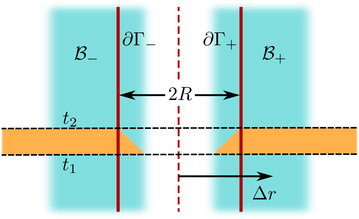
Figure 3: Spacetime diagram (in $t,r$ coordinates) illustrating the various regions involved in our first matching approach. The vertical dashed line indicates the particle’s worldline at constant orbital radius. The disjoint shaded regions $\mathcal{B}_{\pm}$ make up the buffer region $\mathcal{B}=\mathcal{B}_{-}\cup\mathcal{B}_{+}$ where the matching occurs. The excision region $\Gamma$ has a disjoint boundary $\partial\Gamma=\partial\Gamma_{+}\cup\partial\Gamma_{-}$ that lies within $\mathcal{B}$. We carry out the matching by expanding the numerical field $\Psi^{N}$ in powers of $\Delta r$ and equating the coefficients in the expansion to the coefficients in $\Psi^{A}$. The orange shaded region shows the domain of dependence of the field outside $\Gamma$ at time $t_{2}$, given data at time $t_{1}$.

Our first approach is inspired by the method of matched asymptotic expansions. Let us recall how that method is traditionally applied to the small-mass-ratio limit of the binary problem [34], with reference to Fig. 1. The binary is treated as a one-parameter system, using $m_{1}$ as an overall length scale and the small mass ratio $q=m_{2}/m_{1}$ as a small parameter (in this treatment, the length $\mathcal{R}$ utilized in the introduction is replaced with $m_{1}$ rather than being treated as an independent scale). In the bulk of the binary spacetime, one expands the metric in powers of $q$. Sufficiently near $m_{2}$, at distances $\sim m_{2}$, such an expansion breaks down because the gravity of $m_{2}$ dominates over that of $m_{1}$. One then constructs a complementary local approximation using an expansion in powers of $q$ while holding $s/m_{2}$ fixed, where $s$ is a suitable measure of spatial distance from the companion’s representative worldline. By holding $s/m_{2}$ fixed, this expansion zooms in on the region $s\sim m_{2}\ll m_{1}$, such that $s/m_{1}\sim q$. In a buffer region $m_{2}\ll s\ll m_{1}$, $s/m_{1}$ and $m_{2}/m_{1}$ are both small, and the exterior and interior approximations must agree. This requirement translates into a precise matching condition: if the local approximation inside the worldtube is re-expanded in powers of $q$ at fixed $s$ (no longer holding $s/m_{2}$ fixed), and the external solution is re-expanded in powers of $s/m_{1}$, then in both cases one arrives at a double series in $q$ and $s/m_{1}$, which should be a good approximation in the buffer region. The matching condition states that because they are expansions of the same metric, the two double expansions must agree term by term.

Now consider the translation of these notions into our toy problem. For simplicity we use $t$–$r$ coordinates in our description rather than the double-null coordinates we ultimately use in Scheme I. The setup in the $t$–$r$ plane is illustrated in Fig. 3. We define a buffer region $\mathcal{B}$, made up of disjoint regions $\mathcal{B}_{\pm}$, in which $\Delta r$ is small compared to $M$. We then define an excision region $\Gamma=[-R\leq\Delta r\leq R]$ around the particle’s orbital radius, with boundaries $\partial\Gamma_{\pm}$ lying in $\mathcal{B}_{\pm}$. We loosely imagine that outside of $\Gamma$, we solve for $\Psi$ using the homogeneous field equation, Eq. (9) with the right-hand side set to zero, and that inside, we use the analytical approximation $\Psi_{\ell m}^{A}$. For convenience, we label the numerically evolved field outside $\Gamma$ as $\Psi_{\ell m}^{N}$. However, following the dictates of matched expansions, we operate under the principle that in $\mathcal{B}$, $\Psi_{\ell m}^{N}$ and $\Psi_{\ell m}^{A}$ can be used interchangeably.

As in the method of matched expansions, to match the two fields we expand $\Psi^{N}$ to put it in the same form as $\Psi^{A}$ (we hereafter omit the indices $\ell m$ for brevity). In each of the regions $\mathcal{B}_{\pm}$, $\Psi^{N}$ can be approximated by a power series in $\Delta r$,

$$\Psi^{N\pm}(t,r)=\sum_{j=0}^{n}\psi^{\pm}_{j}(t)(\Delta r)^{j}+\mathcal{O}(\Delta r^{n+1})\,,$$ (17)

where $\Psi^{N\pm}$ denotes the restriction of $\Psi^{N}$ to $\mathcal{B}_{\pm}$. The coefficients $\psi^{\pm}_{j}$ can be found by projecting $\Psi^{N}$ onto the basis of functions $\{(\Delta r)^{0},\ldots,(\Delta r)^{n}\}$ using a suitable inner product

$$\langle x,y\rangle=\int_{\mathcal{B}^{\prime}}x(r)y(r)dr.$$ (18)

Here $\mathcal{B}^{\prime}$ is some open interval (with fixed $t$) in $\mathcal{B}$, or a collection of multiple such intervals; we consider the choice of integration domain below. Our matching condition is then that the coefficients in Eq. (17) are identical to the coefficients in $\Psi^{A}$:

$$\psi^{\pm}_{j}(t)=\psi^{\mathcal{R}}_{j}(t)+\psi^{\mathcal{P}\pm}_{j}(t)\,,$$ (19)

where $\psi^{\mathcal{P}\pm}$ are the puncture coefficients, which can be read off Eq. (13): $\psi^{\mathcal{P}\pm}_{j}(t)=\pm a_{j\ell m}S_{\ell m}(t)$.

To satisfy Eq. (19), we must ensure that $\psi^{\pm}_{j}$ satisfies the same jump conditions as $\psi^{\mathcal{P}\pm}_{j}$, meaning $\psi^{+}_{j}-\psi^{-}_{j}=\psi^{\mathcal{P}+}_{j}-\psi^{\mathcal{P}-}_{j}$. If we were to construct the approximations (17) separately in their respective regions $\mathcal{B}^{\pm}$, with no regard to the relationship between them, then these jump conditions would not be precisely satisfied. We enforce the correct jumps by demanding that the difference $\Psi^{N}-\Psi^{\mathcal{P}}$ is approximated by the smooth field $\Psi^{\mathcal{R}}$,

$$\Psi^{N}(t,r)-\Psi^{\mathcal{P}}(t,r)=\sum_{j=0}^{n}\psi^{\mathcal{R}}_{j}(t)(\Delta r)^{j}+\mathcal{O}(\Delta r^{n+1})\,.$$ (20)

This requires choosing the integration domain in Eq. (18) to have support in both ${\mathcal{B}}_{+}$ and ${\mathcal{B}}_{-}$. Taking the inner product of Eq. (20) with $(\Delta r)^{k}$ and discarding higher-order terms, we obtain a linear system for $\psi^{\mathcal{R}}_{j}$,

$$\sum_{j=0}^{n}A_{jk}\psi^{\mathcal{R}}_{j}(t)=b_{k}(t)~{}~{}~{}~{}~{}\text{for }k=0,\dots,n\,,$$ (21)

with $A_{jk}=\langle(\Delta r)^{j},(\Delta r)^{k}\rangle$ and $b_{k}=\langle\Psi^{N}-\Psi^{\mathcal{P}},(\Delta r)^{k}\rangle$. We note that the solution to Eq. (21) yields the $L^{2}$ best approximation of $\Psi^{N}-\Psi^{\mathcal{P}}$. Since this equation must hold for all $t$, it also implies an analogous equation for $\partial_{t}\psi^{\mathcal{R}}_{j}$, which is required for a Cauchy evolution.

To enforce the matching condition in a numerical evolution, we can use the following scheme:

1. Suppose that at time $t_{1}$, we have data for $\Psi^{N}$ and $\partial_{t}\Psi^{N}$ everywhere outside $\Gamma$.

2. Determine the approximate solution $\Psi^{A}(t_{1})$ and $\partial_{t}\Psi^{A}(t_{1})$ by solving Eq. (21) and the analogous equation for $\partial_{t}\psi^{\mathcal{R}}_{j}$. We then have $\Psi$ and $\partial_{t}\Psi$ for all $r$ at time $t_{1}$, given by the field values from Step 1 outside $\Gamma$ and by $\Psi^{A}$ and $\partial_{t}\Psi^{A}$ inside $\Gamma$.

3. Use the homogeneous equation, Eq. (9) with the right-hand side set to zero, together with the data at $t_{1}$ to obtain $\Psi^{N}$ at a later time $t_{2}$ everywhere outside $\Gamma$, as illustrated in Fig. 3. This requires data from inside $\Gamma$ at $t_{1}$, which is provided by $\Psi^{A}(t_{1},r)$ and $\partial_{t}\Psi^{A}(t_{1},r)$.

This can then be repeated indefinitely. Note that the time interval from one slice to the next is tied to the length scale of the buffer region. The evolution from $t_{k}$ to $t_{k+1}$ should only draw upon data for $\Psi^{A}$ in the buffer region, implying that the time intervals must be of order $R$ or shorter. In principle, this division of spacetime into time intervals need not be associated with one’s numerical discretisation, and the spacetime region between $t_{k}$ and $t_{k+1}$ can be spatially discretised in any convenient way.

Our description here refers to an evolution between slices of constant $t$, but it extends straightforwardly to any choice of slicing, including particularly the characteristic slicing we work with in Sec. IV. In general, the one-dimensional series approximation (17) is replaced by a two-dimensional series in powers of coordinate distances ($\Delta t$ and $\Delta r$ or appropriate null coordinates, for example) from a reference point on the worldline. The inner product (18) is then replaced by an integral over a two-dimensional region. We can also naturally extend the method to an evolution in $3+1$ dimensions by matching to a local approximation in a three- or four-dimensional region around the companion.

One additional aspect of this matching approach that should be noted is that it does not inherently impose any degree of differentiability across $\partial\Gamma_{\pm}$, except in the limit $n\to\infty$. This contrasts with our second matching approach, which we describe next.

III.2 Second approach: matching using junction conditions

Our second approach consists of matching the fields and its derivatives on the surface of the worldtube. As in the first approach, the regular part $\Psi^{\mathcal{R}}$ is a truncated Taylor series in $\Delta r^{*}$. However, here the coefficients are determined through a Hermite interpolation using values of the field and its derivatives up to a certain order $d$ on $\partial\Gamma_{-}$ and $\partial\Gamma_{+}$, i. e. we solve the system

$$\begin{split}\left.\partial_{r^{*}}^{k}\left(\Psi^{N}-\Psi^{\mathcal{P}}-\sum_{j=0}^{2d+1}\psi^{\mathcal{R}}_{j}(\Delta r^{*})^{j}\right)\right|_{\partial\Gamma_{\pm}}=0&\\ \text{for }k=0,\dots,d&\,,\end{split}$$ (22)

which is a system of $(2d+2)$ linear equations for the $(2d+2)$ coefficients $\psi^{\mathcal{R}}_{j}$. Unlike in the previous scheme, here we take the expansion order of the puncture field, $n_{\mathcal{P}}$, and that of the regular field, $n_{\mathcal{R}}=2d+1$, as independent. The overall convergence of the scheme with respect to $R$ is hence limited by $n_{\mathcal{P}}$ and $n_{\mathcal{R}}$. The same procedure is carried out for the time derivative of the regular part $\dot{\Psi}^{\mathcal{R}}$ and potentially further reduction variables. The Taylor expansions are then used to construct the boundary data that must be provided on the worldtube.

Boundary conditions can be interpreted and implemented as modifications to the right-hand sides of the bulk partial differential equations (PDEs), which we assume to be strongly hyperbolic, as it is the case for our wave equation toy model. The system remains well-posed if the boundary conditions retain strong hyperbolicity, which is the case when the coefficients of the series expansion are constructed from non-principal derivatives of $\Psi^{N}$ only. At first sight this severely limits the achievable expansion order, because we can use at most up to first derivatives of $\Psi^{N}$ and only field values of $\dot{\Psi}^{N}$. However, this limitation can be overcome by introducing an auxiliary system of ODEs evolving variables that represent the derivatives $\partial_{r^{*}}^{k}\Psi^{N}|_{\partial\Gamma_{\pm}}$ and $\partial_{r^{*}}^{k}\dot{\Psi}^{N}|_{\partial\Gamma_{\pm}}$ up to derivative order $d$. The ODEs must be formulated compatibly with the bulk PDEs, which can be done by taking derivatives of the bulk equations. The coefficients $\psi^{\mathcal{R}}_{j}$ are then computed using these auxiliary variables instead of data from the bulk PDEs. The auxiliary ODE system is solved simultaneously with the PDE system in a fashion not involving principal (or higher) derivatives of the PDE variables.

The boundary regular field derivatives $\partial_{r^{*}}^{k}\Psi^{\mathcal{R}}|_{\partial\Gamma_{\pm}}$ are related to the coefficients $\psi^{\mathcal{R}}_{j}$ through a simple matrix transform that follows from Eq. (22):

$$\left.\frac{\partial^{k}\Psi^{\mathcal{R}}}{\partial{r^{*}}^{k}}\right|_{\partial\Gamma_{\pm}}=\sum_{j=0}^{2d+1}\psi^{\mathcal{R}}_{j}\left.\frac{\partial^{k}(\Delta r^{*})^{j}}{\partial{r^{*}}^{k}}\right|_{\partial\Gamma_{\pm}}~{}~{}~{}\text{for }k=0,\dots,d\,.$$ (23)

Hence, for a linear system like the wave equation, this approach of using auxiliary ODEs is equivalent to evolving the regular part of the field inside the worldtube using a spectral method, similar to puncture schemes in self-force calculations, as is discussed in the next section. For nonlinear systems however this split into a regular part might not be possible and the scheme presented here could be a viable prototype when dealing with such systems. From the equivalence to a collocation-based spectral method it is possible to derive a numerically stable scheme to couple the bulk PDEs to the auxiliary system. This equivalence also explains how to control non-local effects that one might expect in an excision scheme. As long as the stability criteria of the equivalent spectral method are satisfied, this excision approach will satisfy them as well. These criteria entail satisfaction of a CFL-like inequality and using “energy preserving” boundary conditions. For a nonlinear field equation, this discretization using boundary derivatives will no longer be equivalent to a collocation-based method. However, both approaches converge to the same continuum limit and all stability criteria should still apply.

Our second matching approach will be developed in full in Sec. VI using a spectral method formulated on Cauchy slices, and its performance will be explored in Sec. VII.

III.3 Error estimates and connection to standard puncture methods

Our excision procedure is similar in some ways to the puncture schemes used in numerous self-force calculations [14, 15]. However, there is a crucial difference that we clarify (and motivate) here.

In a standard puncture scheme, one splits the exact field into two pieces, $\Psi=\tilde{\Psi}^{\mathcal{P}}+\tilde{\Psi}^{\mathcal{R}}$. Here $\tilde{\Psi}^{\mathcal{P}}$ captures the local singularity at the particle but is attenuated to zero outside some neighborhood of the particle. For example, it could be the field $\Psi^{\mathcal{P}}$ we work with in this paper but multiplied by a step function $\theta(R-|\Delta r|)$ that vanishes outside $\Gamma$. Unlike the field $\Psi^{\mathcal{R}}$ that we work with, $\tilde{\Psi}^{\mathcal{R}}$ is the exact difference $\tilde{\Psi}^{\mathcal{R}}:=\Psi-\tilde{\Psi}^{\mathcal{P}}$.

Using this split, one treats $\tilde{\Psi}^{\mathcal{R}}$ as the field variable, rearranging Eq. (9) to formulate a field equation with an effective source,

$$\Box\tilde{\Psi}^{\mathcal{R}}=S(t)\delta(r^{*}-r^{*}_{p})-\Box\tilde{\Psi}^{\mathcal{P}}:=S^{\rm eff}\,,$$ (24)

where for brevity we have defined $\Box:=\partial_{t}^{2}-\partial^{2}_{r^{*}}+V$ and continued to omit $\ell m$ labels. Equation (24) is solved over the entire domain, without excising a region around the particle, and with the same boundary conditions on $\tilde{\Psi}^{\mathcal{R}}$ as on $\Psi$. In such a scheme, there is no approximation: outside the support of $\tilde{\Psi}^{\mathcal{P}}$, the solution for $\tilde{\Psi}^{\mathcal{R}}$ is identical to $\Psi$; inside, one can add $\tilde{\Psi}^{\mathcal{P}}$ to likewise obtain the exact $\Psi$.

While this method is well suited to linear field equations, its applicability to the fully nonlinear Einstein equations is unclear. Due to nonlinearities, the metric of a tidally perturbed black hole is not a simple sum of singular and regular pieces, and one cannot simply move a piece of the metric to the right-hand side of the field equations. The excision methods we explore in this paper represent an alternative that should extend to the nonlinear problem. However, they do so at the cost of introducing an approximation: unlike a traditional puncture scheme, our methods do not yield the exact field $\Psi$.

First consider the error in our method inside $\Gamma$. In that region we use the approximation $\Psi^{A}$, which differs from $\Psi$ by an amount of order $(\Delta r)^{n+1}$ at best. This is a best-case estimate because it assumes that our matching methods enforce the exact values $\frac{1}{j!}\partial_{r}^{j}(\Psi-\Psi^{\mathcal{P}})\rvert_{r=r_{p}}$ for the coefficients $\psi^{\mathcal{R}}_{j}$ in Eq. (15). For simplicity, let us assume this best case.

Now consider the field outside $\Gamma$. More concretely, consider a bounded region $V$ with $\partial\Gamma$ as one of its boundaries; in a Cauchy evolution, the other boundaries might be an initial-data surface (outside $\Gamma$) and timelike boundaries far away, for example. Inside $V$, our field $\Psi^{N}$ satisfies the same homogeneous field equation as $\Psi$, $\Box\Psi^{N}=0$, but it inherits errors that propagate out from $\Gamma$. Those errors can be understood by writing $\Psi^{N}$ in a Kirchhoff integral form [34]. We introduce a retarded Green’s function satisfying

$$\Box G(\bm{x},\bm{x}^{\prime})=\Box^{\prime}G(\bm{x},\bm{x}^{\prime})=\delta^{2}(\bm{x},\bm{x}^{\prime})\,,$$ (25)

where $\bm{x}=(t,r^{*})$, $\Box^{\prime}:=\partial_{t^{\prime}}^{2}-\partial^{2}_{r^{\prime*}}+V(r^{\prime})$, and $\delta^{2}(\bm{x},\bm{x}^{\prime}):=\delta(t-t^{\prime})\delta(r^{*}-r^{\prime*})$. If we now take any point $\bm{x}\in V$, then the equations (25) and $\Box\Psi^{N}=0$ imply the identity

$$\Psi^{N}(\bm{x}^{\prime})\Box^{\prime}G(\bm{x},\bm{x}^{\prime})\\ -G(\bm{x},\bm{x}^{\prime})\Box^{\prime}\Psi^{N}(\bm{x}^{\prime})=\Psi^{N}(\bm{x}^{\prime})\delta^{2}(\bm{x},\bm{x}^{\prime})\,.$$ (26)

Integrating this equation over all $\bm{x}^{\prime}\in V$ and then using integration by parts, we obtain the Kirchhoff representation

$$\Psi^{N}(\bm{x}) =\int_{V}\left[\Psi^{N}(\bm{x}^{\prime})\Box^{\prime}G(\bm{x},\bm{x}^{\prime})\right.$$

$$\qquad\qquad\left.-G(\bm{x},\bm{x}^{\prime})\Box^{\prime}\Psi^{N}(\bm{x}^{\prime})\right]d^{2}x^{\prime}\,,$$

$$=\int_{\partial V}\left[\Psi^{N}(\bm{x}^{\prime})\partial_{n^{\prime}}G(\bm{x},\bm{x}^{\prime})\right.$$

$$\qquad\qquad\left.-G(\bm{x},\bm{x}^{\prime})\partial_{n^{\prime}}\Psi^{N}(\bm{x}^{\prime})\right]ds^{\prime}\,.$$ (27)

Here the coordinate area element in $V$ is $d^{2}x^{\prime}=dt^{\prime}dr^{\prime*}$. $\partial_{n^{\prime}}$ is the partial derivative normal to the boundary $\partial V$, and $ds^{\prime}$ is the coordinate line element on the boundary. For us the relevant portions of $\partial V$ are the worldtube boundaries $\partial\Gamma_{\pm}$, where $\partial_{n^{\prime}}=\mp\partial_{r^{\prime*}}$ and $ds^{\prime}=dt^{\prime}$.

From the Kirchhoff form, we see that $\Psi^{N}$ inherits two errors, respectively proportional to the errors in $\Psi^{N}\rvert_{\partial\Gamma}$ and $\partial_{r^{*}}\Psi^{N}\rvert_{\partial\Gamma}$. Suppose that $\Psi^{N}=\Psi^{A}+\mathcal{O}(|\Delta r|^{n+1})$ in an open neighbourhood of $\partial\Gamma$, as we seek to enforce in our first matching approach. Then $\Psi^{N}\rvert_{\partial\Gamma}$ has an error of order $R^{n+1}$, but $\partial_{r^{*}}\Psi^{N}\rvert_{\partial\Gamma}$ has an error of order $R^{n}$. The field $\Psi^{N}$ therefore differs from $\Psi$ by $\mathcal{O}(R^{n})$ throughout $V$. This represents a loss of one order relative to the $\mathcal{O}(R^{n+1})$ scaling that one might naively expect. Our numerical analysis in Sec. V confirms this $\mathcal{O}(R^{n})$ error estimate. However, our second matching approach more directly controls derivatives at $\partial\Gamma$, and in Sec. VII we find that in certain cases this second approach yields the more rapid, $\mathcal{O}(R^{n+1})$ convergence.

Analogous error estimates can be obtained for the 3+1D problem using a covariant Kirchhoff representation of the form (138) in Ref. [35]. A similar estimation might also be possible in fully nonlinear general relativity using Eq. (39) of that reference (reproduced from Ref. [36]).

IV Scheme I: Numerical Method

IV.1 Setup

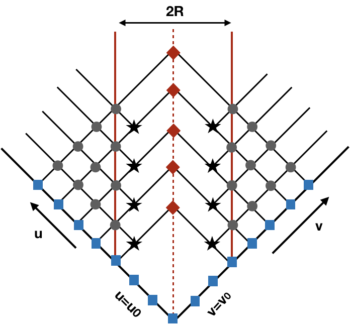
Figure 4: The 1+1D characteristic mesh used in Scheme I, with a fixed, uniform grid based on Eddington-Finkelstein coordinates $u,v$. The particle’s circular orbit is represented by the dashed (red) line running vertically down the center. The solid (red) vertical lines mark the boundaries of the excision worldtube. Outside the worldtube we evolve the field equation numerically along characteristic rays (as described in the text) using a finite-difference formula detailed in Sec. IV.2. The evolution starts from characteristic initial data set on the two initial rays $v=v_{0}$ and $u=u_{0}$ (blue square grid points) and proceeds to determine the data points in the bulk of spacetime outside the tube and on its boundaries (grey circle points). At each time step, a matching procedure, described in Sec. IV.3, is applied to determine the parameters of the approximate analytical solution on the remaining sections of the characteristic rays inside the tube, and in particular on the two “ghost” grid points (black, starred) needed at subsequent steps of the evolution.

In Scheme I we use a finite-difference method based on a uniform, fixed characteristic mesh in Eddington–Finkelstein coordinates

$$u=t-r^{*},\quad\quad v=t+r^{*}.$$ (28)

Figure 4 illustrates the basic setup. The numerical evolution starts from characteristic initial data specified on two initial rays $v=v_{0}$ and $u=u_{0}$ (blue, square grid points in the figure), chosen to intersect at the radius $r^{*}=r^{*}_{p}$ of the scalar charge’s circular orbit (dashed red line running vertically at the centre of the grid); that is, $v_{0}-u_{0}=2r_{p}^{*}$. An excision worldtube of width $\Delta r^{*}=2R$ is introduced around the orbit, with boundaries at $r^{*}=r^{*}_{p}\pm R$ (vertical red lines), chosen to intersect grid points. The numerical evolution proceeds along successive characteristic rays using a finite-difference formula to be described in Sec. IV.2 below. At each “time step”, we integrate first along a $u=\mathrm{const}$ ray starting at $v=v_{0}$ and progressing outwards up until tube’s left boundary, and then along the corresponding incoming ray $v=u+2r_{p}^{*}$ starting at $u=u_{0}$ and progressing inwards down to the tube’s right boundary. At each time step, a matching procedure then follows (described in Sec. IV.3 below), in which the value of the analytical model $\Psi^{A}$ is determined along the remaining sections of the two rays inside the tube. In particular, we assign analytical values to two ‘ghost’ grid points adjacent to the tube’s boundary in its interior (black starred points in the figure); these are needed for the subsequent time step of the numerical evolution.

Our characteristic mesh has a fixed (pre-set) stepping interval $h$ in both $u$ and $v$. The value of the field at a grid point with coordinates $(u,v)$ outside the tube (or on its boundary) is determined by our finite-difference formula based only on previously obtained values at the three grid points with coordinates ($u-h,v$), ($u,v-h$) and $(u-h,v-h)$. This, as we show in Sec. IV.2, suffices for obtaining a quartic $\mathcal{O}(h^{4})$ local convergence and a quadratic $\mathcal{O}(h^{2})$ global convergence.

The physical initial data for the numerical evolution are, of course, unknown to us except in the case of stationary, $m=0$ modes, where the entire solution is known analytically, Eq. (12). We thus resort to assigning fictitious initial data, and rely on dissipation of the resulting junk radiation over time. In post-processing we monitor the level of residual junk radiation, discard the early, junk-contaminated portion of the evolution, and retain only the remaining underlying “physical”, approximately stationary solution. In practice, we choose to set $\Psi=\Psi^{\mathcal{P}}$ on the portions of the rays $v=v_{0}$ and $u=u_{0}$ inside the worldtube, and attenuate smoothly to zero with a Gaussian across the tube’s boundary. The value of the field $\Psi$ on the two complete rays $v=v_{0}$ and $u=u_{0}$ suffices, in principle, to determine the solution anywhere in the domain of dependence $u>u_{0}$ and $v>v_{0}$.

IV.2 Finite-difference formula

We now describe the algorithm used to integrate the wave equation numerically outside the excision region. Our method is a standard one, used extensively in self-force literature, legacy of early work by Lousto and Price [37]. Since we evolve numerically only in the vacuum region outside the excision tube, it suffices to consider the scalar field equation (9) in vacuum. In terms of the $u,v$ coordinates it reads

$$\partial_{u}\partial_{v}\Psi+\frac{1}{4}V(r)\Psi=0\,,$$ (29)

where hereafter $\partial_{u}$ is taken with fixed $v$ and $\partial_{v}$ is taken with fixed $u$. Our goal is to write a finite-difference version of this equation on the characteristic grid described above.

To this end, consider a generic vacuum grid point with coordinates $(u,v)$, and assume the field has been computed in previous steps at all grid points within the past “light cone” of $(u,v)$ (to the future of the initial surfaces). Consider the grid ‘cell’ with vertices $(u,v)$, ($u-h,v$), ($u,v-h$) and $(u-h,v-h)$, where, recall, $h$ is our fixed step size in both $u$ and $v$. To obtain our finite-difference formula, it is convenient to consider the formal integral of both sides of Eq. (29) over the area of the grid cell. For the principal part of the equation we obtain

$$\begin{split}\iint_{\mathrm{cell}}\partial_{uv}\Psi dudv&=\Psi(u,v)-\Psi(u,v-h)\\ &-\Psi(u-h,v)+\Psi(u-h,v-h)\,,\end{split}$$ (30)

which is exact, and does not incur any finite-differencing error. For the potential term in Eq. (29) we obtain

$$\frac{1}{4}\iint_{\mathrm{cell}}V(r)\Psi dudv= \frac{h^{2}}{8}V(r_{c})\Big{[}\Psi(u,v-h)+\Psi(u-h,v)\Big{]}$$

$$+\mathcal{O}(h^{4}),$$ (31)

where $V(r_{c})$ is the value of the potential at the centre of cell, i. e. at $r^{*}_{c}=(v-u-h)/2$. Since the cell integral of the right-hand side of Eq. (29) is zero, combining the above results gives

$$\Psi(u,v)= \big{[}\Psi(u,v-h)+\Psi(u-h,v)\big{]}\bigg{[}1-\frac{h^{2}}{8}V(r_{c})\bigg{]}$$

$$-\Psi_{1}(u-h,v-h)+\mathcal{O}(h^{4}).$$ (32)

This simple finite-difference formula has a local error of $\mathcal{O}(h^{4})$ at each vacuum grid point. Since the total number of vacuum grid points scales as $1/h^{2}$ (for fixed physical grid dimensions), we expect the global cumulative error to scale like $h^{2}$.

We note that the above, quadratically convergent scheme requires only three input data points to determine the field value at each vacuum point. These three data points are always available from previous steps of the characteristic evolution. To calculate points that are on the tube’s boundary, an input data point is required from inside the tube. For this internal point we use the value of the approximate analytical field $\Psi^{A}$, which will have been fitted for in the previous time step of the evolution, using the procedure described in Sec. IV.3 below.

IV.2.1 Test evolution with a point particle and no excision

For test and benchmarking, we have also developed a version of our code that solves the full inhomogeneous field equation (9) as it is, without an excision. In this case the vacuum regions extend to the exposed scalar charge, and we must modify our finite-difference scheme to account for the presence of the sourcing particle. Our vacuum formula (32) still applies at all grid points, except points sitting directly on the particle’s worldline at $r^{*}=r_{p}^{*}$, for which we need a modified formula.

In $u,v$ coordinates, the inhomoheneous field equation (9) becomes

$$\partial_{u}\partial_{v}\Psi+\frac{1}{4}V(r)\Psi=\frac{1}{4}S(t)\delta(r^{*}-r^{*}_{p})\,.$$ (33)

Consider a generic worldline grid point at $(u,v)$, such that $v-u=2r_{p}^{*}$. To write down a finite-difference expression for the field at $(u,v)$, we again integrate both sides of the equation over the cell with $(u,v)$ at its upper vertex. Recalling that (in the continuous limit) solutions are continuous (albeit generally not differentiable) on the particle’s worldline, we find that Eq. (30) for the principal part still holds exactly, even for cells crossed by the particle. Equation (IV.2) for the potential term also holds, but the error term is expected to be of $\mathcal{O}(h^{3})$ in general, due to the discontinuous derivative. This, however, would suffice for our purpose, since the number of worldline points scale only as $1/h$, and so a local error of $\mathcal{O}(h^{3})$ should lead to an cumulative global error of only $\mathcal{O}(h^{2})$, consistent with our quadratic-convergence standard.

It remains only to evaluate the cell integral of the right-hand side of (33). To this end, we recall the form of the source function $S(t)$, given in Eq. (11); it depends on $t$ only through the factor $\bar{Y}_{\ell m}\left(\frac{\pi}{2},\Omega t\right)$, which itself depends on $t$ only through the factor $e^{-im\Omega t}$. It is therefore convenient here to write

$$S(t)=A_{\ell m}e^{-im\Omega t},$$ (34)

where, we obtain,

$$A_{\ell m}=\frac{(-1)^{\frac{\ell+m}{2}}}{\gamma r_{p}}\bigg{[}\frac{4\pi(2\ell+1)(\ell+m-1)!!(\ell-m-1)!!}{(\ell+m)!!(\ell-m)!!}\bigg{]}^{1/2}$$ (35)

when $\ell+m$ is even, or $A_{\ell m}=0$ when $\ell+m$ is odd. The cell integral over the source can now be readily evaluated in exact form, giving

$$\begin{split}Z:&=\frac{1}{4}\iint_{\mathrm{cell}}S(t)\delta(r^{*}-r^{*}_{p})dudv\\ &=\frac{1}{2}hA_{\ell m}\,\operatorname{sinc}\left(\frac{m\Omega h}{2}\right)e^{-im\Omega t_{c}},\end{split}$$ (36)

where $\operatorname{sinc}x:=(\sin x)/x$ and $t_{c}$ is the value of $t$ at the center of the cell in question, i. e. $t_{c}=(v+u-h)/2$.

Collecting the above results, we arrive at the following finite-difference formula, applicable at grid points traversed by the particle:

$$\Psi(u,v)= \big{[}\Psi(u,v-h)+\Psi(u-h,v)\big{]}\bigg{[}1-\frac{h^{2}}{8}V(r_{c})\bigg{]}$$

$$-\Psi_{1}(u-h,v-h)+Z+\mathcal{O}(h^{3}).$$ (37)

For our test evolution with a point particle, we use the vacuum formula (32) at all grid points except those on the particle’s worldline, for which we use (37). With this, we expect (and observe) a global quadratic convergence with $h$.

IV.3 Matching procedure

Scheme I employs the matching approach described in Sec. III.1, i. e. matching in a buffer region. In practice, the implementation is a discretised version of the approach, and the integral in Eq. (18) reduces to a summation over discrete data points. With $i$ labelling the discrete data points, Eq. (21) becomes

$$\sum_{j=0}^{n}A_{jk}\psi^{\mathcal{R}}_{j}(t)h=b_{k}(t)h~{}~{}~{}~{}~{}\text{for }k=0,\dots,n\,,$$ (38)

with $A_{jk}=\sum_{i=1}^{d}\Delta r_{i}^{j}\Delta r_{i}^{k}$ and $b_{k}=\sum_{i=1}^{d}(\Psi^{N}_{i}-\Psi^{\mathcal{P}}_{i})\Delta r_{i}^{k}$. The discretisation factor $h$, appears on both sides of Eq. (38) and cancels. The number $d$ of data points must be taken to be greater than or equal to the number of unknown coefficients $\psi^{\mathcal{R}}_{j}$, and the solution to Eq. (38) then yields the least-squares polynomial regression of $\Psi^{N}_{i}-\Psi^{\mathcal{P}}_{i}$. It should be noted that alternative matching methods could be used. However, we adopt the standard least-squares polynomial regression for simplicity at this trial stage.

The above description assumes (for simplicity) a Cauchy-type evolution, and it needs to be adapted for use in our characteristic evolution setup. In the Cauchy evolution case, the regular field component of the analytical solution is expanded in powers of $\Delta r$ about the point where the current Cauchy slice intersects the particle’s worldline (at the center of the tube; refer again to Fig. 3). In our characteristic implementation, we instead choose to expand $\Psi^{\mathcal{R}}(u,v)$ as a double Taylor series in $\Delta u:=u-u_{p}$ and $\Delta v:=v-v_{p}$ about the point of intersection of the two current null slices $(u_{p},v_{p})$, which in our setup is a point along the particle’s worldline at the center of the tube (refer again to Fig. 4). The expansion takes the form

$$\Psi^{\mathcal{R}}(u,v)=\sum_{i=0}^{n}\sum_{j=0}^{n-i}\psi^{\mathcal{R}}_{ij}{\Delta u}^{i}{\Delta v}^{j},$$ (39)

where $n$ is the puncture order, and the coefficients $\psi^{\mathcal{R}}_{ij}$ are a priori unknown constant coefficients at each time step. There are $N=(n+1)(n+2)/2$ such coefficients. The matching conditions in Eq. (38) are then replaced with a suitable two-dimensional version, with solutions that are the least-squares 2D polynomial regression model of $\Psi^{N}_{i}-\Psi^{\mathcal{P}}_{i}$ over a 2D array of data points in the $u,v$ plane. For this to work, one must take $d\geq N$, i. e. the number of data points must be greater than or equal to the number of coefficients $\psi^{\mathcal{R}}_{ij}$.

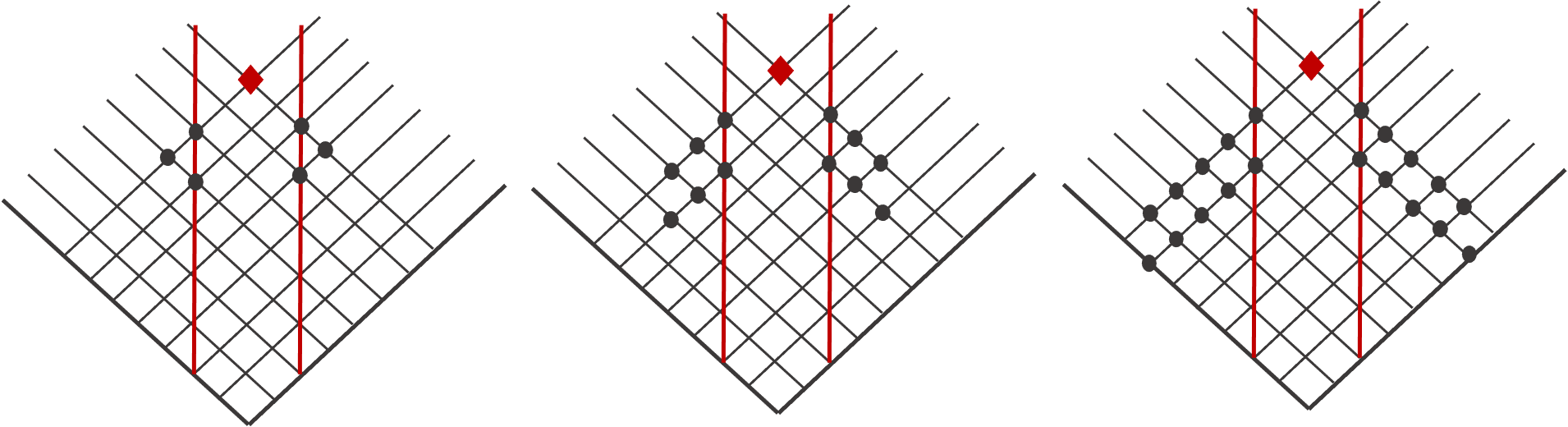
Figure 5: Data used to fit for the unknown parameters $\psi^{\mathcal{R}}_{ij}$ in the linear, quadratic and cubic-order approximate analytical models ($n=1,2$ and $3$, left to right respectively). Red vertical lines mark the worldtube’s boundaries, and the red diamond is the reference point about which the regular field is expanded in a double Taylor series. Black circles represent the numerically determined field data points used to the fit the parameters $\psi^{\mathcal{R}}_{ij}$ of the analytical model inside the tube, using the procedure described in the text.

In our particular implementation we choose to take $d=2N$, i. e. twice as many data points as unknown coefficients. This choice appeared to provide a good balance in the tradeoff between accuracy and runtime. Since, with this choice, the number of data points is always even, it allows us to distribute them evenly and symmetrically either side of the worldtube. Our choice of data points for the matching, for model orders $n=1,2$ and $3$, is shown in Fig. 5. In all cases, we draw our matching points from the current two null rays and from the two null rays in the preceding time step (it is necessary to use data from more than a single time step in order to fit for mix-derivative coefficients like $\psi^{\mathcal{R}}_{11}$).

With these choices, the matching procedure is as follows. As described already, at each time step we evolve the initial data using successive applications of our finite-difference formula along the corresponding two null rays $u=\mathrm{const}$ and $v=\mathrm{const}$ (such that $v-u=2r_{p}^{*}$) running from the initial null surfaces to the boundaries of the tube. Once this step is completed, we record the $d$ numerical data points $\Psi^{N}_{i}$ shown in Fig. 5, all of which are known to us from the current or previous steps of the numerical evolution, and then construct the $d$ values $\Psi^{N}_{i}-\Psi^{\mathcal{P}}_{i}$ by subtracting the analytically known puncture values at the corresponding grid points. To these $d$ values we now match the $n$th-order 2D polynomial given in Eq. (39) using a least-square minimisation procedure to obtain the coefficients $\psi^{\mathcal{R}}_{ij}$. This, in turn, determines the regular field $\Psi^{\mathcal{R}}$, and thus also the complete analytical approximation $\Psi^{A}=\Psi^{\mathcal{R}}+\Psi^{\mathcal{P}}$ inside the worldtube, in the vicinity of the current characteristic rays. We record the values of $\Psi^{A}$ at the two “ghost” grid points inside the tube adjacent to the boundaries on the current ray (starred points in Fig. 4); these two values will be required when calculating the numerical field on the boundary in the next time step. This concludes the computation for the current time step, and we can now step forward in (advance/retarded) time and repeat.

A few comments are in order. First, it may be noticed that in the first few time steps of the evolution there may not be available sufficiently many data points to fit all of the $N$ model parameters. In such cases we simply set to zero the values of the “missing” data points. This does not cause a problem, because the early evolution is in any case dominated by non-physical junk radiation; all this does is modify the profile of the initial junk.

Second, we note that in our procedure we choose not to impose that $\Psi^{A}$ satisfies the field equation in the tube; if we did, some of the coefficients $\psi^{\mathcal{R}}_{ij}$ would become mutually dependent. For example, in the quadratic model with $n=2$, imposing the field equation would determine the coefficient $\psi^{\mathcal{R}}_{11}$ in terms $\psi^{\mathcal{R}}_{00}$, $\psi^{\mathcal{R}}_{01}$ and $\psi^{\mathcal{R}}_{10}$. Such an alternative approach is possible, but we find that it does not leads to any marked improvement in either accuracy or speed. For simplicity, we thus opt to treat all $N$ coefficients $\psi^{\mathcal{R}}_{ij}$ as independent for the purpose of matching.

Finally, we comment on the degree of differentiability of our solution on the tube’s boundary. As already mentioned, since we are not explicitly imposing continuity of the field or its derivatives at the tube’s boundary, there is no reason to expect that the field constructed via our matching procedure should exhibit any level of differentiability there. In practice, for our specific choice of matching data points, we find that the discrepancy between $\Psi^{N}$ and $\Psi^{A}$, and between their radial derivatives, are numerically small and seem to decrease to zero with $h$, as expected on theoretical grounds.

V Scheme I: Tests and Analysis

All of the results discussed below are for the fixed circular geodesic orbit described in Eq. (7), with radius $r_{p}=7M$. We will consider two modes, $(\ell,m)=(2,0)$ and $(2,2)$, as representative examples of static and radiating modes, respectively. For the static mode we have the analytical solution (12) for comparison, and for the radiating mode we compare the solutions obtained with an excision worldtube to numerical solutions produced by the ‘exposed’ point-particle code described in Sec. IV.2.1.

Our numerical solutions depend on three ‘control’ parameters: the uniform grid resolution $h$, the worldtube radius $R$, and the order $n$ of the analytical model inside the tube. For our numerical convergence tests we use the sequence of values $h=\{0.02,0.01,0.005\}M$, fixing the resolution at $h=0.005M$ for all other tests. The value of $R$ for our various tests is chosen in the interval $[0.0125M,0.8M]$. In scheme I we restrict to models with $n=1,2,3$ (while scheme II extends this to $n=4,5$). Convergence towards our benchmark solution is observed, as expected, when decreasing $h$, or when decreasing $R$, or when increasing $n$ (for a sufficiently small $R$). In what follows we demonstrate, explore and better quantify this behavior using a range of numerical experiments.

V.1 Convergence with resolution

We start by examining the convergence of the finite difference scheme with respect to grid resolution $h$, using a local convergence test. Three runs are performed, with fixed worldtube width $R$ and model order $n$, and varying $h$. Denoting by $\Psi_{h}$ the field computed with resolution $h$, we construct the local convergence index

$$n_{h}:=\log_{2}\left|\frac{\Psi_{h}-\Psi_{\frac{h}{2}}}{\Psi_{\frac{h}{2}}-\Psi_{\frac{h}{4}}}\right|\,,$$ (40)

which should yield approximately $2$ for a quadratic convergence. When applied to our exposed point-particle code, the test indeed yields $n_{h}\approx 2$ after initial-junk transients sufficiently subside; an example is shown in Fig. 6. This confirms the quadratic convergence of our basic finite-difference algorithm.

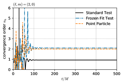
Figure 6: Convergence of the numerical solution with respect to grid resolution $h$. Plotted is the convergence index $n_{h}$, defined in Eq. (40), as a function of $t$ along a slice of constant radius $r^{*}=8.93258$ (corresponding to the right boundary of the excision tube). In the “standard” test, the analytical solution in the tube is fitted for afresh for each choice of grid resolution, and the observed steady-state convergence is linear ($n_{h}\approx 1$). For comparison, when we fix the analytical solution in the tube as we vary $h$ (“frozen fit”), the observed convergence is quadratic ($n_{h}\approx 2$), as it is for a run with an exposed point particle without an excision tube (“point particle”). The reduction in convergence rate evidently caused by the matching procedure is discussed in the text.

Next we perform our convergence test with a worldtube excision. Here we have a choice in how the array of matching points outside the tube is modified as we vary $h$. A sensible “like-to-like” comparison is one in which the physical position and pattern of the data points around the worltube is held fixed as $h$ is varied. Proceeding in this way, our convergence test with a worldtube excision yields $n_{h}\approx 1$, indicating that the convergence is only linear—see again Fig. 6 for an example. We find this deterioration in convergence rate affects all $\ell,m$ modes examined (static as well as radiative), and all model orders attempted ($n=1,2,3$). Repeating the test with a sequence of smaller $h$ values does not improve the situation, and the convergence remains linear. However, quadratic convergence is recovered if (for a static mode) we replace the regression model in the tube with the known exact analytical solution. We also recover quadratic convergence if we “freeze” the matched analytical model in the tube as we vary $h$ (i. e., fit the model using one value of $h$ and then apply the same polynomial regression model when running with the other two $h$ values participating in our convergence test).

The apparent reduction in convergence rate may be explained as resulting from a coupling between $h$-related and $R$-related errors, expected when the approximate analytical model in the tube is allowed to depend on $h$, as in our convergence test. To understand this, consider that the value of the numerical field at a point $x$ outside the worldtube is a function $\Psi(x;\tilde{h},\tilde{R})=\Psi_{\mathrm{exact}}(x)+\delta\Psi(x;\tilde{h},\tilde{R})$ depending parametrically on both $\tilde{h}:=h/m_{1}$ and $\tilde{R}:=R/m_{1}$ (we ignore here the dependence on $n$, assumed fixed for the rest of this discussion). For small $\tilde{h}$ and $\tilde{R}$, the error term may be expressed as a double Taylor expansion, $\delta\Psi=\sum_{i,j}a_{ij}\tilde{h}^{i}\tilde{R}^{j}$. The terms with $j=0$ describe the usual discretization error for $R\to 0$ (exposed point particle); we have $a_{00}=0=a_{10}$, with the leading term being $a_{20}\tilde{h}^{2}$ for our quadratically convergence code. The terms with $j\neq 0$ arise from the approximate nature of the analytical solution in the tube. According to the argument in Sec. III.3 (and as demonstrated in the next subsection), the leading finite-$R$ error is of $\mathcal{O}(R^{n})$, and it is therefore expected to have the form $\delta\Psi\simeq(a_{0n}+a_{1n}\tilde{h}+\cdots)\tilde{R}^{n}$ in general. When we construct the index $n_{h}$ in our convergence test, the contribution from the $\propto a_{0n}$ term cancels out, and $n_{h}$ is dominated by the $\propto a_{1n}$ error term, giving rise to the observed linear convergence in $h$ at fixed $R$. The crucial point here is that, in our convergence test, we allow the value of the approximate analytical model on the tube’s boundary to depend on $h$ (in a complicated way, via a matching procedure that involves numerical data points that themselves depend on $h$), and as a result the $R$-related error also becomes $h$-dependent. When we freeze the analytical model (or use the exact analytical solution for it) we decouple between the $h$-related and $R$-related errors, and quadratic convergence is recovered.

We note the occurrence of such linear-in-$h$ error terms is not necessarily a weakness of our scheme: in practice, for a particular choice of $h$ and $R$, the error term $a_{1n}\tilde{h}R^{n}$ is not necessarily numerically larger than the term $a_{02}\tilde{h}^{2}$. Rather, the occurrence of a linear term is a somewhat artificial combined feature of the particular matching procedure applied and the particular way the convergence test is designed. The lesson from the above discussion is that one should exercise caution in designing and interpreting convergence tests for a worldtube scheme, being mindful about the potential effect of coupling between finite-difference and worldtube-related sources of error.

V.2 Convergence with Worldtube Size

It is of greater interest, in the context of this work, to quantify and understand the scaling of our solutions with the tube size $R$ and model error $n$. Figures 7 and 8 show how the local finite-$R$ error in our numerical solutions varies as a function of $R$ (at fixed $n$; top panels) and as a function of $n$ (at fixed $R$; bottom panels). In Fig. 7 we measure the finite-$R$ error by comparing with the exact analytical solution for the static mode $(2,0)$ and in Fig. 8 we measure it by comparing with numerical solutions obtained using our exposed point-particle code. In both cases we display the relative differences as functions of $r^{*}$ on a late-time $t=\text{const}$ slice.

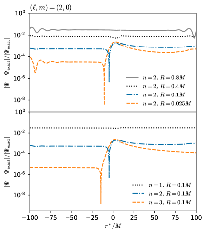
Figure 7: The relative finite-$R$ error in $\Psi_{20}$ as measured by comparison with the exact analytical solution $\Psi_{exact}$. In the upper panel we vary the tube radius $R$ at fixed model order $n=2$, and in the lower panel we vary $n$ at fixed $R=0.1M$. The relative difference is shown on a late-time $t=\text{const}$ slice. The numerical resolution is $h=0.005M$ in all cases.

Figure 8: The relative finite-$R$ error in $\Psi_{22}$ as measured by comparison with the (accurate) numerical solution $\Psi_{pp}$ from our point-particle code. The format of this plot and all other details are as in Fig. 7.

We see that, as expected, our solutions generally become more accurate as we decrease $R$ or increase $n$. We note that even with the simplest, linear ($n=1$) analytical model, and with a tube radius as large as $R=0.1M$, the worldtube-related error is only around $1\%$ almost uniformly. There is a marked reduction in error at smaller $R$ and larger $n$, except near the worldtube (at $r^{*}\approx 9M$ in these figures, too narrow to be resolved), where the error seems to saturate. As we demonstrate further below, the saturation marks the point where finite-difference error becomes dominant over $R$-related error, so that a further decrease in $R$ (or increase in $n$) does not lead to a further reduction in overall error. The effect is most pronounced near the worldtube, since the finite-difference error is largest there (where field gradients are largest), while worldtube error (we expect) remains roughly spatially uniform. The effect is exacerbated by the fact that as we decrease $R$ we expose more of the high-gradient region surrounding the particle. To fully demonstrate convergence with $R$ or $n$ near the tube would require a concurrent refinement of resolution there.

To quantity the rate of convergence with respect to $R$ (at fixed $n$ and $h$), we construct the index

$$n_{R}=\log_{2}\left|\frac{\Psi_{R}-\Psi_{\frac{R}{2}}}{\Psi_{\frac{R}{2}}-\Psi_{\frac{R}{4}}}\right|\,,$$ (41)

where $\Psi_{R^{\prime}}$ represents the value of the field calculated with a tube radius $R=R^{\prime}$. This measures the “internal” convergence of the numerical solution as we decrease $R$ (as opposed to convergence to the exact solution, illustrated in Figs. 7 and 8). Figure 9 shows $n_{R}$ as a function of $t$ along an $r=\text{const}$. We observe $n_{R}\approx n$, indicating that the dominant tube-related error is of $\mathcal{O}(R^{n})$—precisely as predicted in Sec. III.3

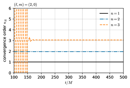
Figure 9: Convergence of the numerical solution with respect to tube size $R$, at fixed model order $n$ and resolution $h(=0.005M)$. We plot the internal convergence index $n_{R}$, defined in Eq. (41), as a function of $t$ along a fixed radius of $r^{*}=8.93258M$. To obtain $n_{R}$ (for each model order $n$) we carry out three runs with $R=0.1M$, $0.05M$ and $0.025M$. After the decay of initial junk, the convergence order appears to be $n_{R}\approx n$, indicating that the dominant tube-related error is of $\mathcal{O}(R^{n})$.

So far we have been considering “local” measures of error, ones depending on location and time. It is also informative to examine a global error norm, which we now introduce and adopt for the rest of our analysis here and in Sec. VII. We denote by $||\Psi||_{L^{1}}$ the $L^{1}$ norm of a numerical field $\Psi$ evaluated on a $t=\text{const}$ slice. The numerical data points for this norm are sampled uniformly in $r^{*}$ in the domain $[-100M,r^{*}_{p}-R]\cup[r^{*}_{p}+R,100M]$. When comparing norms corresponding to runs with different $R$ values, the largest of the $R$ values is used for all norms.

The top panel in Fig. 10 shows the value of the relative error norm $||\Psi-\Psi_{\mathrm{exact}}||_{L^{1}}/||\Psi_{\mathrm{exact}}||_{L^{1}}$ as a function of $R$ for the static mode $(2,0)$, with $\Psi_{\mathrm{exact}}$ being the exact analytical solution. We see that the error norm decreases with increasing model order $n$ and decreasing tube size $R$, but for $n=2,3$ it seems to saturate at small $R$. This behavior is consistent with what we saw in Figs. 7 and 8: when the worldtube error magnitude falls below that of the discretization error, a further reduction in tube size does not improve the accuracy of the solution. This explanation is further supported by the data shown in the lower panel of Fig. 10, where we display the internal error norm $||\Psi_{R}-\Psi_{R/2}||_{L^{1}}/|\Psi_{R/2}||_{L^{1}}$: Here we see a monotonic convergence with $R$ at a constant rate even for $n=2,3$; the field norm converges to a value that differs slightly from $||\Psi_{\mathrm{exact}}||_{L^{1}}$ due to the dominating $h$-related error.

Figure 10: Top panel: Relative $L^{1}$ error norm with respect to the exact analytical solution, as a function of worldtube radius $R$. Bottom panel: Internal relative error norm calculated by varying $R$. In both cases the finite-difference resolution is held fixed at $h=0.005$. The saturation of error in the upper panel is due to the finite-difference error becoming dominant at small $R$.

To quantify the rate of convergence of the global norm with $R$, we introduce the convergence index

$$n_{R}^{\mathrm{(norm)}}:=\log_{2}\frac{||\Psi_{R}-\Psi_{\frac{R}{2}}||_{L^{1}}}{||\Psi_{\frac{R}{2}}-\Psi_{\frac{R}{4}}||_{L^{1}}}\,,$$ (42)

plotted in Fig. 11. We observe $n_{R}^{\mathrm{(norm)}}\approx n$, i. e. the tube-related error is $\mathcal{O}(R^{n})$ also as measured by the global $L^{1}$ norm. Similar results are obtained for other $\ell,m$ modes.

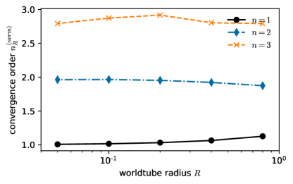
Figure 11: Convergence of the $L^{1}$ norm with respect to $R$, at fixed model order $n$ and resolution $h(=0.005M)$. We plot the internal convergence index $n_{R}^{\mathrm{(norm)}}$, defined in Eq. (42), and observe $n_{R}^{\mathrm{(norm)}}\approx n$. Thus the worldtube error scales like $\sim R^{n}$ also as measured by the global $L^{1}$ norm.

VI Scheme II: Numerical Method

VI.1 Evolution Equations

By introducing the new variables

$$\pi :=\partial_{t}\Psi\,,$$ (43)

$$\chi :=\partial_{r^{*}}\Psi\,,$$ (44)

we reduce the evolution equation (9) (in the vacuum region outside the worltube) to the first-order system

$$\partial_{t}\Psi =\pi\,,$$ (45a)

$$\partial_{t}\pi =\partial_{r^{*}}\chi-V\Psi\,,$$ (45b)

$$\partial_{t}\chi =\partial_{r^{*}}\pi+\kappa(\partial_{r^{*}}\Psi-\chi)\,,$$ (45c)

where $\kappa$ is a constraint damping parameter controlling how strongly violations of the constraint (44) are damped (see [38], where the symbol $\gamma_{2}$ corresponds to our $\kappa$). In practice we chose $\kappa=1$ for all the results presented for this scheme. We further introduce the puncture and regular fields $\pi^{\mathcal{P}}$, $\chi^{\mathcal{P}}$, $\pi^{\mathcal{R}}$, $\chi^{\mathcal{R}}$ of the reduction variables $\pi$ and $\chi$, as well as their corresponding analytical approximations in the tube, $\pi^{A}=\pi^{\mathcal{P}}+\pi^{\mathcal{R}}$ and $\chi^{A}=\chi^{\mathcal{P}}+\chi^{\mathcal{R}}$.

We now introduce auxiliary variables $\tilde{\Psi}(t)$, $\tilde{\Psi}^{\prime}(t)$ and $\tilde{\Psi}^{\prime\prime}(t)$ defined on the worldtube boundary $\partial\Gamma$, which are to act as intermediaries in conveying information to and from the approximate solution within the worldtube. These represent, respectively, the field $\Psi$, and its first and second $r^{*}$ derivatives on $\partial\Gamma$. Similarly, we introduce $\tilde{\pi}$, $\tilde{\pi}^{\prime}$ and $\tilde{\pi}^{\prime\prime}$, as well as $\tilde{\chi}$, $\tilde{\chi}^{\prime}$ and $\tilde{\chi}^{\prime\prime}$. These fields are determined by solving a set of ODEs along $\partial\Gamma$, obtained from the restriction of Eqs. (45) to the boundary:

$$\partial_{t}\tilde{\Psi} \overset{\scriptscriptstyle\wedge}{=}\tilde{\pi}\,,$$ (46a)

$$\partial_{t}\tilde{\pi} \overset{\scriptscriptstyle\wedge}{=}\tilde{\chi}^{\prime}-V\tilde{\Psi}\,,$$ (46b)

$$\partial_{t}\tilde{\chi} \overset{\scriptscriptstyle\wedge}{=}\tilde{\pi}^{\prime}+\kappa(\tilde{\Psi}^{\prime}-\tilde{\chi})\,.$$ (46c)

The symbol $$\overset{\scriptscriptstyle\wedge}{=} \partial\Gamma (\tilde{\Psi}^{\prime},\tilde{\pi}^{\prime},\tilde{\chi}^{\prime})$$ denotes equality on . The ODEs for arise from the radial derivative of Eqs. (45), restricted to the boundary:

$$\partial_{t}\tilde{\Psi}^{\prime} \overset{\scriptscriptstyle\wedge}{=}\tilde{\pi}^{\prime}\,,$$ (46d)

$$\partial_{t}\tilde{\pi}^{\prime} \overset{\scriptscriptstyle\wedge}{=}\tilde{\chi}^{\prime\prime}-\tilde{\Psi}\partial_{r^{*}}V-V\tilde{\Psi}^{\prime}\,,$$ (46e)

$$\partial_{t}\tilde{\chi}^{\prime} \overset{\scriptscriptstyle\wedge}{=}\tilde{\pi}^{\prime\prime}+\kappa(\tilde{\Psi}^{\prime\prime}-\tilde{\chi}^{\prime})\,.$$ (46f)

Finally, the ODEs for $$(\tilde{\Psi}^{\prime},\tilde{\pi}^{\prime\prime},\tilde{\chi}^{\prime})$$ arise from the second spatial derivative of Eqs. (45):

$$\partial_{t}\tilde{\Psi}^{\prime\prime} \overset{\scriptscriptstyle\wedge}{=}\tilde{\pi}^{\prime\prime}\,,$$ (46g)

$$\partial_{t}\tilde{\pi}^{\prime\prime} \overset{\scriptscriptstyle\wedge}{=}\partial_{r^{*}}^{3}\chi^{A}-\tilde{\Psi}\partial_{r^{*}}^{2}V-2\tilde{\Psi}^{\prime}\partial_{r^{*}}V-V\tilde{\Psi}^{\prime\prime}\,,$$ (46h)

$$\partial_{t}\tilde{\chi}^{\prime\prime} \overset{\scriptscriptstyle\wedge}{=}\partial_{r^{*}}^{3}\pi^{A}+\kappa(\partial_{r^{*}}^{3}\Psi^{A}-\tilde{\chi}^{\prime\prime})\,.$$ (46i)

To close the set of auxiliary ODEs, Eqs. (46h) and (46i) couple to the matched analytical approximations $\Psi^{A}$, $\pi^{A}$ and $\chi^{A}$. $\Psi^{A}$ is obtained by solving Eq. (22) using as $\partial_{r^{*}}^{j}\Psi^{N}$ the six boundary values $\tilde{\Psi},\tilde{\Psi}^{\prime},\tilde{\Psi}^{\prime\prime}$ (three each at $\partial\Gamma_{-}$ and at $\partial\Gamma_{+}$). Analogously, $\pi^{A}$ and $\chi^{A}$ are obtained using $\tilde{\pi}$, $\tilde{\pi}^{\prime}$, $\tilde{\pi}^{\prime\prime}$, and $\tilde{\chi}$, $\tilde{\chi}^{\prime}$, $\tilde{\chi}^{\prime\prime}$ respectively. The system of equations (45) are not yet coupled to the exterior (bulk) solution; this coupling will be discussed and incorporated below in Sec. VI.3.

The ODE system above yields an approximate analytical solution whose regular part is accurate through $\mathcal{O}(\Delta{r^{*}}^{5})$. In Sec. VII we also investigate setups with regular fields expanded to $\mathcal{O}(\Delta{r^{*}}^{3})$ only. For these tests we discard $\tilde{\Psi}^{\prime\prime}$, $\tilde{\pi}^{\prime\prime}$ and $\tilde{\chi}^{\prime\prime}$ and the corresponding evolution equations (46g)–(46i), and use a third-order analytical approximation to close the system. The auxiliary system could be extended to arbitrary derivative orders in an obvious way, by taking sufficiently many derivatives of the field equations. Note that the scheme can be interpreted as evolving the the regular parts only, since the puncture field and its spatial and temporal derivatives are known up to a given order through Eq. (13).

VI.2 Boundary Treatment

Boundary conditions must be provided on the outer boundaries of the computational domain and on the excision boundary $\partial\Gamma$. Furthermore, if the computational domain is divided into smaller elements, then boundary conditions are needed at the interfaces where neighboring elements meet. For the boundary implementation presented here we assume a numerical scheme that is formulated on collocation points. To derive the boundary implementation we perform a characteristic decomposition [39] of the system of PDEs. We write the system in the form

$$\partial_{t}\mathbf{u}=A^{k}\partial_{k}\mathbf{u}+\mathbf{f}(\mathbf{u})\,,$$ (47)

where $\mathbf{u}=(\Psi,\pi,\chi)$ is the vector of evolution variables, $A^{k}$ are the principal part matrices and $\mathbf{f}$ contains the non-principal terms. The characteristic vectors $\mathbf{v}$ are the left eigenvectors of $A^{k}\hat{s}_{k}$, where $\hat{s}$ is the respective outward pointing unit normal to the element boundary; here, since we work in one spatial dimension, $\hat{s}$ has only one component and the index is suppressed in the notation. The characteristic speeds $\lambda$ are the corresponding eigenvalues. The characteristic variables are the inner products of $\mathbf{v}$ and $\mathbf{u}$, i. e. for our system,

$$\begin{matrix}[l]\hat{u}^{\pm}&=\pi\pm\hat{s}\chi+\kappa\Psi~{}~{}&\lambda^{\pm}&=\pm 1\\ \hat{u}^{0}&=\Psi&\lambda^{0}&=0\,.\end{matrix}$$ (48)

Characteristic variables with positive characteristic speed are referred to as incoming and boundary conditions must be provided for them, i. e. we have to provide boundary data for $\hat{u}^{+}$. Characteristic variables with $\lambda<0$ are outgoing and no boundary condition is needed. Likewise we do not need boundary conditions for the static characteristic variable $\hat{u}^{0}$.

We modify the time derivatives of the incoming characteristic variables at the boundary points to impose boundary conditions. At the interface between elements we employ a penalty method [40], modifying the time derivative of the incoming characteristic field $\hat{u}^{+}$ in the following way:

$$\partial_{t}\hat{u}^{+}=D_{t}\hat{u}^{+}+p\lambda^{+}(\hat{u}^{+}_{\mathrm{neighbour}}-\hat{u}^{+})\,,$$ (49)

where $D_{t}$ is the time derivative constructed from the evolution equations (45), before the boundary modification has been added. Furthermore, $\hat{u}^{+}_{\mathrm{neighbour}}$ denotes the value of $\hat{u}^{+}$ on the neighbouring element (i.e. evaluated with data from the neighboring element, but still using the surface normal $\hat{s}$ pointing out of the current element) Finally, the penalty parameter $p$ is chosen to be $p=J/w$ as in [40], which guarantees stability of the method. Here $J=\partial x/\partial r^{*}$ is the Jacobian associated to transformations from the local coordinates $x$ of the element to the global coordinates $r^{*}$ of the computational domain and $w$ is the integration weight of the point at the element boundary for the quadrature on the element grid. The given expression for the penalty parameter holds for integration weights satisfying a summation-by-parts property [41] with respect to the derivative stencil of the numerical method. We now introduce

$$b_{\pm}(r^{*})=\begin{cases}1,&\mbox{if }r^{*}=r^{*}_{\pm}\\ 0,&\mbox{if }r^{*}\neq r^{*}_{\pm}\end{cases}\,,$$ (50)

where $r^{*}_{-}$ and $r^{*}_{+}$ denote the position of the element’s left and right boundary, with the corresponding boundary normals being $\hat{s}=-1$ on $r^{*}_{-}$ and $\hat{s}=1$ on $r^{*}_{+}$. The modified equation of motion can be rewritten as

$$\begin{split}\partial_{t}\hat{u}^{+}=D_{t}\hat{u}^{+}&+\left[p\lambda^{+}(\hat{u}^{+}_{\mathrm{neighbour}}-\hat{u}^{+})\right]_{r^{*}_{-}}b_{-}\\ &+\left[p\lambda^{+}(\hat{u}^{+}_{\mathrm{neighbour}}-\hat{u}^{+})\right]_{r^{*}_{+}}b_{+}\,,\end{split}$$ (51)

where the subscript on the square bracket denotes the point at which the bracketed expression is evaluated.

An alternative way to impose boundary conditions is the Bjørhus method [42], where the time derivatives are modified like

$$\begin{split}\partial_{t}\hat{u}^{+}=D_{t}\hat{u}^{+}&+\left[-\lambda^{+}(\hat{s}\partial_{r^{*}}\hat{u}^{+}-g)\right]_{r^{*}_{-}}b_{-}\\ &+\left[-\lambda^{+}(\hat{s}\partial_{r^{*}}\hat{u}^{+}-g)\right]_{r^{*}_{+}}b_{+}\,.\end{split}$$ (52)

The term $g$ models the expression for $\hat{s}\partial_{r^{*}}\hat{u}^{+}$ that one desires to impose at the boundary. At the excision and the outer boundary one can employ either the penalty or the Bjørhus method, but for the results shown here at the outer boundaries the latter is employed, whereas on the excision boundary the penalty method is used.

The modifications of the original equations (45a) are obtained after transforming back from the characteristic variables to the evolved variables.

On the excision boundary, boundary conditions for the penalty method are obtained from the matched analytical solutions,

$$\hat{u}^{+}_{\mathrm{neighbour}}=\pi^{A}+\hat{s}\chi^{A}+\kappa\Psi^{A}\,,$$ (53)

and similarly for the Bjørhus method:

$$g=\hat{s}\partial_{r^{*}}(\pi^{A}+\hat{s}\chi^{A}+\kappa\Psi^{A})\,.$$ (54)

For the static modes we find it useful to choose

$$g=\frac{\partial_{r^{*}}^{2}\Psi_{\mathrm{exact}}}{\hat{s}\partial_{r^{*}}\Psi_{\mathrm{exact}}}(\pi+\hat{s}\chi)+\kappa\hat{s}\chi\,.$$ (55)

This choice ensures that in the static case, i. e. $\pi=0$, the field has the same derivative as the exact analytical solution (12). There are other choices consistent with the analytical solution, but we find that this particular choice has small numerical reflections at the boundary.

For the radiative modes we find that for large $r^{*}$ the characteristic variables behave like $\hat{u}^{+}-\kappa\Psi\sim\exp[im\Omega(r^{*}-t)]/{r^{*}}^{2}$. Boundary conditions compatible with this functional form are given by:

$$g=\left(-\frac{2}{r}+im\Omega\right)(\pi+\hat{s}\chi)+\kappa s\chi\,.$$ (56)

Near the horizon we impose

$$g=-im\Omega(\pi+\hat{s}\chi)+\kappa\hat{s}\chi\,,$$ (57)

corresponding to the behaviour $\hat{u}^{+}-\kappa\Psi\sim\exp(im\Omega(-r^{*}-t))$.

VI.3 Coupling to the Boundary Ordinary Differential Equations

Besides coupling the auxiliary ODEs to the bulk PDEs one also needs a prescription for the opposite direction, i. e. some external input for the auxiliary system, Eqs. (46). A stable system can be derived realizing that the auxiliary system is equivalent to a spectral method employed inside the excision worldtube. This means we can employ the same techniques as before when imposing boundary conditions, i. e., we will modify each block of Eqs. (46) with extra terms in the spirit of Eq. (51) –if the penalty method is chosen– or Eq. (52), if the Bjørhus method is used. The necessary right-hand-side modifications are constructed by assuming a fiducial spectral element spanning the worldtube $\Gamma$ on which the functions $b_{\pm}$ are evaluated. On the fiducial element we collocate grid points employing a Chebyshev-Gauss-Lobatto [43] collocation scheme with the number of grid points chosen to be consistent with the order of expansion of the regular field, i. e. one grid point more than the order.

The boundary data in the modification terms for the penalty method, Eq. (49), is given simply by the values of the bulk fields

$$\hat{\tilde{u}}^{+}_{\mathrm{neighbour}}=\hat{u}^{+}|_{r^{*}_{\pm}}\,.$$ (58)

Similarly in the case of the Bjørhus method, Eq. (52), one uses the derivatives of the bulk fields,

$$\tilde{g}=\hat{s}(\partial_{r^{*}}\pi|_{r^{*}_{\pm}}+\hat{s}\partial_{r^{*}}\chi|_{r^{*}_{\pm}}+\kappa\chi|_{r^{*}_{\pm}})\,.$$ (59)

Denoting by $C$ the square bracket expressions in either (51) or (52), the corresponding modifications in the auxiliary system are given by

$$\partial_{t}\hat{\tilde{u}}^{+} =D_{t}\hat{\tilde{u}}^{+}+C_{r^{*}_{-}}b_{-}+C_{r^{*}_{+}}b_{+}\,,$$ (60)

$$\partial_{t}\partial_{r^{*}}\hat{\tilde{u}}^{+} =D_{t}\partial_{r^{*}}\hat{\tilde{u}}^{+}+C_{r^{*}_{-}}\partial_{r^{*}}b_{-}+C_{r^{*}_{+}}\partial_{r^{*}}b_{+}\,,$$ (61)

$$\partial_{t}\partial_{r^{*}}^{2}\hat{\tilde{u}}^{+} =D_{t}\partial_{r^{*}}^{2}\hat{\tilde{u}}^{+}+C_{r^{*}_{-}}\partial_{r^{*}}^{2}b_{-}+C_{r^{*}_{+}}\partial_{r^{*}}^{2}b_{+}\,.$$ (62)

The system generalises in an obvious way to higher orders by taking higher and higher derivatives in $r^{*}$, and it is understood that $C_{r^{*}_{\pm}}$ are constants with respect to $r^{*}$. When employing the penalty boundary conditions (49), the penalty parameter contained in $C_{r^{*}_{\pm}}$ is determined from the fiducial worldtube element grid. As for the boundary modifications of the bulk PDEs, the modifications of the ODE system (46) are obtained by transforming back from the characteristic variables to the evolved variables.

VI.4 Implementation Details

We evolve Eqs. (45) and (46) using the classic fourth-order Runge–Kutta method on the spatial domain $[-300M,300M]\setminus\Gamma$, where the worldtube $\Gamma$ is centered on the position $r_{p}^{*}$ of the particle. The numerical domain is divided into a set of spectral elements. On each element field values are expanded into a series of basis polynomials and on every element the series is truncated at the same order. For the results presented here, Chebyshev polynomials are used as the spectral basis and the grid is collocated on Chebyshev-Gauss-Lobatto points. Details on how the method works can be found in [43], which we mostly followed for our code.

For the evolution of the system to be stable, the time step has to satisfy a CFL condition, where the relevant length interval is given by the minimal interval $\Delta r^{*}_{\mathrm{min}}$ between collocations points. Henceforth we chose the time step to be $\Delta t=c_{\mathrm{CFL}}\Delta r^{*}_{\mathrm{min}}$, where it is important that the fiducial element, which was introduced for the coupling to the auxiliary boundary system, is also taken into account in the determination of $\Delta r^{*}_{\mathrm{min}}$. The constant $c_{\mathrm{CFL}}$ is set to $0.5$ for static setups ($m=0$ modes), whereas for the evolution of radiative modes we chose $c_{\mathrm{CFL}}=0.25$, which we have checked to be sufficiently small for the results in our setups to be converged with respect to $\Delta t$. Furthermore, we note that the matching must be performed at every Runge-Kutta substep, i. e. in every right-hand-side evaluation. Otherwise the scheme does not converge with fourth order with respect to $\Delta t$.

For radiative modes it is important to treat the phase factor $e^{-im\Omega t}$, which is implicit in $S_{\ell m}(t)$ in Eq. (13), with high numerical precision. Because of the high precision of the spectral scheme, we are sensitive to machine round-off in the argument of the phase factor. If we were to use the total time $t$, the round-off error would grow linearly with $t$ and thus affect the precision of the phase factor as well. Instead we use an approach where after every time step $\Delta t$ we multiply the phase factor by $e^{-im\Omega\Delta t}$ to update it for the next time step, and normalise the result such that the norm of the phase factor remains exactly 1. The same updating procedure is employed for the individual Runge-Kutta substeps, so that the phase factor corresponds to the respective time of the substep. Furthermore, we use quadruple precision in evaluating the evolution time. We find this necessary to ensure that our convergence tests are not limited by round-off error in the time at which different configurations are compared.

VII Scheme II: Tests and analysis

VII.1 Test Setups

We investigate the scheme with two different matching setups, which differ by the polynomial order of the matched regular field inside the worldtube. We test one setup where the regular field is expanded to fifth order and the auxiliary system is evolved using the evolution equations as stated in Sec. VI. In the second setup the regular field is expanded to third order only and the auxiliary system is evolved using Eqs. (46a)–(46f), with $\tilde{\Psi}^{\prime\prime}$, $\tilde{\pi}^{\prime\prime}$, $\tilde{\chi}^{\prime\prime}$ replaced by their analytical approximations to close the system. The expansion of the puncture field varies from second to fifth order and hence the second setup can probe a situation where the truncation error is dominated by the regular field, whereas the first setup always makes sure that the error in the puncture field converges slower or as fast as the regular field. Combined these setups allow us to distinguish between the convergence behaviour stemming from the truncation of the puncture expansion and the one stemming from the expansion of the regular field.

We use a numerical resolution of 15 grid points per spectral element and up to 256 spectral elements covering $r^{*}$ values in the interval $[-100,300]\setminus[r_{p}^{*}-R,r_{p}^{*}+R]$. Because the numerical domain changes when the worldtube radius is changed we always compute norms on the reference $r^{*}$ interval covering values $[-100,300]\setminus[r_{p}^{*}-2M,r_{p}^{*}+2M]$ to ensure comparability. For the internal convergence tests we interpolate all solutions on a common reference grid before subtracting the different solutions. This accounts for the change of grid collocation when the resolution or the worldtube radius is changed.

We first test the scheme for the static mode $\ell=2,m=0$, with the scalar charge in a fixed circular geodesic orbit with $r_{p}=7M$ (as for Scheme I). As initial data for the evolution, the static analytical solution (12) is used. Because of the finite-resolution truncation error, the numerical solution does not settle to the precise analytical solution, but to a slightly different one. The transition from the analytical initial data to the numerical static solution causes transient radiation propagating off the numerical domain, with a small partial reflection at the outer domain boundaries. After a coordinate time of $\sim 5000M$ much of the transient radiation has decayed and the difference with the analytical solution saturates. The numerical data at this time is taken as the representation of the numerical static solution.

Figure 12 shows the relative difference between the numerical and analytic solution. The small differences are amplified at large $r^{*}$, because they are normalised by the solution which approaches zero in this limit. The data shows that the numerical solution does not settle down completely, but that there remains some residual numerical noise propagating on the grid, which can be attributed to the finite machine precision. We have also tested the numerical scheme with different initial data and find that it settles down to the same static solution. However, in that case the transient radiation has a larger amplitude and takes longer to decay.

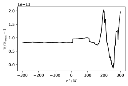
Figure 12: Relative error of the $Y_{20}$ mode for 15 points per element using the 5th order expansions for the puncture and regular field, and a worldtube radius of $R=0.1$.

To test the convergence with $R$ in a non-static situation we investigate the $\ell=4,m=4$ mode, with the charge again being fixed at $r_{p}=7M$. For these modes there is no solution known in analytical form and hence we start with zero initial data, i. e. $\Psi=0,\dot{\Psi}=\pi=0$. Furthermore we estimate the error by taking the difference between two runs that differ in the size of their worldtubes by a factor of two. As in the static case, there is some transient radiation that is radiated away until the system settles down to a stationary state. The presence of this junk radiation is partially obscured by the periodic changes in $\Psi$, but it can be observed when taking the difference of the modulus $|\Psi|$ of two simulations with different worldtube size. Figure 13 shows the estimated relative error for the highest resolution used in our results. It can be observed that the error on the left side of the particle is dominated by numerical noise, whereas on the right the difference between the two runs looks smooth and is modulated by the periodic waveform of the signal. The noise on the left side can be attributed to an insufficient resolution, which is amplified by the relatively small modulus $|\Psi|$ in that area; cf. Fig. 2.

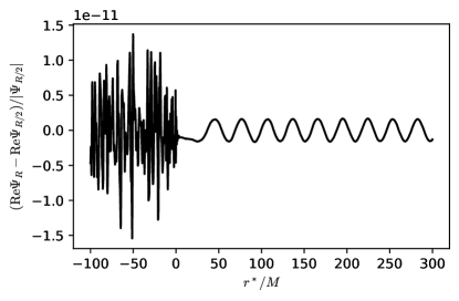
Figure 13: Relative error of the $Y_{44}$ mode for 15 points per element using the 5th order expansions for the puncture and regular field and a worldtube radius of $R=0.05$. The data is taken for the stationary end state at $t=11000M$.

VII.2 Convergence Tests

Figure 14 shows the error as a function of the number of collocation points per spectral element and demonstrates the exponential convergence of our spectral discretisation scheme. The error levels off at high number of points, because error contributions in the matched analytical solution inside the worldtube become the dominating source of error. Next the convergence with respect to the size of the worldtube is tested. In these tests we report only error quantities that are fully converged with respect to the number of collocation points and the matched analytical solution is the only source of error.

Figure 14: Error of the $Y_{20}$ mode as a function of the number of points per spectral element. The grid consists of 128 elements and a has worldtube radius of $R=0.2$. The puncture and regular parts of fields are expanded to 5th order.

Figure 15 demonstrates the convergence of the first setup, where the matched regular fields are all expanded up to order five. It shows the $L^{1}$ norm of the difference to the exact analytical solution, along with the corresponding convergence order $n_{R}^{\mathrm{(norm)}}$ defined in Eq. (42). For even expansion orders $n_{\mathcal{P}}$ of the puncture field, the total scheme converges with $n_{\mathcal{P}}$ as predicted from the analysis in Sec. III.3, whereas for the odd orders the convergence is one order higher. It is not known to us what causes this irregular convergence pattern with respect to $n_{\mathcal{P}}$, but this finding suggests that the $\partial_{n}\Psi^{N}$ term in Eq. (27) is suppressed for odd $n_{\mathcal{P}}$.

We can not only observe a decrease in the error with decreasing worldtube size, but also with increasing order of the puncture expansion. The error for 3rd and 4th order, however, are almost identical in their magnitude. The reason for this particular behaviour is unknown to us.

Figure 16 shows the convergence behaviour of the second setup. For the cases where the expansion order of the puncture is in the range from two to four we find convergence consistent with the findings of the first setup. However, for a puncture expansion order of five the convergence order is limited by the regular solution. Since the regular field is truncated at third order in this setup, the analysis of Sec. III.3 would predict a convergence order of only three and disregarding the $\partial_{n}\Psi^{N}$ terms a convergence order of four, but it is observed that the convergence is actually of fifth order. This apparent super-geometric convergence could be explained by the fact that it is not only the field $\Psi^{\mathcal{R}}$ that is expanded to third order, but also the derivative $\chi^{\mathcal{R}}$. Since the third order coefficient of $\chi^{\mathcal{R}}$ corresponds to the fourth order coefficient of $\Psi^{\mathcal{R}}$ this could lead to a scheme where the effective expansion order of the regular field is one order higher than naively expected.

The radiative modes exhibit an error convergence behaviour that is qualitatively identical to the static modes. For completeness we show the corresponding convergence behaviour in Figs. 17 and 18.

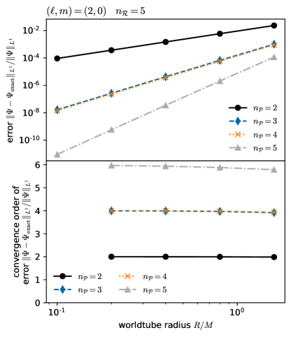
Figure 15: Top panel: $L^{1}$ norm of the difference to the analytical static solution with respect to the worldtube radius $R$ for the $Y_{20}$ mode. The indicated order $n_{\mathcal{P}}$ denotes the order of expansion of the puncture field $\Psi^{\mathcal{P}}$. The regular fields are all expanded to order five. Bottom panel: Convergence order for the $L^{1}$ norm.

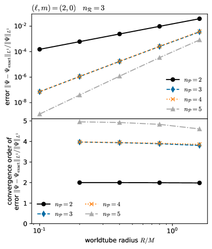
Figure 16: Top panel: $L^{1}$ norm of the difference to the analytical static solution with respect to the worldtube radius $R$ for the $Y_{20}$ mode. The indicated order $n_{\mathcal{P}}$ denotes the order of expansion of the puncture field $\Psi^{\mathcal{P}}$. The regular fields are all expanded to order three. Bottom panel: Convergence order for the $L^{1}$ norm.

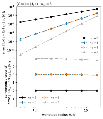
Figure 17: Top panel: $L^{1}$ norm of the difference between solutions with worldtube radius $R$ and $R/2$ for the $Y_{44}$ mode. The indicated order $n_{\mathcal{P}}$ denotes the order of expansion of the puncture field $\Psi^{\mathcal{P}}$. The regular fields are all expanded to order five. Bottom panel: Convergence order for the $L^{1}$ norm.

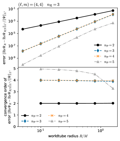
Figure 18: Top panel: $L^{1}$ norm of the difference between solutions with worldtube radius $R$ and $R/2$ for the $Y_{44}$ mode. The indicated order $n_{\mathcal{P}}$ denotes the order of expansion of the puncture field $\Psi^{\mathcal{P}}$. The regular fields are all expanded to order three. Bottom panel: Convergence order for the $L^{1}$ norm.

VIII Conclusion

Numerical simulations of binary black holes are increasingly costly with more extreme mass ratio $q$, because the CFL instability forces a reduction of the evolution time step $\Delta t\lesssim m_{2}\propto q$. This article explores a new technique to circumvent the time step limitations that arise from solving the field equations fully numerically in the region of spacetime near the small mass $m_{2}$. We place a worldtube of radius $R\gg m_{2}$ around $m_{2}$. Inside this worldtube, we replace the fully numerical solution by a perturbative solution while retaining a fully numerical solution outside the worldtube. Thus, the smallest length scales remaining on the numerical grid are of order $R$, and the CFL limit is relaxed to $\Delta t\sim R$.

The present article explores the toy problem of computing the scalar field generated by a point-charge orbiting a Schwarzschild black hole on a circular orbit. The solutions of this problem are illustrated in Fig. 2. We explore two different algorithms to match the perturbed solution inside the worldtube with the fully numerical solution outside, a matching scheme that fits over an extended region, and a boundary scheme that imposes conditions precisely at one radius. We furthermore explore two different numerical implementations for the numerical exterior solution, one based on finite differences on a characteristic grid, the other on spectral methods on spatial hypersurfaces. The most accurate solutions are obtained with the spectral scheme, which allows significantly smaller discretisation errors than the finite-difference scheme.

We achieved stable evolutions in both schemes. We also established convergence of the results in various quantities: in the grid spacing of the numerical domain, in the radius $R$ of the worldtube, as well as in the order of the approximate perturbative solution inside the worldtube. Of primary concern is convergence with worldtube radius $R$. For the finite-difference scheme, Fig. 10 demonstrates convergence $\propto R^{n}$ for a perturbative solution of order $n$. For the spectral scheme, Figs. 15 and 17 demonstrate up to sixth-order convergence in $R$.

For a worldtube radius of $R=0.8M$, we achieve relative errors $\lesssim 10^{-6}$ for a fifth-order perturbative solution, and $\approx 10^{-4}$ for a third-order internal solution. This level of accuracy at such large worldtube radius is encouraging for our ultimate goal, the application of the worldtube scheme to full GR.

The work in this paper has focused on the implementation of the worldtube architecture and exploration of matching approaches, thus demonstrating in principle that the proposed worldtube excision method works.

Future steps include 3+1D simulations of the scalar-charge problem, extending over the 1+1D simulations presented here. Such simulations will first proceed with the charge on a fixed circular orbit, and subsequently they will include scalar self-force effects resulting in an inspiral of the scalar charge. These steps will provide valuable additional insights needed to address our ultimate goal, the full binary black hole problem in GR at intermediate mass ratios.

We expect much of our methodology to carry over to those more complex cases, but with some foreseeable differences and challenges. In the 3+1D scalar toy problem, in local Fermi coordinates $(t,x^{i})$ centered on the scalar charge, the scalar field has the form $\Phi=\Phi^{\mathcal{P}}+\Phi^{\mathcal{R}}$ with [34]

$$\Phi^{\mathcal{P}}=\frac{e}{s}-\frac{e}{6s}\mathcal{E}_{ij}(t)x^{i}x^{j}+\mathcal{O}(s^{2}).$$ (63)

Here $s=\sqrt{\delta_{ij}x^{i}x^{j}}$ is the distance from the particle, and $\mathcal{E}_{ij}=R_{titj}$ (evaluated on the particle) is the tidal field due to the large black hole. This local solution takes the place of our 1+1D local solution (16) [with Eq. (13)]. All the unknowns in the 3+1D local solution are contained in $\Phi^{\mathcal{R}}$, just as in our 1+1D calculation, and after transforming the local solution to whatever external coordinates are convenient, our matching approaches should apply with little or no fundamental change.

More significant differences appear in the full gravity problem, where the local solution will instead be the metric of a tidally perturbed black hole. In local coordinates centered on the small black hole, a typical component has the form

$$g_{tt}=-(1-m_{2}/s)+e_{1}(m_{2}/s)\mathcal{E}_{ij}x^{i}x^{j}+\mathcal{O}(s^{3}/\mathcal{R}^{3})$$ (64)

for some function $e_{1}(m_{2}/s)$ [25, 28], where $m_{2}$ is the black hole’s mass. Here $\mathcal{E}_{ij}$ is now an effective tidal field that can only be determined through a matching procedure; due to nonlinearities, it is influenced by the small black hole’s own effect on the external geometry [44]. The $m_{2}/s$ term in $g_{tt}$ plays the role of the $e/s$ term in $\Phi^{\mathcal{P}}$, but as mentioned in Sec. III, beyond that term the metric does not have a neat decomposition into singular and regular pieces. Due to the $m_{2}/s$ dependence in $e_{1}$, the tidal term is singular at $s=0$. A regular piece can still be constructed by setting explicit appearances of $m_{2}$ to 0, yielding a metric with components of the form $g^{\mathcal{R}}_{tt}=-1+\mathcal{E}_{ij}x^{i}x^{j}+\mathcal{O}(s^{3}/\mathcal{R}^{3})$, which is a smooth vacuum solution analogous to $\Phi^{\mathcal{R}}$. But the remainder $g^{\mathcal{P}}_{\alpha\beta}=g_{\alpha\beta}-g^{\mathcal{R}}_{\alpha\beta}$ does not satisfy a simple field equation. Any such field equation will involve complicated nonlinear dependence on $g^{\mathcal{R}}_{\alpha\beta}$, such that $g^{\mathcal{P}}_{\alpha\beta}$ cannot be determined without simultaneously determining $g^{\mathcal{R}}_{\alpha\beta}$. This should not pose a problem for us because, by design, our matching approaches allow us to match the total metric to the external solution rather than solving field equations for a residual field as in a traditional puncture scheme discussed in Sec. III.3.

A more pronounced practical complication in the gravity problem is that we will not know in advance the transformation from the local coordinates of Eq. (64) to the coordinates used in the external numerics. The transformation must be determined as part of the matching procedure. Likewise, the motion of the small black hole must be determined dynamically through matching. We leave these challenges for future work.