Logistic growth on networks: exact solutions for the SI model
Abstract
The susceptible-infected (SI) model is the most basic of all compartmental models used to describe the spreading of information through a population. Despite its apparent simplicity, the analytic solution of this model on networks is still lacking. We address this problem here, using a novel formulation inspired by the mathematical treatment of many-body quantum systems. This allows us to organize the time-dependent expectation values for the state of individual nodes in terms of contributions from subgraphs of the network. We compute these contributions systematically and find a set of symmetry relations among subgraphs of differing topologies. We use our novel approach to compute the spreading of information on three different sample networks. The exact solution, which matches with Monte-Carlo simulations, visibly departs from the mean-field results.
I Introduction
The dynamical processes of information spreading through a population via individual interaction is ubiquitous in Nature and society [1, 2, 3, 4, 5, 6, 7], and their importance is demonstrated by the recent COVID-19 pandemic [8, 9, 10]. Typically, there are two approaches to formulate spreading processes: a collective approach based on deterministic compartmental models governing the state of the population as a whole [11, 1, 12, 13] and a more detailed approach aimed at describing the stochastic individual interactions [14, 15, 16]. Various approximation and numerical schemes have been used to solve compartmental models of epidemic spreading, and in certain cases, exact results are known [17, 18, 19, 20]. These models are effective and often give a good estimate of the temporal evolution of the system. However, they are insensitive to the connectivity properties of the individuals within the population. To take this into account, stochastic models of epidemic spreading on networks have been proposed and studied extensively over the past decades [14, 21, 22, 23, 24, 25, 26, 27, 16, 28, 29, 30, 31, 32]. Nonetheless, the presence of dynamical correlations and the non-linear nature of spreading processes make mean-field approximations and numerical simulations a necessity, while exact solutions in network epidemiology remain a rare treat [33, 34, 35, 36].
In this paper we present a general framework to describe the spreading process on a network, which allows for exact analytic solutions. We focus on the most basics and yet relevant [37, 38] of all spreading processes, the si system. The nodes of the network are either susceptible (s) or infected (i) and, by a Poisson process, infected nodes can infect their susceptible neighbors. While the compartmental model for this system is solved by the Verhulst logistic function [39], to the best of our knowledge, exact solutions to the stochastic network model are still unavailable. Here we intend to fill this gap, while simultaneously introducing a general procedure applicable to other, more complex, spreading processes.
Our exact treatment of the si system relies on the formulation of [40], inspired by many-body quantum systems. Time-dependent expectation values of target nodes (sinks), given an initial configuration of infected nodes (sources), can be obtained as a diagrammatic expansion over subgraphs of the network. Each subgraph represents a contribution to the spreading process from the sources to the sinks. We present a systematic way to compute these contributions as functions of time and furthermore, we find a set of symmetry relations among subgraphs of different topology, which simplifies the computational task. We illustrate our methods by analytically solving the spreading dynamics on three sample networks. The result differs visibly from the individual-based mean-field approximation, but agrees with Monte-Carlo simulations.
II The formalism
Consider an unweighted and undirected network of nodes, each of which can be in one of two states: s or i. These states can be used as an orthonormal basis for a two-dimensional (2D) vector space, such that 111We use a bra-ket notation for column vectors and row vectors , such that their contraction is denoted as . :
| (1) |
The network as a whole can be in possible configurations , each of which has an associated vector constructed as the tensor product of individual state vectors (1)
| (2) |
where each state }. The probabilities for the network to be in configuration at time are the components of a -dimensional probability vector
| (3) |
This vector has unit -norm by normalization of probability, which we will denote as , where denotes the flat state. The si spreading is a Markovian process and hence the probability vector evolves in time by a master equation:
| (4) |
The infinitesimal generator is a -dimensional matrix containing the possible transitions induced between neighboring states in a network with adjacency matrix . It can be constructed from tensor products of 2D matrices, which act as linear operators on the individual state vectors. In the case of the si-model, it is given by [40]:
| (5) |
The -dimensional matrices and are constructed by taking the tensor product of 2D identity matrices with the projection operator inserted at site and the infinitesimal stochastic matrix inserted at site , respectively, and:
| (6) |
Each term in performs the following local operations on the individual nodes connected by an edge: checks whether node is infected, by projecting it to the infected basis vector . The matrix simultaneously acts on node and maps the state to the infinitesimal stochastic state . This state with vanishing norm subtracts probability for the node to remain in the susceptible state and adds probability of it being infected.
Our goal is to compute the probability for a certain sink node to be infected at time , given a fixed configuration of initially infected source nodes at time .
| (7) |
We will show in section IV below how this quantity can be expressed as a sum over subgraph diagrams with specific node configurations. Terms where any node other than are in the infinitesimal stochastic state will vanish due to the contraction with the flat state . Therefore, the function will only receive contributions from terms where no node other than is in an infinitesimal stochastic state. We can hence identify the sinks of the spreading process with nodes in an infinitesimal stochastic state. Before proceeding to the diagrammatic expansion of (7), we will discuss how to this formula is derived from a dynamical partition function.
III Dynamical Partition function
In this section, we will give an expression for the dynamical partition function [42, 43] in the ensemble average over all possible trajectories of the spreading process. We will use this to derive equation (7), as well as expressions for higher-order moments. The partition function is defined as the moment generating function for the observables , which tracks whether node is infected at time .
| (8) |
Where here if node is infected at time and otherwise. The dynamical partition function depends on a set of (dual) variables , which serve as chemical potentials for the observables . The expectation value for the joint probability of nodes to be infected at time is obtained from (8) by derivation with respect to , followed by setting all :
| (9) |
The dynamical partition function (8) can be computed by summing over all microscopic configurations , where gives 1 only if node is infected in the configuration . In the vector notation , we can express as a linear operator which places a factor for each infected node in the configuration . This operator is a -dimensional diagonal matrix with the following product form:
| (10) |
Now (8) can be written as the -norm of the contraction of with the probability vector :
| (11) |
By plugging (11) in (9), one obtains the expression
| (12) |
Specifically, the probability for individual nodes to be infected at time is (7). From the dynamical partition function (11) it also follows that all higher moments of are equal to the expectation value , since:
| (13) |
Here we have used the fact that the projection operator is idempotent, i.e. . This implies that knowledge of the single node expectation values is sufficient to compute all higher-moments for the single nodes. Hence, the variance for individual nodes is:
| (14) |
For this reason we will focus in the remainder of the text on computing the single node expectation values (7).
The expectation value for the prevalence in the whole network is obtained by averaging (7) over all nodes
| (15) |
This can be obtained from a dynamical partition function by setting for all in (8):
| (16) | ||||
| (17) |
By using the link between (8) and (16), it is also possible to express the variance of the prevalence in the ensemble average over trajectories as:
| (18) |
Unlike with the variance for individual nodes (14), the total variance depends on the joint probability for nodes and to be infected simultaneously for all node pairs. In the diagrammatic expansion, these terms receive contributions from diagrams where both and are infinitesimal stochastic nodes (sinks). Higher-order moments are also obtainable from this formalism, but in this paper we will focus only on single node expectation values.
IV Diagrammatic expansion
We will now present a systematic procedure for computing the single node expectation values (7). Its expression depends on the time-dependent probability vector . By the master equation (4) we can express it as , where the initial state vector corresponds to the initial configuration of sources and susceptible nodes. The probability vector can be expanded as:
| (19) |
Here henceforth, we adopt a graphical notation to represent the action of the operators , appearing in the infinitesimal generator . We suppress displaying any susceptible nodes, as they have not been acted upon by either of the operators; we denote infected nodes as white circles, and sinks as blue ones:
| (20) |
Any source node will be displayed as a crossed-out white node: . The local operators and in (6) act on the colored and susceptible nodes as:
| (25) | ||||||||
| (30) |
In addition, the operator adds a directed edge pointing from to as specified by the adjacency matrix . The expansion (19) can now be organized as a perturbative series of directed diagrams with an increasing number of edges. When starting from an initial configuration with a single source node, the most general diagrammatic expansion for subgraphs with up to three edges reads:
| (40) |
Where the dots denote diagrams with more than three edges. Here each diagram graphically represents a vector . The combinatorial coefficient counts the number of ways can be constructed by applications of on the initial configuration, up to a sign discussed below. The vector is created as the tensor product of the displayed nodes states, times all the suppressed susceptibles . Subgraph diagrams of the displayed topology can appear in the network with a multiplicity, which is accounted for by the sum over subgraphs (s.g.) in the above equation. Depending on the network some of the diagrams might not appear in the expansion, i.e. their multiplicity is zero.
V Dynamics of the SI system.
To compute the sum over in (40) we must obtain the coefficients for each diagram. To solve this combinatorial problem we consider the action of on an arbitrary diagrams state vector . This defines four rules from which diagrams with edges are constructed from ‘parent diagrams’ with edges. Two rules govern the addition of new nodes to the diagram:
-
Rule 1:
If acts on a new susceptible node and on a white node, a new sink is attached to the white node by a directed edge.
-
Rule 2:
If acts on a new susceptible node and on a blue node, the latter node is turned white and a new sink is attached to it.
In addition, internal edges between non-susceptible nodes are added to the diagrams by two more rules:
-
Rule 3:
When acts on a blue node and on a white node, an edge is added from the latter to the former node and a minus sign appears
-
Rule 4:
When acts on a blue node and acts on a blue node, this node is turned white and a minus sign appears
Diagrammatically, examples of these rules are:
| (43) | |||||
| (46) | |||||
| (49) | |||||
| (52) |
When following the third rule, the operators and could act on a node pair which are already connected. This operation does not change the number of edges in the diagram, only the sign of the coefficient. It implies that receives a contribution , where is the number of edges ending in sinks. Together with the contributions from parent diagrams we can derive a recursive relation for :
| (53) |
with
| (54) |
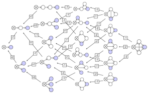
Here denotes the set of parents of the graph and gives the multiplicity and sign of the corresponding parental relationship. The set is obtained by tracing the rules (43)-(52) backwards, and contain only diagrams with one less edge ending a blue node. The collection of all possible diagrams can be thought of as a weighted directed graph of diagrams, where edges represent the childparent relationships and the edge weights correspond to the in (54). We display this graph of diagrams explicitly for all possible diagrams with four nodes in figure 1.
Equation (53) can be solved iteratively. To this end, it is convenient to express each diagram as a function of by performing the sum over in (40). If we define
| (55) |
for each diagram, the recursion relation (53) becomes a differential equation
| (56) |
with the initial condition , except when , for which . The solution for a diagram is given by
| (57) |
So any diagrams contribution to the probability vector (40) can be explicitly computed from knowledge of the contributions of parent diagrams. As the parent diagrams necessarily have one edge less, we can compute all contributions systematically by starting from the smallest possible diagram: a single source node. The expectation value in (7) is then obtained by summing the contributions for all subgraphs with fixed source, where the node is the only sink in .
V.1 Simple example - network
Let us present and work out a simple example: the complete graph with three nodes . We suppose that one of the three nodes is the initially infected source node. There are then four terms in the expansion of (40):
| (58) |
To obtain the contributions corresponding to each of these diagrams we can explicitly compute the integral (57), following the graph of parental relationships in figure 1. The first diagram only receives contributions from the single source node. We will denote its contribution as a function of by the diagram itself, appended by :
| (59) |
Here we have used the initial condition . The next two diagrams in (58) can be derived from this result as
| (61) | ||||
| (63) | ||||
| (64) |
The final diagram receive parent contributions from both these diagrams, with a relative sign due to (49) and (52):
| (68) | ||||
| (69) |
The infected expectation value for each of the two initially susceptible nodes receives contributions only from subgraphs where the node of interest is blue. This can now be computed from the above contributions as:
| (73) | ||||
| (74) |
While the loop contribution is a strictly negative function, it is balanced by two positive contributions corresponding to the two ways to reach the sink node in the loop diagram. Only the sum over all three diagrams corresponds to a probability and is hence bounded between and . Using equations (15) and (18) it is straightforward to compute the prevalence and variance for the network.
V.2 Diagram properties
For any diagram, will be monotonically increasing (or decreasing) and converge to a positive (or negative) integer for . Hence, each diagram possesses a sign, which determines whether its contribution is strictly positive or negative. This sign can be derived by the following argument: consider a diagram with nodes (of which initial infected) and edges. The action of the generator creates a directed edge between two nodes, and may change their state through the action of the operators and . The in-degree for node counts the number of times this node has been acted upon with . There is no sign change when acts on a susceptible node, but after the node is turned blue any consequent action of on the node produces a minus sign. If the node is ultimately projected upon by , no further sign changes occur. Hence the sign contribution from each white or blue node is . The total sign of the diagram is then the product over all blue and white nodes, which can be written as
| (75) |
Here we have used the fact that initially infected nodes have no incoming edges, so the sum over all in-degrees of white and blue nodes equals the total number of edges in the diagram, .
In the above derivation, we are assuming that the subgraph has only single directed edges. For larger graphs, diagrams with double directed edges can appear, as there could be several paths from sources to sinks through a particular edge. The first example of a double directed diagram is:
| (76) |
The double directed edge implies that some of the parents of this diagram have the arrow pointing one way, while other parents have it in the other direction. In this case, when computing the sign of the diagram, the double directed edges should be counted only once, and hence in (75) represents the total number of edges of the undirected diagram.
The expectation value receives contributions from all subgraphs where node is the only sink. This sum is, by construction, bounded between 0 and 1, even though the individual terms may not be. In fact, the individual contributions to do not correspond to a probability. Some diagrams have strictly positive contributions and others have strictly negative contributions. In appendix A we prove that in the limit of infinite time, the diagrams contributions converge to a finite integer value :
| (77) |
where denotes the number of valid orientations the double directed arrows in the diagram can take on. (For example, for (76) as the double directed arrow can point both up or down.) Since (77) can take on any integer value, it is clear that only the final sum over all contributing diagrams is bounded as a probability; the individual contributions will conspire to balance negative contributions with positive ones.
The number of subgraphs contributing to the expansion (40) grows quickly with the number of edges. However, not all diagrams will give independent and new contributions. We have found and proven a set of symmetry relations and decomposition rules on the diagrams which we will now discuss.
VI Symmetry relations
The dynamics of the si system gives rise to a number of relations between the contributions of different diagrams. For notational simplicity, each diagram below will now immediately represent its function .
VI.1 Reverse the flow: sources sinks
The first relation states that is equal, up to a sign, to , where is obtained from by transforming all of its sources into sinks and all of its sinks into sources.
| (78) |
Here denotes any arbitrary directed subgraph consisting solely out of white nodes. This relation states that the flow of information from source to sink is invariant under changing the direction of the flow, up to a possible sign.
Some of the first non-trivial instances of this relation are
| (81) |
and:
| (82) |
The invariance under reversal of the flow of the diagram can be understood from the way the diagrams are constructed. For each edge in the diagram, a single operation of must have been applied to construct the edge from to 222We assume the underlying network topology has only undirected edges, such that . If we replace , then the diagram of the same topology is constructed by applying to the node pairs , creating the same edges in the opposite direction. Since the total number of operations to create this inverted diagram is unchanged, the only difference between the two contributions can be a sign. The sign arises because to obtain the flipped diagram the operator may act on a different number of blue nodes. Specifically, from (75), by reversing the flow the contribution gets a minus sign if the difference is odd.
An extension of the above rule exists for diagrams whose only parents are related by the above symmetry relation. For instance, since the parents of the first two diagrams below satisfy the relation (81), it follows that:
| (83) |
where the last diagram is obtained from the second by again reversing the flow. This relation generalizes to any diagram consisting out of a node chain with an arbitrary subgraph in the middle. For any , we have diagrammatically:
| (85) | |||
| (88) |
Here represents an arbitrary graph consisting solely out of white nodes.
VI.2 Merging/separating sources and sinks
The second relation states that, for a graph with sources of degree one, each connected to distinct nodes, where is obtained from by merging all sources into a single source of degree :
| (91) |
By the first relation (78) this implies that also sinks can be merged into one, now producing the sign :
| (94) |
In the above equalities, the subgraph can in principle contain other sources or white nodes, but it must contain at least one sink; contrarily, the subgraph must contain at least one source but it can contain other white or blue nodes.
Two elementary examples of this rule are:
| (97) | ||||
| (100) |
A consequence of this relation is that diagrams containing multiple branches from the source node can be factorized into the product of the branches. For instance, the last diagram above can be further decomposed by separating the two branches from the source node, resulting in two disconnected diagrams. The diagram contribution thus factorizes into the contributions from the branches:
| (101) |
In general, any diagram containing multiple branches from the source node factorizes into the product of the branches. Graphically:
| (102) |
Here are mutually disconnected subgraphs containing at least one blue node. The proof follows immediately by separating the source into sources. As the spreading pathways on disconnected components correspond to independent events, the contribution factorizes into the product of the branches contributions.
VI.3 Cutting off sources
A final relation involves diagrams with a single source of degree one. It is graphically:
| (103) |
Here represents a diagram with edges to sinks, and represents its parent contribution. The last diagram on the right hand side is obtained from the original diagram by moving the source node along its only edge. An explicit example of this rule is:
| (104) |
In appendix B we provide a proof of this symmetry relationship.
VI.4 Decomposing tree diagrams
Using combinations of the symmetry relations, many diagrams containing a single source can be expressed in terms of (sums or products of) simpler diagrams. For instance, any tree diagram can be decomposed completely in terms of only chain diagrams by using (102) and (103). The contribution from chains of any length is given by [40]:
| (105) |
where is the upper incomplete Gamma function
| (106) |
Any diagram which can be mapped to a tree by separating sinks can consequently also be decomposed in terms of chain diagrams. One example of such decomposition is:
| (109) | |||
| (113) | |||
| (117) | |||
| (120) |
Here the first equality is obtaining by separating the sink. The second line follows from (103) and on the third line (104) has been used, together with the observation (102) that branches emanating from a single source factorize into the product of the branches.
VII Examples: sample networks
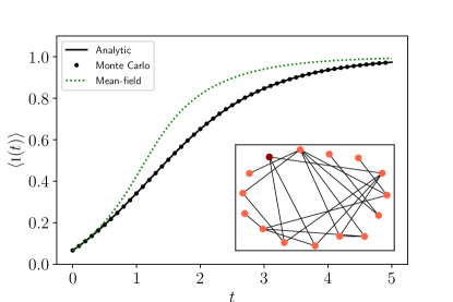
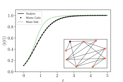
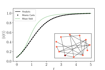
Due to the large number of subgraphs contributing to (40), explicit computation becomes increasingly prohibitive. For this reason, we have created a Python package 333Merbis, Wout; Lodato, Ivano (2021): Exact solutions of the SI model on networks. figshare. Software. https://doi.org/10.6084/m9.figshare.14872182.v3 that, given an input network with specified sources and sinks, computes all contributing subgraphs, their parental relations (54) and the integrals (57) analytically. Here we present explicitly the exact solutions for the prevalence (15) on three small sample networks in figure 2. We suppose that the node marked dark red is a source and compute the expectation values (7) for all of the other nodes. Our algorithm, as detailed in appendix C, computes for each graph all contributing diagrams, finds their parent contributions and constructs the graph of parental relationships. This allows us to integrate (57) starting from the smallest subgraph. The normalized sum over all diagrams with a single sink node gives the prevalence, which we plot as solid black lines in figure 2.
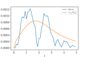
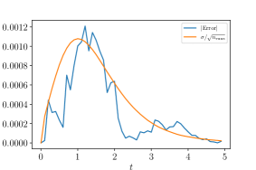
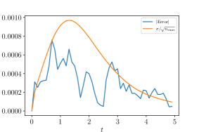
Our analytical results (black line) are in perfect agreement with Monte-Carlo simulations (black dots). These were performed by initializing the networks in the same initial state as in the analytic computation. Then, the Markovian dynamics is simulated by taking small time-steps where susceptible nodes connected to infected nodes are infected with a small infection probability . As this is the only parameter in the model, effectively plays the role of the time-step for a dimensionless time. We choose the value of , small enough to guarantee that at most a single node will flip its state in any one time-step. We simulate spreading trajectories over the same network and record the infection averages. The difference between the simulated average and the analytical formula is of the order of with the standard deviation of the simulated runs, as shown in figure 3. This is a good indication that the averages converge to the exact result in the limit of infinite simulation runs. Note also that analytic and Monte-Carlo results clearly depart from individual-based mean field approximation (green dashed line), which gives an overestimation of the prevalence for finite , as can be seen in figure 2.

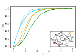
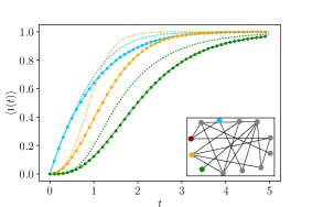
Besides the average expectation value for the full graph, we have also obtained the expectation value for individual nodes in the network. In figure 4 we plot the analytical result (solid line), the Monte-Carlo averages (dots) and the individual based mean-field approximations (dashed line) for three selected nodes in each network. The mean-field approximations are obtained by standard methods (see for instance [7]). The nodes in the network are assumed to be statistically independent, such that at each moment in time. The individual-based mean-field approximation then consists out of the coupled set of ordinary differential equations (ODEs):
| (121) |
Here is the (mean-field) probability of node to be infected at time . This set of equations is easily integrated numerically using a standard ODE integration routine (odeint). The approximation can by improved by including the dynamics for pairs and triples, closing the equations at higher orders [50], though our exact approach captures all correlations present in the network.
VIII Conclusion
In this paper, we have presented a general formalism which allows for obtaining analytic solutions for the expectation values, as well as higher momenta, for the si spreading process on general network. We have decomposed the time-dependent probability vector into a sum over subgraph diagrams, each of which can be computed systematically. We uncovered a set of symmetry relations, which relate contributions from diagrams among each other. Our methods are implemented numerically in [44] and give results which match with Monte-Carlo simulations for several small sample networks of differing topologies.
Even for the relatively small networks analyzed in the previous section, the explicit computation still involves performing thousands of integrals. It is a difficult task to determine exactly how the number of contributing diagrams scales with system size, as this depends strongly on the network topology. In general, the addition of a new edge could potentially double the number of contributing subgraphs, which will then scale exponentially with the number of edges. Using our formalism, one can track only the necessary diagrams contributing to the spreading and systematically organize their contributions by number of edges. In fact, since any diagram with edges will start contributing at the order in the expansion (40), only the smallest contributing subgraphs need be taken into account for an early time estimate of the spreading process. Furthermore, the uncovered symmetry relations and combinations thereof further reduce the number of independent diagrams to be computed. For example, for the three sample networks in figure 2, the number of inequivalent diagrams, including all parents are 9314 (top), 21 376 (center) and 6055 (bottom), out of which only 2274, 1082 and 358 can not be reduced to smaller diagrams using the symmetry relations presented. More symmetry relations may exist, which could further reduce the number of independent diagrams needed to compute the expectations values analytically. For instance, it would be interesting to study relations among contributions of diagrams with double directed edges.
The formalism presented in this letter can be applied to different compartmental models of epidemiology and other out-of-equilibrium stochastic systems on networks [4, 51, 16]. It would be interesting to determine under which conditions exact solutions of such models can be found. We suspect this to be the case for any system where the graph of diagrams is acyclic, such that any diagrams contribution can be traced back to the smallest diagram of a single source.
Appendix A Infinite time limit
We will now prove that the contribution of each diagram reaches asymptotically a constant integer value . As a first step, we explicitly check that the function of for the unique network with edge converges to a constant (integer) value. This is trivial since the expectation value for a one-edge network takes on the form which converges to for . Next we use the inductive hypothesis that all diagrams with edges converge to a non-zero constant for , i.e:
| (122) |
such that and . Now we want to show, using the above hypothesis, that all diagrams with edges converge to a non-zero constant asymptotically. Let us consider the integral
| (123) | ||||
where are all parents of the -edged diagram , which necessarily have edges. Plugging in the inductive hypothesis (122), we get:
| (124) |
where is the multiplicity and relative sign of the -edged parent diagram and denotes the limiting value of that parent. Now we can separate two contributions:
| (125) | ||||
Note that the first term contains a finite contribution when . The second term converges to 0 for . To see this, consider:
| (126) | |||
The asymptotic limit of is evaluated as:
| (127) |
where to obtain the second equality we used L’Hôpital’s rule and in the second line the inductive assumption (122) was used. In addition, , since can only be a constant. Hence we have shown that all diagrams, regardless of the number of edges, will converge asymptotically to a non-zero constant , such that
| (128) |
Next, we prove that is a non-zero integer, i.e. . First, the one-edge diagram has asymptotic value . Let us assume (inductive hypothesis) that all diagrams with single-directed edges have limit . If no double-directed edges are present the number of parents will always be equal to the number of edges going into the blue nodes in the original diagram, . To see this, consider one such diagrams with edges: one can unequivocally obtain its parents by systematically removing one of the edges connecting to one of the sinks. As there are such edges, there will be parents. Finally, the sign of each parent contribution to (128) is equal to the sign of , . This is due to the fact that parents with signs opposing will transition into by one of the rules which induce a sign change. This sign is then contained in and the resulting product will have the same sign as . By induction, then, for the -edged diagram , we have that and hence (128) gives:
| (129) |
If double directed edges exist in a diagram with edges to blue nodes, then there could be more than parents. The reason for this is that each direction on the double directed edge will correspond to different parent diagrams. We can then write down all possible diagrams with the same topology as , but where the double directed edges take on a given orientation, consistent with the graphs source and sink configuration. The number of these diagrams is bounded , since certain double-arrows may exist only conditionally to the existence of other double arrows. Now, each diagram among these will have no double-directed edges and edges to blue nodes, and hence, parents. Each of these parents will have limit by the above argument, so finally:
| (130) |
Hence any diagram will, regardless of its topology, converge to a non-zero integer. This integer corresponds to the number of possible orientations of the double directed edges in the diagram (or equal 1 if there are no double directed edges). For example, the first diagram with a double directed edge (76) converges to , since its sign (75) is negative and there are two possible orientations of the double directed edge (up or down). Each choice of orientation has 2 parents with limit , resulting in a total of 4 parents. The diagram has , such that (128) gives .
Appendix B Proof of (103)
Here we will provide a proof of the ‘cutting off sources’ symmetry relation, presented in section VI.3. For notational convenience, we will use the functions and to denote the diagrams contributions. Here is the graph obtained from by extending the source by one edge. Equation (103) of the main text then reads:
| (131) |
Let us first start by considering , recalling the definition of the contribution as
| (132) |
Here is the number of edges of the diagram . The coefficients count the number of ways the graph can be constructed by applying times on the initial configuration. The difference between the diagrams and is the presence of a chain of length one emanating from the source. Hence to construct the diagram , first the chain must be made, and then the diagram can be created. So for the operator to generate in steps, it must be applied at least once to create the chain, and at most times to create the edges of . The total number of ways to construct is then given by the sum over all ways to construct the chain in steps times the number of ways to construct in steps, such that:
| (133) |
Now, the chain of length one satisfies the recursion relation
| (134) |
with the boundary conditions that . This implies that so that equation (133) becomes
| (135) |
Consider now the sum:
| (136) | |||
or equivalently:
| (137) |
Next, we multiply this equation by and sum over . The right hand side immediately turns into the corresponding contributions as a function of . The left hand side can instead be expressed as the time derivative of :
| (138) | |||
| (139) |
Here we have used the dynamical equation (56) in the main text to obtain the last equality. A simple rewriting now reproduces the equation (131) for a generic graph . One can also obtain a relation between and independent of the parents from solving the differential equation in the first line of (138) as
| (140) |
Appendix C Analytical methods and code
To compute the exact solution for the expectation value in a sample network we developed a numerical code in Python for the integration of each diagram, which combines the network functionality of NetworkX with the symbolic manipulation and integration functionality of SymPy. The algorithm to obtain the exact solution for in (7) consists out of three basic steps. First, we create a list of contributing diagrams as NetworkX DiGraphs by collecting all (labelled) subgraph configurations where the node is blue. Secondly, the graph of diagrams for each inequivalent diagram in the list is constructed by finding the parents of all diagrams, starting from the largest subgraph down to the initial conditions. Grandparents are added iteratively and each diagram is stored as a node in . The multiplicities of topologically inequivalent parents are stored as the edge weights of . Finally, for each diagram in is obtained by integrating eqn. (57). This is done starting from the smallest diagram up to the largest contributing diagram. The result is then the sum over all diagrams contributions obtained in the first step.
The pseudo-code for the algorithm to compute the expectation value is given in Algorithm 1. It relies on a number of functions which we will expand upon below. computes a list of all labelled subgraph configurations which contribute to the expectation value for the node to be infected at time , given that node was initially infected. gives a list of parent diagrams which transition into diagram by applying the dynamical rules of the si system. simply computes the sign (75) of a diagram and is needed if the dynamical rules generate a sign difference between the parent and the child diagram, for instance by closing a loop on a blue node.
C.1 Contributing diagrams
The list of contributing diagrams is constructed as follows. First, the graph is initialized by defining the states of the source node and the sink node . Then all possible paths from to are stored in a list and a directed diagram is built from these paths, with only white nodes in between and . The resulting diagram is an acyclic directed graph containing all possible paths from to corresponding to the largest possible diagram contributing to the expectation value. From this diagram, edges are removed systematically such that the resulting graph is connected and all remaining nodes stay within the in-component of the blue node . If any node is not in the in-component of the node , it is removed along with all edges connected to it. Each resulting connected diagram is added to the list of contributing diagrams. The pseudo-code for this algorithm is provided in Algorithm 2.
C.2 The Get Parents function
In order to integrate any give diagram, one needs to recover the parents of that diagram. This can be done by tracing the rules of the si model backwards. The parents of any given diagram necessarily have one edge less connected to a blue node. They can thus be obtained by systematically removing single edges connected to the sinks, while leaving all other edges intact. However, the neighbor connected to the removed edge might change state from white to blue, as the forward action of can project blue nodes into white ones. Special care must be made to include only actual parents in the list of parent diagrams, as some coloring of nodes can not be obtained from the forward action of on the initial conditions. For instance, it is impossible to have a diagram with two neighboring blue nodes (connected by an edge). Similarly, it is not possible to have a branch in the diagram without a blue node, as there would be no path from source to sink in that branch.
To determine whether a candidate parent of a given diagram can actually exist, we exploit the directed edges representing the flow from sources to sinks. Specifically, we must check that for each neighbor of a sink, after removal of their edge, other outgoing edges from exist. If so, the node cannot be blue and must be white (sinks cannot have outgoing edges). If, on the other hand, the neighboring node has only incoming edges, it must be turned blue, since the flow of information must end in a sink. Finally, there is a scenario where the node can be both blue or white. This happens when the node has only double directed edges as outgoing edges, and so the set of out-neighbors of is contained within the set of in-neighbors . In that case, both the diagrams with node white and blue are valid parents. It could also be that some paths are no longer possible after removing the edge to a blue node, or after turning a white node blue. Therefore, the direction of the edges for the parent diagrams should be re-evaluated in each case. The pseudo-code for the algorithm which constructs all physical parents of any arbitrary diagram is given in Algorithm 3.
Our code is freely available in the online public repository [49], along with a list of contributions for all diagrams with up to 10 edges. The repository also includes several Jupyter notebooks where the example graphs of the main text are computed using our algorithms. These notebooks contain the exact analytical expressions for the infection prevalence plotted in Fig. 2 of the main text.
Appendix D Explicit functions for the first few diagrams
For completeness we list here the explicit functions corresponding to all diagrams with up to four edges.
Acknowledgements.
WM wishes to thank Clelia de Mulatier for useful discussions and acknowledges the support from the NWO Klein grant awarded to NWA route 2 in 2020.References
- Anderson and May [1992] R. M. Anderson and R. M. May, Infectious diseases of humans (Oxford University Press, Oxford, 1992).
- Strogatz [2001] S. H. Strogatz, Exploring complex networks, nature 410, 268 (2001).
- Albert and Barabási [2002] R. Albert and A.-L. Barabási, Statistical mechanics of complex networks, Reviews of modern physics 74, 47 (2002).
- Boccaletti et al. [2006] S. Boccaletti, V. Latora, Y. Moreno, M. Chavez, and D.-U. Hwang, Complex networks: Structure and dynamics, Physics reports 424, 175–308 (2006).
- Barrat et al. [2008] A. Barrat, M. Barthelemy, and A. Vespignani, Dynamical processes on complex networks (Cambridge university press, 2008).
- Castellano et al. [2009] C. Castellano, S. Fortunato, and V. Loreto, Statistical physics of social dynamics, Reviews of modern physics 81, 591 (2009).
- Newman [2018] M. Newman, Networks (Oxford university press, 2018).
- Carletti et al. [2020] T. Carletti, D. Fanelli, and F. Piazza, Covid-19: The unreasonable effectiveness of simple models, Chaos, Solitons & Fractals: X 5, 100034 (2020).
- Nielsen et al. [2021] B. F. Nielsen, L. Simonsen, and K. Sneppen, Covid-19 superspreading suggests mitigation by social network modulation, Physical Review Letters 126, 118301 (2021).
- Moein et al. [2021] S. Moein, N. Nickaeen, A. Roointan, N. Borhani, Z. Heidary, S. H. Javanmard, J. Ghaisari, and Y. Gheisari, Inefficiency of sir models in forecasting covid-19 epidemic: a case study of isfahan, Scientific Reports 11, 1 (2021).
- Kermack and McKendrick [1927] W. O. Kermack and A. G. McKendrick, A contribution to the mathematical theory of epidemics, Proceedings of the Royal Society A, 700–721 (1927).
- Brauer [2008] F. Brauer, Compartmental models in epidemiology (2008).
- Keeling and Rohani [2011] M. J. Keeling and P. Rohani, Modeling infectious diseases in humans and animals (Princeton university press, 2011).
- Pastor-Satorras and Vespignani [2001] R. Pastor-Satorras and A. Vespignani, Epidemic spreading in scale-free networks, Physical review letters 86, 3200 (2001).
- Newman [2002] M. E. J. Newman, Spread of epidemic disease on networks, Physical review E, 016128 (2002).
- Pastor-Satorras et al. [2015] R. Pastor-Satorras, C. Castellano, P. Van Mieghem, and A. Vespignani, Epidemic processes in complex networks, Reviews of modern physics 87, 925 (2015).
- Khan et al. [2009] H. Khan, R. N. Mohapatra, K. Vajravelu, and S. Liao, The explicit series solution of sir and sis epidemic models, Applied Mathematics and Computation 215, 653 (2009).
- Harko et al. [2014] T. Harko, F. S. Lobo, and M. Mak, Exact analytical solutions of the susceptible-infected-recovered (sir) epidemic model and of the sir model with equal death and birth rates, Applied Mathematics and Computation 236, 184 (2014).
- Bohner et al. [2019] M. Bohner, S. Streipert, and D. F. Torres, Exact solution to a dynamic sir model, Nonlinear Analysis: Hybrid Systems 32, 228 (2019).
- Kozyreff [2021] G. Kozyreff, Near-exact explicit asymptotic solution of the sir model well above the epidemic threshold, medRxiv (2021).
- May and Lloyd [2001] R. M. May and A. L. Lloyd, Infection dynamics on scale-free networks, Physical Review E 64, 066112 (2001).
- Pastor-Satorras and Vespignani [2002] R. Pastor-Satorras and A. Vespignani, Epidemic dynamics in finite size scale-free networks, Physical Review E 65, 035108 (2002).
- Eguiluz and Klemm [2002] V. M. Eguiluz and K. Klemm, Epidemic threshold in structured scale-free networks, Physical Review Letters 89, 108701 (2002).
- Boguná et al. [2003] M. Boguná, R. Pastor-Satorras, and A. Vespignani, Absence of epidemic threshold in scale-free networks with degree correlations, Physical review letters 90, 028701 (2003).
- Van Mieghem et al. [2008] P. Van Mieghem, J. Omic, and R. Kooij, Virus spread in networks, IEEE/ACM Transactions On Networking 17, 1–14 (2008).
- Castellano and Pastor-Satorras [2010] C. Castellano and R. Pastor-Satorras, Thresholds for epidemic spreading in networks, Physical review letters 105, 218701 (2010).
- Van Mieghem [2011] P. Van Mieghem, The n-intertwined sis epidemic network model, Computing 93, 147 (2011).
- Cai et al. [2016] C.-R. Cai, Z.-X. Wu, M. Z. Chen, P. Holme, and J.-Y. Guan, Solving the dynamic correlation problem of the susceptible-infected-susceptible model on networks, Physical review letters 116, 258301 (2016).
- Wang et al. [2017] W. Wang, M. Tang, H. E. Stanley, and L. A. Braunstein, Unification of theoretical approaches for epidemic spreading on complex networks, Reports on Progress in Physics 80, 036603 (2017).
- Harding et al. [2018] N. Harding, R. Nigmatullin, and M. Prokopenko, Thermodynamic efficiency of contagions: a statistical mechanical analysis of the sis epidemic model, Interface focus 8, 20180036 (2018).
- Matamalas et al. [2018] J. T. Matamalas, A. Arenas, and S. Gómez, Effective approach to epidemic containment using link equations in complex networks, Science advances 4, eaau4212 (2018).
- Wang et al. [2019] W. Wang, Q.-H. Liu, J. Liang, Y. Hu, and T. Zhou, Coevolution spreading in complex networks, Physics Reports 820, 1 (2019).
- Simon et al. [2011] P. L. Simon, M. Taylor, and I. Z. Kiss, Exact epidemic models on graphs using graph-automorphism driven lumping, Journal of mathematical biology 62, 479–508 (2011).
- Kiss et al. [2015] I. Z. Kiss, C. G. Morris, F. Sélley, P. L. Simon, and R. R. Wilkinson, Exact deterministic representation of markovian sir epidemics on networks with and without loops, Journal of mathematical biology 70, 437–464 (2015).
- Cator and Van Mieghem [2013] E. Cator and P. Van Mieghem, Susceptible-infected-susceptible epidemics on the complete graph and the star graph: Exact analysis, Physical Review E 87, 012811 (2013).
- Prasse and Van Mieghem [2020] B. Prasse and P. Van Mieghem, Time-dependent solution of the nimfa equations around the epidemic threshold, Journal of Mathematical Biology 81, 1299 (2020).
- Demongeot et al. [2020] J. Demongeot, Q. Griette, and P. Magal, Si epidemic model applied to covid-19 data in mainland china, Royal Society open science 7, 201878 (2020).
- Moore and Rogers [2020] S. Moore and T. Rogers, Predicting the speed of epidemics spreading in networks, Physical review letters 124, 068301 (2020).
- Verhulst [1838] P.-F. Verhulst, Notice sur la loi que la population suit dans son accroissement, Correspondance mathématique et physique 10, 113–121 (1838).
- Merbis [2021] W. Merbis, Exact epidemic models from a tensor product formulation, arXiv:2102.11708 (2021).
- Note [1] We use a bra-ket notation for column vectors and row vectors , such that their contraction is denoted as .
- Gaspard [2005] P. Gaspard, Chaos, scattering and statistical mechanics, 9 (Cambridge University Press, 2005).
- Lecomte et al. [2007] V. Lecomte, C. Appert-Rolland, and F. Van Wijland, Thermodynamic formalism for systems with markov dynamics, Journal of statistical physics 127, 51 (2007).
- Note [2] We assume the underlying network topology has only undirected edges, such that .
- Breiger and Pattison [1986] R. L. Breiger and P. E. Pattison, Cumulated social roles: The duality of persons and their algebras, Social networks 8, 215 (1986).
- Newman and Watts [1999] M. E. Newman and D. J. Watts, Renormalization group analysis of the small-world network model, Physics Letters A 263, 341 (1999).
- Watts and Strogatz [1998] D. J. Watts and S. H. Strogatz, Collective dynamics of ‘small-world’networks, nature 393, 440–442 (1998).
- Erdös et al. [1960] P. Erdös, A. Rényi, et al., On the evolution of random graphs, Publ. Math. Inst. Hung. Acad. Sci 5, 17 (1960).
- Note [3] Merbis, Wout; Lodato, Ivano (2021): Exact solutions of the SI model on networks. figshare. Software. https://doi.org/10.6084/m9.figshare.14872182.v3.
- Kiss et al. [2017] I. Z. Kiss, J. C. Miller, P. L. Simon, et al., Mathematics of epidemics on networks, Vol. 598 (Springer, 2017).
- Gleeson [2013] J. P. Gleeson, Binary-state dynamics on complex networks: Pair approximation and beyond, Physical Review X 3, 021004 (2013).