Long-term multi-band photometric monitoring of Mrk 501

Abstract

Aims. Radio-to-TeV observations of the bright nearby (z=0.034) blazar Markarian 501 (Mrk 501), performed from December 2012 to April 2018, are used to study the emission mechanisms in its relativistic jet.

Methods. We examined the multi-wavelength variability and the correlations of the light curves obtained by eight different instruments, including the First G-APD Cherenkov Telescope (FACT), observing Mrk 501 in very high-energy (VHE) gamma-rays at TeV energies. We identified individual TeV and X-ray flares and found a sub-day lag between variability in these two bands.

Results. Simultaneous TeV and X-ray variations with almost zero lag are consistent with synchrotron self-Compton (SSC) emission, where TeV photons are produced through inverse Compton scattering. The characteristic time interval of 5-25 days between TeV flares is consistent with them being driven by Lense-Thirring precession.

1 Introduction

Blazars are active galactic nuclei (AGN) with a relativistic jet pointed towards the observer. These sources emit from the radio to the TeVs, and they are the most populous group of objects detected above 100 GeV. Their emission is non-thermal and is typically characterised by two broad bumps peaking in the infrared to the X-rays, and in the $\gamma$-rays. The low-energy bump is associated with synchrotron radiation of relativistic electrons. Depending on the peak energy of this component, blazars can be subdivided into low (peaking in the infrared), intermediate, or high (peaking in the X-rays) synchrotron-peaked blazars (LBL, IBL, and HBL respectively). Multi-wavelength variability studies provide important insight into the jet inner structure and emission mechanisms. In addition to the electromagnetic radiation, neutrinos have also been associated with some blazars and were used to probe the radiation processes within the jet (Mücke & Protheroe, 2001a, b; Petropoulou et al., 2016; Mannheim, 1993).

Markarian 501 (Mrk 501) is one of the most frequently studied nearby ($z=0.034$) bright blazars and was discovered to be a TeV source by the Whipple imaging atmospheric Cherenkov telescope (Quinn et al., 1996). Mrk 501 has been monitored extensively in the radio (Richards et al., 2011; Piner et al., 2010), V-band (Smith et al., 2009), X-rays (MAGIC Collaboration et al., 2020; Abdo et al., 2011b), and $\gamma$-rays (Abdo et al., 2011b; Dorner et al., 2015; Abeysekara et al., 2017; Ahnen et al., 2017). Although variability is present in all energy bands, it peaks in the TeV, with a flux varying from 0.3 to 10 times that of the Crab nebula (Crab Unit, CU) (Aharonian et al., 1999). In 2012, Mrk 501 was simultaneously observed by 25 different instruments during a three-month campaign (Ahnen et al., 2018) and was found in an intermediate state with a TeV flux of about 0.5 CU that reached 4.9 CU on June 9. The TeV outburst was also accompanied by X-ray flares that were detected by Swift/XRT. This campaign reported the hardest VHE spectra ever measured, with a power-law index close to 2. The bumps in spectral energy distribution (SED) peaked at above 5 keV and 0.4 TeV, respectively, indicating that the source is an extreme HBL (EHBL). This extreme spectrum could be transient, the usual harder-when-brighter TeV spectrum was not observed either, in contrast to previous multi-wavelength campaigns (Acciari et al., 2011b; Aharonian et al., 2001; Albert et al., 2007b; Abdo et al., 2011a).

A one-zone SSC model reasonably explains the overall shape of the SED (Bartoli et al., 2012; Aleksić et al., 2015a; Ahnen et al., 2018) and accounts for most of its emission. Mismatches were pointed out during some flares (e.g. Ahnen et al., 2018, 2017), and were sometimes solved using two different emitting zones (Bartoli et al., 2012; Ahnen et al., 2018) or hadronic processes (Sahu et al., 2020b; Shukla et al., 2015). For example, the flare on June 9, 2012, could not be explained using a one-zone SSC model (Ahnen et al., 2018), and a second smaller emission zone, mostly contributing to the X-rays and TeVs, was added. The acceleration mechanism in the SSC framework is also unclear, with authors claiming magnetic reconnections (Ahnen et al. (2018)) or Fermi first-order acceleration (Shukla et al., 2015). Another approach is to consider a photo-hadronic model (Sahu et al., 2020b; Shukla et al., 2015), where Fermi-accelerated protons produce the VHE $\gamma$-rays through the photo-pion process. As the most significant gamma-ray variations occur during the high state of Mrk 501 (Abdo et al., 2011c; Zech et al., 2017), comparing models applied to different source states is also difficult.

In this paper, we report observations that took place between 2012 and 2018 from the radio to the TeV, which were part of a long-term multi-wavelength campaign carried out with the FACT telescope. This paper is structured as follows. In Sect. 2 we briefly describe the instruments and data reduction techniques we used to obtain the light curves. In Sect. 3 we report the investigations of the variability, auto- and cross-correlations of the light curves, identification and correlations of individual TeV and X-ray flares, and analysis of the correlations between GeV and radio variations. Section 4 includes the discussion of the main results, with an emphasis on the likely underlying physical processes. Finally, Sect. 5 provides a summary of the results and conclusions.

2 Data and analysis

To characterise the long-term variability of Mrk 501, we gathered data taken between December 14, 2012, and April 18, 2018, with eight different instruments observing from the radio to the TeV. The instruments and data reduction techniques are described in the following subsections, and the resulting light curves are presented in Fig. 1. The light curves obtained for FACT and Swift/BAT include negative count rates, as expected when the emission from a source is lower than the sensitivity of a background-dominated instrument.

The Fermi-LAT light curve is always positive because of the use of a positively defined model in the maximum likelihood fitting. Correlations and variability analyses presented in Sect. 3 disregard negative or low signal-to-noise ratio (¡2 sigma) data points. Flare identification used complete light curves because uncertainties are properly considered in the Bayesian Block algorithm.

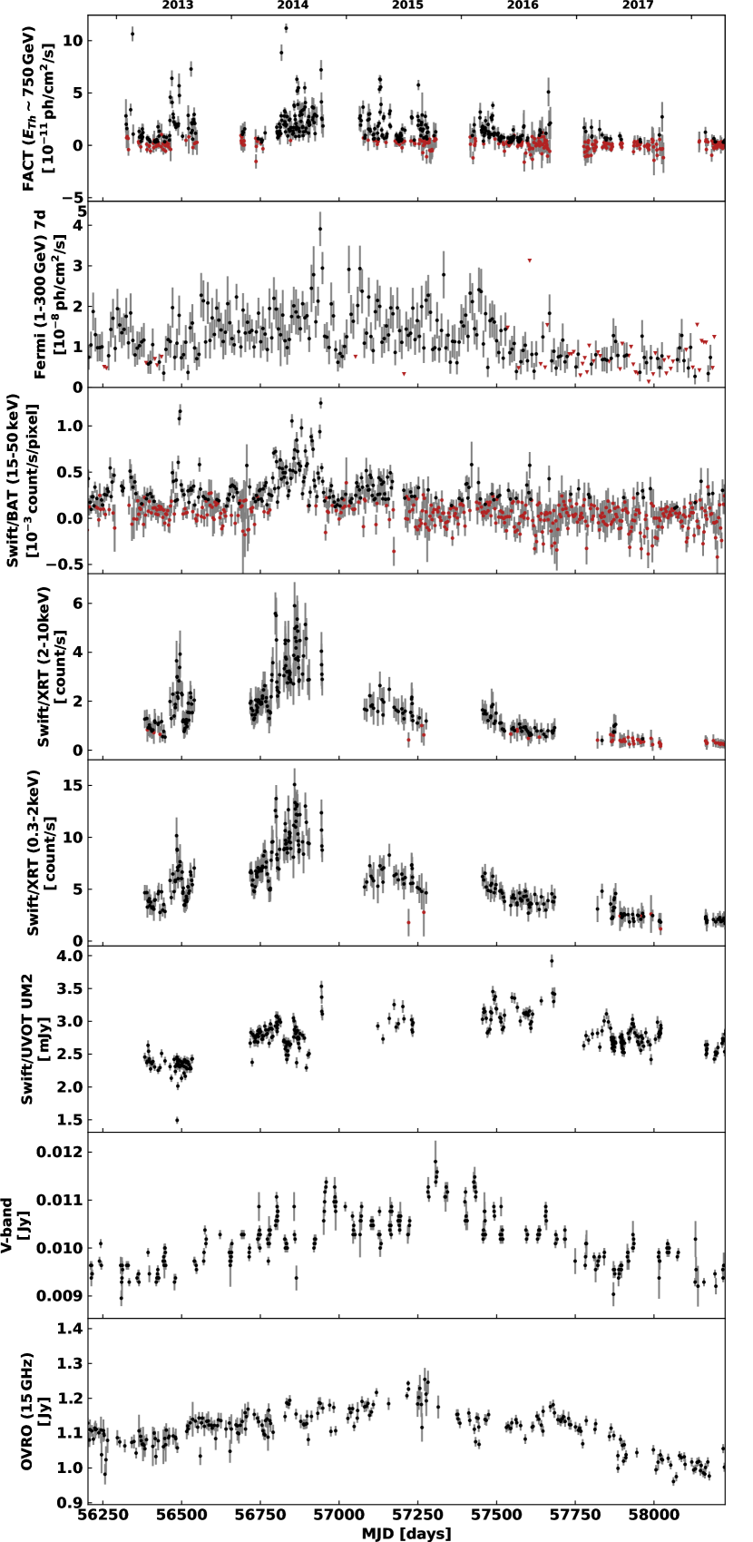
Figure 1: Long-term light curves of Mrk 501 obtained from the radio to the TeVs between December 14, 2012, and April 18, 2018. From top to bottom: FACT ($E_{Th}$ $\sim$750 GeV) nightly binning, Fermi-LAT (1-300 GeV) one-week binning, Swift/BAT (15-50 keV) two-day binning, Swift/XRT (2-10 keV), Swift/XRT (0.3-2 keV), and UM2 Swift/UVOT V-band optical observations, and radio observations at 15 GHz. Flux measurement errors are denoted as vertical grey bars. Points with a signal-to-noise ratio lower than 2 are plotted in red (see Sect. 2 for details about the cleaning procedures). For the Fermi-LAT light curve, the 95% flux upper limits (TS¡25) are shown with triangles.

2.1 Radio to GeV observations

Mrk 501 was observed by Owens Valley Radio Observatory (OVRO) 40 meters telescope as part of the Fermi-LAT high-cadence blazars monitoring program (Richards et al., 2011). The radio receiver of the OVRO telescope has a centre frequency of 15 GHz with a 3 GHz bandwidth and an aperture efficiency $\sim 0.25$. The radio flux densities were obtained using ON-ON technique for dual-beam optics configuration to minimise ground and atmospheric contamination of the signal. The noise at the level of 55 K, which includes actual thermal noise of 30 K, the CMB, as well as atmospheric and ground contributions, leads to a $\sim 5\%$ systematic flux uncertainty. Observations were mostly performed twice per week. The data were publicly available online from the Owens Valley Radio Observatory archive. A complete description of the instrument, calibrations, and analysis is provided in Richards et al. (2011).

Regular observations of Mrk 501 were performed in the V-band as part of the optical monitoring of $\gamma$-ray blazars to support Fermi-LAT observations by the 1.54 m Kuiper and 2.3 m Bok telescopes at Steward Observatory (Smith et al., 2009). All the data are publicly available, and for the time period used in this paper, we used data from Cycle 5 to Cycle 10, spanning from September 9, 2012, until March 2018 .

Mrk 501 observations in three ultraviolet bands (W1, M2, and W2 filters) are available from the Swift Ultra-Violet and Optical Telescope (UVOT) (Roming et al., 2005). Standard aperture photometry analysis was performed using the Swift/UVOT software tools from the HEASOFT package (version 6.24). Calibration data were obtained from the CALDB (version 20170922). An aperture of 6 arcsec radius was used for the flux extraction for all the filters. The background flux level was estimated in an annulus with radii 11 or 19 arcsec centred on the location of Mrk 501. The two regions we used for source and background estimation were verified to not include light from any nearby sources, stray light, or elements of UVOT supporting structures. Dereddening of the fluxed was performed following the prescription from Roming et al. (2009) using $E(B-V)=0.0164$ (Schlafly & Finkbeiner, 2011).

Observations in the X-rays (0.2-10 keV) were performed by the Swift/XRT X-ray telescope (Burrows et al., 2005). Considering the SED of Mrk 501, the X-ray light curves from Swift/XRT were built for the 0.3-2 keV and 2-10 keV bands separately to probe the emission process below and above the cutoff energy. Swift/XRT performed regular high-quality observations of Mrk 501. The light curve is publicly available using the Swift-XRT products generation tool . This tool uses HEASOFT software version 6.22, and the complete analysis pipeline is described in Evans et al. (2009).

The Burst Alert Telescope (BAT, Krimm et al., 2013) on board of the Swift satellite allows monitoring the complete sky at hard X-rays every few hours. The Swift/BAT reduction pipeline is described in Tueller et al. (2010) and Baumgartner et al. (2013). Our pipeline is based on the BAT analysis software HEASOFT version 6.13. A first analysis was performed to derive background detector images. We created sky images (task batsurvey) in the eight standard energy bands (in keV: 14 - 20, 20 - 24, 24 - 35, 35 - 50, 50 - 75, 75 - 100, 100 - 150, and 150 - 195) using an input catalogue of 86 bright sources that have the potential of being detected in single pointings. The detector images were then cleaned by removing the contribution of all detected sources (task batclean) and averaged to obtain one background image per day. The variability of the background detector images was smoothed pixel by pixel, fitting the daily background values with a polynomial model. The BAT image analysis was then run using these smoothed averaged background maps. The result of our processing was compared to the standard results presented by the Swift team (light curves and spectra of bright sources from the Swift/BAT 70-month survey catalogue), and a very good agreement was found. The Swift/BAT light curves of Mrk 501 were built in several energy bands. For each time bin and energy band, a weighted mosaic of the selected data was first produced, and the source region count rate was extracted assuming a fixed source position and shape of the point spread function. The signal-to-noise ratio of the source varies regularly because of intrinsic variability, its position in the BAT field of view, and the distance to the Sun. The 15-50 keV two-day bin light curve presented in Fig. 1 spans from December 14, 2012, to April 18, 2018, that is, over 29344 orbital periods or almost 5.5 years.

The Large Area Telescope on board the Fermi Gamma-ray Space Telescope (hereafter Fermi-LAT) is a $\gamma$-ray detector that is sensitive from 20 MeV to 300 GeV (Atwood et al., 2009; Abdo et al., 2009; Ackermann et al., 2012a, b). Data are publicly available and have been analysed with the Fermitools.

We performed a binned analysis following the Fermi-LAT team recommendations. We used only photons with energy between 1 GeV and 300 GeV within a square of $21^{\circ}\times 21^{\circ}$ centred on Mrk 501, flagged with evclass=128 and evtype=3, and with a maximum zenith angle of $90^{\circ}$. Data were processed with the PASS8, using the P8R3_SOURCE_V2 instrument response function. To model the region surrounding Mrk 501, we used the sources in the 4FGL catalogue (Abdollahi et al., 2020), up to $5^{\circ}$ outside the box, and we described the Galactic diffuse emission and the isotropic extra-Galactic component with gll_iem_v07 and iso_P8R3_SOURCE_V2_v1, respectively. The best fit over the entire time data sample, describing Mrk 501 with a log-parabola model $dN/dE=N(E/E_{\rm b})^{-\alpha+\beta(Log(E/E_{b}))}$ , yielded $N=(4.07\pm 0.06)\times 10^{-12}$ $\rm cm^{-2}\leavevmode\nobreak\ s^{-1}\leavevmode\nobreak\ MeV^{-1}$, $\alpha=1.73\pm 0.01$, $\beta=0.013\pm 0.005$, with $E_{\rm b}=1476.73$  MeV. The same fit also yielded a normalisation of $0.97\pm 0.01$ for the Galactic diffuse emission and $0.97\pm 0.01$ for the isotropic one. We also verified that there were no significant residuals from the whole time test-statistic map.

To obtain the light curve, we fitted the model in each time bin (3, 7, and 30 days), keeping the Galactic diffuse and the extragalactic isotropic normalisations fixed to their average values, and freeing the normalisation of the brightest sources within $8^{\circ}$ from the centre and with more than ten predicted photons. When Mrk 501 was detected with a TS¡25, we calculated 95% flux upper limits. The distribution of the $\alpha$ parameter and the integrated flux for Mrk 501 varied by less than $0.3\%$ and $1\%$, respectively, when we let the Galactic and extragalactic normalisation parameters free in the fit. If instead we freed more sources, $\alpha$ and the integrated flux might vary up to $3\%$ and $10\%$, respectively.

2.2 TeV observations by FACT

The First G-APD Cherenkov Telescope (FACT) is located in the Observatorio del Roque de los Muchachos on the island La Palma at 2.2 km a.s.l. (Anderhub et al., 2013). Using the imaging air Cherenkov technique, it has been operational since October 2011. With its 9.5 m² segmented mirror, FACT detects gamma-rays with energies above a few hundred GeV by observing the Cherenkov light produced in extensive air showers induced by gamma and cosmic rays in the Earth’s atmosphere. This approach allows for consistent long-term unbiased monitoring at TeV energies. Typically, no human interaction is needed during the night. The shift is performed fully remote and in an automatic way by software. In combination with an unbiased observing strategy, this allows for consistent long-term monitoring at TeV energies. This is facilitated by the excellent and stable performance of the camera using silicon-based photosensors (SiPM, also known as Geiger-mode avalance photo diods; G-APDs) and a feedback system, keeping the gain of the photosensors stable (Biland et al., 2014). On the one hand, the stable and automatic operation maximises the data-taking efficiency, and with this, the duty cycle of the instrument. On the other hand, the usage of SiPMs also minimises the gaps in the light curves (Dorner et al., 2017) as these photosensors allow for observations with bright ambient light. While the telescope can operate during full-Moon conditions (Knoetig et al., 2013), observations are typically interrupted for 4-5 days every month for safety reasons associated with the operational conditions at the observatory site.

Between December 14, 2012, and April 18, 2018, a total of 1953 hours of physics data from Mrk 501 have been collected during 889 nights with up to 5.5 hours per night and an average nightly observation time of 2.2 hours. To ensure enough event statistics, nights with an observation time of less than 20 minutes were removed from the data sample. After this and after data quality selection (see below), 1344 hours from 633 nights remain. The FACT light curve is shown in Fig. 1 (uppermost panel).

To derive the light curve, the data were processed using the modular analysis and reconstruction software (MARS, revision 19203; Bretz & Dorner, 2010). The feedback system enables stable and homogeneous gain that does not need to be recalibrated. After signal extraction, the images were cleaned using a two-step process, as described in Arbet-Engels et al. (2021). Based on a principal component analysis of the remaining distribution, a set of parameters describing the shower image was obtained. A detailed description of the image reconstruction and background suppression cuts for light curve and spectral extraction is provided in Beck et al. (2019). By cutting in the angular distance between the reconstructed source position and the real source position in the camera plane, $\theta$, (at $\theta^{2}<0.037$ deg²), the signal from the source was determined. To estimate the background, the same cut was applied for five off-source regions, each located 0.6 deg from the camera centre (observations are typically carried out in wobble-mode (Fomin et al., 1994) with a distance of 0.6 deg from the camera centre).

The excess rate was calculated by subtracting the scaled signal in these off-regions from the signal at the source position and dividing it by the effective exposure time. To study and correct the effect of the zenith distance and trigger threshold (changing with ambient light conditions) (Bretz et al., 2013), the excess rate of the Crab nebula was used. While flares in the MeV/GeV range have been seen, similar flux changes have not been found at TeV energies. Therefore the Crab nebula was used as a standard candle at TeV energies. The dependences of the excess rate on observing conditions are similar to those of the cosmic-ray rate described in Bretz (2019), and details can be found in Beck et al. (2019).

For the studied data sample, the corrections in zenith distance are smaller than 10% for more than 97% of the nights, and in trigger threshold, lower than 10% for more than 75% of the nights. The maximum correction in zenith distance is 44%, and only two nights need a correction larger than 40%. In threshold, the largest correction is 72%, but 99% of the nights have a correction smaller than 60%.

To verify the effect of the different spectral slopes of Mrk 501, the spectra of 35 time ranges between February 2013 and August 2018 determined using the Bayesian Block algorithm (see Sect. 3) were extracted (see details in Temme et al. (2015) and background suppression cuts from Beck et al. (2019)) were fitted with a simple power law. Within the uncertainties, no obvious correlation was found between index and flux, so that the harder-when-brighter behaviour reported in Aleksić et al. (2015b) is not confirmed for the TeV energy band. The distribution of indices yields an average spectral slope of $2.96\pm 0.26$, which is compatible with some previously published results of other telescopes, taking the different energy ranges and instrument systematics into account (Albert et al., 2007a). Assuming different slopes from $2.7$ to $3.22$, the corresponding energy thresholds ($E_{Th}\sim 750\,GeV$ (Cologna et al., 2017)) and integral fluxes were determined to estimate the systematic error of a varying slope of the spectrum of Mrk 501. This resulted in a systematic flux uncertainty lower than 7%, which was added quadratically to the statistical uncertainties.

For the light curve of Mrk 501, a data quality selection cut based on the cosmic-ray rate (Hildebrand et al., 2017) was applied to the data sample from December 14, 2012, until April 18, 2018 (MJD 56275 to 58226). For this, the artificial trigger rate $R750$ was calculated above a threshold of 750 DAC-counts, which was found to be independent of the actual trigger threshold. The remaining dependence of $R750$ on the zenith distance was determined (as described in (Mahlke et al., 2017) and (Bretz, 2019)). A corrected rate $R750_{\rm cor}$ was calculated based on this. Seasonal changes of the cosmic-ray rate due to variations in the Earth’s atmosphere were taken into account by determining a reference value $R750_{\rm ref}$ for each moon period. The distribution of the ratio $R750_{\rm cor}$/$R750_{\rm ref}$ can be described with a Gaussian distribution for the good-quality data, while data with poo quality lies outside the Gaussian distribution. A cut was applied at the points at which the distribution of all data starts to deviate from the Gaussian distribution. Therefore, data with good quality were selected using a cut of $0.93<R750_{\rm cor}/R750_{\rm ref}<1.3$ (Arbet-Engels et al., 2021). This resulted in a total of 1344 hours of good-quality data from Mrk 501 during the discussed time period, distributed over 633 nights, as shown in Fig. 1 (uppermost panel).

3 Timing analysis

In this section, we investigate the variability of Mrk 501 band by band using fractional variability and auto-correlation functions. We also use Bayesian Block analysis to identify individual flares and distinguish different source states. Temporal relations between different spectral bands are probed using cross-correlation functions and convolution techniques.

3.1 Variability

The variability in light curves can be compared and quantified by the unit-less fractional variability $F_{var}=\sqrt{(S^{2}-\langle\sigma^{2}_{err}\rangle)/\langle{x}\rangle^{2}}$ (Vaughan et al., 2003), where S is the standard deviation of the light curve, $\langle\sigma^{2}_{err}\rangle$ is the mean squared flux error, and $\langle{x}^{2}\rangle$ is the square of the average flux. Uncertainties of the fractional variability were estimated using the prescription by Poutanen et al. (2008) and Vaughan et al. (2003).

The dependence of the fractional variability on frequency, calculated for the light curves spanning about 5.5 years, is depicted in Fig. 2. The fractional variability is lowest in the radio and optical, increases up to the X-rays, drops in the GeV, and again increases up to the TeV, where the highest variability is found. These two maxima indicate that the falling edges of the two SED components are more variable than the rising ones and that the component peaking in the TeV varies more than the component peaking in the X-rays. Similar behaviour was observed in Mrk 421 (Aleksić et al., 2015b, c; Arbet-Engels et al., 2021). Some previous studies of Mrk 501 focusing on the study of large flares found a fractional variability that monotonically increased with frequency (Aliu et al., 2016; Ahnen et al., 2017). Different binning, cadence, and coverage in the different wavebands may play a role in this discrepancy (Schleicher et al., 2019).

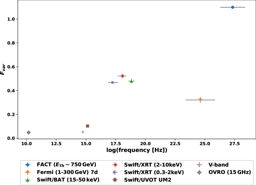
Figure 2: Fractional variability $F_{var}$ as a function of frequency. X-axis error bars indicate the energy band of the instrument. Y-axis error bars denote the uncertainty of $F_{var}$ , which for some instruments are smaller than the marker.

We calculated the structure functions (SF, Simonetti et al., 1985) of the various light curves and found in the X-rays an average SF slope of 0.13 and first break at around 20 days. In the TeV range, the average slope of the SF is 0.09. In the radio, the SF slope is close to zero, suggesting either white noise rather than well-structured flares or numerous overlapping flares.

3.2 Light-curve correlations

We correlated the light curves either with themselves (auto-correlation) or with other light curves using the discrete correlation function (DCF, Edelson & Krolik, 1988), which properly takes the irregular sampling of the data into account. All the correlations were calculated by filtering out the data of low significance (¡$2\sigma$) and additionally discarding all upper limits from the Fermi-LAT light curve, as is often done in the literature (e.g. Acciari et al., 2011a; Ahnen et al., 2018). The uncertainties were calculated with the DCF algorithm.

A time bin of one day was used in the discrete auto-correlation function (DACF) for most data, except in the UV, optical, and radio (three days) and in the GeV. As the Fermi-LAT flux uncertainties are correlated because the same sky model was used for the different time bins, we had to use a time bin of 20 days (see the discussion in Edelson & Krolik, 1988). Shorter lags would result in a correlation above unity (see the grey curve in Fig. 3). For the TeV and X-rays cross-correlations, we used a one-day lag binning, while for the radio and optical correlations with GeV, we used three days.

The auto-correlations (Fig. 3) indicate the presence of flares developing on a timescale of a few days mostly in the TeV and hard X-rays and of variations occurring on timescales of many weeks. As the shortest variability timescale of Mrk 501 in the X-rays ($\sim$one day, Tanihata et al., 2001) is shorter than our time bins, the correlation peaks characterise flaring patterns longer than the binning period.

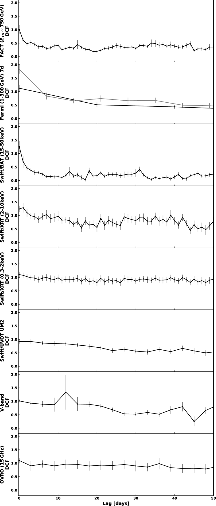
Figure 3: Light-curve auto-correlations. From top to bottom: FACT, Swift/BAT, Swift/XRT (2-10 keV), Swift/XRT (0.3-2 keV), Fermi-LAT, Swift/UVOT UM2, V-band, and radio. Grey error bars denote 1$\sigma$ DCF uncertainties. A one-day binning was used, except for Fermi-LAT (20- and 7-day lag binning, black and grey lines, respectively) and for the UV, optical, and radio data (3 days).

We tested the cross-correlations between all light curves and discuss the significant ones (TeV/X-rays, UV/V-band, and GeV/radio) in Sect. 3.3, 3.4, and 3.5.

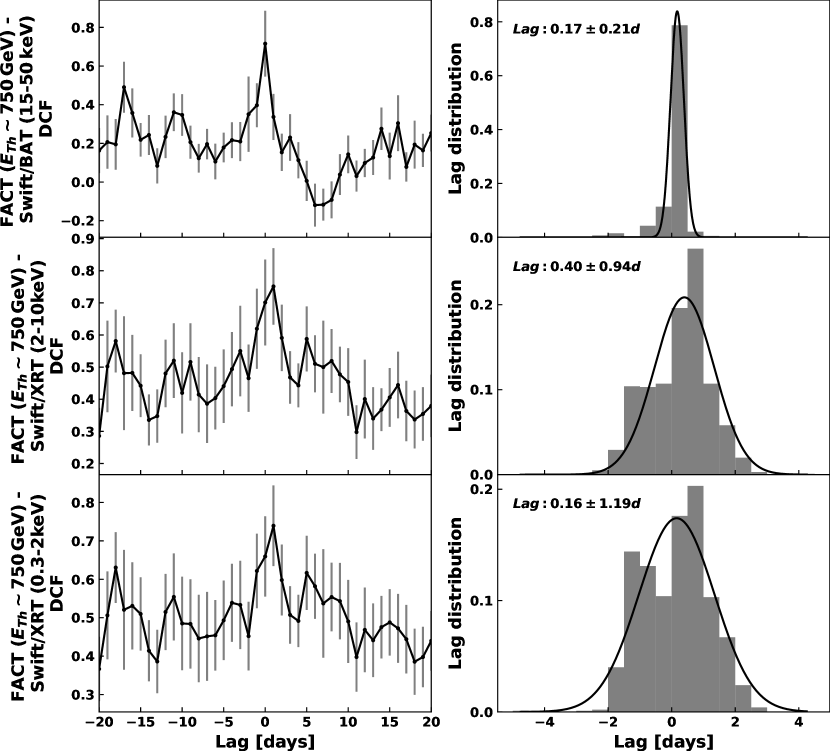
Figure 4: DCF cross-correlations of light curves (from top to bottom panel): FACT with Swift/BAT, Swift/XRT (2-10 keV), and Swift/XRT (0.3-2 keV). One-day binning was used. Left: DCF values as a function of lag. Grey error bars are 1$\sigma$ uncertainties. Right: Lag distributions derived from FR/RSS simulations (more details are provided in Sect. 3.3). A Gaussian fit (black lines) was used to derive the lag indicated in the plots.

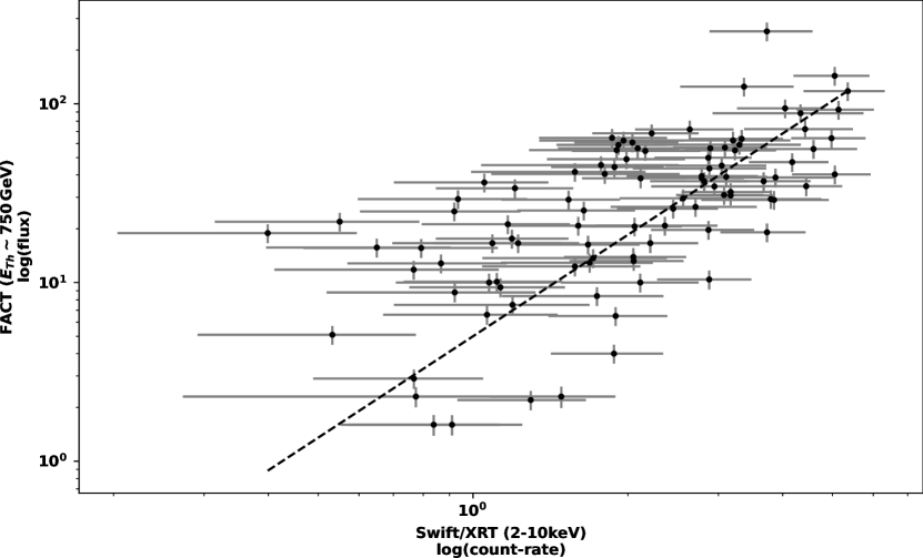
Figure 5: TeV (FACT) flux and X-ray (Swift/XRT 2-10 keV) count-rate measured within 24 hours (slope $1.89\pm 0.15$).

3.3 TeV / X-ray correlation

A strong correlation reaching 0.7 at 0 lag is found between the TeV (FACT) and X-ray (Swift/XRT or Swift/BAT) light curves (Fig. 4). The correlation peak is wider for Swift/XRT because of the larger (1-2 days) relative time distances between the FACT and Swift/XRT observations. In case of Swift/BAT, observations are coincident (within a day) with the FACT light curve.

The lag probability distributions reported in Fig. 4 are obtained from Monte Carlo simulations (as in Peterson et al., 1998). We generated $10^{4}$ subsets for each pair of light curves using flux randomisation (FR) and random subset selection (RSS) and calculated the resulting DCFs to obtain a representative time lag distributions using a centroid threshold of 80% of the DCF maximum (Peterson et al., 2004). The lag uncertainty corresponds to the standard deviation of the distribution of the lag values obtained for the random subsets.

The best estimate of the TeV/X-ray lag of $(0.17\pm 0.2)$ days is obtained by correlating the TeV and hard X-ray Swift/BAT light curves. Summing the time-lag distributions obtained from soft and hard X-rays increases the uncertainty to $(0.3\pm 0.4)$ days. This TeV/X-ray correlation in Mrk 501 was already reported using shorter and sparser data sets (Pandey et al., 2017; Ahnen et al., 2018).

As noted earlier, the TeV variability is stronger than in the X-rays, with a flux correlation slope (Fig. 5) increasing from $1.3\pm 0.1$ (with reference to the variability observed by Swift/XRT 0.3-2 keV) to $1.89\pm 0.15$ if Swift/XRT 2-10 keV is used. The dispersion of the data points in Fig. 5 around the main correlation, obtained using the orthogonal distance regression method, is compatible with intra-day variability in these bands or/and by spectral variations between flares. To build the correlation plots (Fig. 5 and Fig. 10), only coincident FACT and Swift/XRT observations were considered with measurements in time separation of less than 12 hours.

Bayesian Block algorithm was used to identify individual flares in the TeV and X-rays bands. The algorithm properly takes the significance of the data points into account, so that we applied it to the unfiltered data (see Sect. 2 and Fig. 1, where the uncleaned light curves are shown). The Bayesian Block algorithm was tuned for a false-positive probability of 1% (Scargle et al., 2013). A flare is defined as a significant change in flux (3$\sigma$) with a duration of at least one binning point. Thirty-seven TeV flares were identified. To enhance the detection of X-ray flares, we compiled a list of individual flares detected by Swift/BAT and Swift/XRT separately. Unfortunately, as the X-ray data were still often either too sparse or too noisy, we finally considered only 15 TeV flares (56330 – 56355, 56462 – 56465, 56467 – 56472, 56491 – 56498, 56536 – 56540, 56541 – 56545, 56815 – 56818, 56831 – 56833, 56856 – 56862, 56874 – 56883, 56887 – 56893, 56936 – 56944, 57156 – 57171, 57230 – 57235, and 57483 – 57489), with simultaneous coverage in X-rays. All of them coincide with individual X-ray flares or with periods with some level of X-ray flaring activity. TeV and X-ray flares have a similar duration. Most flares last less than seven days, confirming the cross-correlation results.

3.4 GeV / soft X-ray correlation

The GeV and soft X-ray variations appear strongly correlated on long timescales, as depicted in Fig. 6 (top panel). The GeV light curve is not correlated with the hard X-ray (Swift/BAT) or TeV light curves, however. This indicates that the GeV variability is not simultaneous to the flares lasting a few days, but is dominated by the long-lasting variations. This behaviour may be biased by the low sensitivity in the GeV band, and should only be considered along with other temporal data.

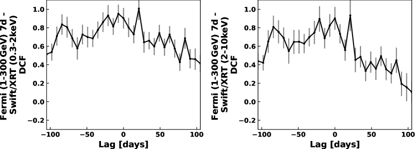
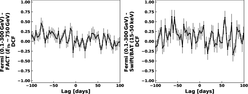
Figure 6: Cross-correlation of the GeV Fermi-LAT light curve with the data from Swift/XRT 0.3-2 keV (top right), Swift/XRT 2-10 keV (top left), FACT (bottom right), and Swift/BAT (bottom left). The time resolution is seven days. The grey error bars denote 1$\sigma$ uncertainties.

3.5 Correlations at/with longer wavelengths

We find a strong (reaching 0.85) but broad correlation between the optical and ultraviolet variations (Fig. 7), and both are broadly correlated with the radio light curve. Lags between the bands cannot be reliably estimated from the cross-correlations alone (Fig. 3).

The correlation between the GeV and radio light curves also appears strong (reaching 0.8), with radio lagging behind the GeV by 170-250 days. GeV-radio delays have also been reported in various sources by Max-Moerbeck et al. (2014), and were interpreted as shocks propagating in the jet.

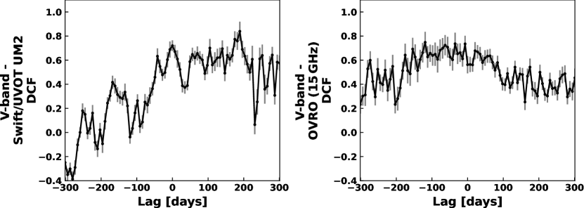
Figure 7: Multi-wavelength correlations for different bands. Left: Cross-correlation of the V-band and Swift/UVOT light curves. Right: Cross-correlation V-band and radio light curves. Grey error bars denote 1$\sigma$ uncertainties.

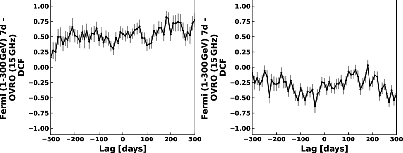
Figure 8: Multi-wavelength correlations for different bands. Left: Cross-correlation of the Fermi-LAT and radio light curves in the time range of [56800, 58226] MJD. Right: Cross-correlation of the Fermi-LAT and radio light curves in the time range of [54693, 56800] MJD using data from (Max-Moerbeck et al., 2014). Grey error bars denote 1$\sigma$ uncertainties.

The radio-GeV behaviour of Mrk 501 appears very different before the period considered in this study, however. Before MJD 56800, no correlation could be found (Fig. 8) using the data from Max-Moerbeck et al. (2014). All the other flux correlations derived above for the full data set do not change notably when data either before or after MJD 56800 are selected. The source may experience an internal change (misalignment due to the precession of a mini-jet, emission region properties change, etc.), which yields different behaviour and inter-band connection before and after 56800 MJD. It is important to note that this change is not related to the source flaring activity state, and there is no such change after 57600 MJD, for example, when Mrk 501 reaches a quiescent state in most bands (Fig. 1).

3.6 Spectral variations

The long-term duration of our campaign allows us to study the connection between spectral components. In the X-rays, we find a clear indication for a long-term harder-when-brighter behaviour (Fig. 9). The variability amplitude increases at harder X-rays right of the low-energy hump maximum in the SED (Fig.  9). Along with Fig. 5, this indicates a higher variability beyond the cut-off energies of both spectral components. The colour-colour diagram, showing the ratios of the TeV and GeV fluxes and of the hard and soft X-rays fluxes, respectively (Fig. 10), confirms the relation between the two spectral components and that the variability amplitude of the high-energy component is higher than that of the low-energy component.

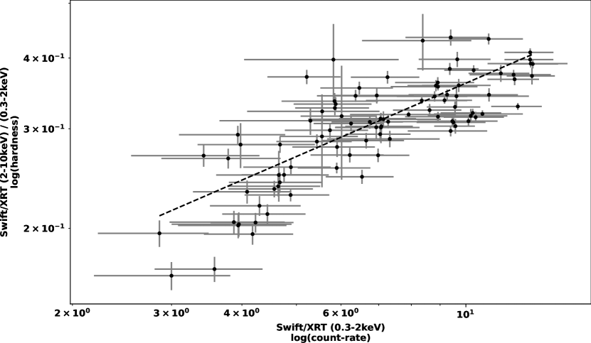
Figure 9: Ratio of Swift/XRT hard-to-soft vs Swift/XRT 0.3-2 keV count rate. The slope is $0.43\pm 0.04$.

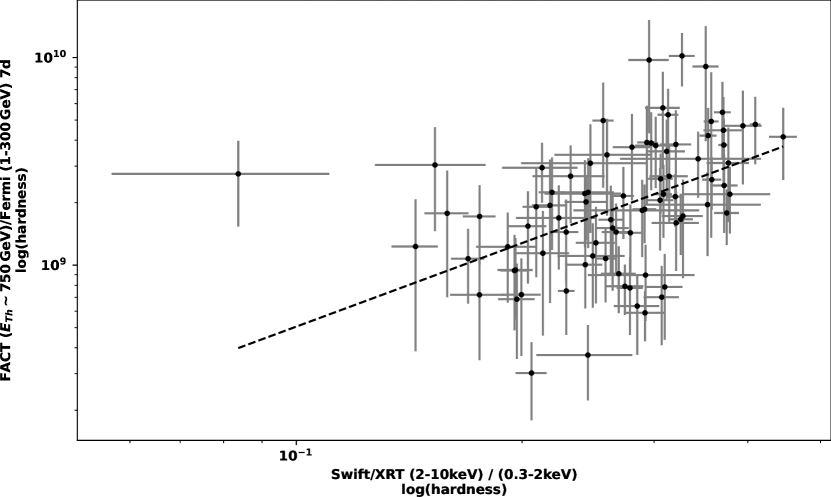
Figure 10: Ratio of TeV to GeV fluxes vs the ratio of Swift/XRT hard-to-soft flux. The slope is $1.4\pm 0.3$.

4 Discussion

4.1 Summary of results

We studied the broadband variability of Mrk 501 from the end of 2012 to the middle of 2018. Data from eight instruments were considered. During this period, the source experienced numerous flaring periods in the TeV. The highest flux was measured in 2014.

The variability was detected in all wave bands. The fractional variability is lowest in the radio ($F_{var}\sim 0.05$) and highest in the TeV ($F_{var}\sim 1.1$), and it monotonically increases from the radio to the X-rays and from the GeVs to the TeVs. A similar fractional variability pattern was reported for Mrk 421 on monthly (Aleksić et al., 2015b) and yearly (Ahnen et al., 2016) timescales. In the context of the one-zone synchrotron-self-Compton (SSC) model, this variability pattern indicates that the electron spectrum is more variable at higher energies. For the same period of observations, Mrk 501 is less variable than another nearby and bright HBL blazar Mrk 421 (Arbet-Engels et al., 2021).

To determine correlations between the spectral bands, we calculated the discrete-correlation functions for pairs of light curves and found that the X-ray and TeV emission is well correlated with a lag $<0.4$ days $(1\sigma)$. All the flares detected in the TeV band were coincident with X-ray flares.

The fractional variability and the correlated TeV and X-ray emission are likely produced by a synchronous change of the spectral shape of the low- (X-rays) and high-energy (TeV) components. A zero-lag correlation between the X-ray and TeV light curves suggests that the variations in the two bands are driven by a common physical process operating in the same emission region. We compare the observational constraints to different models in the next subsections, assuming that the flares are related to particles accelerated in shocks.

The radio and GeV emissions were correlated during the majority of the campaign (after about 56800 MJD), but not in older data (Fig. 8, left and right), indicating that the long-term radio emission showing the least variability originates from several components. The VLBA high-resolution radio images at 43 GHz indeed reveal an off-axis jet component (Koyama, S. et al., 2016) that may explain that the GeV and radio are not always correlated (see also Giroletti et al., 2008; Koyama et al., 2016). In July 2014, the radio-optical emission of Mrk 501 was also interpreted as a separate spectral component with little contribution in the GeV (MAGIC Collaboration et al., 2020).

4.2 Synchrotron self- or external Compton emission

In the quiescent state, several multi-wavelength campaigns of Mrk 501 reported that its spectral energy distribution was compatible with a one-zone SSC model with a Doppler beaming factor $\delta\approx 12-21$. (MAGIC Collaboration et al., 2020; Lei et al., 2018; Abdo et al., 2011a; Albert et al., 2007b). Additional spectral features detected during flares (MAGIC Collaboration et al., 2020; Lei et al., 2018; Ahnen et al., 2017) led to higher $\delta\approx 10-50$. The wide range of $\delta$ values can be explained by a deceleration of the jet (Georganopoulos & Kazanas, 2003) or by a radial structure with an inner fast spine and a slower outer layer where the radio emission is produced (Ghisellini et al., 2005). In both cases, the expected variability increases with frequency and should be lowest in the radio.

One of the most significant constraints on the size of the emitting region can be derived from the variability timescale. As expected from geometrical properties of a homogeneous source of incoherent, isotropic comoving-frame emission with a comoving size $R$, the minimum expected variability timescale can be written as $t_{var_{min}}=(1+z)R/(\delta c)$ (where $z$ is the source redshift). The shortest doubling timescale observed in Mrk 501 is 2 minutes (Abdo et al., 2011a), and the delay between various VHE bands is 4 minutes (an indication for progressive electron acceleration) indicate a gamma-ray source size $<10^{12}$ km.

Variability can also be constrained by the synchrotron cooling timescale. Synchrotron cooling time in the observer’s frame of reference can be written as $t_{cool,\,e}\approx 15.86\times 10^{11}\left((1+z)/\delta\right)^{1/2}\,(B/1{\rm G})^{-3/2}(\nu/1{\rm Hz})^{-1/2}\,{\rm seconds}$ (Zhang et al., 2019), where $\nu$ is the emission frequency. Using typical values of $B$ from $0.01$ to $0.31$ G, and $\delta$ from 12 to 25 (Abdo et al., 2011a; Ahnen et al., 2017), we can find that the synchrotron cooling times in the observer frame become shorter than 9 minutes, 2 hours, 7 hours, and 176 days for 50 keV, 0.3 keV, in the V-band, and in the radio, respectively. These timescales are much shorter than those shown in the auto-correlations. The duration of the flares should therefore be driven by physical changes of the emitting source(s) occurring on dynamical time scales.

The reported delay $<0.4$ days between the TeV and X-rays fluxes agrees with the self-Compton or external Compton frameworks as electrons cool rapidly $(<0.5\,{\rm hour})$ at these energies. The observed connection between the X-ray and TeV emission (Fig. 5) also supports the SSC model scenario of inverse Compton production of VHE gamma-rays by the same population of electrons. The relation between the X-ray and gamma-ray spectral breaks (Fig. 10) finally indicates that the cut-off energies of both spectral components are also related.

Assuming self-Compton emission for the TeV $\gamma$-rays (Mrk 501 is always in the Thomson regime in the TeV, e.g. Murase et al., 2012), the scenario with the stronger magnetic field produces a minute-variability timescale, which is close to the observations ( Abdo et al. (2011a)). Taking the compactness of the VHE source region into account, high Doppler factors ($\delta_{flaring}>40$, $\delta_{lowstate}>30$) (Cologna et al., 2017) are needed to avoid $\gamma$-ray absorption. An explanation for the fast TeV variability may also come from MHD turbulent flows or phase transitions (Krishan & Wiita, 1994), instabilities of hydrodynamic flows (Subramanian et al., 2012), or jet or mini-jet beaming turbulences on different scales (Crusius-Waetzel & Lesch, 1998; Giannios et al., 2010).

In the one-zone synchrotron regime, the energy cutoff and the flux normalisation are controlled by $B$, $\delta,$ and the particle spectrum. Variations in these parameters can lead to independent GeV and TeV variability (as indicated by the observations, see Fig. 6). In addition, in the shock-in-jet model, the regions emitting X-rays and TeVs are closer to the black hole than those responsible for the bulk of the optical-radio and the GeV emissions. In the SSC frame, the observed correlations between TeV and X-rays (fluxes and spectral slopes), radio, and GeV fluxes, and the lack of correlations between the TeVs/X-rays and GeVs would require that some of the above physical parameter(s) is/are changing along the jet.

4.3 Hadronic and lepto-hadronic radiation scenarios

In addition to pure leptonic scenarios, in which all radiation is produced by relativistic electrons, purely hadronic models (Mücke & Protheroe, 2001a) and lepto-hardronic models were also proposed (Mastichiadis et al., 2013; Petropoulou et al., 2016; Mücke & Protheroe, 2001b, a; Galanti et al., 2020; Mannheim, 1993).

In lepto-hadronic models, the low-energy SED component is still dominated by the synchrotron emission of primary accelerated electrons. However, the high-energy SED component is dominated by proton synchrotron and/or pion-decay-induced pair cascades. The correlation between the TeV and the X-ray flares indicates that electrons and protons are accelerated in the same region. As the proton acceleration time $t_{acc}=20\,\xi\,\gamma\,m_{p}c/3\,eB\geq 10\,\xi\ {\rm days}$ (where $\xi\geq 1$ is the mean free path in units of Larmor radius, Kusunose et al., 2000; Inoue & Takahara, 1996) is much longer than the delay observed between the TeV and X-ray light curves, the driving mechanism of the variability should be linked to some dynamical processes (e.g. changing orientation or beaming of the relativistically moving emission region) in combination with propagation effects. However, the absence of a correlation between the GeV and TeV bands on the same timescale as observed for the TeV/X-ray correlation suggests that the variability of the hadronic component is not driven by the process behind the variability of the leptonic component.

Hadronic emission models propose proton synchrotron to be responsible for the low-energy SED component and pion-induced cascades for the high-energy component (Mastichiadis et al.2013). These models require strong magnetic fields (¿10 G) such that the Larmor radius of the protons remains smaller than the jet radius (Sikora, 2011). In these conditions and assuming that the X-ray emission is from proton synchrotron, the expected cooling timescale of tens of hours (Zhang et al., 2019) is also inconsistent with observations. Variability on shorter timescales may again possibly be driven by dynamical processes, which affect the whole population of relativistic particles, but as above, this is not consistent with the absence of a GeV/TeV correlation and with radio lagging behind the GeV by about 200 days.

The mechanisms responsible for the broadband emission of blazar jets, accelerating electrons should in principle also accelerate protons and heavier nuclei possibly related to the observed ultra high-energy cosmic rays (UHECRs). When these particles interact with the surrounding photons, $\gamma$-rays and neutrinos may be produced (Padovani et al., 2018; Ansoldi et al., 2018; Mannheim, 1993). Muons and pions created in these processes will also be affected by the proton acceleration time, so that timescales observed in the TeV cannot be reproduced with this mechanism (Zech et al., 2017). In addition, Pion photoproduction is generally inefficient because protons mostly lose energy through synchrotron radiation (but see Rachen & Mészáros, 1998).

4.4 Flare timing

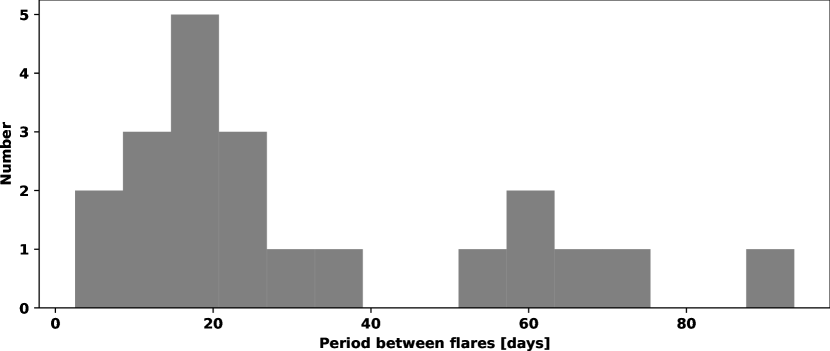
Figure 11: Period between peaks of 37 identified TeV flares, 15 of which have good X-ray coverage and are listed in Sect. 3.3.

The mass of the supermassive black hole (SMBH) of Mrk 501 is estimated as $0.9-3.4\times 10^{9}M_{\odot}$ (Barth et al., 2002). The distribution of the time delays between maximums of identified TeV flares peaks between 5 and 25 days (Fig. 11) (undetected flares could mimic longer delays). These delays correspond to $\sim 10^{4}\ R_{G}/c\sim 17$ days, which could be expected if the flares were related to Lense-Thirring (Thirring, 1918) precession of a misaligned accretion disk (Bardeen & Petterson, 1975; Liska et al., 2017). The inter-flare period originating from such a precession is shortened in the source rest frame by a factor $\Gamma$, then, for the observer, it becomes shortened by a factor $\Gamma^{-1}$, which compensate for each other.

5 Conclusions

The analysis of about 5.5 years of light curves from eight instruments yields the following main observational results:

1. The strongest variations were found in TeV and X-rays. The TeV and X-ray fluxes measured simultaneously (within 24 hours) are correlated, as are the X-ray and gamma-ray spectral breaks, as expected from SSC models. The lag between the TeV and X-ray variations could be estimated as $<0.4$ days $(1\sigma)$.

2. The characteristic time interval between TeV flares is comparable with the expectation if these flares are triggered by a Lense-Thirring precession of the accretion disk around the SMBH.

The observed variability of Mrk 501 was compared with the predictions of leptonic, lepto-hadronic, and hadronic models. We found that purely hadronic models are incompatible with the observations due to extremely long synchrotron cooling time in the radio and relatively short GeV-radio delay. The lepto-hadronic models are also incompatible with observations because they fail to reproduce simultaneously the short lag observed between X-rays and TeV and the absence of correlation between the GeV and TeV. Electron synchrotron self- or external Compton processes match the observations of Mrk 501 in general, although individual flares may require more complex models, including the introduction of a second emission zone (Abdo et al., 2011b; Sahu et al., 2020a; Ahnen et al., 2018).

References

- Abdo et al. (2011a) Abdo, A. A., Ackermann, M., Ajello, M., et al. 2011a, ApJ, 727, 129
- Abdo et al. (2011b) Abdo, A. A., Ackermann, M., Ajello, M., et al. 2011b, ApJ, 727, 129
- Abdo et al. (2009) Abdo, A. A., Ackermann, M., Ajello, M., et al. 2009, Astroparticle Physics, 32, 193
- Abdo et al. (2011c) Abdo, A. A., Ackermann, M., Ajello, M., et al. 2011c, ApJ, 736, 131
- Abdollahi et al. (2020) Abdollahi, S., Acero, F., Ackermann, M., et al. 2020, ApJS, 247, 33
- Abeysekara et al. (2017) Abeysekara, A. U., Albert, A., Alfaro, R., et al. 2017, ApJ, 841, 100
- Acciari et al. (2011a) Acciari, V. A., Aliu, E., Arlen, T., et al. 2011a, ApJ, 738, 25
- Acciari et al. (2011b) Acciari, V. A., Arlen, T., Aune, T., et al. 2011b, ApJ, 729, 2
- Ackermann et al. (2012a) Ackermann, M., Ajello, M., Albert, A., et al. 2012a, ApJS, 203, 4
- Ackermann et al. (2012b) Ackermann, M., Ajello, M., Allafort, A., et al. 2012b, Astroparticle Physics, 35, 346
- Aharonian et al. (2001) Aharonian, F., Akhperjanian, A., Barrio, J., et al. 2001, ApJ, 546, 898
- Aharonian et al. (1999) Aharonian, F. A., Akhperjanian, A. G., Barrio, J. A., et al. 1999, A&A, 349, 11
- Ahnen et al. (2016) Ahnen, M. L., Ansoldi, S., Antonelli, L. A., et al. 2016, A&A, 593, A91
- Ahnen et al. (2017) Ahnen, M. L., Ansoldi, S., Antonelli, L. A., et al. 2017, A&A, 603, A31
- Ahnen et al. (2018) Ahnen, M. L., Ansoldi, S., Antonelli, L. A., et al. 2018, A&A, 620, A181
- Albert et al. (2007a) Albert, J., Aliu, E., Anderhub, H., et al. 2007a, ApJ, 663, 125
- Albert et al. (2007b) Albert, J., Aliu, E., Anderhub, H., et al. 2007b, ApJ, 669, 862
- Aleksić et al. (2015a) Aleksić, J., Ansoldi, S., Antonelli, L. A., et al. 2015a, A&A, 573, A50
- Aleksić et al. (2015b) Aleksić, J., Ansoldi, S., Antonelli, L. A., et al. 2015b, A&A, 576, A126
- Aleksić et al. (2015c) Aleksić, J., Ansoldi, S., Antonelli, L. A., et al. 2015c, A&A, 578, A22
- Aliu et al. (2016) Aliu, E., Archambault, S., Archer, A., et al. 2016, A&A, 594, A76
- Anderhub et al. (2013) Anderhub, H., Backes, M., Biland, A., et al. 2013, Journal of Instrumentation, 8, P06008
- Ansoldi et al. (2018) Ansoldi, S., Antonelli, L. A., Arcaro, C., et al. 2018, ApJ, 863, L10
- Arbet-Engels et al. (2021) Arbet-Engels, A., Baack, D., Balbo, M., et al. 2021, A&A, 647, A88
- Atwood et al. (2009) Atwood, W. B., Abdo, A. A., Ackermann, M., et al. 2009, ApJ, 697, 1071
- Bardeen & Petterson (1975) Bardeen, J. M. & Petterson, J. A. 1975, ApJ, 195, L65
- Barth et al. (2002) Barth, A. J., Ho, L. C., & Sargent, W. L. W. 2002, The Astrophysical Journal, 566, L13
- Bartoli et al. (2012) Bartoli, B., Bernardini, P., Bi, X. J., et al. 2012, ApJ, 758, 2
- Baumgartner et al. (2013) Baumgartner, W. H., Tueller, J., Markwardt, C. B., et al. 2013, ApJS, 207, 19
- Beck et al. (2019) Beck, M., Arbet-Engels, A., Baack, D., et al. 2019, 36, 630
- Biland et al. (2014) Biland, A., Bretz, T., Buß, J., et al. 2014, Journal of Instrumentation, 9, P10012
- Bretz (2019) Bretz, T. 2019, Astroparticle Physics, 111, 72
- Bretz et al. (2013) Bretz, T., Biland, A., Buß, J., et al. 2013, arXiv e-prints [arXiv:1308.1516]
- Bretz & Dorner (2010) Bretz, T. & Dorner, D. 2010, in Astroparticle, Particle and Space Physics, Detectors and Medical Physics Applications, ed. C. Leroy, P.-G. Rancoita, M. Barone, A. Gaddi, L. Price, & R. Ruchti, 681–687
- Burrows et al. (2005) Burrows, D. N., Hill, J. E., Nousek, J. A., et al. 2005, Space Sci. Rev., 120, 165
- Cologna et al. (2017) Cologna, G., Chakraborty, N., Jacholkowska, A., et al. 2017, in American Institute of Physics Conference Series, Vol. 1792, 6th International Symposium on High Energy Gamma-Ray Astronomy, 050019
- Crusius-Waetzel & Lesch (1998) Crusius-Waetzel, A. R. & Lesch, H. 1998, A&A, 338, 399
- Dorner et al. (2017) Dorner, D., Adam, J., Ahnen, L. M., et al. 2017, International Cosmic Ray Conference, 35, 609
- Dorner et al. (2015) Dorner, D., Ahnen, M. L., Bergmann, M., et al. 2015, ArXiv e-prints [arXiv:1502.02582]
- Edelson & Krolik (1988) Edelson, R. A. & Krolik, J. H. 1988, ApJ, 333, 646
- Evans et al. (2009) Evans, P. A., Beardmore, A. P., Page, K. L., et al. 2009, MNRAS, 397, 1177
- Fomin et al. (1994) Fomin, V. P., Stepanian, A. A., Lamb, R. C., et al. 1994, Astroparticle Physics, 2, 137
- Galanti et al. (2020) Galanti, G., Tavecchio, F., & Landoni, M. 2020, MNRAS, 491, 5268
- Gehrels & Swift Team (2004) Gehrels, N. & Swift Team. 2004, New Astronomy Reviews, 48, 431
- Georganopoulos & Kazanas (2003) Georganopoulos, M. & Kazanas, D. 2003, New A Rev., 47, 653
- Ghisellini et al. (2005) Ghisellini, G., Tavecchio, F., & Chiaberge, M. 2005, A&A, 432, 401
- Giannios et al. (2010) Giannios, D., Uzdensky, D. A., & Begelman, M. C. 2010, MNRAS, 402, 1649
- Giroletti et al. (2008) Giroletti, M., Giovannini, G., Cotton, W. D., et al. 2008, A&A, 488, 905
- Hildebrand et al. (2017) Hildebrand, D., Ahnen, M. L., Balbo, M., et al. 2017, International Cosmic Ray Conference, 35, 779
- Inoue & Takahara (1996) Inoue, S. & Takahara, F. 1996, ApJ, 463, 555
- Knoetig et al. (2013) Knoetig, M. L., Biland, A., Bretz, T., et al. 2013, in International Cosmic Ray Conference, Vol. 33, International Cosmic Ray Conference, 1132
- Koyama et al. (2016) Koyama, S., Kino, M., Giroletti, M., et al. 2016, A&A, 586, A113
- Koyama, S. et al. (2016) Koyama, S., Kino, M., Giroletti, M., et al. 2016, A&A, 586, A113
- Krimm et al. (2013) Krimm, H. A., Holland, S. T., Corbet, R. H. D., et al. 2013, The Astrophysical Journal Supplement Series, 209, 14
- Krishan & Wiita (1994) Krishan, V. & Wiita, P. J. 1994, ApJ, 423, 172
- Kusunose et al. (2000) Kusunose, M., Takahara, F., & Li, H. 2000, ApJ, 536, 299
- Lei et al. (2018) Lei, M., Yang, C., Wang, J., & Yang, X. 2018, PASJ, 70, 45
- Liska et al. (2017) Liska, M., Hesp, C., Tchekhovskoy, A., et al. 2017, Monthly Notices of the Royal Astronomical Society: Letters, 474, L81
- MAGIC Collaboration et al. (2020) MAGIC Collaboration, Acciari, V. A., Ansoldi, S., et al. 2020, A&A, 637, A86
- Mahlke et al. (2017) Mahlke, M., Bretz, T., Adam, J., et al. 2017, International Cosmic Ray Conference, 35, 612
- Mannheim (1993) Mannheim, K. 1993, A&A, 269, 67
- Mastichiadis et al. (2013) Mastichiadis, A., Petropoulou, M., & Dimitrakoudis, S. 2013, MNRAS, 434, 2684
- Max-Moerbeck et al. (2014) Max-Moerbeck, W., Hovatta, T., Richards, J. L., et al. 2014, MNRAS, 445, 428
- Mücke & Protheroe (2001a) Mücke, A. & Protheroe, R. J. 2001a, Astroparticle Physics, 15, 121
- Mücke & Protheroe (2001b) Mücke, A. & Protheroe, R. J. 2001b, International Cosmic Ray Conference, 3, 1153
- Murase et al. (2012) Murase, K., Dermer, C. D., Takami, H., & Migliori, G. 2012, ApJ, 749, 63
- Padovani et al. (2018) Padovani, P., Giommi, P., Resconi, E., et al. 2018, MNRAS, 480, 192
- Pandey et al. (2017) Pandey, A., Gupta, A. C., & Wiita, P. J. 2017, ApJ, 841, 123
- Peterson et al. (2004) Peterson, B. M., Ferrarese, L., Gilbert, K. M., et al. 2004, ApJ, 613, 682
- Peterson et al. (1998) Peterson, B. M., Wanders, I., Horne, K., et al. 1998, PASP, 110, 660
- Petropoulou et al. (2016) Petropoulou, M., Coenders, S., & Dimitrakoudis, S. 2016, Astroparticle Physics, 80, 115
- Piner et al. (2010) Piner, B. G., Pant, N., & Edwards, P. G. 2010, ApJ, 723, 1150
- Poutanen et al. (2008) Poutanen, J., Zdziarski, A. A., & Ibragimov, A. 2008, MNRAS, 389, 1427
- Quinn et al. (1996) Quinn, J., Akerlof, C. W., Biller, S., et al. 1996, ApJ, 456, L83
- Rachen & Mészáros (1998) Rachen, J. P. & Mészáros, P. 1998, Phys. Rev. D, 58, 123005
- Richards et al. (2011) Richards, J. L., Max-Moerbeck, W., Pavlidou, V., et al. 2011, ApJS, 194, 29
- Roming et al. (2005) Roming, P. W. A., Kennedy, T. E., Mason, K. O., et al. 2005, Space Sci. Rev., 120, 95
- Roming et al. (2009) Roming, P. W. A., Koch, T. S., Oates, S. R., et al. 2009, ApJ, 690, 163
- Sahu et al. (2020a) Sahu, S., López Fortín, C. E., Castañeda Hernández, L. H., Nagataki, S., & Rajpoot, S. 2020a, ApJ, 901, 132
- Sahu et al. (2020b) Sahu, S., López Fortín, C. E., Iglesias Martínez, M. E., Nagataki, S., & Fernández de Córdoba, P. 2020b, MNRAS, 492, 2261
- Scargle et al. (2013) Scargle, J. D., Norris, J. P., Jackson, B., & Chiang, J. 2013, ApJ, 764, 167
- Schlafly & Finkbeiner (2011) Schlafly, E. F. & Finkbeiner, D. P. 2011, ApJ, 737, 103
- Schleicher et al. (2019) Schleicher, B., Arbet-Engels, A., Baack, D., et al. 2019, Galaxies, 7, 62
- Shukla et al. (2015) Shukla, A., Chitnis, V. R., Singh, B. B., et al. 2015, ApJ, 798, 2
- Sikora (2011) Sikora, M. 2011, in Jets at All Scales, ed. G. E. Romero, R. A. Sunyaev, & T. Belloni, Vol. 275, 59–67
- Simonetti et al. (1985) Simonetti, J. H., Cordes, J. M., & Heeschen, D. S. 1985, ApJ, 296, 46
- Smith et al. (2009) Smith, P. S., Montiel, E., Rightley, S., et al. 2009, arXiv e-prints [arXiv:0912.3621]
- Subramanian et al. (2012) Subramanian, P., Shukla, A., & Becker, P. A. 2012, MNRAS, 423, 1707
- Tanihata et al. (2001) Tanihata, C., Urry, C. M., Takahashi, T., et al. 2001, ApJ, 563, 569
- Temme et al. (2015) Temme, F., Ahnen, M. L., Balbo, M., et al. 2015, in International Cosmic Ray Conference, Vol. 34, 34th International Cosmic Ray Conference (ICRC2015), 707
- Thirring (1918) Thirring, H. 1918, Physikalische Zeitschrift, 19, 33
- Tueller et al. (2010) Tueller, J., Baumgartner, W. H., Markwardt, C. B., et al. 2010, ApJS, 186, 378
- Vaughan et al. (2003) Vaughan, S., Edelson, R., Warwick, R. S., & Uttley, P. 2003, MNRAS, 345, 1271
- Zech et al. (2017) Zech, A., Cerruti, M., & Mazin, D. 2017, A&A, 602, A25
- Zhang et al. (2019) Zhang, Z., Gupta, A. C., Gaur, H., et al. 2019, ApJ, 884, 125