Adaptive variational Bayes: Optimality, computation and applications

Abstract

In this paper, we explore adaptive inference based on variational Bayes. Although several studies have been conducted to analyze the contraction properties of variational posteriors, there is still a lack of a general and computationally tractable variational Bayes method that performs adaptive inference. To fill this gap, we propose a novel adaptive variational Bayes framework, which can operate on a collection of models. The proposed framework first computes a variational posterior over each individual model separately and then combines them with certain weights to produce a variational posterior over the entire model. It turns out that this combined variational posterior is the closest member to the posterior over the entire model in a predefined family of approximating distributions. We show that the adaptive variational Bayes attains optimal contraction rates adaptively under very general conditions. We also provide a methodology to maintain the tractability and adaptive optimality of the adaptive variational Bayes even in the presence of an enormous number of individual models, such as sparse models. We apply the general results to several examples, including deep learning and sparse factor models, and derive new and adaptive inference results. In addition, we characterize an implicit regularization effect of variational Bayes and show that the adaptive variational posterior can utilize this.

SReferences

and

1 Introduction

The bias-variance trade-off, a fundamental principle of statistical inference, suggests that a statistical model needs to be appropriately chosen in order to gain useful information from data efficiently. For example, in nonparametric regression or density estimation, the complexity of a model should be selected or specified according to the smoothness of the true regression function or density to optimize the prediction or estimation risk. Another example is high-dimensional linear regression, where it is almost necessary to impose certain sparsity on the regression coefficients to reduce statistical variability in high-dimensional estimation. It will be easier to determine a suitable model when we have some knowledge of the underlying data-generating process. However, this knowledge is rarely available in practice. Therefore, accurate inference requires the statistical method to be adaptive, i.e., to be able to learn from data the relevant features of the data-generating process so that appropriate model determinations can be made.

From this adaptive inference viewpoint, Bayesian inference is appealing. Given a collection of models, a Bayesian procedure can automatically learn the appropriate model via a hierarchical prior design, which first assigns a prior over models followed by a prior on the parameter given the selected model. A number of studies (Belitser and Ghosal, 2003; Lember and van der Vaart, 2007; Ghosal et al., 2008; Arbel et al., 2013; Gao et al., 2020; Han, 2021) have shown that with a carefully designed hierarchical prior, one can conduct optimal inference adaptively using the (original) posterior distribution. However, posterior inference based on sampling the posterior distribution over different models is usually computationally demanding and often very inefficient, especially when moves between models are poorly proposed in a Markov chain Monte Carlo (MCMC) algorithm.

High-dimensional and/or huge data sets have been more frequent in practical applications, with which computing posterior distributions exactly by MCMC algorithms is time-consuming and even intractable. An attractive and popular alternative is variational Bayes that offers computationally fast approximations, called variational posteriors, of posterior distributions using optimization algorithms. Along with the increasing popularity of variational Bayes, theoretical analysis of variational posteriors has been conducted recently. Zhang and Gao (2020) provided mild and general sufficient conditions for establishing contraction rates of variational posteriors. Pati et al. (2018) and Yang et al. (2020) developed variational Bayes theoretic frameworks that can deal with latent variable models. Alquier and Ridgway (2020) investigated the contraction properties of variational fractional posteriors where the likelihood is replaced by its fractional version with a positive exponent less than 1. There are several studies that derived contraction rates of variational posteriors for a specific statistical model, for example, mixture models (Chérief-Abdellatif and Alquier, 2018), sparse (Gaussian) linear regression (Ray and Szabó, 2022; Yang and Martin, 2020), sparse logistic linear regression (Ray et al., 2020) and sparse factor models (Ning, 2021).

Nonetheless, the adaptivity of variational posteriors remains an important and largely open problem. Although the existing theoretical frameworks have produced adaptive variational Bayes methods for some specific models, they require specially designed prior distributions and variational families to achieve adaptivity, which restricts the theory’s usefulness. Another problem concerns computation. Construction of a computationally tractable variational Bayes method over a collection of models is not an easy task in general. Exceptionally, Zhang and Gao (2020) proposed a potentially adaptive variational Bayes procedure with an additional model selection stage, which we call model selection variational Bayes. They showed that after selecting the best model among multiple models and conducting variational inference over the selected model, the variational posterior arising from this process could be optimal under mild assumptions. Although not clearly stated, this procedure appears capable of achieving adaptive optimality in many problems. In Chérief-Abdellatif (2019), a similar model selection approach was applied to variational fractional posteriors and its theoretical properties were studied.

In this paper, we propose a new variational Bayes method, called adaptive variational Bayes. Instead of selecting the best model and using the variational posterior over the selected model for subsequent inference tasks, the proposed framework aggregates multiple variational posteriors, each of which is obtained for each individual model separately, with certain weights to produce a variational posterior over the entire model, referred to as the adaptive variational posterior. This aggregated variational posterior turns out to be a closer approximation to the original posterior than the variational posterior over the selected model. Theoretically, the adaptive variational posterior can attain optimal contraction rates adaptively for a wide variety of statistical problems under mild conditions on priors and variational families. To the best of our knowledge, our framework is the first general recipe for establishing the adaptive contraction of variational posteriors.

We summarized our contributions as follows.

1. Computational tractability. As we have mentioned previously, Bayesian inference via a posterior distribution over multiple models has been shown to be an adaptively optimal procedure in a wide range of statistical applications. Therefore naturally, it is desirable to approximate the posterior distribution over the entire model, which is not easy to compute and often intractable. We demonstrate that the adaptive variational posterior, which is an aggregate of individual variational posteriors, is the closest member to the posterior in a predefined family of approximating distributions. This implies that the adaptive variational Bayes can inherit the computational tractability of variational Bayes methods used for obtaining the individual variational posteriors as long as the model complexity is not too large.

2. Adaptive contraction rate and model selection consistency. We formulate mild conditions under which the adaptive variational posterior can attain optimal contraction rates adaptively. Our theoretical conditions are slightly simpler than those of Zhang and Gao (2020) in the sense that the “prior mass condition” can be “hidden”, and that a condition associated with a stronger divergence than the Kullback-Leibler divergence can be relaxed. We want to clarify that these technical simplifications are not related to any aspect of the proposed method, but are made by rearranging the proof of Zhang and Gao (2020). We also provide some easily verifiable sufficient conditions for our theoretical assumptions. Moreover, we show that the adaptive variational Bayes method does not severely overestimate and underestimate the “best” model that leads to an optimal contraction rate. We apply our general theory to deep neural network models and derive adaptive optimal contraction rates in a number of applications.

3. Extension to combinatorial model spaces. Although completely parallelizable, the computation of the adaptive variational posterior becomes intractable when the number of models is extremely large because of the need to obtain a variational posterior for every individual model. This is the case for statistical models involving a “combinatorial” model structure such as high-dimensional sparse linear regression, where the individual models may be divided by a sparse pattern of the regression coefficients. This is clearly different from a “nested” model space such as a mixture model, in which the individual models can be ordered by their complexity, such as the number of mixture components. We show that, however, the proposed approach can be applied to combinatorial model spaces by utilizing tailored priors and variational families. Our method is particularly useful for model spaces with both combinatorial and nested structures, such as sparse factor models and high-dimensional nonparametric regression, and we study these examples.

4. Regularization via variational approximation. In fact, under the theoretical conditions we formulate in our main theory, of which a key part is related to the choice of a prior, the original posterior distribution can contract adaptively also. In this regard, our theory does not reveal a theoretical merit of the adaptive variational posterior over the original posterior. However, we find that there is a situation where the adaptive variational posterior is guaranteed to behave well while the original posterior is not. This phenomenon, which we refer to as implicit variational Bayes regularization, comes from the choice of variational families.

5. Theoretical justification of the use of quasi-likelihood. We consider the use of quasi-likelihoods in the proposed adaptive variational Bayes framework. We formulate conditions on quasi-likelihoods under which adaptive contraction rates are achieved by variational quasi-posteriors. We apply the general result to stochastic block models and nonparametric regression with sub-Gaussian errors.

The rest of the paper is organized as follows. We first introduce some notation in the rest of this section. In Section 2, we develop a general framework for adaptive variational Bayes inference. Concretely, we provide a design of the prior distribution and variational family, and describe a general and simple scheme for computation of the proposed variational posterior. In Section 3, we study the contraction properties of the proposed variational posterior, including oracle rates, adaptivity and model selection properties. In Section 4, we apply our general results to variational deep learning. In Section 5, we propose an approach by which the adaptive variational Bayes is applicable even when the number of individual models is quite large. In Section 6, we study the implicit variational Bayes regularization and derive adaptive contraction rates using this regularization effect. In Section 7, we study the theoretical properties of variational quasi-posteriors where the usual likelihood function is replaced with an alternative quasi-likelihood.

1.1 Notation

Let $\mathbb{R}$, $\mathbb{R}_{+}$, $\mathbb{R}_{\geq 0}$, $\mathbbm{Z}$, $\mathbbm{N}_{0}$ and $\mathbbm{N}$ be the sets of real numbers, positive numbers, nonnegative numbers, integers, nonnegative integers and natural numbers, respectively. We denote by $\mathbbm{1}(\cdot)$ the indicator function. For two integers $z_{1},z_{2}\in\mathbbm{Z}$ with $z_{1}\leq z_{2}$, we let $[z_{1}\mathrel{\mathop{\mathchar 58\relax}}z_{2}]\mathrel{\mathop{\mathchar 58\relax}}=\mathinner{\left\{z\in\mathbbm{Z}\mathrel{\mathop{\mathchar 58\relax}}z_{1}\leq z\leq z_{2}\right\}}$ and if $z_{2}\geq 2$, we use the shorthand $[z_{2}]\mathrel{\mathop{\mathchar 58\relax}}=[1\mathrel{\mathop{\mathchar 58\relax}}z_{2}]$ and $\mathbbm{N}_{\geq z_{2}}\mathrel{\mathop{\mathchar 58\relax}}=\mathbbm{N}\setminus[z_{2}-1]=\mathinner{\left\{z\in\mathbbm{N}\mathrel{\mathop{\mathchar 58\relax}}z\geq z_{2}\right\}}$. For $d\in\mathbbm{N}$, let $\mathbf{0}_{d}$ and $\mathbf{1}_{d}$ denote the $d$-dimensional vectors of 0’s and of 1’s, respectively and let $\mathbf{I}_{d}$ denote the $d\times d$-dimensional identity matrix. For a $d$-dimensional vector $\mathbf{x}\mathrel{\mathop{\mathchar 58\relax}}=(x_{j})_{j\in[d]}\in\mathbb{R}^{d}$, we denote $|\mathbf{x}|_{q}\mathrel{\mathop{\mathchar 58\relax}}=\mathinner{(\sum_{j=1}^{d}|x_{j}|^{q})}^{1/q}$ for $q\geq 1$, which are the usual Euclidean $q$-norm, and denote $|\mathbf{x}|_{0}\mathrel{\mathop{\mathchar 58\relax}}=\sum_{j=1}^{d}\mathbbm{1}(x_{j}\neq 0)$ and $|\mathbf{x}|_{\infty}\mathrel{\mathop{\mathchar 58\relax}}=\max_{j\in[d]}|x_{j}|$. Let $\Delta_{d}\mathrel{\mathop{\mathchar 58\relax}}=\mathinner{\{\bm{\alpha}\in[0,1]^{d}\mathrel{\mathop{\mathchar 58\relax}}|\bm{\alpha}|_{1}=1\}}$. We denote by $\mathbbm{S}_{++}^{d}$ the set of $d\times d$ symmetric positive definite matrices. For a real number $x\in\mathbb{R}$, we define $\left\lfloor{x}\right\rfloor\mathrel{\mathop{\mathchar 58\relax}}=\max\{z\in\mathbbm{Z}\mathrel{\mathop{\mathchar 58\relax}}z\leq x\}$, and $\left\lceil{x}\right\rceil\mathrel{\mathop{\mathchar 58\relax}}=\min\{z\in\mathbbm{Z}\mathrel{\mathop{\mathchar 58\relax}}z\geq x\}$. For two real numbers $a,b\in\mathbb{R}$, we write $a\vee b\mathrel{\mathop{\mathchar 58\relax}}=\max\{a,b\}$ and $a\wedge b\mathrel{\mathop{\mathchar 58\relax}}=\min\{a,b\}$. Moreover, for two real vectors $\mathbf{a}\mathrel{\mathop{\mathchar 58\relax}}=(a_{j})_{j\in[d]}\in\mathbb{R}^{d}$ and $\mathbf{b}\mathrel{\mathop{\mathchar 58\relax}}=(b_{j})_{j\in[d]}\in\mathbb{R}^{d}$ with the same dimension, we write $\mathbf{a}\vee\mathbf{b}\mathrel{\mathop{\mathchar 58\relax}}=(a_{j}\vee b_{j})_{j\in[d]}$ and $\mathbf{a}\wedge\mathbf{b}\mathrel{\mathop{\mathchar 58\relax}}=(a_{j}\wedge b_{j})_{j\in[d]}$. For an arbitrary set $B$, we denote by $B^{\complement}$ its complement and by $|B|$ its cardinality. Let $\mathbbm{P}(B)$ be the powerset of $B$, i.e., $\mathbbm{P}(B)\mathrel{\mathop{\mathchar 58\relax}}=\{B^{\prime}\mathrel{\mathop{\mathchar 58\relax}}B^{\prime}\subset B\}$. For two positive sequences $(a_{n})_{n\in\mathbb{N}}$ and $(b_{n})_{n\in\mathbb{N}}$, we write $a_{n}\lesssim b_{n}$ or $b_{n}\gtrsim a_{n}$ or $a_{n}=\mathscr{O}(b_{n})$, if there exists a positive constant $C>0$ such that $a_{n}\leq Cb_{n}$ for any $n\in\mathbb{N}$. Moreover, we write $a_{n}\asymp b_{n}$ if both $a_{n}\lesssim b_{n}$ and $a_{n}\gtrsim b_{n}$ hold. We write $a_{n}=\mathscr{o}(b_{n})$ if $\lim_{n\to\infty}a_{n}/b_{n}=0.$ Absolute constants denoted by e.g., $\mathfrak{c}_{1},\mathfrak{c}_{2},\dots$ may vary from place to place.

For a measurable space $(\mathbbm{X},\mathcal{X})$, we denote by $\mathcal{P}(\mathbbm{X})$ the set of all probability measures supported on $\mathbbm{X}$. For a probability measure $\textsf{{P}}\in\mathcal{P}(\mathbbm{X})$ and a function $g$ on $\mathbbm{X}$, we write $\textsf{{P}}g\mathrel{\mathop{\mathchar 58\relax}}=\int_{\mathbbm{X}}g\textup{d}\textsf{{P}}$, i,e., $\textsf{{P}}g$ denotes the expectation of $g$ with respect to the measure P. For two probability distributions $\textsf{{P}}_{1}\in\mathcal{P}(\mathbbm{X})$ and $\textsf{{P}}_{2}\in\mathcal{P}(\mathbbm{X})$, we denote by $\textup{KL}(\textsf{{P}}_{1},\textsf{{P}}_{2})$ the Kullback-Leibler (KL) divergence from $\textsf{{P}}_{2}$ to $\textsf{{P}}_{1}$, which is defined by $\textup{KL}(\textsf{{P}}_{1},\textsf{{P}}_{2})\mathrel{\mathop{\mathchar 58\relax}}=\int\log(\frac{\textup{d}\textsf{{P}}_{1}}{\textup{d}\textsf{{P}}_{2}})\textup{d}\textsf{{P}}_{1}$ if $\textsf{{P}}_{1}\ll\textsf{{P}}_{2}$ and $\textup{KL}(\textsf{{P}}_{1},\textsf{{P}}_{2})\mathrel{\mathop{\mathchar 58\relax}}=\infty$ otherwise. For simplicity, we slightly abuse a notation to denote $\textup{KL}(\bm{\alpha}_{1},\bm{\alpha}_{2})\mathrel{\mathop{\mathchar 58\relax}}=\textup{KL}(\texttt{{Cat}}(\bm{\alpha}_{1}),\texttt{{Cat}}(\bm{\alpha}_{2}))$ for any $\bm{\alpha}_{1},\bm{\alpha}_{2}\in\Delta_{m}$ and any $m\in\mathbbm{N}$, where $\texttt{{Cat}}(\bm{\alpha})$ stands for the categorical distribution with probability vector $\bm{\alpha}.$ For $\rho\in(0,1)\cup(1,\infty)$, the $\rho$-Rényi divergence from $\textsf{{P}}_{2}$ to $\textsf{{P}}_{1}$ is defined as $\textsf{{D}}_{\rho}(\textsf{{P}}_{1},\textsf{{P}}_{2})\mathrel{\mathop{\mathchar 58\relax}}=\frac{1}{\rho-1}\log\mathinner{\bigl{(}\int\mathinner{\left(\frac{\textup{d}\textsf{{P}}_{1}}{\textup{d}\textsf{{P}}_{2}}\right)}^{\rho-1}\textup{d}\textsf{{P}}_{1}\bigr{)}}$ if $\textsf{{P}}_{1}\ll\textsf{{P}}_{2}$ and $\textsf{{D}}_{\rho}(\textsf{{P}}_{1},\textsf{{P}}_{2})\mathrel{\mathop{\mathchar 58\relax}}=\infty$ otherwise. For $x\in\mathbbm{X}$, let $\delta(\cdot;x)$ be a Dirac-delta measure at $x$ such that $\delta(B;x)=1$ if $x\in B$ and $\delta(B;x)=0$ otherwise.

2 Adaptive variational Bayes

In this section, we develop a novel variational Bayes framework called adaptive variational Bayes. We first describe a statistical setup, then introduce an estimation procedure in the proposed framework as well as a general and simple scheme for its computation.

2.1 Statistical experiment and models

We describe our setup for a statistical experiment, which, in this paper, is defined as a pair of a sample space and a set of some distributions on the sample space. For each sample size $n\in\mathbbm{N}$, suppose that we observe a $\mathbbm{Y}_{n}$-valued sample $\mathbf{Y}^{(n)}$, where $\mathbbm{Y}_{n}$ is a measurable sample space equipped with a reference $\sigma$-finite measure $\mu_{n}$. We then model the sample as having a distribution $\textsf{{P}}_{\bm{\lambda}}^{(n)}\in\mathcal{P}(\mathbbm{Y}_{n})$ determined by a natural parameter $\bm{\lambda}$ in a measurable natural parameter space $\Lambda_{n}$. The natural parameter space can be infinite-dimensional, for instance, see Example 2.1 below, where the natural parameter space is given as the space of density functions. We assume that there exists a nonnegative function $\textsf{{p}}_{n}\mathrel{\mathop{\mathchar 58\relax}}\Lambda_{n}\times\mathbbm{Y}_{n}\mapsto\mathbb{R}_{\geq 0}$, called a likelihood (function), such that, for every parameter $\bm{\lambda}\in\Lambda_{n}$, $\int_{\mathbbm{Y}_{n}}\textsf{{p}}_{n}(\bm{\lambda},\mathbf{y}^{(n)})\textup{d}\mu_{n}(\mathbf{y}^{(n)})=1$ and

$$\textsf{{P}}_{\bm{\lambda}}^{(n)}(\textup{d}\mathbf{y}^{(n)})=\textsf{{p}}_{n}(\bm{\lambda},\mathbf{y}^{(n)})\mu_{n}(\textup{d}\mathbf{y}^{(n)})$$ (2.1)

for any $\mathbf{y}^{(n)}\in\mathbbm{Y}_{n}$. We denote by $\mathcal{P}(\mathbbm{Y}_{n};\textsf{{p}}_{n},\Lambda_{n})$ the set of all distributions of the form 2.1.

With a countable set of model indices $\mathcal{M}_{n}$ that we call a model space, we consider a collection of probability models $\{\mathcal{P}_{n,m}\}_{m\in\mathcal{M}_{n}}$ for estimation based on the sample $\mathbf{Y}^{(n)}$, where each model is of the form

$$\mathcal{P}_{n,m}\mathrel{\mathop{\mathchar 58\relax}}=\mathinner{\left\{\textsf{{P}}_{\textsf{{T}}(\bm{\theta})}^{(n)}\in\mathcal{P}(\mathbbm{Y}_{n};\textsf{{p}}_{n},\Lambda_{n})\mathrel{\mathop{\mathchar 58\relax}}\bm{\theta}\in\Theta_{n,m}\right\}}$$

with a parameter space $\Theta_{n,m}$ and a measurable map $\textsf{{T}}\mathrel{\mathop{\mathchar 58\relax}}\cup_{m\in\mathcal{M}_{n}}\Theta_{n,m}\mapsto\Lambda_{n}$ called a natural parameterization map. For simplicity, we let $\Theta_{n,\mathcal{M}_{n}}\mathrel{\mathop{\mathchar 58\relax}}=\cup_{m\in\mathcal{M}_{n}}\Theta_{n,m}$. The map T may depend on the sample size $n$ but we do not specify the subscript $n$ to this for brevity. We refer to “submodels” $\{\mathcal{P}_{n,m}\}_{m\in\mathcal{M}_{n}}$ as individual models or simply models.

In order to obtain computational tractability (see Section 2.3), we assume that the parameter spaces $\{\Theta_{n,m}\}_{m\in\mathcal{M}_{n}}$ are disjoint. This disjointness assumption is satisfied when the dimensions of the parameter spaces are different from each other. For example, $\{\mathbb{R}^{m}\}_{m\in\mathbbm{N}}$ are disjoint. Furthermore, the natural parametrization map can mitigate any restriction of the disjointness assumption. One may construct a collection of disjoint parameter spaces, which possibly yields non-disjoint natural parameter spaces such that $\mathinner{\left\{\textsf{{T}}(\bm{\theta})\mathrel{\mathop{\mathchar 58\relax}}\bm{\theta}\in\Theta_{n,m^{\prime}}\right\}}\cap\mathinner{\left\{\textsf{{T}}(\bm{\theta})\mathrel{\mathop{\mathchar 58\relax}}\bm{\theta}\in\Theta_{n,m}\right\}}\neq\emptyset$ for some $m\neq m^{\prime}$.

2.1.1 Model space and examples

For the rest of the paper, we specify the following two types of model spaces.

Definition 1 (Model spaces).

 

1. We say that a model space $\mathcal{M}_{n}$ is nested or has a nested structure if $\mathcal{M}_{n}$ is a subset of $\mathbbm{N}^{q}$ for some $q\in\mathbbm{N}$.

2. We say that a model space $\mathcal{S}_{n}$ is combinatorial or has a combinatorial structure if $\mathcal{S}_{n}$ is the powerset of some subset $\bar{S}$ of $\mathbbm{N}$, i.e., $\mathcal{S}_{n}=\mathbbm{P}(\bar{S})\mathrel{\mathop{\mathchar 58\relax}}=\mathinner{\left\{S\mathrel{\mathop{\mathchar 58\relax}}S\subset\bar{S}\right\}}$.

We can impose an (strict partial) order $<$ on a nested model space $\mathcal{M}_{n}\subset\mathbbm{N}^{q}$, which is defined sensibly in the context. For example, we write $m<m^{\prime}$ for two model indices $m\mathrel{\mathop{\mathchar 58\relax}}=(m_{j})_{j\in[q]},m^{\prime}\mathrel{\mathop{\mathchar 58\relax}}=(m_{j}^{\prime})_{j\in[q]}\in\mathcal{M}_{n}$, if $m_{j}<m_{j}^{\prime}$ for every $j\in[q]$, or we write $m<m^{\prime}$ if $\prod_{j\in[q]}m_{j}<\prod_{j\in[q]}m_{j}^{\prime}$. We relate this order to the complexities of the individual models measured in an appropriate sense. Then we can say that the model $m^{\prime}$ is more complex than the model $m$ if $m<m^{\prime}$ and sort the individual models by their complexities. A collection of models with a nested model space is used to adapt “smoothness” for nonparametric regression or density estimation, by choosing an appropriately complex model among the individual models with various complexities. We provide two examples.

Example 2.1 (Gaussian mixture model).

Consider a statistical experiment in which a $d$-dimensional real-valued sample $\mathbf{Y}^{(n)}\mathrel{\mathop{\mathchar 58\relax}}=(\mathbf{Y}_{1},\dots,\mathbf{Y}_{n})\in\mathbbm{Y}_{n}\mathrel{\mathop{\mathchar 58\relax}}=(\mathbb{R}^{d})^{\otimes n}$ of size $n$ is observed. Let $\mathcal{G}^{d}$ denote the set of all probability density functions on $\mathbb{R}^{d}$. Let $\textsf{{p}}_{n}\mathrel{\mathop{\mathchar 58\relax}}\mathcal{G}^{d}\times(\mathbb{R}^{d})^{\otimes n}\mapsto\mathbb{R}_{\geq 0}$ be a likelihood function such that

$$\textsf{{p}}_{n}(g,\mathbf{Y}^{(n)})=\prod_{i=1}^{n}g(\mathbf{Y}_{i})\mbox{ for $g\in\mathcal{G}^{d}$,}$$

and let $\textsf{{P}}_{g}^{(n)}$ be a distribution of the sample $\mathbf{Y}^{(n)}$ with a probability density function $\textsf{{p}}_{n}(g,\cdot)$. We aim to estimate the density of the sample and we use Gaussian mixtures for this. Given the number of components $m\in\mathbbm{N}$, and a mixture parameter $\bm{\theta}\mathrel{\mathop{\mathchar 58\relax}}=(\bm{\varpi},\bm{\vartheta}_{1},\dots,\bm{\vartheta}_{m},\bm{\Sigma}_{1},\dots,\bm{\Sigma}_{m})\in\Theta_{n,m}\mathrel{\mathop{\mathchar 58\relax}}=\Delta_{m}\times(\mathbb{R}^{d})^{\otimes m}\times(\mathbbm{S}_{++}^{d})^{\otimes m}$, we let $\textsf{{T}}\mathrel{\mathop{\mathchar 58\relax}}\cup_{m\in\mathbbm{N}}\Theta_{n,m}\mapsto\mathcal{G}^{d}$ be a map defined as

$$\textsf{{T}}(\bm{\theta})=\sum_{k=1}^{m}\varpi_{k}g_{\texttt{{N}}(\bm{\vartheta}_{k},\bm{\Sigma}_{k})},$$

where $g_{\texttt{{N}}(\bm{\vartheta},\bm{\Sigma})}$ stands for the probability density function of the multivariate Gaussian distribution with mean $\bm{\vartheta}$ and covariance matrix $\bm{\Sigma}$. Usually, we consider a nested model space $\mathcal{M}_{n}\mathrel{\mathop{\mathchar 58\relax}}=[m_{\max}]$ with a pre-specified upper bound $m_{\max}\in\mathbbm{N}$ of the number of components. Then a Gaussian mixture model refers to a collection of the models $\{\mathcal{P}_{n,m}\mathrel{\mathop{\mathchar 58\relax}}=\mathinner{\{\textsf{{P}}_{\textsf{{T}}(\bm{\theta})}^{(n)}\mathrel{\mathop{\mathchar 58\relax}}\bm{\theta}\in\Theta_{n,m}\}}\}_{m\in\mathcal{M}_{n}}$ with the disjoint parameter spaces $\{\Theta_{n,m}\}_{m\in\mathcal{M}_{n}}$.

Example 2.2 (Stochastic block model).

Suppose that we observe a sample $(Y_{i,j})_{(i,j)\in[n]^{2}\mathrel{\mathop{\mathchar 58\relax}}i>j}$ from a graph of $n$ nodes, where $Y_{i,j}\in\{0,1\}$ indicates whether there is a connection between the $i$ and $j$-th nodes. For $m\in[n]$, let

$$\mathcal{U}_{m} \mathrel{\mathop{\mathchar 58\relax}}=\mathinner{\left\{\mathbf{U}\in[0,1]^{m\times m}\mathrel{\mathop{\mathchar 58\relax}}\mathbf{U}=\mathbf{U}^{\top}\right\}},$$ (2.2)

$$\mathcal{Z}_{n,m} \mathrel{\mathop{\mathchar 58\relax}}=\mathinner{\left\{\mathbf{Z}=(\mathbf{z}_{1},\dots,\mathbf{z}_{n})^{\top}\in\{0,1\}^{n\times m}\mathrel{\mathop{\mathchar 58\relax}}|\mathbf{z}_{i}|_{1}=1\right\}}.$$ (2.3)

The stochastic block model assumes that the connectivities between $n$ nodes follow a distribution

$$(Y_{i,j})_{(i,j)\in[n]^{2}\mathrel{\mathop{\mathchar 58\relax}}i>j}\sim\textsf{{P}}_{\textsf{{T}}(\mathbf{U},\mathbf{Z})}^{(n)}\mathrel{\mathop{\mathchar 58\relax}}=\bigotimes_{i=2}^{n}\bigotimes_{j=1}^{i-1}\texttt{{Bernoulli}}(\Omega_{i,j})\mbox{ with }\Omega_{i,j}\mathrel{\mathop{\mathchar 58\relax}}=\mathbf{z}_{i}^{\top}\mathbf{U}\mathbf{z}_{j}$$

for a community-wise connectivity probability matrix $\mathbf{U}\in\mathcal{U}_{m}$ and a community assignment matrix $\mathbf{Z}\mathrel{\mathop{\mathchar 58\relax}}=(\mathbf{z}_{1},\dots,\mathbf{z}_{n})^{\top}\in\mathcal{Z}_{n,m}$ with the number of communities $m\in[n]$, where T is a map defined by $\textsf{{T}}(\mathbf{U},\mathbf{Z})=(\mathbf{z}_{i}^{\top}\mathbf{U}\mathbf{z}_{j})_{(i,j)\in[n]^{2}\mathrel{\mathop{\mathchar 58\relax}}i>j}$. Note that the parameter spaces $\{\mathcal{U}_{m}\times\mathcal{Z}_{n,m}\}_{m\in[n]}$ are disjoint. Here the model space $[n]$ is nested. For computational easiness, we consider some subset $\mathcal{M}^{\prime}_{n}\subset[n]$ which is also nested.

Unlike a nested model space, a combinatorial model space defined as $\mathcal{S}_{n}\mathrel{\mathop{\mathchar 58\relax}}=\mathbbm{P}(\bar{S})$ has the “exponentially growing” cardinality $2^{|\bar{S}|}$. A leading example is a sparse model, of which the model space $\mathcal{S}_{n}$ is given by $\mathbbm{P}([d_{n}])$ with $d_{n}\in\mathbbm{N}$ being the number of parameters and each member of $\mathcal{S}_{n}$ is a set of indices of “active” parameters. In this paper, we investigate model spaces with both combinatorial and nested structures instead of model spaces that only have a combinatorial structure, because our proposal has some merits for a nested structure. A sparse factor model is an example of the former.

Example 2.3 (Sparse factor model).

Consider a factor model, where a $d_{n}$-dimensional real-valued sample $\mathbf{Y}^{(n)}\mathrel{\mathop{\mathchar 58\relax}}=(\mathbf{Y}_{1},\dots,\mathbf{Y}_{n})\in\mathbbm{Y}_{n}\mathrel{\mathop{\mathchar 58\relax}}=(\mathbb{R}^{d_{n}})^{\otimes n}$ of size $n$ is assumed to follow a distribution $\textsf{{P}}_{\bm{\Sigma}}^{(n)}\mathrel{\mathop{\mathchar 58\relax}}=\bigotimes_{i=1}^{n}\texttt{{N}}\mathinner{\left(\mathbf{0}_{d_{n}},\bm{\Sigma}\right)}$ with a covariance matrix given by

$$\bm{\Sigma}=\textsf{{T}}(\mathbf{L})\mathrel{\mathop{\mathchar 58\relax}}=\mathbf{L}\mathbf{L}^{\top}+\mathbf{I}_{d_{n}}\in\mathbbm{S}_{++}^{d_{n}}$$

for a factor loading matrix $\mathbf{L}\in\mathbb{R}^{d_{n}\times m}$ and the factor dimensionality $m\in\mathbbm{N}$. To deal with high-dimensional settings where $d_{n}$ is much larger than $n$, we may assume the sparsity of the loading matrix. For a matrix $\mathbf{L}=(L_{j,k})_{j\in[d_{n}],k\in[m]}\in\mathbb{R}^{d_{n}\times m}$, let $\mathbf{L}_{j,\mathrel{\mathop{\mathchar 58\relax}}}\mathrel{\mathop{\mathchar 58\relax}}=(L_{j,k})_{k\in[m]}$ be the $j$-th row of $\mathbf{L}$ for $j\in[d_{n}]$ and we denote the “row” support of $\mathbf{L}$ by

$$\textup{supp}(\mathbf{L})\mathrel{\mathop{\mathchar 58\relax}}=\mathinner{\left\{j\in[d_{n}]\mathrel{\mathop{\mathchar 58\relax}}\mathinner{\lvert\mathbf{L}_{j,\mathrel{\mathop{\mathchar 58\relax}}}\rvert}_{0}>0\right\}}.$$

Given an upper bound $m_{\max}\in\mathbbm{N}$ of the factor dimensionality, we consider parameter spaces defined as

$$\Theta_{n,m,S}\mathrel{\mathop{\mathchar 58\relax}}=\mathinner{\left\{\mathbf{L}\in\mathbb{R}^{d_{n}\times m}\mathrel{\mathop{\mathchar 58\relax}}\textup{supp}(\mathbf{L})=S\right\}}.$$

for each $m\in[m_{\max}]$ and $S\subset[d_{n}]$, which are disjoint. Note that the model space $[m_{\max}]\times\mathbbm{P}([d_{n}])$ has both nested and combinatorial structures and its cardinality $m_{\max}2^{d_{n}}$ is exponential in the dimension $d_{n}$ of the sample.

As we will see in Section 2.3, the extremely large cardinality of a model space makes our proposed adaptive variational Bayes computationally intractable. Therefore we need a modified approach that can address the case of combinatorial structures. We first focus on nested model spaces whose cardinalities are manageable, and describe details of the approach for dealing with combinatorial structures later in Section 5.

2.2 Prior and variational posterior

Following the idea of the use of a hierarchical prior on model and parameter spaces suggested in the previous studies on Bayesian adaptation (Lember and van der Vaart, 2007; Ghosal et al., 2008; Gao et al., 2020; Han, 2021), we consider a hierarchical prior distribution $\Pi_{n}$ on the entire parameter space $\Theta_{n,\mathcal{M}_{n}}$, which is of the form

$$\Pi_{n}=\sum_{m\in\mathcal{M}_{n}}\alpha_{n,m}\Pi_{n,m},$$ (2.4)

where $\bm{\alpha}_{n}\mathrel{\mathop{\mathchar 58\relax}}=(\alpha_{n,m})_{m\in\mathcal{M}_{n}}\in\Delta_{|\mathcal{M}_{n}|}$ and $\Pi_{n,m}\in\mathcal{P}(\Theta_{n,m})$ for each $m\in\mathcal{M}_{n}$. As $\Pi_{n}(\bm{\theta}\in\Theta_{n,m})=\sum_{m\in\mathcal{M}_{n}}\alpha_{n,m}\Pi_{n,m}(\bm{\theta}\in\Theta_{n,m})=\alpha_{n,m}$, the term $\alpha_{n,m}$ represents the prior probability of a model $m\in\mathcal{M}_{n}$. The (original) posterior distribution induced from the prior in 2.4 is given by

$$\textup{d}\Pi_{n}(\bm{\theta}|\mathbf{Y}^{(n)})\mathrel{\mathop{\mathchar 58\relax}}=\frac{\textsf{{p}}_{n}(\textsf{{T}}(\bm{\theta}),\mathbf{Y}^{(n)})\textup{d}\Pi_{n}(\bm{\theta})}{\int\textsf{{p}}_{n}(\textsf{{T}}(\bm{\theta}),\mathbf{Y}^{(n)})\textup{d}\Pi_{n}(\bm{\theta})}.$$ (2.5)

Instead of exactly computing the posterior $\Pi_{n}(\cdot|\mathbf{Y}^{(n)})$, here we seek the closest distribution, denoted by $\widehat{\textit{Q}}_{n}$, to the posterior among a variational family $\mathcal{Q}_{n}\subset\mathcal{P}(\Theta_{n,\mathcal{M}_{n}})$ of “hierarchical” distributions given by

$$\mathcal{Q}_{n}\mathrel{\mathop{\mathchar 58\relax}}=\mathinner{\Biggl{\{}\sum_{m\in\mathcal{M}_{n}}\gamma_{n,m}\textit{Q}_{n,m}\mathrel{\mathop{\mathchar 58\relax}}(\gamma_{n,m})_{m\in\mathcal{M}_{n}}\in\Delta_{|\mathcal{M}_{n}|},\textit{Q}_{n,m}\in\mathcal{Q}_{n,m}\Biggr{\}}},$$ (2.6)

where $\mathcal{Q}_{n,m}\subset\mathcal{P}(\Theta_{n,m})$ is a predefined set of some distributions over the individual model $m\in\mathcal{M}_{n}$. That is, we consider the variational posterior defined as

$$\widehat{\textit{Q}}_{n}\in\operatorname*{\arg\!\min}_{\textit{Q}\in\mathcal{Q}_{n}}\textup{KL}\mathinner{\bigl{(}\textit{Q},\Pi_{n}(\cdot|\mathbf{Y}^{(n)})\bigr{)}}.$$ (2.7)

We will show in the next section that the variational posterior $\widehat{\textit{Q}}_{n}$ attains optimal contraction rates adaptively under mild conditions. We, therefore, refer to it as the adaptive variational posterior distribution.

We close this subsection by introducing some additional notations and well-known facts. Let $\textsf{{p}}_{n,\Pi}(\mathbf{Y}^{(n)})\mathrel{\mathop{\mathchar 58\relax}}=\int\textsf{{p}}_{n}(\textsf{{T}}(\bm{\theta}),\mathbf{Y}^{(n)})\textup{d}\Pi(\bm{\theta})$ be a marginal likelihood of a sample $\mathbf{Y}^{(n)}$ with respect to a prior distribution $\Pi$. We define

$$\mathscr{E}_{n}(\textit{Q},\Pi,\textsf{{p}}_{n})\mathrel{\mathop{\mathchar 58\relax}}=-\int\log\textsf{{p}}_{n}(\textsf{{T}}(\bm{\theta}),\mathbf{Y}^{(n)})\textup{d}\textit{Q}(\bm{\theta})+\textup{KL}(\textit{Q},\Pi)$$ (2.8)

for any distributions $\textit{Q},\Pi\in\mathcal{P}(\Theta_{n,\mathcal{M}_{n}})$, where we suppress the dependence on the natural parametrization map T and the sample $\mathbf{Y}^{(n)}$ for simplicity. Then by simple algebra, it can be shown that the minimization program in 2.7 is equivalent to

$$\widehat{\textit{Q}}_{n}\in\operatorname*{\arg\!\min}_{\textit{Q}\in\mathcal{Q}_{n}}\mathscr{E}_{n}(\textit{Q},\Pi_{n},\textsf{{p}}_{n}).$$ (2.9)

The negative of the function $\mathscr{E}_{n}$ is called the evidence lower bound (ELBO) in the related literature, which is named after the property that the ELBO is a lower bound of the log marginal likelihood, i.e., $\log\textsf{{p}}_{n,\Pi}(\mathbf{Y}^{(n)})\geq-\mathscr{E}_{n}(\textit{Q},\Pi,\textsf{{p}}_{n})$.

2.3 A general scheme for computation

The minimization program in 2.7 needs to be done over distributions on the entire parameter space $\Theta_{n,\mathcal{M}_{n}}$ which is usually quite “big” and even has a varying dimension. Therefore, this seems to be computationally intractable. However, as stated in the following theorem, if the parameter spaces are disjoint as we have assumed, the minimization program can be done by combining the minimization results over the individual models.

Theorem 2.4.

Suppose that the parameter spaces $\{\Theta_{n,m}\}_{m\in\mathcal{M}_{n}}$ are disjoint. Then the variational posterior distribution in 2.7 satisfies

$$\widehat{\textit{Q}}_{n}=\sum_{m\in\mathcal{M}_{n}}\widehat{\gamma}_{n,m}\widehat{\textit{Q}}_{n,m},$$ (2.10)

where

$$\widehat{\textit{Q}}_{n,m}\in\operatorname*{\arg\!\min}_{\textit{Q}\in\mathcal{Q}_{n,m}}\mathscr{E}_{n}\mathinner{\bigl{(}\textit{Q},\Pi_{n,m},\textsf{{p}}_{n}\bigr{)}}$$ (2.11)

and

$$\widehat{\gamma}_{n,m}\mathrel{\mathop{\mathchar 58\relax}}=\frac{1}{\hat{Z}_{\gamma,n}}\alpha_{n,m}\exp\mathinner{\bigl{(}-\mathscr{E}_{n}\mathinner{\bigl{(}\widehat{\textit{Q}}_{n,m},\Pi_{n,m},\textsf{{p}}_{n}\bigr{)}}\bigr{)}}$$ (2.12)

with $\hat{Z}_{\gamma,n}\mathrel{\mathop{\mathchar 58\relax}}=\sum_{m^{\prime}\in\mathcal{M}_{n}}\alpha_{n,m^{\prime}}\exp\mathinner{\bigl{(}-\mathscr{E}_{n}(\widehat{\textit{Q}}_{n,m^{\prime}},\Pi_{n,m^{\prime}},\textsf{{p}}_{n})\bigr{)}}$ being the normalizing constant.

Thanks to the above theorem, if a computation algorithm for the variational posterior over each individual model is tractable and the number of individual models is not much large (which is the case for nested model spaces), the adaptive variational posterior distribution is also easily computable. Furthermore, since each individual variational posterior is computed separately, the adaptive variational Bayes procedure is easily parallelizable. We summarize a general procedure for computation in Algorithm 1.

Input: Sample $\mathbf{Y}^{(n)}$, prior distribution $\Pi_{n}=\sum_{m\in\mathcal{M}_{n}}\alpha_{n,m}\Pi_{n,m}$, variational families $\{\mathcal{Q}_{n,m}\}_{m\in\mathcal{M}_{n}}$.

Output: The variational posterior distribution $\widehat{\textit{Q}}_{n}$.

1 for $m\in\mathcal{M}_{n}$ do

2       Find $\widehat{\textit{Q}}_{n,m}\in\operatorname*{\arg\!\min}_{\textit{Q}\in\mathcal{Q}_{n,m}}\mathscr{E}_{n}(\textit{Q},\Pi_{n,m},\textsf{{p}}_{n})$.

3       Compute $\widetilde{\gamma}_{n,m}=\alpha_{n,m}\exp\mathinner{(-\mathscr{E}_{n}(\widehat{\textit{Q}}_{n,m},\Pi_{n,m},\textsf{{p}}_{n}))}$.

4Compute $\widehat{\gamma}_{n,m}=\widetilde{\gamma}_{n,m}/(\sum_{m^{\prime}\in\mathcal{M}_{n}}\widetilde{\gamma}_{n,m^{\prime}})$ for $m\in\mathcal{M}_{n}$.

return $\widehat{\textit{Q}}_{n}\mathrel{\mathop{\mathchar 58\relax}}=\sum_{m\in\mathcal{M}_{n}}\widehat{\gamma}_{n,m}\widehat{\textit{Q}}_{n,m}$

Algorithm 1 Adaptive variational Bayes

Remark 2.5.

The vector of the variational posterior model probabilities $\widehat{\bm{\gamma}}_{n}\mathrel{\mathop{\mathchar 58\relax}}=(\widehat{\gamma}_{n,m})_{m\in\mathcal{M}_{n}}$ can be viewed as the output of the softmax function $(z_{m})_{m\in\mathcal{M}_{n}}\mapsto(\textup{e}^{z_{m}}/\sum_{m^{\prime}\in\mathcal{M}_{n}}\textup{e}^{z_{m^{\prime}}})_{m\in\mathcal{M}_{n}}$ with the input $z_{m}=\log\alpha_{n,m}-\mathscr{E}_{n}(\widehat{\textit{Q}}_{n,m},\Pi_{n,m},\textsf{{p}}_{n})$, and its computation can be numerically unstable. The overflow and underflow issues are well known for the softmax function, which arise when $z_{m}$ is a too-large positive value so that the numerator $\textup{e}^{z_{m}}$ is considered as infinity or every $z_{m^{\prime}}$ is a too-large negative value so that the denominator $\sum_{m^{\prime}\in\mathcal{M}_{n}}\textup{e}^{z_{m^{\prime}}}$ is considered as zero. A conventional solution is to shift all inputs by their maximum value $z_{\max}\mathrel{\mathop{\mathchar 58\relax}}=\max_{m^{\prime}\in\mathcal{M}_{n}}z_{m^{\prime}}$, that is, to compute $\textup{e}^{z_{m}-z_{\max}}/\sum_{m^{\prime}\in\mathcal{M}_{n}}\textup{e}^{z_{m^{\prime}}-z_{\max}}$ which is the same as the value before the shift. This prevents the overflow issue since $z_{m}-z_{\max}\leq 0$ for every $m$ as well as the underflow issue since there is at least one $m^{*}$ such that $\textup{e}^{z_{m^{*}}-z_{\max}}=\exp(0)=1$ and so dividing by zero is avoided. In our numerical studies, we use this technique to stabilize the softmax function.

2.4 Practicalities

In this subsection, we provide a remark on the practical implementation of the adaptive variational Bayes. For a successful application, the proposed framework requires two ingredients. The first is a prior distribution on multiple parameter spaces, which will lead to the theoretically and/or empirically well-behaved posterior, and the second is a pair of a variational family and a computation algorithm for each individual model, with which the variational optimization can be efficiently solved. Then we use Algorithm 1 to get the variational approximation of the posterior on the entire parameter space. The adaptive variational posterior is expected to work reasonably well given a good prior, as well as is tractable when an efficient computation algorithm is used and the number of individual models is moderate. An user may refer to some previous work to choose both a prior and a computation algorithm. We illustrate this with examples.

Example 2.6 (Gaussian mixture model).

Consider the Gaussian mixture model in Example 2.1. A Bayesian mixture model with a varying number of components has been widely used in applications, see Miller and Harrison (2018) and references therein. Miller and Harrison (2018) shows, in their numerical studies, the posterior performs well when they impose the $\texttt{{Geometric}}(p)$ prior on the number of components $m\in\mathbbm{N}$, i.e., set $\alpha_{n,m}=(1-p)^{m-1}p$ for a given hyperparameter $p\in(0,1)$, and conditional on $m$, a product of Dirichlet, Gaussian and inverse gamma prior on the mixture parameter $\bm{\theta}\in\Theta_{n,m}$. Following this, we may consider an exponentially decaying prior such as $\alpha_{n,m}\propto(1-p)^{m-1}\propto\textup{e}^{-m\log\mathinner{(1-p)}}$ for $m\in[m_{\max}]$. When we consider the mean-field variational family for each the mixture model with fixed $m$, the coordinate ascent algorithm (e.g., Section 10.2 of Bishop and Nasrabadi, 2006) can be used to obtain the variational posterior for each $m\in[m_{\max}]$. Then aggregating them with Algorithm 1, we get the variational posterior that approximates the original posterior over the Gaussian mixture model with a varying number of components.

Example 2.7 (Stochastic block model).

Geng et al. (2019) studied Bayesian estimation of the stochastic block model with the varying number of communities, which we considered in Example 2.2. The authors used the $\texttt{{Poisson}}(1)$ prior on the number of communities $m$ and conditional on $m$, beta prior on each $U_{k,h}$ and Dirichlet-multinomial prior on each $\mathbf{z}_{i}$ for their theoretical and empirical studies. Following this suggestion, we may consider a truncated Poisson prior on $m\in[m_{\max}]$, and the same conditional prior on the parameter. For a variational optimization algorithm for fixed $m$, we can use the coordinate ascent algorithm for the mean-field variational family, given in Zhang and Zhou (2020). By applying the adaptive variational Bayes, we get the variational posterior over the stochastic block model with a varying number of communities.

2.5 Comparison with model selection variational Bayes

The model selection variational Bayes procedure considered in Zhang and Gao (2020) proposes to solve the minimization program

$$\min_{m\in\mathcal{M}_{n}}\min_{\textit{Q}\in\mathcal{Q}_{n,m}}\mathinner{\left\{\mathscr{E}_{n}(\textit{Q},\Pi_{n,m},\textsf{{p}}_{n})-\log\alpha_{n,m}\right\}}.$$ (2.13)

Note that the distribution $\widehat{\textit{Q}}_{n,\hat{m}_{n}}$ with $\hat{m}_{n}\in\operatorname*{\arg\!\max}_{m\in\mathcal{M}_{n}}\widehat{\gamma}_{n,m}$ is a solution to 2.13 since

$$-\log\widehat{\gamma}_{n,m} \propto-\log\alpha_{n,m}+\mathscr{E}_{n}(\widehat{\textit{Q}}_{n,m},\Pi_{n,m},\textsf{{p}}_{n})$$

$$=\min_{\textit{Q}_{n,m}\in\mathcal{Q}_{n,m}}\mathinner{\left\{\mathscr{E}_{n}(\textit{Q}_{n,m},\Pi_{n,m},\textsf{{p}}_{n})-\log\alpha_{n,m}\right\}}.$$

We call $\widehat{\textit{Q}}_{n,\hat{m}_{n}}$ the model selection variational posterior. Note that every individual variational posterior needs to be obtained to optimize the selection criterion for the model selection variational Bayes. Therefore, the computational costs of the two variational Bayes approaches are exactly the same. But we note that the adaptive variational posterior is supported on “the entire parameter space” $\Theta_{n,\mathcal{M}_{n}}$, while the model selection variational posterior is supported on “the best individual parameter space”.

Since the adaptive variational posterior $\widehat{\textit{Q}}_{n}$ is the optimal solution of the variational optimization problem in 2.7, it is clear that $\widehat{\textit{Q}}_{n}$ this is a better approximation to the original posterior $\Pi_{n}(\cdot|\mathbf{Y}^{(n)})$ than the model selection variational posterior $\widehat{\textit{Q}}_{n,\hat{m}_{n}}$. Thus, if we aim to recover the original posterior distribution as precisely as possible, the adaptive variational posterior is always preferable to the model selection one.

Proposition 2.8 (Comparison of variational approximation gaps).

Let $\mathbf{Y}^{(n)}$ be a sample generated from the distribution $\textsf{{P}}_{\star}^{(n)}$. Then

$$\textup{KL}\mathinner{\bigl{(}\widehat{\textit{Q}}_{n},\Pi_{n}(\cdot|\mathbf{Y}^{(n)})\bigr{)}}\leq\textup{KL}\mathinner{\bigl{(}\widehat{\textit{Q}}_{n,\hat{m}_{n}},\Pi_{n}(\cdot|\mathbf{Y}^{(n)})\bigr{)}}$$ (2.14)

with $\textsf{{P}}_{\star}^{(n)}$-probability 1, where $\hat{m}_{n}\in\operatorname*{\arg\!\max}_{m\in\mathcal{M}_{n}}\widehat{\gamma}_{n,m}$.

Proof 2.9.

The result follows from the fact that $\cup_{m\in\mathcal{M}_{n}}\mathcal{Q}_{n,m}\subset\mathcal{Q}_{n}$, which in particular implies that $\widehat{\textit{Q}}_{n,\hat{m}_{n}}\in\mathcal{Q}_{n}.$

In Appendix A in the Supplementary Material, we provide some numerical examples to show the superiority of the adaptive variational Bayes over the model selection variational Bayes.

3 Concentration properties of adaptive variational posterior

In this section, we provide adaptive posterior contraction rates and model selection consistency of the adaptive variational posterior distribution 2.10 in general situations. Our strategy is to derive a contraction rate $\epsilon_{n}$ of the original posterior $\Pi_{n}(\cdot|\mathbf{Y}^{(n)})$ to the true parameter $\bm{\lambda}^{\star}$ first and then bound the variational approximation gap by an upper bound of an appropriate order as

$$\textsf{{P}}_{\bm{\lambda}^{\star}}^{(n)}\mathinner{\left[\textup{KL}\mathinner{\bigl{(}\widehat{\textit{Q}}_{n},\Pi_{n}(\cdot|\mathbf{Y}^{(n)})\bigr{)}}\right]}\lesssim n\epsilon_{n}^{2}.$$ (3.1)

Then we have the same contraction rate $\epsilon_{n}$ of the adaptive variational posterior with the help of the classical change-of-measure lemma, which we provide in Lemma J.4 in the Supplementary Material for the reader’s convenience.

3.1 Prelude: Contraction of individual variational posteriors

In this subsection, we first study the concentration property of each individual variational posterior $\widehat{\textit{Q}}_{n,m}$ supported on the parameter space $\Theta_{n,m}$ for $m\in\mathcal{M}_{n}$. The contraction rates of variational posteriors were thoroughly investigated in Zhang and Gao (2020), but we provide the result under a more concise and weaker set of assumptions, which we will explain later. Moreover, our description is in a slightly more delicate fashion in the sense that a contraction rate of $\widehat{\textit{Q}}_{n,m}$ is decomposed into two terms, the approximation and estimation errors of the model $m\in\mathcal{M}_{n}$. It turns out that identifying this decomposition is useful to select prior model probabilities $\bm{\alpha}_{n}$ suitably, see Lemma 3.2.

Let $(\Lambda_{n}^{\star})_{n\in\mathbbm{N}}$ be a sequence of natural parameter spaces such that $\Lambda_{n}^{\star}\subset\Lambda_{n}$ for each $n\in\mathbbm{N}$. Throughout this paper, we assume that the true distribution of the sample $\mathbf{Y}^{(n)}$ belongs to a true model $\mathcal{P}^{\star}_{n}\mathrel{\mathop{\mathchar 58\relax}}=\mathinner{\{\textsf{{P}}_{\bm{\lambda}^{\star}}^{(n)}\mathrel{\mathop{\mathchar 58\relax}}\bm{\lambda}^{\star}\in\Lambda_{n}^{\star}\}}$. Note that the true model does not need to be contained in the model $\cup_{m\in\mathcal{M}_{n}}\mathcal{P}_{n,m}$ used for estimation. Let $\mathscr{d}_{n}\mathrel{\mathop{\mathchar 58\relax}}\Lambda_{n}\times\Lambda_{n}\mapsto\mathbb{R}_{\geq 0}$ be a metric that will be used to measure a degree of contraction.

Assumption A (Individual model, prior and variational family).

There exist absolute constants $J_{0}>0$, $\mathfrak{c}_{1}>0$ and $\mathfrak{c}_{2}>0$ such that the following hold for any $\bm{\lambda}^{\star}\in\Lambda_{n}^{\star}$, any $m\in\mathcal{M}_{n}$ and any sufficiently large $n\in\mathbbm{N}$.

1. (Testing) There exist a test function $\varphi_{n,m}\mathrel{\mathop{\mathchar 58\relax}}\mathbbm{Y}_{n}\mapsto[0,1]$ such that

   $$\max\mathinner{\left\{\textsf{{P}}_{\bm{\lambda}^{\star}}^{(n)}[\varphi_{n,m}],\sup_{\bm{\theta}\in\Theta_{n,m}\mathrel{\mathop{\mathchar 58\relax}}\mathscr{d}_{n}(\textsf{{T}}(\bm{\theta}),\bm{\lambda}^{\star})\geq J_{0}\zeta}\textsf{{P}}_{\textsf{{T}}(\bm{\theta})}^{(n)}[1-\varphi_{n,m}]\right\}}\leq\exp\mathinner{\bigl{(}-\mathfrak{c}_{1}n\zeta^{2}\bigr{)}}$$ (3.2)

   for any $\zeta>\zeta_{n,m}\geq n^{-1/2}$.

2. (Prior and variational family) There exists a distribution $\textit{Q}_{n,m}^{*}\in\mathcal{Q}_{n,m}$ such that

   $$\textup{KL}\mathinner{\bigl{(}\textit{Q}_{n,m}^{*},\Pi_{n,m}\bigr{)}}+\textit{Q}_{n,m}^{*}\mathinner{\left[\textup{KL}\mathinner{\bigl{(}\textsf{{P}}_{\bm{\lambda}^{\star}}^{(n)},\textsf{{P}}_{\textsf{{T}}(\bm{\theta})}^{(n)}\bigr{)}}\right]}\leq\mathfrak{c}_{2}n(\eta_{n,m}+\zeta_{n,m})^{2}.$$ (3.3)

We can interpret $\zeta_{n,m}>0$ and $\eta_{n,m}>0$ are estimation and approximation errors of the model $m\in\mathcal{M}_{n}$, respectively. Suppose that the log of the (local) covering number of the parameter space $\Theta_{n,m}$ is proportional to $n\zeta_{n,m}^{2}$ then a standard argument for testing construction leads to a test function $\varphi_{n,m}$ of which the type-i@ error is bounded by $\textup{e}^{\mathfrak{c}_{1}^{\prime}n\zeta_{n,m}^{2}}\textup{e}^{-\mathfrak{c}_{2}^{\prime}n(J_{0}\zeta)^{2}}$ for some $\mathfrak{c}_{1}^{\prime},\mathfrak{c}_{2}^{\prime}>0$, see for example, Theorem 7.1 of Ghosal et al. (2000). Thus to make this error decrease exponentially, the “distance” $J_{0}\zeta$ between the alternative hypothesis set and the true parameter $\bm{\lambda}^{\star}$ should be larger than $\zeta_{n,m}$. Meanwhile, the prior and variational family condition of Assumption A2 involves the true distribution, so a certain term representing an approximation error should be included in the upper bound, which we denote by $\eta_{n,m}$.

Assumption A1 is a very standard assumption for deriving contraction rates of original posterior distributions (Ghosal et al., 2000; Ghosal and Van Der Vaart, 2007). In Appendix B in the Supplementary Material, we develop a new sufficient condition of the testing condition, which we will frequently use in our applications. Assumption A2 is made to control the variational approximation gap $\textsf{{P}}_{\bm{\lambda}^{\star}}^{(n)}\mathinner{[\textup{KL}\mathinner{(\widehat{\textit{Q}}_{n,m},\Pi_{n,m}(\cdot|\mathbf{Y}^{(n)}))}]}$ to the “individual” original posterior $\Pi_{n,m}(\cdot|\mathbf{Y}^{(n)})\propto\textsf{{p}}_{n}(\textsf{{T}}(\bm{\theta}),\mathbf{Y}^{(n)})\textup{d}\Pi_{n,m}(\bm{\theta})$. The same condition of Assumption A2 is assumed by Zhang and Gao (2020), which is named as (C4) therein. Alquier and Ridgway (2020) showed that only Assumption A2 is enough to derive optimal contraction of variational fractional posteriors, thanks to the nice theoretical property of fractional likelihoods, which was illustrated in a number of papers (Walker and Hjort, 2001; Zhang, 2006; Bhattacharya et al., 2019).

Our technical proofs largely follow several existing works, particularly, Ghosal et al. (2000) on posterior contraction, Ghosal et al. (2008) and Han (2021) on Bayesian adaptation and Zhang and Gao (2020) on the convergence of variational posteriors. But we make some technical simplifications of the theoretical conditions in Zhang and Gao (2020). Concretely, we show that the “prior mass condition” can be “hidden”, and that a condition associated with a stronger $\rho$-Rényi divergence with $\rho>1$ than the KL divergence can be relaxed. We refer to Appendix C in the Supplementary Material for a detailed explanation. Although these simplifications may lead to succinct proofs for applications of our theory, we do not insist that they are substantial improvements because we do not find any example that satisfies our conditions while violating those of Zhang and Gao (2020).

The next theorem derives contraction rates of the individual variational posteriors. The proof is almost similar to that of our main theorem Theorem 3.4, which appears in the next subsection, so we omit it.

Theorem 3.1.

Under Assumption A, we have

$$\sup_{\bm{\lambda}^{\star}\in\Lambda_{n}^{\star}}\sup_{m\in\mathcal{M}_{n}}\textsf{{P}}_{\bm{\lambda}^{\star}}^{(n)}\mathinner{\left[\widehat{\textit{Q}}_{n,m}\mathinner{\left(\mathscr{d}_{n}(\textsf{{T}}(\bm{\theta}),\bm{\lambda}^{\star})\geq A_{n}(\eta_{n,m}+\zeta_{n,m})\right)}\right]}=\mathscr{o}(1)$$ (3.4)

for any diverging sequence $(A_{n})_{n\in\mathbbm{N}}\to\infty$.

3.2 Adaptive contraction rates

In the previous subsection, we showed that $\widehat{\textit{Q}}_{n,m}$ contracts at the rate $\eta_{n,m}+\zeta_{n,m}$. Clearly, if the “best” model $m^{*}_{n}\in\mathcal{M}_{n}$ such that $\eta_{n,m^{*}_{n}}+\zeta_{n,m^{*}_{n}}\asymp\min_{m\in\mathcal{M}_{n}}(\eta_{n,m}+\zeta_{n,m})$ is known, one can utilizes the best individual variational posterior $\widehat{\textit{Q}}_{n,m^{*}_{n}}$ for inference, which contracts at an oracle rate defined as

$$\epsilon_{n}\mathrel{\mathop{\mathchar 58\relax}}=\epsilon_{n}(\mathcal{M}_{n})\mathrel{\mathop{\mathchar 58\relax}}=\inf_{m\in\mathcal{M}_{n}}(\eta_{n,m}+\zeta_{n,m}).$$ (3.5)

But this is, in general, not the case in practice. We will show that our adaptive variational posterior can attain the oracle rate without any information about the best model when we use appropriate prior model probabilities $\bm{\alpha}_{n}$ that impose sufficient mass on the best model $m_{n}^{*}$ while very small mass on unnecessarily complex models.

Assumption B (Aggregation).

There exist absolute constants $H_{0}>1$ and $\mathfrak{c}_{3},\dots,\mathfrak{c}_{6}>0$ such that the following hold for any sufficiently large $n\in\mathbbm{N}$.

1. (Model space) The cardinality of the model space $\mathcal{M}_{n}$ is bounded as

   $$|\mathcal{M}_{n}|\leq\exp\mathinner{\bigl{(}\mathfrak{c}_{3}n\epsilon_{n}^{2}\bigr{)}}.$$ (3.6)

2. (Prior model probabilities: regularization) The prior model probabilities $\bm{\alpha}_{n}\mathrel{\mathop{\mathchar 58\relax}}=(\alpha_{n,m})_{m\in\mathcal{M}_{n}}\in\Delta_{|\mathcal{M}_{n}|}$ satisfies

   $$\sum_{m\in\mathcal{M}_{n}\mathrel{\mathop{\mathchar 58\relax}}\zeta_{n,m}\geq H\epsilon_{n}}\alpha_{n,m} \leq\exp\mathinner{\bigl{(}-\mathfrak{c}_{4}n(H\epsilon_{n})^{2}\bigr{)}}$$ (3.7)

   for any $H>H_{0}$.

3. (Prior model probabilities: concentration) There exists a model $m_{n}^{*}\in\mathcal{M}_{n}$ such that $\eta_{n,m_{n}^{*}}+\zeta_{n,m_{n}^{*}}\leq(1+\mathfrak{c}_{5})\epsilon_{n}$ and

   $$\alpha_{n,m_{n}^{*}}\geq\exp\mathinner{\bigl{(}-\mathfrak{c}_{6}n\epsilon_{n}^{2}\bigr{)}}.$$ (3.8)

Assumption B1 is in general very mild from a practical perspective. The upper bound in 3.6 allows any large constant bounds. Moreover, when $n\epsilon_{n}^{2}\gtrsim\log n$, which is satisfied in most of applications, Assumption B1 is met by any polynomial bounds of $n$. This condition is also theoretically satisfactory, as we will discuss in Remark 3.6 at the end of this subsection.

A similar requirement on prior model probabilities to Assumptions B2 and B3 has been commonly assumed for adaptivity of original posteriors (Lember and van der Vaart, 2007; Ghosal et al., 2008; Arbel et al., 2013; Gao et al., 2020; Han, 2021). In every application considered in the mentioned studies, prior model probabilities can be chosen without knowing any aspects of the true distribution. We can adhere to their recommendations. Moreover, from the decomposition of approximation and estimation errors in Assumption A, in Lemma 3.2 below, we suggest a general method to construct prior model probabilities satisfying both 3.7 and 3.8. This method only requires knowing the estimation errors that are independent of $\Lambda_{n}^{\star}$ in most cases. Thus, this is fully adaptive to the true parameter. In every example we shall examine, the choice of the prior model probabilities does not depend on the true parameter.

Lemma 3.2 (Adaptive choice of prior model probabilities).

Suppose that prior model probabilities $\bm{\alpha}_{n}\mathrel{\mathop{\mathchar 58\relax}}=(\alpha_{n,m})_{m\in\mathcal{M}_{n}}\in\Delta_{|\mathcal{M}_{n}|}$ are given by

$$\alpha_{n,m}=\frac{1}{Z_{\alpha,n}}\textup{e}^{-\mathfrak{a}_{0}n\zeta_{n,m}^{2}},\quad m\in\mathcal{M}_{n}$$ (3.9)

for $\mathfrak{a}_{0}>0$, where $Z_{\alpha,n}\mathrel{\mathop{\mathchar 58\relax}}=\sum_{m\in\mathcal{M}_{n}}\textup{e}^{-\mathfrak{a}_{0}n\zeta_{n,m}^{2}}$ is the normalizing constant. Then under Assumption B1, Assumptions B2 and B3 holds.

Under Assumptions A and B together, the original posterior $\Pi_{n}(\cdot|\mathbf{Y}^{(n)})$ contracts at the oracle rate $\epsilon_{n}$, see Theorem J.8 in the Supplementary Material. When the variational approximation gap is bounded as in 3.1, the same contraction rate $\epsilon_{n}$ is attained by the adaptive variational posterior. Because a variational approximation gap is usually proportional to the complexity of a parameter space on which a variational posterior lives, it is seemingly impossible to attain 3.1 due to the very large complexity of the entire parameter space $\Theta_{n,\mathcal{M}_{n}}$. However, the following theorem allows us to circumvent this issue.

Theorem 3.3 (Variational approximation gap).

For any $\bm{\lambda}^{\star}\in\Lambda_{n}^{\star}$,

$$\textsf{{P}}_{\bm{\lambda}^{\star}}^{(n)} \mathinner{\left[\textup{KL}\mathinner{\bigl{(}\widehat{\textit{Q}}_{n},\Pi_{n}(\cdot|\mathbf{Y}^{(n)})\bigr{)}}\right]}$$ (3.10)

$$\leq\inf_{\textit{Q}\in\mathcal{Q}_{n}}\mathinner{\left\{\textup{KL}(\textit{Q},\Pi_{n})+\textit{Q}\mathinner{\left[\textup{KL}\mathinner{\bigl{(}\textsf{{P}}_{\bm{\lambda}^{\star}}^{(n)},\textsf{{P}}_{\textsf{{T}}(\bm{\theta})}^{(n)}\bigr{)}}\right]}\right\}}$$

$$\leq\inf_{m\in\mathcal{M}_{n}}\inf_{\textit{Q}_{m}\in\mathcal{Q}_{n,m}}\mathinner{\left\{-\log(\alpha_{n,m})+\textup{KL}\mathinner{\bigl{(}\textit{Q}_{m},\Pi_{n,m}\bigr{)}}+\textit{Q}_{m}\mathinner{\left[\textup{KL}\mathinner{\bigl{(}\textsf{{P}}_{\bm{\lambda}^{\star}}^{(n)},\textsf{{P}}_{\textsf{{T}}(\bm{\theta})}^{(n)}\bigr{)}}\right]}\right\}}.$$

Further suppose that Assumption A2 and Assumption B3 hold. Then 3.1 holds with $\epsilon_{n}=\epsilon_{n}(\mathcal{M}_{n})$.

We now arrive at our main result on adaptive contraction.

Theorem 3.4 (Adaptive contraction rate).

Under Assumptions A and B, we have

$$\sup_{\bm{\lambda}^{\star}\in\Lambda_{n}^{\star}}\textsf{{P}}_{\bm{\lambda}^{\star}}^{(n)}\mathinner{\left[\widehat{\textit{Q}}_{n}\mathinner{\left(\mathscr{d}_{n}(\textsf{{T}}(\bm{\theta}),\bm{\lambda}^{\star})\geq A_{n}\epsilon_{n}\right)}\right]}=\mathscr{o}(1)$$ (3.11)

for any diverging sequence $(A_{n})_{n\in\mathbbm{N}}\to\infty$.

Remark 3.5.

The contraction rate $\epsilon_{n}$ of the adaptive variational posterior, as we saw in its definition in 3.5, is monotonically decreasing in the model space $\mathcal{M}_{n}$ in the sense that $\epsilon_{n}(\mathcal{M}_{n}^{\prime})\geq\epsilon_{n}(\mathcal{M}_{n})$ when $\mathcal{M}_{n}^{\prime}\subset\mathcal{M}_{n}$. If we choose a smaller number of individual models than necessary, a contraction rate of the adaptive variational posterior would be sub-optimal. However, as we will explain in the following remark, it is possible to find a model space that results in an optimal rate.

Remark 3.6.

In order for our contraction rate $\epsilon_{n}(\mathcal{M}_{n})$ to be identical to the optimal rate of the problem of interest, the model space should contain “sufficiently many” models, but “not too many” for computational efficiency. For a nested model space in which the individual models can be sorted consistently by their complexities $\{\zeta_{n,m}\}_{m\in\mathcal{M}_{n}}$, we can construct such a model space. To be concrete, suppose that the optimal rate is given as $n^{-\kappa}$ for some $\kappa\in(0,1/2]$. Consider a model space $\mathcal{M}_{n}$ such that

$$\mathinner{\left\{\zeta_{n,m}\mathrel{\mathop{\mathchar 58\relax}}m\in\mathcal{M}_{n}\right\}}=\mathinner{\left\{n^{-k/\log n}\mathrel{\mathop{\mathchar 58\relax}}k\in\mathbbm{N},k\leq\frac{\log n}{2}\right\}},$$ (3.12)

which has the $\mathscr{O}(\log n)$ cardinality. Then for an integer $k_{n}^{*}\leq\log n/2$ such that $n^{-k_{n}^{*}/\log n}\leq n^{-\kappa}\leq n^{-(k_{n}^{*}-1)/\log n}=n^{1/\log n}n^{k_{n}^{*}/\log n}$, we have $n^{-k_{n}^{*}/\log n}\asymp n^{-\kappa}$ since $n^{1/\log n}=\textup{e}$. Thus if the model $m_{n}^{*}\in\mathcal{M}_{n}$ with $\zeta_{n,m_{n}^{*}}=n^{-k_{n}^{*}/\log n}$ has the approximation error not larger than the estimation error, i.e., $\eta_{n,m_{n}^{*}}\lesssim\zeta_{n,m_{n}^{*}}$, then we get the optimal contraction rate $\epsilon_{n}(\mathcal{M}_{n})\asymp n^{-\kappa}$. For example, for deep neural network models, we will study in Section 4, the model space is constructed similarly to 3.12, see Assumption C.

Remark 3.7.

As seen in Remark 3.6, for adaptation, we need to include very large models with nearly $\mathscr{O}(n^{1/2})$ complexities in our model space, when we cannot rule out the possibility of a very complex true model, for which the optimal rate is typically quite slow. In that case, the proposed adaptation method can be somewhat time-consuming, although we employ a scalable variational Bayes algorithm. This is a limitation of the proposed adaptive variational Bayes. One may circumvent this issue by using an alternative variational Bayes algorithm that efficiently finds a suitably complex model, for example, the spike-and-slab deep learning method by Chérief-Abdellatif (2020); Bai et al. (2020). It is an interesting direction for further work to develop a computational strategy in the adaptive variational Bayes framework to avoid computation for unnecessarily complex models.

3.3 Model selection consistency

In this subsection, we study the concentration of the adaptive variational posterior over the model space. We write $\widehat{\textit{Q}}_{n}(\mathcal{M}^{\prime})\mathrel{\mathop{\mathchar 58\relax}}=\widehat{\textit{Q}}_{n}(\cup_{m\in\mathcal{M}^{\prime}}\Theta_{n,m})$ for any subset $\mathcal{M}^{\prime}\subset\mathcal{M}_{n}$ for brevity.

We first show that the adaptive variational posterior puts a small mass on too complex models to estimate the true distribution. We define

$$\mathcal{M}_{n}^{\textup{over}}(H)\mathrel{\mathop{\mathchar 58\relax}}=\mathinner{\left\{m\in\mathcal{M}_{n}\mathrel{\mathop{\mathchar 58\relax}}\zeta_{n,m}\geq H\epsilon_{n}\right\}}$$ (3.13)

for $H>1$, which is the set of models whose estimation errors are somewhat larger than the oracle rate, that is, the models that are overly complex. The next theorem shows that the expected variational posterior probability of $\mathcal{M}_{n}^{\textup{over}}(H)$ tends to zero, provided that $H$ is sufficiently large.

Theorem 3.8 (Selection, no severe overestimation).

Assume that $n\epsilon_{n}^{2}\to\infty$. Then under Assumptions A2 and B, there exists an absolute constant $H_{1}>0$ such that

$$\sup_{\bm{\lambda}^{\star}\in\Lambda_{n}^{\star}}\textsf{{P}}_{\bm{\lambda}^{\star}}^{(n)}\mathinner{\left[\widehat{\textit{Q}}_{n}\mathinner{\left(\mathcal{M}_{n}^{\textup{over}}(H_{1})\right)}\right]}=\mathscr{o}(1).$$ (3.14)

We now consider an underestimation problem. Define

$$\mathcal{M}_{n}^{\textup{under}}(\eta^{*};\bm{\lambda}^{\star})\mathrel{\mathop{\mathchar 58\relax}}=\mathinner{\Bigl{\{}m\in\mathcal{M}_{n}\mathrel{\mathop{\mathchar 58\relax}}\inf_{\bm{\theta}\in\Theta_{n,m}}\mathscr{d}_{n}(\textsf{{T}}(\bm{\theta}),\bm{\lambda}^{\star})\geq\eta^{*}\Bigr{\}}}$$ (3.15)

for $\eta^{*}>0$ and $\bm{\lambda}^{\star}\in\Lambda_{n}^{\star}$, which is the set of less expressive models that cannot approximate the true parameter $\bm{\lambda}^{\star}$ accurately. The expected variational posterior probability of the models in $\mathcal{M}_{n}^{\textup{under}}(\eta^{*},\bm{\lambda}^{\star})$ vanishes asymptotically if the expressibilty gap $\eta^{*}$ is large enough to detect. In order to do that, one may introduce a “beta-min” condition, which assumes all the elements of the true parameter are sufficiently large to detect. See, for example, Castillo et al. (2015) for sparse linear regression and Ohn and Lin (2023) for mixture models. Then less complex models with smaller dimensions than the true parameter cannot mimic the true distribution. For example, in the sparse factor model example in Section 5.2, the beta-min condition on the nonzero rows of the true loading matrix provided in 5.12 creates an expressibility gap between sparser models and the true loading matrix since the loading matrices in the sparser models cannot recover the true loading matrix exactly. For technical details, see the proof of Theorem 5.4 provided in Section L.2.2 in the Supplementary Material.

Theorem 3.9 (Selection, no underestimation).

Under Assumptions A and B, we have

$$\sup_{\bm{\lambda}^{\star}\in\Lambda_{n}^{\star}}\textsf{{P}}_{\bm{\lambda}^{\star}}^{(n)}\mathinner{\biggl{[}\widehat{\textit{Q}}_{n}\mathinner{\left(\mathcal{M}_{n}^{\textup{under}}(\underline{A}_{n}\epsilon_{n};\bm{\lambda}^{\star})\right)}\biggr{]}}=\mathscr{o}(1)$$ (3.16)

for any diverging sequence $(\underline{A}_{n})_{n\in\mathbbm{N}}$ such that $\underline{A}_{n}\to\infty$.

4 Application: Adaptive variational deep learning

In this section, we propose a novel Bayesian deep learning procedure, called adaptive variational deep learning, based on the proposed adaptive variational Bayes. Applying our general result in Section 3, we show that the adaptive variational deep learning adaptively attains minimax optimality for a number of statistical problems including regression function estimation, conditional class probability function estimation for binary classification and intensity estimation for Poisson point processes. We give the first example in this section but defer the last two examples to Section D.3 and Section D.4, respectively, in the Supplementary Material.

Deep learning is a statistical inference method that uses (deep) neural networks to model a “target” function, such as a regression function, which we desire to estimate. In this section, we assume that a target function is a real-valued function supported on the $d$-dimensional unit cube $[0,1]^{d}$. But our analysis can be easily generalized to any compact input domain and multivariate output.

We introduce some notations used throughout this section. Let $\mathcal{F}^{d}$ be the set of all measurable real-valued functions supported on $[0,1]^{d}$. For $f\in\mathcal{F}^{d}$ and $q\in\mathbbm{N}$, let $\|f\|_{q}\mathrel{\mathop{\mathchar 58\relax}}=(\int_{[0,1]^{d}}|f(\mathbf{x})|^{q}\textup{d}\mathbf{x})^{1/q}$ denote the usual $\mathscr{L}^{q}$ norm and $\|f\|_{\infty}\mathrel{\mathop{\mathchar 58\relax}}=\sup_{\mathbf{x}\in[0,1]^{d}}|f(\mathbf{x})|$ the $\mathscr{L}^{\infty}$ norm.

4.1 Adaptive variational posterior over neural networks

We introduce neural network models for function estimation. For a positive integer $K\in\mathbbm{N}_{\geq 2}$ larger than 1 and a $(K+1)$-dimensional vector of positive integers $\mathbf{M}_{1\mathrel{\mathop{\mathchar 58\relax}}(K+1)}\mathrel{\mathop{\mathchar 58\relax}}=(M_{1},\dots,M_{K+1})\in\mathbbm{N}^{K+1}$, we denote $\widehat{\Theta}_{\mathbf{M}_{1\mathrel{\mathop{\mathchar 58\relax}}(K+1)}}\mathrel{\mathop{\mathchar 58\relax}}=\bigotimes_{k=1}^{K}(\mathbb{R}^{M_{k+1}\times M_{k}}\times\mathbb{R}^{M_{k+1}})$. For a network parameter $\bm{\theta}=((\mathbf{W}_{k},\mathbf{b}_{k}))_{k\in[K]}\in\widehat{\Theta}_{\mathbf{M}_{1\mathrel{\mathop{\mathchar 58\relax}}(K+1)}}$, we define the neural network (function) $\textup{{net}}(\bm{\theta})\mathrel{\mathop{\mathchar 58\relax}}\mathbb{R}^{M_{1}}\mapsto\mathbb{R}^{M_{K+1}}$ induced by the network parameter $\bm{\theta}$ as

net $$(\bm{\theta})\mathrel{\mathop{\mathchar 58\relax}}\mathbf{x}\mapsto[\mathbf{W}_{K},\mathbf{b}_{K}]\circ\text{ReLU}\circ[\mathbf{W}_{K-1},\mathbf{b}_{K-1}]\circ\cdots\circ\text{ReLU}\circ[\mathbf{W}_{1},\mathbf{b}_{1}]\mathbf{x},$$

where $[\mathbf{W}_{k},\mathbf{b}_{k}]\mathrel{\mathop{\mathchar 58\relax}}\mathbf{x}^{\prime}\mapsto\mathbf{W}_{k}\mathbf{x}^{\prime}+\mathbf{b}_{k}$ denotes the affine transformation represented as a multiplication by the weight matrix $\mathbf{W}_{k}$ and an addition of the bias vector $\mathbf{b}_{k}$ and $\text{ReLU}\mathrel{\mathop{\mathchar 58\relax}}\mathbf{x}^{\prime}\mapsto\mathbf{x}^{\prime}\vee\mathbf{0},$ does the elementwise ReLU (rectified linear unit) activation function. Since we focus on the estimation of real-valued functions supported on $[0,1]^{d}$, we only consider network parameters in $\Theta^{d}\mathrel{\mathop{\mathchar 58\relax}}=\cup_{K=2}^{\infty}\cup_{\mathbf{M}_{1\mathrel{\mathop{\mathchar 58\relax}}(K+1)}\in\mathbbm{N}^{K+1}\mathrel{\mathop{\mathchar 58\relax}}M_{1}=d,M_{K+1}=1}\widehat{\Theta}_{\mathbf{M}_{1\mathrel{\mathop{\mathchar 58\relax}}(K+1)}}$, the set of network parameters with input and output dimensions being $d$ and $1$, respectively.

In the application of adaptive variational Bayes to deep learning, we consider multiple disjoint parameter spaces indexed by the number of hidden layers $K\in\mathbbm{N}_{\geq 2}$ and the number of hidden nodes of each layer $M\in\mathbbm{N}$ such as

$$\Theta_{(K,M)}\mathrel{\mathop{\mathchar 58\relax}}=\Theta^{d}_{(K,M)}\mathrel{\mathop{\mathchar 58\relax}}=\widehat{\Theta}_{(d,M_{2},\dots,M_{K},1)}\mbox{ with }M_{2}=\cdots=M_{K}=M.$$ (4.1)

We refer to $K$ and $M$ as (network) depth and width, respectively, and further, a pair $(K,M)$ as a network architecture. We denote by $J_{(K,M)}$ the dimension of the space $\Theta_{(K,M)}$, i.e.,

$$J_{(K,M)}\mathrel{\mathop{\mathchar 58\relax}}=(d+1)M+(K-2)(M^{2}+M)+(M+1).$$

Since $\Theta_{(K,M)}\cong\mathbb{R}^{J_{(K,M)}}$, we can deal with each member in the parameter space $\Theta_{(K,M)}$ as a $J_{(K,M)}$-dimensional real vector. For a technical reason (see Remark 4.1 below), we restrict network parameters to be bounded. For a given magnitude bound $B>0$, define

$$\Theta^{\leq B}_{(K,M)}\mathrel{\mathop{\mathchar 58\relax}}=\Theta^{d,\leq B}_{(K,M)}\mathrel{\mathop{\mathchar 58\relax}}=\mathinner{\left\{\bm{\theta}\in\Theta_{(K,M)}^{d}\mathrel{\mathop{\mathchar 58\relax}}|\bm{\theta}|_{\infty}\leq B\right\}}.$$ (4.2)

In our collection of neural network models, we let each parameter space be of the form $\Theta^{\leq B_{n}}_{(K,M)}$ for each $n\in\mathbbm{N}$, where the sequence of magnitude bounds $(B_{n})_{n\in\mathbbm{N}}\subset\mathbb{R}_{\geq 0}$ is a positive sequence that diverges at a suitable rate.

We describe our prior and variational family for neural networks. Let $\mathcal{M}_{n}\subset\mathbbm{N}_{\geq 2}\times\mathbbm{N}$ be a set of some network architectures to be considered in consequent inference tasks. We impose the prior distribution

$$\Pi_{n} =\sum_{(K,M)\in\mathcal{M}_{n}}\alpha_{n,(K,M)}\Pi_{n,(K,M)},\mbox{ where }$$ (4.3)

$$\Pi_{n,(K,M)}\mathrel{\mathop{\mathchar 58\relax}}=\texttt{{Unif}}(-B_{n},B_{n})^{\otimes J_{(K,M)}}\mbox{ and }\alpha_{n,(K,M)}\mathrel{\mathop{\mathchar 58\relax}}=\frac{\textup{e}^{-\mathfrak{a}_{0}(KM)^{2}\log n}}{\sum_{(K^{\prime},M^{\prime})\in\mathcal{M}_{n}}\textup{e}^{-\mathfrak{a}_{0}(K^{\prime}M^{\prime})^{2}\log n}}$$

for $\mathfrak{a}_{0}>0$. Note that the choice of the prior model probabilities $\bm{\alpha}_{n}$ is fully adaptive because it only depends on the network depth and width, not on anything about the true regression function. For each network architecture $(K,M)\in\mathcal{M}_{n}$, we consider the variational family given by

$$\mathcal{Q}_{n,(K,M)}\mathrel{\mathop{\mathchar 58\relax}}=\mathinner{\left\{\bigotimes_{j=1}^{J_{(K,M)}}\texttt{{Unif}}(-\psi_{1,j},\psi_{2,j})\mathrel{\mathop{\mathchar 58\relax}}-B_{n}\leq\psi_{1,j}<\psi_{2,j}\leq B_{n}\right\}}.$$ (4.4)

Since the parameter spaces $\mathinner{\{\Theta^{\leq B_{n}}_{(K,M)}\}}_{(K,M)\in\mathcal{M}_{n}}$ are disjoint, by Theorem 2.4, the adaptive variational posterior is given by $\widehat{\textit{Q}}_{n}=\sum_{(K,M)\in\mathcal{M}_{n}}\widehat{\gamma}_{n,(K,M)}\widehat{\textit{Q}}_{n,(K,M)}$ with $\widehat{\textit{Q}}_{n,(K,M)}\in\operatorname*{\arg\!\min}_{\textit{Q}\in\mathcal{Q}_{n,(K,M)}}\mathscr{E}_{n}\mathinner{\bigl{(}\textit{Q},\Pi_{n,(K,M)},\textsf{{p}}_{n}\bigr{)}}$ and $\widehat{\gamma}_{n,(K,M)}\propto\alpha_{n,(K,M)}\exp(-\mathscr{E}_{n}\mathinner{(\widehat{\textit{Q}}_{n,(K,M)},\Pi_{n,(K,M)},\textsf{{p}}_{n})})$.

Remark 4.1.

In order to facilitate theoretical analysis, we consider the uniform prior and variational families, which are rarely used in practice. It is necessary for the prior distribution to give sufficient mass near a network parameter used to approximate a target function, and our approximation analysis requires this network parameter to contain some elements diverging at a certain rate as the sample size grows. Therefore, to satisfy this requirement, the prior distribution should be sufficiently diffused, and our uniform prior with a diverging magnitude bound $B_{n}$ is one such distribution. For the same reason, a recent study (Kong et al., 2023) used a heavy-tailed prior with polynomially decreasing tails, such as Cauchy and Student-t distributions, and derived the optimal contraction rate of the original posterior over non-sparse neural networks. We expect that heavy-tailed priors can be shown to be optimal for variational deep learning also, but leave the detailed derivation for future work. To extend our theory to more practical prior distributions, including a product of standard Gaussian distributions, which is the most commonly used despite its inaccurate uncertainty quantification (Foong et al., 2020), we need a refined approximation analysis with a “small” magnitude bound, such as a constant bound, on network parameters. This is an interesting direction for future work. We refer to Fortuin (2022) for a comprehensive survey of practically used prior distributions for Bayesian deep learning.

4.2 Nonparametric regression with Gaussian errors

In this subsection, we consider a nonparametric regression experiment with standard Gaussian errors. In this case, we observe $n$ independent outputs $\mathbf{Y}^{(n)}\mathrel{\mathop{\mathchar 58\relax}}=(Y_{1},\dots,Y_{n})\in\mathbbm{Y}_{n}\mathrel{\mathop{\mathchar 58\relax}}=\mathbb{R}^{n}$, where each $Y_{i}$ is associated with a fixed $d$-dimensional input $\mathbf{x}_{i}$ that has been rescaled so that $\mathbf{x}_{i}\in[0,1]^{d}$. We model the sample $\mathbf{Y}^{(n)}$ using a probability model $\mathcal{P}(\mathbb{R}^{n};\textsf{{p}}_{n}^{\text{Ga}},\mathcal{F}^{d})$ with a likelihood function $\textsf{{p}}_{n}^{\text{Ga}}\mathrel{\mathop{\mathchar 58\relax}}\mathcal{F}^{d}\times\mathbb{R}^{n}\mapsto\mathbb{R}_{\geq 0}$ defined as

$$\textsf{{p}}_{n}^{\text{Ga}}(f,\mathbf{Y}^{(n)})=\textsf{{p}}_{n}^{\text{Ga}}(f,\mathbf{Y}^{(n)};(\mathbf{x}_{i})_{i\in[n]})=\prod_{i=1}^{n}g_{\texttt{{N}}(0,1)}(Y_{i}-f(\mathbf{x}_{i}))\mbox{ for $f\in\mathcal{F}^{d},$}$$ (4.5)

where $g_{\texttt{{N}}(0,1)}$ stands for the density function of the standard Gaussian distribution. Here, we assume that the variance of the output distribution is fixed to be 1 for technical simplicity, however, we can easily extend this to an unknown variance case. We denote by $\textsf{{P}}_{f}^{(n)}$ the distribution that has the density function $\textsf{{p}}_{n}(f,\cdot)$. Assuming that $\mathbf{Y}^{(n)}\sim\textsf{{P}}_{f^{\star}}^{(n)}$ for some true regression function $f^{\star}\in\mathcal{F}^{d}$, our aim is to accurately estimate $f^{\star}$ in terms of the empirical $\mathscr{L}^{2}$ distance defined as

$$\mathinner{\lVert{f_{0}-f_{1}}\rVert}_{n,2}=\mathinner{\biggl{(}\frac{1}{n}\sum_{i=1}^{n}(f_{0}(\mathbf{x}_{i})-f_{1}(\mathbf{x}_{i}))^{2}\biggr{)}}^{1/2}\mbox{ for $f_{0},f_{1}\in\mathcal{F}^{d}$}.$$

We provide an oracle contraction result, with which we can obtain adaptive optimal rates for a number of regression problems without difficulty.

Theorem 4.2 (Oracle contraction rate, regression function).

Let $\mathcal{F}^{\star}\subset\mathcal{F}^{d}$. For each $n\in\mathbbm{N}$, let $\mathcal{M}_{n}\subset\mathbbm{N}_{\geq 2}\times\mathbbm{N}$ be a set of some network architectures such that $\log|\mathcal{M}_{n}|\lesssim\log n$ and $\max_{(K,M)\in\mathcal{M}_{n}}(K\vee M)\lesssim n$. Assume that $1\leq B_{n}\lesssim n^{\iota_{0}}$ for some absolute constant $\iota_{0}>0.$ Then

$$\sup_{f^{\star}\in\mathcal{F}^{\star}}\textsf{{P}}_{f^{\star}}^{(n)}\mathinner{\left[\widehat{\textit{Q}}_{n}\mathinner{\left(\mathinner{\!\bigl{\lVert}{\textup{{net}}(\bm{\theta})-f^{\star}}\bigr{\rVert}}_{n,2}\geq A_{n}\epsilon_{n}(\mathcal{F}^{\star})\right)}\right]}=\mathscr{o}(1)$$ (4.6)

for any diverging sequence $(A_{n})_{n\in\mathbbm{N}}\to\infty$, where

$$\epsilon_{n}(\mathcal{F}^{\star})\mathrel{\mathop{\mathchar 58\relax}}=\epsilon_{n}(\mathcal{F}^{\star};\mathcal{M}_{n})\mathrel{\mathop{\mathchar 58\relax}}=\inf_{(K,M)\in\mathcal{M}_{n}}\mathinner{\left\{\sup_{f^{*}\in\mathcal{F}^{\star}}\inf_{\bm{\theta}\in\Theta^{\leq B_{n}}_{(K,M)}}\mathinner{\!\left\lVert\textup{{net}}(\bm{\theta})-f^{*}\right\rVert}_{\infty}+KM\sqrt{\frac{\log n}{n}}\right\}}.$$ (4.7)

In the next subsection, we first focus on the case that the true regression function is assumed to be Hölder $\beta$-smooth. This assumption is the most standard and classical assumption for nonparametric regression. We then consider a different class of regression functions, which exhibits a certain “compositional structure” to avoid the curse of dimensionality (Schmidt-Hieber, 2020; Kohler and Langer, 2021), and show that the adaptive variational deep learning attains an optimal contraction rate adaptively. The detailed result is deferred to Section D.2 in the Supplementary Material.

4.2.1 Estimation of Hölder smooth regression functions

Let $\mathcal{C}^{p,d}$ denote the class of $p$-times differentiable functions supported on $[0,1]^{d}$ for $p\in\mathbbm{N}$ and $\mathcal{C}^{0,d}$ the class of continuous functions on $[0,1]^{d}$. The Hölder space of smoothness $\beta>0$ with domain $[0,1]^{d}$ and radius $F_{0}>0$ is defined as

$$\mathcal{H}^{\beta,d,F_{0}}\mathrel{\mathop{\mathchar 58\relax}}=\mathinner{\left\{f\in\mathcal{C}^{\left\lceil{\beta-1}\right\rceil,d}\mathrel{\mathop{\mathchar 58\relax}}\|f\|_{\mathcal{H}^{\beta,d}}\leq F_{0}\right\}},$$

where $\|\cdot\|_{\mathcal{H}^{\beta,d}}$ denotes the Hölder norm defined by

$$\|f\|_{\mathcal{H}^{\beta,d}}\mathrel{\mathop{\mathchar 58\relax}}=\max\mathinner{\left\{\max_{\mathbf{a}\in\mathbbm{N}_{0}^{d}\mathrel{\mathop{\mathchar 58\relax}}|\mathbf{a}|_{1}<\beta}\|\partial^{\mathbf{a}}f\|_{\infty},\max_{\mathbf{a}\in\mathbbm{N}_{0}^{d}\mathrel{\mathop{\mathchar 58\relax}}|\mathbf{a}|_{1}=\left\lceil{\beta-1}\right\rceil}\sup_{\mathbf{x}_{1},\mathbf{x}_{2}\in[0,1]^{d},\mathbf{x}_{1}\neq\mathbf{x}_{2}}\frac{|\partial^{\mathbf{a}}f(\mathbf{x}_{1})-\partial^{\mathbf{a}}f(\mathbf{x}_{2})|}{|\mathbf{x}_{1}-\mathbf{x}_{2}|_{\infty}^{\beta-\left\lceil{\beta-1}\right\rceil}}\right\}}.$$

Here, $\partial^{\mathbf{a}}f$ denotes the partial derivative of $f$ of order $\mathbf{a}\mathrel{\mathop{\mathchar 58\relax}}=(a_{j})_{j\in[d]}$, that is, $\partial^{\mathbf{a}}f\mathrel{\mathop{\mathchar 58\relax}}=\frac{\partial^{|\mathbf{a}|_{1}}f}{\partial x_{1}^{a_{1}}\cdots\partial x_{d}^{a_{d}}}$.

We will show that the adaptive variational deep learning attains the minimax optimal contraction rate $n^{-\beta/(2\beta+d)}$ (Stone, 1982), up to a logarithmic factor, when we suitably select a set $\mathcal{M}_{n}$ of network architectures and a magnitude bound $B_{n}$. We need to consider sufficiently many and diverse network architectures in order to make the oracle rate $\epsilon_{n}(\mathcal{F}^{\star};\mathcal{M}_{n})$ defined in 4.7 be the same as the optimal one. Also, the magnitude bound $B_{n}$ should be sufficiently large to control the approximation errors. For details, see our approximation results in Section K.1.1 in the Supplementary Material. In our several applications of adaptive variational deep learning, we assume the following conditions on $\mathcal{M}_{n}$ and $B_{n}$.

Assumption C (Neural network model).

For each $n\in\mathbbm{N}$, the set of network architectures is given by

$$\mathcal{M}_{n}=\mathinner{\left\{\mathinner{\left(\left\lfloor{k_{1}\log n}\right\rfloor\vee 2,\left\lfloor{n^{k_{2}/\log n}}\right\rfloor\right)}\mathrel{\mathop{\mathchar 58\relax}}k_{1}\in\mathinner{\left[\left\lceil{\log\log n}\right\rceil\vee 1\right]},k_{2}\in\mathinner{\left[0\mathrel{\mathop{\mathchar 58\relax}}\left\lceil{(\log n)/2}\right\rceil\right]}\right\}}$$ (4.8)

and the magnitude bound is given by $B_{n}\asymp n^{\iota_{0}}$ for an arbitrary constant $\iota_{0}\geq 1/2$.

Under the above assumption, we establish adaptive optimal contraction.

Corollary 4.3 (Hölder smooth regression function).

Let $\beta>0$, $d\in\mathbbm{N}$ and $F_{0}>0$. Then under Assumption C, we have

$$\sup_{f^{\star}\in\mathcal{H}^{\beta,d,F_{0}}}\textsf{{P}}_{f^{\star}}^{(n)}\mathinner{\left[\widehat{\textit{Q}}_{n}\mathinner{\left(\mathinner{\!\bigl{\lVert}{\textup{{net}}(\bm{\theta})-f^{\star}}\bigr{\rVert}}_{n,2}\geq n^{-\frac{\beta}{2\beta+d}}\log^{2}n\right)}\right]}=\mathscr{o}(1).$$ (4.9)

We discuss the implication of the above results and the related work on estimating Hölder smooth regression functions with deep neural networks in Section D.1 in the Supplementary Material.

5 Combinatorial model spaces

As we mentioned in Section 2, the computational burden of the adaptive variational Bayes is proportional to the number of individual models. So far, we have focused on nested model spaces, where the individual models can be sorted by their complexity. The cardinalities of nested model spaces are usually not much large, for example, at most $\mathscr{O}(\log n)$ cardinality for the neural network model we considered (see Assumption C). Whereas, as we explained in Section 2.1.1, combinatorial model spaces such as sparse models, have exponentially increasing cardinalities. Thus, a naive application of the adaptive variational Bayes to combinatorial model spaces is computationally intractable.

As a remedy, we propose employing “sparsity-inducing” priors and variational families in our framework to avoid dividing the entire parameter space by a combinatorial structure. By doing so, for a model space that has a combinatorial structure only, we do not need the adaptive variational Bayes algorithm that aggregates multiple individual posteriors. For example, this strategy leads to the same variational Bayes method for sparse linear regression as that proposed by Ray and Szabó (2022), while our general theory that will be developed in this section cannot be used to prove its optimality, see Remark 5.2 below. However, if a model space has an additional nested structure, multiple parameter spaces indexed by the nested structure continue to exist. For such cases, the adaptive variational Bayes can be implemented and shown to be adaptive to both the sparsity and complexity such as the smoothness of the model as shown in the next subsection. There are many interesting examples where the model spaces are both combinatorial and nested, for instance, sparse mixture models (Yao et al., 2022), sparse row-rank matrix estimation (Babacan et al., 2012), sparse linear regression with an unknown smooth error distribution (Chae et al., 2019; Lee et al., 2021), sparse factor models with the unknown factor dimensionality (Pati et al., 2014; Ohn and Kim, 2022) and sparse nonparametric regression (Yang and Tokdar, 2015; Jiang and Tokdar, 2021). We will investigate the last two examples to illustrate our approach and leave the other examples as future work.

5.1 Adaptive contraction rates for combinatorial model spaces

In this subsection, we establish general results on adaptive contraction and model selection consistency of the adaptive variational posterior for model spaces with both nested and combinatorial structures. Let $\mathcal{M}_{n}$ and $\mathcal{S}_{n}$ be nested and combinatorial model spaces, respectively, and let $\Theta_{n,m,S}$ be an individual parameter space indexed by $m\in\mathcal{M}_{n}$ and $S\in\mathcal{S}_{n}$. If computationally tractable, we can conduct variational optimization over a “merged” parameter space $\Theta_{n,m}\mathrel{\mathop{\mathchar 58\relax}}=\cup_{S\in\mathcal{S}_{n}}\Theta_{n,m,S}$ for each $m\in\mathcal{M}_{n}$, instead of every $\Theta_{n,m,S}$. By doing so, we have the adaptive variational posterior of the same form as in 2.10. Recently, variational optimization algorithms have been developed for a number of sparse models, for example, sparse linear regression (Huang et al., 2016; Ray and Szabó, 2022), sparse factor models with “fixed” factor dimensionality (Ning, 2021) and sparse deep neural network models (Bai et al., 2020). We can adopt these existing algorithms for variational optimization over $\Theta_{n,m}$.

A potential problem of this strategy from a theoretical perspective is that the complexity of the merged parameter space $\Theta_{n,m}$ may be excessively large in high-dimensional settings, so we may fail to obtain a good contraction rate. We overcome this by letting a prior $\Pi_{n,m}\in\mathcal{P}(\Theta_{n,m})$ and a variational family $\mathcal{Q}_{n,m}\subset\mathcal{P}(\Theta_{n,m})$ control the complexity of $\Theta_{n,m}$ appropriately. We now provide a slightly modified assumption to formally describe the regularization effects of $\{\Pi_{n,m}\}_{m\in\mathcal{M}_{n}}$ and $\{\mathcal{Q}_{n,m}\}_{m\in\mathcal{M}_{n}}$. For ease of description, we write

$$\Pi_{n,m} =\sum_{S\in\mathcal{S}_{n}}\alpha_{n,S|m}\Pi_{n,m,S}$$

$$\mbox{ with }\alpha_{n,S|m}\mathrel{\mathop{\mathchar 58\relax}}=\Pi_{n,m}(\Theta_{n,m,S})\mbox{ and }\Pi_{n,m,S}(\cdot)\mathrel{\mathop{\mathchar 58\relax}}=\Pi_{n,m}(\cdot|\Theta_{n,m,S}).$$

for every $m\in\mathcal{M}_{n}$. For example, if we impose a spike-and-slab prior with slab probability $\omega\in[0,1]$ independently on each of $d$ parameters, then $\alpha_{n,S|m}=(\omega)^{|S|}(1-w)^{d-|S|}$. We expect that the conditional prior model probabilities $(\alpha_{n,S|m})_{m\in\mathcal{M}_{n},S\in\mathcal{S}_{n}}$ penalize overly dense models with large complexities.

Assumption D (Combinatorial model, sparsity-inducing prior and variational family).

There exist absolute constants $J_{0}>0$, $H_{0}>1$ and $\mathfrak{c}_{1},\dots,\mathfrak{c}_{6}>0$ such that the following hold for any $\bm{\lambda}^{\star}\in\Lambda_{n}^{\star}$, any $m\in\mathcal{M}_{n}$, $S\in\mathcal{S}_{n}$ and any sufficiently large $n\in\mathbbm{N}$.

1. (Testing) There exist a test function $\varphi_{n,m,S}\mathrel{\mathop{\mathchar 58\relax}}\mathbbm{Y}_{n}\mapsto[0,1]$ such that

   $$\max\mathinner{\left\{\textsf{{P}}_{\bm{\lambda}^{\star}}^{(n)}[\varphi_{n,m,S}],\sup_{\bm{\theta}\in\Theta_{n,m,S}\mathrel{\mathop{\mathchar 58\relax}}\mathscr{d}_{n}(\textsf{{T}}(\bm{\theta}),\bm{\lambda}^{\star})\geq J_{0}\zeta}\textsf{{P}}_{\textsf{{T}}(\bm{\theta})}^{(n)}[1-\varphi_{n,m,S}]\right\}}\leq\exp\mathinner{\bigl{(}-\mathfrak{c}_{1}n\zeta^{2}\bigr{)}}$$ (5.1)

   for any $\zeta>\zeta_{n,m,S}\geq n^{-1/2}$.

2. (Prior and variational family) There exists a distribution $\textit{Q}_{n,m}^{*}\in\mathcal{Q}_{n,m}$ such that

   $$\textup{KL}\mathinner{\bigl{(}\textit{Q}_{n,m}^{*},\Pi_{n,m}\bigr{)}}+\textit{Q}_{n,m}^{*}\mathinner{\left[\textup{KL}\mathinner{\bigl{(}\textsf{{P}}_{\bm{\lambda}^{\star}}^{(n)},\textsf{{P}}_{\textsf{{T}}(\bm{\theta})}^{(n)}\bigr{)}}\right]}\leq\mathfrak{c}_{2}n\inf_{S\in\mathcal{S}_{n}}(\eta_{n,m,S}+\zeta_{n,m,S})^{2}.$$ (5.2)

Now define

$$\epsilon_{n}\mathrel{\mathop{\mathchar 58\relax}}=\epsilon_{n}(\mathcal{M}_{n}\times\mathcal{S}_{n})\mathrel{\mathop{\mathchar 58\relax}}=\inf_{(m,S)\in\mathcal{M}_{n}\times\mathcal{S}_{n}}(\eta_{n,m,S}+\zeta_{n,m,S}).$$ (5.3)

1. (Model space and prior model probabilities) The model space $\mathcal{M}_{n}\times\mathcal{S}_{n}$, prior model probabilities $(\alpha_{n,m})_{m\in\mathcal{M}_{n}}$ and conditional prior model probabilities $(\alpha_{n,S|m})_{m\in\mathcal{M}_{n},S\in\mathcal{S}_{n}}$ satisfy

   $$\mathinner{\!\left\lvert\mathinner{\left\{(m,S)\in\mathcal{M}_{n}\times\mathcal{S}_{n}\mathrel{\mathop{\mathchar 58\relax}}\zeta_{n,m,S}\leq H\epsilon_{n}\right\}}\right\rvert} \leq\exp\mathinner{\bigl{(}\mathfrak{c}_{3}n(H\epsilon_{n})^{2}\bigr{)}},$$ (5.4)

   $$\sum_{(m,S)\in\mathcal{M}_{n}\times\mathcal{S}_{n}\mathrel{\mathop{\mathchar 58\relax}}\zeta_{n,m,S}\geq H\epsilon_{n}}\alpha_{n,m}\alpha_{n,S|m} \leq\exp\mathinner{\bigl{(}-\mathfrak{c}_{4}n(H\epsilon_{n})^{2}\bigr{)}}$$ (5.5)

   for any $H>H_{0}$. Moreover, there exists a model $(m_{n}^{*},S_{n}^{*})\in\mathcal{M}_{n}\times\mathcal{S}_{n}$ such that $\eta_{n,m_{n}^{*},S_{n}^{*}}+\zeta_{n,m_{n}^{*},S_{n}^{*}}\leq(1+\mathfrak{c}_{5})\epsilon_{n}$ and

   $$\alpha_{n,m_{n}^{*}}\alpha_{n,S_{n}^{*}|m_{n}^{*}} \geq\exp\mathinner{\bigl{(}-\mathfrak{c}_{6}n\epsilon_{n}^{2}\bigr{)}}.$$ (5.6)

In the above, we assume the condition 5.4 which is a weaker version of 3.6, because 3.6 may fail for combinatorial model spaces, for example, we have that $|\mathcal{M}_{n}\times\mathcal{S}_{n}|\gtrsim\textup{e}^{d_{n}}\gg\textup{e}^{n\epsilon_{n}^{2}}$ when $d_{n}\gg n.$ But even in that case, the number of not much complex models can be bounded as in 5.4.

The next theorem provides adaptive contraction and model selection consistency of the adaptive variational posterior applied to a combinatorial model space.

Theorem 5.1 (Adaptive contraction rate and model selection consistency, combinatorial model spaces).

Under Assumption D, we have

$$\sup_{\bm{\lambda}^{\star}\in\Lambda_{n}^{\star}}\textsf{{P}}_{\bm{\lambda}^{\star}}^{(n)}\mathinner{\left[\widehat{\textit{Q}}_{n}\mathinner{\left(\mathscr{d}_{n}(\textsf{{T}}(\bm{\theta}),\bm{\lambda}^{\star})\geq A_{n}\epsilon_{n}\right)}\right]}=\mathscr{o}(1)$$ (5.7)

for any diverging sequence $(A_{n})_{n\in\mathbbm{N}}\to\infty$, where $\epsilon_{n}$ is defined in 5.3, and hence

$$\sup_{\bm{\lambda}^{\star}\in\Lambda_{n}^{\star}}\textsf{{P}}_{\bm{\lambda}^{\star}}^{(n)}\mathinner{\biggl{[}\widehat{\textit{Q}}_{n}\mathinner{\Bigl{(}\mathinner{\Bigl{\{}(m,S)\in\mathcal{M}_{n}\times\mathcal{S}_{n}\mathrel{\mathop{\mathchar 58\relax}}\inf_{\bm{\theta}\in\Theta_{n,m,S}}\mathscr{d}_{n}(\textsf{{T}}(\bm{\theta}),\bm{\lambda}^{\star})\geq A_{n}\epsilon_{n}\Bigr{\}}}\Bigr{)}}\biggr{]}}=\mathscr{o}(1).$$ (5.8)

On the other hand, under Assumptions D2 and D3, there exists an absolute constant $H_{1}>0$ such that

$$\sup_{\bm{\lambda}^{\star}\in\Lambda_{n}^{\star}}\textsf{{P}}_{\bm{\lambda}^{\star}}^{(n)}\mathinner{\left[\widehat{\textit{Q}}_{n}\mathinner{\left(\mathinner{\left\{(m,S)\in\mathcal{M}_{n}\times\mathcal{S}_{n}\mathrel{\mathop{\mathchar 58\relax}}\zeta_{n,m,S}\geq H_{1}\epsilon_{n}\right\}}\right)}\right]}=\mathscr{o}(1).$$ (5.9)

Remark 5.2.

Theorem 5.1 cannot be directly applied to the sparse linear regression model to conclude the same results of Ray et al. (2020). In that paper, the authors used specific theoretical techniques developed in Castillo et al. (2015) for the original posterior distribution with a spike and slab prior, which our theoretical conditions do not embrace.

We give a sparse factor model example in the next subsection and a high dimensional regression example with deep neural networks in Appendix F in the Supplementary Material. The adaptive variational Bayes can be successfully applied to these examples even though there exists a combinatorial structure in the model space.

5.2 Application to sparse factor models

In this subsection, we illustrate the adaptive variational Bayes in the high-dimensional sparse factor model described in Example 2.3.

5.2.1 Prior and variational family

To appropriately address the sparse structure of the loading matrix, we impose a spike-and-slab prior distribution on the loading matrix $\mathbf{L}\in\mathbb{R}^{d_{n}\times m}$ conditional on $m\in\mathcal{M}_{n}$. Concretely, we assume

$$\Pi_{n}=\sum_{m\in\mathcal{M}_{n}}\alpha_{n,m}\Pi_{n,m},\quad\mbox{ where }\alpha_{n,m}\mathrel{\mathop{\mathchar 58\relax}}=1/|\mathcal{M}_{n}|$$ (5.10)

$$\mbox{ and }\Pi_{n,m}\mathrel{\mathop{\mathchar 58\relax}}=\mathinner{\left\{(1-\omega_{n,m})\delta(\cdot;\mathbf{0}_{m})+\omega_{n,m}\texttt{{N}}(\mathbf{0}_{m},\tau_{0}\mathbf{I}_{m})\right\}}^{\otimes d_{n}}\mbox{ with }\omega_{n,m}\mathrel{\mathop{\mathchar 58\relax}}=d_{n}^{-(1+\mathfrak{a}_{0})m}$$

for given constants $\tau_{0}>0$ and $\mathfrak{a}_{0}>0$. Note that our choice of the slab probability $\omega_{n,m}$ is sufficient to prevent overestimation of the factor dimensionality, so we can choose the uniform prior for $\mathcal{M}_{n}$ or any other mildly distributed priors. Moreover, this choice is independent to the true distribution.

For each model index $m\in\mathcal{M}_{n}$, we consider a variational family of spike-and-slab distributions such as

$$\mathcal{Q}_{n,m}\mathrel{\mathop{\mathchar 58\relax}}=\mathinner{\left\{\bigotimes_{j=1}^{d_{n}}\mathinner{\left\{(1-\nu_{j})\delta(\cdot;\mathbf{0}_{m})+\nu_{j}\texttt{{N}}(\bm{\psi}_{j},\bm{\Phi}_{j})\right\}}\mathrel{\mathop{\mathchar 58\relax}}\bm{\psi}_{j}\in\mathbb{R}^{m},\bm{\Phi}_{j}\in\mathbbm{S}_{++}^{m},\nu_{j}\in[0,1]\right\}}.$$

The computation of each individual variational posterior $\widehat{\textit{Q}}_{n,m}\in\operatorname*{\arg\!\min}_{\textit{Q}\in\mathcal{Q}_{n,m}}\mathscr{E}_{n}(\textit{Q},\Pi_{n,m},\textsf{{p}}_{n})$ can be efficiently done by the optimization algorithm developed by Ning (2021), which, for the sake of completeness, are provided in Section E.1 in the Supplementary Material. Consequently, the adaptive variational Bayes method is computationally tractable. We provide a simulation study to examine the performance of the proposed methodology in Section E.2 in the Supplementary Material.

5.2.2 Covariance matrix estimation and model selection

We first recall some notations for matrices. For a $d\times m$-dimensional matrix $\mathbf{L}$, we denote the operator norm of the matrix $\mathbf{L}$ by $\mathinner{\lVert{\mathbf{L}}\rVert}_{\textup{op}}$, that is, $\mathinner{\lVert{\mathbf{L}}\rVert}_{\textup{op}}\mathrel{\mathop{\mathchar 58\relax}}=\sup_{\mathbf{x}\in\mathbb{R}^{m}\mathrel{\mathop{\mathchar 58\relax}}|\mathbf{x}|_{2}=1}|\mathbf{L}\mathbf{x}|_{2}$. Let $\sigma_{1}(\mathbf{L})\geq\cdots\geq\sigma_{d\wedge m}(\mathbf{L})$ be the ordered singular values of $\mathbf{L}$. For a square matrix $\bm{\Sigma}$, we denote by $|\bm{\Sigma}|$ its determinant.

Let $r_{n}\in\mathbbm{N}$ be the true factor dimensionality and $s_{n}\in[d_{n}]$ be the row sparsity of the true loading matrix. We assume that $s_{n}\geq r_{n}$ throughout this section because, if not, the rank of the true loading matrix is less than $r_{n}$ and the estimation of the factor dimensionality is not meaningful anymore. We assume that the true covariance matrix belongs to a set defined as

$$\Lambda_{n}^{\star}\mathrel{\mathop{\mathchar 58\relax}}=\Big{\{}\textsf{{T}}(\mathbf{L})\in\mathbbm{S}_{++}^{d_{n}}\mathrel{\mathop{\mathchar 58\relax}}\mathbf{L}\in \mathbb{R}^{d_{n}\times r_{n}},|\textup{supp}(\mathbf{L})|\leq s_{n},\sigma_{1}(\mathbf{L}\mathbf{L}^{\top})\leq\bar{\sigma}\Big{\}}$$

with some fixed $\bar{\sigma}>0$. The following theorem derives a contraction rate of the adaptive variational posterior for sparse and spiked covariance matrix estimation, which is the same as the rates in the existing literature (Xie et al., 2022; Ning, 2021).

Theorem 5.3 (Covariance matrix).

Assume that $s_{n}r_{n}\log d_{n}=\mathscr{o}(n)$, $s_{n}\geq r_{n}$ and $\log d_{n}\gtrsim\log n$. Then if $\mathcal{M}_{n}=[m_{\max,n}]$ with $r_{n}\leq m_{\max,n}\leq n$,

$$\sup_{\bm{\Sigma}^{\star}\in\Lambda_{n}^{\star}}\textsf{{P}}_{\bm{\Sigma}^{\star}}^{(n)}\mathinner{\biggl{[}\widehat{\textit{Q}}_{n}\mathinner{\biggl{(}\mathinner{\lVert{\textsf{{T}}(\mathbf{L})-\bm{\Sigma}^{\star}}\rVert}_{\textup{op}}\geq A_{n}\sqrt{\frac{s_{n}r_{n}\log d_{n}}{n}}\biggr{)}}\biggr{]}}=\mathscr{o}(1)$$ (5.11)

for any diverging sequence $(A_{n})_{n\in\mathbbm{N}}\to\infty$.

Under the following additional conditions on the true covariance matrix,

$$\Lambda_{n}^{\star}(\eta^{*})\mathrel{\mathop{\mathchar 58\relax}}=\mathinner{\left\{\textsf{{T}}(\mathbf{L})\in\Lambda_{n}^{\star}\mathrel{\mathop{\mathchar 58\relax}}\min\mathinner{\Bigl{\{}\sigma_{r_{n}}(\mathbf{L}\mathbf{L}^{\top}),\min_{j\in\textup{supp}(\mathbf{L})}\mathinner{\!\left\lvert\mathbf{L}_{j,\mathrel{\mathop{\mathchar 58\relax}}}\right\rvert}_{2}^{2}\Bigr{\}}}\geq\eta^{*}\right\}},$$ (5.12)

for $\eta^{*}>0$, the adaptive variational posterior can nearly consistently estimate the true factor dimensionality $r_{n}$ and sparsity $s_{n}$. The lower bound of the $r_{n}$-th eigenvalue of the row rank matrix $\mathbf{L}\mathbf{L}^{\top}$, which can be viewed as the “eigengap” between the spike and noise eigenvalues, is introduced to avoid underestimation of the factor dimensionality. Similarly, the nonzero rows of the loading matrix are assumed to be large enough to not underestimate the sparsity.

Theorem 5.4 (Factor dimensionality and sparsity).

Suppose that the same assumptions as in Theorem 5.3 hold. Furthermore assume that $\eta_{n}^{*}\geq\underline{A}_{n}\sqrt{s_{n}r_{n}\log d_{n}/n}$ for some diverging sequence $(\underline{A}_{n})_{n\in\mathbbm{N}}\to\infty$. Then there exist absolute constants $H_{1}>1$ and $H_{2}>1$ such that

$$\inf_{\bm{\Sigma}^{\star}\in\Lambda_{n}^{\star}(\eta_{n}^{*})}\textsf{{P}}_{\bm{\Sigma}^{\star}}^{(n)}\mathinner{\left[\widehat{\textit{Q}}_{n}\mathinner{\left(\mathinner{\left\{m\in\mathcal{M}_{n}\mathrel{\mathop{\mathchar 58\relax}}r_{n}\leq m\leq H_{1}r_{n}\right\}}\right)}\right]} \to 1,$$ (5.13)

$$\inf_{\bm{\Sigma}^{\star}\in\Lambda_{n}^{\star}(\eta_{n}^{*})}\textsf{{P}}_{\bm{\Sigma}^{\star}}^{(n)}\mathinner{\left[\widehat{\textit{Q}}_{n}\mathinner{\left(s_{n}\leq|\textup{supp}(\mathbf{L})|\leq H_{2}s_{n}\right)}\right]} \to 1.$$ (5.14)

Unfortunately, the lower bound $\sqrt{s_{n}r_{n}\log d_{n}/n}$ of the expressibility gap in the above theorem is in general $\sqrt{r_{n}}$ times larger than the optimal bound $\sqrt{s_{n}\log d_{n}/n}$ (Cai et al., 2015). When $r_{n}$ is bounded, they are the same.

6 Regularization via variational approximation

The theoretical approach in Section 3 utilizes the adaptive contraction property of the original posterior, which heavily relies on the regularization effect of the prior model probabilities to overly complex models. In this section, we provide a general situation in which adaptive inference can be made due to regularization from variational families, not prior model probabilities. To put it concretely, we show that the adaptive variational Bayes procedure regularizes a model $m\in\mathcal{M}_{n}$ for which the quantity $\Psi_{n,m}$ defined below is large,

$$\Psi_{n,m}\mathrel{\mathop{\mathchar 58\relax}}=\sup_{\widetilde{\Pi}\in\mathcal{P}(\Theta_{n,m})}\inf_{\textit{Q}\in\mathcal{Q}_{n,m}}\mathinner{\left\{\textup{KL}(\textit{Q},\Pi_{n,m})-\textup{KL}(\textit{Q},\widetilde{\Pi})\right\}}.$$ (6.1)

This, we call the implicit variational Bayes penalty (ivB penalty) for a model $m\in\mathcal{M}_{n}$, can be viewed as a penalty that is “implicitly” imposed by the variational Bayes procedure to that model, in the sense that this is not explicitly specified by an user unlike the prior penalty $-\log\mathinner{(\alpha_{n,m})}$ used in the previous sections. Clearly, the ivB penalty depends on the prior and variational family but not on the likelihood, and we found that this is usually proportional to the complexity of a model, e.g., the number of parameters as illustrated in Example 6.4 below.

The choice of a variational family is crucial for ivB regularization. By definition, if the variational family $\mathcal{Q}_{n,m}$ becomes “broader”, then the ivB penalty $\Psi_{n,m}$ will be smaller and vice versa. This means that using “narrow” variational families is required to obtain a sufficiently powerful ivB penalty. In the opposite extreme case of using the broadest variational family $\mathcal{Q}_{n,m}=\mathcal{P}(\Theta_{n,m})$, we have $\Psi_{n,m}=0$, since the supremum is attained at $\widetilde{\Pi}=\Pi_{n,m}$. Therefore, ivB regularization does not occur for original posteriors.

The aim of this section is to show that the adaptive variational posterior can attain a near-optimal contraction rate adaptively through ivB regularization without tuning the prior model probabilities. Toward this aim, we first show that the adaptive variational posterior gives a negligible mass to the set defined as

$$\mathcal{M}_{n}^{\textup{ivB,over}}(A)\mathrel{\mathop{\mathchar 58\relax}}=\mathinner{\left\{m\in\mathcal{M}_{n}\mathrel{\mathop{\mathchar 58\relax}}\Psi_{n,m}\geq An\epsilon_{n}^{2}\right\}},$$ (6.2)

which is a set of models with substantially large ivB penalties.

Theorem 6.1 (ivB regularization).

Under Assumptions A2, B1 and B3, we have

$$\sup_{\bm{\lambda}^{\star}\in\Lambda_{n}^{\star}}\textsf{{P}}_{\bm{\lambda}^{\star}}^{(n)}\mathinner{\left[\widehat{\textit{Q}}_{n}\mathinner{\left(\mathcal{M}_{n}^{\textup{ivB,over}}(A_{n})\right)}\right]}=\mathscr{o}(1).$$ (6.3)

for any diverging sequence $(A_{n})_{n\in\mathbbm{N}}\to\infty$.

Remark 6.2.

The proof of the above result does not use the change-of-measure lemma (Lemma J.4 in the Supplementary Material), unlike the proofs of the concentration results given in Sections 3 and 5. Instead, we directly upper bound the variational posterior model probabilities, of which the closed forms are provided in 2.12.

Theorem 6.1 enables us to focus on a “sieve” $\mathcal{M}_{n}^{\textup{ivB,regular}}(A_{n})\mathrel{\mathop{\mathchar 58\relax}}=\mathcal{M}_{n}\setminus\mathcal{M}_{n}^{\textup{ivB,over}}(A_{n})$ of appropriate complexity when we analyze the contraction behavior. The contraction rate is then determined by the maximal complexity $\zeta_{n}^{\ddagger}$ of the models in the sieve $\mathcal{M}_{n}^{\textup{ivB,regular}}(A_{n})$, which is given as

$$\zeta_{n}^{\ddagger}\mathrel{\mathop{\mathchar 58\relax}}=\max_{m\in\mathcal{M}_{n}^{\textup{ivB,regular}}(A_{n})}\zeta_{n,m}=\max_{m\in\mathcal{M}_{n}\mathrel{\mathop{\mathchar 58\relax}}\Psi_{n,m}<A_{n}n\epsilon_{n}^{2}}\zeta_{n,m},$$ (6.4)

as shown in the next theorem.

Theorem 6.3 (Adaptive contraction rate through ivB regularization).

Under Assumptions A, B1 and B3, we have

$$\sup_{\bm{\lambda}^{\star}\in\Lambda_{n}^{\star}}\textsf{{P}}_{\bm{\lambda}^{\star}}^{(n)}\mathinner{\left[\widehat{\textit{Q}}_{n}\mathinner{\left(\mathscr{d}_{n}(\textsf{{T}}(\bm{\theta}),\bm{\lambda}^{\star})\geq(A_{n}\epsilon_{n})\vee\zeta_{n}^{\ddagger}\right)}\right]}=\mathscr{o}(1)$$ (6.5)

for any diverging sequence $(A_{n})_{n\in\mathbbm{N}}\to\infty$, where $\zeta_{n}^{\ddagger}$ is defined in 6.4.

We say that the collection of the ivB penalties $\{\Psi_{n,m}\mathrel{\mathop{\mathchar 58\relax}}m\in\mathcal{M}_{n}\}$ is ideal if $\Psi_{n,m}\asymp n\zeta_{n,m}^{2}$ for any $m\in\mathcal{M}_{n}$, because in that case, ivB regularization exactly recovers the oracle rate since $\zeta_{n}^{\ddagger}\lesssim\sqrt{A_{n}}\epsilon_{n}$, that is, the ivB penalties induce sufficient regularization. But in our examples given below and in the Supplementary Material, we are only able to get non-ideal ivB penalties, which yield an extra logarithmic term in the contraction rate. That is, ivB regularization is not as effective as prior regularization in the current theoretical status.

Example 6.4 (Neural networks).

Consider the adaptive variational deep learning procedure considered in Section 4. To get a non-ignorable ivB penalty $\Psi_{n,(K,M)}$, we expand our parameter space as $\Theta^{\leq B_{n}^{2}}_{(K,M)}$ by replacing the previous magnitude bound $B_{n}$ with $B_{n}^{2}$, which is endowed with the uniform prior $\Pi_{n,(K,M)}^{*}=\texttt{{Unif}}(-B_{n}^{2},B_{n}^{2})^{\otimes J_{(K,M)}}$, while the variational family remains the same as 4.4. Despite this expansion, it is easy to see that Assumption A is still satisfied. Now, we let $\Pi_{n,(K,M)}^{*}=\texttt{{Unif}}(-B_{n},B_{n})^{\otimes J_{(K,M)}}$. Then the ivB penalty for a model $(K,M)$ is lower bounded by

$$\Psi_{n,(K,M)} \geq\inf_{Q\in\mathcal{Q}_{n,(K,M)}}\mathinner{\left\{\textup{KL}(\textit{Q},\Pi_{n,(K,M)})-\textup{KL}(\textit{Q},\Pi_{n,(K,M)}^{*})\right\}}$$

$$=J_{(K,M)}\log\mathinner{\left(\frac{B_{n}^{2}}{B_{n}}\right)}\gtrsim KM^{2}\log n.$$

Note that the ivB penalty is not ideal, since $n\zeta_{n,(K,M)}^{2}=K^{2}M^{2}\log n>KM^{2}\log n$. So under Assumption C on the model space $\mathcal{M}_{n}$, for any diverging sequence $(A_{n})_{n\in\mathbbm{N}}$, the contraction rate $(A_{n}\epsilon_{n})\vee\zeta_{n}^{\ddagger}$ is dominated by

$$\zeta_{n}^{\ddagger} =\max_{(K,M)\in\mathcal{M}_{n}\mathrel{\mathop{\mathchar 58\relax}}KM^{2}\log n<A_{n}n\epsilon_{n}^{2}}KM\sqrt{\frac{\log n}{n}}$$

$$\leq\max_{(K,M)\in\mathcal{M}_{n}}\sqrt{K}\sqrt{A_{n}}\epsilon_{n}\leq\sqrt{A_{n}}\epsilon_{n}\log n\sqrt{\log\log n},$$

which is $\log n\sqrt{\log\log n}$ times slower than the oracle rate $\epsilon_{n}\mathrel{\mathop{\mathchar 58\relax}}=\epsilon_{n}(\mathcal{F}^{\star})$ in 4.7.

Remark 6.5.

In fact, even though penalizing prior model probabilities are not used, the original posterior can be adaptively optimal when the “reverse” prior mass condition is satisfied (Ghosal et al., 2008; Yang and Pati, 2017). Adopting the notation of this paper, this condition is written as follows: the individual prior $\Pi_{n,m}$ satisfies $\Pi_{n,m}(\mathscr{d}_{n}(\textsf{{T}}(\bm{\theta}),\bm{\lambda}^{\star})\leq\mathfrak{c}_{1}^{\prime}\zeta_{n,m})\leq\exp\mathinner{(-\mathfrak{c}_{2}^{\prime}n\zeta_{n,m}^{2})}$ for any overly complex model $m\in\mathcal{M}_{n}$ with $\zeta_{n,m}\geq\mathfrak{c}_{3}^{\prime}\epsilon_{n}$ for some sufficiently large positive constants $\mathfrak{c}_{1}^{\prime}$, $\mathfrak{c}_{2}^{\prime}$ and $\mathfrak{c}_{3}^{\prime}$. In Rousseau and Szabó (2017), a similar condition was assumed to derive an adaptive contraction rate of their empirical Bayes posterior with the maximum marginal likelihood estimator. But the reverse prior mass condition does not hold or at least is hard to verify for “non-identifiable” models where characterizing the inverse of the natural parameterization map is almost impossible. For example, in nonparametric regression with neural networks, it is hard to identify “every” network parameter yielding a neural network close to a true regression function $f^{\star}$. Therefore, a tractable upper bound of the prior mass $\Pi_{n,(K,M)}(\mathinner{\lVert{\textup{{net}}(\bm{\theta})-f^{\star}}\rVert}_{n,2}\leq\mathfrak{c}_{1}^{\prime}\zeta_{n,(K,M)})$ is not easy to be established, while ivB regularization is feasible as shown in Example 6.4. That is, we still have a case that the original posterior may not behave well, but its variational approximation by the adaptive variational Bayes contracts at a near-optimal rate.

7 Adaptive variational quasi-posteriors

In this section, we analyze a variational approximation of a quasi-posterior that is updated from a prior distribution through an alternative quasi-likelihood rather than of a standard likelihood. Quasi-posteriors have been used in a number of applications for various purposes, and a selective survey of related work is provided in Appendix H in the Supplementary Material.

7.1 Adaptive variational Bayes with quasi-likelihood

For a given quasi-likelihood function $\textsf{{p}}_{n}^{\natural}\mathrel{\mathop{\mathchar 58\relax}}\Lambda_{n}\times\mathbbm{Y}_{n}\mapsto\mathbb{R}_{\geq 0}$, the quasi-posterior given the sample $\mathbf{Y}^{(n)}\in\mathbbm{Y}_{n}$ is defined as

$$\textup{d}\Pi_{n}^{\natural}(\bm{\theta}|\mathbf{Y}^{(n)})\mathrel{\mathop{\mathchar 58\relax}}=\frac{\textsf{{p}}_{n}^{\natural}(\textsf{{T}}(\bm{\theta}),\mathbf{Y}^{(n)})\textup{d}\Pi_{n}(\bm{\theta})}{\int\textsf{{p}}_{n}^{\natural}(\textsf{{T}}(\bm{\theta}),\mathbf{Y}^{(n)})\textup{d}\Pi_{n}(\bm{\theta})}.$$ (7.1)

Given a variation family $\mathcal{Q}_{n}\subset\mathcal{P}(\Theta_{n,\mathcal{M}_{n}})$, we define an adaptive variational quasi-posterior $\widehat{\textit{Q}}_{n}^{\natural}$ by

$$\widehat{\textit{Q}}_{n}^{\natural} \in\operatorname*{\arg\!\min}_{\textit{Q}\in\mathcal{Q}_{n}}\textup{KL}(\textit{Q},\Pi_{n}^{\natural}(\cdot|\mathbf{Y}^{(n)}))$$ (7.2)

$$=\operatorname*{\arg\!\min}_{\textit{Q}\in\mathcal{Q}_{n}}\mathinner{\left\{\mathscr{E}_{n}\mathinner{\bigl{(}\textit{Q},\Pi_{n,m},\textsf{{p}}_{n}^{\natural}\bigr{)}}\mathrel{\mathop{\mathchar 58\relax}}=-\int\log\textsf{{p}}_{n}^{\natural}(\textsf{{T}}(\bm{\theta}),\mathbf{Y}^{(n)})\textup{d}\textit{Q}(\bm{\theta})+\textup{KL}(\textit{Q},\Pi_{n})\right\}}.$$

By a similar argument to Theorem 2.4, the adaptive variational quasi-posterior can be equivalently written as

$$\widehat{\textit{Q}}_{n}^{\natural} =\sum_{m\in\mathcal{M}_{n}}\widehat{\gamma}_{n,m}^{\natural}\widehat{\textit{Q}}_{n,m}^{\natural},$$ (7.3)

where

$$\widehat{\textit{Q}}_{n,m}^{\natural}\in\operatorname*{\arg\!\min}_{\textit{Q}\in\mathcal{Q}_{n,m}}\mathscr{E}_{n}\mathinner{\bigl{(}\textit{Q},\Pi_{n,m},\textsf{{p}}_{n}^{\natural}\bigr{)}} \mbox{ and }\widehat{\gamma}_{n,m}^{\natural}\mathrel{\mathop{\mathchar 58\relax}}=\frac{\alpha_{n,m}\textup{e}^{-\mathscr{E}_{n}\mathinner{\bigl{(}\widehat{\textit{Q}}_{n,m}^{\natural},\Pi_{n,m},\textsf{{p}}_{n}^{\natural}\bigr{)}}}}{\sum_{m^{\prime}\in\mathcal{M}_{n}}\alpha_{n,m^{\prime}}\textup{e}^{-\mathscr{E}_{n}\mathinner{\bigl{(}\widehat{\textit{Q}}_{n,m^{\prime}}^{\natural},\Pi_{n,m^{\prime}},\textsf{{p}}_{n}^{\natural}\bigr{)}}}},$$ (7.4)

which allows us to decompose the minimization in 7.2 into computationally tractable minimization problems over individual models.

7.2 Adaptive contraction rates of variational quasi-posteriors

In this subsection, we derive adaptive optimal contraction rates of the adaptive variational quasi-posterior. We take a similar approach as in Section 3, that is, we first prove that the original quasi-posterior contracts at a rate $\epsilon_{n}$ and bound the variational approximation gap as

$$\textsf{{P}}_{\bm{\lambda}^{\star}}^{(n)}\mathinner{\Bigl{[}\textup{KL}(\widehat{\textit{Q}}^{\natural}_{n},\Pi_{n}^{\natural}(\cdot|\mathbf{Y}^{(n)}))\Bigr{]}}\lesssim n\epsilon_{n}^{2}$$ (7.5)

in order to derive the same contraction rate $\epsilon_{n}$ of the adaptive variational quasi-posterior $\widehat{\textit{Q}}^{\natural}_{n}$.

Assumption E (Variational quasi-posterior).

There exist absolute constants $\mathfrak{c}_{1},\dots,\mathfrak{c}_{5}>0$ and $\rho>0$ such that the followings hold for any $\bm{\lambda}^{\star}\in\Lambda_{n}^{\star}$, any $m\in\mathcal{M}_{n}$ and any sufficiently large $n\in\mathbbm{N}$.

1. (Quasi-likelihood) For any $\bm{\lambda}\in\Lambda_{n}$, the quasi-likelihood $\textsf{{p}}_{n}^{\natural}\mathrel{\mathop{\mathchar 58\relax}}\Lambda_{n}\times\mathbbm{Y}_{n}\mapsto\mathbb{R}_{\geq 0}$ satisfies

   $$\textsf{{P}}_{\bm{\lambda}^{\star}}^{(n)}\mathinner{\left[\frac{\textsf{{p}}_{n}^{\natural}(\bm{\lambda},\mathbf{Y}^{(n)})}{\textsf{{p}}_{n}^{\natural}(\bm{\lambda}^{\star},\mathbf{Y}^{(n)})}\right]} \leq\textup{e}^{-\mathfrak{c}_{1}n\mathscr{d}_{n}^{2}(\bm{\lambda},\bm{\lambda}^{\star})},$$ (7.6)

   $$\textsf{{P}}_{\bm{\lambda}^{\star}}^{(n)}\mathinner{\Biggl{[}\mathinner{\left(\frac{\textsf{{p}}_{n}^{\natural}(\bm{\lambda}^{\star},\mathbf{Y}^{(n)})}{\textsf{{p}}_{n}^{\natural}(\bm{\lambda},\mathbf{Y}^{(n)})}\right)}^{\rho}\Biggr{]}} \leq\textup{e}^{\mathfrak{c}_{2}n\mathscr{d}_{n}^{2}(\bm{\lambda},\bm{\lambda}^{\star})}.$$ (7.7)

2. (Prior and variational family) There exists a distribution $\textit{Q}_{n,m}^{*}\in\mathcal{Q}_{n,m}$ such that

   $$\textup{KL}\mathinner{\bigl{(}\textit{Q}_{n,m}^{*},\Pi_{n,m}\bigr{)}}+\textit{Q}_{n,m}^{*}\mathinner{\left[n\mathscr{d}_{n}^{2}(\textsf{{T}}(\bm{\theta}),\bm{\lambda}^{\star})\right]}\leq\mathfrak{c}_{3}n(\eta_{n,m}+\zeta_{n,m})^{2}.$$ (7.8)

3. (Prior model probabilities) There exists a model $m_{n}^{*}\in\mathcal{M}_{n}$ such that $\eta_{n,m_{n}^{*}}+\zeta_{n,m_{n}^{*}}\leq(1+\mathfrak{c}_{4})\epsilon_{n}$ and $\alpha_{n,m_{n}^{*}}\geq\exp\mathinner{\bigl{(}-\mathfrak{c}_{5}n\epsilon_{n}^{2}\bigr{)}},$ where $\epsilon_{n}$ is the oracle rate defined in 3.5.

For the adaptive variational quasi-posterior, it is unnecessary to penalize overly complex individual models through prior model probabilities, unlike Assumption B2 for the adaptive variational posterior. Thus we have more flexibility in choosing prior model probabilities. For example, we can consider the uniform distribution on the model space unless it is too large. Moreover, the cardinality of the model space is not restricted. Technically, both are consequences of 7.6 in Assumption E1, by which we do not need to construct a suitable test function that requires controlling the complexity of the entire parameter space $\Theta_{n,\mathcal{M}_{n}}$.

Assumption E1 is similar to the “sub-exponential loss” assumption of Syring and Martin (2023) and the “Bernstein” assumption of Alquier et al. (2016), which investigated theoretical properties of quasi-posteriors. Basically, all these conditions require that the ratio of the log quasi-likelihoods of a parameter $\bm{\lambda}$ and a true one $\bm{\lambda}^{\star}$ is a sub-exponential random variable and its variance is bounded by the expectation in a certain way. A number of interesting statistical problems can be dealt with under such assumptions, see Syring and Martin (2023); Alquier et al. (2016) and the examples therein. In addition, fractional likelihoods are encompassed in our quasi-likelihood framework, see Proposition M.1 in the Supplementary Material. However, any likelihood function $\textsf{{p}}_{n}$ does not satisfy Assumption E1 since $\textsf{{P}}_{\bm{\lambda}^{\star}}^{(n)}[\textsf{{p}}_{n}(\bm{\lambda},\mathbf{Y}^{(n)})/\textsf{{p}}_{n}(\bm{\lambda}^{\star},\mathbf{Y}^{(n)})]=1$ for any $\bm{\lambda}^{\star},\bm{\lambda}\in\Lambda_{n}$, thus we needed to separately deal with the variational “non-quasi” posteriors.

Since our adaptive variational quasi-posterior is on the very complex parameter space $\Theta_{n,\mathcal{M}_{n}}$, to verify 7.5 is not trivial. But the next theorem, the variational quasi-posterior counterpart of Theorem 3.3, is constructive.

Theorem 7.1 (Variational approximation gap to quasi-posterior).

Suppose that Assumption E1 holds. Then for any $\bm{\lambda}^{\star}\in\Lambda_{n}$,

$$\textsf{{P}}_{\bm{\lambda}^{\star}}^{(n)} \mathinner{\left[\textup{KL}(\widehat{\textit{Q}}_{n}^{\natural},\Pi_{n}^{\natural}(\cdot|\mathbf{Y}^{(n)}))\right]}$$ (7.9)

$$\leq\inf_{m\in\mathcal{M}_{n}}\inf_{\textit{Q}_{m}\in\mathcal{Q}_{n,m}}\mathinner{\left\{-\log(\alpha_{n,m})+\textup{KL}(\textit{Q}_{m},\Pi_{n,m})+\frac{\mathfrak{c}_{2}}{\rho}\textit{Q}_{m}\mathinner{\left[n\mathscr{d}_{n}^{2}(\textsf{{T}}(\bm{\theta}),\bm{\lambda}^{\star})\right]}\right\}}.$$

Further suppose that Assumptions E2 and E3 holds additionally. Then 7.5 holds with $\epsilon_{n}=\epsilon_{n}(\mathcal{M}_{n})$.

The adaptive variational quasi-posterior enjoys the oracle contraction rate.

Theorem 7.2 (Adaptive contraction rate of variational quasi-posterior).

Under Assumption E, we have

$$\sup_{\bm{\lambda}^{\star}\in\Lambda_{n}^{\star}}\textsf{{P}}_{\bm{\lambda}^{\star}}^{(n)}\mathinner{\left[\widehat{\textit{Q}}_{n}^{\natural}\mathinner{\left(\mathscr{d}_{n}(\textsf{{T}}(\bm{\theta}),\bm{\lambda}^{\star})\geq A_{n}\epsilon_{n}\right)}\right]}=\mathscr{o}(1)$$ (7.10)

for any diverging sequence $(A_{n})_{n\in\mathbbm{N}}\to\infty$.

Remark 7.3.

Alquier et al. (2016) showed that under a similar condition on the quasi-likelihood to Assumption E1, the variational quasi-posterior can attain optimal theoretical properties and illustrated their results in several interesting applications. But unlike ours, a general recipe for adaptation of (variational) quasi-posteriors is missing in their paper.

We illustrate our general result on adaptive contraction rates of variational quasi-posteriors in two specific examples, the stochastic block model in Section I.1 and nonparametric regression with sub-Gaussian error in Section I.2 in the Supplementary Material.

[Acknowledgments] We are very grateful to the Editor, the Associate Editor and three reviewers for their valuable comments which have led to substantial improvement in our paper. We would like to thank Minwoo Chae, Kyoungjae Lee, Cheng Li and Ryan Martin for their helpful comments and suggestions.

We acknowledge the generous support of NSF grants DMS CAREER 1654579 and DMS 2113642. The first author was supported by the National Research Foundation of Korea(NRF) grant funded by the Korea government(MSIT) (NRF-2022R1F1A1069695) and INHA UNIVERSITY Research Grant.

Supplement to ”Adaptive variational Bayes: Optimality, computation and applications” In the Supplementary Material, we provide a table of contents and proofs of all the results in the main text as well as some additional materials.

In this supplement, we provide a table of contents and proofs of all the results in the main text as well as some additional materials.

Appendix A Numerical studies for comparison with model selection variational Bayes

In this section, we provide some numerical examples to illustrate the superiority of the adaptive variational Bayes (AVB) over the model selection variational Bayes (MSVB).

A.1 Gaussian mixtures

Consider the Gaussian mixture model for a bivariate sample, where $\mathbf{Y}_{1},\dots,\mathbf{Y}_{n}\stackrel{{\scriptstyle\textup{iid}}}{{\sim}}\sum_{k=1}^{m}\varpi_{k}\texttt{{N}}(\bm{\vartheta}_{k},\bm{\Sigma}_{k})$ with $(\varpi_{1},\dots,\varpi_{m})\in\Delta_{m}$, $\bm{\vartheta}_{k}\in\mathbb{R}^{2}$ and $\bm{\Sigma}_{k}\in\mathbbm{S}_{++}^{2}$ for $k\in[m]$. We generate a sample of size $n=200$ from the true model

$$\sum_{k=1}^{4} \varpi_{k}^{\star}\texttt{{N}}(\bm{\vartheta}_{k}^{\star},\bm{\Sigma}_{k}^{\star}),\mbox{ where }(\varpi_{1}^{\star},\dots,\varpi_{4}^{\star})=\frac{1}{10}(3,3,2,2),$$

$$\vartheta_{1}^{\star}=(0,0),\vartheta_{2}^{\star}=(-4,-4),\vartheta_{3}^{\star}=(4,4),\vartheta_{4}^{\star}=(0,4)\mbox{ and }\bm{\Sigma}_{1}^{\star}=\cdots=\bm{\Sigma}_{4}^{\star}=\mathbf{I}_{2}.$$

We apply the two variational Bayes methods to estimate the Gaussian location-scale mixture model based on the generated sample. We consider mixture models with the number of components $m$ being at most 6, that is, we set $\mathcal{M}_{n}=[6]$. For the prior model probabilities, we use $\alpha_{n,m}\propto\exp(-m\log m)$ for $m\in[6]$. Given the number of components $m,$ we impose the prior as $(\varpi_{k})_{k\in[m]}\sim\texttt{{Dir}}(m^{-1}\mathbf{1}_{m})$, and for each $k\in[m]$, $\bm{\vartheta}_{k}|\bm{\Sigma}_{k}\sim\texttt{{N}}((0,0)^{\top},\bm{\Sigma}_{k})$ and $\bm{\Sigma}_{k}^{-1}\sim\texttt{Wishart}(10,0.1\mathbf{I})$ independently. For each $m$, we consider the mean-field variational family given by

$$\mathcal{Q}_{n,m}\mathrel{\mathop{\mathchar 58\relax}}=\mathinner{\left\{\textit{Q}_{\text{weight}}\times\bigotimes_{k=1}^{m}\textit{Q}_{\text{comp},k}\mathrel{\mathop{\mathchar 58\relax}}\textit{Q}_{\text{weight}}\in\mathcal{P}(\Delta_{m}),\textit{Q}_{\text{comp},k}\in\mathcal{P}(\mathbb{R}^{2}\times\mathbbm{S}_{++}^{2})\right\}}.$$

We then use the coordinate ascent algorithm given in Section 10.2 of bishop2006pattern for solving each variational optimization problem.

The result is presented in Figure 1. The model selection variation Bayes chooses the mixture model with 3 components, which cannot capture the true model. But the adaptive variational Bayes smooths the two mixture models with 3 and 4 components, so this provides a better estimate.

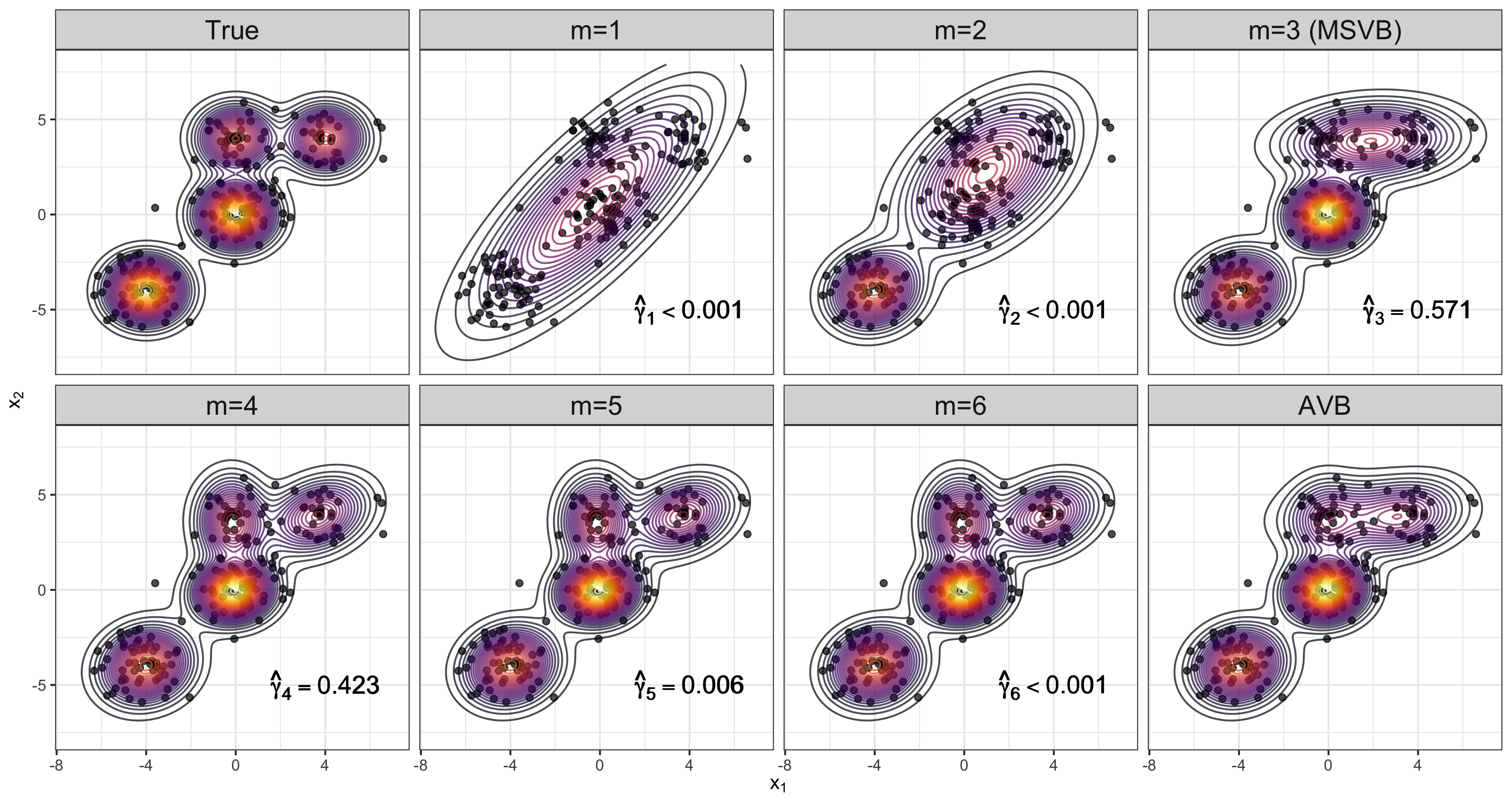
Figure 1: Contour plots for the true and predictive densities.

A.2 Neural network regression

We here compare the predictive abilities of the two variational posteriors over neural networks, computed by the adaptive variational Bayes and the model selection variational Bayes, respectively. We consider the set of network architectures given as $\mathcal{M}_{n}=\{2,3\}\times\{25,50,100\}$. In this experiment, we consider the shallow architectures of depth 2 or 3 considering the following facts. First, the required order for the depth in our theory is $\mathscr{O}(\log n)$, which is far smaller than the order of width $\mathscr{O}(n^{d/(4\beta+2d)})$. Moreover, several previous studies liu2016stein, knoblauch2022optimization chose shallow networks for their numerical experiments with the same data sets we use.

We let the prior probability of the model with depth $K$ and width $M$ be proportional to $\textup{e}^{-\mathfrak{a}_{0}K^{2}M^{2}\log n}$ with $\mathfrak{a}_{0}=10^{-4}$. We train each individual variational posteriors for 2,000 epochs, using the ADAM optimizer kingma2014adam with a learning rate of $10^{-2}$.

The performances of the two variational posteriors are evaluated on eight UCI data sets. For each data set, we split the data set into training (90%) and test (10%) sets randomly 50 times. We compute the posterior mean of the neural network based on 100 network parameters generated from the variational posterior and predictions are made based on the approximately computed posterior mean. We calculate the root mean square error (RMSE) on the test set for each of the 50 splits. Table 1 presents these RMSE values of the two variational posteriors and we see that the proposed adaptive variational posterior outperforms the model selection variational posterior.

Table 1: The average of the RMSEs, with its standard error in the parenthesis, over 50 runs. The best performance is indicated with a bold font for each of the eight benchmark UCI data sets.

Data	$n$	$d$	AVB	MSVB
Boston	506	13	3.807 $\pm$ 1.146	4.008 $\pm$ 1.171
Concrete	1030	8	6.06 $\pm$ 0.512	6.325 $\pm$ 0.562
Energy	768	9	2.039 $\pm$ 0.188	2.139 $\pm$ 0.251
Kin8mn	8192	8	0.093 $\pm$ 0.004	0.093 $\pm$ 0.004
Naval	11934	17	0.009 $\pm$ 0.003	0.009 $\pm$ 0.003
Power	9568	4	4.308 $\pm$ 0.233	4.314 $\pm$ 0.228
Wine	1599	11	0.636 $\pm$ 0.035	0.641 $\pm$ 0.036
Yacht	308	6	2.424 $\pm$ 0.856	2.853 $\pm$ 1.418

Appendix B A general approach for testing construction

In this section, we develop a new method to check the testing condition of Assumption A1, which might be of independent interest. We will frequently use the next lemma in our applications, where we denote by $\mathscr{N}(\zeta,\mathcal{B},\mathscr{d})$ the $\zeta$-covering number of a set $\mathcal{B}$ with respect to a metric $\mathscr{d}$.

Lemma B.1 (Sufficient condition of the testing condition).

Suppose that there exist absolute constants $\rho_{\circ}\in(0,1)$, $\rho_{\blacklozenge}>1$, and $\mathfrak{c}_{2}\geq\mathfrak{c}_{1}>0$ such that

$$\mathfrak{c}_{1}n\mathscr{d}_{n}^{2}(\bm{\lambda}_{0},\bm{\lambda}_{1}) \leq\textsf{{D}}_{\rho_{\circ}}\mathinner{\bigl{(}\textsf{{P}}^{(n)}_{\bm{\lambda}_{0}},\textsf{{P}}^{(n)}_{\bm{\lambda}_{1}}\bigr{)}},$$ (B.1)

$$\textsf{{D}}_{\rho_{\blacklozenge}}\mathinner{\bigl{(}\textsf{{P}}^{(n)}_{\bm{\lambda}_{0}},\textsf{{P}}^{(n)}_{\bm{\lambda}_{1}}\bigr{)}} \leq\mathfrak{c}_{2}n\mathscr{d}_{n}^{2}(\bm{\lambda}_{0},\bm{\lambda}_{1})$$ (B.2)

for any $\bm{\lambda}_{0},\bm{\lambda}_{1}\in\Lambda_{n}$ and any sufficiently large $n\in\mathbbm{N}$. Moreover, assume that for any $u>0$, there exists an absolute constant $\mathfrak{c}_{3}(u)>0$ depending on $u$ such that

$$\sup_{\zeta>\zeta_{n,m}}\log\mathscr{N}\mathinner{\bigl{(}u\zeta,\mathinner{\left\{\bm{\theta}\in\Theta_{n,m}\mathrel{\mathop{\mathchar 58\relax}}\mathscr{d}_{n}(\textsf{{T}}(\bm{\theta}),\bm{\lambda}^{\star})\leq 2\zeta\right\}},\mathscr{d}_{n}\bigr{)}}\leq\mathfrak{c}_{3}(u)n\zeta_{n,m}^{2}$$ (B.3)

for any $\bm{\lambda}^{\star}\in\Lambda_{n}^{\star}$, any $m\in\mathcal{M}_{n}$ and any sufficiently large $n\in\mathbbm{N}$. Then Assumption A1 holds.

Proof B.2.

The proof is deferred to Section J.5.1.

In words, the assumptions B.1 and B.2 require that the two divergences $\textsf{{D}}_{\rho_{\circ}}(\cdot,\cdot)$ and $\textsf{{D}}_{\rho_{\blacklozenge}}(\cdot,\cdot)$ are equivalent, while in general, $\textsf{{D}}_{\rho_{\circ}}(\cdot,\cdot)\leq\textup{KL}(\cdot,\cdot)\leq\textsf{{D}}_{\rho_{\blacklozenge}}(\cdot,\cdot)$ always. This equivalence can hold for a statistical experiment consisting of light-tailed distributions. An useful sufficient condition of B.1 and B.2 is that the log likelihood ratio is a sub-Gamma random variable, which was assumed by han2021oracle under the name of a “local Gaussianity condition”.

Lemma B.3 (Local Gaussian likelihood ratio).

Suppose that there exist absolute constants $\mathfrak{c}_{1}^{\prime}>1$, $\mathfrak{c}_{2}^{\prime}>0$ and $\mathfrak{c}_{3}^{\prime}>0$ such that

$$\frac{1}{\mathfrak{c}_{1}^{\prime}}n\mathscr{d}_{n}^{2}(\bm{\lambda}_{0},\bm{\lambda}_{1})\leq\textup{KL}\mathinner{\bigl{(}\textsf{{P}}^{(n)}_{\bm{\lambda}_{0}},\textsf{{P}}^{(n)}_{\bm{\lambda}_{1}}\bigr{)}}\leq\mathfrak{c}_{1}^{\prime}n\mathscr{d}_{n}^{2}(\bm{\lambda}_{0},\bm{\lambda}_{1})$$

and that

$$\textsf{{P}}_{\bm{\lambda}_{0}}^{(n)}\mathinner{\biggl{[}\textup{e}^{t\mathinner{\Bigl{\{}\log\mathinner{\left(\frac{\textsf{{p}}_{n}(\bm{\lambda}_{0},\mathbf{Y}^{(n)})}{\textsf{{p}}_{n}(\bm{\lambda}_{1},\mathbf{Y}^{(n)})}\right)}-\textup{KL}\mathinner{\bigl{(}\textsf{{P}}^{(n)}_{\bm{\lambda}_{0}},\textsf{{P}}^{(n)}_{\bm{\lambda}_{1}}\bigr{)}}\Bigr{\}}}}\biggr{]}}\leq\textup{e}^{\mathfrak{c}_{2}^{\prime}t^{2}n\mathscr{d}_{n}^{2}(\bm{\lambda}_{0},\bm{\lambda}_{1})}$$

for any $t\in[-\mathfrak{c}_{3}^{\prime},\mathfrak{c}_{3}^{\prime}],$ any $\bm{\lambda}_{0},\bm{\lambda}_{1}\in\Lambda_{n}$ and any sufficiently large $n\in\mathbbm{N}$. Then B.1 and B.2 hold.

Proof B.4.

The proof is deferred to Section J.5.2.

Remark B.5.

With Lemma B.1, we are able to derive a contraction rate of the adaptive variational posterior with respect to the metric $\mathscr{d}_{n}$ that is equivalent to the KL divergence. Though the condition of the lemma is satisfied by a number of examples, such as experiments in Section 4 and Appendix D, and many other examples in han2021oracle, this is limited for dealing with contraction with respect to weaker metrics. For example, the operator norm $\mathinner{\lVert{\bm{\Sigma}}\rVert}_{\textup{op}}\mathrel{\mathop{\mathchar 58\relax}}=\sup_{\mathbf{x}\in\mathbb{R}^{d}\mathrel{\mathop{\mathchar 58\relax}}|\mathbf{x}|_{2}=1}|\bm{\Sigma}\mathbf{x}|_{2}$ which is frequently used for evaluating estimation of a covariance matrix $\bm{\Sigma}^{\star}\in\mathbbm{S}_{++}^{d}$ does not satisfy B.2. Manual construction of a test function is required in such a case. Meanwhile, for the Hellinger or total variation distances that are weaker than the KL divergence, we can directly check the testing condition of Assumption A1 by using some well-known results on testing construction. We refer to Appendix D of ghosal2017fundamentals for details.

Appendix C Remarks on simplifications of the theoretical conditions of Zhang and Gao [2020]

In this section, we give a detailed comparison of our Assumption A with the assumptions of zhang2020convergence. Recall that the original posterior $\Pi_{n,m}(\cdot|\mathbf{Y}^{(n)})$ is written as

$$\textup{d}\Pi_{n,m}(\bm{\theta}|\mathbf{Y}^{(n)})\mathrel{\mathop{\mathchar 58\relax}}=\frac{\textsf{{r}}_{n}(\textsf{{T}}(\bm{\theta}),\bm{\lambda}^{\star})}{D_{n,m}}\textup{d}\Pi_{n,m}(\bm{\theta})\mbox{ with }D_{n,m}\mathrel{\mathop{\mathchar 58\relax}}=\int\textsf{{r}}_{n}(\textsf{{T}}(\bm{\theta}),\bm{\lambda}^{\star})\textup{d}\Pi_{n,m}(\bm{\theta}),$$ (C.1)

where we use the shorthand $\textsf{{r}}_{n}(\textsf{{T}}(\bm{\theta}),\bm{\lambda}^{\star})\mathrel{\mathop{\mathchar 58\relax}}=\textsf{{p}}_{n}(\textsf{{T}}(\bm{\theta}),\mathbf{Y}^{(n)})/\textsf{{p}}_{n}(\bm{\lambda}^{\star},\mathbf{Y}^{(n)})$.

First, we remove the “prior mass” condition typically assumed in posterior contraction analysis. For a detailed explanation, we recall a “traditional” high probability lower bound of the denominator $D_{n,m}$ of the original posterior in C.1 such that

$$\textsf{{P}}_{\bm{\lambda}^{\star}}^{(n)} \mathinner{\left(D_{n,m}\geq\textup{e}^{-T}\Pi_{n,m}\mathinner{\bigl{(}\mathcal{B}_{\textup{KL}}(\bm{\lambda}^{\star},n\epsilon^{2})\bigr{)}}\right)}\geq 1-\frac{2n\epsilon^{2}+1}{T}$$ (C.2)

$$\mbox{ with }\mathcal{B}_{\textup{KL}}(\bm{\lambda}^{\star},n\epsilon^{2})\mathrel{\mathop{\mathchar 58\relax}}=\mathinner{\left\{\bm{\theta}\in\Theta_{n,m}\mathrel{\mathop{\mathchar 58\relax}}\textup{KL}\mathinner{\bigl{(}\textsf{{P}}^{(n)}_{\bm{\lambda}^{\star}},\textsf{{P}}^{(n)}_{\textsf{{T}}(\bm{\theta})}\bigr{)}}\leq n\epsilon^{2}\right\}}$$

for any $T>0$ and $\epsilon>0$ [Lemma 6.26 of Ghosal and Van der Vaart, 2017]. In view of this bound, the prior mass on the KL neighborhood of $\bm{\lambda}^{\star}$ should be sufficiently large to yield a vanishing bound of the posterior probability that we want to control. In this paper, we develop a novel lower bound of $D_{n,m}$, which relies not on the prior mass but on the two quantities in Assumption A2. Indeed, in Lemma J.6 in Section J.3.2, we show that for any $\textit{Q}\in\mathcal{P}(\Theta_{n,m})$ and $T>0$,

$$\textsf{{P}}_{\bm{\lambda}^{\star}}^{(n)}\mathinner{\left(D_{n,m}\geq\textup{e}^{-T-\textup{KL}(\textit{Q},\Pi_{n,m})}\right)}\geq 1-\frac{1}{T}\mathinner{\Bigl{(}2\textit{Q}\mathinner{\bigl{[}\textup{KL}\mathinner{\bigl{(}\textsf{{P}}_{\bm{\lambda}^{\star}}^{(n)},\textsf{{P}}_{\textsf{{T}}(\bm{\theta})}^{(n)}\bigr{)}}\bigr{]}}+1\Bigr{)}}.$$ (C.3)

Thus, under Assumption A2, we get a high probability lower bound of the denominator $D_{n,m}$ with $\textit{Q}=\textit{Q}_{n,m}^{*}$ and large $T>0$ such that $n(\eta_{n,m}+\zeta_{n,m})^{2}/T\to 0$. It is easy to see that the traditional bound in C.2 is recovered when we let $\textit{Q}(\cdot)=\Pi_{n,m}(\cdot|\mathcal{B}_{\textup{KL}}(\bm{\lambda}^{\star},n\epsilon^{2}))$.

Second, we weaken the unnecessarily strong condition on the prior distribution. Zhang and Gao [2020] employed an “overwhelming” probability lower bound of $D_{n,m}$ such that

$$\textsf{{P}}_{\bm{\lambda}^{\star}}^{(n)} \mathinner{\left(D_{n,m}\geq\textup{e}^{-T}\Pi_{n,m}\mathinner{\bigl{(}\mathcal{B}_{\rho}(\bm{\lambda}^{\star},n\epsilon^{2})\bigr{)}}\right)}\geq 1-\exp\mathinner{(-\rho(T-n\epsilon^{2}))},$$

$$\mbox{ with }\mathcal{B}_{\rho}(\bm{\lambda}^{\star},n\epsilon^{2})\mathrel{\mathop{\mathchar 58\relax}}=\mathinner{\left\{\bm{\theta}\in\Theta_{n,m}\mathrel{\mathop{\mathchar 58\relax}}\textsf{{D}}_{\rho}\mathinner{\bigl{(}\textsf{{P}}^{(n)}_{\bm{\lambda}^{\star}},\textsf{{P}}^{(n)}_{\textsf{{T}}(\bm{\theta})}\bigr{)}}\leq n\epsilon^{2}\right\}}$$

for some $\rho>1$, which converges to 1 exponentially in $T>0$, in order to ensure that their PAC-Bayes oracle bound vanishes asymptotically. For this purpose, they assumed that the prior mass on the “smaller” neighborhood $\mathcal{B}_{\rho}(\bm{\lambda}^{\star},n\epsilon^{2})\subset\mathcal{B}_{\textup{KL}}(\bm{\lambda}^{\star},n\epsilon^{2})$ is sufficiently large. We avoid requiring this stronger prior mass condition by slightly modifying the proof so that the polynomially converging probability bound in C.3 can be used.

Appendix D Additional remarks and results on adaptive variational deep learning

D.1 Existing results on nonparametric regression with deep neural networks

In this subsection, we discuss the previous results on the estimation of Hölder smooth regression function with deep neural networks and compare them with our result. Our Corollary 4.3 is the first adaptive optimal one for the non-sparse neural network model. This directly follows from Theorem 4.2 and the function approximation analysis by non-sparse neural networks given in Section K.1.1 which is largely borrowed from kohler2021rate and lu2020deep. Therefore, applying the Bayesian adaptation theory developed by lember2007universal,ghosal2008nonparametric,han2021oracle, one can expect adaptive optimality of an original posterior over non-sparse neural networks with varying depth and width, although this has not been done before. However, posterior computation is not easy since depth and width should be dealt with as random variables. On the frequentist side, kohler2021rate and jiao2023deep showed the optimality of an empirical risk minimizer over non-sparse neural networks. Even though their results are basically non-adaptive since network width and/or depth should be chosen based on the smoothness $\beta$, using a theoretically guaranteed model selection technique such as the training-validation approach [e.g.,][]hamm2021adaptive, the frequentist neural network estimator can be made adaptive without much difficulty.

For sparse neural network models, many studies have constructed optimal estimators, but most of them are non-adaptive in the sense that the network sparsity depends on the smoothness of the true regression function schmidt2020nonparametric, suzuki2018adaptivity, imaizumi2020advantage, kim2021fast. Certain penalization ohn2022nonconvex and hierarchical Bayes polson2018posterior methods can be used to attain sparse neural network estimators that are adaptive to the unknown smoothness. cherief2020convergence proposed an adaptive sparse deep learning method based on the model selection variational Bayes with fractional likelihoods of cherief2019consistency.

D.2 Estimation of composition structured regression functions

To avoid the curse of dimensionality that exists in the convergence rate of estimation of Hölder smooth regression function, one can make a certain structural assumption on the regression function. schmidt2020nonparametric and kohler2021rate considered so-called composition structured regression functions which include a single-index model gaiffas2007optimal, an additive model stone1985additive, buja1989linear and a generalized additive model with an unknown link function horowitz2007rate as particular instances. Under this structure assumption, they derived the improved convergence rates of sparse and non-sparse neural networks respectively, but note again, that their estimators are nonadaptive.

In this subsection, we show that the adaptive variational deep learning enjoys the optimal contraction rate under the composition structure assumption. Recall the definition of the class of composition structured functions considered in schmidt2020nonparametric

$$\mathcal{F}^{\textsc{comp}}\mathinner{\bigl{(}r,(\beta_{\ell})_{\ell\in[r]},(s_{\ell})_{\ell\in[r]},(d_{\ell})_{\ell\in[r]},F_{0}\bigr{)}}$$ (D.1)

$$\mathrel{\mathop{\mathchar 58\relax}}=\mathinner{\left\{f_{r}\circ(f_{r-1,j})_{j\in[d_{r}]}\cdots\circ(f_{1,j})_{j\in[d_{2}]}\in\mathcal{F}^{d_{1}}\mathrel{\mathop{\mathchar 58\relax}}f_{\ell,j}\in\mathcal{H}^{\beta_{\ell},s_{\ell},F_{0}},0\leq f_{\ell,j}\leq 1\right\}}$$

for the number of compositions $r\in\mathbbm{N}$ and the number of intermediate functions $d_{\ell}\in\mathbbm{N}$ (except $d_{1}$ being the input dimension), smoothness $\beta_{\ell}\in\mathbb{R}_{+}$, and intrinsic dimension $s_{\ell}\in[d_{\ell}]$ at the $\ell$-th stage for $\ell\in[r]$. We here assume that the outputs of the functions $\{f_{\ell,j}\mathrel{\mathop{\mathchar 58\relax}}j\in[d_{\ell+1}],\ell\in[r-1])\}$ can be easily generalized to an arbitrary compact subset of the real line, but we do not consider this generalization for technical simplicity.

Corollary D.1 (Composition structured regression function).

Let $r\in\mathbbm{N}$, $\mathbf{d}=(d_{\ell})_{\ell\in[r]}$, $\bm{\beta}\mathrel{\mathop{\mathchar 58\relax}}=(\beta_{\ell})_{\ell\in[r]}\in\mathbb{R}_{+}^{r}$, $\mathbf{s}\mathrel{\mathop{\mathchar 58\relax}}=(s_{\ell})_{\ell\in[r]}\in\otimes_{\ell=1}^{r}[d_{\ell}]$ and $F_{0}>0$. Then under Assumption C, we have

$$\sup_{f^{\star}\in\mathcal{F}^{\textsc{comp}}\mathinner{\left(r,\mathbf{d},\bm{\beta},\mathbf{s},F_{0}\right)}}\textsf{{P}}_{f^{\star}}^{(n)}\mathinner{\left[\widehat{\textit{Q}}_{n}\mathinner{\left(\mathinner{\lVert{\textup{{net}}(\bm{\theta})-f^{\star}}\rVert}_{n,2}\geq\max_{\ell\in[r]}n^{-\frac{\beta_{\geq\ell}}{2\beta_{\geq\ell}+s_{\ell}}}\log^{2}n\right)}\right]}=\mathscr{o}(1),$$ (D.2)

where we let $\beta_{\geq\ell}\mathrel{\mathop{\mathchar 58\relax}}=\beta_{\ell}\prod_{h=\ell+1}^{r}(\beta_{h}\wedge 1)$ for $\ell\in[r-1]$ and $\beta_{\geq r}\mathrel{\mathop{\mathchar 58\relax}}=\beta_{r}$.

Proof D.2.

The proof is deferred to Section K.2.2.

If the intrinsic dimensions $s_{1},\dots,s_{r}$ are much smaller than the input dimension $d_{1}$, the convergence rate improves substantially compared to the rate for the Hölder smooth functions. Also, the contraction rate of the above corollary is minimax optimal [Theorem 3 of][]schmidt2020nonparametric.

Very recently, it was proven that no standard Gaussian process (GP) can attain the minimax optimal contraction rate giordano2022inability, while a deep GP that “stacks” multiple GPs can do finocchio2023posterior for estimating composition structured regression functions. Thus, theoretically, the proposed variational deep learning performs better than any GP and is comparable to the deep GP in this setup. Also, any wavelet estimator only attains a sub-optimal convergence rate schmidt2020nonparametric.

D.3 Binary classification

We consider a statistical experiment of binary classification. Let $\mathbf{Y}\mathrel{\mathop{\mathchar 58\relax}}=(\mathbf{X},Y)\in\mathbbm{Y}\mathrel{\mathop{\mathchar 58\relax}}=[0,1]^{d}\times\{0,1\}$ be a pair of input-label variables such that $\mathbf{X}\sim\texttt{{Unif}}([0,1]^{d})$ and $Y|\mathbf{X}=\mathbf{x}\sim\texttt{{Bernoulli}}(p(\mathbf{x}))$ for some conditional class probability function $p\in\mathcal{F}^{d}_{[\varkappa,1-\varkappa]}\mathrel{\mathop{\mathchar 58\relax}}=\mathinner{\{p\in\mathcal{F}^{d}\mathrel{\mathop{\mathchar 58\relax}}\varkappa\leq p\leq 1-\varkappa\}}$ for $\varkappa\in(0,1/2)$. Here, we assume that the conditional class probability is bounded away from 0 and 1. This is in order to avoid the diverging behavior of the likelihood near 0 or 1. Such an assumption has been commonly made in analyzing logistic models [e.g.,][]van2014asymptotically,ohn2022nonconvex. For each $n\in\mathbbm{N}$, we observe $n$ iid input-label pairs $\mathbf{Y}^{(n)}\mathrel{\mathop{\mathchar 58\relax}}=((\mathbf{X}_{i},Y_{i}))_{i\in[n]}$ which are independently generated from the above probability model, i.e., $\mathbf{Y}^{(n)}\sim\textsf{{P}}_{p}^{(n)}$ for $p\in\mathcal{F}^{d}_{[\varkappa,1-\varkappa]}$, where $\textsf{{P}}_{p}^{(n)}$ is a distribution with the likelihood $\textsf{{p}}_{n}^{\textup{Ber}}(p,\cdot)$ defined as

$$\textsf{{p}}_{n}^{\textup{Ber}}(p,\mathbf{Y}^{(n)})=\prod_{i=1}^{n}\mathinner{\left\{p(\mathbf{X}_{i})^{Y_{i}}\mathinner{\left(1-p(\mathbf{X}_{i})\right)}^{1-Y_{i}}\right\}}.$$ (D.3)

Lemma D.3.

Let $\varkappa\in(0,1/2)$ be an arbitrary small positive number. A sequence of the binary classification experiments $\mathinner{\bigl{(}\mathinner{(\mathbbm{Y}^{\otimes n},\mathcal{P}(\mathbbm{Y}^{\otimes n};\textsf{{p}}_{n}^{\textup{Ber}},\mathcal{F}^{d}_{[\varkappa,1-\varkappa]}))}\bigr{)}}_{n\in\mathbbm{N}}$ satisfies B.1 and B.2 with the metric $\mathscr{d}_{n}\mathrel{\mathop{\mathchar 58\relax}}\mathcal{F}^{d}_{[\varkappa,1-\varkappa]}\times\mathcal{F}^{d}_{[\varkappa,1-\varkappa]}\mapsto\mathbb{R}_{\geq 0}$ defined as $\mathscr{d}_{n}(p_{0},p_{1})=\|p_{0}-p_{1}\|_{2}$ for $p_{0},p_{1}\in\mathcal{F}^{d}_{[\varkappa,1-\varkappa]}$.

Proof D.4.

The proof is deferred to Section K.3.2.

We model $p$ itself by a neural network, i.e., the likelihood of a network parameter $\bm{\theta}$ is given by $\prod_{i=1}^{n}(\textup{{net}}(\bm{\theta})(\mathbf{X}_{i}))^{Y_{i}}(1-\textup{{net}}(\bm{\theta})(\mathbf{X}_{i}))^{1-Y_{i}}$. To ensure that neural network estimates are bounded away from 0 and 1, we use a truncation operator as $\textup{{net}}_{[\varkappa,1-\varkappa]}(\bm{\theta})\mathrel{\mathop{\mathchar 58\relax}}=(\textup{{net}}(\bm{\theta})\vee\varkappa)\wedge(1-\varkappa)$ for a network parameter $\bm{\theta}$.

The following corollary shows that if the true conditional probability function is Hölder $\beta$-smooth, our adaptive variational deep learning is able to estimate it with the optimal rate. The proof is almost similar to the proof of Corollary 4.3, so we omit it.

Corollary D.5 (Hölder smooth conditional class probability).

Let $\beta>0$, $d\in\mathbbm{N}$, $F_{0}>0$ and $\varkappa\in(0,1/2)$. Then under Assumption C, we have

$$\sup_{p^{\star}\in\mathcal{H}^{\beta,d,F_{0}}_{[\varkappa,1-\varkappa]}}\textsf{{P}}_{p^{\star}}^{(n)}\mathinner{\left[\widehat{\textit{Q}}_{n}\mathinner{\left(\left\|{\textup{{net}}_{[\varkappa,1-\varkappa]}(\bm{\theta})-p^{\star}}\right\|_{2}\geq n^{-\frac{\beta}{2\beta+d}}\log^{2}n\right)}\right]}=\mathscr{o}(1),$$ (D.4)

where $\mathcal{H}^{\beta,d,F_{0}}_{[\varkappa,1-\varkappa]}\mathrel{\mathop{\mathchar 58\relax}}=\mathinner{\bigl{\{}p\in\mathcal{H}^{\beta,d,F_{0}}\mathrel{\mathop{\mathchar 58\relax}}\varkappa\leq p\leq 1-\varkappa\bigr{\}}}.$

D.4 Intensity estimation for Poisson point processes

Let $\mathcal{X}$ be the Borel $\sigma$-field of $[0,1]^{d}$. For each $n\in\mathbbm{N}$, we consider a Poisson point process $Y$ on $[0,1]^{d}$ with intensity $\lambda\mathrel{\mathop{\mathchar 58\relax}}[0,1]^{d}\mapsto\mathbb{R}_{\geq 0}$, that is, $Y$ is an integer-valued random measure such that

1. for any $k\in\mathbbm{N}$ and any disjoint $X_{1},\dots,X_{k}\in\mathcal{X}$, the random variables $Y(X_{1}),\dots,Y(X_{k})$ are independent;

2. for any $X\in\mathcal{X}$, $Y(X)\sim\texttt{{Poisson}}\mathinner{\left(\int_{X}\lambda(\mathbf{x})\textup{d}\mathbf{x}\right)}$.

Let $\bar{\mathbbm{Y}}$ be a set of realizations of the Poisson point process $Y$, i.e.,

$$\bar{\mathbbm{Y}}\mathrel{\mathop{\mathchar 58\relax}}=\mathinner{\left\{\sum_{j=1}^{N}\delta(\cdot;\mathbf{x}_{j}^{\prime})\mathrel{\mathop{\mathchar 58\relax}}N\in\mathbbm{N},\mathbf{x}_{j}^{\prime}\in[0,1]^{d}\right\}}.$$

The aim is to recover the intensity function $\lambda$ of the Poisson point process $Y$ based on $n$ independent realizations $\mathbf{Y}^{(n)}\mathrel{\mathop{\mathchar 58\relax}}=(Y_{i})_{i\in[n]}\in\bar{\mathbbm{Y}}^{\otimes n}$ of $Y$. With a reference measure being the Poisson point process with constant intensity $\lambda\equiv 1$, we can consider a likelihood function $\textsf{{p}}_{n}^{\textup{PPP}}\mathrel{\mathop{\mathchar 58\relax}}\mathcal{F}_{\geq 0}^{d}\times\bar{\mathbbm{Y}}^{\otimes n}\mapsto\mathbb{R}_{\geq 0}$ given by

$$\textsf{{p}}_{n}^{\textup{PPP}}(\lambda,\mathbf{Y}^{(n)})=\prod_{j=1}^{n}\exp\mathinner{\left(\int\log\lambda(\mathbf{x})\textup{d}Y_{i}(\mathbf{x})-\int_{[0,1]^{d}}(\lambda(\mathbf{x})-1)\textup{d}\mathbf{x}\right)}\mbox{ for }\lambda\in\mathcal{F}_{\geq 0}^{d},$$ (D.5)

where $\mathcal{F}_{\geq 0}^{d}$ denotes the set of measurable nonnegative functions supported on $[0,1]^{d}$. Let $\textsf{{P}}_{\lambda}^{(n)}$ be a distribution of the Poisson point process $Y$ with the likelihood function $\textsf{{p}}_{n}(\lambda,\cdot)$.

We first check the conditions in Lemma B.1. For this, we assume that every intensity function is bounded away from zero and infinity for technical simplicity. That is, we assume that every intensity belongs to a class $\mathcal{F}^{d}_{[\varkappa_{\min},\varkappa_{\max}]}\mathrel{\mathop{\mathchar 58\relax}}=\mathinner{\{\lambda\in\mathcal{F}^{d}\mathrel{\mathop{\mathchar 58\relax}}\varkappa_{\min}\leq\lambda\leq\varkappa_{\max}\}}$ for given $\varkappa_{\max}>\varkappa_{\min}>0$.

Lemma D.6.

For any $\varkappa_{\max}>\varkappa_{\min}>0$, a sequence of the Poisson point process experiments $\mathinner{\bigl{(}\mathinner{(\bar{\mathbbm{Y}}^{\otimes n},\mathcal{P}(\bar{\mathbbm{Y}}^{\otimes n};\textsf{{p}}_{n}^{\textup{PPP}},\mathcal{F}^{d}_{[\varkappa_{\min},\varkappa_{\max}]}))}\bigr{)}}_{n\in\mathbbm{N}}$ satisfies B.1 and B.2 with the metric $\mathscr{d}_{n}\mathrel{\mathop{\mathchar 58\relax}}\mathcal{F}^{d}_{[\varkappa_{\min},\varkappa_{\max}]}\times\mathcal{F}^{d}_{[\varkappa_{\min},\varkappa_{\max}]}\mapsto\mathbb{R}_{\geq 0}$ defined as $\mathscr{d}_{n}(\lambda_{0},\lambda_{1})=\|\lambda_{0}-\lambda_{1}\|_{2}$ for $\lambda_{0},\lambda_{1}\in\mathcal{F}^{d}_{[\varkappa_{\min},\varkappa_{\max}]}$.

Proof D.7.

The proof is deferred to Section K.3.3.

We directly model $\lambda$ by a neural network in a sense that the likelihood of a network parameter $\bm{\theta}$ is given by $\textsf{{p}}_{n}^{\textup{PPP}}(\textup{{net}}(\bm{\theta}),\mathbf{Y}^{(n)})$. To ensure boundedness of neural network intensity estimates, we apply a truncation operator as $\textup{{net}}_{[\varkappa_{\min},\varkappa_{\max}]}(\bm{\theta})\mathrel{\mathop{\mathchar 58\relax}}=(\textup{{net}}(\bm{\theta})\vee\varkappa_{\min})\wedge\varkappa_{\max}$ for a network parameter $\bm{\theta}$. In the next corollary, we show that the adaptive variational deep learning attains the optimal rate for estimating Hölder $\beta$-smooth intensity functions kutoyants2012statistical. The proof is almost similar to the proof of Corollary 4.3, thus we omit it.

Corollary D.8 (Hölder smooth intensity).

Let $\beta>0$, $d\in\mathbbm{N}$, $F_{0}>0$ and $\varkappa_{\max}>\varkappa_{\min}>0$. Then under Assumption C, we have

$$\sup_{\lambda^{\star}\in\mathcal{H}^{\beta,d,F_{0}}_{[\varkappa_{\min},\varkappa_{\max}]}}\textsf{{P}}_{\lambda^{\star}}^{(n)}\mathinner{\biggl{[}\widehat{\textit{Q}}_{n}\mathinner{\left(\left\|{\textup{{net}}_{[\varkappa_{\min},\varkappa_{\max}]}(\bm{\theta})-\lambda^{\star}}\right\|_{2}\geq n^{-\frac{\beta}{2\beta+d}}\log^{2}n\right)}\biggr{]}}=\mathscr{o}(1),$$ (D.6)

where $\mathcal{H}^{\beta,d,F_{0}}_{[\varkappa_{\min},\varkappa_{\max}]}\mathrel{\mathop{\mathchar 58\relax}}=\mathinner{\bigl{\{}\lambda\in\mathcal{H}^{\beta,d,F_{0}}\mathrel{\mathop{\mathchar 58\relax}}\varkappa_{\min}\leq\lambda\leq\varkappa_{\max}\bigr{\}}}.$

Appendix E Computation algorithm and simulation study for sparse factor models

In this section, we carry out a simulation study to evaluate the performance of the adaptive variational Bayes method on sparse factor models, which was considered in Section 5.2.

E.1 The PX-CAVI algorithm

We present the parameter expansion coordinate-ascent variational inference (PX-CAVI) algorithm proposed by ning2021spike for computing the variational posterior over each individual factor model with fixed factor dimensionality, say $m$, based on the spike-and-slab prior distribution

$$\Pi_{n,m}\mathrel{\mathop{\mathchar 58\relax}}=\mathinner{\left\{(1-\omega_{m})\delta(\cdot;\mathbf{0}_{m})+\omega_{m}\texttt{{N}}(\mathbf{0}_{m},\tau_{0}\mathbf{I}_{m})\right\}}^{\otimes d}\text{ with }\omega_{m}\mathrel{\mathop{\mathchar 58\relax}}=d^{-(1+\mathfrak{a}_{0})m}$$

and the spike-and-slab variational family

$$\mathcal{Q}_{n,m}\mathrel{\mathop{\mathchar 58\relax}}=\mathinner{\left\{\bigotimes_{j=1}^{d}\mathinner{\left\{(1-\nu_{j})\delta(\cdot;\mathbf{0}_{m})+\nu_{j}\texttt{{N}}(\bm{\psi}_{j},\bm{\Phi}_{j})\right\}}\mathrel{\mathop{\mathchar 58\relax}}\bm{\psi}_{j}\in\mathbb{R}^{m},\bm{\Phi}_{j}\in\mathbbm{S}_{++}^{m},\nu_{j}\in[0,1]\right\}}.$$

Here and in the rest of the section, we write $d=d_{n}$ and $\omega_{m}=\omega_{n,m}$ for convenience.

Following ning2021spike, we introduce latent variables $(\mathbf{x}_{i})_{i\in[n]}\in(\mathbb{R}^{m})^{\otimes n}$ and employ the parameter expansion technique. Then we can write the sparse factor model as

$$\mathbf{Y}_{i}|\mathbf{x}_{i}\stackrel{{\scriptstyle\textup{ind}}}{{\sim}}\texttt{{N}}(\mathbf{L}\mathbf{K}\mathbf{x}_{i},\mathbf{I}_{d}),\quad\mathbf{x}_{i}\stackrel{{\scriptstyle\textup{iid}}}{{\sim}}\texttt{{N}}\mathinner{\bigl{(}\mathbf{0}_{m},(\mathbf{K}\mathbf{K}^{\top})^{-1}\bigr{)}}$$

for $i\in[n]$, where $\mathbf{K}\in\mathbb{R}^{m\times m}$ is a lower triangular matrix that will be updated in the algorithm. We consider a normal variational distribution $\bigotimes_{i=1}^{n}\texttt{{N}}(\mathbf{b}_{i},\mathbf{V})$ for the latent variables $(\mathbf{x}_{i})_{i\in[n]}$, and we estimate $(\mathbf{b}_{i})_{i\in[n]}\in(\mathbb{R}^{m})^{\otimes n}$ and $\mathbf{V}\in\mathbbm{S}_{++}^{m}$. At every iteration of the algorithm, the following component-wise updates are conducted.

• (Update $\widehat{\bm{\psi}}_{j}$ and $\widehat{\bm{\Phi}}_{j}$) Calculate

  $$\bar{\mathbf{H}}^{[t+1]}\mathrel{\mathop{\mathchar 58\relax}}=\frac{1}{n}\sum_{i=1}^{n}\mathbf{H}_{i}^{[t+1]}\text{ with }\mathbf{H}_{i}^{[t+1]}\mathrel{\mathop{\mathchar 58\relax}}=\mathbf{K}^{[t]}\mathinner{\bigl{\{}\mathbf{b}_{i}^{[t]}(\mathbf{b}_{i}^{[t]})^{\top}+\mathbf{V}^{[t]}\bigr{\}}}(\mathbf{K}^{[t]})^{\top}$$

  and then calculate

  $$\bm{\Phi}_{j}^{[t+1]} \mathrel{\mathop{\mathchar 58\relax}}=\bm{\Phi}^{[t+1]}\mathrel{\mathop{\mathchar 58\relax}}=\mathinner{\bigl{(}n\bar{\mathbf{H}}^{[t+1]}+\tau_{0}\mathbf{I}_{m}\bigr{)}}^{-1},$$

  $$\bm{\psi}_{j}^{[t+1]} \mathrel{\mathop{\mathchar 58\relax}}=\bm{\Phi}^{[t+1]}\sum_{i=1}^{n}Y_{ij}\mathbf{K}^{[t]}\mathbf{b}_{i}^{[t]}$$

  for each $j\in[d]$, where $Y_{ij}$ denotes the $j$-th element of $\mathbf{Y}_{i}$ for $i\in[n]$.

• (Update $\nu_{j}$) Let $\text{lgst}(z)=\textup{e}^{z}/(1+\textup{e}^{z})$ for $z\in\mathbb{R}$. For each $j\in[d]$, calculate

  $$\nu_{j}^{[t+1]}\mathrel{\mathop{\mathchar 58\relax}}=\text{lgst}\mathinner{\biggl{(}\log\frac{\omega_{m}}{1-\omega_{m}}-B_{j}^{[t+1]}-\frac{1}{2}\sum_{i=1}^{n}E_{ij}^{[t+1]}\biggr{)}},$$

  where we define

  $$E_{ij}^{[t+1]}\mathrel{\mathop{\mathchar 58\relax}}=-2Y_{ij}(\mathbf{K}^{[t]}\mathbf{b}_{i}^{[t]})^{\top}\bm{\psi}_{j}^{[t+1]}+(\bm{\psi}_{j}^{[t+1]})^{\top}\mathbf{H}_{i}^{[t+1]}\bm{\psi}_{j}^{[t+1]}+\Tr\mathinner{\bigl{(}\bm{\Phi}^{[t+1]}\mathbf{H}_{i}^{[t+1]}\bigr{)}}$$

  and we denote by $B_{j}^{[t+1]}$ the KL divergence from the prior $\texttt{{N}}(\mathbf{0}_{m},\tau_{0}\mathbf{I}_{m})$ to the variational distribution $\texttt{{N}}(\bm{\psi}_{j}^{[t+1]},\bm{\Phi}_{j}^{[t+1]})$ for the parameter $\mathbf{L}_{j,\mathrel{\mathop{\mathchar 58\relax}}}$, that is,

  $$B_{j}^{[t+1]}\mathrel{\mathop{\mathchar 58\relax}}=-\frac{m}{2}+\frac{1}{2}\log\mathinner{\biggl{(}\frac{|\tau_{0}\mathbf{I}_{m}|}{\mathinner{\lvert\bm{\Phi}^{[t+1]}\rvert}}\biggr{)}}-\frac{1}{2\tau_{0}}\mathinner{\Bigl{\{}(\bm{\psi}_{j}^{[t+1]})^{\top}\bm{\psi}_{j}^{[t+1]}+\Tr\mathinner{\bigl{(}\bm{\Phi}^{[t+1]}\bigr{)}}\Bigr{\}}}.$$

• (Update $\mathbf{b}_{i}$ and $\mathbf{V}$) Calculate

  $$\mathbf{V}^{[t+1]} \mathrel{\mathop{\mathchar 58\relax}}=\mathinner{\biggl{(}\sum_{j=1}^{d}\nu_{j}^{[t+1]}(\mathbf{K}^{[t]})^{\top}\mathinner{\bigl{\{}\bm{\psi}_{j}^{[t+1]}(\bm{\psi}_{j}^{[t+1]})^{\top}+\bm{\Phi}^{[t+1]}\bigr{\}}}\mathbf{K}^{[t]}+\mathbf{I}_{m}\biggr{)}}^{-1},$$

  $$\mathbf{b}_{i}^{[t+1]} \mathrel{\mathop{\mathchar 58\relax}}=\mathbf{V}^{[t+1]}\sum_{j=1}^{d}Y_{ij}\nu_{j}^{[t]}(\bm{\psi}_{j}^{[t+1]})^{\top}\mathbf{K}^{[t]}$$

  for each $i\in[n]$.

• (Update $\mathbf{K}$) Let $\mathbf{K}^{[t+1]}$ be a lower triangular matrix satisfying

  $$\mathbf{K}^{[t+1]}(\mathbf{K}^{[t+1]})^{\top}=\mathinner{\biggl{(}\frac{1}{n}\sum_{i=1}^{n}\mathbf{b}_{i}^{[t+1]}(\mathbf{b}_{i}^{[t+1]})^{\top}+\mathbf{V}^{[t+1]}\biggr{)}}^{-1},$$

  i.e., $\mathbf{K}^{[t+1]}$ is the lower Cholesky factor of the matrix in the right-hand side of the preceding display.

E.2 Simulation study

We empirically compare the performance of the adaptive variational Bayes (AVB) and other existing methods for covariance matrix estimation. We fix the hyperparameters of the prior as $\mathfrak{a}_{0}=0.01$ and $\tau_{0}=100$ and consider the model space $\mathcal{M}=[10]$ for the factor dimensionality $m$. We use the variational posterior mean of the covariance matrix as a point estimator produced by the adaptive variational Bayes. For competitors, we consider the principal orthogonal complement thresholding method (POET, fan2013large), and two maximum a posteriori estimators that employ the multi-scale generalized double Pareto prior (MDP, srivastava2017expandable) and the spike-and-slab lasso with Indian buffet process prior (SSL-IBP, rovckova2016fast), respectively. For the POET method, the factor dimensionality must be chosen before its estimation, and we use the true factor dimensionality for this.

A synthetic sample of size $n=200$ is generated from the $d=1000$-dimensional normal distribution with mean $\mathbf{0}$ and covariance $\bm{\Sigma}^{\star}\mathrel{\mathop{\mathchar 58\relax}}=\mathbf{L}^{\star}(\mathbf{L}^{\star})^{\top}+\mathbf{I}$, where the true loading matrix $\mathbf{L}^{\star}\in\mathbb{R}^{d\times r}$ has $s$ many nonzero rows. We generate the true loading matrix $\mathbf{L}^{\star}$ as follows: we first select positions of $s$ nonzero rows and sample the elements in each nonzero row from the normal distribution with mean $\mathbf{0}_{r}$ and variance $(5/\sqrt{s})^{2}\mathbf{I}_{r}$. We consider various values of the row sparsity $s\in\{20,50,100\}$ and various values of the factor dimensionality $r\in\{1,3,6\}$. We generate 100 synthetic data sets and we report the averages of the scaled operator norm losses $\mathinner{\lVert{\hat{\bm{\Sigma}}-\bm{\Sigma}^{\star}}\rVert}_{\textup{op}}/\mathinner{\lVert{\bm{\Sigma}^{\star}}\rVert}_{\textup{op}}$ for an estimate $\hat{\bm{\Sigma}}$ and the true covariance matrix $\bm{\Sigma}^{\star}$ computed on the generated synthetic data sets. The result is presented in Table 2 and we can see that the proposed method performs well compared to the other methods.

Table 2: The average of the scaled operator norm losses, and its standard error in the parenthesis, computed on 100 synthetic data sets with $n=200$ and $d=1000$. The best performance is indicated with a bold font for each of the nine considered settings.

$s$	$r$	POET	MDP	SSL-IBP	AVB
20	1	0.563 (0.173)	0.534 (0.163)	0.296 (0.088)	0.144 (0.062)
	3	0.492 (0.151)	0.473 (0.145)	0.285 (0.083)	0.161 (0.072)
	6	0.409 (0.119)	0.397 (0.115)	0.281 (0.077)	0.155 (0.061)
50	1	0.549 (0.205)	0.52 (0.193)	0.286 (0.105)	0.2 (0.077)
	3	0.496 (0.186)	0.473 (0.177)	0.297 (0.119)	0.206 (0.086)
	6	0.468 (0.177)	0.451 (0.171)	0.323 (0.117)	0.216 (0.091)
100	1	0.558 (0.203)	0.526 (0.192)	0.32 (0.117)	0.301 (0.112)
	3	0.533 (0.195)	0.508 (0.186)	0.319 (0.123)	0.323 (0.124)
	6	0.523 (0.196)	0.501 (0.188)	0.362 (0.132)	0.36 (0.144)

Appendix F Application to high-dimensional nonparametric regression using neural networks

In this section, we consider the nonparametric regression experiment considered in Section 4.2, but we allow the input dimension to diverge, which we denoted by $d_{n}$. We assume that the true regression function is a Hölder smooth function that only depends on $s_{0}$ elements in the $d_{n}$-dimensional input, that is, for any $\mathbf{x}\mathrel{\mathop{\mathchar 58\relax}}=(x_{j})_{j\in[d_{n}]}\in[0,1]^{d_{n}}$, $f^{\star}(\mathbf{x})=f_{0}^{\star}((x_{j})_{j\in S^{\star}})$ for some $S^{\star}\subset[d_{n}]$ with $|S^{\star}|=s_{0}$ and $f_{0}^{\star}\in\mathcal{H}^{\beta,s_{0},F_{0}}$. We let $\mathcal{F}^{\textup{sparse}}\mathinner{\left(d_{n},\beta,s_{0},F_{0}\right)}$ be a set of these $s_{0}$-sparse Hölder $\beta$-smooth functions on $[0,1]^{d_{n}}$.

Our aim is to show that the adaptive deep learning achieves the optimal contraction rate to the true regression function $f^{\star}$, and this rate is adaptive simultaneously to the smoothness $\beta$ and the sparsity $s_{0}$. As we did in Section 4.2, we consider multiple network parameter spaces $\{\Theta_{(K,M)}^{d_{n},\leq B_{n}}\}_{(K,M)\in\mathcal{M}_{n}}$ with various network architectures to adapt the smoothness, where $\Theta_{(K,M)}^{d_{n},\leq B_{n}}$ is the set of network parameters with input dimension $d_{n}$, depth $K$, width $M$ and a magnitude bound $B_{n}$ as defined in 4.2. Let $J_{n,(K,M)}\mathrel{\mathop{\mathchar 58\relax}}=(d_{n}+1)M+(K-2)(M^{2}+M)+(M+1)$ be the dimension of the parameter space $\Theta_{(K,M)}^{d_{n},\leq B_{n}}$.

To appropriately address the sparse structure of the true regression function, we impose a spike-and-slab prior on the weight matrix at the first layer. For a network parameter $\bm{\theta}\mathrel{\mathop{\mathchar 58\relax}}=((\mathbf{W}_{k},\mathbf{b}_{k}))_{k\in[K]}\in\Theta_{(K,M)}^{d_{n},\leq B_{n}}$, let $\mathbf{W}_{1,j,\mathrel{\mathop{\mathchar 58\relax}}}\in\mathbb{R}^{M}$ be the $j$-th row of the weight matrix $\mathbf{W}_{1}\in\mathbb{R}^{M\times d_{n}}$ at the first layer. We impose the prior distribution given as

$$\SS_{n,(K,M)}\mathrel{\mathop{\mathchar 58\relax}}=(1-\omega_{n,(K,M)} )\delta(\cdot;\mathbf{0}_{M})+\omega_{n,(K,M)}\texttt{{Unif}}(-B_{n},B_{n})^{\otimes M}\in\mathcal{P}(\mathbb{R}^{M})$$ (F.1)

$$\mbox{ with }\omega_{n,(K,M)}\mathrel{\mathop{\mathchar 58\relax}}=\exp\mathinner{\left(-\mathfrak{a}_{1}KM\log n-(1+\mathfrak{a}_{2})\log d_{n}\right)}$$

on each $\mathbf{W}_{1,j,\mathrel{\mathop{\mathchar 58\relax}}}$, for some arbitrary constants $\mathfrak{a}_{1}>0$ and $\mathfrak{a}_{2}>0$. In words, under the above prior, the event $\{\mathbf{W}_{1,j,\mathrel{\mathop{\mathchar 58\relax}}}=\mathbf{0}\}$ happens with probability $1-\omega_{n,(K,M)}$, and given this event, $x_{j}$ does not affect the output of the neural network. A novel feature of our prior is that the degree of sparse regularization depends on the neural network’s depth and width, enabling us to attain optimality adaptive to both the unknown smoothness and sparsity. We impose an uniform prior distribution on the network parameter’s other elements. To sum up, the prior distribution we assume is

$$\Pi_{n} =\sum_{(K,M)\in\mathcal{M}_{n}}\alpha_{n,(K,M)}\Pi_{n,(K,M)},$$ (F.2)

$$\mbox{ where }\Pi_{n,(K,M)}\mathrel{\mathop{\mathchar 58\relax}}=\mathinner{\bigl{(}\SS_{n,(K,M)}\bigr{)}}^{\otimes d_{n}}\times\texttt{{Unif}}(-B_{n},B_{n})^{\otimes(J_{n,(K,M)}-d_{n}M)}$$

$$\mbox{ and }\alpha_{n,(K,M)}\mathrel{\mathop{\mathchar 58\relax}}=\frac{\textup{e}^{-\mathfrak{a}_{3}(KM)^{2}\log n}}{\sum_{(K^{\prime},M^{\prime})\in\mathcal{M}_{n}}\textup{e}^{-\mathfrak{a}_{3}(K^{\prime}M^{\prime})^{2}\log n}}$$

for some arbitrary constant $\mathfrak{a}_{3}>0$ such that $\mathfrak{a}_{3}>\mathfrak{a}_{1}\wedge\mathfrak{a}_{2}$, where $\mathfrak{a}_{1}>0$ and $\mathfrak{a}_{2}>0$ are the hyperparameters of the spike-and-slab prior in F.1. For each network architecture $(K,M)\in\mathcal{M}_{n}$, we consider a variational family such as

$$\mathcal{Q}_{n,(K,M)}\mathrel{\mathop{\mathchar 58\relax}}=\bigg{\{}\bigotimes_{h=1}^{d_{n}} \mathinner{\Bigl{\{}(1-\nu_{h})\delta(\cdot;\mathbf{0}_{M})+\nu_{h}{{\otimes}}_{j=(h-1)M+1}^{hM}\texttt{{Unif}}(-\psi_{1,j},\psi_{2,j})\Bigr{\}}}$$

$$\times\bigotimes_{j=d_{n}M+1}^{J_{n,(K,M)}}\texttt{{Unif}}(-\psi_{1,j},\psi_{2,j})\mathrel{\mathop{\mathchar 58\relax}}-B_{n}\leq\psi_{1,j}<\psi_{2,j}\leq B_{n},\nu_{h}\in[0,1]\bigg{\}}.$$

The adaptive variational posterior with the above prior and variational families achieves the optimal rate.

Theorem F.1 (Sparse Hölder smooth regression function).

Let $(d_{n})_{n\in\mathbbm{N}}\subset\mathbbm{N}$, $\beta>0$, $s_{0}\in\mathbbm{N}$ and $F_{0}>0$. Assume $s_{0}\leq d_{n}$ eventually. Then under Assumption C, we have

$$\sup_{f^{\star}\in\mathcal{F}^{\textup{sparse}}\mathinner{\left(d_{n},\beta,s_{0},F_{0}\right)}}\textsf{{P}}_{f^{\star}}^{(n)}\mathinner{\left[\widehat{\textit{Q}}_{n}\mathinner{\left(\mathinner{\lVert{\textup{{net}}(\bm{\theta})-f^{\star}}\rVert}_{n,2}\geq n^{-\frac{\beta}{2\beta+s_{0}}}\log^{2}n+A_{n}\sqrt{\frac{\log d_{n}}{n}}\right)}\right]}=\mathscr{o}(1),$$ (F.3)

for any diverging sequence $(A_{n})_{n\in\mathbbm{N}}\to\infty$.

Proof F.2.

The proof is deferred to Section L.3.1.

The contraction rate in the above theorem is optimal up to a logarithmic factor [Yang and Tokdar, 2015]. Yang and Tokdar [2015] and Jiang and Tokdar [2021] showed that Gaussian processes combined with sparsity-inducing priors attain the optimal contraction rate. Another optimal Bayesian approach is Bayesian trees (and their ensembles) with the “spike-and-tree” prior developed by Ročková and van der Pas [2020], but their theoretical analysis is limited to the cases that $0<\beta\leq 1$.

If $\log d_{n}/n=\mathscr{o}(1)$, that is, the dimension diverges slower than the exponential of the sample size, then the contraction rate is the same as the minimax rate $n^{-\beta/({2\beta+s_{0}})}$ for “low”-dimensional nonparametric regression with $s_{0}$-dimensional inputs.

Appendix G Application to a Gaussian sequence model

As a fully nonparametric example, we consider the Gaussian sequence model

$$Y_{i}=\theta_{i}+\frac{1}{\sqrt{n}}Z_{i},\quad Z_{i}\stackrel{{\scriptstyle\textup{iid}}}{{\sim}}\texttt{{N}}(0,1),\quad\text{ for }i\in\mathbbm{N},$$

which is equivalent to the prototypical white noise model $\textup{d}Y(t)=\theta(t)+n^{-1/2}\textup{d}W(t)$ for $t\in[0,1]$ with $\theta\mathrel{\mathop{\mathchar 58\relax}}[0,1]\mapsto\mathbb{R}$ being $\mathscr{L}^{2}$-integrable and $W$ a standard Brownian motion le1986asymptotic. We let $\textsf{{P}}_{\bm{\theta}}^{(n)}\mathrel{\mathop{\mathchar 58\relax}}=\otimes_{i=1}^{\infty}\texttt{{N}}(\theta_{i},n^{-1})$ denote the distribution above. We assume that the true parameter $\bm{\theta}^{\star}\in\mathbb{R}^{\infty}$ belongs to the $\beta$-Sobolev ball

$$\Theta^{\star}=\Theta_{\beta}(B)\mathrel{\mathop{\mathchar 58\relax}}=\mathinner{\left\{\bm{\theta}=(\theta_{i})_{i\in\mathbbm{N}}\mathrel{\mathop{\mathchar 58\relax}}\sum_{i=1}^{\infty}i^{2\beta}\theta_{i}^{2}\leq B^{2}\right\}}$$

for given smoothness $\beta>0$ and radius $B>0$. We will show that the adaptive variational Bayes can attain the minimax optimal rate $n^{-\beta/(2\beta+1)}$ (up to a logarithmic factor) for estimating the true parameter $\bm{\theta}^{\star}\in\Theta_{\beta}(B)$ adaptively in terms of the $\mathscr{L}^{2}$ distance $\mathscr{d}_{n}(\bm{\theta},\bm{\theta}^{\star})=\mathinner{\lvert\bm{\theta}-\bm{\theta}^{\star}\rvert}_{2}$. We consider the set of models $\{\Theta_{n,m}\mathrel{\mathop{\mathchar 58\relax}}=\mathbb{R}^{m}\mathrel{\mathop{\mathchar 58\relax}}m\in\mathcal{M}_{n}\}$, where the model space is given by

$$\mathcal{M}_{n}\mathrel{\mathop{\mathchar 58\relax}}=\mathinner{\left\{\left\lceil{\mathinner{\left(\frac{n}{\log n}\right)}^{k/\log n}}\right\rceil\mathrel{\mathop{\mathchar 58\relax}}k\in\mathinner{\left[\left\lceil{\log n}\right\rceil\right]}\right\}}.$$

On each model $\Theta_{n,m}$ we impose a standard Gaussian prior $\Pi_{n,m}\mathrel{\mathop{\mathchar 58\relax}}=\otimes_{i=1}^{m}\texttt{{N}}(0,1)$. Let T be a natural parametrization map such that $\textsf{{T}}(\bm{\theta})=(\bm{\theta}^{\top},\mathbf{0}_{\infty}^{\top})^{\top}\in\mathbb{R}^{\infty}$, which maps any finite sequence to an infinite one by padding zeros.

In the next two examples, we see how prior regularization, which is a standard method, and ivB regularization, which is proposed in Section 6, are applied in this setup, respectively.

G.1 Prior regularization

Here we consider a variational family

$$\mathcal{Q}_{n,m}\mathrel{\mathop{\mathchar 58\relax}}=\mathinner{\left\{\bigotimes_{i=1}^{m}\texttt{{N}}(\psi_{i},\Phi_{i})\mathrel{\mathop{\mathchar 58\relax}}\psi_{i}\in\mathbb{R},\Phi_{i}>0\right\}}$$

for each $m\in\mathcal{M}_{n}$. Assumption A2 can be verified with $\zeta_{n,m}=m\sqrt{\log n/n}$ and $\eta_{n,m}=Bm^{-\beta}$ as follows: letting $Q_{n,m}^{*}\mathrel{\mathop{\mathchar 58\relax}}=\otimes_{i=1}^{m}\texttt{{N}}(\theta_{i}^{\star},n^{-1})\in\mathcal{Q}_{n,m}$, we have

$$\int\textup{KL}(\textsf{{P}}_{\bm{\theta}^{\star}}^{(n)},\textsf{{P}}_{\textsf{{T}}(\bm{\theta})}^{(n)})\textup{d}Q_{n,m}^{*}(\bm{\theta}) =\frac{n}{2}\int\mathinner{\!\left\lvert\textsf{{T}}(\bm{\theta})-\bm{\theta}^{\star}\right\rvert}_{2}^{2}\textup{d}Q_{n,m}^{*}(\bm{\theta})$$

$$=\frac{m}{2}+\frac{n}{2}\sum_{i=m+1}^{\infty}(\theta^{\star}_{i})^{2}\leq\frac{1}{2}\mathinner{\left(m+nm^{-2\beta}B^{2}\right)}.$$

and

$$\textup{KL}(Q_{n,m}^{*},\Pi_{n,m}) =\frac{1}{2}\mathinner{\left\{m\log n+\frac{m}{n}+\sum_{i=1}^{m}(\theta^{\star}_{i})^{2}-m\right\}}\lesssim m\log n.$$

Moreover, we set the prior model probabilities as $\alpha_{n,m}\propto\exp(-\mathfrak{a}_{0}m\log n)$ for $\mathfrak{a}_{0}>0$ for any $m\in\mathcal{M}_{n}$ which satisfies Assumptions B2 and B3 by Lemma 3.2. Since Assumption A1 is met by Lemma B.7 of zhang2020convergence, we get a contraction rate $\epsilon_{n}$ given by

$$\epsilon_{n}=\min_{m\in\mathcal{M}_{n}}\mathinner{\left\{\sqrt{\frac{m\log n}{n}}+m^{-\beta}\right\}}\asymp\mathinner{\left(\frac{\log n}{n}\right)}^{\beta/(2\beta+1)}.$$

G.2 ivB regularization

In this subsection, we do not use the complexity prior $\alpha_{n,m}\propto\exp(-\mathfrak{a}_{0}m\log n)$ considered above for regularizing overly complex models. Instead, we consider a “constrained” variational family given below to employ the regularization effect of variational approximation. Concretely, we consider

$$\mathcal{Q}_{n,m}^{\dagger}\mathrel{\mathop{\mathchar 58\relax}}=\mathinner{\left\{\bigotimes_{i=1}^{m}\texttt{{N}}(\psi_{i},\Phi_{i})\in\mathcal{Q}_{n,m}\mathrel{\mathop{\mathchar 58\relax}}\sum_{i=1}^{m}(\psi_{i}^{2}+\Phi_{i})\leq B^{2}+1\right\}}.$$ (G.1)

But the variational distribution $Q_{n,m}^{*}\mathrel{\mathop{\mathchar 58\relax}}=\otimes_{i=1}^{m}\texttt{{N}}(\theta_{i}^{\star},n^{-1})$ we used before for checking Assumption A2 is still in $\mathcal{Q}_{n,m}^{\dagger}$ since $\sum_{i=1}^{m}\{(\theta_{i}^{\star})^{2}+n^{-1}\}\leq\sum_{i=1}^{m}i^{2\beta}(\theta_{i}^{\star})^{2}+1\leq B^{2}+1$. This implies that Assumption A2 holds also for the constrained variational family $\mathcal{Q}_{n,m}^{\dagger}$. On the other hand, letting $\Pi_{n,m}^{*}=\texttt{{N}}(0,1/2)^{\otimes m}$, we have that each ivB penalty is lower bounded as

$$\Psi_{n,m} \geq\inf_{\textit{Q}\in\mathcal{Q}_{n,m}^{\dagger}}\mathinner{\left\{\textup{KL}(\textit{Q},\Pi_{n,m})-\textup{KL}(\textit{Q},\Pi_{n,m}^{*})\right\}}$$

$$=\inf_{(\psi_{i},\Phi_{i})_{i\in[m]}\in(\mathbb{R}\times\mathbb{R}_{+})^{\otimes m}\mathrel{\mathop{\mathchar 58\relax}}\sum_{i=1}^{m}(\psi_{i}^{2}+\Phi_{i})\leq B^{2}+1}\mathinner{\left\{\frac{m}{2}\log 2-\frac{1}{2}\sum_{i=1}^{m}(\psi_{i}^{2}+\Phi_{i})\right\}}$$

$$\geq\frac{m}{2}\log 2-\frac{1}{2}(B^{2}+1).$$

Therefore, for any diverging sequence $(A_{n})_{n\in\mathbbm{N}}$, a contraction rate is given by

$$\zeta_{n}^{\ddagger}=\max_{m\in\mathcal{M}_{n}\mathrel{\mathop{\mathchar 58\relax}}\Psi_{n,m}<A_{n}n\epsilon_{n}^{2}}\zeta_{n,m} \leq\max_{m\in\mathcal{M}_{n}\mathrel{\mathop{\mathchar 58\relax}}m<2n\epsilon_{n}^{2}+(B^{2}+1)/2}\zeta_{n,m}$$

$$\lesssim\sqrt{(A_{n}n\epsilon_{n}^{2}+B^{2})\frac{\log n}{n}}$$

$$\lesssim\sqrt{A_{n}}\epsilon_{n}\sqrt{\log n}=\sqrt{A_{n}}n^{-\beta/(2\beta+1)}(\log n)^{(2\beta+1/2)/(2\beta+1)},$$

which is $\sqrt{\log n}$ times larger than the rate $A_{n}\epsilon_{n}$ we obtained using prior regularization.

G.3 Simulation study

We conduct a simulation study to illustrate the performance of the adaptive variational Bayes for the mean estimation of the Gaussian sequence model. For given smoothness $\beta>0$, we generate the true sequence $\bm{\theta}^{\star}$ as $\theta_{i}^{\star}=5s_{i}i^{-\beta-0.6}$ with each $s_{i}$ randomly chosen as $-1$ or 1 with equal probabilities. Then the generated sequence belongs to $\Theta_{\beta}(B)$ with $B=5(\sum_{i=1}^{\infty}i^{-1.2})^{1/2}\leq 12.$ In the simulation, we consider three values 0.5, 1, and 1.5 of $\beta$. For the sample size $n$, we consider $10^{2}$, $10^{3}$, and $10^{4}$.

We consider two adaptive variational Bayes methods, each of which was considered in the previous two sections, respectively. For the prior regularized method (AVBp), we use the prior model probabilities such that $\alpha_{n,m}\propto\exp(-\mathfrak{a}_{0}m\log n)$ with $\mathfrak{a}_{0}=0.1$. For the ivB regularized method (AVBi), we use the uniform prior model probabilities, $\alpha_{n,m}=1/|\mathcal{M}_{n}|$ but restricted variational families $\mathcal{Q}_{n,m}^{\dagger}$ given in G.1 with $B=12$ for every $m\in\mathcal{M}_{n}$. For competitors, we first consider the Bayesian method using the rescaled Gaussian prior (RGP) $\theta_{i}\stackrel{{\scriptstyle\textup{ind}}}{{\sim}}\texttt{{N}}(0,i^{-2\beta_{0}-1})$ with the oracle choice $\beta_{0}=\beta$. This is a non-adaptive but minimax optimal estimator zhao2000bayesian. Another competitor we consider is the mean-field variational Bayes (MFVB) estimator with prior on the truncation level $m$, which was developed and shown to be adaptively optimal by zhang2020convergence. For the MFVB method, we impose the prior distribution $\Pi(m)\propto\exp(-0.1m\log n)$ and $\theta_{1},\dots,\theta_{m}|m\stackrel{{\scriptstyle\textup{iid}}}{{\sim}}\texttt{{N}}(0,1)$, which is the same as the prior we use for the adaptive variational Bayes methods.

We run the simulation 100 times, and, for each method, we compute the square of the $\mathscr{L}^{2}$ distance between the (variational) posterior mean of $\bm{\theta}$ and the true value $\bm{\theta}^{\star}$. The result is presented in Table 3 and we can see that two adaptive variational Bayes methods are comparable to the oracle method RGP and superior to the MFVB. Interestingly, ivB regularization works well in this setting, which is in contrast to the $\log n$ sub-optimality in the theory.

Table 3: The average of the square of the $\mathscr{L}^{2}$ distances to the true parameter, and its standard error in the parenthesis, computed on 100 synthetic data sets. The best performance is indicated with a bold font for each of the nine considered settings.

$\beta$	$n$	RGP	MFVB	AVBp	AVBi
0.5	100	1.032 (0.088)	1.238 (0.194)	0.81 (0.1)	0.742 (0.152)
	1000	0.282 (0.014)	0.451 (0.048)	0.3 (0.008)	0.3 (0.009)
	10000	0.073 (0.002)	0.15 (0.011)	0.097 (0.001)	0.097 (0.001)
1	100	0.349 (0.062)	0.36 (0.096)	0.214 (0.087)	0.195 (0.07)
	1000	0.068 (0.008)	0.098 (0.021)	0.063 (0.025)	0.051 (0.021)
	10000	0.013 (0.001)	0.024 (0.004)	0.015 (0.001)	0.015 (0.001)
1.5	100	0.19 (0.038)	0.189 (0.086)	0.105 (0.046)	0.101 (0.042)
	1000	0.031 (0.005)	0.041 (0.013)	0.028 (0.01)	0.023 (0.01)
	10000	0.005 (0.001)	0.008 (0.002)	0.005 (0)	0.005 (0)

Appendix H Related work on quasi-posteriors

In this section, we discuss some examples of the quasi-posterior and the related literature.

• Fractional posterior. A fractional posterior is a quasi-posterior where a fractional likelihood $(\textsf{{p}}_{n})^{\kappa}$ for some exponent $\kappa\in(0,1)$ is used as a quasi-likelihood. This replacement gives a theoretical advantage that its concentration properties can be established without a testing construction walker2001bayesian, zhang2006epsilon, bhattacharya2019bayesian, martin2017empirical,lee2019minimax. Moreover, there is empirical and theoretical evidence that the fractional posterior improves robustness to model misspecification grunwald2011safe,grunwald2017inconsistency,miller2018robust,medina2021robustness. A recent paper l2023semiparametric extensively studied the asymptotic properties of the fractional posterior with a sample-size dependent choice of the exponent $\kappa=\kappa_{n}$, and characterized the explicit dependence of the contraction rate on $\kappa_{n}$.

• Gibbs posteriors. A loss function based quasi-likelihood, which measures the “difference” between the parameter of interest and the sample, is used. This is particularly useful when the specification of a likelihood function is not straightforward and/or is too restrictive for defining the true model. Quantile regression is a representative example. Several quasi-likelihood functions, including the check loss based quasi-likelihood (also known as the asymmetric Laplace likelihood) yang2016posterior and an empirical likelihood yang2012bayesian have been proposed. General theories for the contraction properties of Gibbs posteriors were established by atchade2017contraction, atchade2018approach and syring2020gibbs. From a PAC-Bayes perspective, a Gibbs posterior is theoretically appealing since it minimizes a PAC-Bayes upper bound of risk over all probability distributions catoni2004statistical,zhang2006information. Based on this fact, alquier2016properties provided theoretical conditions under which variational approximations of Gibbs posteriors have optimal contraction properties. They also studied interesting applications such as classification with the hinge loss and ranking with the pairwise ranking loss.

• Robust posteriors. It is known that original posteriors are not robust to model misspecification. Some robust surrogates for original posteriors have been proposed. baraud2020robust proposed a robust quasi-posterior where the logarithmic function in the log-likelihood ratios is replaced by some bounded function. cherief2020mmd and matsubara2021robust considered a quasi-likelihood function based on the maximum mean discrepancy and Stein discrepancy measures, respectively, which are more robust to model misspecification.

Our theoretical framework for variational quasi-posteriors can be applied to fractional posteriors as we showed in Proposition M.1, as well as Gibbs posteriors with “sub-exponential” loss functions satisfying Assumption E1. But for robust posteriors, there is a technical difficulty in relating a robust quasi-likelihood function and the measure of contraction $\mathscr{d}_{n}$. So Assumptions E1 and E2 are not directly established and even violated. Developing an unified framework for robust posteriors is an interesting avenue for future work.

Appendix I Applications of adaptive variational quasi-posterior

I.1 Application to stochastic block models

In this subsection, we consider the stochastic block model described in Example 2.2, to illustrate a situation where the use of a quasi-likelihood provides some theoretical advantages.

I.1.1 Random graph experiment

We first introduce some notations. For $n\in\mathbbm{N}$, let $\mathbbm{L}_{n}\mathrel{\mathop{\mathchar 58\relax}}=\{(i,j)\in[n]^{2}\mathrel{\mathop{\mathchar 58\relax}}i>j\}$ be the set of 2-dimensional indices with the first larger than the second. For a set $I$, let $I^{\mathbbm{L}_{n}}\mathrel{\mathop{\mathchar 58\relax}}=\mathinner{\left\{(b_{i,j})_{(i,j)\in\mathbbm{L}_{n}}\mathrel{\mathop{\mathchar 58\relax}}b_{i,j}\in I\right\}}$ be the set of lower triangular arrays of $I$-valued elements. Here and afterward, we index all the notations by the number of connections $\bar{n}\mathrel{\mathop{\mathchar 58\relax}}=|\mathbbm{L}_{n}|=n(n-1)/2$ instead of the number of nodes $n$, to make the notation consistently.

Suppose that we observe a triangular array $\mathbf{Y}^{(\bar{n})}\mathrel{\mathop{\mathchar 58\relax}}=(Y_{i,j})_{(i,j)\in\mathbbm{L}_{n}}\in\mathbbm{Y}_{\bar{n}}\mathrel{\mathop{\mathchar 58\relax}}=\{0,1\}^{\mathbbm{L}_{n}}$ which represents the existence of connections between $n$-nodes. The $(i,j)$-th element $Y_{i,j}$ is encoded to be 1 if the $i$-th and $j$-th nodes are connected and to be 0 otherwise. We model the sample using a set of distributions

$$\mathcal{P}_{\bar{n}}\mathrel{\mathop{\mathchar 58\relax}}=\mathinner{\left\{\textsf{{P}}^{(\bar{n})}_{\bm{\Omega}}\mathrel{\mathop{\mathchar 58\relax}}=\bigotimes_{(i,j)\in\mathbbm{L}_{n}}\texttt{{Bernoulli}}(\Omega_{i,j})\mathrel{\mathop{\mathchar 58\relax}}\bm{\Omega}\in[0,1]^{\mathbbm{L}_{n}}\right\}},$$

i.e., $\mathcal{P}_{\bar{n}}\mathrel{\mathop{\mathchar 58\relax}}=\mathcal{P}(\{0,1\}^{\mathbbm{L}_{n}};\textsf{{p}}_{\bar{n}},[0,1]^{\mathbbm{L}_{n}})$ where $\textsf{{p}}_{\bar{n}}\mathrel{\mathop{\mathchar 58\relax}}\{0,1\}^{\mathbbm{L}_{n}}\times[0,1]^{\mathbbm{L}_{n}}\mapsto\mathbb{R}_{\geq 0}$ is a Bernoulli likelihood function defined as $\textsf{{p}}_{\bar{n}}(\bm{\Omega},\mathbf{Y}^{(n)})=\prod_{(i,j)\in\mathbbm{L}_{n}}\Omega_{i,j}^{Y_{i,j}}(1-\Omega_{i,j})^{1-Y_{i,j}}$. We call the parameter $\bm{\Omega}\in[0,1]^{\mathbbm{L}_{n}}$ the connectivity probability array. A general goal is to provide a good estimate of the true connectivity probability array in terms of the (scaled) $\mathscr{L}^{2}$ error defined as

$$\mathscr{d}_{\bar{n},2}(\bm{\Omega}_{0},\bm{\Omega}_{1})=\mathinner{\biggl{(}\frac{1}{\bar{n}}\sum_{(i,j)\in\mathbbm{L}_{n}}(\Omega_{0,i,j}-\Omega_{1,i,j})^{2}\biggr{)}}^{1/2}\mbox{ for $\bm{\Omega}_{0},\bm{\Omega}_{1}\in[0,1]^{\mathbbm{L}_{n}}$.}$$

I.1.2 Gaussian quasi-likelihood

Here we propose to use a Gaussian quasi-likelihood

$$\textsf{{p}}_{\bar{n}}^{\natural}(\bm{\Omega},\mathbf{Y}^{(\bar{n})})=\prod_{(i,j)\in\mathbbm{L}_{n}}\textup{e}^{-(Y_{i,j}-\Omega_{i,j})^{2}}$$ (I.1)

instead of the Bernoulli likelihood $\textsf{{p}}_{\bar{n}}$. This is because we want to remove the unpleasant feature of the Bernoulli likelihood that the KL divergence $\textup{KL}(\textsf{{P}}^{(\bar{n})}_{\bm{\Omega}_{0}},\textsf{{P}}^{(\bar{n})}_{\bm{\Omega}_{1}})$ can not be bounded by the $\mathscr{L}^{2}$ error between $\bm{\Omega}_{1}$ and $\bm{\Omega}_{0}$ due to its boundary behavior. To be specific, suppose that there are only $2$ nodes, i.e., 1 connectivity. Then the KL divergence

$$\textup{KL}(\textsf{{P}}^{(1)}_{\Omega_{0}},\textsf{{P}}^{(1)}_{\Omega_{1}}) =\Omega_{0}\log\mathinner{\left(\frac{\Omega_{0}}{\Omega_{1}}\right)}+(1-\Omega_{0})\log\mathinner{\left(\frac{1-\Omega_{0}}{1-\Omega_{1}}\right)}$$

is larger than $C(\Omega_{0}-\Omega_{1})^{2}$ for any large $C>0$ when $\Omega_{1}$ is very close to 0 or 1. Thus related Bayesian literature restricts the parameter space to be $[\varkappa,1-\varkappa]^{\mathbbm{L}_{n}}$ for some sufficiently small $\varkappa\in(0,1/2)$ to avoid such a problem ghosh2020posterior, jiang2021consistent. Here, we show that the use of the Gaussian quasi-likelihood detours this issue without the parameter restriction. Similarly to ours, gao2020general showed theoretical optimality of a quasi-posterior distribution with the Gaussian quasi-likelihood but by using a completely different proof technique. Also, they did not study its variational approximation.

In the next lemma, we show that the Gaussian quasi-likelihood satisfies Assumption E1.

Lemma I.1.

Let $\rho>0$. Then for any $\bm{\Omega}_{0}\in[0,1]^{\mathbbm{L}_{n}}$ and $\bm{\Omega}_{1}\in[0,1]^{\mathbbm{L}_{n}}$,

$$\textsf{{P}}_{\bm{\Omega}_{0}}^{(\bar{n})}\mathinner{\left[\frac{\textsf{{p}}_{\bar{n}}^{\natural}(\bm{\Omega}_{1},\mathbf{Y}^{(\bar{n})})}{\textsf{{p}}_{\bar{n}}^{\natural}(\bm{\Omega}_{0},\mathbf{Y}^{(\bar{n})})}\right]} \leq\textup{e}^{-\frac{1}{2}\bar{n}\mathscr{d}_{\bar{n},2}^{2}(\bm{\Omega}_{0},\bm{\Omega}_{1})},$$ (I.2)

$$\textsf{{P}}_{\bm{\Omega}_{0}}^{(\bar{n})}\mathinner{\Biggl{[}\mathinner{\left(\frac{\textsf{{p}}_{\bar{n}}^{\natural}(\bm{\Omega}_{0},\mathbf{Y}^{(\bar{n})})}{\textsf{{p}}_{\bar{n}}^{\natural}(\bm{\Omega}_{1},\mathbf{Y}^{(\bar{n})})}\right)}^{\rho}\Biggr{]}} \leq\textup{e}^{\frac{\rho(\rho+2)}{2}\bar{n}\mathscr{d}_{\bar{n},2}^{2}(\bm{\Omega}_{0},\bm{\Omega}_{1})}.$$ (I.3)

Proof I.2.

The proof is deferred to Section M.3.1.

I.1.3 Model, prior and variational posterior

The stochastic block model assumes that the nodes are grouped into several communities and the connectivity probabilities between nodes depend exclusively on their community membership. Recall the definitions $\mathcal{U}_{m}\mathrel{\mathop{\mathchar 58\relax}}=\mathinner{\{\mathbf{U}\in[0,1]^{m\times m}\mathrel{\mathop{\mathchar 58\relax}}\mathbf{U}=\mathbf{U}^{\top}\}}$ and $\mathcal{Z}_{n,m}\mathrel{\mathop{\mathchar 58\relax}}=\mathinner{\{\mathbf{Z}=(\mathbf{z}_{1},\dots,\mathbf{z}_{n})^{\top}\in\{0,1\}^{n\times m}\mathrel{\mathop{\mathchar 58\relax}}|\mathbf{z}_{i}|_{1}=1\}}$ given in Equations 2.2 and 2.3, respectively, and let $\Theta_{\bar{n},m}\mathrel{\mathop{\mathchar 58\relax}}=\mathcal{U}_{m}\times\mathcal{Z}_{n,m}$ for $m\in[n]$. The connectivity probability array $\bm{\Omega}$ is assumed to be an output of a map $\textsf{{T}}\mathrel{\mathop{\mathchar 58\relax}}=\textsf{{T}}_{\bar{n}}\mathrel{\mathop{\mathchar 58\relax}}\cup_{m=1}^{n}\Theta_{\bar{n},m}\to[0,1]^{\mathbbm{L}_{n}}$ defined by

$$\textsf{{T}}(\mathbf{U},\mathbf{Z})=(\mathbf{z}_{i}^{\top}\mathbf{U}\mathbf{z}_{j})_{(i,j)\in\mathbbm{L}_{n}}\in[0,1]^{\mathbbm{L}_{n}}$$

for $\mathbf{U}\in\mathcal{U}_{m}$ and $\mathbf{Z}=(\mathbf{z}_{1},\dots,\mathbf{z}_{n})^{\top}\in\mathcal{Z}_{n,m}$ for every $m\in[n]$.

We consider multiple disjoint parameter spaces $\mathinner{\{\Theta_{\bar{n},m}\}}_{m\in\mathcal{M}_{\bar{n}}}$ with a model space $\mathcal{M}_{\bar{n}}\subset[n]$, a set of some numbers of communities. We impose a prior distribution given by

$$\Pi_{\bar{n}}= \sum_{m\in\mathcal{M}_{\bar{n}}}\alpha_{\bar{n},m}\Pi_{\bar{n},m},\mbox{ with }\Pi_{\bar{n},m}\mathrel{\mathop{\mathchar 58\relax}}=\bigotimes_{(k,h)\in[m]^{2}\mathrel{\mathop{\mathchar 58\relax}}k\leq h}\texttt{{Unif}}(0,1)\times\bigotimes_{i=1}^{n}\texttt{{Cat}}(m^{-1}\mathbf{1}_{m}),$$ (I.4)

where the uniform distributions are imposed on the lower triangular entries of $\mathbf{U}\in\mathcal{U}_{m}$, and the entries above the diagonal are determined to be symmetric. For prior model probabilities $(\alpha_{\bar{n},m})_{m\in\mathcal{M}_{\bar{n}}}$, we can choose, for example, a distribution with exponential tail such that $\alpha_{\bar{n},m}\propto\textup{e}^{-\mathfrak{a}_{0}m}$ for $\mathfrak{a}_{0}>0$ or the uniform distribution such that $(\alpha_{\bar{n},m})_{m\in\mathcal{M}_{\bar{n}}}$ or any other mild one. Note that both the choices are independent to the true distribution and satisfy Assumption E3. For each model $m\in\mathcal{M}_{n}$, we consider a variational family given by

$$\mathcal{Q}_{\bar{n},m}\mathrel{\mathop{\mathchar 58\relax}}=\mathinner{\left\{\bigotimes_{(k,h)\in[m]^{2}\mathrel{\mathop{\mathchar 58\relax}}k\leq h}\texttt{{Unif}}(\psi_{1,k,h},\psi_{2,k,h})\times\bigotimes_{i=1}^{n}\texttt{{Cat}}(\bm{\nu}_{i})\mathrel{\mathop{\mathchar 58\relax}}0\leq\psi_{1,k,h}\leq\psi_{2,k,h}\leq 1,\bm{\nu}_{i}\in\Delta_{m}\right\}}.$$

Then due to 7.3, the adaptive variational quasi-posterior is given by $\widehat{\textit{Q}}_{\bar{n}}^{\natural}=\sum_{m\in\mathcal{M}_{\bar{n}}}\widehat{\gamma}_{\bar{n},m}^{\natural}\widehat{\textit{Q}}_{\bar{n},m}^{\natural}$ where $\widehat{\textit{Q}}_{\bar{n},m}^{\natural}\in\operatorname*{\arg\!\min}_{\textit{Q}\in\mathcal{Q}_{\bar{n},m}}\mathscr{E}_{n}\mathinner{\bigl{(}\textit{Q},\Pi_{\bar{n},m},\textsf{{p}}_{\bar{n}}^{\natural}\bigr{)}}$ and $\widehat{\gamma}_{\bar{n},m}^{\natural}\propto\alpha_{\bar{n},m}\exp\mathinner{(-\mathscr{E}_{n}\mathinner{(\widehat{\textit{Q}}_{\bar{n},m}^{\natural},\Pi_{\bar{n},m},\textsf{{p}}_{\bar{n}}^{\natural})})}$.

I.1.4 Estimation of connectivity probability array

The following oracle result provides a convenient theoretical tool to derive adaptive optimal contraction rates in related problems such as stochastic block model and graphon estimations, which we provide in Section I.1.

Theorem I.3 (Oracle contraction rate, connectivity probability array).

Let $(\Lambda_{\bar{n}}^{\star})_{n\in\mathbbm{N}}$ be a sequence of sets such that $\Lambda_{\bar{n}}^{\star}\subset[0,1]^{\mathbbm{L}_{n}}$. Then if the prior model probabilities $(\alpha_{\bar{n},m})_{m\in\mathcal{M}_{\bar{n}}}$ satisfy Assumption E3,

$$\sup_{\bm{\Omega}^{\star}\in\Lambda_{\bar{n}}^{\star}}\textsf{{P}}_{\bm{\Omega}^{\star}}^{(\bar{n})}\mathinner{\left[\widehat{\textit{Q}}_{\bar{n}}^{\natural}\mathinner{\left(\mathscr{d}_{\bar{n},2}(\textsf{{T}}(\mathbf{U},\mathbf{Z}),\bm{\Omega}^{\star})\geq A_{n}\epsilon_{n}(\Lambda_{\bar{n}}^{\star})\right)}\right]}=\mathscr{o}(1)$$ (I.5)

for any diverging sequence $(A_{n})_{n\in\mathbbm{N}}\to\infty$, where

$$\epsilon_{n}(\Lambda_{\bar{n}}^{\star})\mathrel{\mathop{\mathchar 58\relax}}=\inf_{m\in\mathcal{M}_{\bar{n}}}\mathinner{\left\{\sup_{\bm{\Omega}^{*}\in\Lambda_{\bar{n}}^{\star}}\inf_{(\mathbf{U},\mathbf{Z})\in\Theta_{\bar{n},m}}\mathscr{d}_{\bar{n},2}(\textsf{{T}}(\mathbf{U},\mathbf{Z}),\bm{\Omega}^{*})+\sqrt{\frac{m^{2}}{n^{2}}\log n+\frac{\log m}{n}}\right\}}.$$ (I.6)

Proof I.4.

The proof is deferred to Section M.3.2.

In the next two subsections, we derive contraction rates of the adaptive variational quasi-posterior over the stochastic block models for specific examples.

I.1.5 Estimation of stochastic block models

The first example is about a situation where the sample is generated by the stochastic block model itself. The next corollary shows that the adaptive variational quasi-posterior is near optimal in this situation. This is a trivial consequence of Theorem I.3, and so we omit the proof.

Corollary I.5 (Stochastic block model).

Let $(m^{\star}_{n})_{n\in\mathbbm{N}}$ be an arbitrary sequence such that $m^{\star}_{n}\in[n]$. Then with the model space $\mathcal{M}_{\bar{n}}=[n]$ and prior model probabilities $(\alpha_{\bar{n},m})_{m\in\mathcal{M}_{\bar{n}}}$ satisfying Assumption E3, we have

$$\sup_{(\mathbf{U}^{\star},\mathbf{Z}^{\star})\in\Theta^{\star}_{\bar{n},m^{\star}_{n}}}\textsf{{P}}_{\textsf{{T}}(\mathbf{U}^{\star},\mathbf{Z}^{\star})}^{(\bar{n})}\mathinner{\left[\widehat{\textit{Q}}_{\bar{n}}\mathinner{\left(\mathscr{d}_{\bar{n},2}(\textsf{{T}}(\mathbf{U},\mathbf{Z}),\textsf{{T}}(\mathbf{U}^{\star},\mathbf{Z}^{\star}))\geq A_{n}\epsilon_{n}^{\textup{SBM}}(m_{n}^{\star})\right)}\right]}=\mathscr{o}(1)$$ (I.7)

for any diverging sequence $(A_{n})_{n\in\mathbbm{N}}\to\infty$, where

$$\epsilon_{n}^{\textup{SBM}}(m_{n}^{\star})\mathrel{\mathop{\mathchar 58\relax}}=\sqrt{\frac{(m^{\star}_{n})^{2}}{n^{2}}\log n+\frac{\log m^{\star}_{n}}{n}}.$$

The contraction rate $\epsilon_{n}^{\textup{SBM}}(m_{n}^{\star})$ is $\log^{1/2}n$ times slower than the minimax optimal rate $\sqrt{(m_{n}^{\star}/n)^{2}+\log(m_{n}^{\star})/n}$ gao2015rate. Such a $\log n$ sub-optimality is common in the Bayesian nonparametric literature, and we refer to gao2016rate,hoffmann2015adaptive for the related discussion. Similarly, in ghosh2020posterior, the same additional $\log^{1/2}n$ term appeared in the contraction rate of their original posterior distribution over stochastic block models. If we assume that $m_{n}^{\star}\lesssim\sqrt{n}$, then since $(m_{n}^{\star})^{2}\log n\lesssim n\log(m_{n}^{\star})$, our rate becomes the same as the optimal rate. jiang2021consistent used such an assumption and could avoid the $\log n$ sub-optimality problem.

I.1.6 Estimation of smooth graphons

The second example is on the estimation of smooth graphtons. For a function $f\mathrel{\mathop{\mathchar 58\relax}}[0,1]^{2}\mapsto[0,1]$ and $n$-dimensional $[0,1]$-valued vector $\mathbf{x}\mathrel{\mathop{\mathchar 58\relax}}=(x_{i})_{i\in[n]}\in[0,1]^{n}$, we define the corresponding graphon as

$$\textup{Graphon}_{n}(f,\mathbf{x})\mathrel{\mathop{\mathchar 58\relax}}=\mathinner{\bigl{(}f(x_{i},x_{j})\bigr{)}}_{(i,j)\in\mathbbm{L}_{n}}\in[0,1]^{\mathbbm{L}_{n}}.$$

For a given class $\widetilde{\mathcal{F}}$ of some $[0,1]$-valued functions supported on $[0,1]^{2}$, we denote

$$\Lambda_{\bar{n}}^{\textsc{G}}(\widetilde{\mathcal{F}})\mathrel{\mathop{\mathchar 58\relax}}=\mathinner{\left\{\textup{Graphon}_{n}(f,\mathbf{x})\in[0,1]^{\mathbbm{L}_{n}}\mathrel{\mathop{\mathchar 58\relax}}f\in\widetilde{\mathcal{F}},\mathbf{x}\in[0,1]^{n}\right\}}.$$ (I.8)

We denote by $\mathcal{H}^{\beta,2,F_{0}}_{[0,1]}$ the set of $[0,1]$-valued Hölder $\beta$-smooth functions supported on $[0,1]^{2}$. The next corollary provides the optimality of our adaptive variational quasi-posterior.

Corollary I.6 (Smooth graphon).

Let $\beta>0$ and $F_{0}>0$. Then with the model space $\mathcal{M}_{\bar{n}}=\mathinner{\bigl{\{}\lfloor n^{k/\log n}\rfloor\mathrel{\mathop{\mathchar 58\relax}}k\in\mathinner{\bigl{[}0\mathrel{\mathop{\mathchar 58\relax}}\left\lceil{\log n/2}\right\rceil\bigr{]}}\bigr{\}}}$ and prior model probabilities $(\alpha_{\bar{n},m})_{m\in\mathcal{M}_{\bar{n}}}$ satisfying Assumption E3 Then

$$\sup_{\bm{\Omega}^{\star}\in\Lambda_{\bar{n}}^{\textup{{G}}}\mathinner{\bigl{(}\mathcal{H}^{\beta,2,F_{0}}_{[0,1]}\bigr{)}}}\textsf{{P}}_{\bm{\Omega}^{\star}}^{(\bar{n})}\mathinner{\biggl{[}\widehat{\textit{Q}}_{\bar{n}}\mathinner{\Bigl{(}\mathscr{d}_{\bar{n},2}(\textsf{{T}}(\mathbf{U},\mathbf{Z}),\bm{\Omega}^{\star})\geq A_{n}n^{-\mathinner{\left(\frac{\beta}{\beta+1}\right)}\wedge\frac{1}{2}}\log^{\frac{1}{2}}n\Bigr{)}}\biggr{]}}=\mathscr{o}(1)$$ (I.9)

for any diverging sequence $(A_{n})_{n\in\mathbbm{N}}\to\infty$.

Proof I.7.

The proof is deferred to Section M.3.3.

The minimax optimal rate for the smooth graphon estimation is $n^{-\beta/(\beta+1)}+\sqrt{\log n/n}$ [Theorem 2.4 of][]gao2015rate. Our contraction rate in Corollary I.6 is the exactly same as the optimal rate for sufficiently smooth graphon with $\beta\geq 1$ but is slightly slower with the extra $\log^{1/2}n$ term than the optimal rate when $\beta\in(0,1)$.

I.2 Application to nonparametric regression with sub-Gaussian errors

A real-valued random variable $Y\sim\textsf{{P}}$ or its distribution P is said to be sub-Gaussian with mean $\vartheta\in\mathbb{R}$ and variance proxy $\varsigma^{2}>0$, and denoted by $\textsf{{P}}\in\text{subG}(\vartheta,\varsigma^{2})$, if $\textsf{{P}}Y=\vartheta$ and $\textsf{{P}}\textup{e}^{t(Y-\vartheta)}\leq\textup{e}^{\varsigma^{2}t^{2}/2}$ for any $t\in\mathbb{R}$. We here consider a nonparametric regression experiment with sub-Gaussian errors, where each real-valued output $Y_{i}$ is a sub-Gaussian random variable with mean $f(\mathbf{x}_{i})$ and variance proxy $\varsigma^{2}>0$ for some regression function $f\in\mathcal{F}^{d}$ and given inputs $(\mathbf{x}_{i})_{i\in[n]}\in([0,1]^{d})^{\otimes n}$. In other words, we assume that the distribution of $(Y_{i})_{i\in[n]}$ belongs to a set

$$\text{subG}_{n}(f^{\star},\varsigma^{2})\mathrel{\mathop{\mathchar 58\relax}}=\text{subG}_{n}(f^{\star},\varsigma^{2};(\mathbf{x}_{i})_{i\in[n]})\mathrel{\mathop{\mathchar 58\relax}}=\mathinner{\left\{\bigotimes_{i=1}^{n}\textsf{{P}}_{i}\mathrel{\mathop{\mathchar 58\relax}}\textsf{{P}}_{i}\in\text{subG}(f^{\star}(\mathbf{x}_{i}),\varsigma^{2})\right\}}.$$

This is a more general situation than the regression experiment with Gaussian errors considered in Section 4.2. Also, we do not require that the errors are identically distributed.

A difficulty of Bayesian inference for the regression experiment with sub-Gaussian errors is that we cannot construct a likelihood function of an explicit form. Fortunately, we can obtain optimal contraction of the adaptive variational posterior when we use a Gaussian quasi-likelihood, which is given as

$$\textsf{{p}}_{n}^{\natural,\kappa}(f,\mathbf{Y}^{(n)})=\prod_{i=1}^{n}\exp\mathinner{\Bigl{(}-\frac{\kappa}{2}(Y_{i}-f(\mathbf{x}_{i}))^{2}\Bigr{)}}\mbox{ for }f\in\mathcal{F}^{d},$$ (I.10)

where we call the constant $\kappa>0$ the learning rate following the related literature grunwald2011safe, syring2020gibbs, bhattacharya2020gibbs, because it determines how much the quasi-posterior learns from the current sample. The next lemma proves that if the learning rate is sufficiently small such that $\kappa\in(0,1/\varsigma^{2})$, Assumption E1 is met.

Lemma I.8.

Let $\varsigma>0$, $\kappa>0$ and $\rho>0$. Then for any $f,f^{\star}\in\mathcal{F}^{d}$ and $\textsf{{P}}_{\star}^{(n)}\in\textup{subG}_{n}(f^{\star},\varsigma)$,

$$\textsf{{P}}_{\star}^{(n)}\mathinner{\left[\frac{\textsf{{p}}_{n}^{\natural,\kappa}(f,\mathbf{Y}^{(n)})}{\textsf{{p}}_{n}^{\natural,\kappa}(f^{\star},\mathbf{Y}^{(n)})}\right]} \leq\textup{e}^{-\frac{1}{2}\kappa(1-\kappa\varsigma^{2})n\mathinner{\lVert{f-f^{\star}}\rVert}_{n,2}^{2}},$$ (I.11)

$$\textsf{{P}}_{\star}^{(n)}\mathinner{\Biggl{[}\mathinner{\left(\frac{\textsf{{p}}_{n}^{\natural,\kappa}(f^{\star},\mathbf{Y}^{(n)})}{\textsf{{p}}_{n}^{\natural,\kappa}(f,\mathbf{Y}^{(n)})}\right)}^{\rho}\Biggr{]}} \leq\textup{e}^{\frac{1}{2}\rho\kappa(1+\rho\kappa\varsigma^{2})n\mathinner{\lVert{f-f^{\star}}\rVert}_{n,2}^{2}}.$$ (I.12)

Proof I.9.

The proof is deferred to Section M.4.1.

By Theorem 7.2 together with Lemma I.8, an adaptive optimality result can be obtained. For example, it is possible for the adaptive variational deep learning. Consider the adaptive variational quasi-posterior over neural networks with the Gaussian quasi-likelihood,

$$\widehat{\textit{Q}}_{n}^{\natural,\kappa} =\sum_{(K,M)\in\mathcal{M}_{n}}\widehat{\gamma}_{n,(K,M)}^{\natural,\kappa}\widehat{\textit{Q}}_{n,(K,M)}^{\natural,\kappa}$$

$$\mbox{ with }\widehat{\textit{Q}}_{n,(K,M)}^{\natural,\kappa}\in\operatorname*{\arg\!\min}_{\textit{Q}\in\mathcal{Q}_{n,(K,M)}}\mathscr{E}_{n}\mathinner{(\textit{Q},\Pi_{n,(K,M)},\textsf{{p}}_{n}^{\natural,\kappa})}$$

$$\mbox{ and }\widehat{\gamma}_{n,(K,M)}^{\natural,\kappa}\propto\alpha_{n,(K,M)}\exp\mathinner{(-\mathscr{E}_{n}\mathinner{(\widehat{\textit{Q}}_{n,(K,M)}^{\natural,\kappa},\Pi_{n,(K,M)},\textsf{{p}}_{n}^{\natural,\kappa})})},$$

where the prior and variational families are the same as 4.3 and 4.4, respectively. Then it can achieve the same oracle contraction rate as that for the Gaussian regression.

Corollary I.10 (Oracle contraction rate, sub-Gaussian regression).

Suppose that the same assumptions of Theorem 4.2 hold. Then if we use the learning rate $\kappa\in(0,1/\varsigma^{2})$,

$$\sup_{f^{\star}\in\mathcal{F}^{\star}}\sup_{\textsf{{P}}_{\star}^{(n)}\in\textup{subG}_{n}(f^{\star},\varsigma^{2})}\textsf{{P}}_{\star}^{(n)}\mathinner{\left[\widehat{\textit{Q}}_{n}^{\natural,\kappa}\mathinner{\left(\mathinner{\lVert{\textup{{net}}(\bm{\theta})-f^{\star}}\rVert}_{n,2}\geq A_{n}\epsilon_{n}(\mathcal{F}^{\star})\right)}\right]}=\mathscr{o}(1)$$ (I.13)

for any diverging sequence $(A_{n})_{n\in\mathbbm{N}}\to\infty$, where $\epsilon_{n}(\mathcal{F}^{\star})$ is defined in 4.7.

Appendix J Proofs of general results in Sections 2, 3 and 6 and Appendix B

J.1 Proof for Section 2

J.1.1 Proof of Theorem 2.4

Proof J.1.

For any $\textit{Q}_{n}\mathrel{\mathop{\mathchar 58\relax}}=\sum_{m\in\mathcal{M}_{n}}\gamma_{n,m}\textit{Q}_{n,m}\in\mathcal{Q}_{n}$ with $\textit{Q}_{n,m}\in\mathcal{Q}_{n,m}$, we have

$$\textup{KL}(\textit{Q}_{n},\Pi_{n}) =\sum_{m\in\mathcal{M}_{n}}\gamma_{n,m}\int_{\Theta_{n,m}}\log\mathinner{\left(\frac{\sum_{m\in\mathcal{M}_{n}}\gamma_{n,m}\textup{d}\textit{Q}_{n,m}(\bm{\theta})}{\sum_{m\in\mathcal{M}_{n}}\alpha_{n,m}\textup{d}\Pi_{n,m}(\bm{\theta})}\right)}\textup{d}\textit{Q}_{n,m}(\bm{\theta})$$

$$=\sum_{m\in\mathcal{M}_{n}}\gamma_{n,m}\int_{\Theta_{n,m}}\log\mathinner{\left(\frac{\gamma_{n,m}\textup{d}\textit{Q}_{n,m}(\bm{\theta})}{\alpha_{n,m}\textup{d}\Pi_{n,m}(\bm{\theta})}\right)}\textup{d}\textit{Q}_{n,m}(\bm{\theta})$$

$$=\sum_{m\in\mathcal{M}_{n}}\gamma_{n,m}\log\mathinner{\left(\frac{\gamma_{n,m}}{\alpha_{n,m}}\right)}+\sum_{m\in\mathcal{M}_{n}}\gamma_{n,m}\int_{\Theta_{n,m}}\log\mathinner{\left(\frac{\textup{d}\textit{Q}_{n,m}(\bm{\theta})}{\textup{d}\Pi_{n,m}(\bm{\theta})}\right)}\textup{d}\textit{Q}_{n,m}(\bm{\theta})$$

$$=\textup{KL}(\bm{\gamma}_{n},\bm{\alpha}_{n})+\sum_{m\in\mathcal{M}_{n}}\gamma_{n,m}\textup{KL}(\textit{Q}_{n,m},\Pi_{n,m}),$$

where the second inequality holds because $\{\Theta_{n,m}\}_{m\in\mathcal{M}_{n}}$ are disjoint. Here we denote $\bm{\gamma}_{n}\mathrel{\mathop{\mathchar 58\relax}}=(\gamma_{n,m})_{m\in\mathcal{M}_{n}}$. Hence, we have the following identities

$$\mathscr{E}_{n}(\textit{Q}_{n},\Pi_{n},\textsf{{p}}_{n})\mathrel{\mathop{\mathchar 58\relax}}= -\int_{\Theta_{n,\mathcal{M}_{n}}}\log\mathinner{\bigl{(}\textsf{{p}}_{n}(\textsf{{T}}(\bm{\theta}),\mathbf{Y}^{(n)})\bigr{)}}\textup{d}\textit{Q}_{n}(\bm{\theta})+\textup{KL}(\textit{Q}_{n},\Pi_{n})$$ (J.1)

$$= -\sum_{m\in\mathcal{M}_{n}}\gamma_{n,m}\int_{\Theta_{n,m}}\log\mathinner{\bigl{(}\textsf{{p}}_{n}(\textsf{{T}}(\bm{\theta}),\mathbf{Y}^{(n)})\bigr{)}}\textup{d}\textit{Q}_{n,m}(\bm{\theta})$$

$$\qquad\qquad+\textup{KL}(\bm{\gamma}_{n},\bm{\alpha}_{n})+\sum_{m\in\mathcal{M}_{n}}\gamma_{n,m}\textup{KL}(\textit{Q}_{n,m},\Pi_{n,m})$$

$$= \textup{KL}(\bm{\gamma}_{n},\bm{\alpha}_{n})+\sum_{m\in\mathcal{M}_{n}}\gamma_{n,m}\mathscr{E}_{n}(\textit{Q}_{n,m},\Pi_{n,m},\textsf{{p}}_{n})$$

for any $\textit{Q}_{n}\in\mathcal{Q}_{n}.$ This implies that minimizing the negative ELBO $\mathscr{E}_{n}(\textit{Q}_{n},\Pi_{n},\textsf{{p}}_{n})$ with respect to $\textit{Q}_{n,m}$ is independent to $\bm{\gamma}_{n}$ and the other variational distributions $\textit{Q}_{n,m^{\prime}}$, $m^{\prime}\neq m$. This implies 2.11. Equation 2.12 follows from

$$\mathscr{E}_{n}\mathinner{\biggl{(}\sum_{m\in\mathcal{M}_{n}}\gamma_{n,m}\widehat{\textit{Q}}_{n,m},\Pi,\textsf{{p}}_{n}\biggr{)}} =\sum_{m\in\mathcal{M}_{n}}\gamma_{n,m}\log\mathinner{\left(\frac{\gamma_{n,m}}{\alpha_{n,m}\textup{e}^{-\mathscr{E}_{n}(\widehat{\textit{Q}}_{n,m},\Pi_{n,m},\textsf{{p}}_{n})}}\right)}$$

is minimized at $\widehat{\gamma}_{n,m}\propto\alpha_{n,m}\textup{e}^{-\mathscr{E}_{n}(\widehat{\textit{Q}}_{n,m},\Pi_{n,m},\textsf{{p}}_{n})}$.

J.2 Proofs for Section 3.2

J.2.1 Proof of Lemma 3.2

Proof J.2.

Note that

$$Z_{\alpha,n}=\sum_{m\in\mathcal{M}_{n}}\textup{e}^{-\mathfrak{a}_{0}n\zeta_{n,m}^{2}} \geq\textup{e}^{-\mathfrak{a}_{0}n\inf_{m\in\mathcal{M}_{n}}\zeta_{n,m}^{2}}\geq\textup{e}^{-\mathfrak{a}_{0}n\epsilon_{n}^{2}}.$$

Thus, we have

$$\sum_{m\in\mathcal{M}_{n}\mathrel{\mathop{\mathchar 58\relax}}\zeta_{n,m}\geq H\epsilon_{n}}\alpha_{n,m} \leq\frac{1}{Z_{\alpha,n}}\sum_{m\in\mathcal{M}_{n}\mathrel{\mathop{\mathchar 58\relax}}\zeta_{n,m}\geq H\epsilon_{n}}\textup{e}^{-\mathfrak{a}_{0}n\zeta_{n,m}^{2}}$$

$$\leq\textup{e}^{\mathfrak{a}_{0}n\epsilon_{n}^{2}}|\mathcal{M}_{n}|\textup{e}^{-\mathfrak{a}_{0}H^{2}n\epsilon_{n}^{2}}$$

$$\leq\textup{e}^{-(\mathfrak{a}_{0}H^{2}-(\mathfrak{a}_{0}+\mathfrak{c}_{3}))n\epsilon_{n}^{2}},$$

which implies 3.7 with $H_{0}>((\mathfrak{a}_{0}+\mathfrak{c}_{3})/\mathfrak{a}_{0})^{1/2}$. Next, since $Z_{\alpha,n}=\sum_{m\in\mathcal{M}_{n}}\textup{e}^{-\mathfrak{a}_{0}n\zeta_{n,m}^{2}}\leq|\mathcal{M}_{n}|\leq\textup{e}^{\mathfrak{c}_{3}n\epsilon_{n}^{2}},$ we have

$$\alpha_{n,m_{n}^{*}}\geq\textup{e}^{-\mathfrak{c}_{3}n\epsilon_{n}^{2}}\textup{e}^{-\mathfrak{a}_{0}n\zeta_{n,m_{n}^{*}}^{2}}\geq\textup{e}^{-(\mathfrak{c}_{3}+\mathfrak{a}_{0}(1+\mathfrak{c}_{5})^{2})n\epsilon_{n}^{2}},$$

which proves 3.8.

J.2.2 Proof of Theorem 3.3

Proof J.3.

We first prove the assertion 3.10. For any distribution $\textit{Q}\in\mathcal{Q}_{n}$, we have the following series of equalities

$$\textsf{{P}}_{\bm{\lambda}^{\star}}^{(n)} \mathinner{\left[\textup{KL}(\textit{Q},\Pi_{n}(\cdot|\mathbf{Y}^{(n)}))\right]}$$

$$=\int\textsf{{P}}_{\bm{\lambda}^{\star}}^{(n)}\mathinner{\left[\log\mathinner{\left(\frac{\textsf{{p}}_{n,\Pi_{n}}(\mathbf{Y}^{(n)})\textup{d}\textit{Q}(\bm{\theta})}{\textsf{{p}}_{n}(\textsf{{T}}(\bm{\theta}),\mathbf{Y}^{(n)})\textup{d}\Pi_{n}(\bm{\theta})}\right)}\right]}\textup{d}\textit{Q}(\bm{\theta})$$

$$=\textup{KL}(\textit{Q},\Pi_{n})+\int\textsf{{P}}_{\bm{\lambda}^{\star}}^{(n)}\mathinner{\left[\log\mathinner{\left(\frac{\textsf{{p}}_{n}(\bm{\lambda}^{\star},\mathbf{Y}^{(n)})}{\textsf{{p}}_{n}(\textsf{{T}}(\bm{\theta}),\mathbf{Y}^{(n)})}\right)}\right]}\textup{d}\textit{Q}(\bm{\theta})+\textsf{{P}}_{\bm{\lambda}^{\star}}^{(n)}\mathinner{\left[\log\mathinner{\left(\frac{\textsf{{p}}_{n,\Pi_{n}}(\mathbf{Y}^{(n)})}{\textsf{{p}}_{n}(\bm{\lambda}^{\star},\mathbf{Y}^{(n)})}\right)}\right]}$$

$$=\textup{KL}(\textit{Q},\Pi_{n})+\textit{Q}\mathinner{\left[\textup{KL}\mathinner{\left(\textsf{{P}}_{\bm{\lambda}^{\star}}^{(n)},\textsf{{P}}_{\textsf{{T}}(\bm{\theta})}^{(n)}\right)}\right]}+\textsf{{P}}_{\bm{\lambda}^{\star}}^{(n)}\mathinner{\left[\log\mathinner{\left(\frac{\textsf{{p}}_{n,\Pi_{n}}(\mathbf{Y}^{(n)})}{\textsf{{p}}_{n}(\bm{\lambda}^{\star},\mathbf{Y}^{(n)})}\right)}\right]}.$$

But by Jensen’s inequality, we have

$$\textsf{{P}}_{\bm{\lambda}^{\star}}^{(n)}\mathinner{\left[\log\mathinner{\left(\frac{\textsf{{p}}_{n,\Pi_{n}}(\mathbf{Y}^{(n)})}{\textsf{{p}}_{n}(\bm{\lambda}^{\star},\mathbf{Y}^{(n)})}\right)}\right]}\leq\log\mathinner{\left(\textsf{{P}}_{\bm{\lambda}^{\star}}^{(n)}\mathinner{\left[\frac{\textsf{{p}}_{n,\Pi_{n}}(\mathbf{Y}^{(n)})}{\textsf{{p}}_{n}(\bm{\lambda}^{\star},\mathbf{Y}^{(n)})}\right]}\right)}=0.$$

Thus, by the definition of $\widehat{\textit{Q}}_{n}$,

$$\textsf{{P}}_{\bm{\lambda}^{\star}}^{(n)}\mathinner{\left[\textup{KL}(\widehat{\textit{Q}}_{n},\Pi_{n}(\cdot|\mathbf{Y}^{(n)}))\right]} =\textsf{{P}}_{\bm{\lambda}^{\star}}^{(n)}\mathinner{\left[\inf_{\textit{Q}\in\mathcal{Q}_{n}}\textup{KL}(\textit{Q},\Pi_{n}(\cdot|\mathbf{Y}^{(n)}))\right]}$$

$$\leq\inf_{\textit{Q}\in\mathcal{Q}_{n}}\textsf{{P}}_{\bm{\lambda}^{\star}}^{(n)}\mathinner{\left[\textup{KL}(\textit{Q},\Pi_{n}(\cdot|\mathbf{Y}^{(n)}))\right]}$$

$$\leq\inf_{\textit{Q}\in\mathcal{Q}_{n}}\mathinner{\left\{\textup{KL}(\textit{Q},\Pi_{n})+\textit{Q}\mathinner{\left[\textup{KL}\mathinner{\left(\textsf{{P}}_{\bm{\lambda}^{\star}}^{(n)},\textsf{{P}}_{\textsf{{T}}(\bm{\theta})}^{(n)}\right)}\right]}\right\}},$$

which proves the first inequality in 3.10. The second inequality follows from

$$\textup{KL}(\textit{Q}_{m},\Pi_{n})=-\log(\alpha_{n,m})+\textup{KL}(\textit{Q}_{m},\Pi_{n,m})$$

for any $\textit{Q}_{m}\in\mathcal{Q}_{n,m}$ and $m\in\mathcal{M}_{n}$, combining with the fact that $\cup_{m\in\mathcal{M}_{n}}\mathcal{Q}_{n,m}\subset\mathcal{Q}_{n}$.

Now suppose that Assumption A2 holds. Then by 3.10 we have proven above, we have for any $m\in\mathcal{M}_{n}$,

$$\textsf{{P}}_{\bm{\lambda}^{\star}}^{(n)} \mathinner{\left[\textup{KL}(\widehat{\textit{Q}}_{n},\Pi_{n}(\cdot|\mathbf{Y}^{(n)}))\right]}$$

$$\leq-\log\alpha_{n,m}+\inf_{\textit{Q}_{m}\in\mathcal{Q}_{n,m}}\mathinner{\left[\textup{KL}\mathinner{\bigl{(}\textit{Q}_{m},\Pi_{n,m}\bigr{)}}+\textit{Q}_{m}\mathinner{\left[\textup{KL}\mathinner{\bigl{(}\textsf{{P}}_{\bm{\lambda}^{\star}}^{(n)},\textsf{{P}}_{\textsf{{T}}(\bm{\theta})}^{(n)}\bigr{)}}\right]}\right]}$$

$$\leq-\log\alpha_{n,m}+\mathfrak{c}_{2}n(\eta_{n,m}+\zeta_{n,m})^{2}.$$

Thus, for $m_{n}^{*}$ satisfying $\eta_{n,m_{n}^{*}}+\zeta_{n,m_{n}^{*}}\leq(1+\mathfrak{c}_{5})\epsilon_{n}$ and 3.8, we finally have

$$\textsf{{P}}_{\bm{\lambda}^{\star}}^{(n)}\mathinner{\left[\textup{KL}(\widehat{\textit{Q}}_{n},\Pi_{n}(\cdot|\mathbf{Y}^{(n)}))\right]} \leq\mathfrak{c}_{6}n\epsilon_{n}^{2}+\mathfrak{c}_{2}n(\eta_{n,m_{n}^{*}}+\zeta_{n,m_{n}^{*}})^{2}$$

$$\leq(\mathfrak{c}_{6}+\mathfrak{c}_{2}(1+\mathfrak{c}_{5})^{2})n\epsilon_{n}^{2}$$

which proves the second assertion of 3.1.

J.3 Proofs of Theorems 3.4, 3.8 and 3.9

In this subsection, we give the proofs of the contraction properties of the adaptive variational posterior. We divide the proofs into several steps.

J.3.1 Change-of-measure lemma

The following lemma enables us to control the variational posterior probability of any measurable event using the corresponding probability under the original posterior. It has been used in the related literature, e.g., Lemma B.1 of zhang2020convergence and Theorem 5 of ray2021variational. We further employ this lemma to find a suitable lower bound of the denominator of the original posterior. For details, see Section J.3.2.

Lemma J.4.

Let $\Theta$ be a measurable space. Then for any two distributions $\textit{Q}_{0},\Pi_{0}\in\mathcal{P}(\Theta)$ and any measurable function $\textsf{{F}}\mathrel{\mathop{\mathchar 58\relax}}\Theta\mapsto\mathbb{R}$,

$$\textit{Q}_{0}\mathinner{\left[\textsf{{F}}\right]}\leq\textup{KL}(\textit{Q}_{0},\Pi_{0})+\log\mathinner{\bigl{(}\Pi_{0}\mathinner{\bigl{[}\textup{e}^{\textsf{{F}}}\bigr{]}}\bigr{)}}.$$ (J.2)

In particular, for any measurable subset $\Theta^{\prime}\subset\Theta$ and positive constant $\upsilon>0$,

$$\textit{Q}_{0}(\Theta^{\prime})\leq\frac{1}{\upsilon}\mathinner{\left\{\textup{KL}(\textit{Q}_{0},\Pi_{0})+\textup{e}^{\upsilon}\Pi_{0}(\Theta^{\prime})\right\}}.$$ (J.3)

Proof J.5.

If $\textit{Q}_{0}$ is not absolutely continuous with respect to $\Pi_{0}$ then $\textup{KL}(\textit{Q}_{0},\Pi_{0})=\infty$, so the result trivially holds. Now assume otherwise. Recall the following well-known duality formula (e.g., Lemma 2.2 of alquier2020concentration),

$$\log\mathinner{\bigl{(}\Pi_{0}\mathinner{\bigl{[}\textup{e}^{\textsf{{F}}}\bigr{]}}\bigr{)}}=\sup_{\textit{Q}^{\prime}\ll\Pi_{0}}\mathinner{\left[\textit{Q}^{\prime}\mathinner{\left[\textsf{{F}}\right]}-\textup{KL}(\textit{Q}^{\prime},\Pi_{0})\right]},$$

from which J.2 directly follows. For the proof of J.3, we let $\textsf{{F}}(\bm{\theta})\mathrel{\mathop{\mathchar 58\relax}}=\upsilon\mathbbm{1}(\bm{\theta}\in\Theta^{\prime})$. Then we have

$$\textup{e}^{\upsilon}\Pi_{0}(\Theta^{\prime})\geq\log(1+\textup{e}^{\upsilon}\Pi_{0}(\Theta^{\prime}))\geq\log\mathinner{\Bigl{(}\int\textup{e}^{\textsf{{F}}(\bm{\theta})}\textup{d}\Pi_{0}(\bm{\theta})\Bigr{)}},$$

which completes the proof.

J.3.2 Lower bound of the denominator of the original posterior

In this subsection, we provide a high probability lower bound of the the denominator $\int\frac{\textsf{{p}}_{n}(\textsf{{T}}(\bm{\theta}),\mathbf{Y}^{(n)})}{\textsf{{p}}_{n}(\bm{\lambda}^{\star},\mathbf{Y}^{(n)})}\textup{d}\Pi(\bm{\theta})$ of the original posterior. Given a parameter $\bm{\lambda}^{\star}\in\Lambda_{n}$, a positive value $T>0$ and distributions $\bm{\Xi},\Pi\in\mathcal{P}(\Theta_{n,\mathcal{M}_{n}})$, we define the event

$$\mathbbm{A}_{n}(T,\bm{\Xi},\Pi,\bm{\lambda}^{\star})\mathrel{\mathop{\mathchar 58\relax}}=\mathinner{\left\{\mathbf{Y}^{(n)}\in\mathbbm{Y}_{n}\mathrel{\mathop{\mathchar 58\relax}}\int\frac{\textsf{{p}}_{n}(\textsf{{T}}(\bm{\theta}),\mathbf{Y}^{(n)})}{\textsf{{p}}_{n}(\bm{\lambda}^{\star},\mathbf{Y}^{(n)})}\textup{d}\Pi(\bm{\theta})\geq\exp\mathinner{\bigl{(}-T-\textup{KL}(\textit{Q},\Pi)\bigr{)}}\right\}}.$$ (J.4)

Lemma J.6.

For the event $\mathbbm{A}_{n}(T,\bm{\Xi},\Pi,\bm{\lambda}^{\star})$ defined in J.4, we have

$$\textsf{{P}}^{(n)}_{\bm{\lambda}^{\star}}\mathinner{\left(\mathbbm{A}_{n}(T,\bm{\Xi},\Pi,\bm{\lambda}^{\star})\right)}\geq 1-\frac{1}{T}\mathinner{\left(2\textit{Q}\mathinner{\left[\textup{KL}\mathinner{\bigl{(}\textsf{{P}}_{\bm{\lambda}^{\star}}^{(n)},\textsf{{P}}_{\textsf{{T}}(\bm{\theta})}^{(n)}\bigr{)}}\right]}+1\right)}.$$ (J.5)

Proof J.7.

We start with applying J.2 in Lemma J.4 with $\textsf{{F}}=\log\frac{\textsf{{p}}_{n}(\textsf{{T}}(\bm{\theta}),\mathbf{Y}^{(n)})}{\textsf{{p}}_{n}(\bm{\lambda}^{\star},\mathbf{Y}^{(n)})}$, $\textit{Q}_{0}=\textit{Q}$ and $\Pi_{0}=\Pi$ to obtain

$$\log\int\frac{\textsf{{p}}_{n}(\textsf{{T}}(\bm{\theta}),\mathbf{Y}^{(n)})}{\textsf{{p}}_{n}(\bm{\lambda}^{\star},\mathbf{Y}^{(n)})}\textup{d}\Pi(\bm{\theta}) \geq\int\log\mathinner{\left(\frac{\textsf{{p}}_{n}(\textsf{{T}}(\bm{\theta}),\mathbf{Y}^{(n)})}{\textsf{{p}}_{n}(\bm{\lambda}^{\star},\mathbf{Y}^{(n)})}\right)}\textup{d}\textit{Q}(\textup{d}\bm{\theta})-\textup{KL}(\textit{Q},\Pi).$$

Hence, we have

$$\textsf{{P}}^{(n)}_{\bm{\lambda}^{\star}}\mathinner{\left(\mathbbm{A}_{n}^{\complement}(t,\bm{\Xi},\Pi,\bm{\lambda}^{\star})\right)} =\textsf{{P}}^{(n)}_{\bm{\lambda}^{\star}}\mathinner{\left(\log\int\frac{\textsf{{p}}_{n}(\textsf{{T}}(\bm{\theta}),\mathbf{Y}^{(n)})}{\textsf{{p}}_{n}(\bm{\lambda}^{\star},\mathbf{Y}^{(n)})}\textup{d}\Pi(\bm{\theta})<-T-\textup{KL}(\textit{Q},\Pi)\right)}$$

$$\leq\textsf{{P}}^{(n)}_{\bm{\lambda}^{\star}}\mathinner{\left(-\int\log\mathinner{\left(\frac{\textsf{{p}}_{n}(\bm{\lambda}^{\star},\mathbf{Y}^{(n)})}{\textsf{{p}}_{n}(\textsf{{T}}(\bm{\theta}),\mathbf{Y}^{(n)})}\right)}\textup{d}\textit{Q}(\bm{\theta})\leq-T\right)}$$

$$\leq\textsf{{P}}^{(n)}_{\bm{\lambda}^{\star}}\mathinner{\left(\int 0\vee\log\mathinner{\left(\frac{\textsf{{p}}_{n}(\bm{\lambda}^{\star},\mathbf{Y}^{(n)})}{\textsf{{p}}_{n}(\textsf{{T}}(\bm{\theta}),\mathbf{Y}^{(n)})}\right)}\textup{d}\textit{Q}(\bm{\theta})\geq T\right)}$$

$$\leq\frac{1}{T}\textsf{{P}}^{(n)}_{\bm{\lambda}^{\star}}\mathinner{\biggl{[}\int 0\vee\log\mathinner{\left(\frac{\textsf{{p}}_{n}(\bm{\lambda}^{\star},\mathbf{Y}^{(n)})}{\textsf{{p}}_{n}(\textsf{{T}}(\bm{\theta}),\mathbf{Y}^{(n)})}\right)}\textup{d}\textit{Q}(\bm{\theta})\biggr{]}}$$

$$\leq\frac{1}{T}\textit{Q}\mathinner{\left[\textup{KL}\mathinner{\bigl{(}\textsf{{P}}_{\bm{\lambda}^{\star}}^{(n)},\textsf{{P}}_{\textsf{{T}}(\bm{\theta})}^{(n)}\bigr{)}}+\sqrt{\frac{1}{2}\textup{KL}\mathinner{\bigl{(}\textsf{{P}}_{\bm{\lambda}^{\star}}^{(n)},\textsf{{P}}_{\textsf{{T}}(\bm{\theta})}^{(n)}\bigr{)}}}\right]}$$

$$\leq\frac{1}{T}\mathinner{\Bigl{(}2\textit{Q}\mathinner{\left[\textup{KL}\mathinner{\bigl{(}\textsf{{P}}_{\bm{\lambda}^{\star}}^{(n)},\textsf{{P}}_{\textsf{{T}}(\bm{\theta})}^{(n)}\bigr{)}}\right]}+1\Bigr{)}}.$$

Here we use Markov’s inequality for the fourth line and use Fubini’s theorem and Lemma B.13 of ghosal2017fundamentals for the fifth line. For the last line, we use a simple inequality $z+\sqrt{z/2}\leq z+(z\vee 1)\leq 2z+1$ for $z\geq 0$. We complete the proof.

J.3.3 Contraction of the original posterior

In this subsection, we derive the adaptive contraction of the original posterior distribution as an intermediate result.

Theorem J.8 (Contraction of original posterior).

Under Assumptions A and B, there exist absolute constants $A_{0}>0$ and $\mathfrak{c}_{0}^{\prime}>0$ such that

$$\sup_{\bm{\lambda}^{\star}\in\Lambda_{n}^{\star}}\textsf{{P}}_{\bm{\lambda}^{\star}}^{(n)}\mathinner{\left[\Pi_{n}\mathinner{\left(\mathscr{d}_{n}(\textsf{{T}}(\bm{\theta}),\bm{\lambda}^{\star})\geq A_{0}\bar{\epsilon}|\mathbf{Y}^{(n)}\right)}\mathbbm{1}\mathinner{\left(\mathbbm{A}_{n}(n\bar{\epsilon}^{2},\textit{Q},\Pi_{n},\bm{\lambda}^{\star})\right)}\right]}\leq 3\textup{e}^{\textup{KL}(\textit{Q},\Pi_{n})-\mathfrak{c}_{0}^{\prime}n\bar{\epsilon}^{2}}$$ (J.6)

for any $\textit{Q}\in\mathcal{P}(\Theta_{n,\mathcal{M}_{n}})$ and $\bar{\epsilon}\geq\epsilon_{n}$, where $\mathbbm{A}_{n}(n\bar{\epsilon}^{2},\textit{Q},\Pi_{n},\bm{\lambda}^{\star})$ is the event defined using J.4 with $T=n\bar{\epsilon}^{2}$.

Proof J.9.

Fix $\bm{\lambda}^{\star}\in\Lambda_{n}^{\star}$, $\textit{Q}\in\mathcal{P}(\Theta_{n,\mathcal{M}_{n}})$ and $\bar{\epsilon}\geq\epsilon_{n}$. Let

$$\mathcal{K}_{n}(A_{0}\bar{\epsilon})\mathrel{\mathop{\mathchar 58\relax}}=\mathcal{K}_{n}(A_{0}\bar{\epsilon};\bm{\lambda}^{\star})\mathrel{\mathop{\mathchar 58\relax}}=\mathinner{\left\{\bm{\theta}\in\Theta_{n,\mathcal{M}_{n}}\mathrel{\mathop{\mathchar 58\relax}}\mathscr{d}_{n}(\textsf{{T}}(\bm{\theta}),\bm{\lambda}^{\star})\geq A_{0}\bar{\epsilon}\right\}}$$

and $\mathbbm{A}_{n}\mathrel{\mathop{\mathchar 58\relax}}=\mathbbm{A}_{n}(n\bar{\epsilon}^{2},\textit{Q},\Pi_{n},\bm{\lambda}^{\star})$ for ease of notation. We note first that, on $\mathbbm{A}_{n}$, by definition,

$$D_{n}\mathrel{\mathop{\mathchar 58\relax}}=\int\frac{\textsf{{p}}_{n}(\textsf{{T}}(\bm{\theta}),\mathbf{Y}^{(n)})}{\textsf{{p}}_{n}(\bm{\lambda}^{\star},\mathbf{Y}^{(n)})}\textup{d}\Pi_{n}(\bm{\theta})\geq\textup{e}^{-n\bar{\epsilon}^{2}-\textup{KL}(\textit{Q},\Pi_{n})}.$$ (J.7)

Next, we divide the model space $\mathcal{M}_{n}$ as $\mathcal{M}_{n}=\mathcal{M}_{n}^{+}\cup\mathcal{M}_{n}^{-}$ with

$$\mathcal{M}_{n}^{+} \mathrel{\mathop{\mathchar 58\relax}}=\mathinner{\left\{m\in\mathcal{M}_{n}\mathrel{\mathop{\mathchar 58\relax}}\zeta_{n,m}\geq H_{1}\bar{\epsilon}\right\}},$$

$$\mathcal{M}_{n}^{-} \mathrel{\mathop{\mathchar 58\relax}}=\mathinner{\left\{m\in\mathcal{M}_{n}\mathrel{\mathop{\mathchar 58\relax}}\zeta_{n,m}<H_{1}\bar{\epsilon}\right\}},$$

where $H_{1}>H_{0}$ is the constant which will be specified later. We denote $\Theta_{n,\mathcal{M}_{n}^{+}}\mathrel{\mathop{\mathchar 58\relax}}=\cup_{m\in\mathcal{M}_{n}^{+}}\Theta_{n,m}$ and $\Theta_{n,\mathcal{M}_{n}^{-}}\mathrel{\mathop{\mathchar 58\relax}}=\cup_{m\in\mathcal{M}_{n}^{-}}\Theta_{n,m}$. We will bound each term of the second line of the next display separately:

$$\textsf{{P}}_{\bm{\lambda}^{\star}}^{(n)} \mathinner{\left[\Pi_{n}\mathinner{\bigl{(}\mathcal{K}_{n}(A_{0}\bar{\epsilon})|\mathbf{Y}^{(n)}\bigr{)}}\mathbbm{1}(\mathbbm{A}_{n})\right]}$$

$$\leq\textsf{{P}}_{\bm{\lambda}^{\star}}^{(n)}\mathinner{\left[\Pi_{n}\mathinner{\bigl{(}\Theta_{n,\mathcal{M}_{n}^{+}}|\mathbf{Y}^{(n)}\bigr{)}}\mathbbm{1}(\mathbbm{A}_{n})\right]}+\textsf{{P}}_{\bm{\lambda}^{\star}}^{(n)}\mathinner{\left[\Pi_{n}\mathinner{\bigl{(}\mathcal{K}_{n}(A_{0}\bar{\epsilon})\cap\Theta_{n,\mathcal{M}_{n}^{-}}|\mathbf{Y}^{(n)}\bigr{)}}\mathbbm{1}(\mathbbm{A}_{n})\right]}.$$ (J.8)

For the first term of J.8, by Inequality J.7, we have

$$\textsf{{P}}_{\bm{\lambda}^{\star}}^{(n)}\mathinner{\left[\Pi_{n}\mathinner{\bigl{(}\Theta_{n,\mathcal{M}_{n}^{+}}|\mathbf{Y}^{(n)}\bigr{)}}\mathbbm{1}(\mathbbm{A}_{n})\right]} =\textsf{{P}}_{\bm{\lambda}^{\star}}^{(n)}\mathinner{\left[\frac{\int_{\Theta_{n,\mathcal{M}_{n}^{+}}}\frac{\textsf{{p}}_{n}(\textsf{{T}}(\bm{\theta}),\mathbf{Y}^{(n)})}{\textsf{{p}}_{n}(\bm{\lambda}^{\star},\mathbf{Y}^{(n)})}\textup{d}\Pi_{n}(\bm{\theta})}{\int\frac{\textsf{{p}}_{n}(\textsf{{T}}(\bm{\theta}),\mathbf{Y}^{(n)})}{\textsf{{p}}_{n}(\bm{\lambda}^{\star},\mathbf{Y}^{(n)})}\textup{d}\Pi_{n}(\bm{\theta})}\mathbbm{1}(\mathbbm{A}_{n})\right]}$$ (J.9)

$$\leq\textup{e}^{n\bar{\epsilon}^{2}+\textup{KL}(\textit{Q},\Pi_{n})}\Pi_{n}(\Theta_{n,\mathcal{M}_{n}^{+}})$$

$$=\textup{e}^{n\bar{\epsilon}^{2}+\textup{KL}(\textit{Q},\Pi_{n})}\sum_{m\in\mathcal{M}_{n}^{+}}\alpha_{n,m}$$

$$\leq\textup{e}^{n\bar{\epsilon}^{2}+\textup{KL}(\textit{Q},\Pi_{n})}\textup{e}^{-\mathfrak{c}_{4}n(H_{1}\bar{\epsilon})^{2}},$$

where the last line follows from Assumption B2 since $H_{1}\bar{\epsilon}>H_{0}\epsilon_{n}$ by assumption. Thus, taking $H_{1}$ such that $H_{1}^{2}>1/\mathfrak{c}_{4}$, the preceding display is further bounded by $\textup{e}^{\textup{KL}(\textit{Q},\Pi_{n})-\mathfrak{c}_{1}^{\prime}n\bar{\epsilon}^{2}}$ for some absolute constant $\mathfrak{c}_{1}^{\prime}>0$. We next investigate the second term of J.8. For any measurable function $\varphi\mathrel{\mathop{\mathchar 58\relax}}\mathbbm{Y}_{n}\mapsto[0,1]$, we have

$$\textsf{{P}}_{\bm{\lambda}^{\star}}^{(n)}\mathinner{\left[\Pi_{n}\mathinner{\bigl{(}\mathcal{K}_{n}(A_{0}\bar{\epsilon})\cap\Theta_{n,\mathcal{M}_{n}^{-}}|\mathbf{Y}^{(n)}\bigr{)}}\mathbbm{1}(\mathbbm{A}_{n})\right]}$$

$$\leq\textsf{{P}}_{\bm{\lambda}^{\star}}^{(n)}[\varphi\mathbbm{1}(\mathbbm{A}_{n})]+\textsf{{P}}_{\bm{\lambda}^{\star}}^{(n)}\mathinner{\left[\Pi_{n}\mathinner{\bigl{(}\mathcal{K}_{n}(A_{0}\bar{\epsilon})\cap\Theta_{n,\mathcal{M}_{n}^{-}}|\mathbf{Y}^{(n)}\bigr{)}}(1-\varphi)\mathbbm{1}(\mathbbm{A}_{n})\right]}.$$

To bound the two terms in the preceding display exponentially, we now aggregate the tests $\varphi_{n,m}$ over $\mathcal{M}_{n}^{-}$ as $\varphi_{n}\mathrel{\mathop{\mathchar 58\relax}}=\max_{m\in\mathcal{M}_{n}^{-}}\varphi_{n,m}$. If we assume $A_{0}\geq J_{0}H_{1}$ so that $(A_{0}/J_{0})\bar{\epsilon}\geq H_{1}\epsilon_{n}>\max_{m\in\mathcal{M}_{n}^{-}}\zeta_{n,m}$, then from Assumption A1, we get exponentially decaying type-i@ and -ii@ bounds as

$$\textsf{{P}}_{\bm{\lambda}^{\star}}^{(n)}[\varphi_{n}\mathbbm{1}(\mathbbm{A}_{n})]\leq\textsf{{P}}_{\bm{\lambda}^{\star}}^{(n)}[\varphi_{n}] \leq\sum_{m\in\mathcal{M}_{n}^{-}}\textsf{{P}}_{\bm{\lambda}^{\star}}^{(n)}[\varphi_{n,m}]$$ (J.10)

$$\leq|\mathcal{M}_{n}|\textup{e}^{-\mathfrak{c}_{1}n(A_{0}/J_{0})^{2}\bar{\epsilon}^{2}}$$

$$\leq\textup{e}^{\mathfrak{c}_{3}n\epsilon_{n}^{2}-\mathfrak{c}_{1}n(A_{0}/J_{0})^{2}\bar{\epsilon}^{2}}$$

and

$$\sup_{\bm{\theta}\in\mathcal{K}_{n}(A_{0}\bar{\epsilon})\cap\Theta_{n,\mathcal{M}_{n}^{-}}}\textsf{{P}}_{\bm{\lambda}}^{(n)}[1-\varphi_{n}] \leq\max_{m\in\mathcal{M}_{n}^{-}}\sup_{\bm{\theta}\in\Theta_{n,m}\mathrel{\mathop{\mathchar 58\relax}}\mathscr{d}_{n}(\textsf{{T}}(\bm{\theta}),\bm{\lambda}^{\star})>J_{0}(A_{0}/J_{0})\bar{\epsilon}}\textsf{{P}}_{\bm{\lambda}^{\star}}^{(n)}[1-\varphi_{n,m}]$$ (J.11)

$$\leq\textup{e}^{-\mathfrak{c}_{1}n(A_{0}/J_{0})^{2}\bar{\epsilon}^{2}}.$$

Here the last inequality of J.10 follows from Assumption B1. Moreover, by J.7 and J.11, we have

$$\textsf{{P}}_{\bm{\lambda}^{\star}}^{(n)} \mathinner{\left[\Pi_{n}\mathinner{\bigl{(}\mathcal{K}_{n}(A_{0}\bar{\epsilon})\cap\Theta_{n,\mathcal{M}_{n}^{-}}|\mathbf{Y}^{(n)}\bigr{)}}(1-\varphi_{n})\mathbbm{1}(\mathbbm{A}_{n})\right]}$$ (J.12)

$$=\int_{\mathcal{K}_{n}(A_{0}\bar{\epsilon})\cap\Theta_{n,\mathcal{M}_{n}^{-}}}\textsf{{P}}_{\bm{\lambda}^{\star}}^{(n)}\mathinner{\left[\frac{\textsf{{p}}_{n}(\textsf{{T}}(\bm{\theta}),\mathbf{Y}^{(n)})}{\textsf{{p}}_{n}(\bm{\lambda}^{\star},\mathbf{Y}^{(n)})}(1-\varphi_{n})\frac{1}{D_{n}}\mathbbm{1}(\mathbbm{A}_{n})\right]}\textup{d}\Pi_{n}(\bm{\theta})$$

$$\leq\textup{e}^{n\bar{\epsilon}^{2}+\textup{KL}(\textit{Q},\Pi_{n})}\sup_{\bm{\theta}\in\Theta_{n,m}\mathrel{\mathop{\mathchar 58\relax}}\mathscr{d}_{n}(\textsf{{T}}(\bm{\theta}),\bm{\lambda}^{\star})\geq A_{0}\bar{\epsilon}}\textsf{{P}}_{\textsf{{T}}(\bm{\theta})}^{(n)}[1-\varphi_{n}]$$

$$\leq\textup{e}^{\textup{KL}(\textit{Q},\Pi_{n})-(\mathfrak{c}_{1}(A_{0}/J_{0})^{2}-1)n\bar{\epsilon}^{2}},$$

where we use Fubini’s theorem in the equality. Thus if we choose $A_{0}$ such that $A_{0}^{2}>J_{0}^{2}(H_{1}^{2}\vee\mathfrak{c}_{3}^{2}\vee\mathfrak{c}_{1}^{-1})$, the second term of J.8 is further bounded by $\textup{e}^{-\mathfrak{c}_{2}^{\prime}n\bar{\epsilon}^{2}}$ for some absolute constant $\mathfrak{c}_{2}^{\prime}>0$, which completes the proof.

J.3.4 Proof of Theorem 3.4

Proof J.10.

Let $\mathcal{K}_{n}\mathrel{\mathop{\mathchar 58\relax}}=\mathinner{\left\{\bm{\theta}\in\Theta_{n,\mathcal{M}_{n}}\mathrel{\mathop{\mathchar 58\relax}}\mathscr{d}_{n}(\textsf{{T}}(\bm{\theta}),\bm{\lambda}^{\star})\geq A_{n}\epsilon_{n}\right\}}$ be the event of interest. Moreover, let $m_{n}^{*}\in\mathcal{M}_{n}$ be a model index $\eta_{n,m_{n}^{*}}+\zeta_{n,m_{n}^{*}}\leq(1+\mathfrak{c}_{5})\epsilon_{n}$ and $\alpha_{n,m_{n}^{*}}\geq\exp\mathinner{\bigl{(}-\mathfrak{c}_{6}n\epsilon_{n}^{2}\bigr{)}}$ and let $\textit{Q}_{n,m_{n}^{*}}^{*}\in\mathcal{Q}_{n,m_{n}^{*}}$ be a distribution that satisfies Assumption A2. We set

$$\mathbbm{A}_{n}\mathrel{\mathop{\mathchar 58\relax}}=\mathbbm{A}_{n}\mathinner{\left((A_{n}/A_{0})^{2}n\epsilon_{n}^{2},\textit{Q}_{n,m_{n}^{*}}^{*},\Pi_{n},\bm{\lambda}^{\star}\right)},$$

that is, $\mathbbm{A}_{n}$ is the event defined using J.4 with $T=(A_{n}/A_{0})^{2}n\epsilon_{n}^{2}$ and $\textit{Q}=\textit{Q}_{n,m_{n}^{*}}^{*}$, where $A_{0}$ is the constant appearing in Theorem J.8. We start with

$$\textsf{{P}}_{\bm{\lambda}^{\star}}^{(n)}[\widehat{\textit{Q}}_{n}(\mathcal{K}_{n})]\leq\textsf{{P}}_{\bm{\lambda}^{\star}}^{(n)}[\widehat{\textit{Q}}_{n}(\mathcal{K}_{n})\mathbbm{1}(\mathbbm{A}_{n})]+\textsf{{P}}_{\bm{\lambda}^{\star}}^{(n)}(\mathbbm{A}_{n}^{\complement}).$$

By Lemma J.6, we have

$$\textsf{{P}}_{\bm{\lambda}^{\star}}^{(n)}(\mathbbm{A}_{n}^{\complement})\leq\frac{1}{(A_{n}/A_{0})^{2}n\epsilon_{n}^{2}}(2n((1+\mathfrak{c}_{5})\epsilon_{n})^{2}+1)=\mathscr{o}(1)$$

since $A_{n}\to\infty$. We now focus on the term $\textsf{{P}}_{\bm{\lambda}^{\star}}^{(n)}[\widehat{\textit{Q}}_{n}(\mathcal{K}_{n})\mathbbm{1}(\mathbbm{A}_{n})].$ For this, we employ Inequality J.3 in Lemma J.4 with $\textit{Q}_{0}=\widehat{\textit{Q}}_{n}$, $\Pi_{0}=\Pi_{n}(\cdot|\mathbf{Y}^{(n)})$ and $\upsilon=\upsilon_{n}\mathrel{\mathop{\mathchar 58\relax}}=A_{n}n\epsilon_{n}^{2}$ to obtain

$$\textsf{{P}}_{\bm{\lambda}^{\star}}^{(n)}[\widehat{\textit{Q}}_{n}(\mathcal{K}_{n})\mathbbm{1}(\mathbbm{A}_{n})]\leq\frac{1}{\upsilon_{n}}\textsf{{P}}_{\bm{\lambda}^{\star}}^{(n)}[\textup{KL}(\widehat{\textit{Q}}_{n},\Pi_{n}(\cdot|\mathbf{Y}^{(n)}))]+\frac{1}{\upsilon_{n}}\textup{e}^{\upsilon_{n}}\textsf{{P}}_{\bm{\lambda}^{\star}}^{(n)}[\Pi_{n}(\mathcal{K}_{n}|\mathbf{Y}^{(n)})\mathbbm{1}(\mathbbm{A}_{n})].$$

The first term of the right-hand side goes to zero since the variational approximation gap is bounded above by $\mathfrak{c}_{1}^{\prime}n\epsilon_{n}^{2}$ for some $\mathfrak{c}_{1}^{\prime}>0$ by Theorem 3.3. On the other hand, by Theorem J.8 together with Assumption A2 and the assumption 3.8, we have

$$\textup{e}^{\upsilon_{n}}\textsf{{P}}_{\bm{\lambda}^{\star}}^{(n)}[\Pi_{n}(\mathcal{K}_{n}|\mathbf{Y}^{(n)})\mathbbm{1}(\mathbbm{A}_{n})] \leq 3\exp\mathinner{\left(v_{n}+\textup{KL}(\textit{Q}_{n,m_{n}^{*}}^{*},\Pi_{n})-\mathfrak{c}_{0}^{\prime}A_{n}^{2}n\epsilon_{n}^{2}\right)}$$

$$=3\exp\mathinner{\left(v_{n}-\log\alpha_{n,m_{n}^{*}}+\textup{KL}(\textit{Q}_{n,m_{n}^{*}}^{*},\Pi_{n,m_{n}^{*}})-\mathfrak{c}_{0}^{\prime}A_{n}^{2}n\epsilon_{n}^{2}\right)}$$

$$\leq 3\exp\mathinner{\left((\mathfrak{c}_{6}+\mathfrak{c}_{2}(1+\mathfrak{c}_{5})^{2})n\epsilon_{n}^{2}+A_{n}n\epsilon_{n}^{2}-\mathfrak{c}_{0}^{\prime}A_{n}^{2}n\epsilon_{n}^{2}\right)},$$

which goes to zero since $A_{n}\to\infty$ and $n\epsilon_{n}^{2}\geq 1$ by assumption. This completes the proof.

J.3.5 Proof of Theorem 3.8

Proof J.11.

By using a similar argument as the proof of Theorem 3.4, which is based on Theorem 3.3 and Lemma J.4, it is enough to prove that the expected original posterior probability of the event of interest is exponentially bounded. This can be easily done by using the derivation in J.9 and choosing a sufficiently large $H_{1}>0$.

J.3.6 Proof of Theorem 3.9

Proof J.12.

This is a direct consequence of Theorem 3.4 because it follows that $\mathscr{d}_{n}(\textsf{{T}}(\bm{\theta}),\bm{\lambda}^{\star})>\underline{A}_{n}\epsilon_{n}$ for any $\bm{\theta}\in\Theta_{n,m}$ for $m\in\mathcal{M}_{n}^{\textup{under}}(\underline{A}_{n}\epsilon_{n};\bm{\lambda}^{\star})$.

J.4 Proofs for Section 6

J.4.1 Proof of Theorem 6.1

Proof J.13.

Let $m_{n}^{*}\in\mathcal{M}_{n}$ be a model index $\eta_{n,m_{n}^{*}}+\zeta_{n,m_{n}^{*}}\leq(1+\mathfrak{c}_{5})\epsilon_{n}$ and $\alpha_{n,m_{n}^{*}}\geq\exp\mathinner{\bigl{(}-\mathfrak{c}_{6}n\epsilon_{n}^{2}\bigr{)}}$, which is assumed to be exist in Assumption B3, and $\textit{Q}_{n,m_{n}^{*}}^{*}\in\mathcal{Q}_{n,m_{n}^{*}}$ be a distribution that satisfies Assumption A2. We start with observing that, for any $m\in\mathcal{M}_{n}$,

$$\widehat{\gamma}_{n,m} =\frac{\alpha_{n,m}\exp\mathinner{\bigl{(}-\mathscr{E}_{n}\mathinner{(\widehat{\textit{Q}}_{n,m},\Pi_{n,m},\textsf{{p}}_{n})}\bigr{)}}}{\sum_{m^{\prime}\in\mathcal{M}_{n}}\alpha_{n,m^{\prime}}\exp\mathinner{\bigl{(}-\mathscr{E}_{n}\mathinner{(\widehat{\textit{Q}}_{n,m^{\prime}},\Pi_{n,m^{\prime}},\textsf{{p}}_{n})}\bigr{)}}}$$

$$\leq\frac{\exp\mathinner{\bigl{(}-\mathscr{E}_{n}\mathinner{(\widehat{\textit{Q}}_{n,m},\Pi_{n,m},\textsf{{p}}_{n})}\bigr{)}}}{\alpha_{n,m_{n}^{*}}\exp\mathinner{\bigl{(}-\mathscr{E}_{n}\mathinner{(\widehat{\textit{Q}}_{n,m_{n}^{*}},\Pi_{n,m_{n}^{*}},\textsf{{p}}_{n})}\bigr{)}}}$$

$$\leq\frac{\exp\mathinner{\bigl{(}-\mathscr{E}_{n}\mathinner{(\widehat{\textit{Q}}_{n,m},\Pi_{n,m},\textsf{{p}}_{n})}\bigr{)}}}{\alpha_{n,m_{n}^{*}}\exp\mathinner{\bigl{(}-\mathscr{E}_{n}\mathinner{(\textit{Q}_{n,m_{n}^{*}}^{*},\Pi_{n,m_{n}^{*}},\textsf{{p}}_{n})}\bigr{)}}}$$

$$\leq\frac{\exp\mathinner{\bigl{(}-\mathscr{E}_{n}\mathinner{(\widehat{\textit{Q}}_{n,m},\Pi_{n,m},\textsf{{p}}_{n})}\bigr{)}}}{\exp\mathinner{\bigl{(}-\mathfrak{c}_{6}n\epsilon_{n}^{2}-\mathscr{E}_{n}\mathinner{(\textit{Q}_{n,m_{n}^{*}}^{*},\Pi_{n,m_{n}^{*}},\textsf{{p}}_{n})}\bigr{)}}},$$

where we use the fact that $\alpha_{n,m}\leq 1$ for the first inequality, and the optimality of $\widehat{\textit{Q}}_{n,m_{n}^{*}}^{*}$ for the second inequality. By dividing both the numerator and denominator of the last line of the above display by the likelihood $\textsf{{p}}_{n}(\bm{\lambda}^{\star},\mathbf{Y}^{(n)})$ of the true $\bm{\lambda}^{\star}$, we have

$$\widehat{\gamma}_{n,m}\leq\frac{\exp\mathinner{\bigl{(}\int\log\textsf{{r}}_{n}(\textsf{{T}}(\bm{\theta}),\bm{\lambda}^{\star})\textup{d}\widehat{\textit{Q}}_{n,m}(\bm{\theta})-\textup{KL}(\widehat{\textit{Q}}_{n,m},\Pi_{n,m})\bigr{)}}}{\exp\mathinner{\bigl{(}-\mathfrak{c}_{6}n\epsilon_{n}^{2}+\int\log\textsf{{r}}_{n}(\textsf{{T}}(\bm{\theta}),\bm{\lambda}^{\star})\textup{d}\textit{Q}_{n,m_{n}^{*}}(\bm{\theta})-\textup{KL}(\textit{Q}_{n,m_{n}^{*}}^{*},\Pi_{n,m_{n}^{*}})\bigr{)}}}$$ (J.13)

where we let $\textsf{{r}}_{n}(\textsf{{T}}(\bm{\theta}),\bm{\lambda}^{\star})\mathrel{\mathop{\mathchar 58\relax}}=\textsf{{p}}_{n}(\textsf{{T}}(\bm{\theta}),\mathbf{Y}^{(n)})/\textsf{{p}}_{n}(\bm{\lambda}^{\star},\mathbf{Y}^{(n)})$. Let

$$\Pi_{n,m}^{*}\in\operatorname*{\arg\!\max}_{\widetilde{\Pi}\in\mathcal{P}(\Theta_{n,m})}\inf_{\textit{Q}\in\mathcal{Q}_{n,m}}\mathinner{\left\{\textup{KL}(\textit{Q},\Pi_{n,m})-\textup{KL}(\textit{Q},\widetilde{\Pi})\right\}}.$$

For $m\in\mathcal{M}_{n}$ such that $\Psi_{n,m}>0$, it should be that $\textup{KL}(\textit{Q},\Pi_{n,m}^{*})<\infty$ for any $\textit{Q}\in\mathcal{Q}_{n,m}$. Then for such a model $m\in\mathcal{M}_{n}$, we have

$$\int \log\textsf{{r}}_{n}(\textsf{{T}}(\bm{\theta}),\bm{\lambda}^{\star})\textup{d}\widehat{\textit{Q}}_{n,m}(\bm{\theta})-\textup{KL}(\widehat{\textit{Q}}_{n,m},\Pi_{n,m})$$

$$=\int\log\textsf{{r}}_{n}(\textsf{{T}}(\bm{\theta}),\bm{\lambda}^{\star})\textup{d}\widehat{\textit{Q}}_{n,m}(\bm{\theta})-\textup{KL}(\widehat{\textit{Q}}_{n,m},\Pi_{n,m}^{*})+\textup{KL}(\widehat{\textit{Q}}_{n,m},\Pi_{n,m}^{*})-\textup{KL}(\widehat{\textit{Q}}_{n,m},\Pi_{n,m})$$

$$\leq\log\mathinner{\left(\int\textsf{{r}}_{n}(\textsf{{T}}(\bm{\theta}),\bm{\lambda}^{\star})\textup{d}\Pi_{n,m}^{*}(\bm{\theta})\right)}-\mathinner{\left\{\textup{KL}(\widehat{\textit{Q}}_{n,m},\Pi_{n,m})-\textup{KL}(\widehat{\textit{Q}}_{n,m},\Pi_{n,m}^{*})\right\}}$$

$$\leq\log\mathinner{\left(\int\textsf{{r}}_{n}(\textsf{{T}}(\bm{\theta}),\bm{\lambda}^{\star})\textup{d}\Pi_{n,m}^{*}(\bm{\theta})\right)}-\inf_{\textit{Q}\in\mathcal{Q}_{n,m}}\mathinner{\left\{\textup{KL}(\textit{Q},\Pi_{n,m})-\textup{KL}(\textit{Q},\Pi_{n,m}^{*})\right\}}$$

$$=\log\mathinner{\left(\int\textsf{{r}}_{n}(\textsf{{T}}(\bm{\theta}),\bm{\lambda}^{\star})\textup{d}\Pi_{n,m}^{*}(\bm{\theta})\right)}-\Psi_{n,m},$$

where the first inequality is obtained by applying Lemma J.4 with $\textsf{{F}}=\log\textsf{{r}}_{n}(\textsf{{T}}(\bm{\theta}),\bm{\lambda}^{\star})$, $\textit{Q}_{0}=\widehat{\textit{Q}}_{n,m}$ and $\Pi_{0}=\Pi_{n,m}^{*}$. On the other hand, for lower bounding the denominator of J.13, we define the set

$$\mathbbm{A}_{n}\mathrel{\mathop{\mathchar 58\relax}}=\mathinner{\left\{\mathbf{Y}^{(n)}\in\mathbbm{Y}_{n}\mathrel{\mathop{\mathchar 58\relax}}\int\log\textsf{{r}}_{n}(\textsf{{T}}(\bm{\theta}),\bm{\lambda}^{\star})\textup{d}\textit{Q}_{n,m_{n}^{*}}^{*}(\bm{\theta})\geq-\sqrt{A_{n}}n\epsilon_{n}^{2}\right\}}.$$

Then on the event $\mathbbm{A}_{n}$, the denominator is bounded below as

$$\exp \mathinner{\left(-\mathfrak{c}_{6}n\epsilon_{n}^{2}+\int\log\textsf{{r}}_{n}(\textsf{{T}}(\bm{\theta}),\bm{\lambda}^{\star})\textup{d}\textit{Q}_{n,m_{n}^{*}}(\bm{\theta})-\textup{KL}(\textit{Q}_{n,m_{n}^{*}}^{*},\Pi_{n,m_{n}^{*}})\right)}$$

$$\geq\exp\mathinner{\left(-\mathfrak{c}_{6}n\epsilon_{n}^{2}-\sqrt{A_{n}}n\epsilon_{n}^{2}-\textup{KL}(\textit{Q}_{n,m_{n}^{*}}^{*},\Pi_{n,m_{n}^{*}})\right)}\geq\exp\mathinner{\bigl{(}-\mathfrak{c}_{1}^{\prime}\sqrt{A_{n}}n\epsilon_{n}^{2}\bigr{)}}$$

for some absolute constant $\mathfrak{c}_{1}^{\prime}>0$, where the last inequality holds due to Assumption A2. Furthermore, we have

$$\textsf{{P}}_{\bm{\lambda}^{\star}}^{(n)}(\mathbbm{A}_{n}^{\complement}) =\textsf{{P}}^{(n)}_{\bm{\lambda}^{\star}}\mathinner{\left(\int\log\frac{\textsf{{p}}_{n}(\textsf{{T}}(\bm{\theta}),\mathbf{Y}^{(n)})}{\textsf{{p}}_{n}(\bm{\lambda}^{\star},\mathbf{Y}^{(n)})}\textup{d}\textit{Q}_{n,m_{n}^{*}}^{*}(\bm{\theta})<-\sqrt{A_{n}}n\epsilon_{n}^{2}\right)}$$

$$\leq\textsf{{P}}^{(n)}_{\bm{\lambda}^{\star}}\mathinner{\left(\int 0\vee\log\mathinner{\left(\frac{\textsf{{p}}_{n}(\bm{\lambda}^{\star},\mathbf{Y}^{(n)})}{\textsf{{p}}_{n}(\textsf{{T}}(\bm{\theta}),\mathbf{Y}^{(n)})}\right)}\textup{d}\textit{Q}_{n,m_{n}^{*}}^{*}(\bm{\theta})\geq\sqrt{A_{n}}n\epsilon_{n}^{2}\right)}$$

$$\leq\frac{1}{\sqrt{A_{n}}n\epsilon_{n}^{2}}\textsf{{P}}^{(n)}_{\bm{\lambda}^{\star}}\mathinner{\biggl{[}\int 0\vee\log\mathinner{\left(\frac{\textsf{{p}}_{n}(\bm{\lambda}^{\star},\mathbf{Y}^{(n)})}{\textsf{{p}}_{n}(\textsf{{T}}(\bm{\theta}),\mathbf{Y}^{(n)})}\right)}\textup{d}\textit{Q}(\bm{\theta})\biggr{]}}$$

$$\leq\frac{1}{\sqrt{A_{n}}n\epsilon_{n}^{2}}\mathinner{\Bigl{(}2\textit{Q}\mathinner{\left[\textup{KL}\mathinner{\bigl{(}\textsf{{P}}_{\bm{\lambda}^{\star}}^{(n)},\textsf{{P}}_{\textsf{{T}}(\bm{\theta})}^{(n)}\bigr{)}}\right]}+1\Bigr{)}}\leq\frac{\mathfrak{c}_{2}(1+\mathfrak{c}_{5})^{2}}{\sqrt{A_{n}}}$$

where we use Markov’s inequality for the third line and use Fubini’s theorem and Lemma B.13 of ghosal2017fundamentals for the last line. Hence,

$$\textsf{{P}}_{\bm{\lambda}^{\star}}^{(n)}\mathinner{\left[\widehat{\textit{Q}}_{n}\mathinner{\bigl{(}\mathcal{M}_{n}^{\textup{ivB,over}}(A_{n})\bigr{)}}\right]}$$

$$\leq\textsf{{P}}_{\bm{\lambda}^{\star}}^{(n)}\mathinner{\biggl{[}\sum_{m\in\mathcal{M}_{n}\mathrel{\mathop{\mathchar 58\relax}}\Psi_{n,m}\geq A_{n}n\epsilon_{n}^{2}}\widehat{\gamma}_{n,m}\mathbbm{1}(\mathbbm{A}_{n})\biggr{]}}+\textsf{{P}}_{\bm{\lambda}^{\star}}^{(n)}(\mathbbm{A}_{n}^{\complement})$$

$$\leq\sum_{m\in\mathcal{M}_{n}\mathrel{\mathop{\mathchar 58\relax}}\Psi_{n,m}\geq A_{n}n\epsilon_{n}^{2}}\textup{e}^{\mathfrak{c}_{1}^{\prime}\sqrt{A_{n}}n\epsilon_{n}^{2}-\Psi_{n,m}}\textsf{{P}}_{\bm{\lambda}^{\star}}^{(n)}\mathinner{\Bigl{[}\int\textsf{{r}}_{n}(\textsf{{T}}(\bm{\theta}),\bm{\lambda}^{\star})\textup{d}\Pi_{n,m}^{*}(\bm{\theta})\Bigr{]}}+\frac{\mathfrak{c}_{2}(1+\mathfrak{c}_{5})^{2}}{\sqrt{A_{n}}}$$

$$\leq|\mathcal{M}_{n}|\textup{e}^{\mathfrak{c}_{1}^{\prime}\sqrt{A_{n}}n\epsilon_{n}^{2}-A_{n}n\epsilon_{n}^{2}}\int\textsf{{P}}_{\bm{\lambda}^{\star}}^{(n)}[\textsf{{r}}_{n}(\textsf{{T}}(\bm{\theta}),\bm{\lambda}^{\star})]\textup{d}\Pi_{n,m}^{*}(\bm{\theta})+\frac{\mathfrak{c}_{2}(1+\mathfrak{c}_{5})^{2}}{\sqrt{A_{n}}}$$

$$\leq\textup{e}^{\mathfrak{c}_{3}n\epsilon_{n}^{2}+\mathfrak{c}_{1}^{\prime}\sqrt{A_{n}}n\epsilon_{n}^{2}-A_{n}n\epsilon_{n}^{2}}+\frac{\mathfrak{c}_{2}(1+\mathfrak{c}_{5})^{2}}{\sqrt{A_{n}}}=\mathscr{o}(1)$$

as $A_{n}\to\infty$, where we use Fubini’s theorem in the fourth line, and the last inequality follows from Assumption B1.

J.4.2 Proof of Theorem 6.3

Proof J.14.

Let $\mathcal{K}_{n}\mathrel{\mathop{\mathchar 58\relax}}=\mathinner{\{\bm{\theta}\in\Theta_{n,\mathcal{M}_{n}}\mathrel{\mathop{\mathchar 58\relax}}\mathscr{d}_{n}(\textsf{{T}}(\bm{\theta}),\bm{\lambda}^{\star})\geq(A_{n}\epsilon_{n})\vee\zeta_{n}^{\ddagger}\}}$ be the event of interest. Moreover, we define

$$\Theta_{n}^{\textup{ivB,over}} \mathrel{\mathop{\mathchar 58\relax}}=\bigcup_{m\in\mathcal{M}_{n}^{\textup{ivB,over}}(A_{n})}\Theta_{n,m}$$

$$\Theta_{n}^{\textup{ivB,regular}} \mathrel{\mathop{\mathchar 58\relax}}=\Theta_{n,\mathcal{M}_{n}}\setminus\Theta_{n}^{\textup{ivB,over}}=\bigcup_{m\in\mathcal{M}_{n}^{\textup{ivB,regular}}(A_{n})}\Theta_{n,m}.$$

As we did in the proof of Theorem 3.4, we denote by

$$\mathbbm{A}_{n}\mathrel{\mathop{\mathchar 58\relax}}=\mathbbm{A}_{n}\mathinner{\left(A_{n}n\epsilon_{n}^{2},\textit{Q}_{n,m_{n}^{*}}^{*},\Pi_{n},\bm{\lambda}^{\star}\right)},$$

the event J.4 with $T=A_{n}n\epsilon_{n}^{2}$ and $\textit{Q}=\textit{Q}_{n,m_{n}^{*}}^{*}$. Then we decompose the variational probability of $\mathcal{K}_{n}$ as

$$\textsf{{P}}_{\bm{\lambda}^{\star}}^{(n)}[\widehat{\textit{Q}}_{n}(\mathcal{K}_{n})] \leq\textsf{{P}}_{\bm{\lambda}^{\star}}^{(n)}[\widehat{\textit{Q}}_{n}(\Theta_{n}^{\textup{ivB,over}})]+\textsf{{P}}_{\bm{\lambda}^{\star}}^{(n)}[\widehat{\textit{Q}}_{n}(\mathcal{K}_{n}\cap\Theta_{n}^{\textup{ivB,regular}})]$$

$$\leq\textsf{{P}}_{\bm{\lambda}^{\star}}^{(n)}[\widehat{\textit{Q}}_{n}(\Theta_{n}^{\textup{ivB,over}})]+\textsf{{P}}_{\bm{\lambda}^{\star}}^{(n)}[\widehat{\textit{Q}}_{n}(\mathcal{K}_{n}\cap\Theta_{n}^{\textup{ivB,regular}})\mathbbm{1}(\mathbbm{A}_{n})]+\textsf{{P}}_{\bm{\lambda}^{\star}}^{(n)}(\mathbbm{A}_{n}^{\complement}).$$

By Theorem 6.1 and Lemma J.6 respectively, the first and third terms in the above display converge to zero as $n\to\infty$. Thus it suffices to bound the second term. For convenience let

$$\mathcal{K}_{n}^{\textup{regular}}\mathrel{\mathop{\mathchar 58\relax}}=\mathcal{K}_{n}\cap\Theta_{n}^{\textup{ivB,regular}}=\mathinner{\left\{\bm{\theta}\in\Theta_{n}^{\textup{ivB,regular}}\mathrel{\mathop{\mathchar 58\relax}}\mathscr{d}_{n}(\textsf{{T}}(\bm{\theta}),\bm{\lambda}^{\star})\geq(A_{n}\epsilon_{n})\vee\zeta_{n}^{\ddagger}\right\}}.$$

We use Inequality J.3 in Lemma J.4 with $\textit{Q}_{0}=\widehat{\textit{Q}}_{n}$, $\Pi_{0}=\Pi_{n}(\cdot|\mathbf{Y}^{(n)})$ and $\upsilon=\upsilon_{n}\mathrel{\mathop{\mathchar 58\relax}}=A_{n}n\epsilon_{n}^{2}$ to obtain

$$\textsf{{P}}_{\bm{\lambda}^{\star}}^{(n)}[\widehat{\textit{Q}}_{n}(\mathcal{K}_{n}^{\textup{regular}})\mathbbm{1}(\mathbbm{A}_{n})]\leq\frac{1}{\upsilon_{n}}\textsf{{P}}_{\bm{\lambda}^{\star}}^{(n)}[\textup{KL}(\widehat{\textit{Q}}_{n},\Pi_{n}(\cdot|\mathbf{Y}^{(n)}))]+\frac{1}{\upsilon_{n}}\textup{e}^{\upsilon_{n}}\textsf{{P}}_{\bm{\lambda}^{\star}}^{(n)}[\Pi_{n}(\mathcal{K}_{n}^{\textup{regular}}|\mathbf{Y}^{(n)})\mathbbm{1}(\mathbbm{A}_{n})],$$

where the first term goes to zero by Theorem 3.3. Thus, it remains to show that the second term goes to zero. Note that for any measurable function $\varphi\mathrel{\mathop{\mathchar 58\relax}}\mathbbm{Y}_{n}\mapsto[0,1]$, we have

$$\textsf{{P}}_{\bm{\lambda}^{\star}}^{(n)}\mathinner{\left[\Pi_{n}\mathinner{\bigl{(}\mathcal{K}_{n}^{\textup{regular}}|\mathbf{Y}^{(n)}\bigr{)}}\mathbbm{1}(\mathbbm{A}_{n})\right]}\leq\textsf{{P}}_{\bm{\lambda}^{\star}}^{(n)}[\varphi\mathbbm{1}(\mathbbm{A}_{n})]+\textsf{{P}}_{\bm{\lambda}^{\star}}^{(n)}\mathinner{\left[\Pi_{n}\mathinner{\bigl{(}\mathcal{K}_{n}^{\textup{regular}}|\mathbf{Y}^{(n)}\bigr{)}}(1-\varphi)\mathbbm{1}(\mathbbm{A}_{n})\right]}.$$

Let $\varphi_{n}\mathrel{\mathop{\mathchar 58\relax}}=\max_{m\in\mathcal{M}_{n}^{\textup{ivB,regular}}(A_{n})}\varphi_{n,m}$. Then by definition, $A_{n}\epsilon_{n}\vee\zeta_{n}^{\ddagger}\geq\zeta_{n}^{\ddagger}\geq\zeta_{n,m}$ for any $m\in\mathcal{M}_{n}^{\textup{ivB,regular}}(A_{n})$. Hence by Assumption A1, we have

$$\textsf{{P}}_{\bm{\lambda}^{\star}}^{(n)}[\varphi_{n}\mathbbm{1}(\mathbbm{A}_{n})]\leq\textsf{{P}}_{\bm{\lambda}^{\star}}^{(n)}[\varphi_{n}] \leq\sum_{m\in\mathcal{M}_{n}^{\textup{ivB,regular}}(A_{n})}\textsf{{P}}_{\bm{\lambda}^{\star}}^{(n)}[\varphi_{n,m}]$$

$$\leq|\mathcal{M}_{n}|\textup{e}^{-\mathfrak{c}_{1}n((A_{n}\epsilon_{n})\vee\zeta_{n}^{\ddagger})^{2}}$$

$$\leq\textup{e}^{\mathfrak{c}_{3}n\epsilon_{n}^{2}-\mathfrak{c}_{1}n((A_{n}\epsilon_{n})\vee\zeta_{n}^{\ddagger})^{2}}.$$

Moreover, by Assumption A1 again,

$$\sup_{\bm{\theta}\in\mathcal{K}_{n}^{\textup{regular}}}\textsf{{P}}_{\bm{\lambda}}^{(n)}[1-\varphi_{n}] \leq\textup{e}^{-\mathfrak{c}_{1}n((A_{n}\epsilon_{n})\vee\zeta_{n}^{\ddagger})^{2}}.$$

Using a similar argument to that in J.12 in the proof of Theorem J.8, we have

$$\textsf{{P}}_{\bm{\lambda}^{\star}}^{(n)}\mathinner{\left[\Pi_{n}\mathinner{\bigl{(}\mathcal{K}_{n}^{\textup{regular}}|\mathbf{Y}^{(n)}\bigr{)}}(1-\varphi_{n})\mathbbm{1}(\mathbbm{A}_{n})\right]} \leq\textup{e}^{A_{n}n\epsilon_{n}^{2}-\log\mathinner{(\alpha_{n,m_{n}^{*}})}+\textup{KL}(\textit{Q}_{n,m_{n}^{*}}^{*},\Pi_{n,m_{n}^{*}})-\mathfrak{c}_{1}n((A_{n}\epsilon_{n})\vee\zeta_{n}^{\ddagger})^{2}}$$

$$\leq\textup{e}^{(A_{n}+\mathfrak{c}_{6}+\mathfrak{c}_{2}(1+\mathfrak{c}_{5})^{2})n\epsilon_{n}^{2}-\mathfrak{c}_{1}n((A_{n}\epsilon_{n})\vee\zeta_{n}^{\ddagger})^{2}}$$

$$\lesssim\textup{e}^{-\mathfrak{c}_{1}^{\prime}n((A_{n}\epsilon_{n})\vee\zeta_{n}^{\ddagger})^{2}}$$

for some absolute constant $\mathfrak{c}_{1}^{\prime}>0$, which completes the proof.

J.5 Proofs for Appendix B

J.5.1 Proof of Lemma B.1

We divide the proof into two steps. The first step is to show that when the two conditions B.1 and B.2 are met, there is a good test for a convex alternative.

Lemma J.15 (Testing, convex alternatives).

Suppose that B.1 and B.2 holds. Then there exist absolute constants $\mathfrak{c}_{1}^{\prime}>0$ and $\mathfrak{c}_{2}^{\prime}\in(0,1)$ such that for any sufficiently large $n\in\mathbbm{N}$ and any $\bm{\lambda}_{0},\bm{\lambda}_{1}\in\Lambda_{n}$, there exist a test function $\widetilde{\varphi}_{n}\mathrel{\mathop{\mathchar 58\relax}}\mathbbm{Y}_{n}\mapsto[0,1]$ satisfying

$$\max\mathinner{\left\{\textsf{{P}}^{(n)}_{\bm{\lambda}_{0}}[\widetilde{\varphi}_{n}],\sup_{\bm{\lambda}\in\mathcal{B}_{\Lambda_{n},\mathscr{d}_{n}}(\bm{\lambda}_{1},\zeta)}\textsf{{P}}^{(n)}_{\bm{\lambda}}[1-\widetilde{\varphi}_{n}]\right\}}\leq 2\textup{e}^{-\mathfrak{c}_{1}^{\prime}n\zeta^{2}},$$ (J.14)

whenever $\zeta<\mathfrak{c}_{2}^{\prime}\mathscr{d}_{n}(\bm{\lambda}_{0},\bm{\lambda}_{1})$, where $\mathcal{B}_{\Lambda_{n},\mathscr{d}_{n}}(\bm{\lambda}_{1},\zeta)\mathrel{\mathop{\mathchar 58\relax}}=\mathinner{\left\{\bm{\lambda}\in\Lambda_{n}\mathrel{\mathop{\mathchar 58\relax}}\mathscr{d}_{n}(\bm{\lambda},\bm{\lambda}_{1})\leq\zeta\right\}}.$

Proof J.16.

Let $\zeta>0$ be such that $\zeta<\sqrt{\mathfrak{c}_{1}^{\prime\prime}}\mathscr{d}_{n}(\bm{\lambda}_{0},\bm{\lambda}_{1})$, where $\mathfrak{c}_{1}^{\prime\prime}>0$ will be specified later. For notational convenience, we denote the likelihood ratio function by

$$\textsf{{r}}_{n}(\bm{\lambda},\bm{\lambda}^{\prime})\mathrel{\mathop{\mathchar 58\relax}}=\textsf{{r}}_{n}(\bm{\lambda},\bm{\lambda}^{\prime};\mathbf{Y}^{(n)})\mathrel{\mathop{\mathchar 58\relax}}=\frac{\textsf{{p}}_{n}(\bm{\lambda},\mathbf{Y}^{(n)})}{\textsf{{p}}_{n}(\bm{\lambda}^{\prime},\mathbf{Y}^{(n)})}$$

for $\bm{\lambda},\bm{\lambda}^{\prime}\in\Lambda$. We will show that the test function defined by

$$\widetilde{\varphi}_{n}\mathrel{\mathop{\mathchar 58\relax}}=\widetilde{\varphi}_{n}(\mathbf{Y}^{(n)})\mathrel{\mathop{\mathchar 58\relax}}=\mathbbm{1}\mathinner{\left(\textsf{{r}}_{n}(\bm{\lambda}_{0},\bm{\lambda}_{1})\leq 1\right)}$$

satisfies the desired error bound. For the type i@ error, by using Markov’s inequality and B.1, we get

$$\textsf{{P}}^{(n)}_{\bm{\lambda}_{0}}[\widetilde{\varphi}_{n}] =\textsf{{P}}^{(n)}_{\bm{\lambda}_{0}}\mathinner{\left((\textsf{{r}}_{n}(\bm{\lambda}_{0},\bm{\lambda}_{1}))^{\rho_{\circ}-1}\geq 1\right)}$$

$$\leq\exp\mathinner{\left((\rho_{\circ}-1)\textsf{{D}}_{\rho_{\circ}}(\textsf{{P}}^{(n)}_{\bm{\lambda}_{0}},\textsf{{P}}^{(n)}_{\bm{\lambda}_{1}})\right)}$$

$$\leq\exp\mathinner{\left(-(1-\rho_{\circ})\mathfrak{c}_{1}n\mathscr{d}_{n}^{2}(\bm{\lambda}_{0},\bm{\lambda}_{1})\right)}$$

$$\leq\exp\mathinner{\Bigl{(}-\frac{(1-\rho_{\circ})\mathfrak{c}_{1}}{\mathfrak{c}_{1}^{\prime\prime}}n\zeta^{2}\Bigr{)}}.$$

For the type ii@ error, we consider the event

$$\mathbbm{B}_{n,\bm{\lambda}}\mathrel{\mathop{\mathchar 58\relax}}=\mathinner{\left\{\mathbf{Y}^{(n)}\in\mathbbm{Y}_{n}\mathrel{\mathop{\mathchar 58\relax}}\log(\textsf{{r}}_{n}(\bm{\lambda},\bm{\lambda}_{1}))<\mathfrak{c}_{2}^{\prime\prime}n\zeta^{2}\right\}}$$

for each $\bm{\lambda}\in\mathcal{B}_{\Lambda_{n},\mathscr{d}_{n}}(\bm{\lambda}_{1},\zeta)$, where $\mathfrak{c}_{2}^{\prime\prime}>0$ will be specified later. Then, since $\rho_{\blacklozenge}>1$ and $\mathscr{d}_{n}(\bm{\lambda},\bm{\lambda}_{1})\leq\zeta$, by Markov’s inequality and B.2.

$$\textsf{{P}}^{(n)}_{\bm{\lambda}}\mathinner{\bigl{(}\mathbbm{B}_{n,\bm{\lambda}}^{\complement}\bigr{)}} \leq\textsf{{P}}^{(n)}_{\bm{\lambda}}\mathinner{\left((\textsf{{r}}_{n}(\bm{\lambda},\bm{\lambda}_{1}))^{\rho_{\blacklozenge}-1}>\textup{e}^{\mathfrak{c}_{1}^{\prime\prime}(\rho_{\blacklozenge}-1)n\zeta^{2}}\right)}$$

$$\leq\textup{e}^{-\mathfrak{c}_{2}^{\prime\prime}(\rho_{\blacklozenge}-1)n\zeta^{2}}\textsf{{P}}^{(n)}_{\bm{\lambda}}\mathinner{\left[(\textsf{{r}}_{n}(\bm{\lambda},\bm{\lambda}_{1}))^{\rho_{\blacklozenge}-1}\right]}$$

$$=\textup{e}^{-\mathfrak{c}_{2}^{\prime\prime}(\rho_{\blacklozenge}-1)n\zeta^{2}}\exp\mathinner{\bigl{(}(\rho_{\blacklozenge}-1)\textsf{{D}}_{\rho_{\blacklozenge}}(\textsf{{P}}^{(n)}_{\bm{\lambda}},\textsf{{P}}^{(n)}_{\bm{\lambda}_{1}})\bigr{)}}$$

$$=\textup{e}^{-\mathfrak{c}_{2}^{\prime\prime}(\rho_{\blacklozenge}-1)n\zeta^{2}+(\rho_{\blacklozenge}-1)\mathfrak{c}_{2}n\mathscr{d}_{n}^{2}(\bm{\lambda},\bm{\lambda}_{1})}$$

$$\leq\exp\mathinner{\bigl{(}-\mathinner{\left(\mathfrak{c}_{2}^{\prime\prime}-\mathfrak{c}_{2}\right)}(\rho_{\blacklozenge}-1)n\zeta^{2}\bigr{)}}.$$

By the definition of the set $\mathbbm{B}_{n,\bm{\lambda}}$, we have

$$\textsf{{P}}^{(n)}_{\bm{\lambda}}\mathinner{\left[(1-\widetilde{\varphi}_{n})\mathbbm{1}(\mathbbm{B}_{n,\bm{\lambda}})\right]} =\textsf{{P}}^{(n)}_{\bm{\lambda}_{1}}\mathinner{\left[(1-\widetilde{\varphi}_{n})\textsf{{r}}_{n}(\bm{\lambda},\bm{\lambda}_{1})\mathbbm{1}(\mathbbm{B}_{\bm{\lambda}})\right]}\leq\textup{e}^{\mathfrak{c}_{2}^{\prime\prime}n\zeta^{2}}\textsf{{P}}^{(n)}_{\bm{\lambda}_{1}}\mathinner{\bigl{[}1-\widetilde{\varphi}_{n}\bigr{]}},$$

where, by using Markov’s inequality and B.1 again, the expectation is further bounded as

$$\textsf{{P}}^{(n)}_{\bm{\lambda}_{1}}\mathinner{\left[1-\widetilde{\varphi}_{n}\right]} =\textsf{{P}}^{(n)}_{\bm{\lambda}_{1}}\mathinner{\left((\textsf{{r}}_{n}(\bm{\lambda}_{1},\bm{\lambda}_{0}))^{\rho_{\circ}-1}\geq 1\right)}$$

$$\leq\exp\mathinner{\left((\rho_{\circ}-1)\textsf{{D}}_{\rho_{\circ}}(\textsf{{P}}^{(n)}_{\bm{\lambda}_{1}},\textsf{{P}}^{(n)}_{\bm{\lambda}_{0}})\right)}$$

$$\leq\exp\mathinner{\left(-(1-\rho_{\circ})\mathfrak{c}_{1}n\mathscr{d}_{n}^{2}(\bm{\lambda}_{0},\bm{\lambda}_{1})\right)}$$

$$\leq\exp\mathinner{\Bigl{(}-\frac{(1-\rho_{\circ})\mathfrak{c}_{1}}{\mathfrak{c}_{1}^{\prime\prime}}n\zeta^{2}\Bigr{)}}.$$

Hence if we choose $\mathfrak{c}_{2}^{\prime\prime}=2\mathfrak{c}_{2}$ and $\mathfrak{c}_{1}^{\prime\prime}=\mathfrak{c}_{1}(1-\rho_{\circ})/(4\mathfrak{c}_{2})\in(0,1)$, we have

$$\max \mathinner{\left\{\textsf{{P}}^{(n)}_{\bm{\lambda}_{0}}[\widetilde{\varphi}_{n}],\sup_{\bm{\lambda}\in\mathcal{B}_{\Lambda_{n},\mathscr{d}_{n}}(\bm{\lambda}_{1},\zeta)}\textsf{{P}}^{(n)}_{\bm{\lambda}}[1-\widetilde{\varphi}_{n}]\right\}}$$

$$\leq\max\mathinner{\left\{\textup{e}^{-2\mathfrak{c}_{2}^{\prime\prime}n\zeta^{2}},\sup_{\bm{\lambda}\in\mathcal{B}_{\Lambda_{n},\mathscr{d}_{n}}(\bm{\lambda}_{1},\zeta)}\mathinner{\left\{\textsf{{P}}^{(n)}_{\bm{\lambda}}\mathinner{\left[(1-\widetilde{\varphi}_{n})\mathbbm{1}(\mathbbm{B}_{\bm{\lambda}})\right]}+\textsf{{P}}^{(n)}_{\bm{\lambda}}(\mathbbm{B}_{\bm{\lambda}}^{\complement})\right\}}\right\}}$$

$$\leq 2\textup{e}^{-((\rho_{\blacklozenge}-1)\wedge 2)\mathfrak{c}_{2}n\zeta^{2}},$$

which completes the proof.

Using the above lemma, we can prove Lemma B.1 under the additional assumption B.3.

Proof J.17 (Proof of Lemma B.1).

Fix $\bm{\lambda}^{\star}\in\Lambda_{n}^{\star}$ and $\zeta>\zeta_{n,m}$. Define

$$\Theta_{n,m,j}\mathrel{\mathop{\mathchar 58\relax}}=\mathinner{\left\{\bm{\theta}\in\Theta_{n,m}\mathrel{\mathop{\mathchar 58\relax}}j\zeta<\mathscr{d}_{n}(\textsf{{T}}(\bm{\theta}),\bm{\lambda}^{\star})\leq(j+1)\zeta\right\}}.$$

For a small $u>0$ which will be specified later, there exists a subset $\mathinner{\left\{\bm{\lambda}_{n,m,j,\ell}\right\}}_{\ell\in[N_{n,m,j}]}\subset\textsf{{T}}(\Theta_{n,m,j})$ with $N_{n,m,j}\mathrel{\mathop{\mathchar 58\relax}}=\mathscr{N}(uj\zeta,\Theta_{n,m,j},\mathscr{d}_{n})$ such that

$$\Theta_{n,m,j}\subset\bigcup_{\ell=1}^{N_{n,m,j}}\Theta_{n,m,j,\ell}\mbox{ where }\Theta_{n,m,j,\ell}\mathrel{\mathop{\mathchar 58\relax}}=\mathinner{\left\{\bm{\theta}\in\Theta_{n,m}\mathrel{\mathop{\mathchar 58\relax}}\mathscr{d}_{n}(\textsf{{T}}(\bm{\theta}),\bm{\lambda}_{n,m,j,\ell})\leq uj\zeta\right\}}.$$

Then by Lemma J.15, there exist absolute constants $\mathfrak{c}_{1}^{\prime\prime}>0$, and $\mathfrak{c}_{2}^{\prime\prime}>0$ such that for any $n\in\mathbbm{N}$, $j>J_{0}$ and $\ell\in[N_{n,m,j}]$, we have a test function $\varphi_{n,m,j,\ell}\mathrel{\mathop{\mathchar 58\relax}}\mathbbm{Y}_{n}\mapsto[0,1]$ that satisfies

$$\max\mathinner{\left\{\textsf{{P}}^{(n)}_{\bm{\lambda}^{\star}}[\varphi_{n,m,j,\ell}],\sup_{\bm{\theta}\in\Theta_{n,m,j,\ell}}\textsf{{P}}^{(n)}_{\textsf{{T}}(\bm{\theta})}[1-\varphi_{n,m,j,\ell}]\right\}}\leq 2\textup{e}^{-\mathfrak{c}_{2}^{\prime\prime}nj^{2}\zeta^{2}},$$

whenever $u<\mathfrak{c}_{2}^{\prime\prime}$, because $\mathscr{d}_{n}(\bm{\lambda}^{\star},\bm{\lambda}_{n,m,j,\ell})\geq j\zeta$. Then by B.3 with a suitably chosen $u$, e.g., $u=\mathfrak{c}_{2}^{\prime\prime}/2$, and the assumption $\zeta>\zeta_{n,m}$, there exists an absolute constant $\mathfrak{c}_{3}^{\prime\prime}>0$ such that

$$N_{n,m,j}\leq\mathscr{N}(u(j\epsilon),\mathinner{\left\{\bm{\theta}\in\Theta_{n,m}\mathrel{\mathop{\mathchar 58\relax}}\mathscr{d}_{n}(\textsf{{T}}(\bm{\theta}),\bm{\lambda}^{\star})\leq 2j\epsilon\right\}},\mathscr{d}_{n})\leq\textup{e}^{\mathfrak{c}_{3}^{\prime\prime}n\zeta_{n,m}^{2}}.$$

We now define the combined test function $\varphi_{n,m}\mathrel{\mathop{\mathchar 58\relax}}=\sup_{j\in\mathbbm{N}\mathrel{\mathop{\mathchar 58\relax}}j>J_{0}}\sup_{\ell\in[N_{n,m,j}]}\varphi_{n,m,j,\ell}$. Then the type-i@ error of the test $\varphi_{n}$ is bounded as

$$\textsf{{P}}_{\bm{\lambda}^{\star}}^{(n)}[\varphi_{n,m}] \leq\sum_{j\in\mathbbm{N}\mathrel{\mathop{\mathchar 58\relax}}j>J_{0}}\sum_{\ell=1}^{N_{n,m,j}}\textsf{{P}}^{(n)}_{\bm{\lambda}^{\star}}[\varphi_{n,m,j,\ell}]$$

$$\leq\sum_{j\in\mathbbm{N}\mathrel{\mathop{\mathchar 58\relax}}j>J_{0}}N_{n,m,j}\mathinner{\left(2\textup{e}^{-\mathfrak{c}_{1}^{\prime\prime}nj^{2}\zeta^{2}}\right)}$$

$$\leq\frac{2}{1-\textup{e}^{-\mathfrak{c}_{1}^{\prime\prime}n\zeta^{2}}}\textup{e}^{\mathfrak{c}_{3}^{\prime\prime}n\zeta_{n,m}^{2}}\textup{e}^{-\mathfrak{c}_{1}^{\prime\prime}nJ_{0}^{2}\zeta^{2}}$$

which can be further bounded by $\textup{e}^{-\mathfrak{c}_{4}^{\prime\prime}n\zeta^{2}}$ up to a constant factor for some $\mathfrak{c}_{4}^{\prime\prime}>0$ if $J_{0}>\sqrt{\mathfrak{c}_{1}^{\prime\prime}/\mathfrak{c}_{3}^{\prime\prime}}$. The type ii@ error is bounded as

$$\sup_{\bm{\theta}\in\Theta_{n,m}\mathrel{\mathop{\mathchar 58\relax}}\mathscr{d}_{n}(\textsf{{T}}(\bm{\theta}),\bm{\lambda}^{\star})\geq\epsilon}\textsf{{P}}_{\textsf{{T}}(\bm{\theta})}^{(n)}[1-\varphi_{n,m}] \leq\sup_{j\in\mathbbm{N}\mathrel{\mathop{\mathchar 58\relax}}j>J_{0}}\sup_{\ell\in[N_{n,m,j}]}\sup_{\bm{\theta}\in\Theta_{n,m,j,\ell}}\textsf{{P}}^{(n)}_{\textsf{{T}}(\bm{\theta})}[1-\varphi_{n,m,j,\ell}]$$

$$\leq 2\textup{e}^{-\mathfrak{c}_{2}^{\prime\prime}J_{0}^{2}n\zeta^{2}}.$$

Since $n\zeta^{2}\geq 1$ by assumption, the constant multiplicative factors $2/(1-\textup{e}^{-\mathfrak{c}_{1}^{\prime\prime}n\zeta^{2}})$ and $2$ of the testing error bounds can be absorbed into the exponents when $J_{0}$ is large. The proof is done.

J.5.2 Proof of Lemma B.3

Proof J.18.

By the second assumption of the lemma, if $\rho-1\in[-\mathfrak{c}_{3}^{\prime},\mathfrak{c}_{3}^{\prime}]$, we have that

$$\textup{e}^{(\rho-1)\textsf{{D}}_{\rho}(\textsf{{P}}^{(n)}_{\bm{\lambda}_{0}},\textsf{{P}}^{(n)}_{\bm{\lambda}_{1}})} =\textsf{{P}}_{\bm{\lambda}_{0}}^{(n)}\mathinner{\left(\frac{\textsf{{p}}_{n}(\bm{\lambda}_{0},\mathbf{Y}^{(n)})}{\textsf{{p}}_{n}(\bm{\lambda}_{1},\mathbf{Y}^{(n)})}\right)}^{\rho-1}$$

$$=\textsf{{P}}_{\bm{\lambda}_{0}}^{(n)}\textup{e}^{(\rho-1)\mathinner{\left(\log\mathinner{\left(\frac{\textsf{{p}}_{n}(\bm{\lambda}_{0},\mathbf{Y}^{(n)})}{\textsf{{p}}_{n}(\bm{\lambda}_{1},\mathbf{Y}^{(n)})}\right)}\right)}}$$

$$\leq\textup{e}^{(\rho-1)\textup{KL}\mathinner{(\textsf{{P}}^{(n)}_{\bm{\lambda}_{0}},\textsf{{P}}^{(n)}_{\bm{\lambda}_{1}})}+\mathfrak{c}_{2}^{\prime}(\rho-1)^{2}n\mathscr{d}_{n}^{2}(\bm{\lambda}_{0},\bm{\lambda}_{1})}.$$

From the preceding display and the assumption that $(\mathfrak{c}_{1}^{\prime})^{-1}n\mathscr{d}_{n}^{2}(\lambda_{0},\lambda_{1})\leq\textup{KL}\mathinner{(\textsf{{P}}^{(n)}_{\bm{\lambda}_{0}},\textsf{{P}}^{(n)}_{\bm{\lambda}_{1}})}\leq\mathfrak{c}_{1}^{\prime}n\mathscr{d}_{n}^{2}(\lambda_{0},\lambda_{1})$, for $\rho_{\blacklozenge}>1$ such that $\rho_{\blacklozenge}-1<\mathfrak{c}_{3}^{\prime}$, we have

$$\textsf{{D}}_{\rho_{\blacklozenge}}(\textsf{{P}}^{(n)}_{\bm{\lambda}_{0}},\textsf{{P}}^{(n)}_{\bm{\lambda}_{1}})\leq\mathinner{\left\{\mathfrak{c}_{1}^{\prime}+\mathfrak{c}_{2}^{\prime}(\rho_{\blacklozenge}-1)\right\}}n\mathscr{d}_{n}^{2}(\bm{\lambda}_{0},\bm{\lambda}_{1})$$

and for $\rho_{\circ}\in(0,1)$ such that $\rho_{\circ}>(1-\mathfrak{c}_{3}^{\prime})\vee 0$, we have

$$\textsf{{D}}_{\rho_{\circ}}(\textsf{{P}}^{(n)}_{\bm{\lambda}_{0}},\textsf{{P}}^{(n)}_{\bm{\lambda}_{1}})\geq\mathinner{\left\{\frac{1}{\mathfrak{c}_{1}^{\prime}}+\mathfrak{c}_{2}^{\prime}(1-\rho_{\circ})\right\}}n\mathscr{d}_{n}^{2}(\bm{\lambda}_{0},\bm{\lambda}_{1}).$$

This completes the proof.

Appendix K Proofs for deep learning applications in Section 4 and Appendix D

Throughout this section, for a set of some network parameters $\tilde{\Theta}\subset\Theta$, we let $\textup{{net}}(\tilde{\Theta})\mathrel{\mathop{\mathchar 58\relax}}=\mathinner{\left\{\textup{{net}}(\bm{\theta})\mathrel{\mathop{\mathchar 58\relax}}\bm{\theta}\in\tilde{\Theta}\right\}}$, which is a set of neural networks induced by network parameters in $\tilde{\Theta}$.

K.1 Preliminaries

K.1.1 Function approximation by neural networks

In this subsection, we give results on the approximation ability of neural networks for some smooth function classes. These are important for the proofs of Corollaries 4.3 and D.1.

We first state the lemma on neural network approximation of Hölder smooth functions.

Theorem K.1 (Approximation of Hölder smooth functions).

Let $\beta>0$, $d\in\mathbbm{N}$, and $F_{0}>0$. Then there exist absolute constants $M_{0}\in\mathbbm{N}$, $K_{0}\in\mathbbm{N}$, $\mathfrak{c}_{1}>0$ and $\mathfrak{c}_{2}>0$ such that for any $K\in\mathbbm{N}_{\geq K_{0}}$, $M\in\mathbbm{N}_{\geq M_{0}}$, $B>\mathfrak{c}_{1}M^{\max\{1,2(\beta-1)/d\}}$ and $f^{\star}\in\mathcal{H}^{\beta,d,F_{0}}$, there exists a network parameter $\bm{\theta}^{*}\in\Theta^{\leq B}_{(K,M)}$ such that

$$\mathinner{\!\left\lVert\textup{{net}}(\bm{\theta}^{*})-f^{\star}\right\rVert}_{\infty}\leq\mathfrak{c}_{2}\mathinner{\left(2^{-K}+M^{-2\beta/d}\right)}.$$ (K.1)

Proof K.2.

The proof is deferred to Section N.1.

The conclusion of Theorem K.1 is almost similar to Theorem 2 a) of kohler2021rate, but the authors of the paper did not explicitly state the magnitude bound $B$ of network parameters, which is important in our application of variational deep learning. Due to this difference, we provide detailed proof for the sake of completeness.

For Corollary D.1, we need the next lemma on neural network approximation of the composition structured functions.

Theorem K.3 (Approximation of composition structured functions).

Let $r\in\mathbbm{N}$, $\mathbf{d}=(d_{\ell})_{\ell\in[r]}$, $\bm{\beta}\mathrel{\mathop{\mathchar 58\relax}}=(\beta_{\ell})_{\ell\in[r]}\in\mathbb{R}_{+}^{r}$, $\mathbf{s}\mathrel{\mathop{\mathchar 58\relax}}=(s_{\ell})_{\ell\in[r]}\in\otimes_{\ell=1}^{r}[d_{\ell}]$ and $F_{0}>0$. Then there exists absolute constants $M_{0}\in\mathbbm{N}$, $K_{0}\in\mathbbm{N}$, $\mathfrak{c}_{1}>0$, $\mathfrak{c}_{2}>0$ and $\mathfrak{c}_{3}>0$ such that for any $K\in\mathbbm{N}_{\geq K_{0}}$, $M\in\mathbbm{N}_{\geq M_{0}}$, $B>\mathfrak{c}_{1}\max_{\ell\in[r]}M^{\max\{1,2(\beta_{\ell}-1)/s_{\ell}\}}$ and $f^{\star}\in\mathcal{F}^{\textsc{comp}}\mathinner{\left(r,\mathbf{d},\bm{\beta},\mathbf{s},F_{0}\right)}$, there exists a network parameter $\bm{\theta}^{*}\in\Theta^{\leq B}_{(K,M)}$ such that

$$\mathinner{\!\left\lVert\textup{{net}}(\bm{\theta}^{*})-f^{\star}\right\rVert}_{\infty}\leq\mathfrak{c}_{2}\mathinner{\left(\textup{e}^{-\mathfrak{c}_{3}K}+M^{-2\max_{\ell\in[r]}(\beta_{\geq\ell}/s_{\ell})}\right)},$$ (K.2)

where we let $\beta_{\geq\ell}\mathrel{\mathop{\mathchar 58\relax}}=\beta_{\ell}\prod_{h=\ell+1}^{r}(\beta_{h}\wedge 1)$ for $\ell\in[r-1]$ and $\beta_{\geq r}\mathrel{\mathop{\mathchar 58\relax}}=\beta_{r}$.

Proof K.4.

The proof is deferred to Section N.2.

K.1.2 Auxiliary results

In this subsection, we state the following two properties of the neural network model, which are used in the proofs.

Lemma K.5 (Lemma 9 of ohn2022nonconvex).

Let $K\in\mathbbm{N}_{\geq 2}$, $M\in\mathbbm{N}$ and $B\geq 1$. Then for any $\bm{\theta}_{1},\bm{\theta}_{2}\in\Theta^{\leq B}_{(K,M)}$,

$$\mathinner{\!\left\lVert\textup{{net}}(\bm{\theta}_{1})-\textup{{net}}(\bm{\theta}_{2})\right\rVert}_{\infty}\leq K(B(M+1))^{K}\mathinner{\!\left\lvert\bm{\theta}_{1}-\bm{\theta}_{2}\right\rvert}_{\infty}.$$

Lemma K.6 (Covering numbers of neural network classes).

For any $\zeta>0$, $K\in\mathbbm{N}_{\geq 2}$, $M\in\mathbbm{N}$ and $B\geq 1$,

$$\log\mathscr{N}\mathinner{\left(\zeta,\textup{{net}}\mathinner{\bigl{(}\Theta^{\leq B}_{(K,M)}\bigr{)}},\|\cdot\|_{\infty}\right)} \leq 2KJ_{(K,M)}\log\mathinner{\left(\frac{BK(M+1)}{\zeta}\right)}$$

$$\leq 2(d+1)K^{2}M^{2}\log\mathinner{\left(\frac{BK(M+1)}{\zeta}\right)}.$$

Proof K.7.

Since the dimension of the parameter space $\Theta^{\leq B}_{(K,M)}$ is denoted by $J_{(K,M)}$, and is bounded as $J_{(K,M)}\leq(d+1)KM^{2}$, the desired result follows from the very well known result for the covering number bound of neural network classes, e.g., Lemma 3 of suzuki2018adaptivity and Proposition A.1 of kim2021fast.

K.2 Proofs of Theorems 4.2, 4.3 and D.1

K.2.1 Proof of Theorem 4.2

We first show that a suitable test function exists for the regression experiment in Section 4.2.

Lemma K.8.

A sequence of the Gaussian regression experiments $\{(\mathbb{R}^{n},\mathcal{P}(\mathbb{R}^{n};\textsf{{p}}_{n}^{\textup{Ga}},\mathcal{F}^{d}))\}_{n\in\mathbbm{N}}$ satisfies B.1 and B.2 with the metric $\mathscr{d}_{n}\mathrel{\mathop{\mathchar 58\relax}}\mathcal{F}^{d}\times\mathcal{F}^{d}\mapsto\mathbb{R}_{\geq 0}$ defined as $\mathscr{d}_{n}(f_{0},f_{1})=\mathinner{\lVert{f_{0}-f_{1}}\rVert}_{n,2}$ for $f_{0},f_{1}\in\mathcal{F}^{d}$.

Proof K.9.

The proof is deferred to Section K.3.1.

Proof K.10 (Proof of Theorem 4.2).

We use Lemma B.1 to check Assumption A1. First, Lemma K.8 verifies Inequalities B.1 and B.2. For Inequality B.3, we define

$$\zeta_{n,(K,M)}\mathrel{\mathop{\mathchar 58\relax}}=KM\sqrt{\log n/n}.$$

Then by Lemma K.6 and the assumptions that $\max_{(K,M)\in\mathcal{M}_{n}}(K\vee M)\lesssim n$ and $1\leq B_{n}\lesssim n^{\iota_{0}}$, there is an absolute constant $\mathfrak{c}_{1}>0$ such that

$$\sup_{\zeta>\zeta_{n,(K,M)}} \log\mathscr{N}\mathinner{\left(u\zeta,\mathinner{\left\{\bm{\theta}\in\Theta^{\leq B_{n}}_{(K,M)}\mathrel{\mathop{\mathchar 58\relax}}\mathinner{\lVert{\textup{{net}}(\bm{\theta})-f^{\star}}\rVert}_{n,2}\leq 2\zeta\right\}},\|\cdot\|_{n,2}\right)}$$

$$\leq\log\mathscr{N}\mathinner{\left(u\zeta_{n,m},\textup{{net}}\mathinner{\left(\Theta^{\leq B_{n}}_{(K,M)}\right)},\|\cdot\|_{n,2}\right)}\leq\log\mathscr{N}\mathinner{\left(u\zeta_{n,m},\textup{{net}}\mathinner{\left(\Theta^{\leq B_{n}}_{(K,M)}\right)},\|\cdot\|_{\infty}\right)}$$

$$\leq 2(d+1)K^{2}M^{2}\log\mathinner{\left(\frac{\mathfrak{c}_{1}n^{\nu+1/2}}{u}\right)}.$$

By using the inequality $(x+1)y\geq x+y$ for any $x>0$ and $y\geq 1$, the preceding display is further bounded by $c(u)K^{2}M^{2}\log n$ with $c(u)\mathrel{\mathop{\mathchar 58\relax}}=2(d+1)(\nu+\frac{1}{2})\log(\textup{e}\mathfrak{c}_{1}/u)$ for any $n\geq\textup{e}^{2}$, which verifies B.3.

We proceed to check Assumption A2. Let

$$\eta_{n,(K,M)}\mathrel{\mathop{\mathchar 58\relax}}=\sup_{\widetilde{f}\in\mathcal{F}^{\star}}\inf_{\bm{\theta}\in\Theta^{\leq B_{n}}_{(K,M)}}\mathinner{\!\bigl{\lVert}\textup{{net}}(\bm{\theta})-\widetilde{f}\bigr{\rVert}}_{\infty}+n^{-1}.$$

Then by definition, for any $f^{\star}\in\mathcal{F}^{\star}$, there is a network parameter $\bm{\theta}_{n,(K,M)}^{*}(f^{\star})\in\Theta^{\leq B_{n}}_{(K,M)}$ such that

$$\mathinner{\!\bigl{\lVert}{\textup{{net}}(\bm{\theta}_{n,(K,M)}^{*}(f^{\star}))-f^{\star}}\bigr{\rVert}}_{n,2}\leq\mathinner{\!\bigl{\lVert}\textup{{net}}(\bm{\theta}_{n,(K,M)}^{*}(f^{\star}))-f^{\star}\bigr{\rVert}}_{\infty}\leq\eta_{n,(K,M)}.$$

To ease description, for each $(K,M)\in\mathcal{M}_{n}$, let $\bm{\theta}^{*}\mathrel{\mathop{\mathchar 58\relax}}=\bm{\theta}_{n,(K,M)}^{*}(f^{\star})\in\Theta^{\leq B_{n}}_{(K,M)}$ and let $\bm{\theta}^{*}_{j}$ be the $j$-th element of $\bm{\theta}^{*}$. Furthermore, let $\textit{Q}^{*}\in\mathcal{P}(\Theta^{\leq B_{n}}_{(K,M)})$ be a distribution such that

$$\textit{Q}^{*}\mathrel{\mathop{\mathchar 58\relax}}=\bigotimes_{j=1}^{J_{(K,M)}}\texttt{{Unif}}\mathinner{\left((\theta_{j}^{*}-t_{n})\vee(-B_{n}),(\theta_{j}^{*}+t_{n})\wedge B_{n}\right)}$$

with $t_{n}\mathrel{\mathop{\mathchar 58\relax}}=\zeta_{n,(K,M)}\mathinner{(2K(B_{n}(M+1))^{K})}^{-1}$. Then, we have that

$$\textit{Q}^{*}\mathinner{\left[\textup{KL}\mathinner{\left(\textsf{{P}}_{f^{\star}}^{(n)},\textsf{{P}}_{\textup{{net}}(\bm{\theta})}^{(n)}\right)}\right]} =\frac{n}{2}\int\mathinner{\lVert{\textup{{net}}(\bm{\theta})-f^{\star}}\rVert}_{n,2}^{2}\textup{d}\textit{Q}^{*}(\bm{\theta})$$ (K.3)

$$\leq n\int\mathinner{\lVert{\textup{{net}}(\bm{\theta})-\textup{{net}}(\bm{\theta}^{*})}\rVert}_{n,2}^{2}\textup{d}\textit{Q}^{*}(\bm{\theta})+n\eta^{2}_{n,(K,M)}$$

$$\leq n\int K^{2}(B_{n}(M+1))^{2K}\mathinner{\!\left\lvert\bm{\theta}-\bm{\theta}^{*}\right\rvert}_{\infty}^{2}\textup{d}\textit{Q}^{*}(\bm{\theta})+n\eta^{2}_{n,(K,M)}$$

$$\leq n\zeta^{2}_{n,(K,M)}+n\eta^{2}_{n,(K,M)}.$$

Furthermore, by the assumption that $(K\vee M\vee B_{n})\lesssim n^{\iota_{0}\vee 1}$ and the inequality $J_{(K,M)}\leq(d+1)KM^{2}$,

$$\textup{KL}(\textit{Q}^{*},\Pi_{n}) \leq\sum_{j=1}^{J_{(K,M)}}\log\mathinner{\left(\frac{2B_{n}}{t_{n}}\right)}\lesssim(K(M)^{2})K\log n=2n\zeta_{n,(K,M)}^{2},$$

which verifies Assumption A2.

Lastly, Assumption B follows from $|\mathcal{M}_{n}|\lesssim\exp(\mathfrak{c}_{2}\log n)$ for some $\mathfrak{c}_{2}>0$ and Lemma 3.2, so the proof is done.

K.2.2 Proof of Corollaries 4.3 and D.1

Proof K.11 (Proof of Corollary 4.3).

By Theorem K.1, for any sufficiently large $n$, the convergence rate is given by

$$\epsilon_{n}\mathinner{\bigl{(}\mathcal{H}^{\beta,d,F_{0}}\bigr{)}}\asymp\min_{(K,M)\in\mathcal{M}_{n}}\mathinner{\left(2^{-K}+M^{-2\beta/d}+KM\sqrt{\frac{\log n}{n}}\right)}.$$

Let $k_{n}^{*}\in\mathinner{[0\mathrel{\mathop{\mathchar 58\relax}}\lceil(\log n)/2\rceil]}$ be an integer such that

$$\left\lfloor{n^{k_{n}^{*}/\log n}}\right\rfloor\leq n^{\frac{d}{4\beta+2d}}\leq\left\lfloor{n^{(k_{n}^{*}+1)/\log n}}\right\rfloor\leq n^{(k_{n}^{*}+1)/\log n},$$

and choose $K=\left\lfloor{\log n\times\log\log n}\right\rfloor$ and $M=\lfloor n^{k_{n}^{*}/\log n}\rfloor$. Then since $\lfloor n^{k_{n}^{*}/\log n}\rfloor\geq\frac{1}{2}n^{k_{n}^{*}/\log n}$ for any $n\geq\textup{e}^{2}$, and $n^{-1/\log n}=1/\textup{e}$, we have

$$\epsilon_{n}\mathinner{\bigl{(}\mathcal{H}^{\beta,d,F_{0}}\bigr{)}} \lesssim(n^{k_{n}^{*}/\log n})^{-2\beta/d}+n^{\frac{d}{4\beta+2d}}\log n(\log\log n)\sqrt{\frac{\log n}{n}}$$

$$\leq\mathinner{\left(\frac{1}{2}n^{\frac{d}{4\beta+2d}-1/\log n}\right)}^{-2\beta/d}+n^{-\frac{\beta}{2\beta+d}}\log^{7/4}n$$

$$\lesssim n^{-\frac{\beta}{2\beta+d}}\log^{7/4}n.$$

provided that

$$B_{n}\geq\sqrt{n}\geq n^{\max\mathinner{\left\{\frac{d}{4\beta+2d},\frac{\beta-1}{2\beta+d}\right\}}}\geq M^{\max\{1,2(\beta-1)/d\}}.$$

Taking $A_{n}=\log^{1/4}n$, we complete the proof.

Proof K.12 (Proof of Corollary D.1).

For simplicity, let $t^{*}\mathrel{\mathop{\mathchar 58\relax}}=\max_{\ell\in[r]}(\beta_{\geq\ell}/s_{\ell})$. Let $k_{n}^{*}\in\mathinner{[0\mathrel{\mathop{\mathchar 58\relax}}\lceil(\log n)/2\rceil]}$ be an integer such that

$$\left\lfloor{n^{k_{n}^{*}/\log n}}\right\rfloor\leq n^{\frac{1}{4t^{*}+2}}\leq\left\lfloor{n^{(k_{n}^{*}+1)/\log n}}\right\rfloor\leq n^{(k_{n}^{*}+1)/\log n},$$

and choose $K=\left\lfloor{\log\log n}\right\rfloor$ and $M=\lfloor n^{k_{n}^{*}/\log n}\rfloor$. Then since $\lfloor n^{k_{n}^{*}/\log n}\rfloor\geq\frac{1}{2}n^{k_{n}^{*}/\log n}$ for any $n\geq\textup{e}^{2}$, and $n^{-1/\log n}=1/\textup{e}$, we have, by Theorem K.3,

$$\epsilon_{n}\mathinner{\bigl{(}\mathcal{F}^{\textup{DAG}}\mathinner{\left(r,\bm{\beta},\mathbf{s},F_{0}\right)}\bigr{)}} \lesssim(n^{k_{n}^{*}/\log n})^{-2t^{*}}+n^{\frac{1}{4t^{*}+2}}\log n(\log\log n)\sqrt{\frac{\log n}{n}}$$

$$\leq\mathinner{\left(\frac{1}{2}n^{\frac{1}{4t^{*}+2}-1/\log n}\right)}^{-2t^{*}}+n^{-\frac{t^{*}}{2t^{*}+1}}\log^{7/4}n$$

$$\lesssim n^{-\frac{t^{*}}{2t^{*}+1}}\log^{7/4}n=n^{-\max_{\ell\in[r]}\frac{\beta_{\geq\ell}}{2\beta_{\geq\ell}+s_{\ell}}}\log^{7/4}n,$$

provided that

$$B_{n}\geq\sqrt{n}\geq\max_{\ell\in[r]}n^{\max\mathinner{\left\{\frac{s_{\ell}}{4\beta_{\ell}+2s_{\ell}},\frac{\beta_{\ell}-1}{2\beta_{\ell}+s_{\ell}}\right\}}}\geq\max_{\ell\in[r]}M^{\max\{1,2(\beta-1)/d\}}.$$

Taking $A_{n}=\log^{1/4}n$, we complete the proof.

K.3 Proofs of Lemmas K.8, D.6 and D.3: Checking B.1 and B.2 in Lemma B.1

K.3.1 Proof of Lemma K.8

Proof K.13.

For any $\rho\in(0,1)\cup(1,\infty)$ and any $f_{0},f_{1}\in\mathcal{F}^{d}$,

$$\textsf{{D}}_{\rho}\mathinner{\left(\textsf{{P}}_{f_{0}}^{(n)},\textsf{{P}}_{f_{1}}^{(n)}\right)} =\frac{1}{\rho-1}\log\mathinner{\left(\frac{1}{(2\pi)^{n/2}}\prod_{i=1}^{n}\int\textup{e}^{-\frac{\rho-1}{2}\mathinner{\left((y_{i}-f_{0}(\mathbf{x}_{i}))^{2}-(y_{i}-f_{1}(\mathbf{x}_{i}))^{2}\right)}}\textup{e}^{-\frac{1}{2}(y_{i}-f_{0}(\mathbf{x}_{i}))^{2}}\textup{d}y_{i}\right)}$$

$$=\frac{1}{\rho-1}\log\mathinner{\left(\frac{1}{(2\pi)^{n/2}}\prod_{i=1}^{n}\int\textup{e}^{-\frac{1}{2}\mathinner{\left(\rho(y_{i}-f_{0}(\mathbf{x}_{i}))^{2}+(1-\rho)(y_{i}-f_{1}(\mathbf{x}_{i}))^{2}\right)}}\textup{d}y_{i}\right)}$$

$$=\frac{1}{\rho-1}\log\mathinner{\left(\prod_{i=1}^{n}\textup{e}^{\frac{\rho(\rho-1)}{2}(f_{0}(\mathbf{x}_{i})-f_{1}(\mathbf{x}_{i}))^{2}}\frac{1}{2\pi}\int\textup{e}^{-\frac{1}{2}\{y_{i}-(\rho f_{0}(\mathbf{x}_{i})+(1-\rho)f_{1}(\mathbf{x}_{i}))\}^{2}}\textup{d}y_{i}\right)}$$

$$=\frac{1}{\rho-1}\sum_{i=1}^{n}\log\mathinner{\left(\textup{e}^{\frac{\rho(\rho-1)}{2}(f_{0}(\mathbf{x}_{i})-f_{1}(\mathbf{x}_{i}))^{2}}\right)}$$

$$=\frac{\rho n}{2}\mathinner{\lVert{f_{0}-f_{1}}\rVert}_{n,2}^{2}=\frac{\rho}{2}n\mathscr{d}_{n}^{2}(f_{0},f_{1}),$$

which completes the proof

K.3.2 Proof of Lemma D.3

Proof K.14.

We prove the desired result by verifying the two conditions of Lemma B.3. For notational convenience, we denote the likelihood ratio by

$$\textsf{{r}}(p_{0},p_{1}) \mathrel{\mathop{\mathchar 58\relax}}=\textsf{{r}}_{n}(p_{0},p_{1};\mathbf{Y}^{(n)})\mathrel{\mathop{\mathchar 58\relax}}=\frac{\textsf{{p}}_{n}^{\text{Ber}}(p_{0},\mathbf{Y}^{(n)})}{\textsf{{p}}_{n}^{\text{Ber}}(p_{1},\mathbf{Y}^{(n)})}$$

$$=\exp\mathinner{\left(\sum_{i=1}^{n}\mathinner{\left\{Y_{i}\log\mathinner{\left(\frac{p_{0}(\mathbf{X}_{i})}{p_{1}(\mathbf{X}_{i})}\right)}+(1-Y_{i})\log\mathinner{\left(\frac{1-p_{0}(\mathbf{X}_{i})}{1-p_{1}(\mathbf{X}_{i})}\right)}\right\}}\right)}.$$

The KL divergence from $\textsf{{P}}_{p_{0}}^{(n)}$ to $\textsf{{P}}_{p_{1}}^{(n)}$ is given by

$$\textup{KL}(\textsf{{P}}_{p_{0}}^{(n)},\textsf{{P}}_{p_{1}}^{(n)}) =\textsf{{P}}_{p_{0}}^{(n)}\mathinner{\left[\log\textsf{{r}}(p_{0},p_{1})\right]}$$

$$=n\int\mathinner{\left\{p_{0}(\mathbf{x})\log\mathinner{\left(\frac{p_{0}(\mathbf{x})}{p_{1}(\mathbf{x})}\right)}+(1-p_{0}(\mathbf{x}))\log\mathinner{\left(\frac{1-p_{0}(\mathbf{x})}{1-p_{1}(\mathbf{x})}\right)}\right\}}\textup{d}\mathbf{x}.$$

Let $D_{w_{0}}\mathrel{\mathop{\mathchar 58\relax}}[\varkappa,1-\varkappa]\mapsto\mathbb{R}$ for fixed $w_{0}\in[\varkappa,1-\varkappa]$ be a function such that $D_{w_{0}}(w)=w_{0}\log(w_{0}/w)-(1-w_{0})\log((1-w_{0})/(1-w))$. Then by the Taylor expansion at $w_{0}$, we have

$$D_{w_{0}}(w)=\frac{1}{2}D^{\prime\prime}_{w_{0}}(\widetilde{w})(w-w_{0})^{2}=\frac{1}{2}\mathinner{\left(\frac{w_{0}}{\widetilde{w}^{2}}+\frac{1-w_{0}}{(1-\widetilde{w})^{2}}\right)}(w-w_{0})^{2}$$

for some $\widetilde{w}$ that lies between $w$ and $w_{0}$. Since $\varkappa/(1-\varkappa)^{2}\leq D^{\prime\prime}_{w_{0}}\leq(1-\varkappa)/\varkappa^{2}$ on $[\varkappa,1-\varkappa]$, the first condition of Lemma B.3, which assumes the equivalence between the KL divergence and the metric $\mathscr{d}_{n}$, holds. For the second condition of Lemma B.3, we first use Hoeffding’s lemma to obtain

$$\textsf{{P}}_{p_{0}}^{(n)}\mathinner{\left[\textup{e}^{t\mathinner{\left\{\log\textsf{{r}}(p_{0},p_{1})-\textup{KL}(\textsf{{P}}_{p_{0}}^{(n)},\textsf{{P}}_{p_{1}}^{(n)})\right\}}}\right]}\leq\mathinner{\left\{\int_{[0,1]^{d}}\textup{e}^{(t^{2}/8)(\text{logit}(p_{0}(\mathbf{x}))-\text{logit}(p_{1}(\mathbf{x})))^{2}}\textup{d}\mathbf{x}\right\}}^{n},$$ (K.4)

where we write $\text{logit}(w)\mathrel{\mathop{\mathchar 58\relax}}=\log(w/(1-w))$ for $w\in[0,1]$. Note that for any $p_{0},p_{1}\in[\varkappa,1-\varkappa]$

$$(\text{logit}(p_{0})-\text{logit}(p_{1}))^{2} =\mathinner{\left\{\log\mathinner{\left(1+\frac{p_{0}-p_{1}}{(1-p_{0})p_{1}}\right)}\right\}}^{2}\leq\frac{1}{\varkappa^{4}}(p_{0}-p_{1})^{2}.$$

Thus, for any $|t|\leq\sqrt{\mathfrak{c}_{0}(8\varkappa^{4})}$ with $\mathfrak{c}_{0}>0$ arbitrarily chosen, the right-hand side of K.4 is bounded by

$$\mathinner{\left\{\int_{[0,1]^{d}}\textup{e}^{t^{2}/(8\varkappa^{4})(p_{0}(\mathbf{x})-p_{1}(\mathbf{x}))^{2}}\textup{d}\mathbf{x}\right\}}^{n} \leq\mathinner{\left\{\int_{[0,1]^{d}}\mathinner{\left\{1+(\textup{e}^{t^{2}/(8\varkappa^{4})}-1)(p_{0}(\mathbf{x})-p_{1}(\mathbf{x}))^{2}\right\}}\textup{d}\mathbf{x}\right\}}^{n}$$

$$=\mathinner{\left\{1+(\textup{e}^{t^{2}/(8\varkappa^{4})}-1)\|p_{0}-p_{1}\|_{2}^{2}\right\}}^{n}$$

$$\leq\mathinner{\left\{1+(\textup{e}^{\mathfrak{c}_{0}}-1)t^{2}\|p_{0}-p_{1}\|_{2}^{2}\right\}}^{n}$$

$$\leq\textup{e}^{(\textup{e}^{\mathfrak{c}_{0}}-1)t^{2}n\|p_{0}-p_{1}\|_{2}^{2}},$$

which verifies the second condition of Lemma B.3.

K.3.3 Proof of Lemma D.6

Proof K.15.

Let $\mathscr{I}(\lambda)\mathrel{\mathop{\mathchar 58\relax}}=\int_{[0,1]^{d}}\lambda(\mathbf{x})\textup{d}\mathbf{x}$. Note first that

$$\textsf{{D}}_{2}\mathinner{\left(\textsf{{P}}^{(n)}_{\lambda_{0}},\textsf{{P}}^{(n)}_{\lambda_{1}}\right)} =\log\mathinner{\left\{\textup{e}^{\mathscr{I}(\lambda_{1})-\mathscr{I}(\lambda_{0})}\textsf{{P}}_{\lambda_{0}}\mathinner{\left[\textup{e}^{\int\log(\lambda_{0}/\lambda_{1})\textup{d}Y}\right]}\right\}}^{n},$$

where $Y\sim\textsf{{P}}_{\lambda_{0}}$. But since

$$\textsf{{P}}_{\lambda_{0}}\mathinner{\left[\textup{e}^{\int\log(\lambda_{0}/\lambda_{1})\textup{d}Y}\right]} =\sum_{N=0}^{\infty}\textup{e}^{-\mathscr{I}(\lambda_{0})}\frac{1}{N!}\mathinner{\left\{\int\frac{\lambda_{0}(\mathbf{x})}{\lambda_{1}(\mathbf{x})}\lambda_{0}(\mathbf{x})\textup{d}\mathbf{x}\right\}}^{N}$$

$$=\exp\mathinner{\left(-\mathscr{I}(\lambda_{0})+\int\frac{\lambda_{0}^{2}(\mathbf{x})}{\lambda_{1}(\mathbf{x})}\textup{d}\mathbf{x}\right)},$$

we have

$$\textsf{{D}}_{2}\mathinner{\left(\textsf{{P}}^{(n)}_{\lambda_{0}},\textsf{{P}}^{(n)}_{\lambda_{1}}\right)} =n\int\mathinner{\left\{\frac{\lambda_{0}^{2}(\mathbf{x})}{\lambda_{1}(\mathbf{x})}-2\lambda_{0}(\mathbf{x})+\lambda_{1}(\mathbf{x})\right\}}\textup{d}\mathbf{x}$$

$$=n\int\mathinner{\left\{\frac{1}{\lambda_{1}(\mathbf{x})}(\lambda_{0}(\mathbf{x})-\lambda_{1}(\mathbf{x}))^{2}\textup{d}\mathbf{x}\right\}}$$

$$\leq\frac{n}{\varkappa_{\min}}\|\lambda_{0}-\lambda_{1}\|_{2}^{2},$$

which proves B.2. For B.1, we have that by the similar calculation as before

$$\textsf{{D}}_{1/2}\mathinner{\left(\textsf{{P}}^{(n)}_{\lambda_{0}},\textsf{{P}}^{(n)}_{\lambda_{1}}\right)} =-2\log\textsf{{P}}^{(n)}_{\lambda_{0}}\mathinner{\left[\mathinner{\left(\frac{\textsf{{p}}_{n}^{\text{PPP}}(\lambda_{1},\mathbf{Y}^{(n)})}{\textsf{{p}}_{n}^{\text{PPP}}(\lambda_{0},\mathbf{Y}^{(n)})}\right)}^{1/2}\right]}$$

$$=-2\log\mathinner{\left\{\textup{e}^{-\frac{1}{2}\mathscr{I}(\lambda_{1})+\frac{1}{2}\mathscr{I}(\lambda_{0})}\textsf{{P}}_{\lambda_{0}}\mathinner{\left[\textup{e}^{\int\log(\lambda_{1}/\lambda_{0})^{1/2}\textup{d}Y}\right]}\right\}}^{n}$$

$$=n\mathscr{I}(\lambda_{1})-n\mathscr{I}(\lambda_{0})+2n\mathscr{I}(\lambda_{0})+2n\int\lambda_{1}(\mathbf{x})^{1/2}\lambda_{0}(\mathbf{x})^{1/2}\textup{d}\mathbf{x}$$

$$=n\int\mathinner{\left(\lambda_{1}(\mathbf{x})^{1/2}-\lambda_{0}(\mathbf{x})^{1/2}\right)}^{2}\textup{d}\mathbf{x}$$

$$=n\int\frac{1}{(\lambda_{1}(\mathbf{x})^{1/2}+\lambda_{0}(\mathbf{x})^{1/2})^{2}}\mathinner{\left(\lambda_{1}(\mathbf{x})-\lambda_{0}(\mathbf{x})\right)}^{2}\textup{d}\mathbf{x}$$

$$\geq\frac{n}{4\varkappa_{\max}}\|\lambda_{0}-\lambda_{1}\|_{2}^{2},$$

which completes the proof.

Appendix L Proofs of results for combinatorial model spaces in Section 5 and Appendix F

L.1 Proof for Section 5.1

L.1.1 Proof of Theorem 5.1

Proof L.1.

The proof is basically the same as those of Theorems 3.4, 3.8 and 3.9. The only difference, which lies in Inequality 5.7 and arises from the weakened assumption 5.4, is to bound the type-i@ error of the test function

$$\varphi_{n}\mathrel{\mathop{\mathchar 58\relax}}=\max_{(m,S)\in\mathcal{V}_{n}}\varphi_{n,m,S}$$

where $(\varphi_{n,m,S})_{m\in\mathcal{M}_{n},S\in\mathcal{S}_{n}}$ are the test functions given in Assumption D1 and we define, for sufficiently large $H_{1}>1$ and given $\bar{\epsilon}\geq\epsilon_{n}$,

$$\mathcal{V}_{n}\mathrel{\mathop{\mathchar 58\relax}}=\mathinner{\left\{(m,S)\in\mathcal{M}_{n}\times\mathcal{S}_{n}\mathrel{\mathop{\mathchar 58\relax}}\zeta_{n,m,S}\leq H_{1}\bar{\epsilon}\right\}}.$$

Then, by the assumption 5.4, J.10 in the proof of Theorem J.8 used in the proof of Theorem 3.4 is replaced with

$$\textsf{{P}}_{\bm{\lambda}^{\star}}^{(n)}[\varphi_{n}] \leq\sum_{(m,S)\in\mathcal{V}_{n}}\textsf{{P}}_{\bm{\lambda}^{\star}}^{(n)}[\varphi_{n,m,S}]$$ (L.1)

$$\leq\mathinner{\!\left\lvert\mathcal{V}_{n}\right\rvert}\textup{e}^{-\mathfrak{c}_{1}n(A_{0}/J_{0})^{2}\bar{\epsilon}^{2}}$$

$$\leq\textup{e}^{\mathfrak{c}_{3}n(H_{1}\bar{\epsilon})^{2}-\mathfrak{c}_{1}n(A_{0}/J_{0})^{2}\bar{\epsilon}^{2}}.$$

The rest of the proof of 5.7 as well as the proofs of 5.9 and 5.8 are almost similar, so we omit them.

L.2 Proofs for Section 5.2

We give a technical lemma used in the proofs. For a matrix $\mathbf{L}$, we let $\mathinner{\lVert{\mathbf{L}}\rVert}_{\textup{F}}\mathrel{\mathop{\mathchar 58\relax}}=\sqrt{\Tr(\mathbf{L}^{\top}\mathbf{L})}$ denote its Frobenius norm.

Lemma L.2.

Let $\bm{\Sigma}^{\star}\mathrel{\mathop{\mathchar 58\relax}}=\textsf{{T}}(\mathbf{L}^{\star})\mathrel{\mathop{\mathchar 58\relax}}=\mathbf{L}^{\star}(\mathbf{L}^{\star})^{\top}+\mathbf{I}\in\Lambda_{n}^{\star}$. Then for any $\bm{\Sigma}\mathrel{\mathop{\mathchar 58\relax}}=\textsf{{T}}(\mathbf{L})\mathrel{\mathop{\mathchar 58\relax}}=\mathbf{L}\mathbf{L}^{\top}+\mathbf{I}$,

$$\textup{KL}(\textsf{{P}}_{\bm{\Sigma}^{\star}}^{(n)},\textsf{{P}}_{\bm{\Sigma}}^{(n)})\leq n\mathinner{\lVert{\bm{\Sigma}^{\star}-\bm{\Sigma}}\rVert}_{\textup{F}}^{2}.$$ (L.2)

Proof L.3.

Let $\widetilde{\sigma}_{1},\dots,\dots\widetilde{\sigma}_{d_{n}}$ be the eigenvalues of $(\bm{\Sigma}^{\star})^{1/2}\bm{\Sigma}^{-1}(\bm{\Sigma}^{\star})^{1/2}$. Since $\mathinner{\lVert\bm{\Sigma}^{-1}\rVert}_{\text{op}}\leq 1$,

$$\sum_{j=1}^{d_{n}}(\widetilde{\sigma}_{j}-1)^{2} =\mathinner{\!\bigl{\lVert}{(\bm{\Sigma}^{\star})^{1/2}\bm{\Sigma}^{-1}(\bm{\Sigma}^{\star})^{1/2}-\mathbf{I}}\bigr{\rVert}}_{\textup{F}}^{2}=\mathinner{\!\bigl{\lVert}{\bm{\Sigma}^{\star}\bm{\Sigma}^{-1}-\mathbf{I}}\bigr{\rVert}}_{\textup{F}}^{2}$$ (L.3)

$$\leq\mathinner{\!\bigl{\lVert}{\bm{\Sigma}^{-1}}\bigr{\rVert}}_{\textup{op}}^{2}\mathinner{\lVert{\bm{\Sigma}^{\star}-\bm{\Sigma}}\rVert}_{\textup{F}}^{2}\leq\mathinner{\lVert{\bm{\Sigma}^{\star}-\bm{\Sigma}}\rVert}_{\textup{F}}^{2}.$$

where the second equality holds due to the fact that the two matrices $(\bm{\Sigma}^{\star})^{1/2}\bm{\Sigma}^{-1}(\bm{\Sigma}^{\star})^{1/2}$ and $\bm{\Sigma}^{\star}\bm{\Sigma}^{-1}$ have the same set of non-zero eigenvalues by similarity. The following series of equations

$$\textup{KL}(\textsf{{P}}_{\bm{\Sigma}^{\star}}^{(n)},\textsf{{P}}_{\bm{\Sigma}}^{(n)}) =\frac{n}{2}\mathinner{\left\{\Tr(\bm{\Sigma}^{\star}\bm{\Sigma}^{-1})+\log|\bm{\Sigma}^{\star}\bm{\Sigma}^{-1}|-1\right\}}=\sum_{j=1}^{d_{n}}(\widetilde{\sigma}_{j}-1)^{2},$$

completes the proof.

L.2.1 Proof of Theorem 5.3

Proof L.4.

Let $\mathcal{S}_{n}\mathrel{\mathop{\mathchar 58\relax}}=\mathbbm{P}([d_{n}])\mathrel{\mathop{\mathchar 58\relax}}=\{S\mathrel{\mathop{\mathchar 58\relax}}S\subset[d_{n}]\}$. Fix $\bm{\Sigma}^{\star}=\textsf{{T}}(\mathbf{L}^{\star})\in\Lambda_{n}^{\star}$. We first verify the testing condition of Assumption D1 with

$$\zeta_{n,m,S}\mathrel{\mathop{\mathchar 58\relax}}=\sqrt{(|S|\vee s_{n})m\log d_{n}/n}\mbox{ for }(m,S)\in\mathcal{M}_{n}\times\mathcal{S}_{n}.$$

Here, we use the information of the true sparsity $s_{n}$, because the test we shall use depends on $s_{n}$. Namely, by Lemma 5.7 of gao2015pca, there exists a test function $\varphi_{n,m,S}$ such that

$$\max\mathinner{\left\{\textsf{{P}}_{\bm{\Sigma}^{\star}}^{(n)}[\varphi_{n,m,S}],\sup_{\bm{\Sigma}\in\Theta_{n,m,S}\mathrel{\mathop{\mathchar 58\relax}}\mathinner{\lVert{\bm{\Sigma}-\bm{\Sigma}^{\star}}\rVert}_{\textup{op}}>J_{0}\zeta}\textsf{{P}}_{\bm{\Sigma}}^{(n)}[1-\varphi_{n,m,S}]\right\}} \leq\exp\mathinner{\left(\mathfrak{c}_{1}(|S|+s_{n}-n\zeta^{2})\right)}$$

for any $\zeta>0$ for some absolute constants $\mathfrak{c}_{1}>0$ and $J_{0}>0$. Hence, Assumption D1 is satisfied since the testing error of $\varphi_{n,m,S}$ is exponentially bounded whenever $\zeta>\zeta_{n,m,S}\gtrsim\sqrt{(|S|+s_{n})/n}$.

We proceed to verify Assumption D2. Although Assumption D2 requires that every individual model and the prior satisfy the given condition, one can notice that it suffices to prove it only for $m=r_{n}$ and $S=S^{\star}\mathrel{\mathop{\mathchar 58\relax}}=\textup{supp}(\mathbf{L}^{\star})$ because the optimal rate can be attained by the model with $m=r_{n}$ and $S=S^{\star}$ and we can make Assumption D2 hold for any other individual models by letting $\eta_{n,m,S}=\infty.$ For $r_{n}\in\mathcal{M}_{n}$ and $S^{\star}\in\mathcal{S}_{n}$, we can set $\eta_{n,r_{n},S^{\star}}=0$ since $\mathbf{L}^{\star}\in\Theta_{n,r_{n},S^{\star}}$. We then have $\epsilon_{n}=\eta_{n,r_{n},S^{\star}}+\zeta_{n,r_{n},S^{\star}}=\sqrt{s_{n}r_{n}\log d_{n}/n}$. Let

$$\textit{Q}^{*}\mathrel{\mathop{\mathchar 58\relax}}=\bigotimes_{j\notin S^{\star}}\delta(\cdot;\mathbf{0}_{r_{n}})\times\bigotimes_{j\in S^{\star}}\bigotimes_{k=1}^{r_{n}}\texttt{{N}}(L^{\star}_{j,k},\tau_{0})\in\mathcal{P}(\Theta_{n,r_{n}}).$$

Note that for any $\mathbf{L}\in\Theta_{n,r_{n},S^{\star}}$,

$$\mathinner{\lVert{\bm{\Sigma}^{\star}-\textsf{{T}}(\mathbf{L})}\rVert}_{\textup{F}} =\mathinner{\lVert{\mathbf{L}\mathbf{L}^{\top}-\mathbf{L}^{\star}(\mathbf{L}^{\star})^{\top}}\rVert}_{\textup{F}}$$ (L.4)

$$\leq\mathinner{\lVert{\mathbf{L}-\mathbf{L}^{\star}}\rVert}_{\textup{F}}^{2}+2\mathinner{\lVert{\mathbf{L}^{\star}(\mathbf{L}-\mathbf{L}^{\star})^{\top}}\rVert}_{\textup{F}}$$

$$\leq\mathinner{\lVert{\mathbf{L}-\mathbf{L}^{\star}}\rVert}_{\textup{F}}^{2}+2\mathinner{\lVert{\mathbf{L}^{\star}}\rVert}_{\textup{op}}\mathinner{\lVert{\mathbf{L}-\mathbf{L}^{\star}}\rVert}_{\textup{F}}$$

$$\leq\mathinner{\lVert{\mathbf{L}-\mathbf{L}^{\star}}\rVert}_{\textup{F}}^{2}+2\sqrt{\bar{\sigma}}\mathinner{\lVert{\mathbf{L}-\mathbf{L}^{\star}}\rVert}_{\textup{F}}.$$

Therefore, by Lemma L.2 and Jensen’s inequality, we have

$$\textit{Q}^{*}\mathinner{\left[\textup{KL}\mathinner{\left(\textsf{{P}}_{\bm{\Sigma}^{\star}}^{(n)},\textsf{{P}}_{\textsf{{T}}(\mathbf{L})}^{(n)}\right)}\right]} \leq n\mathinner{\Bigl{(}\textit{Q}^{*}\mathinner{\lVert{\mathbf{L}-\mathbf{L}^{\star}}\rVert}_{\textup{F}}^{2}+2\sqrt{\bar{\sigma}}\textit{Q}^{*}\mathinner{\left[\mathinner{\lVert{\mathbf{L}-\mathbf{L}^{\star}}\rVert}_{\textup{F}}\right]}\Bigr{)}}$$

$$\leq n\mathinner{\biggl{(}\textit{Q}^{*}\mathinner{\left[\mathinner{\lVert{\mathbf{L}-\mathbf{L}^{\star}}\rVert}_{\textup{F}}^{2}\right]}+2\sqrt{\bar{\sigma}}\sqrt{\textit{Q}^{*}\mathinner{\left[\mathinner{\lVert{\mathbf{L}-\mathbf{L}^{\star}}\rVert}_{\textup{F}}^{2}\right]}}\biggr{)}}.$$

Since $\textit{Q}^{*}(L_{j,k})=\texttt{{N}}(L_{j,k}^{\star},\tau_{0})$ for $j\in S^{\star}$, the above display is further bounded as

$$\textit{Q}^{*}\mathinner{\left[\textup{KL}\mathinner{\left(\textsf{{P}}_{\bm{\Sigma}^{\star}}^{(n)},\textsf{{P}}_{\textsf{{T}}(\mathbf{L})}^{(n)}\right)}\right]} \leq n\mathinner{\left(s_{n}r_{n}\tau_{0}+2\sqrt{\bar{\sigma}}\sqrt{s_{n}r_{n}\tau_{0}}\right)}$$

$$\lesssim ns_{n}r_{n}\leq n\zeta_{n,r_{n},S^{\star}}^{2}.$$

We bound the KL divergence from the prior $\Pi_{n,r_{n}}$ to $\textit{Q}^{*}$. We use the following equations for the KL divergence between two spike-and-slab distributions,

$$\textup{KL}((1-\omega_{1}) \delta(\cdot;\mathbf{0})+\omega_{1}\textit{Q}_{1},(1-\omega_{0})\delta(\cdot;\mathbf{0})+\omega_{0}\textit{Q}_{0})$$ (L.5)

$$=(1-\omega_{1})\log\mathinner{\left(\frac{1-\omega_{1}}{1-\omega_{0}}\right)}+\omega_{1}\log\mathinner{\left(\frac{\omega_{1}}{\omega_{0}}\right)}+\omega_{1}\textup{KL}(\textit{Q}_{1},\textit{Q}_{0})$$

$$=\begin{cases}\log\mathinner{\left(\frac{1}{1-\omega_{0}}\right)}&\mbox{ if }\omega_{1}=0\\ \log\mathinner{\left(\frac{1}{\omega_{0}}\right)}+\textup{KL}(\textit{Q}_{1},\textit{Q}_{0})&\mbox{ if }\omega_{1}=1\end{cases}$$

which holds for any $\omega_{0}\in(0,1)$. By this, we have

$$\textup{KL}(\textit{Q}^{*},\Pi_{n,r_{n}}) \leq(d_{n}-|S^{\star}|)\log\mathinner{\left(\frac{1}{1-\omega_{n,r_{n}}}\right)}+|S^{\star}|\log\mathinner{\left(\frac{1}{\omega_{n,r_{n}}}\right)}$$

$$\quad\quad+\sum_{j\in S^{\star}}\sum_{k=1}^{r_{n}}\textup{KL}\mathinner{\left(\texttt{{N}}(L_{j,k}^{\star},\tau_{0}),\texttt{{N}}(0,\tau_{0})\right)}.$$

We separately bound the three terms in the above display. The first term vanishes since

$$(1-\omega_{n,r_{n}})^{d_{n}-|S^{\star}|} \geq\textup{e}^{-\omega_{n,r_{n}}(d_{n}-|S^{\star}|)}$$

$$\geq\exp\mathinner{\bigl{(}-\textup{e}^{\log d_{n}-(1+\mathfrak{a}_{0})r_{n}\log d_{n}}\bigr{)}}\to 1,$$

as $n\to\infty$. The second term is bounded as

$$|S^{\star}|\log\mathinner{\left(\frac{1}{\omega_{n,r_{n}}}\right)}\leq(1+\mathfrak{a}_{0})s_{n}r_{n}\log d_{n}$$

and the third term is as

$$\sum_{j\in S^{\star}}\sum_{k=1}^{r_{n}}\textup{KL}\mathinner{\left(\texttt{{N}}(L_{j,k}^{\star},\tau_{0}),\texttt{{N}}(0,\tau_{0})\right)} \leq\sum_{j\in S^{\star}}\sum_{k=1}^{r_{n}}\frac{1}{2\tau_{0}}(L_{j,k}^{\star})^{2}$$

$$=\frac{1}{2\tau_{0}}\mathinner{\lVert{\mathbf{L}^{\star}}\rVert}_{\textup{F}}^{2}\leq\frac{r_{n}}{2\tau_{0}}\mathinner{\lVert{\mathbf{L}^{\star}}\rVert}_{\textup{op}}^{2}\lesssim r_{n}.$$

Combining all the derived results, we can see that Assumption D2 is satisfied.

It remains to check Assumption D3. First, since $\alpha_{n,S|m}=\omega_{n,m}^{|S|}(1-\omega_{n,m})^{d_{n}-|S|}\leq\omega_{n,m}^{|S|}$, we have

$$\sum_{(m,S)\in\mathcal{M}_{n}\times\mathcal{S}_{n}\mathrel{\mathop{\mathchar 58\relax}}\zeta_{n,m,S}\geq H\epsilon_{n}}\alpha_{n,m}\alpha_{n,S|m} \leq\sum_{m\in\mathcal{M}_{n}}\alpha_{n,m}\sum_{S\in\mathcal{S}_{n}\mathrel{\mathop{\mathchar 58\relax}}\zeta_{n,m,S}\geq H\epsilon_{n}}\alpha_{n,S|m}$$ (L.6)

$$\leq\sum_{m\in\mathcal{M}_{n}\mathrel{\mathop{\mathchar 58\relax}}m\geq r_{n}}\alpha_{n,m}\sum_{S\in\mathcal{S}_{n}\mathrel{\mathop{\mathchar 58\relax}}|S|\geq H^{2}s_{n}}\alpha_{n,S|m}$$

$$\leq\sum_{m\in\mathcal{M}_{n}\mathrel{\mathop{\mathchar 58\relax}}m\geq r_{n}}\alpha_{n,m}\sum_{s\in[d_{n}]\mathrel{\mathop{\mathchar 58\relax}}s\geq H^{2}s_{n}}\binom{d_{n}}{s}\textup{e}^{-(1+\mathfrak{a}_{0})sm\log d_{n}}$$

$$\leq\sum_{m\in\mathcal{M}_{n}\mathrel{\mathop{\mathchar 58\relax}}m\geq r_{n}}\alpha_{n,m}\textup{e}^{-\mathfrak{a}_{0}H^{2}s_{n}m\log d_{n}}$$

$$\leq\textup{e}^{\log n}\textup{e}^{-\mathfrak{a}_{0}H^{2}s_{n}r_{n}\log d_{n}}\leq\textup{e}^{-\mathfrak{c}_{3}H^{2}s_{n}r_{n}\log d_{n}}$$

for some absolute constant $\mathfrak{c}_{3}>0$, which verifies 5.5. Also, 5.4 is met because

$$\mathinner{\!\left\lvert\mathinner{\left\{(m,S)\in\mathcal{M}_{n}\times\mathcal{S}_{n}\mathrel{\mathop{\mathchar 58\relax}}\zeta_{n,m,S}<H\epsilon_{n}\right\}}\right\rvert} \leq|\mathcal{M}_{n}|\times\mathinner{\!\left\lvert\mathinner{\left\{S\in\mathcal{S}_{n}\mathrel{\mathop{\mathchar 58\relax}}|S|<H^{2}s_{n}\right\}}\right\rvert}$$

$$\leq\textup{e}^{\log n}d_{n}^{H^{2}s_{n}+1}\leq\textup{e}^{\mathfrak{c}_{4}H^{2}s_{n}\log d_{n}}$$

for some absolute constant $\mathfrak{c}_{4}>0$. Lastly 5.6 is verified as

$$\alpha_{n,r_{n}}\alpha_{n,S^{\star}|r_{n}} \geq\frac{1}{n}\omega_{n,r_{n}}^{|S^{\star}|}(1-\omega_{n,r_{n}})^{d_{n}-|S^{\star}|}$$

$$\gtrsim\textup{e}^{-\log n}\omega_{n,r_{n}}^{|S^{\star}|}\geq\textup{e}^{-\mathfrak{c}_{5}s_{n}r_{n}\log d_{n}}$$

for some absolute constant $\mathfrak{c}_{5}>0$, which completes the proof.

L.2.2 Proof of Theorem 5.4

In the following proof, we only prove the first result 5.13 on the factor dimensionality. The second result 5.14 can be proved by the exactly same argument.

Proof L.5.

We first consider underestimation of the true factor dimensionality $r_{n}$. For any $\mathbf{L}\in\Theta_{n,m}$ with $m<r_{n}$, since $\mathbf{L}^{\star}$ is of full rank, there is a vector $\mathbf{x}_{1}\in\mathbb{R}^{d_{n}}$ with $|\mathbf{x}_{1}|_{2}=1$ such that $(\mathbf{L}^{\star})^{\top}\mathbf{x}_{1}\neq 0$ but $\mathbf{L}^{\top}\mathbf{x}_{1}=0$. This implies that

$$\inf_{\mathbf{L}\in\Theta_{n,m}}\mathinner{\lVert{\textsf{{T}}(\mathbf{L})-\bm{\Sigma}^{\star}}\rVert}_{\textup{op}}\geq\sigma_{r_{n}}\mathinner{\left(\mathbf{L}^{\star}(\mathbf{L}^{\star})^{\top}\right)}\geq\eta_{n}^{*}.$$

Thus, 5.8 in Theorem 5.1 leads to the desired.

For the overestimation problem, we start with the bound such as

$$\textsf{{P}}_{\bm{\Sigma}^{\star}}^{(n)}\widehat{\textit{Q}}_{n}\mathinner{\left(\mathinner{\left\{m\in\mathcal{M}_{n}\mathrel{\mathop{\mathchar 58\relax}}m>H_{1}r_{n}\right\}}\right)} \leq\textsf{{P}}_{\bm{\Sigma}^{\star}}^{(n)}\widehat{\textit{Q}}_{n}\mathinner{\left(\mathinner{\left\{(m,S)\in\mathcal{M}_{n}\times\mathcal{S}_{n}\mathrel{\mathop{\mathchar 58\relax}}m>H_{1}r_{n},|S|<s_{n}\right\}}\right)}$$

$$\quad+\textsf{{P}}_{\bm{\Sigma}^{\star}}^{(n)}\widehat{\textit{Q}}_{n}\mathinner{\left(\mathinner{\left\{(m,S)\in\mathcal{M}_{n}\times\mathcal{S}_{n}\mathrel{\mathop{\mathchar 58\relax}}m>H_{1}r_{n},|S|\geq s_{n}\right\}}\right)},$$

where we let $\mathcal{S}_{n}\mathrel{\mathop{\mathchar 58\relax}}=\mathbbm{P}([d_{n}])$. We first bound the first term in the above display. For any $\mathbf{L}\in\Theta_{n,m,S}$ with $|S|<s_{n}$, since there exists an index $j^{*}\in S^{\star}\setminus S$, we have that for a vector $\mathbf{x}_{2}$ of 0’s except the $j^{*}$-th element equal to 1,

$$\mathinner{\lVert{\mathbf{L}\mathbf{L}^{\top}-\mathbf{L}^{\star}(\mathbf{L}^{\star})^{\top}}\rVert}_{\textup{op}} \geq\mathinner{\!\left\lvert\mathbf{L}\mathbf{L}^{\top}\mathbf{x}_{2}-\mathbf{L}^{\star}(\mathbf{L}^{\star})^{\top}\mathbf{x}_{2}\right\rvert}_{2}$$

$$\geq\mathinner{\!\bigl{\lvert}\mathbf{L}^{\star}(\mathbf{L}^{\star}_{j,\mathrel{\mathop{\mathchar 58\relax}}})^{\top}\bigr{\rvert}}\geq\mathinner{\!\bigl{\lvert}\mathbf{L}^{\star}_{j,\mathrel{\mathop{\mathchar 58\relax}}}\bigr{\rvert}}_{2}^{2},$$

which is larger than $\eta_{n}^{*}$ by assumption, so the first term vanishes. For the second term also converges to zero, since we have

$$\Pi_{n} \mathinner{\left(\mathinner{\left\{(m,S)\in\mathcal{M}_{n}\in\mathrel{\mathop{\mathchar 58\relax}}m>H_{1}r_{n},|S|\geq s_{n}\right\}}\right)}$$

$$=\Pi_{n}\mathinner{\left(\mathinner{\left\{(m,S)\in\mathcal{M}_{n}\times\mathcal{S}_{n}\mathrel{\mathop{\mathchar 58\relax}}m|S|>H_{1}s_{n}r_{n},|S|\geq s_{n}\right\}}\right)}$$

$$\leq\Pi_{n}\mathinner{\left(\mathinner{\left\{(m,S)\in\mathcal{M}_{n}\times\mathcal{S}_{n}\mathrel{\mathop{\mathchar 58\relax}}\zeta_{n,m,S}>H_{1}\epsilon_{n}\right\}}\right)}\leq\textup{e}^{-\mathfrak{c}_{3}H_{1}^{2}n\epsilon_{n}^{2}},$$

where the last inequality was established already in L.6 in the proof of Theorem 5.3.

L.3 Proof for Appendix F

L.3.1 Proof of Theorem F.1

Proof L.6.

Before giving the proof, we introduce additional notations. For $\bm{\theta}\mathrel{\mathop{\mathchar 58\relax}}=((\mathbf{W}_{k},\mathbf{b}_{k}))_{k\in[K]}\in\Theta_{(K,M)}^{\leq B_{n}}$, we define its “input” support

$$\textup{supp}_{1}(\bm{\theta})\mathrel{\mathop{\mathchar 58\relax}}=\mathinner{\left\{j\in[d_{n}]\mathrel{\mathop{\mathchar 58\relax}}\mathinner{\!\left\lvert\mathbf{W}_{1,j,\mathrel{\mathop{\mathchar 58\relax}}}\right\rvert}_{0}>0\right\}}.$$

Then the cardinality of $\textup{supp}_{1}(\bm{\theta})$ is equivalent to the number of input variables that affect the output of the neural network $\textup{{net}}(\bm{\theta})$. We consider a subset of each individual network parameter space with an input sparsity constraint, which is defined as

$$\Theta_{(K,M),S}^{d_{n},\leq B_{n}}\mathrel{\mathop{\mathchar 58\relax}}=\mathinner{\left\{\bm{\theta}\in\Theta_{(K,M)}^{d_{n},\leq B_{n}}\mathrel{\mathop{\mathchar 58\relax}}\textup{supp}_{1}(\bm{\theta})=S\right\}}$$

and

$$J_{(K,M),S}\mathrel{\mathop{\mathchar 58\relax}}=\mathinner{\!\left\lvert\Theta_{(K,M),S}^{d_{n},\leq B_{n}}\right\rvert} =(|S|+1)M+(K-2)(M^{2}+M)+(M+1)$$

$$\leq|S|M+2KM^{2}$$

for each $S\in\mathcal{S}_{n}\mathrel{\mathop{\mathchar 58\relax}}=\mathbbm{P}([d_{n}])$.

We first show the conditions in Lemma B.1 are satisfied to check Assumption D1. First B.1 and B.2 are met by Lemma K.8. Moreover, by Lemma K.6, we have

$$\log\mathscr{N}\mathinner{\left(n^{-1},\textup{{net}}\mathinner{\bigl{(}\Theta^{\textup{d}_{n},leB}_{(K,M),S}\bigr{)}},\|\cdot\|_{\infty}\right)} \leq 2(|S|KM+2K^{2}M^{2})\log(nB_{n}K(M+1))$$

$$\lesssim(|S|KM+K^{2}M^{2})\log n$$

where the last line follows from the assumption that $\max_{(K,M)\in\mathcal{M}_{n}}(K\vee M)\lesssim n$ and $1\leq B_{n}\lesssim n^{\iota_{0}}$. Therefore, the condition B.3 in Lemma B.1 is met with

$$\zeta_{n,(K,M),S}\mathrel{\mathop{\mathchar 58\relax}}=\mathinner{\left(\frac{1}{n}\mathinner{\left\{(|S|KM+K^{2}M^{2})\log n+|S|\log d_{n}\right\}}\right)}^{1/2},$$

where the term $|S|\log d_{n}$ is additionally introduced to control the complexity arising from the variable selection.

Now we proceed to check Assumption D2. Let

$$\eta_{n,(K,M),S^{\star}}\mathrel{\mathop{\mathchar 58\relax}}=\sup_{\widetilde{f}\in\mathcal{F}^{\textup{sparse}}\mathinner{\left(d_{n},\beta,s_{0},F_{0}\right)}}\inf_{\bm{\theta}\in\Theta^{d_{n},\leq B_{n}}_{(K,M),S^{\star}}}\mathinner{\!\bigl{\lVert}\textup{{net}}(\bm{\theta})-\widetilde{f}\bigr{\rVert}}_{\infty}+n^{-1}$$

and let $\eta_{n,(K,M),S}\mathrel{\mathop{\mathchar 58\relax}}=\infty$ for $S\neq S^{\star}$. By this trick, we can simply check Assumption D2 with the upper bound $n(\eta_{n,(K,M),S^{\star}}+\zeta_{n,(K,M),S^{\star}})^{2}$. For each $(K,M)\in\mathcal{M}_{n}$, by slightly abusing a notation, let $\bm{\theta}^{*}\mathrel{\mathop{\mathchar 58\relax}}=\bm{\theta}^{*}_{(K,M),S^{\star}}\in\Theta^{d_{n},\leq B_{n}}_{(K,M),S^{\star}}$ be a network parameter such that $\mathinner{\!\left\lVert\textup{{net}}(\bm{\theta}^{*})-f^{\star}\right\rVert}_{\infty}\leq\eta_{n,(K,M),S^{\star}}$. Also, let $\textit{Q}^{*}\mathrel{\mathop{\mathchar 58\relax}}=\textit{Q}^{*}_{(K,M),S^{\star}}\in\mathcal{Q}_{n,(K,M)}$ be a distribution such that

$$\textit{Q}^{*}\mathrel{\mathop{\mathchar 58\relax}}=\bigotimes_{h=1}^{d_{n}} \mathinner{\Bigl{\{}(1-\nu_{h}^{*})\delta(\cdot;\mathbf{0}_{M+1})+\nu_{h}^{*}\bigotimes_{j=(h-1)M+1}^{hM}\texttt{{Unif}}(-(\theta_{j}^{*}-t_{n})\vee(-B_{n}),(\theta_{j}^{*}+t_{n})\wedge B_{n})\Bigr{\}}}$$

$$\times\bigotimes_{j=d_{n}M+1}^{J_{n,(K,M)}}\texttt{{Unif}}(-(\theta_{j}^{*}-t_{n})\vee(-B_{n}),(\theta_{j}^{*}+t_{n})\wedge B_{n}),$$

where $\nu_{h}^{*}=1$ if $h\in S^{\star}$ and $\nu_{h}^{*}=0$ otherwise, $\theta_{j}^{*}$ denotes the $j$-th element of $\bm{\theta}^{*}$ and we let $t_{n}\mathrel{\mathop{\mathchar 58\relax}}=\zeta_{n,(K,M),S^{\star}}\mathinner{(2K(B_{n}(M+1))^{K})}^{-1}$. Then by a similar argument to K.3 in the proof of Theorem 4.2, we have

$$\textit{Q}^{*}\mathinner{\left[\textup{KL}\mathinner{\bigl{(}\textsf{{P}}_{f^{\star}}^{(n)},\textsf{{P}}_{\textup{{net}}(\bm{\theta})}^{(n)}\bigr{)}}\right]} \leq n\zeta^{2}_{n,(K,M),S^{\star}}+n\eta^{2}_{n,(K,M),S^{\star}}.$$

But bounding the KL divergence between $\textit{Q}^{*}$ and the prior $\Pi_{n,(K,M)}$ is more involved. We use L.5 that was given in the proof of Theorem 5.3 to obtain

$$\textup{KL}(\textit{Q}^{*},\Pi_{n,(K,M)}) \leq(d_{n}-|S^{\star}|)\log\mathinner{\left(\frac{1}{1-\omega_{n,(K,M)}}\right)}+|S^{\star}|\log\mathinner{\left(\frac{1}{\omega_{n,(K,M)}}\right)}+J_{(K,M),S^{\star}}\log\mathinner{\left(\frac{2B_{n}}{t_{n}}\right)}$$

$$\lesssim-\log\mathinner{\bigl{(}(1-\omega_{n,(K,M)})^{d_{n}-|S^{\star}|}\omega_{n,(K,M)}^{|S^{\star}|}\bigr{)}}+J_{(K,M),S^{\star}}\log n$$

$$\lesssim-|S^{\star}|\log\mathinner{\bigl{(}\omega_{n,(K,M)}\bigr{)}}+n\zeta^{2}_{n,(K,M),S^{\star}}$$

$$\lesssim|S^{\star}|(KM\log n+\log d_{n})+n\zeta^{2}_{n,(K,M),S^{\star}}$$

$$\lesssim n\zeta^{2}_{n,(K,M),S^{\star}},$$

where the third inequality follows from

$$(1-\omega_{n,(K^{*},M^{*})})^{d_{n}-|S^{\star}|} \geq\textup{e}^{-\omega_{n,(K^{*},M^{*})}(d_{n}-|S^{\star}|)}$$

$$\geq\exp\mathinner{\bigl{(}-\textup{e}^{\log d_{n}-\mathfrak{a}_{1}K^{*}M^{*}\log n-(1+\mathfrak{a}_{2})\log d_{n}}\bigr{)}}\to 1.$$

Hence, Assumption D2 is satisfied.

It remains to check Assumption D3. Let

$$\epsilon_{n}\mathrel{\mathop{\mathchar 58\relax}}=n^{-\frac{\beta}{2\beta+s_{0}}}\log^{7/4}n+\sqrt{\frac{\log d_{n}}{n}}.$$

For 5.5, since

$$\alpha_{n,S|(K,M)} =w_{n,(K,M)}^{|S|}(1-w_{n,(K,M)})^{d_{n}-|S|}$$

$$\leq\textup{e}^{-\mathfrak{a}_{1}|S|KM\log n-(1+\mathfrak{a}_{2})|S|\log d_{n}},$$

we have

$$\sum_{((K,M),S)\in\mathcal{M}_{n}\times\mathcal{S}_{n}\mathrel{\mathop{\mathchar 58\relax}}\zeta_{n,(K,M),S}\geq H\epsilon_{n}}\alpha_{n,(K,M)}\alpha_{n,S|(K,M)}$$

$$\quad\leq\sum_{(K,M)\in\mathcal{M}_{n}\mathrel{\mathop{\mathchar 58\relax}}K^{2}M^{2}\log n\geq H^{2}n\epsilon_{n}^{2}}\alpha_{n,(K,M)}+\sum_{(K,M)\in\mathcal{M}_{n}\mathrel{\mathop{\mathchar 58\relax}}K^{2}M^{2}\log n<H^{2}n\epsilon_{n}^{2}}\alpha_{n,(K,M)}\sum_{S\in\mathcal{S}_{n}\mathrel{\mathop{\mathchar 58\relax}}|S|\geq\underline{s}_{n,(K,M)}}\alpha_{n,S|(K,M)}$$

$$\quad\leq|\mathcal{M}_{n}|\textup{e}^{-\mathfrak{a}_{3}H^{2}n\epsilon_{n}^{2}}+\sum_{(K,M)\in\mathcal{M}_{n}\mathrel{\mathop{\mathchar 58\relax}}K^{2}M^{2}\log n<H^{2}n\epsilon_{n}^{2}}\alpha_{n,(K,M)}\sum_{S\in\mathcal{S}_{n}\mathrel{\mathop{\mathchar 58\relax}}|S|\geq\underline{s}_{n,(K,M)}}\alpha_{n,S|(K,M)}.$$

where we let

$$\underline{s}_{n,(K,M)}\mathrel{\mathop{\mathchar 58\relax}}=\frac{H^{2}n\epsilon_{n}^{2}-K^{2}M^{2}\log n}{KM\log n+\log d_{n}}.$$

We proceed to

$$\sum_{(K,M)\in\mathcal{M}_{n}\mathrel{\mathop{\mathchar 58\relax}}K^{2}M^{2}\log n<H^{2}n\epsilon_{n}^{2}}\alpha_{n,(K,M)}\sum_{S\in\mathcal{S}_{n}\mathrel{\mathop{\mathchar 58\relax}}|S|\geq\underline{s}_{n,(K,M)}}\alpha_{n,S|(K,M)}$$

$$\leq\sum_{(K,M)\in\mathcal{M}_{n}\mathrel{\mathop{\mathchar 58\relax}}K^{2}M^{2}\log n<H^{2}n\epsilon_{n}^{2}}\alpha_{n,(K,M)}\sum_{s\in[d_{n}]\mathrel{\mathop{\mathchar 58\relax}}s\geq\underline{s}_{n,(K,M)}}\binom{d_{n}}{s}\textup{e}^{-\mathfrak{a}_{1}sKM\log n-(1+\mathfrak{a}_{2})s\log d_{n}}$$

$$\leq\sum_{(K,M)\in\mathcal{M}_{n}\mathrel{\mathop{\mathchar 58\relax}}K^{2}M^{2}\log n<H^{2}n\epsilon_{n}^{2}}\alpha_{n,(K,M)}\sum_{s\in[d_{n}]\mathrel{\mathop{\mathchar 58\relax}}s\geq\underline{s}_{n,(K,M)}}\textup{e}^{-\mathfrak{a}_{1}sKM\log n-\mathfrak{a}_{2}s\log d_{n}}$$

$$\leq\sum_{(K,M)\in\mathcal{M}_{n}\mathrel{\mathop{\mathchar 58\relax}}K^{2}M^{2}\log n<H^{2}n\epsilon_{n}^{2}}\alpha_{n,(K,M)}\textup{e}^{-(\mathfrak{a}_{1}\wedge\mathfrak{a}_{2})(H^{2}n\epsilon_{n}^{2}-K^{2}M^{2}\log n)}$$

$$=\sum_{(K,M)\in\mathcal{M}_{n}\mathrel{\mathop{\mathchar 58\relax}}K^{2}M^{2}\log n<H^{2}n\epsilon_{n}^{2}}\frac{1}{Z_{\alpha,n}}\textup{e}^{-\mathfrak{a}_{1}\wedge\mathfrak{a}_{2}H^{2}n\epsilon_{n}^{2}-(\mathfrak{a}_{3}-\mathfrak{a}_{1}\wedge\mathfrak{a}_{2})K^{2}M^{2}\log n}$$

$$\lesssim\textup{e}^{-\mathfrak{c}_{2}H^{2}n\epsilon_{n}^{2}}$$

for some constant $\mathfrak{c}_{2}>0$, where the last line follows from

$$Z_{\alpha,n} \mathrel{\mathop{\mathchar 58\relax}}=\sum_{(K,M)\in\mathcal{M}_{n}}\textup{e}^{-\mathfrak{a}_{3}K^{2}M^{2}\log n}$$

$$\geq\exp\mathinner{\bigl{(}-\mathfrak{a}_{3}\log n\min_{(K,M)\in\mathcal{M}_{n}}(KM)^{2}\bigr{)}}\geq\exp(-2\mathfrak{a}_{3}\log n)$$

and the assumption $\mathfrak{a}_{3}>\mathfrak{a}_{1}\wedge\mathfrak{a}_{2}$. Next, 5.4 can be verified as

$$\mathinner{\!\left\lvert\mathinner{\left\{((K,M),S)\in\mathcal{M}_{n}\times\mathcal{S}_{n}\mathrel{\mathop{\mathchar 58\relax}}\zeta_{n,(K,M),S}<H\epsilon_{n}\right\}}\right\rvert}$$

$$\leq\mathinner{\!\left\lvert\mathinner{\left\{((K,M),S)\in\mathcal{M}_{n}\times\mathcal{S}_{n}\mathrel{\mathop{\mathchar 58\relax}}|S|\log d_{n}<H^{2}n\epsilon_{n}^{2}\right\}}\right\rvert}$$

$$\leq|\mathcal{M}_{n}|d_{n}^{H^{2}n\epsilon_{n}^{2}/\log d_{n}+1}$$

$$\lesssim\textup{e}^{H^{2}n\epsilon_{n}^{2}+\log d_{n}+\log n}\leq\textup{e}^{2H^{2}n\epsilon_{n}^{2}}.$$

Lastly, for 5.6, we prove the existence of a “best” network architecture $(K^{*},M^{*})$ that satisfies $\eta_{n,(K^{*},M^{*}),S^{\star}}+\zeta_{n,(K^{*},M^{*}),S^{\star}}\lesssim\epsilon_{n}$. Let $k_{n}^{*}\in\mathinner{[0\mathrel{\mathop{\mathchar 58\relax}}\lceil(\log n)/2\rceil]}$ be an integer such that

$$\left\lfloor{n^{k_{n}^{*}/\log n}}\right\rfloor\leq n^{\frac{s_{0}}{4\beta+2s_{0}}}\leq\left\lfloor{n^{(k_{n}^{*}+1)/\log n}}\right\rfloor\leq n^{(k_{n}^{*}+1)/\log n},$$

and choose $K^{*}=\left\lfloor{\log n\times\log\log n}\right\rfloor$ and $M^{*}=\lfloor n^{k_{n}^{*}/\log n}\rfloor$ so that

$$\zeta_{n,(K^{*},M^{*}),S^{\star}} =\mathinner{\left(\frac{1}{n}\mathinner{\left\{(s_{0}K^{*}M^{*}+(K^{*}M^{*})^{2})\log n+s_{0}\log d_{n}\right\}}\right)}^{1/2}$$

$$\lesssim K^{*}M^{*}\sqrt{\frac{\log n}{n}}+\sqrt{\frac{\log d_{n}}{n}}\lesssim\epsilon_{n}$$

and that by Theorem K.1,

$$\eta_{n,(K^{*},M^{*}),S^{\star}}\lesssim n^{-\frac{\beta}{2\beta+s_{0}}}\leq\epsilon_{n}.$$

For such $K^{*}$ and $M^{*}$, we have

$$\alpha_{n,(K^{*},M^{*})}\alpha_{n,S^{\star}|(K^{*},M^{*})} =Z_{\alpha,n}^{-1}\textup{e}^{-\mathfrak{a}_{3}(K^{*}M^{*})^{2}\log n}(1-\omega_{n,(K^{*},M^{*})})^{d_{n}-|S^{\star}|}\omega_{n,(K^{*},M^{*})}^{|S^{\star}|}$$

$$\gtrsim\textup{e}^{-\mathfrak{a}_{3}(K^{*}M^{*})^{2}\log n-\mathfrak{a}_{1}s_{0}K^{*}M^{*}\log n-(1+\mathfrak{a}_{2})s_{0}\log d_{n}}\gtrsim\textup{e}^{-\mathfrak{c}_{3}n\epsilon_{n}^{2}}$$

for some constant $\mathfrak{c}_{3}>0$, where the second inequality holds due to $Z_{\alpha,n}\leq|\mathcal{M}_{n}|\lesssim(\log n)\log\log n$. This completes the proof.

Appendix M Additional results and proofs for adaptive variational quasi-posteriors in Section 7 and Appendix I

M.1 Factional likelihoods in our framework

In this subsection, we show that fractional likelihoods satisfy Assumption E1.

Proposition M.1.

When the conditions B.1 and B.2 in Lemma B.1 hold for a likelihood function $\textsf{{p}}_{n}\mathrel{\mathop{\mathchar 58\relax}}\Lambda_{n}\times\mathbbm{Y}_{n}\mapsto\mathbb{R}_{\geq 0}$, then its fractional version $(\textsf{{p}}_{n})^{\kappa}$ satisfies Assumption E1 for any $\kappa\in(0,1)$.

Proof M.2.

We first verify 7.6. Since either $\kappa>\rho_{\circ}$ or $(1-\kappa)\geq 1-\rho_{\circ}$ holds, by B.1, we have either

$$\textsf{{P}}_{\bm{\lambda}^{\star}}^{(n)}\mathinner{\left[\frac{(\textsf{{p}}_{n}(\bm{\lambda},\mathbf{Y}^{(n)}))^{\kappa}}{(\textsf{{p}}_{n}(\bm{\lambda}^{\star},\mathbf{Y}^{(n)}))^{\kappa}}\right]} =\textsf{{P}}_{\bm{\lambda}}^{(n)}\mathinner{\left[\mathinner{\left(\frac{\textsf{{p}}_{n}(\bm{\lambda},\mathbf{Y}^{(n)})}{\textsf{{p}}_{n}(\bm{\lambda}^{\star},\mathbf{Y}^{(n)})}\right)}^{\kappa-1}\right]}$$

$$=\exp\mathinner{\left(-(1-\kappa)\textsf{{D}}_{\kappa}(\textsf{{P}}^{(n)}_{\bm{\lambda}},\textsf{{P}}^{(n)}_{\bm{\lambda}^{\star}})\right)}$$

$$\leq\exp\mathinner{\left(-(1-\kappa)\textsf{{D}}_{\rho_{\circ}}(\textsf{{P}}^{(n)}_{\bm{\lambda}},\textsf{{P}}^{(n)}_{\bm{\lambda}^{\star}})\right)}$$

$$\leq\exp\mathinner{\left(-(1-\kappa)\mathfrak{c}_{1}n\mathscr{d}_{n}^{2}(\bm{\lambda},\bm{\lambda}^{\star})\right)}$$

or

$$\textsf{{P}}_{\bm{\lambda}^{\star}}^{(n)}\mathinner{\left[\frac{(\textsf{{p}}_{n}(\bm{\lambda},\mathbf{Y}^{(n)}))^{\kappa}}{(\textsf{{p}}_{n}(\bm{\lambda}^{\star},\mathbf{Y}^{(n)}))^{\kappa}}\right]} =\textsf{{P}}_{\bm{\lambda}^{\star}}^{(n)}\mathinner{\left[\mathinner{\left(\frac{\textsf{{p}}_{n}(\bm{\lambda}^{\star},\mathbf{Y}^{(n)})}{\textsf{{p}}_{n}(\bm{\lambda},\mathbf{Y}^{(n)})}\right)}^{-\kappa}\right]}$$

$$=\exp\mathinner{\left(-\kappa\textsf{{D}}_{1-\kappa}(\textsf{{P}}^{(n)}_{\bm{\lambda}^{\star}},\textsf{{P}}^{(n)}_{\bm{\lambda}})\right)}$$

$$\leq\exp\mathinner{\left(-\kappa\textsf{{D}}_{1-\rho_{\circ}}(\textsf{{P}}^{(n)}_{\bm{\lambda}^{\star}},\textsf{{P}}^{(n)}_{\bm{\lambda}})\right)}$$

$$\leq\exp\mathinner{\left(-\kappa\frac{1-\rho_{\circ}}{\rho_{\circ}}\textsf{{D}}_{\rho_{\circ}}(\textsf{{P}}^{(n)}_{\bm{\lambda}},\textsf{{P}}^{(n)}_{\bm{\lambda}^{\star}})\right)}$$

$$\leq\exp\mathinner{\left(-\kappa\frac{1-\rho_{\circ}}{\rho_{\circ}}\mathfrak{c}_{1}n\mathscr{d}_{n}^{2}(\bm{\lambda},\bm{\lambda}^{\star})\right)}.$$

This implies 7.6. Moreover, 7.7 is met with $\rho=(\rho_{\blacklozenge}-1)/\kappa>0$, as

$$\textsf{{P}}_{\bm{\lambda}^{\star}}^{(n)}\mathinner{\left[\mathinner{\left(\frac{(\textsf{{p}}_{n}(\bm{\lambda}^{\star},\mathbf{Y}^{(n)}))^{\kappa}}{(\textsf{{p}}_{n}(\bm{\lambda},\mathbf{Y}^{(n)}))^{\kappa}}\right)}^{\rho}\right]} =\textsf{{P}}_{\bm{\lambda}^{\star}}^{(n)}\mathinner{\left[\mathinner{\left(\frac{\textsf{{p}}_{n}(\bm{\lambda}^{\star},\mathbf{Y}^{(n)})}{\textsf{{p}}_{n}(\bm{\lambda},\mathbf{Y}^{(n)})}\right)}^{\rho_{\blacklozenge}-1}\right]}$$

$$=\exp\mathinner{\left((\rho_{\blacklozenge}-1)\textsf{{D}}_{\rho_{\blacklozenge}}(\textsf{{P}}^{(n)}_{\bm{\lambda}^{\star}},\textsf{{P}}^{(n)}_{\bm{\lambda}})\right)}$$

$$\leq\exp\mathinner{\left((\rho_{\blacklozenge}-1)\mathfrak{c}_{2}n\mathscr{d}_{n}^{2}(\bm{\lambda}^{\star},\bm{\lambda})\right)}$$

where the inequality follows from B.2.

M.2 Proofs for Section 7.2

M.2.1 Proof of Theorem 7.1

Proof M.3.

We first prove 7.9. Let $\textsf{{p}}_{n,\Pi_{n}}^{\natural}(\mathbf{Y}^{(n)})\mathrel{\mathop{\mathchar 58\relax}}=\Pi_{n}[\textsf{{p}}_{n}^{\natural}(\textsf{{T}}(\bm{\theta}),\mathbf{Y}^{(n)})]$. For any $\textit{Q}\in\mathcal{Q}_{n}$, by Fubini’s theorem, we get

$$\textsf{{P}}_{\bm{\lambda}^{\star}}^{(n)} \mathinner{\left[\textup{KL}(\textit{Q},\Pi_{n}^{\natural}(\cdot|\mathbf{Y}^{(n)}))\right]}$$ (M.1)

$$=\textit{Q}\mathinner{\Biggl{[}\textsf{{P}}_{\bm{\lambda}^{\star}}^{(n)}\mathinner{\Biggl{[}\log\mathinner{\biggl{(}\frac{\textsf{{p}}_{n,\Pi_{n}}^{\natural}(\mathbf{Y}^{(n)})\textup{d}\textit{Q}}{\textsf{{p}}_{n}^{\natural}(\textsf{{T}}(\bm{\theta}),\mathbf{Y}^{(n)})\textup{d}\Pi_{n}}\biggr{)}}\Biggr{]}}\Biggr{]}}$$

$$=\textup{KL}(\textit{Q},\Pi_{n})+\textit{Q}\mathinner{\Biggl{[}\textsf{{P}}_{\bm{\lambda}^{\star}}^{(n)}\mathinner{\Biggl{[}\log\mathinner{\biggl{(}\frac{\textsf{{p}}_{n}^{\natural}(\bm{\lambda}^{\star},\mathbf{Y}^{(n)})}{\textsf{{p}}_{n}^{\natural}(\textsf{{T}}(\bm{\theta}),\mathbf{Y}^{(n)})}\biggr{)}}\Biggr{]}}\Biggr{]}}+\textsf{{P}}_{\bm{\lambda}^{\star}}^{(n)}\mathinner{\Biggl{[}\log\mathinner{\biggl{(}\frac{\textsf{{p}}_{n,\Pi_{n}}^{\natural}(\mathbf{Y}^{(n)})}{\textsf{{p}}_{n}^{\natural}(\bm{\lambda}^{\star},\mathbf{Y}^{(n)})}\biggr{)}}\Biggr{]}}.$$

By Jensen’s inequality, Fubini’s theorem and the assumption 7.6

$$\textsf{{P}}_{\bm{\lambda}^{\star}}^{(n)}\mathinner{\left[\log\mathinner{\biggl{(}\frac{\textsf{{p}}_{n,\Pi_{n}}^{\natural}(\mathbf{Y}^{(n)})}{\textsf{{p}}_{n}^{\natural}(\bm{\lambda}^{\star},\mathbf{Y}^{(n)})}\biggr{)}}\right]} \leq\log\mathinner{\Biggl{(}\textsf{{P}}_{\bm{\lambda}^{\star}}^{(n)}\mathinner{\biggl{[}\frac{\textsf{{p}}_{n,\Pi_{n}}^{\natural}(\mathbf{Y}^{(n)})}{\textsf{{p}}_{n}^{\natural}(\bm{\lambda}^{\star},\mathbf{Y}^{(n)})}\biggr{]}}\Biggr{)}}$$ (M.2)

$$=\log\mathinner{\Biggl{(}\Pi_{n}\mathinner{\Biggl{[}\textsf{{P}}_{\bm{\lambda}^{\star}}^{(n)}\mathinner{\biggl{[}\frac{\textsf{{p}}_{n}^{\natural}(\textsf{{T}}(\bm{\theta}),\mathbf{Y}^{(n)})}{\textsf{{p}}_{n}^{\natural}(\bm{\lambda}^{\star},\mathbf{Y}^{(n)})}\biggr{]}}\Biggr{]}}\Biggr{)}}$$

$$\leq\log\mathinner{\Bigl{(}\Pi_{n}\mathinner{\bigl{[}\textup{e}^{-\mathfrak{c}_{1}n\mathscr{d}_{n}^{2}(\textsf{{T}}(\bm{\theta}),\bm{\lambda}^{\star})}\bigr{]}}\Bigr{)}}\leq 0$$

Moreover, by using Jensen’s inequality and the assumption 7.7,

$$\textit{Q}\mathinner{\Biggl{[}\textsf{{P}}_{\bm{\lambda}^{\star}}^{(n)}\log\mathinner{\biggl{(}\frac{\textsf{{p}}_{n}^{\natural}(\bm{\lambda}^{\star},\mathbf{Y}^{(n)})}{\textsf{{p}}_{n}^{\natural}(\textsf{{T}}(\bm{\theta}),\mathbf{Y}^{(n)})}\biggr{)}}\Biggr{]}} =\frac{1}{\rho}\textit{Q}\mathinner{\Biggl{[}\textsf{{P}}_{\bm{\lambda}^{\star}}^{(n)}\log\mathinner{\biggl{(}\frac{\textsf{{p}}_{n}^{\natural}(\bm{\lambda}^{\star},\mathbf{Y}^{(n)})}{\textsf{{p}}_{n}^{\natural}(\textsf{{T}}(\bm{\theta}),\mathbf{Y}^{(n)})}\biggr{)}}^{\rho}\Biggr{]}}$$ (M.3)

$$\leq\frac{1}{\rho}\textit{Q}\mathinner{\Biggl{[}\log\textsf{{P}}_{\bm{\lambda}^{\star}}^{(n)}\mathinner{\biggl{[}\mathinner{\left(\frac{\textsf{{p}}_{n}^{\natural}(\bm{\lambda}^{\star},\mathbf{Y}^{(n)})}{\textsf{{p}}_{n}^{\natural}(\textsf{{T}}(\bm{\theta}),\mathbf{Y}^{(n)})}\right)}^{\rho}\biggr{]}}\Biggr{]}}$$

$$\leq\frac{1}{\rho}\textit{Q}\mathinner{\left[\mathfrak{c}_{2}n\mathscr{d}_{n}^{2}(\textsf{{T}}(\bm{\theta}),\bm{\lambda}^{\star})\right]}.$$

Substituting M.2 and M.3 in the last line of M.1, we have

$$\textsf{{P}}_{\bm{\lambda}^{\star}}^{(n)}\mathinner{\left[\textup{KL}(\widehat{\textit{Q}}_{n},\Pi_{n}^{\natural}(\cdot|\mathbf{Y}^{(n)}))\right]} =\textsf{{P}}_{\bm{\lambda}^{\star}}^{(n)}\mathinner{\left[\inf_{\textit{Q}\in\mathcal{Q}_{n}}\textup{KL}(\textit{Q},\Pi_{n}^{\natural}(\cdot|\mathbf{Y}^{(n)}))\right]}$$

$$\leq\inf_{\textit{Q}\in\mathcal{Q}_{n}}\textsf{{P}}_{\bm{\lambda}^{\star}}^{(n)}\mathinner{\left[\textup{KL}(\textit{Q},\Pi_{n}^{\natural}(\cdot|\mathbf{Y}^{(n)}))\right]}$$

$$\leq\inf_{\textit{Q}\in\mathcal{Q}_{n}}\mathinner{\left\{\textup{KL}(\textit{Q},\Pi_{n})+\frac{1}{\rho}\textit{Q}\mathinner{\left[\mathfrak{c}_{2}n\mathscr{d}_{n}^{2}(\textsf{{T}}(\bm{\theta}),\bm{\lambda}^{\star})\right]}\right\}}.$$

Then the proof is complete by the fact that $\textup{KL}(\textit{Q}_{m},\Pi_{n})=-\log(\alpha_{n,m})+\textup{KL}(\textit{Q}_{m},\Pi_{n,m})$ for any $\textit{Q}_{m}\in\mathcal{Q}_{n,m}$ and $m\in\mathcal{M}_{n}$.

We proceed to prove the second assertion on 7.5. By 7.9 we have proven above and Assumption E2, for any $m\in\mathcal{M}_{n}$, if follows that

$$\textsf{{P}}_{\bm{\lambda}^{\star}}^{(n)} \mathinner{\left[\textup{KL}(\widehat{\textit{Q}}_{n},\Pi_{n}(\cdot|\mathbf{Y}^{(n)}))\right]}$$

$$\leq-\log\alpha_{n,m}+\inf_{\textit{Q}_{m}\in\mathcal{Q}_{n,m}}\mathinner{\left[\textup{KL}\mathinner{\bigl{(}\textit{Q}_{m},\Pi_{n,m}\bigr{)}}+\textit{Q}_{m}\mathinner{\left[n\mathscr{d}_{n}^{2}(\textsf{{T}}(\bm{\theta}),\bm{\lambda}^{\star})\right]}\right]}$$

$$\leq-\log\alpha_{n,m}+\mathfrak{c}_{3}n(\eta_{n,m}+\zeta_{n,m})^{2}.$$

Thus, by Assumption E3, for $m_{n}^{*}\in\mathcal{M}_{n}$ therein, it follows that

$$\textsf{{P}}_{\bm{\lambda}^{\star}}^{(n)}\mathinner{\left[\textup{KL}(\widehat{\textit{Q}}_{n},\Pi_{n}(\cdot|\mathbf{Y}^{(n)}))\right]}\lesssim n\epsilon_{n}^{2}+n(\eta_{n,m_{n}^{*}}+\zeta_{n,m_{n}^{*}})^{2}\lesssim n\epsilon_{n}^{2},$$

which completes the proof.

M.2.2 Proof of Theorem 7.2

We first provide a technical lemma that plays a similar role to Lemma J.6. Similarly to J.4, we define the event

$$\mathbbm{A}_{n}^{\natural}(T,\bm{\Xi},\Pi,\bm{\lambda}^{\star})\mathrel{\mathop{\mathchar 58\relax}}=\mathinner{\left\{\mathbf{Y}^{(n)}\in\mathbbm{Y}_{n}\mathrel{\mathop{\mathchar 58\relax}}\int\frac{\textsf{{p}}_{n}^{\natural}(\textsf{{T}}(\bm{\theta}),\mathbf{Y}^{(n)})}{\textsf{{p}}_{n}^{\natural}(\bm{\lambda}^{\star},\mathbf{Y}^{(n)})}\textup{d}\Pi(\bm{\theta})\geq\exp\mathinner{\bigl{(}-T-\textup{KL}(\textit{Q},\Pi)\bigr{)}}\right\}}$$ (M.4)

for a parameter $\bm{\lambda}^{\star}\in\Lambda_{n}$, a positive value $T>0$ and distributions $\bm{\Xi},\Pi\in\mathcal{P}(\Theta_{n,\mathcal{M}_{n}})$.

Lemma M.4.

Assume that 7.7 holds. Then for the event $\mathbbm{A}_{n}(T,\bm{\Xi},\Pi,\bm{\lambda}^{\star})$ defined in J.4, we have

$$\textsf{{P}}^{(n)}_{\bm{\lambda}^{\star}}\mathinner{\left(\mathbbm{A}_{n}^{\natural}(T,\bm{\Xi},\Pi,\bm{\lambda}^{\star})\right)}\geq 1-\frac{1}{\rho T}\mathinner{\left(\mathfrak{c}_{2}\textit{Q}\mathinner{\left[n\mathscr{d}_{n}^{2}(\textsf{{T}}(\bm{\theta}),\bm{\lambda}^{\star})\right]}+1\right)}$$ (M.5)

Proof M.5.

For notational simplicity, we denote the ratio of quasi-likelihoods by

$$\textsf{{r}}_{n}^{\natural}(\bm{\lambda},\bm{\lambda}^{\prime})\mathrel{\mathop{\mathchar 58\relax}}=\textsf{{r}}_{n}^{\natural}(\bm{\lambda},\bm{\lambda}^{\prime},\mathbf{Y}^{(n)})\mathrel{\mathop{\mathchar 58\relax}}=\frac{\textsf{{p}}_{n}^{\natural}(\bm{\lambda},\mathbf{Y}^{(n)})}{\textsf{{p}}_{n}^{\natural}(\bm{\lambda}^{\prime},\mathbf{Y}^{(n)})}.$$

We start with applying J.2 in Lemma J.4 with $\textsf{{F}}=\log\textsf{{r}}_{n}^{\natural}(\textsf{{T}}(\bm{\theta}),\bm{\lambda}^{\star})$, $\textit{Q}_{0}=\textit{Q}$ and $\Pi_{0}=\Pi$ to obtain

$$\log\int\textsf{{r}}_{n}^{\natural}(\textsf{{T}}(\bm{\theta}),\bm{\lambda}^{\star})\textup{d}\Pi(\bm{\theta}) \geq\int\log\mathinner{\bigl{(}\textsf{{r}}_{n}^{\natural}(\textsf{{T}}(\bm{\theta}),\bm{\lambda}^{\star})\bigr{)}}\textup{d}\textit{Q}(\textup{d}\bm{\theta})-\textup{KL}(\textit{Q},\Pi).$$

Therefore, by applying Markov’s inequality, Fubini’s theorem and Jensen’s inequality in sequence, we have

$$\textsf{{P}}^{(n)}_{\bm{\lambda}^{\star}}\mathinner{\left((\mathbbm{A}_{n}^{\natural}(t,\bm{\Xi},\Pi,\bm{\lambda}^{\star}))^{\complement}\right)} =\textsf{{P}}^{(n)}_{\bm{\lambda}^{\star}}\mathinner{\left(\log\int\textsf{{r}}_{n}^{\natural}(\textsf{{T}}(\bm{\theta}),\bm{\lambda}^{\star})\textup{d}\Pi(\bm{\theta})\leq-T-\textup{KL}(\textit{Q},\Pi)\right)}$$

$$\leq\textsf{{P}}^{(n)}_{\bm{\lambda}^{\star}}\mathinner{\left(\int\log\mathinner{\bigl{(}\textsf{{r}}_{n}^{\natural}(\textsf{{T}}(\bm{\theta}),\bm{\lambda}^{\star})\bigr{)}}\textup{d}\textit{Q}(\bm{\theta})\leq-T\right)}$$

$$=\textsf{{P}}^{(n)}_{\bm{\lambda}^{\star}}\mathinner{\left(\int\log\mathinner{\bigl{(}(\textsf{{r}}_{n}^{\natural}(\bm{\lambda}^{\star},\textsf{{T}}(\bm{\theta})))^{\rho}\bigr{)}}\textup{d}\textit{Q}(\bm{\theta})\geq\rho T\right)}$$

$$\leq\textsf{{P}}^{(n)}_{\bm{\lambda}^{\star}}\mathinner{\left(\int\log\mathinner{\bigl{(}1+\mathinner{\bigl{(}\textsf{{r}}_{n}^{\natural}(\bm{\lambda}^{\star},\textsf{{T}}(\bm{\theta}))\bigr{)}}^{\rho}\bigr{)}}\textup{d}\textit{Q}(\bm{\theta})\geq\rho T\right)}$$

$$\leq\frac{1}{\rho T}\textsf{{P}}^{(n)}_{\bm{\lambda}^{\star}}\mathinner{\left[\int\log\mathinner{\bigl{(}1+\mathinner{\bigl{(}\textsf{{r}}_{n}^{\natural}(\bm{\lambda}^{\star},\textsf{{T}}(\bm{\theta}))\bigr{)}}^{\rho}\bigr{)}}\textup{d}\textit{Q}(\bm{\theta})\right]}$$

$$=\frac{1}{\rho T}\int\textsf{{P}}^{(n)}_{\bm{\lambda}^{\star}}\mathinner{\left[\log\mathinner{\left(1+\mathinner{\bigl{(}\textsf{{r}}_{n}^{\natural}(\bm{\lambda}^{\star},\textsf{{T}}(\bm{\theta}))\bigr{)}}^{\rho}\right)}\right]}\textup{d}\textit{Q}(\bm{\theta})$$

$$\leq\frac{1}{\rho T}\int\log\mathinner{\Bigl{(}1+\textsf{{P}}^{(n)}_{\bm{\lambda}^{\star}}\mathinner{\left[\mathinner{\bigl{(}\textsf{{r}}_{n}^{\natural}(\bm{\lambda}^{\star},\textsf{{T}}(\bm{\theta}))\bigr{)}}^{\rho}\right]}\Bigr{)}}\textup{d}\textit{Q}(\bm{\theta})$$

By the assumption 7.7 and the inequality $\log(1+\textup{e}^{z})\leq z+1$ for $z>0$, the integrand in the last line of the above display is bounded by

$$\log\mathinner{\left(1+\textsf{{P}}^{(n)}_{\bm{\lambda}^{\star}}\mathinner{\left[\mathinner{\left(\frac{\textsf{{p}}_{n}^{\natural}(\bm{\lambda}^{\star},\mathbf{Y}^{(n)})}{\textsf{{p}}_{n}^{\natural}(\textsf{{T}}(\bm{\theta}),\mathbf{Y}^{(n)})}\right)}^{\rho}\right]}\right)} \leq\log\mathinner{\left(1+\textup{e}^{\mathfrak{c}_{2}n\mathscr{d}_{n}^{2}(\textsf{{T}}(\bm{\theta}),\bm{\lambda}^{\star})}\right)}$$

$$\leq 1+\mathfrak{c}_{2}n\mathscr{d}_{n}^{2}(\textsf{{T}}(\bm{\theta}),\bm{\lambda}^{\star}),$$

which completes the proof.

With Lemma M.4 in hand, we complete the proof as follows.

Proof M.6 (Proof of Theorem 7.2).

Fix $\bm{\lambda}_{n}^{\star}\in\Lambda_{n}^{\star}$ and let

$$\mathcal{K}_{n}\mathrel{\mathop{\mathchar 58\relax}}=\mathinner{\left\{\bm{\theta}\in\Theta_{n,\mathcal{M}_{n}}\mathrel{\mathop{\mathchar 58\relax}}\mathscr{d}_{n}(\textsf{{T}}(\bm{\theta}),\bm{\lambda}^{\star})\geq A_{n}\epsilon_{n}\right\}}.$$

Let $m^{*}_{n}\in\mathcal{M}_{n}$ be a model index that satisfies Assumption E3 and $\textit{Q}_{n,m_{n}^{*}}^{*}\in\mathcal{Q}_{n,m_{n}^{*}}$ be a distribution satisfying Assumption E2. Now with the expression given in M.4, we define

$$\mathbbm{A}_{n}^{\natural}\mathrel{\mathop{\mathchar 58\relax}}=\mathbbm{A}_{n}^{\natural}\mathinner{\left(A_{n}n\epsilon_{n}^{2},\textit{Q}_{n,m_{n}^{*}}^{*},\Pi_{n},\bm{\lambda}^{\star}\right)}.$$

Then we have by Lemma J.4,

$$\textsf{{P}}^{(n)}_{\bm{\lambda}^{\star}} [\widehat{\textit{Q}}_{n}^{\natural}(\mathcal{K}_{n})]\leq\textsf{{P}}^{(n)}_{\bm{\lambda}^{\star}}((\mathbbm{A}_{n}^{\natural})^{\complement})+\textsf{{P}}^{(n)}_{\bm{\lambda}^{\star}}[\widehat{\textit{Q}}_{n}^{\natural}(\mathcal{K}_{n})\mathbbm{1}(\mathbbm{A}_{n}^{\natural})]$$

$$\leq\textsf{{P}}^{(n)}_{\bm{\lambda}^{\star}}((\mathbbm{A}_{n}^{\natural})^{\complement})+\frac{1}{\upsilon_{n}}\textsf{{P}}^{(n)}_{\bm{\lambda}^{\star}}[\textup{KL}(\widehat{\textit{Q}}_{n}^{\natural},\Pi_{n}^{\natural}(\cdot|\mathbf{Y}^{(n)})]ent)+\frac{1}{\upsilon_{n}}\textup{e}^{\upsilon_{n}}\textsf{{P}}^{(n)}_{\bm{\lambda}^{\star}}[\Pi_{n}^{\natural}(\mathcal{K}_{n}|\mathbf{Y}^{(n)})\mathbbm{1}(\mathbbm{A}_{n}^{\natural})],$$ (M.6)

where $\upsilon_{n}\mathrel{\mathop{\mathchar 58\relax}}=A_{n}n\epsilon_{n}^{2}$. We will show that each of the three terms in M.6 goes to zero as $n\to\infty$. By Lemma M.4 together with Assumption E2, we have

$$\textsf{{P}}^{(n)}_{\bm{\lambda}^{\star}}((\mathbbm{A}_{n}^{\natural})^{\complement}) \leq\frac{1}{\rho A_{n}n\epsilon_{n}^{2}}\mathinner{\left(\mathfrak{c}_{2}\textit{Q}_{n,m_{n}^{*}}\mathinner{\left[n\mathscr{d}_{n}^{2}(\textsf{{T}}(\bm{\theta}),\bm{\lambda}^{\star})\right]}+1\right)}$$

$$\leq\frac{1}{\rho A_{n}n\epsilon_{n}^{2}}\mathinner{\left(\mathfrak{c}_{2}\mathfrak{c}_{3}(1+\mathfrak{c}_{4})^{2}n\epsilon_{n}^{2}+1\right)}=\mathscr{o}(1)$$

since $A_{n}\to\infty$. The second term in M.6 also converges to zero by employing Theorem 7.1 with Assumptions E2 and E3. Lastly, for the third term in M.6, we note that

$$\textsf{{P}}^{(n)}_{\bm{\lambda}^{\star}}[\Pi_{n}^{\natural}(\mathcal{K}_{n}|\mathbf{Y}^{(n)})\mathbbm{1}(\mathbbm{A}_{n}^{\natural})] =\textsf{{P}}^{(n)}_{\bm{\lambda}^{\star}}\mathinner{\left[\frac{\int_{\mathcal{K}_{n}}\frac{\textsf{{p}}_{n}^{\natural}(\textsf{{T}}(\bm{\theta}),\mathbf{Y}^{(n)})}{\textsf{{p}}_{n}^{\natural}(\bm{\lambda}^{\star},\mathbf{Y}^{(n)})}\textup{d}\Pi_{n}(\bm{\theta})}{\int\frac{\textsf{{p}}_{n}^{\natural}(\textsf{{T}}(\bm{\theta}),\mathbf{Y}^{(n)})}{\textsf{{p}}_{n}^{\natural}(\bm{\lambda}^{\star},\mathbf{Y}^{(n)})}\textup{d}\Pi_{n}(\bm{\theta})}\mathbbm{1}(\mathbbm{A}_{n}^{\natural})\right]}$$

$$\leq\textup{e}^{A_{n}n\epsilon_{n}^{2}+\textup{KL}(\textit{Q}_{n,m_{n}^{*}},\Pi_{n})}\textsf{{P}}_{\bm{\lambda}^{\star}}^{(n)}\mathinner{\left[\int_{\mathcal{K}_{n}}\frac{\textsf{{p}}_{n}^{\natural}(\textsf{{T}}(\bm{\theta}),\mathbf{Y}^{(n)})}{\textsf{{p}}_{n}^{\natural}(\bm{\lambda}^{\star},\mathbf{Y}^{(n)})}\textup{d}\Pi_{n}(\bm{\theta})\right]}.$$ (M.7)

By 7.6 in Assumption E1, the expectation term of M.7 is bounded by

$$\textsf{{P}}_{\bm{\lambda}^{\star}}^{(n)}\mathinner{\left[\int_{\mathcal{K}_{n}}\frac{\textsf{{p}}_{n}^{\natural}(\textsf{{T}}(\bm{\theta}),\mathbf{Y}^{(n)})}{\textsf{{p}}_{n}^{\natural}(\bm{\lambda}^{\star},\mathbf{Y}^{(n)})}\textup{d}\Pi_{n}(\bm{\theta})\right]} =\int_{\mathcal{K}_{n}}\textsf{{P}}_{\bm{\lambda}^{\star}}^{(n)}\mathinner{\left[\frac{\textsf{{p}}_{n}^{\natural}(\textsf{{T}}(\bm{\theta}),\mathbf{Y}^{(n)})}{\textsf{{p}}_{n}^{\natural}(\bm{\lambda}^{\star},\mathbf{Y}^{(n)})}\right]}\textup{d}\Pi_{n}(\bm{\theta})$$ (M.8)

$$\leq\int_{\mathcal{K}_{n}}\textup{e}^{-\mathfrak{c}_{1}n\mathscr{d}_{n}^{2}(\textsf{{T}}(\bm{\theta}),\bm{\lambda}^{\star})}\textup{d}\Pi_{n}(\bm{\theta})$$

$$\leq\textup{e}^{-\mathfrak{c}_{1}A_{n}^{2}n\epsilon_{n}^{2}}$$

for any sufficiently large $n$. In addition, by Assumptions E2 and E3,

$$\textup{KL}(\textit{Q}_{n,m_{n}^{*}}^{*},\Pi_{n})=-\log\alpha_{n,m_{n}^{*}}+\textup{KL}(\textit{Q}_{n,m_{n}^{*}}^{*},\Pi_{n,m_{n}^{*}})\leq(\mathfrak{c}_{5}+\mathfrak{c}_{3}(1+\mathfrak{c}_{4})^{2})n\epsilon_{n}^{2}.$$

Thus, since $A_{n}\to\infty$ and $n\epsilon_{n}^{2}\geq 1$ by assumption, the third term in M.6 goes to zero. We complete the proof.

M.3 Proofs for Section I.1

M.3.1 Proof of Lemma I.1

Proof M.7.

Let $\textsf{{P}}_{\Omega}$ denote the expectation operator under the Bernoulli distribution with mean $\Omega\in[0,1]$. Note first that

$$\textsf{{P}}_{\bm{\Omega}_{0}}^{(\bar{n})}\mathinner{\left[\frac{\textsf{{p}}_{\bar{n}}^{\natural}(\bm{\Omega}_{1},\mathbf{Y}^{(\bar{n})})}{\textsf{{p}}_{\bar{n}}^{\natural}(\bm{\Omega}_{0},\mathbf{Y}^{(\bar{n})})}\right]} =\prod_{(i,j)\in\mathbbm{L}_{n}}\textsf{{P}}_{\Omega_{0,i,j}}\mathinner{\left[\textup{e}^{-(Y_{i,j}-\Omega_{1,i,j})^{2}+(Y_{i,j}-\Omega_{0,i,j})^{2}}\right]}$$

$$=\prod_{(i,j)\in\mathbbm{L}_{n}}\mathinner{\left\{\textup{e}^{-(\Omega_{1,i,j}-\Omega_{0,i,j})^{2}}\textsf{{P}}_{\Omega_{0,i,j}}\mathinner{\left[\textup{e}^{-2(\Omega_{0,i,j}-\Omega_{1,i,j})(Y_{i,j}-\Omega_{0,i,j})}\right]}\right\}}.$$

By Hoeffding’s lemma together with the fact that $\textsf{{P}}_{\texttt{{Bernoulli}}(\Omega_{0,i,j})}[-2(\Omega_{0,i,j}-\Omega_{1,i,j})(Y_{i,j}-\Omega_{0,i,j})]=0$, we further have

$$\textsf{{P}}_{\Omega_{0,i,j}}\mathinner{\left[\textup{e}^{-2(\Omega_{0,i,j}-\Omega_{1,i,j})(Y_{i,j}-\Omega_{0,i,j})}\right]}\leq\textup{e}^{\frac{1}{2}(\Omega_{0,i,j}-\Omega_{1,i,j})^{2}}.$$

Hence,

$$\textsf{{P}}_{\bm{\Omega}_{0}}^{(\bar{n})}\mathinner{\left[\frac{\textsf{{p}}_{\bar{n}}^{\natural}(\bm{\Omega}_{1},\mathbf{Y}^{(\bar{n})})}{\textsf{{p}}_{\bar{n}}^{\natural}(\bm{\Omega}_{0},\mathbf{Y}^{(\bar{n})})}\right]} \leq\prod_{(i,j)\in\mathbbm{L}_{n}}\textup{e}^{-\frac{1}{2}(\Omega_{0,i,j}-\Omega_{1,i,j})^{2}}=\textup{e}^{-\frac{1}{2}\bar{n}\mathscr{d}_{\bar{n},2}^{2}(\bm{\Omega}_{0},\bm{\Omega}_{1})},$$

which proves I.2. On the other hand, by the similar calculation

$$\textsf{{P}}_{\bm{\Omega}_{0}}^{(\bar{n})}\mathinner{\left[\mathinner{\left(\frac{\textsf{{p}}_{\bar{n}}^{\natural}(\bm{\Omega}_{0},\mathbf{Y}^{(\bar{n})})}{\textsf{{p}}_{\bar{n}}^{\natural}(\bm{\Omega}_{1},\mathbf{Y}^{(\bar{n})})}\right)}^{\rho}\right]} =\prod_{(i,j)\in\mathbbm{L}_{n}}\textsf{{P}}_{\Omega_{0,i,j}}\mathinner{\left[\textup{e}^{-\rho(Y_{i,j}-\Omega_{0,i,j})^{2}+\rho(Y_{i,j}-\Omega_{1,i,j})^{2}}\right]}$$

$$=\prod_{(i,j)\in\mathbbm{L}_{n}}\mathinner{\left\{\textup{e}^{\rho(\Omega_{1,i,j}-\Omega_{0,i,j})^{2}}\textsf{{P}}_{\Omega_{0,i,j}}\mathinner{\left[\textup{e}^{2\rho(\Omega_{0,i,j}-\Omega_{1,i,j})(Y_{i,j}-\Omega_{0,i,j})}\right]}\right\}}$$

$$\leq\prod_{(i,j)\in\mathbbm{L}_{n}}\mathinner{\left\{\textup{e}^{\rho(\Omega_{1,i,j}-\Omega_{0,i,j})^{2}}\textup{e}^{\frac{\rho^{2}}{2}(\Omega_{1,i,j}-\Omega_{0,i,j})^{2}}\right\}}$$

$$=\textup{e}^{\frac{\rho(\rho+2)}{2}\bar{n}\mathscr{d}_{\bar{n},2}^{2}(\bm{\Omega}_{0},\bm{\Omega}_{1})},$$

which proves I.3.

M.3.2 Proof of Theorem I.3

For the proof, the next lemma is useful.

Lemma M.8.

Let $\mathbf{U}_{0}\mathrel{\mathop{\mathchar 58\relax}}=(U_{0,k,h})_{k\in[m],h\in[m]}\in\mathcal{U}_{m}$ and $\mathbf{U}_{1}\mathrel{\mathop{\mathchar 58\relax}}=(U_{1,k,h})_{k\in[m],h\in[m]}\in\mathcal{U}_{m}$. Then for any $\mathbf{Z}\mathrel{\mathop{\mathchar 58\relax}}=(\mathbf{z}_{1},\dots,\mathbf{z}_{n})^{\top}\mathrel{\mathop{\mathchar 58\relax}}=(z_{ik})_{i\in[n],k\in[m]}\in\mathcal{Z}_{n,m}$,

$$\mathscr{d}_{\bar{n},2}(\textsf{{T}}(\mathbf{U}_{0},\mathbf{Z}),\textsf{{T}}(\mathbf{U}_{1},\mathbf{Z}))\leq\max_{(k,h)\in[m]^{\otimes 2}}|U_{0,k,h}-U_{1,k,h}|.$$

Proof M.9.

Let $\bar{n}_{k,h}\mathrel{\mathop{\mathchar 58\relax}}=\sum_{(i,j)\in\mathbbm{L}_{n}}\mathbbm{1}(z_{ik}=1,z_{jh}=1)$. Then the conclusion straightforwardly follows from

$$\mathscr{d}_{\bar{n},2}^{2}(\textsf{{T}}(\mathbf{U}_{0},\mathbf{Z}),\textsf{{T}}(\mathbf{U}_{1},\mathbf{Z})) =\frac{2}{n(n-2)}\sum_{(i,j)\in\mathbbm{L}_{n}}\mathinner{\left(\mathbf{z}_{i}\mathbf{U}_{0}\mathbf{z}_{j}-\mathbf{z}_{i}\mathbf{U}_{1}\mathbf{z}_{j}\right)}^{2}$$

$$=\frac{2}{n(n-2)}\sum_{(k,h)\in[m]^{\otimes 2}}\bar{n}_{k,h}(U_{0,k,h}-U_{1,k,h})^{2}$$

$$\leq\max_{(k,h)\in[m]^{\otimes 2}}|U_{0,k,h}-U_{1,k,h}|^{2}.$$

The proof is done as follows.

Proof M.10 (Proof of Theorem I.3).

Assumption E1 is verified by Lemma I.1. Thus it suffices to check Assumption E2. Let

$$\eta_{\bar{n},m} \mathrel{\mathop{\mathchar 58\relax}}=\sup_{\bm{\Omega}^{*}\in\Lambda_{\bar{n}}^{\star}}\inf_{(\mathbf{U},\mathbf{Z})\in\Theta_{\bar{n},m}}\mathscr{d}_{\bar{n},2}(\textsf{{T}}(\mathbf{U},\mathbf{Z}),\bm{\Omega}^{*})+n^{-1}$$

$$\zeta_{\bar{n},m} \mathrel{\mathop{\mathchar 58\relax}}=\sqrt{m^{2}\log n/n^{2}+\log m/n}.$$

By definition of infimum, for any $\bm{\Omega}^{\star}\in\Omega_{\bar{n}}^{\star}$, there exists $(\mathbf{U}_{\bar{n},m}^{*},\mathbf{Z}_{\bar{n},m}^{*})\mathrel{\mathop{\mathchar 58\relax}}=(\mathbf{U}_{\bar{n},m}^{*}(\bm{\Omega}^{\star}),\mathbf{Z}_{\bar{n},m}^{*}(\bm{\Omega}^{\star}))\in\Theta_{\bar{n},m}$ such that $\mathscr{d}_{\bar{n},2}(\textsf{{T}}(\mathbf{U}_{\bar{n},m}^{*},\mathbf{Z}_{\bar{n},m}^{*}),\bm{\Omega}^{\star})\leq\eta_{\bar{n},m}$. Moreover, let

$$\textit{Q}_{\bar{n},m}^{*}\mathrel{\mathop{\mathchar 58\relax}}=\bigotimes_{(k,h)\in[m]^{2}\mathrel{\mathop{\mathchar 58\relax}}k\leq h}\texttt{{Unif}}\mathinner{\left(\psi_{\bar{n},1,k,h}^{*},\psi_{\bar{n},2,k,h}^{*}\right)}\times\bigotimes_{i=1}^{n}\texttt{{Cat}}(\mathbf{Z}_{\bar{n},m,i}^{*})\in\mathcal{Q}_{\bar{n},m},$$

where we denote $\psi_{\bar{n},1,k,h}^{*}\mathrel{\mathop{\mathchar 58\relax}}=(U_{\bar{n},m,k,h}^{*}-m/n)\vee 0$ and $\psi_{\bar{n},2,k,h}^{*}\mathrel{\mathop{\mathchar 58\relax}}=(U_{\bar{n},m,k,h}^{*}+m/n)\wedge 1$ and let $\mathbf{Z}_{\bar{n},m,i}^{*}\in\{0,1\}^{n}$ be the $i$-th row of $\mathbf{Z}_{\bar{n},m}$. Then we have

$$\textup{KL}(\textit{Q}_{\bar{n},m}^{*},\Pi_{\bar{n},m}) =\sum_{(k,h)\in[m]^{2}\mathrel{\mathop{\mathchar 58\relax}}k\leq h}\textup{KL}\mathinner{\left(\texttt{{Unif}}\mathinner{\left(\psi_{\bar{n},1,k,h}^{*},\psi_{\bar{n},2,k,h}^{*}\right)},\texttt{{Unif}}(0,1)\right)}$$

$$\qquad\qquad+\sum_{i=1}^{n}\textup{KL}\mathinner{\left(\texttt{{Cat}}(\mathbf{Z}_{\bar{n},m,i}^{*}),\texttt{{Cat}}(m^{-1}\mathbf{1}_{n})\right)}$$

$$\leq\sum_{(k,h)\in[m]^{2}\mathrel{\mathop{\mathchar 58\relax}}k\leq h}\log\mathinner{\left(\frac{2n}{m}\right)}+\sum_{i=1}^{n}\log m$$

$$\leq m^{2}\log n+n\log m\lesssim\bar{n}\zeta_{\bar{n},m}^{2}.$$

Moreover, by Lemma M.8,

$$\textit{Q}_{\bar{n},m}^{*} \mathinner{\left[\bar{n}\mathscr{d}_{\bar{n},2}^{2}(\textsf{{T}}(\mathbf{U},\mathbf{Z}),\bm{\Omega}^{\star})\right]}$$

$$\leq\textit{Q}_{\bar{n},m}^{*}\mathinner{\left[\bar{n}\mathscr{d}_{\bar{n},2}^{2}\mathinner{\bigl{(}\textsf{{T}}(\mathbf{U},\mathbf{Z}),\textsf{{T}}(\mathbf{U}_{\bar{n},m^{*}}^{*},\mathbf{Z}_{\bar{n},m}^{*})\bigr{)}}\right]}+\bar{n}\mathscr{d}_{\bar{n},2}^{2}(\textsf{{T}}(\mathbf{U}_{\bar{n},m}^{*},\mathbf{Z}_{\bar{n},m}^{*}),\bm{\Omega}^{\star})$$

$$\leq\bar{n}\textit{Q}_{\bar{n},m}^{*}\mathinner{\left[\mathinner{\Bigl{(}\max_{(k,h)\in[m]^{\otimes 2}}|U_{k,h}-U_{\bar{n},m,k,h}^{*}|\Bigr{)}}^{2}\right]}+\bar{n}\eta_{\bar{n},m^{*}}^{2}$$

$$\leq\bar{n}\frac{(m)^{2}}{n^{2}}+\bar{n}\eta_{\bar{n},m^{*}}^{2}\leq\bar{n}(\zeta_{\bar{n},m^{*}}^{2}+\eta_{\bar{n},m^{*}}^{2}).$$

The proof is done.

M.3.3 Proof of Corollary I.6

For the proof, we employ the following approximation result for smooth graphons.

Lemma M.11 (Lemma 2.1 of gao2015rate).

There exists an absolute constant $\mathfrak{c}_{1}>0$ such that for any $\bm{\Omega}^{\star}\in\Lambda_{n}^{\textup{{G}}}\mathinner{(\mathcal{H}^{\beta,2,F_{0}}_{[0,1]})}$ and $m\in[n]$,

$$\mathscr{d}_{\bar{n},2}^{2}(\textsf{{T}}(\mathbf{U}^{*},\mathbf{Z}^{*}),\bm{\Omega}^{\star})\leq\mathfrak{c}_{1}F_{0}^{2}\mathinner{\left(\frac{1}{m^{2}}\right)}^{\beta\wedge 1}$$

for some $\mathbf{U}^{*}\in\mathcal{U}_{m}$ and $\mathbf{Z}^{*}\in\mathcal{Z}_{n,m}$.

Proof M.12 (Proof of Corollary I.6).

Let $\Lambda_{\bar{n}}^{\star}\mathrel{\mathop{\mathchar 58\relax}}=\Lambda_{\bar{n}}^{\textup{{G}}}\mathinner{(\mathcal{H}^{\beta,2,F_{0}}_{[0,1]})}$ for simplicity. Let $k_{n}^{*}\in\mathinner{[0\mathrel{\mathop{\mathchar 58\relax}}\lceil\frac{1}{2}\log n\rceil]}$ be an integer such that

$$\left\lfloor{n^{k_{n}^{*}/\log n}}\right\rfloor\leq n^{\frac{1}{\beta\wedge 1+1}}\leq\left\lfloor{n^{(k_{n}^{*}+1)/\log n}}\right\rfloor\leq n^{(k_{n}^{*}+1)/\log n}$$

and let $m_{n}^{*}\mathrel{\mathop{\mathchar 58\relax}}=\lfloor n^{k_{n}^{*}/\log n}\rfloor$. Note that $n^{\frac{1}{\beta\wedge 1+1}}\geq m_{n}^{*}\gtrsim n^{-1/\log n}n^{\frac{1}{\beta\wedge 1+1}}=\textup{e}^{-1}n^{\frac{1}{\beta\wedge 1+1}}$. Therefore, by Lemma M.11,

$$\epsilon_{n}^{2}(\Lambda_{\bar{n}}^{\star}) \lesssim\sup_{\bm{\Omega}^{*}\in\Lambda_{\bar{n}}^{\star}}\inf_{(\mathbf{U},\mathbf{Z})\in\Theta_{\bar{n},m_{n}^{*}}}\mathscr{d}_{\bar{n},2}^{2}(\textsf{{T}}(\mathbf{U},\mathbf{Z}),\bm{\Omega}^{*})+\mathinner{\left(\frac{(m_{n}^{*})^{2}}{n^{2}}\log n+\frac{\log m_{n}^{*}}{n}\right)}$$

$$\lesssim\mathinner{\left(\frac{1}{(m_{n}^{*})^{2}}\right)}^{\beta\wedge 1}+n^{\frac{2}{\beta\wedge 1+1}-2}\log n+\frac{\log n}{n}$$

$$\lesssim n^{-\frac{2(\beta\wedge 1)}{\beta\wedge 1+1}}\log n=n^{-\mathinner{\left(\frac{2\beta}{\beta+1}\right)}\wedge 1}\log n,$$

which completes the proof.

M.4 Proof for Section I.2

M.4.1 Proof of Lemma I.8

Proof M.13.

Let $\textsf{{P}}_{\star,i}$ be the marginal distribution of $Y_{i}$ under $\textsf{{P}}_{\star}^{(n)}$ for $i\in[n]$. Since $Y_{i}$ is sub-Gaussian with mean $f^{\star}(\mathbf{x}_{i})$ and variance proxy $\varsigma^{2}>0$, I.11 follows from

$$\textsf{{P}}_{\star}^{(n)}\mathinner{\left[\frac{\textsf{{p}}_{n}^{\natural,\kappa}(f,\mathbf{Y}^{(n)})}{\textsf{{p}}_{n}^{\natural,\kappa}(f^{\star},\mathbf{Y}^{(n)})}\right]} =\prod_{i=1}^{n}\mathinner{\left\{\textup{e}^{-\frac{\kappa}{2}(f(\mathbf{x}_{i})-f^{\star}(\mathbf{x}_{i}))^{2}}\textsf{{P}}_{\star,i}\mathinner{\left[\textup{e}^{-\kappa(f^{\star}(\mathbf{x}_{i})-f(\mathbf{x}_{i}))(Y_{i}-f^{\star}(\mathbf{x}_{i}))}\right]}\right\}}$$

$$\leq\prod_{i=1}^{n}\mathinner{\left\{\textup{e}^{-\frac{\kappa}{2}(f(\mathbf{x}_{i})-f^{\star}(\mathbf{x}_{i}))^{2}}\textup{e}^{(\kappa^{2}\varsigma^{2}/2)(f^{\star}(\mathbf{x}_{i})-f(\mathbf{x}_{i}))^{2}}\right\}}$$

$$=\prod_{i=1}^{n}\textup{e}^{-\frac{\kappa}{2}(1-\kappa\varsigma^{2})(f(\mathbf{x}_{i})-f^{\star}(\mathbf{x}_{i}))^{2}}.$$

Similarly, I.12 follows from

$$\textsf{{P}}_{\star}^{(n)}\mathinner{\left[\frac{\textsf{{p}}_{n}^{\natural,\kappa}(f^{\star},\mathbf{Y}^{(n)})}{\textsf{{p}}_{n}^{\natural,\kappa}(f,\mathbf{Y}^{(n)})}\right]}^{\rho} =\prod_{i=1}^{n}\mathinner{\left\{\textup{e}^{\frac{\rho\kappa}{2}(f(\mathbf{x}_{i})-f^{\star}(\mathbf{x}_{i}))^{2}}\textsf{{P}}_{\star,i}\mathinner{\left[\textup{e}^{\rho\kappa(f^{\star}(\mathbf{x}_{i})-f(\mathbf{x}_{i}))(Y_{i}-f^{\star}(\mathbf{x}_{i}))}\right]}\right\}}$$

$$\leq\prod_{i=1}^{n}\textup{e}^{\frac{1}{2}\rho\kappa(1+\rho\kappa\varsigma^{2})(f(\mathbf{x}_{i})-f^{\star}(\mathbf{x}_{i}))^{2}}.$$

The proof is done.

Appendix N Proofs of neural network approximation results in Section K.1.1

N.1 Approximation of Hölder smooth functions

In this subsection, we provide the proof of Theorem K.1 as well as additional lemmas used in the proof.

N.1.1 Additional notation

We first introduce some additional definitions and notations. For $T\in\mathbbm{N}$, $\delta\in(0,1/(3T)]$ and $d\in\mathbbm{N}$, we define

$${{\boxplus}}(T,\delta)\mathrel{\mathop{\mathchar 58\relax}}={{\boxplus}}(T,\delta,d) \mathrel{\mathop{\mathchar 58\relax}}=\mathinner{\left\{(x_{1},\dots,x_{d})\in[0,1]^{d}\mathrel{\mathop{\mathchar 58\relax}}x_{i}\notin\bigcup_{t=1}^{T-1}\mathinner{\left(\frac{t}{T}-\delta,\frac{t}{T}\right)}\right\}}$$

$$=\bigcup_{\mathbf{t}\in[0\mathrel{\mathop{\mathchar 58\relax}}T-1]^{d}}\bigotimes_{j=1}^{d}\mathinner{\left[\frac{t_{j}}{T},\frac{t_{j}+1}{T}-\delta\mathbbm{1}(t_{j}\neq T-1)\right]},$$

which is an union of “$\delta$-margined sub-hypercubes” that are of the form $\bigotimes_{j=1}^{d}[t_{j}/T,(t_{j}+1)/T-\delta\mathbbm{1}(t_{j}\neq T-1)]\subset[0,1]^{d}$. Note that ${{\boxplus}}(T,\delta)\subsetneq[0,1]^{d}$, and the region $[0,1]^{d}\setminus{{\boxplus}}(T,\delta)$ will not be considered in our first approximating neural network construction. Moreover, for $\mathbf{x}\mathrel{\mathop{\mathchar 58\relax}}=(x_{j})_{j\in[d]}\in{{\boxplus}}(T,\delta)$, let

$$\mathfrak{v}(\mathbf{x})\mathrel{\mathop{\mathchar 58\relax}}=\mathfrak{v}_{T,\delta,d}(\mathbf{x})\mathrel{\mathop{\mathchar 58\relax}}=\mathinner{\left(\frac{\left\lfloor{Tx_{j}}\right\rfloor}{T}-\frac{T-1}{T}\mathbbm{1}(x_{j}=1)\right)}_{j\in[d]},$$ (N.1)

which is the leftmost vertex of the $\delta$-margined sub-hypercube, to which the input $\mathbf{x}$ belongs. For $\beta>0$ and $d\in\mathbbm{N}$, we denote

$$\mathcal{A}_{d,\beta}\mathrel{\mathop{\mathchar 58\relax}}=\mathinner{\left\{\mathbf{a}\in\mathbbm{N}_{0}^{d}\mathrel{\mathop{\mathchar 58\relax}}|\mathbf{a}|_{1}<\beta\right\}},$$

which can be viewed as a set of $d$-dimensional monomial exponents with degree less than $\beta>0$. Lastly, for a continuous function $f\in\mathcal{C}^{0,d}$, its modulus of continuity $\beth_{f}$ is a function on $\mathbb{R}_{+}$ defined as

$$\beth_{f}(\delta)=\sup_{\mathbf{x}_{1},\mathbf{x}_{2}\in[0,1]^{d}\mathrel{\mathop{\mathchar 58\relax}}|\mathbf{x}_{1}-\mathbf{x}_{2}|_{2}\leq\delta}|f(\mathbf{x}_{1})-f(\mathbf{x}_{2})|$$

for $\delta>0$. Note that since $|\mathbf{x}_{1}-\mathbf{x}_{2}|_{\infty}\leq|\mathbf{x}_{1}-\mathbf{x}_{2}|_{2}$ for any $\mathbf{x}_{1},\mathbf{x}_{2}\in\mathbb{R}^{d}$, we have that $\beth_{f}(\delta)\leq F_{0}\delta^{\beta\wedge 1}$ for any $f\in\mathcal{H}^{\beta,d,F_{0}}$.

N.1.2 Proof of Theorem K.1

We first provide two key lemmas and then give the proof of Theorem K.1.

Lemma N.1.

Suppose that given $\varepsilon>0$, $T\in\mathbbm{N}$, $\delta\in(0,1/(3T)]$ and $f\in\mathcal{C}^{0,d}$, there exists a network parameter $\bm{\theta}_{0}\in\Theta_{(K^{\dagger},M^{\dagger})}^{\leq B^{\dagger}}$ for $K^{\dagger}\in\mathbbm{N}_{\geq 2}$, $M^{\dagger}\in\mathbbm{N}$ and $B^{\dagger}>0$ such that

$$\sup_{\mathbf{x}\in{{\boxplus}}(T,\delta)}\mathinner{\!\left\lvert\textup{{net}}(\bm{\theta}_{0})(\mathbf{x})-f(\mathbf{x})\right\rvert}\leq\varepsilon.$$

Then, there exists a network parameter $\bm{\theta}\in\Theta_{(K,M)}^{\leq B}$ with $K\mathrel{\mathop{\mathchar 58\relax}}=K^{\dagger}+4d$, $M\mathrel{\mathop{\mathchar 58\relax}}=3^{d}(M^{\dagger}\vee 14)$ and $B\mathrel{\mathop{\mathchar 58\relax}}=(B^{\dagger}\vee 1)+d\delta$ such that

$$\sup_{\mathbf{x}\in[0,1]^{d}}\mathinner{\!\left\lvert\textup{{net}}(\bm{\theta})(\mathbf{x})-f(\mathbf{x})\right\rvert}\leq\varepsilon+d\beth_{f}(\delta).$$

Proof N.2.

The proof is deferred to Section N.1.4.

Lemma N.3.

Let $f\in\mathcal{H}^{\beta,d,F_{0}}$, $K\in\mathbbm{N}_{\geq 2}$, $M\in\mathbbm{N}$ and $\delta\in(0,1/(3T)]$ with $T\mathrel{\mathop{\mathchar 58\relax}}=\lfloor M^{1/d}\rfloor^{2}$. Then there exists a network parameter $\bm{\theta}\in\Theta_{(K^{\dagger},M^{\dagger})}^{\leq B^{\dagger}}$ with

$$K^{\dagger} \mathrel{\mathop{\mathchar 58\relax}}=(K+12)+(K+5)\left\lceil{\log_{2}(\beta\vee 1)}\right\rceil,$$

$$M^{\dagger} \mathrel{\mathop{\mathchar 58\relax}}=4dM+2\max\mathinner{\left\{2dM^{1/d},3\left\lceil{\beta}\right\rceil(d+1)^{\lceil\beta\rceil}\right\}},$$

$$B^{\dagger} \mathrel{\mathop{\mathchar 58\relax}}=\max\mathinner{\left\{M+2,2(\delta M^{2/d})^{-1},F_{0}\right\}}$$

such that

$$\sup_{\mathbf{x}\in{{\boxplus}}(T,\delta)}\mathinner{\!\left\lvert\textup{{net}}(\bm{\theta})(\mathbf{x})-f(\mathbf{x})\right\rvert}\leq(3\beta^{2}+2)F_{0}(d+1)^{\lceil\beta\rceil}2^{-K}+C_{\beta,d,F_{0}}M^{-\beta/d},$$

where $C_{\beta,d,F_{0}}\mathrel{\mathop{\mathchar 58\relax}}=F_{0}\sum_{\mathbf{a}\in\mathbbm{N}_{0}^{d}\mathrel{\mathop{\mathchar 58\relax}}|\mathbf{a}|_{1}=\left\lceil{\beta-1}\right\rceil}(1/\mathbf{a}!)$.

Proof N.4.

The proof is deferred to Section N.1.5.

Theorem K.1 is immediate from Lemmas N.1 and N.3.

Proof N.5 (Proof of Theorem K.1).

Recall that $\beth_{f}(\delta)\leq F_{0}\delta^{\beta\wedge 1}$ for any $f\in\mathcal{H}^{\beta,d,F_{0}}$. Thus taking $\delta=(6M^{2/d})^{-\beta/(\beta\wedge 1)}\leq(3T)^{-1}$, we obtain the approximation error in the conclusion by Lemmas N.1 and N.3. To specify the magnitude bound $B$, we note that

$$M\vee(\delta M^{2/d})^{-1} \leq 6^{\beta/(\beta\wedge 1)}\mathinner{\left\{M\vee(M^{2/d})^{\beta/(\beta\wedge 1)-1}\right\}}$$

$$\leq 6^{\beta/(\beta\wedge 1)}\mathinner{\left\{M\vee(M^{2(\beta-1)/d})\right\}}.$$

We complete the proof.

N.1.3 Basic lemmas

In this subsection, we give basic technical lemmas related to neural network construction, which are frequently used in the proofs of the lemmas in this section.

Lemma N.6.

Let $K_{1},K_{2}\in\mathbbm{N}_{\geq 2}$ and let $\mathbf{M}_{1}\mathrel{\mathop{\mathchar 58\relax}}=(M_{1,1},\dots,M_{1,K_{1}+1})\in\mathbbm{N}^{K_{1}+1}$ and $\mathbf{M}_{2}\mathrel{\mathop{\mathchar 58\relax}}=(M_{2,1},\dots,M_{2,K_{2}+1})\in\mathbbm{N}^{K_{2}+1}$ with $M_{1,K_{1}+1}=M_{2,1}$. Then for any two network parameters $\bm{\theta}_{1}\in\widehat{\Theta}_{\mathbf{M}_{1}}$ and $\bm{\theta}_{2}\in\widehat{\Theta}_{\mathbf{M}_{2}}$ , there exists a network parameter $\bm{\theta}\in\Theta_{(K,M)}^{\leq B}$ with $K\mathrel{\mathop{\mathchar 58\relax}}=K_{1}+K_{2}$, $M\mathrel{\mathop{\mathchar 58\relax}}=|\mathbf{M}_{1}|_{\infty}\vee|\mathbf{M}_{2}|_{\infty}\vee(2M_{1,K_{1}+1})$ and $B\mathrel{\mathop{\mathchar 58\relax}}=|\bm{\theta}_{1}|_{\infty}\vee|\bm{\theta}_{2}|_{\infty}$ such that $\textup{{net}}(\bm{\theta})\equiv\textup{{net}}(\bm{\theta}_{2})\circ\textup{{net}}(\bm{\theta}_{1})$.

Proof N.7.

We write $\bm{\theta}_{1}\mathrel{\mathop{\mathchar 58\relax}}=((\mathbf{W}_{1,k},\mathbf{b}_{1,k}))_{k\in[K_{1}]}$ and $\bm{\theta}_{2}\mathrel{\mathop{\mathchar 58\relax}}=((\mathbf{W}_{2,k},\mathbf{b}_{2,k}))_{k\in[K_{2}]}$ for convenience. We construct $\bm{\theta}\mathrel{\mathop{\mathchar 58\relax}}=((\mathbf{W}_{k},\mathbf{b}_{k}))_{k\in[K]}$ as follows:

$$\bm{\theta}\mathrel{\mathop{\mathchar 58\relax}}=\Big{(}(\mathbf{W}_{1,1} ,\mathbf{b}_{1,1}),\dots,(\mathbf{W}_{1,K_{1}-1},\mathbf{b}_{1,K_{1}-1}),(\mathbf{W}^{*}_{1,K_{1}},\mathbf{b}_{1,K_{1}}^{*}),$$

$$(\mathbf{W}^{*}_{2,1},\mathbf{b}_{2,1}),(\mathbf{W}_{2,2},\mathbf{b}_{2,2}),\dots,(\mathbf{W}_{2,K_{2}},\mathbf{b}_{2,K_{2}})\Big{)},$$

where

$$\mathbf{W}^{*}_{1,K_{1}}\mathrel{\mathop{\mathchar 58\relax}}=\mathinner{\left(\begin{array}[]{c}\mathbf{W}_{1,K_{1}}\\ -\mathbf{W}_{1,K_{1}-1}\end{array}\right)}\quad\mathbf{b}^{*}_{1,K_{1}}\mathrel{\mathop{\mathchar 58\relax}}=\mathinner{\left(\begin{array}[]{c}\mathbf{b}_{1,K_{1}}\\ -\mathbf{b}_{1,K_{1}-1}\end{array}\right)}\quad\mathbf{W}^{*}_{2,1}\mathrel{\mathop{\mathchar 58\relax}}=\mathinner{\left(\begin{array}[]{cc}\mathbf{W}_{2,1}&-\mathbf{W}_{2,1}\end{array}\right)}.$$

Then the output of the $K_{1}$-th hidden layer of $\textup{{net}}(\bm{\theta})$ is equal to $(\mathrm{ReLU}(\textup{{net}}(\bm{\theta}_{1})),\mathrm{ReLU}(-\textup{{net}}(\bm{\theta}_{1})))$. Thus by the identity $x=\mathrm{ReLU}(x)-\mathrm{ReLU}(-x)$, we obtain the desired result.

Lemma N.8.

For any $K\in\mathbbm{N}_{\geq 2}$, there exists a network parameter $\bm{\theta}_{\textup{id},K}\in\Theta_{(K,2)}^{\leq 1}$ such that

$$\textup{{net}}(\bm{\theta}_{\textup{id},K})(x)=x$$

for any $x\in\mathbb{R}$.

Proof N.9.

By the identity $x=\mathrm{ReLU}(x)-\mathrm{ReLU}(-x)$ and the projection property $\mathrm{ReLU}\circ\mathrm{ReLU}\equiv\mathrm{ReLU}$ of the ReLU activation function, the desired result easily follows.

N.1.4 Proof of Lemma N.1

We first state two key lemmas, which are taken from the existing literature.

Lemma N.10 (Lemma 3.1 of lu2020deep, Lemma 6.2 of yang2020approximation).

There exists a network parameter $\bm{\theta}_{\mathrm{mid}}\in\Theta_{(4,14)}^{\leq 1}$ such that

$$\textup{{net}}(\bm{\theta}_{\mathrm{mid}})(x_{1},x_{2},x_{3})=\mathrm{mid}(x_{1},x_{2},x_{3})$$

for any $(x_{1},x_{2},x_{3})\in\mathbb{R}^{d}$, where $\mathrm{mid}\mathrel{\mathop{\mathchar 58\relax}}\mathbb{R}^{3}\mapsto\mathbb{R}$ is a function returning the middle value of three inputs.

Proof N.11.

Note that we have a neural network expression for the max function such as

$$\max(x_{1},x_{2}) =\frac{1}{2}(x_{1}+x_{2})+\frac{1}{2}|x_{1}-x_{2}|$$

$$=\frac{1}{2}\mathrm{ReLU}(x_{1}+x_{2})-\frac{1}{2}\mathrm{ReLU}(-x_{1}-x_{2})+\frac{1}{2}\mathrm{ReLU}(x_{1}-x_{2})+\frac{1}{2}\mathrm{ReLU}(-x_{1}+x_{2})$$

$$=\textup{{net}}(\bm{\theta}_{\max,2})(x_{1},x_{2})\mbox{ with }\bm{\theta}_{\max,2}\in\Theta_{(2,4)}^{\leq 1}.$$

Thus, using Lemma N.6, we get a network parameter $\bm{\theta}_{\max,3}\in\Theta_{(4,6)}^{\leq 1}$ such that

$$\max(x_{1},x_{2},x_{3})=\max\mathinner{\left(\max(x_{1},x_{2}),\textup{{net}}(\bm{\theta}_{\mathrm{id},2})(x_{3})\right)}=\textup{{net}}(\bm{\theta}_{\max,3})(x_{1},x_{2},x_{3})$$

for any $(x_{1},x_{2},x_{3})\in\mathbb{R}^{3}$, where $\bm{\theta}_{\mathrm{id},2}\in\Theta_{(2,2)}^{\leq 1}$ is the network parameter constructed in Lemma N.8, whose realization is the identity on $\mathbb{R}$. Similarly, we can find a network parameter $\bm{\theta}_{\min,3}\in\Theta_{(4,6)}^{\leq 1}$ such that $\min(\cdot,\cdot,\cdot)\equiv\textup{{net}}(\bm{\theta}_{\min,3})(\cdot,\cdot,\cdot)$. By the above constructions, Lemma N.8 and the fact that

$$\mathrm{mid}(x_{1},x_{2},x_{3}) =x_{1}+x_{2}+x_{3}-\max(x_{1},x_{2},x_{3})-\min(x_{1},x_{2},x_{3}),$$

we conclude the desired result.

Lemma N.12 (Lemma 3.4 of lu2020deep).

Suppose that, given $\varepsilon>0$, $T\in\mathbbm{N}$ and $\delta\in(0,1/(3T)]$, two functions $f\in\mathcal{C}^{0,d}$ and $g_{0}\mathrel{\mathop{\mathchar 58\relax}}\mathbb{R}^{d}\mapsto\mathbb{R}$ satisfy

$$\sup_{\mathbf{x}\in{{\boxplus}}(T,\delta)}\mathinner{\!\left\lvert g_{0}(\mathbf{x})-f(\mathbf{x})\right\rvert}\leq\varepsilon.$$

Then if we recursively define functions $g_{1},\dots,g_{d}$ as

$$g_{j}(\cdot)\mathrel{\mathop{\mathchar 58\relax}}=\mathrm{mid}\mathinner{\left(g_{j-1}(\cdot-\delta\mathbf{e}_{j}),g_{j-1}(\cdot),g_{j-1}(\cdot+\delta\mathbf{e}_{j})\right)}$$

for $j=[d]$, it follows that

$$\sup_{\mathbf{x}\in[0,1]^{d}}\mathinner{\!\left\lvert g_{d}(\mathbf{x})-f(\mathbf{x})\right\rvert}\leq\varepsilon+d\beth_{f}(\delta),$$

where $\{\mathbf{e}_{j}\}_{j\in[d]}$ is the standard basis in $\mathbb{R}^{d}$.

We now provide the proof of Lemma N.1.

Proof N.13 (Proof of Lemma N.1).

We will prove the desired result by employing Lemma N.12 in with $g_{0}=\textup{{net}}(\bm{\theta}_{0})$. By induction, it suffices to show that if $g_{j-1}=\textup{{net}}(\bm{\theta}_{j-1})$ with $\bm{\theta}_{j-1}\in\Theta_{(K_{j},M_{j})}^{\leq B_{j}}$,

$$g_{j}=\textup{{net}}(\bm{\theta}_{j})\mbox{ for some }\bm{\theta}_{j}\in\Theta_{(K_{j}+4,3M_{j}\vee 14)}^{\leq(B_{j}+\delta)\vee 1}.$$ (N.2)

By just adding $-\delta\mathbf{e}_{j}$ or $\delta\mathbf{e}_{j}$ to the first bias vector of $\bm{\theta}_{j-1}$, we can easily construct two network parameters $\bm{\theta}_{j-1}^{-}\in\Theta_{(K_{j},M_{j})}^{\leq B_{j}+\delta}$ and $\bm{\theta}_{j-1}^{+}\in\Theta_{(K_{j},M_{j})}^{\leq B_{j}+\delta}$ such that $\textup{{net}}(\bm{\theta}_{j-1}^{-})(\cdot)\equiv g_{j-1}(\cdot-\delta\mathbf{e}_{j})$ and $\textup{{net}}(\bm{\theta}_{j-1}^{+})(\cdot)\equiv g_{j-1}(\cdot+\delta\mathbf{e}_{j})$. On the other hand, by Lemma N.10, there is a network parameter $\bm{\theta}_{\mathrm{mid}}\in\Theta_{(4,14)}^{\leq 1}$ that exactly recovers the middle value function. Therefore, using Lemma N.6, we prove N.2.

N.1.5 Proof of Lemma N.3

Before the proof, we give five lemmas used in the proof. First, we borrow the following two lemmas from schmidt2020nonparametric.

Lemma N.14 (Lemma A.2 of schmidt2020nonparametric).

For any $K\in\mathbbm{N}_{\geq 2}$, there exists a network parameter

$$\bm{\theta}_{\mathrm{mult},K}\in\widehat{\Theta}_{\mathbf{M}}\mbox{ with }\mathbf{M}=\mathinner{\left(2,6,\dots,6,1\right)}\in\mathbbm{N}^{6+K}$$

such that

$$\sup_{(\mathbf{x}_{1},\mathbf{x}_{2})\in[0,1]^{2}}\mathinner{\!\left\lvert\textup{{net}}(\bm{\theta}_{\mathrm{mult},K})(x_{1},x_{2})-x_{1}x_{2}\right\rvert}\leq 2^{-K}$$

and $\textup{{net}}(\bm{\theta}_{\mathrm{mult},K})(x_{1},0)=\textup{{net}}(\bm{\theta}_{\mathrm{mult},K})(0,x_{2})=0$ for any $x_{1},x_{2}\in[0,1]$.

Lemma N.15 (Lemma A.4 of schmidt2020nonparametric).

For any $d\in\mathbbm{N}$, $\beta>0$ and $K\in\mathbbm{N}_{\geq 2}$, there exists a network parameter

$$\bm{\theta}_{\mathrm{mon},d,\beta,K}\in\widehat{\Theta}_{\mathbf{M}}\mbox{ with }\mathbf{M}=\mathinner{\left(d,6\left\lceil{\beta}\right\rceil|\mathcal{A}_{d,\beta}|,\dots,6\left\lceil{\beta}\right\rceil|\mathcal{A}_{d,\beta}|,|\mathcal{A}_{d,\beta}|\right)}\in\mathbbm{N}^{3+(K+5)\left\lceil{\log_{2}(\beta\vee 1)}\right\rceil}$$

such that

$$\sup_{\mathbf{x}\in[0,1]^{d}}\mathinner{\!\left\lvert\textup{{net}}(\bm{\theta}_{\mathrm{mon},d,\beta,K})(\mathbf{x})-(\mathbf{x}^{\mathbf{a}})_{\mathbf{a}\in\mathcal{A}_{d,\beta}}\right\rvert}_{\infty}\leq\beta^{2}2^{-K}$$

and $\textup{{net}}(\bm{\theta}_{\mathrm{mon},d,\beta,K})\in[0,1]^{|\mathcal{A}_{d,\beta}|}$.

The next lemma introduces a neural network that appropriately “discretizes” an one-dimensional input. This neural network is useful to approximate the function $\mathfrak{v}(\cdot)$ defined in N.1.

Lemma N.16.

Let $T_{0}\in\mathbbm{N}$, $T\mathrel{\mathop{\mathchar 58\relax}}=T_{0}^{2}$ and $\delta\in(0,1/(3T)]$. Then there exists a network parameter $\bm{\theta}_{\mathrm{step},T_{0},\delta}\in\widehat{\Theta}_{(1,T_{0},2,T_{0},1)}$ such that

$$\textup{{net}}(\bm{\theta}_{\mathrm{step},T_{0},\delta})(x)=\frac{\left\lfloor{Tx}\right\rfloor}{T}-\frac{T-1}{T}\mathbbm{1}(x=1)$$

for any $x\in{{\boxplus}}(T,\delta,1)\mathrel{\mathop{\mathchar 58\relax}}=[0,1]\setminus(\cup_{t=1}^{T-1}(t/T-\delta,t/T))$ and $|\bm{\theta}|_{\infty}\leq(\delta T)^{-1}$

Proof N.17.

Let $\mathrm{step}\mathrel{\mathop{\mathchar 58\relax}}[0,1]\mapsto[0,1]$ be a function defined as

$$\mathrm{step}(x)=\sum_{t=1}^{T-1}\frac{1}{\delta T}\mathinner{\left(\mathrm{ReLU}\mathinner{\left(x-\frac{t}{T}+\delta\right)}-\mathrm{ReLU}\mathinner{\left(x-\frac{t}{T}\right)}\right)}$$

for $x\in[0,1]$. Then we have that $\mathrm{step}(x)=\left\lfloor{Tx}\right\rfloor/T-\{(T-1)/T\}\mathbbm{1}(x=1)$ for any $x\in{{\boxplus}}(T,\delta,1)$. Thus, it remains to construct a neural network that recovers the function $\mathrm{step}(\cdot)$.

Let $\bm{\theta}_{1}\in\widehat{\Theta}_{(1,2T_{0}-2,1)}$ and $\bm{\theta}_{2}\in\widehat{\Theta}_{(1,2T_{0}-2,1)}$ be network parameters such that

$$\textup{{net}}(\bm{\theta}_{1})(x) =\sum_{t=1}^{T_{0}-1}\frac{T_{0}}{\delta T}\mathinner{\left(\mathrm{ReLU}\mathinner{\left(x-t\frac{T_{0}}{T}+\delta\right)}-\mathrm{ReLU}\mathinner{\left(x-t\frac{T_{0}}{T}\right)}\right)},$$

$$\textup{{net}}(\bm{\theta}_{2})(x) =\sum_{t=1}^{T_{0}-1}\frac{1}{\delta T}\mathinner{\left(\mathrm{ReLU}\mathinner{\left(x-\frac{t}{T}+\delta\right)}-\mathrm{ReLU}\mathinner{\left(x-\frac{t}{T}\right)}\right)}$$

for $x\in\mathbb{R}$. Then for any $x\in{{\boxplus}}(T,\delta,1)$, we have $\textup{{net}}(\bm{\theta}_{1})(x)=\left\lfloor{T_{0}x}\right\rfloor/T_{0}-\{(T_{0}-1)/T_{0}\}\mathbbm{1}(x=1)$. Since

$$x-\frac{\left\lfloor{T_{0}x}\right\rfloor}{T_{0}}\in\bigcup_{t=0}^{T_{0}-1}\mathinner{\left[\frac{t}{T},\frac{t+1}{T}-\delta\right]}\subset{{\boxplus}}(T,\delta,1)$$

for any $x\in{{\boxplus}}(T,\delta,1)\setminus\{1\}$, we have

$$\textup{{net}}(\bm{\theta}_{1})+ \textup{{net}}(\bm{\theta}_{2})(x-\textup{{net}}(\bm{\theta}_{1})(x))$$

$$=\frac{\left\lfloor{T_{0}x}\right\rfloor}{T_{0}}-\frac{T_{0}-1}{T_{0}}\mathbbm{1}(x=1)+\frac{\left\lfloor{T(x-\left\lfloor{T_{0}x}\right\rfloor/T_{0})}\right\rfloor}{T}+\frac{T_{0}-1}{T}\mathbbm{1}(x=1)$$

$$=\frac{T_{0}\left\lfloor{T_{0}x}\right\rfloor}{T}+\frac{\left\lfloor{Tx-T_{0}\left\lfloor{T_{0}x}\right\rfloor}\right\rfloor}{T}+\frac{T-1}{T}\mathbbm{1}(x=1)$$

$$=\frac{\left\lfloor{Tx}\right\rfloor}{T}+\frac{T-1}{T}\mathbbm{1}(x=1).$$

Thus, using the identity $\mathrm{ReLU}(x)=x$ for $x\geq 0$, a network parameter $\bm{\theta}_{\mathrm{step},T_{0},\delta}$ such that $\textup{{net}}(\bm{\theta}_{\mathrm{step},T_{0},\delta})\equiv\mathrm{ReLU}(\mathrm{ReLU}(\textup{{net}}(\bm{\theta}_{1})))+\textup{{net}}(\bm{\theta}_{2})(\mathrm{ReLU}(\mathrm{ReLU}(x)-\textup{{net}}(\bm{\theta}_{1})(x)))$ satisfies the desired properties in the lemma.

The following lemma constructs a neural network enumerates the mutivariate indices $\mathbf{t}\in[0\mathrel{\mathop{\mathchar 58\relax}}(T-1)]^{d}$.

Lemma N.18.

Let $d\in\mathbbm{N}$, $T_{0}\in\mathbbm{N}$ and $T\mathrel{\mathop{\mathchar 58\relax}}=T_{0}^{2}$. Then, there is a network parameter $\bm{\theta}_{\mathrm{enum},T_{0}}\in\widehat{\Theta}_{1,2d(T_{0}+1),2d,2}$ such that

$$\textup{{net}}(\bm{\theta}_{\mathrm{enum},T_{0}})(\mathbf{t})=\mathinner{\left(1+\sum_{j=1}^{d}\left\lfloor{\frac{t_{j}}{T_{0}}}\right\rfloor T_{0}^{j-1},1+\sum_{j=1}^{d}\mathinner{\left(t_{j}-T_{0}\left\lfloor{\frac{t_{j}}{T_{0}}}\right\rfloor\right)}T_{0}^{j-1}\right)}$$

for any $\mathbf{t}\in[0\mathrel{\mathop{\mathchar 58\relax}}(T-1)]^{d}$ and $|\bm{\theta}_{\mathrm{enum},T_{0}}|_{\infty}\leq T_{0}^{d-1}$.

Proof N.19.

Let $\bm{\theta}_{1}\in\widehat{\Theta}_{1,2T_{0},1}$ be a network parameter such that

$$\textup{{net}}(\bm{\theta}_{1})(x)=\sum_{t^{\prime}=1}^{T_{0}}2\mathinner{\left\{\mathrm{ReLU}\mathinner{\left(x-t^{\prime}T_{0}+\frac{1}{2}\right)}-\mathrm{ReLU}\mathinner{\left(x-t^{\prime}T_{0}\right)}\right\}},$$

for $x\in\mathbb{R}$. Then, for any $t\in[0\mathrel{\mathop{\mathchar 58\relax}}(T-1)]$, we have $\textup{{net}}(\bm{\theta}_{1})(t)=\left\lfloor{t/T_{0}}\right\rfloor$, and thus

$$\textup{{net}}(\bm{\theta}_{2,j})(t) =\mathinner{\left(T_{0}^{j-1}\textup{{net}}(\bm{\theta}_{1})(t),T_{0}^{j-1}(\mathrm{ReLU}(t)-T_{0}\textup{{net}}(\bm{\theta}_{1})(t))\right)}$$

$$=\mathinner{\left(\left\lfloor{\frac{t_{j}}{T_{0}}}\right\rfloor T_{0}^{j-1},\mathinner{\left(t_{j}-T_{0}\left\lfloor{\frac{t_{j}}{T_{0}}}\right\rfloor\right)}T_{0}^{j-1}\right)}$$

for each $j\in[d]$, where $\bm{\theta}_{2,j}\in\widehat{\Theta}_{1,2T_{0}+1,2}$ is a neural network with $|\bm{\theta}_{2,j}|_{\infty}\leq T_{0}^{(j-1)\vee 2}$. Since $\mathrm{ReLU}(\textup{{net}}(\bm{\theta}_{2,j})(t))=\textup{{net}}(\bm{\theta}_{2,j})(t)$ for any $t\in[0\mathrel{\mathop{\mathchar 58\relax}}(T-1)]$, the neural network $\bm{\theta}_{\mathrm{enum},T_{0}}\in\widehat{\Theta}_{1,2d(T_{0}+1),2d,2}$ defined as

$$\textup{{net}}(\bm{\theta}_{\mathrm{enum},T_{0}})\equiv\sum_{j=1}^{d}\mathrm{ReLU}(\textup{{net}}(\bm{\theta}_{2,j}))+\mathbf{1}_{2}$$

satisfies the desired condition of the lemma.

Lastly, we construct the following “point-fitting” neural network that approximates the local Taylor coefficients $\partial^{\mathbf{a}}f(\mathbf{t}/T)$ for $\mathbf{a}\in\mathcal{A}_{d,\beta}$ and $\mathbf{t}\in[0\mathrel{\mathop{\mathchar 58\relax}}T-1]^{d}$.

Lemma N.20.

Let $T_{0}\in\mathbbm{N}$ and $\mathbf{Y}\mathrel{\mathop{\mathchar 58\relax}}=(y_{t_{1},t_{2}})_{t_{1}\in[T_{0}],t_{2}\in[T_{0}]}\in[0,1]^{T_{0}\times T_{0}}$. Then there exists a network parameter $\bm{\theta}_{\mathrm{fit},\mathbf{Y},T_{0}}\in\Theta_{(6,4T_{0})}^{\leq B}$ with $B\mathrel{\mathop{\mathchar 58\relax}}=\max\mathinner{\left\{3,T_{0}+1/6\right\}}$ such that

$$\textup{{net}}(\bm{\theta}_{\mathrm{fit},\mathbf{Y},T_{0}})(t_{1},t_{2})=y_{t_{1},t_{2}}$$

for any $(t_{1},t_{2})\in[T_{0}]^{\otimes 2}$.

Proof N.21.

For $T\in\mathbbm{N}$, let $\xi_{\mathrm{id},T}\mathrel{\mathop{\mathchar 58\relax}}=\textup{{net}}(\bm{\theta}_{\mathrm{id},T})$, where $\bm{\theta}_{\textup{id},T}\in\Theta_{(T,2)}^{\leq 1}$ is the depth $T$ network parameter constructed in Lemma N.8, whose realization is the identity on $\mathbb{R}$. For $t\in\mathbbm{N}$, define a function $\xi_{\mathrm{hat},t}\mathrel{\mathop{\mathchar 58\relax}}\mathbb{R}\mapsto[0,1]$ as

$$\xi_{\mathrm{hat},t}(x)=\mathrm{ReLU}\mathinner{\left(1-3\mathinner{\left\{\mathrm{ReLU}\mathinner{\left(x-t-\frac{1}{6}\right)}+\mathrm{ReLU}\mathinner{\left(-x+t-\frac{1}{6}\right)}\right\}}\right)}$$

for $x\in\mathbb{R}.$ Note that $\xi_{\mathrm{hat},t}(x)=1$ if $x\in[t-1/6,t+1/6]$, $\xi_{\mathrm{hat},t}(x)=0$ if $x\in(-\infty,t-1/2]\cup[t+1/2,\infty)$ and $0\leq\xi_{\mathrm{hat},t}\leq 1$ on $\mathbb{R}$. For notational convenience, let $\xi_{\mathrm{hat},1\mathrel{\mathop{\mathchar 58\relax}}T_{0}}\mathrel{\mathop{\mathchar 58\relax}}=(\xi_{\mathrm{hat},t})_{t\in[T_{0}]}\in[0,1]^{T_{0}}$. We also define a function $\xi_{\mathrm{test},t}\mathrel{\mathop{\mathchar 58\relax}}\mathbb{R}\times[0,1]\mapsto[0,1]$ as

$$\xi_{\mathrm{test},t}(x,y) =\mathrm{ReLU}\mathinner{\left(\xi_{\mathrm{id},2}(y)-3\mathinner{\left\{\mathrm{ReLU}\mathinner{\left(x-t-\frac{1}{6}\right)}+\mathrm{ReLU}\mathinner{\left(-x+t-\frac{1}{6}\right)}\right\}}\right)}$$

$$=\mathrm{ReLU}\mathinner{\left(\mathrm{ReLU}(y)-\mathrm{ReLU}(-y)-3\mathinner{\left\{\mathrm{ReLU}\mathinner{\left(x-t-\frac{1}{6}\right)}+\mathrm{ReLU}\mathinner{\left(-x+t-\frac{1}{6}\right)}\right\}}\right)}$$

for $(x,y)\in\mathbb{R}\times[0,1]$. Then, for any $y\in[0,1]$, we have $\xi_{\mathrm{test},t}(x,y)=y$ for $x\in[t-1/6,t+1/6]$ and $\xi_{\mathrm{test},t}(x,y)=0$ for $x\in(-\infty,t-1/2]\cup[t+1/2,\infty)$.

Next, recall $\mathbf{Y}\mathrel{\mathop{\mathchar 58\relax}}=(y_{t_{1},t_{2}})_{t_{1}\in[T_{0}],t_{2}\in[T_{0}]}\in[0,1]^{T_{0}\times T_{0}}$. Note that, by the assumption that every $y_{t_{1},t_{2}}$ lies in $[0,1]$ and the fact that $\sum_{t=1}^{T_{0}}\xi_{\mathrm{hat},t}(x)\in[0,1]$ for any $x\in\mathbb{R}$, we have $\mathbf{e}_{T_{0},t}^{\top}\mathrm{ReLU}(\mathbf{Y}\xi_{\mathrm{hat},1\mathrel{\mathop{\mathchar 58\relax}}T_{0}}(x))\in[0,1]$ for any $x\in\mathbb{R}$ and any $t\in[T_{0}]$, where $\mathbf{e}_{T_{0},t}\in\mathbb{R}^{T_{1}}$ is the $T_{0}$-dimensional vector with a 1 in the $t$-th coordinate and 0’s elsewhere. Then, since both $\xi_{\mathrm{hat},t}$ and $\xi_{\mathrm{test},t}$ can be exactly represented by neural networks with depth 3, there is a depth 6 neural network $\bm{\theta}_{\mathrm{fit},\mathbf{Y},T_{0}}\in\widehat{\Theta}_{(2,2T_{0}+2,T_{0}+2,T_{0}+1,4T_{0},T_{0},1)}$ such that

$$\textup{{net}}(\bm{\theta}_{\mathrm{fit},\mathbf{Y},T_{0}})(x_{1},x_{2})=\sum_{t=1}^{T_{0}}\xi_{\mathrm{test},t}\mathinner{\left(\mathrm{ReLU}(\xi_{\mathrm{id},3}(x_{2})),\mathbf{e}_{T_{0},i}^{\top}\mathrm{ReLU}(\mathbf{Y}\xi_{\mathrm{hat},1\mathrel{\mathop{\mathchar 58\relax}}T_{0}}(x_{1}))\right)}$$

for $(x_{1},x_{2})\in\mathbb{R}^{2}.$ Then it is easy to see that $\textup{{net}}(\bm{\theta}_{\mathrm{fit},\mathbf{Y},T_{0}})(t_{1},t_{2})=y_{t_{1},t_{2}}$ for any $(t_{1},t_{2})\in[T_{0}]^{\otimes 2}$ and that $|\bm{\theta}_{\mathrm{fit},\mathbf{Y},T_{0}}|_{\infty}\leq\max\mathinner{\left\{3,T_{0}+1/6\right\}}$. We complete the proof.

We are ready to prove Lemma N.3.

Proof N.22 (Proof of Lemma N.3).

By Taylor’s theorem, the assumption that $\|f\|_{\mathcal{H}^{\beta,d}}\leq F_{0}$ and the inequality that $|(\mathbf{x}-\mathfrak{v}(\mathbf{x}))^{\mathbf{a}}|\leq|\mathbf{x}-\mathfrak{v}(\mathbf{x})|_{\infty}^{|\mathbf{a}|_{1}}$, we have

$$\sup_{\mathbf{x}\in{{\boxplus}}(T,\delta)} \mathinner{\!\left\lvert f(\mathbf{x})-\sum_{\mathbf{a}\in\mathcal{A}_{d,\beta}}\frac{\partial^{\mathbf{a}}f(\mathfrak{v}(\mathbf{x}))}{\mathbf{a}!}(\mathbf{x}-\mathfrak{v}(\mathbf{x}))^{\mathbf{a}}\right\rvert}$$ (N.3)

$$\leq\sup_{\mathbf{x}\in{{\boxplus}}(T,\delta)}\mathinner{\!\left\lvert\sum_{\mathbf{a}\in\mathbbm{N}_{0}^{d}\mathrel{\mathop{\mathchar 58\relax}}|\mathbf{a}|_{1}=\left\lceil{\beta-1}\right\rceil}\sup_{u\in[0,1]}\mathinner{\left[\partial^{\mathbf{a}}f(\mathfrak{v}(\mathbf{x})+u(\mathbf{x}-\mathfrak{v}(\mathbf{x})))-\partial^{\mathbf{a}}f(\mathfrak{v}(\mathbf{x}))\right]}\frac{(\mathbf{x}-\mathfrak{v}(\mathbf{x}))^{\mathbf{a}}}{\mathbf{a}!}\right\rvert}$$

$$\leq\sup_{\mathbf{x}\in{{\boxplus}}(T,\delta)}\sum_{\mathbf{a}\in\mathbbm{N}_{0}^{d}\mathrel{\mathop{\mathchar 58\relax}}|\mathbf{a}|_{1}=\left\lceil{\beta-1}\right\rceil}\mathinner{\left(F_{0}\sup_{u\in[0,1]}\mathinner{\!\left\lvert u(\mathbf{x}-\mathfrak{v}(\mathbf{x}))\right\rvert}_{\infty}^{\beta-\left\lceil{\beta-1}\right\rceil}\frac{|\mathbf{x}-\mathfrak{v}(\mathbf{x})|_{\infty}^{|\mathbf{a}|_{1}}}{\mathbf{a}!}\right)}$$

$$=\mathinner{\left(F_{0}\sum_{\mathbf{a}\in\mathbbm{N}_{0}^{d}\mathrel{\mathop{\mathchar 58\relax}}|\mathbf{a}|_{1}=\left\lceil{\beta-1}\right\rceil}\frac{1}{\mathbf{a}!}\right)}\sup_{\mathbf{x}\in{{\boxplus}}(T,\delta)}|\mathbf{x}-\mathfrak{v}(\mathbf{x})|_{\infty}^{\beta}$$

$$\leq C_{\beta,d,F_{0}}T^{-\beta},$$

where we used multi-index notation $\mathbf{x}^{\mathbf{a}}\mathrel{\mathop{\mathchar 58\relax}}=\prod_{j=1}^{d}x_{j}^{a_{j}}$ and $\mathbf{a}!\mathrel{\mathop{\mathchar 58\relax}}=\prod_{j=1}^{d}(a_{j}!)$ and let $C_{\beta,d,F_{0}}\mathrel{\mathop{\mathchar 58\relax}}=F_{0}\sum_{\mathbf{a}\in\mathbbm{N}_{0}^{d}\mathrel{\mathop{\mathchar 58\relax}}|\mathbf{a}|_{1}=\left\lceil{\beta-1}\right\rceil}(1/\mathbf{a}!)$. Thus it suffices to find a neural network approximation of the local Taylor polynomial function

$$P_{f}(\mathbf{x})=\sum_{\mathbf{a}\in\mathcal{A}_{d,\beta}}\frac{\partial^{\mathbf{a}}f(\mathfrak{v}(\mathbf{x}))}{\mathbf{a}!}(\mathbf{x}-\mathfrak{v}(\mathbf{x}))^{\mathbf{a}}$$ (N.4)

supported on ${{\boxplus}}(T,\delta)$.

Let $T_{0}\mathrel{\mathop{\mathchar 58\relax}}=\lfloor M^{1/d}\rfloor=\sqrt{T}$. For $\bm{\theta}_{\mathrm{step},T_{0},\delta}\in\Theta_{(4,T_{0}\vee 2)}^{\leq(\delta T)^{-1}}$ defined in Lemma N.16, we let $\xi_{\mathrm{grid}}\mathrel{\mathop{\mathchar 58\relax}}{{\boxplus}}(T,\delta)\mapsto[0,1]^{d}$ be a function defined as

$$\xi_{\mathrm{grid}}(\mathbf{x})=\mathinner{\left(\textup{{net}}(\bm{\theta}_{\mathrm{step},T_{0},\delta})(x_{j})\right)}_{j\in[d]}$$

for $\mathbf{x}\in{{\boxplus}}(T,\delta)$. Note that $\xi_{\mathrm{grid}}$ is a neural network with depth $4$ and width $d(T_{0}\vee 2)\leq 2dT_{0}$, which satisfies $\xi_{\mathrm{grid}}\equiv\mathfrak{v}$ on ${{\boxplus}}(T,\delta)$. We also define a function $\xi_{\mathrm{mon}}\mathrel{\mathop{\mathchar 58\relax}}=(\xi_{\mathrm{mon},\mathbf{a}})_{\mathbf{a}\in\mathcal{A}_{d,\beta}}\mathrel{\mathop{\mathchar 58\relax}}{{\boxplus}}(T,\delta)\mapsto\mathbb{R}^{|\mathcal{A}_{d,\beta}|}$ such that

$$\xi_{\mathrm{mon}}(\mathbf{x})=\textup{{net}}(\bm{\theta}_{\mathrm{mon},d,\beta,K})(\mathbf{x}-\xi_{\mathrm{grid}}(\mathbf{x}))$$

for $\mathbf{x}\in{{\boxplus}}(T,\delta)$, where $\bm{\theta}_{\mathrm{mon},d,\beta,K}$ is a network parameter with depth $2+(K+5)\lceil\log_{2}(\beta\vee 1)\rceil$ and width $6\lceil\beta\rceil|\mathcal{A}_{d,\beta}|\leq 6\lceil\beta\rceil(d+1)^{\lceil\beta\rceil}$, which is defined in Lemma N.15. Then by Lemma N.15, we have that

$$\sup_{\mathbf{x}\in\in{{\boxplus}}(T,\delta)} \mathinner{\!\left\lvert\xi_{\mathrm{mon},\mathbf{a}}(\mathbf{x})-(\mathbf{x}-\mathfrak{v}(\mathbf{x}))^{\mathbf{a}}\right\rvert}$$ (N.5)

$$=\sup_{\mathbf{x}\in\in{{\boxplus}}(T,\delta)}\mathinner{\!\left\lvert\textup{{net}}(\bm{\theta}_{\mathrm{mon},d,\beta,K})(\mathbf{x}-\mathfrak{v}(\mathbf{x}))-(\mathbf{x}-\mathfrak{v}(\mathbf{x}))^{\mathbf{a}}\right\rvert}\leq\beta^{2}2^{-K}$$

for any $\mathbf{a}\in\mathcal{A}_{d,\beta}$. On the other hand, since the identity map $\mathbf{x}\mapsto\mathbf{x}$ can be exactly represented by a neural network with width $2d$ by Lemma N.8, Lemma N.6 implies that there is a network parameter $\bm{\theta}_{1}$ with depth $K_{1}\mathrel{\mathop{\mathchar 58\relax}}=6+(K+5)\left\lceil{\log_{2}(\beta\vee 1)}\right\rceil$ and width $M_{1}\mathrel{\mathop{\mathchar 58\relax}}=(4dM^{1/d})\vee(6\lceil\beta\rceil(d+1)^{\lceil\beta\rceil})\geq(2d(T_{0}+1))\vee(6\lceil\beta\rceil(d+1)^{\lceil\beta\rceil})$, which satisfies $\xi_{\mathrm{mon}}\equiv\textup{{net}}(\bm{\theta}_{1})$ on ${{\boxplus}}(T,\delta)$.

We then for each $\mathbf{a}\in\mathcal{A}_{d,\beta}$ construct a neural network that approximates the local Taylor coefficients. First let $\xi_{\mathrm{enum}}\mathrel{\mathop{\mathchar 58\relax}}[0\mathrel{\mathop{\mathchar 58\relax}}T-1]^{d}\mapsto[T_{0}^{d}]^{\otimes 2}$ be a function such that

$$\xi_{\mathrm{enum}}(\mathbf{t})=\mathinner{\left(1+\sum_{j=1}^{d}\left\lfloor{\frac{t_{j}}{T_{0}}}\right\rfloor T_{0}^{j-1},1+\sum_{j=1}^{d}\mathinner{\left(t_{j}-T_{0}\left\lfloor{\frac{t_{j}}{T_{0}}}\right\rfloor\right)}T_{0}^{j-1}\right)}.$$

Note that the map $\xi_{\mathrm{enum}}$ is a bijection and can be exactly represented by a neural network $\bm{\theta}_{\mathrm{enum},T_{0}}\in\widehat{\Theta}_{1,2d(T_{0}+1),2d,1}$ with $|\bm{\theta}_{\mathrm{enum},T_{0}}|_{\infty}\leq T_{0}^{d-1}$ by Lemma N.18. On the other hand, for $\mathbf{a}\in\mathcal{A}_{d,\beta}$ and $\mathbf{t}\in[0\mathrel{\mathop{\mathchar 58\relax}}T-1]^{d}$, let

$$h_{\mathbf{a},\mathbf{t}}\mathrel{\mathop{\mathchar 58\relax}}=\frac{1}{2}\mathinner{\left(F_{0}^{-1}\partial^{\mathbf{a}}f\mathinner{(T^{-1}\mathbf{t})}+1\right)}$$

and $\mathbf{h}_{\mathbf{a}}\mathrel{\mathop{\mathchar 58\relax}}=(h_{\mathbf{a},\mathbf{t}})_{\mathbf{t}\in[0\mathrel{\mathop{\mathchar 58\relax}}T-1]^{d}}$. With this notation, we can write

$$P_{f}(\mathbf{x})=\sum_{\mathbf{a}\in\mathcal{A}_{d,\beta}}\frac{F_{0}}{\mathbf{a}!}\mathinner{\left(2\mathbf{h}_{\mathbf{a},T\mathfrak{v}(\mathbf{x})}-1\right)}(\mathbf{x}-\mathfrak{v}(\mathbf{x}))^{\mathbf{a}}$$

for any $\mathbf{x}\in{{\boxplus}}(T,\delta)$. We use Lemma N.20 to complete the construction. Since $f\in\mathcal{H}^{\beta,d,F_{0}}$, we have $|\mathbf{h}_{\mathbf{a}}|_{\infty}\leq 1$, and so we can apply the lemma. Let $\xi_{\mathrm{coef},\mathbf{a}}\mathrel{\mathop{\mathchar 58\relax}}{{\boxplus}}(T,\delta)\mapsto\mathbb{R}$ be a function defined as

$$\xi_{\mathrm{coef},\mathbf{a}}(\mathbf{x})=\textup{{net}}(\bm{\theta}_{\mathrm{fit},\mathbf{h}_{\mathbf{a}},T_{0}^{d}})\circ\textup{{net}}(\bm{\theta}_{\mathrm{enum},T_{0}})\circ\mathinner{\bigl{(}T\textup{{net}}(\bm{\theta}_{\mathrm{step},T_{0},\delta})(\mathbf{x})\bigr{)}}$$

for $\mathbf{x}\in{{\boxplus}}(T,\delta)$, where $\bm{\theta}_{\mathrm{fit},\mathbf{h}_{\mathbf{a}},T_{0}^{d}}$ is a network parameter with depth $6$ and width $4T_{0}^{d}$, which satisfies

$$\textup{{net}}\mathinner{\bigl{(}\bm{\theta}_{\mathrm{fit},\mathbf{h}_{\mathbf{a}},T_{0}^{d}}\bigr{)}}\circ\xi_{\mathrm{enum}}(\mathbf{t})=h_{\mathbf{a},\mathbf{t}}$$

and $|\bm{\theta}_{\mathrm{fit},\mathbf{h}_{\mathbf{a}},T_{0}^{d}}|_{\infty}\leq T_{0}^{d}+2\leq M+2$. The existence of the network parameter $\bm{\theta}_{\mathrm{fit},\mathbf{h}_{\mathbf{a}},T_{0}^{d}}$ is guaranteed by Lemma N.20. Then since $\textup{{net}}(\bm{\theta}_{\mathrm{enum},T_{0}})\circ(T\textup{{net}}(\bm{\theta}_{\mathrm{step},T_{0},\delta}))\equiv\xi_{\mathrm{enum}}\circ\mathfrak{v}$ on ${{\boxplus}}(T,\delta)$, we have

$$\mathinner{\!\left\lvert\mathinner{\left(2F_{0}\xi_{\mathrm{coef},\mathbf{a}}(\mathbf{x})-F_{0}\right)}-\partial^{\mathbf{a}}f\mathinner{\left(\mathfrak{v}(\mathbf{x})\right)}\right\rvert}$$ (N.6)

$$=\mathinner{\!\left\lvert\mathinner{\left(2F_{0}\textup{{net}}(\bm{\theta}_{\mathrm{fit},\mathbf{h}_{\mathbf{a}},T_{0}^{d}})\circ\textup{{net}}(\bm{\theta}_{\mathrm{enum},T_{0}})(T\mathfrak{v}(\mathbf{x}))-F_{0}\right)}-\partial^{\mathbf{a}}f\mathinner{\left(\mathfrak{v}(\mathbf{x})\right)}\right\rvert}$$

$$=\mathinner{\!\left\lvert 2F_{0}h_{\mathbf{a},\mathbf{t}}-F_{0}-\partial^{\mathbf{a}}f\mathinner{\left(\mathfrak{v}(\mathbf{x})\right)}\right\rvert}=0$$

for any $\mathbf{x}\in{{\boxplus}}(T,\delta)$. Due to Lemma N.6, there is a neural network $\bm{\theta}_{2,\mathbf{a}}\in\Theta_{(K_{2},M_{2})}^{\leq B_{2}}$ with $K_{2}\mathrel{\mathop{\mathchar 58\relax}}=13=6+4+3$, $M_{2}\mathrel{\mathop{\mathchar 58\relax}}=4dM\geq\max\{2d(T_{0}+1),4T_{0}^{d}\}$ and $B_{2}\mathrel{\mathop{\mathchar 58\relax}}=\max\{M+2,2(\delta M^{2/d})^{-1}\}$ (since $\delta T=\delta\lfloor M^{1/d}\rfloor^{2}\geq\delta M^{2/d}/2$) such that $\xi_{\mathrm{coef},\mathbf{a}}\equiv\textup{{net}}(\bm{\theta}_{2,\mathbf{a}})$ on ${{\boxplus}}(T,\delta)$.

Lastly, let $\xi_{\mathrm{Taylor}}\mathrel{\mathop{\mathchar 58\relax}}{{\boxplus}}(T,\delta)\mapsto\mathbb{R}$ be a function defined as

$$\xi_{\mathrm{Taylor}}(\mathbf{x})=\sum_{\mathbf{a}\in\mathcal{A}_{d,\beta}}\frac{F_{0}}{\mathbf{a}!}\mathinner{\left\{2\textup{{net}}(\bm{\theta}_{\mathrm{mult},K})\mathinner{\left(\xi_{\mathrm{coef},\mathbf{a}}(\mathbf{x}),\xi_{\mathrm{mon},\mathbf{a}}(\mathbf{x})\right)}-\xi_{\mathrm{mon},\mathbf{a}}(\mathbf{x})\right\}}$$

for $\mathbf{x}\in{{\boxplus}}(T,\delta)$, where $\bm{\theta}_{\mathrm{mult},K}\in\Theta_{(5+K,6)}^{\leq 1}$ is the network parameter defined in Lemma N.14. Since $\xi_{\mathrm{coef},\mathbf{a}},\xi_{\mathrm{mon},\mathbf{a}}\in[0,1]$, we have

$$\mathinner{\!\left\lvert\textup{{net}}(\bm{\theta}_{\mathrm{mult},K})\mathinner{\left(\xi_{\mathrm{coef},\mathbf{a}}(\mathbf{x}),\xi_{\mathrm{mon},\mathbf{a}}(\mathbf{x})\right)}-h_{\mathbf{a},T\mathfrak{v}(\mathbf{x})}(\mathbf{x}-\mathfrak{v}(\mathbf{x}))^{\mathbf{a}}\right\rvert}$$

$$\leq\mathinner{\!\left\lvert\textup{{net}}(\bm{\theta}_{\mathrm{mult},K})\mathinner{\left(\xi_{\mathrm{coef},\mathbf{a}}(\mathbf{x}),\xi_{\mathrm{mon},\mathbf{a}}(\mathbf{x})\right)}-h_{\mathbf{a},T\mathfrak{v}(\mathbf{x})}\xi_{\mathrm{mon},\mathbf{a}}(\mathbf{x})\right\rvert}$$

$$\hskip 150.00023pt+\mathinner{\!\left\lvert h_{\mathbf{a},T\mathfrak{v}(\mathbf{x})}\xi_{\mathrm{mon},\mathbf{a}}(\mathbf{x})-h_{\mathbf{a},T\mathfrak{v}(\mathbf{x})}(\mathbf{x}-\mathfrak{v}(\mathbf{x}))^{\mathbf{a}}\right\rvert}$$

$$\leq 2^{-K}+\mathinner{\!\left\lvert\xi_{\mathrm{coef},\mathbf{a}}(\mathbf{x})\xi_{\mathrm{mon},\mathbf{a}}(\mathbf{x})-h_{\mathbf{a},T\mathfrak{v}(\mathbf{x})}\xi_{\mathrm{mon},\mathbf{a}}(\mathbf{x})\right\rvert}$$

$$\hskip 150.00023pt+\mathinner{\!\left\lvert h_{\mathbf{a},T\mathfrak{v}(\mathbf{x})}\xi_{\mathrm{mon},\mathbf{a}}(\mathbf{x})-h_{\mathbf{a},T\mathfrak{v}(\mathbf{x})}(\mathbf{x}-\mathfrak{v}(\mathbf{x}))^{\mathbf{a}}\right\rvert}$$

$$\leq 2^{-K}+\mathinner{\!\left\lvert\xi_{\mathrm{mon},\mathbf{a}}(\mathbf{x})-(\mathbf{x}-\mathfrak{v}(\mathbf{x}))^{\mathbf{a}}\right\rvert}$$

$$\leq(\beta^{2}+1)2^{-K}$$

for any $\mathbf{x}\in{{\boxplus}}(T,\delta)$ and any $\mathbf{a}\in\mathcal{A}_{d,\beta}$, where the second inequality follows from Lemma N.14, the fourth one from LABEL:eq:app_err_coef and the last one from N.5. Thus, it follows that

$$\sup_{\mathbf{x}\in{{\boxplus}}(T,\delta)}\mathinner{\!\left\lvert\xi_{\mathrm{Taylor}}(\mathbf{x})-P_{f}(\mathbf{x})\right\rvert} \leq\sum_{\mathbf{a}\in\mathcal{A}_{d,\beta}}\frac{F_{0}}{\mathbf{a}!}(3\beta^{2}+2)2^{-K}$$

$$\leq(3\beta^{2}+2)F_{0}(d+1)^{\lceil\beta\rceil}2^{-K}.$$

Combining the above display and N.3, we obtain the error bound in the conclusion. On the other hand, using Lemma N.6 again, we can show that there is a network parameter $\bm{\theta}\in\Theta_{(K^{\dagger},M^{\dagger})}^{B^{\dagger}}$ with $K^{\dagger}\mathrel{\mathop{\mathchar 58\relax}}=(K_{1}\vee K_{2})+K+6=K_{1}+K+6$, $M^{\dagger}\mathrel{\mathop{\mathchar 58\relax}}=M_{1}+M_{2}$ and $B^{\dagger}=\max\{M+2,2(\delta M^{2/d})^{-1},F_{0}\}$ such that $\textup{{net}}(\bm{\theta})\equiv\xi_{\mathrm{Taylor}}$ on ${{\boxplus}}(T,\delta)$, which completes the proof.

N.2 Approximation of composition structured functions

N.2.1 Proof of Theorem K.3

We need the following technical lemma.

Lemma N.23 (Lemma 3 of schmidt2020nonparametric).

For any two functions $f^{[1]}=f_{r}^{[1]}\circ(f_{r-1,j}^{[1]})_{j\in[d_{r}]}\cdots\circ(f_{1,j}^{[1]})_{j\in[d_{2}]}$ and $f^{[2]}=f_{r}^{[2]}\circ(f_{r-1,j}^{[2]})_{j\in[d_{r}]}\cdots\circ(f_{1,j}^{[2]})_{j\in[d_{2}]}$ in $\mathcal{F}^{\textsc{comp}}\mathinner{\left(r,\mathbf{d},\bm{\beta},\mathbf{s},F_{0}\right)}$,

$$\mathinner{\!\bigl{\lVert}f^{[1]}-f^{[2]}\bigr{\rVert}}_{\infty}\leq F_{0}(2F_{0})^{\sum_{\ell=1}^{r}\beta_{\ell}}\sum_{\ell=1}^{r}\max_{j\in[d_{\ell+1}]}\mathinner{\!\bigl{\lVert}f_{\ell,j}^{[1]}-f_{\ell,j}^{[2]}\bigr{\rVert}}_{\infty}^{\prod_{h=\ell+1}^{r}(\beta_{h}\wedge 1)}$$

with the convention $\prod_{h=r+1}^{r}(\beta_{h}\wedge 1)=1$.

We prove Theorem K.3 using Theorems K.1 and N.23 as follows.

Proof N.24 (Proof of Theorem K.3).

For $f^{\star}\in\mathcal{F}^{\textsc{comp}}\mathinner{\left(r,\mathbf{d},\bm{\beta},\mathbf{s},F_{0}\right)}$, we write $f^{\star}\mathrel{\mathop{\mathchar 58\relax}}=f_{r}^{\star}\circ(f_{r-1,j}^{\star})_{j\in[d_{r}]}\circ\cdots\circ(f_{1,j}^{\star})_{j\in[d_{2}]}$, where each $f_{\ell,j}\in\mathcal{H}^{\beta_{\ell},s_{\ell},F_{0}}$. For notational convenience, we write $f_{r,1}^{\star}\mathrel{\mathop{\mathchar 58\relax}}=f_{r}^{\star}$ and $d_{r+1}\mathrel{\mathop{\mathchar 58\relax}}=1$ so that the set of all component functions of $f^{\star}$ can be written as $\{f_{\ell,j}\mathrel{\mathop{\mathchar 58\relax}}j\in[d_{\ell+1}],\ell\in[r]\}$. By Theorem K.1, for any large enough $\widetilde{K}\in\mathbbm{N}$ and $\widetilde{M}\in\mathbbm{N}$ and any $B>\mathfrak{c}_{1}^{\prime}\max_{\ell\in[r]}\widetilde{M}^{\max\{1,2(\beta_{\ell}-1)/s_{\ell}\}}$, there exists absolute constants $\mathfrak{c}_{1}^{\prime}>0$ and $\mathfrak{c}_{2}^{\prime}>0$ such that there is a network parameter $\bm{\theta}_{\ell,j}^{*}\in\Theta^{\leq B}_{(\widetilde{K},\widetilde{M})}$ satisfying

$$\mathinner{\!\bigl{\lVert}\textup{{net}}(\bm{\theta}_{\ell,j}^{*})-f_{\ell,j}^{\star}\bigr{\rVert}}_{\infty}\leq\mathfrak{c}_{2}^{\prime}(2^{-\widetilde{K}}+\widetilde{M}^{-2\beta_{\ell}/s_{\ell}})$$

for each $j\in[d_{\ell+1}]$ and $\ell\in[r]$. Then the function defined as

$$f_{\text{net,comp}}\mathrel{\mathop{\mathchar 58\relax}}=\textup{{net}}(\bm{\theta}_{r,1}^{*})\circ\mathinner{\bigl{(}\textup{{net}}(\bm{\theta}_{r-1,j}^{*})\bigr{)}}_{j\in[d_{r}]}\circ\cdots\circ\mathinner{\bigl{(}\textup{{net}}(\bm{\theta}_{1,j}^{*})\bigr{)}}_{j\in[d_{2}]}$$

satisfies, by Lemma N.23,

$$\mathinner{\!\left\lVert f^{\star}-f_{\text{net,comp}}\right\rVert}_{\infty} \leq\mathfrak{c}_{3}^{\prime}\sum_{\ell=1}^{r}\mathinner{\left(2^{-\widetilde{K}}+\widetilde{M}^{-2(\beta_{\ell}/s_{\ell})}\right)}^{\prod_{h=\ell+1}^{r}(\beta_{h}\wedge 1)}$$

$$\leq\mathfrak{c}_{3}^{\prime}\sum_{\ell=1}^{r}\mathinner{\left(2^{-\widetilde{K}\prod_{h=\ell+1}^{r}(\beta_{h}\wedge 1)}+\widetilde{M}^{-2(\beta_{\ell}/s_{\ell})\prod_{h=\ell+1}^{r}(\beta_{h}\wedge 1)}\right)}$$

$$\leq r\mathfrak{c}_{3}^{\prime}\mathinner{\left(\textup{e}^{-\mathfrak{c}_{4}^{\prime}\widetilde{K}}+\widetilde{M}^{-2\max_{\ell\in[r]}(\beta_{\geq\ell}/s_{\ell})}\right)}$$

for some absolute constants $\mathfrak{c}_{3}^{\prime}>0$ and $\mathfrak{c}_{4}^{\prime}>0$, where we use the inequality $(x+y)^{u}\leq x^{u}+y^{u}$ for $x,y\in\mathbb{R}_{+}$ and $u\in(0,1]$ for deriving the second inequality. Furthermore, by parallelizing the neural networks $(\textup{{net}}(\bm{\theta}_{\ell,j}^{*}))_{j\in[d_{\ell+1}]}$ for $\ell\in[r]$ and staking these $r$ parallelized neural networks by Lemma N.6, we have the network parameter $\bm{\theta}^{*}$ with depth $K\mathrel{\mathop{\mathchar 58\relax}}=r\widetilde{K}$, width $M\mathrel{\mathop{\mathchar 58\relax}}=2\widetilde{M}\max_{2\leq\ell\leq r-1}d_{\ell}$ and magnitude bound $B$ such that $\textup{{net}}(\bm{\theta}^{*})\equiv f_{\text{net,comp}}$, which completes the proof.

plainnat _references

References

- Alquier and Ridgway [2020] Pierre Alquier and James Ridgway. Concentration of tempered posteriors and of their variational approximations. The Annals of Statistics, 48(3):1475–1497, 2020.
- Alquier et al. [2016] Pierre Alquier, James Ridgway, and Nicolas Chopin. On the properties of variational approximations of Gibbs posteriors. The Journal of Machine Learning Research, 17(1):8374–8414, 2016.
- Arbel et al. [2013] Julyan Arbel, Ghislaine Gayraud, and Judith Rousseau. Bayesian optimal adaptive estimation using a sieve prior. Scandinavian Journal of Statistics, 40(3):549–570, 2013.
- Babacan et al. [2012] S. Derin Babacan, Martin Luessi, Rafael Molina, and Aggelos K Katsaggelos. Sparse Bayesian methods for low-rank matrix estimation. IEEE Transactions on Signal Processing, 60(8):3964–3977, 2012.
- Bai et al. [2020] Jincheng Bai, Qifan Song, and Guang Cheng. Efficient variational inference for sparse deep learning with theoretical guarantee. In Proceedings of the 34th International Conference on Neural Information Processing Systems, volume 33, pages 466–476, 2020.
- Belitser and Ghosal [2003] Eduard Belitser and Subhashis Ghosal. Adaptive Bayesian inference on the mean of an infinite-dimensional normal distribution. The Annals of Statistics, 31(2):536–559, 2003.
- Bhattacharya et al. [2019] Anirban Bhattacharya, Debdeep Pati, and Yun Yang. Bayesian fractional posteriors. The Annals of Statistics, 47(1):39–66, 2019.
- Bishop and Nasrabadi [2006] Christopher M Bishop and Nasser M Nasrabadi. Pattern recognition and machine learning, volume 4. Springer, 2006.
- Cai et al. [2015] Tony Cai, Zongming Ma, and Yihong Wu. Optimal estimation and rank detection for sparse spiked covariance matrices. Probability Theory and Related Fields, 161(3-4):781–815, 2015.
- Castillo et al. [2015] Ismaël Castillo, Johannes Schmidt-Hieber, and Aad Van der Vaart. Bayesian linear regression with sparse priors. The Annals of Statistics, 43(5):1986–2018, 2015.
- Chae et al. [2019] Minwoo Chae, Lizhen Lin, and David B Dunson. Bayesian sparse linear regression with unknown symmetric error. Information and Inference: A Journal of the IMA, 8(3):621–653, 2019.
- Chérief-Abdellatif [2019] Badr-Eddine Chérief-Abdellatif. Consistency of ELBO maximization for model selection. In Symposium on Advances in Approximate Bayesian Inference, pages 11–31. PMLR, 2019.
- Chérief-Abdellatif [2020] Badr-Eddine Chérief-Abdellatif. Convergence rates of variational inference in sparse deep learning. In Proceedings of the 37th International Conference on Machine Learning, pages 1831–1842. PMLR, 2020.
- Chérief-Abdellatif and Alquier [2018] Badr-Eddine Chérief-Abdellatif and Pierre Alquier. Consistency of variational Bayes inference for estimation and model selection in mixtures. Electronic Journal of Statistics, 12(2):2995–3035, 2018.
- Foong et al. [2020] Andrew Foong, David Burt, Yingzhen Li, and Richard Turner. On the expressiveness of approximate inference in Bayesian neural networks. In Proceedings of the 34th International Conference on Neural Information Processing Systems, volume 33, pages 15897–15908, 2020.
- Fortuin [2022] Vincent Fortuin. Priors in Bayesian deep learning: A review. International Statistical Review, 2022.
- Gao et al. [2020] Chao Gao, Aad van der Vaart, and Harrison H Zhou. A general framework for Bayes structured linear models. The Annals of Statistics, 48(5):2848–2878, 2020.
- Geng et al. [2019] Junxian Geng, Anirban Bhattacharya, and Debdeep Pati. Probabilistic community detection with unknown number of communities. Journal of the American Statistical Association, 114(526):893–905, 2019.
- Ghosal and Van Der Vaart [2007] Subhashis Ghosal and Aad Van Der Vaart. Convergence rates of posterior distributions for non-iid observations. The Annals of Statistics, 35(1):192–223, 2007.
- Ghosal and Van der Vaart [2017] Subhashis Ghosal and Aad Van der Vaart. Fundamentals of nonparametric Bayesian inference, volume 44. Cambridge University Press, 2017.
- Ghosal et al. [2000] Subhashis Ghosal, Jayanta K Ghosh, and Aad van der Vaart. Convergence rates of posterior distributions. The Annals of Statistics, 28(2):500–531, 2000.
- Ghosal et al. [2008] Subhashis Ghosal, Jüri Lember, and Aad van der Vaart. Nonparametric Bayesian model selection and averaging. Electronic Journal of Statistics, 2:63–89, 2008.
- Han [2021] Qiyang Han. Oracle posterior contraction rates under hierarchical priors. Electronic Journal of Statistics, 15(1):1085–1153, 2021.
- Huang et al. [2016] Xichen Huang, Jin Wang, and Feng Liang. A variational algorithm for Bayesian variable selection. arXiv preprint arXiv:1602.07640, 2016.
- Jiang and Tokdar [2021] Sheng Jiang and Surya T Tokdar. Variable selection consistency of Gaussian process regression. The Annals of Statistics, 49(5):2491–2505, 2021.
- Kohler and Langer [2021] Michael Kohler and Sophie Langer. On the rate of convergence of fully connected deep neural network regression estimates. The Annals of Statistics, 49(4):2231–2249, 2021.
- Kong et al. [2023] Insung Kong, Dongyoon Yang, Jongjin Lee, Ilsang Ohn, Gyuseung Baek, and Yongdai Kim. Masked Bayesian neural networks: Theoretical guarantee and its posterior inference. In Proceedings of the 40th International Conference on Machine Learning, pages 17462–17491. PMLR, 2023.
- Lee et al. [2021] Kyoungjae Lee, Minwoo Chae, and Lizhen Lin. Bayesian high-dimensional semi-parametric inference beyond sub-Gaussian errors. Journal of the Korean Statistical Society, 50(2):511–527, 2021.
- Lember and van der Vaart [2007] Jüri Lember and Aad van der Vaart. On universal Bayesian adaptation. Statistics and Decisions-International Journal Stochastic Methods and Models, 25(2):127–152, 2007.
- Miller and Harrison [2018] Jeffrey W Miller and Matthew T Harrison. Mixture models with a prior on the number of components. Journal of the American Statistical Association, 113(521):340–356, 2018.
- Ning [2021] Bo Ning. Spike and slab Bayesian sparse principal component analysis. arXiv preprint arXiv:2102.00305, 2021.
- Ohn and Kim [2022] Ilsang Ohn and Yongdai Kim. Posterior consistency of factor dimensionality in high-dimensional sparse factor models. Bayesian Analysis, 17(2):491–514, 2022.
- Ohn and Lin [2023] Ilsang Ohn and Lizhen Lin. Optimal Bayesian estimation of Gaussian mixtures with growing number of components. Bernoulli, 29(2):1195–1218, 2023.
- Pati et al. [2014] Debdeep Pati, Anirban Bhattacharya, Natesh S Pillai, and David Dunson. Posterior contraction in sparse Bayesian factor models for massive covariance matrices. The Annals of Statistics, 42(3):1102–1130, 2014.
- Pati et al. [2018] Debdeep Pati, Anirban Bhattacharya, and Yun Yang. On statistical optimality of variational Bayes. In Proceedings of the 21st International Conference on Artificial Intelligence and Statistics, pages 1579–1588. PMLR, 2018.
- Ray and Szabó [2022] Kolyan Ray and Botond Szabó. Variational Bayes for high-dimensional linear regression with sparse priors. Journal of the American Statistical Association, 117(539):1270–1281, 2022.
- Ray et al. [2020] Kolyan Ray, Botond Szabó, and Gabriel Clara. Spike and slab variational Bayes for high dimensional logistic regression. In Proceedings of the 34th International Conference on Neural Information Processing Systems, pages 14423–14434, 2020.
- Ročková and van der Pas [2020] Veronika Ročková and Stéphanie van der Pas. Posterior concentration for Bayesian regression trees and forests. The Annals of Statistics, 48(4):2108–2131, 2020.
- Rousseau and Szabó [2017] Judith Rousseau and Botond Szabó. Asymptotic behaviour of the empirical Bayes posteriors associated to maximum marginal likelihood estimator. The Annals of Statistics, 45(2):833–865, 2017.
- Schmidt-Hieber [2020] Johannes Schmidt-Hieber. Nonparametric regression using deep neural networks with ReLU activation function. The Annals of Statistics, 48(4):1875–1897, 2020.
- Stone [1982] Charles J Stone. Optimal global rates of convergence for nonparametric regression. The Annals of Statistics, 10(4):1040–1053, 1982.
- Syring and Martin [2023] Nicholas Syring and Ryan Martin. Gibbs posterior concentration rates under sub-exponential type losses. Bernoulli, 29(2):1080–1108, 2023.
- Walker and Hjort [2001] Stephen Walker and Nils Lid Hjort. On Bayesian consistency. Journal of the Royal Statistical Society Series B: Statistical Methodology, 63(4):811–821, 2001.
- Xie et al. [2022] Fangzheng Xie, Joshua Cape, Carey E Priebe, and Yanxun Xu. Bayesian sparse spiked covariance model with a continuous matrix shrinkage prior. Bayesian Analysis, 17(4):1193–1217, 2022.
- Yang and Martin [2020] Yue Yang and Ryan Martin. Variational approximations of empirical Bayes posteriors in high-dimensional linear models. arXiv preprint arXiv:2007.15930, 2020.
- Yang and Pati [2017] Yun Yang and Debdeep Pati. Bayesian model selection consistency and oracle inequality with intractable marginal likelihood. arXiv preprint arXiv:1701.00311, 2017.
- Yang and Tokdar [2015] Yun Yang and Surya T Tokdar. Minimax-optimal nonparametric regression in high dimensions. The Annals of Statistics, 43(2):652–674, 2015.
- Yang et al. [2020] Yun Yang, Debdeep Pati, and Anirban Bhattacharya. -variational inference with statistical guarantees. The Annals of Statistics, 48(2):886–905, 2020.
- Yao et al. [2022] Dapeng Yao, Fangzheng Xie, and Yanxun Xu. Bayesian sparse Gaussian mixture model in high dimensions. arXiv preprint arXiv:2207.10301, 2022.
- Zhang and Zhou [2020] Anderson Y Zhang and Harrison H Zhou. Theoretical and computational guarantees of mean field variational inference for community detection. The Annals of Statistics, 48(5):2575–2598, 2020.
- Zhang and Gao [2020] Fengshuo Zhang and Chao Gao. Convergence rates of variational posterior distributions. The Annals of Statistics, 48(4):2180 – 2207, 2020.
- Zhang [2006] Tong Zhang. From -entropy to KL-entropy: Analysis of minimum information complexity density estimation. The Annals of Statistics, 34(5):2180–2210, 2006.