Time Evolution of ML-MCTDH Wavefunctions II: Application of the Projector Splitting Integrator

Abstract

The multi-layer multiconfiguration time-dependent Hartree (ML-MCTDH) approach suffers from numerical instabilities whenever the wavefunction is weakly entangled. These instabilities arise from singularities in the equations of motion (EOMs) and necessitate the use of a regularization parameter. The Projector Splitting Integrator (PSI) has previously been presented as an approach for evolving ML-MCTDH wavefunctions that is free of singularities. Here we will discuss the implementation of the multi-layer PSI with a particular focus on how the steps required relate to those required to implement standard ML-MCTDH. We demonstrate the efficiency and stability of the PSI for large ML-MCTDH wavefunctions containing up to hundreds of thousands of nodes by considering a series of spin-boson models with up to $10^{6}$ bath modes, and find that for these problems the PSI requires roughly 3-4 orders of magnitude fewer Hamiltonian evaluations and 2-3 orders of magnitude fewer Hamiltonian applications than standard ML-MCTDH, and 2-3/1-2 orders of magnitude fewer evaluations/applications than approaches that use improved regularization schemes. Finally, we consider a series of significantly more challenging multi-spin-boson models that require much larger numbers of single-particle functions with wavefunctions containing up to $\sim 1.3\times 10^{9}$ parameters to obtain accurate dynamics.

I Introduction

In recent years considerable effort has been dedicated to addressing the ill-conditioning of the equations of motion (EOMs) of the single and multi-layer multi-configuration time-dependent Hartree methods.(Manthe, 2015a; Meyer and Wang, 2018; Wang and Meyer, 2018; Weike and Manthe, 2021) The standard approach, in which the mean-field density matrix is regularized, works well in many situations, has been successfully applied to obtain the dynamics of a wide range of problems,(Manthe et al., 1992a, b; Manthe and Hammerich, 1993; Hammerich et al., 1994; Raab et al., 1999; Vendrell et al., 2007a, b, 2009a, 2009b; Worth et al., 2008; Meng and Meyer, 2013; Craig et al., 2007; Wang and Thoss, 2007; I. et al., 2007; Craig et al., 2011; Borrelli et al., 2012; Wilner et al., 2015; Schulze et al., 2016; Shibl et al., 2017; Mendive-Tapia et al., 2018) and a number of general purpose software packages have been developed that are capable of performing such calculations.(Worth et al., ; Worth, 2020) However, as the types of problems considered grow larger in size and complexity, it has been found that there are regimes in which this strategy is not sufficient. These regimes include those with very large numbers of modes,(Wang and Meyer, 2021) and those in which the Hamiltonian directly couples all modes together in a multiplicative fashion, as is the case in Fermionic MCTDH simulations(Hinz et al., 2016) and in simulations of the polaron-transformed spin-boson model.(Wang and Meyer, 2018; Meyer and Wang, 2018; Mendive-Tapia and Meyer, 2020) For these situations, the regularized ML-MCTDH dynamics can depend strongly on components of the ML-MCTDH wavefunction that do not initially contribute to the expanded wavefunction,(Manthe, 2015b) can show “pseudoconvergence” (with respect to the regularization parameter) to incorrect dynamics,(Weike and Manthe, 2021) and can become extremely difficult to evolve numerically which in some extreme cases results in failure of the integrator.(Meyer and Wang, 2018; Wang and Meyer, 2018) Recently, Wang and Meyer have presented an alternative strategy for regularizing the EOMs.(Wang and Meyer, 2018, 2021) Rather than regularize the mean-field density matrices, this approach regularizes the coefficient tensors. This approach has been applied to a wide range of spin-boson models and has been found to perform significantly better than the standard strategy. It has been shown to be capable of treating very large systems and the polaron-transformed spin-boson model.(Wang and Meyer, 2018, 2021) While this approach has shown significant stability improvements over the standard regularization scheme, it still requires the solution EOMs that can be poorly conditioned depending on the value of the regularization parameter required. It is possible that there are regimes in which convergence with respect to the regularization parameter cannot be obtained before numerical issues arise in the solution of the EOMs.(Lindoy, 2019)

An alternative strategy for propagating ML-MCTDH wavefunctions is the projector splitting integrator (PSI) approach,(Schröder and Chin, 2016; Bauernfeind and Aichhorn, 2020; Kloss et al., 2020) originally presented by Lubich for single-layer MCTDH.(Lubich, 2014; Kloss et al., 2017) This approach employs an alternative representation of the wavefunction when evolving the coefficient tensors, rendering the equations of motion singularity-free. Once this evolution has been performed, it is necessary to reconstruct the original representation, and in cases where the ML-MCTDH EOMs are singular this reconstruction is not fully specified. This is a fundamental issue for all ML-MCTDH approaches that are based on the linear variational principle and can only truly be resolved by going beyond linear variations.(Manthe, 2015a) However, in contrast to the standard ML-MCTDH EOMs, where this results in significant numerical instabilities, this process of reconstructing the original representation can be made numerically stable, albeit still partially arbitrary. It has been suggested that this arbitrariness may lead to problems with this approach. However, in principle, this approach could naturally be paired with the optimal unoccupied SPFs approach of Manthe(Manthe, 2015a) which defines an optimal reconstruction of the original representation. In practice, as we will demonstrate in this work, the arbitrary nature of the PSI does not significantly influence numerical performance, and issues arising from it can be considered to be convergence issues.

In what follows we will discuss the implementation of the multi-layer PSI, with a focus on how the steps required relate to those required to implement standard ML-MCTDH. Following this we will demonstrate the numerical performance of this approach by considering a range of challenging model problems in Sec. III. These problems include those that have previously been treated using an improved regularization scheme(Wang and Meyer, 2018, 2021) and represent ones for which standard ML-MCTDH can run into serious numerical issues, including the polaron-transformed spin-boson model and the standard spin-boson model with a large number of bath modes. Finally, we consider an application of the PSI to a series of multi-spin-boson models. These models require considerably larger coefficient tensors at each node of the ML-MCTDH wavefunction than is commonly treated using standard ML-MCTDH and represent considerably harder challenges than any previously treated spin-boson model. In addition to these, further results are presented in the Supplementary Information with the aim of addressing additional aspects of the convergence of the PSI.

II Theory

Before we discuss the implementation of the PSI, we will first briefly review the ML-MCTDH wavefunction and EOMs. In particular, we will discuss the recursive expressions for evaluating the terms present in the EOMs. By doing so we can directly relate the evaluation of analogous quantities required by the PSI to the standard ML-MCTDH quantities.

II.1 The ML-MCTDH Wavefunction Expansion and Trees

Instead of representing the wavefunction in the direct product basis of all the bases of the problem’s degrees of freedom which requires an exponentially large number of wavefunction coefficients, ML-MCTDH expands the wavefunction in a hierarchy of time-dependent bases. The expansion coefficients of the latter are stored in a set of arrays, or tensors, which contain auxiliary indices in addition to the indices of the physical degrees of freedom. All tensors are connected to at least one other tensor through a shared index, i.e. the value of the index on both tensors is constrained to be the same in the expansion of the wavefunction (see Fig. 1). This defines a general loop-free network, and is referred to as a tree tensor network as its connectivity is described by a tree. Any node $z_{l}=(k_{1}=1,k_{2},\dots,k_{l})$, with $l$ denoting the distance from the root node and $k_{j}$ denoting the index of child node at the $j$-th layer of the tree, stands for a wavefunction coefficient tensor $A_{i_{1}\dots i_{d^{z_{l}}}i_{0}}^{z_{l}}$, and we can interpret these objects as expansion coefficients in the basis defined by the remainder of the tree. Here $i_{0}$ represents the index of the array which connects this node to its parent node in the tree structure, that is it points towards the root node, while the remaining $d^{z_{l}}$ indices $i_{1},\dots,i_{d^{z_{l}}}$ point towards the leaf nodes, i.e. the nodes at the bottom of the tree that are connected to the physical degrees of freedom. A subtree can be understood as containing a set of (time-dependent) basis functions, referred to as “single-particle functions” (SPFs), defined on the physical degrees of freedom that are in the subtree. In the ML-MCTDH context, it is usually understood that the physical degrees of freedom are located on the leaf nodes, however this restriction is not necessary. In analogy to a subtree encoding SPFs, we can think of the complement of the subtree as encoding basis functions for the physical degrees of freedom that are not in the subtree, the so called “single-hole functions” (SHFs).

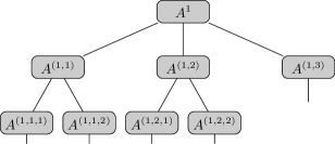
Figure 1: Representation of a tree tensor network for a five-dimensional wavefunction. Each node of the tree corresponds to a coefficient tensor, and the lines connecting nodes represent the contraction over indices common to the two nodes.

The expression of a wavefunction in a ML-MCTDH format is non-unique since the product of a matrix $M$ and its inverse $M^{-1}$ can be inserted between any two coefficient tensor sharing a common index without changing the value of the wavefunction. However, we can impose gauge conditions on the tensors to remove this ambiguity. For example, we can, as is done in ML-MCTDH, require all non-root coefficient tensors satisfy the following orthonormality condition

$$A_{I^{z_{l}}i_{0}}^{*z_{l}}A_{I^{z_{l}}j_{0}}^{z_{l}}=\delta_{i_{0}j_{0}}\ \ \forall\ z_{l}\neq 1,$$ (1)

where we have introduced the notation $I^{z_{l}}=(i_{1},\dots,i_{d^{z_{l}}})$ for the combined set of indices pointing towards the leaf nodes. We also note the use of Einstein summation convention, implying summation over repeated indices, in Eq. 1 and hereafter. This orthonormality condition translates to $A^{z_{l}}\thinspace\forall\thinspace z_{l}\neq 1$ being expansion coefficients for orthonormal SPFs in the direct product basis of orthonormal SPFs (or primitive basis functions for the leaf nodes) of the child nodes of $z_{l}$. The associated SHFs are not orthonormal, i.e. they have a non-unit overlap matrix, referred to as the mean-field density matrix. The mean-field density matrix at node $z_{l}$ can be defined in terms of contractions between the SHFs of node $z_{l}$ with their complex conjugate. This leads to a recursive definition of the $\rho^{(z_{l},k)}$, the mean-field density matrix of the $k$-th child of node $z_{l}$ (node $(z_{l},k)$), in terms of the mean-field density matrix $\rho^{z_{l}}$ and coefficient tensor $A^{z_{l}}$ of node $z_{l}$

$$\rho_{ab}^{(z_{l},k)}=A_{I^{z_{l}}_{k;a}i}^{*z_{l}}\rho_{ij}^{z_{l}}A_{I^{z_{l}}_{k;b}j}^{z_{l}},$$ (2)

where $I^{z_{l}}_{k;a}=(i_{1},\dots,i_{k-1},a,i_{k+1},\dots,i_{d^{z_{l}}})$ is a combined index obtained when the $k$th index in $I^{z_{l}}$ is replaced with the value $a$. This expression makes use of Eq. 1 for all nodes that are not on the path between the root node and $z_{l}$. For the root node $z_{l}=1$, Eq. 1 translates to $A^{1}$ being expansion coefficients for the full wavefunction in the orthonormal basis defined by the remainder of the tree, and it is not subject to any constraint besides normalization. To denote this special property, we will decorate its coefficient tensor with a tilde-symbol, namely $\widetilde{A^{1}}{\!\;\!}$.

Having obtained an unambigous ML-MCTDH representation of the wavefunction through the constraint in Eq. 1, we can treat the coefficient tensors as variational parameters and obtain a solution to the time-dependent Schrödinger equation using the time-dependent variational principle. To do this we need to further specify a dynamic gauge condition for the overlap of coefficient tensors with their time-derivative. Here, for simplicity, we will make use of the standard choice, namely that these two matrices are orthogonal for all nodes except the root node. This leads to the following EOMs for the coefficient tensor at the root node

$$\dot{\widetilde{A}}{\!\;\!}_{I^{1}}^{1} =-\frac{{i}}{\hbar}\sum_{r}h_{r;I^{1}J^{1}}^{1}\widetilde{A}{\!\;\!}_{J^{1}}^{1},$$ (3)

and at all other nodes

$$\dot{A}_{I^{z_{l}}i_{0}}^{z_{l}}\!=\!-\frac{{i}}{\hbar}\!\sum_{r}\!Q_{I^{z_{l}}\!K^{z_{l}}}^{z_{l}}h_{r;K^{z_{l}}\!J^{z_{l}}}^{z_{l}}A_{J^{z_{l}}\!j}^{z_{l}}H_{r;jk}^{z_{l}}[(\rho^{z_{l}})^{\text{-}1}]_{ki_{0}}.$$ (4)

Here, we have written the Hamiltonian in a sum-of-product (SOP) form, $\hat{H}=\sum_{r}\bigotimes_{a\in L}\hat{h}_{r}^{a}$, with $L$ denoting the set of leaf nodes and $\hat{h}_{r}^{a}$ is the Hamiltonian operator acting on the physical degree of freedom associated with leaf-node $a$. The Hamiltonian at each node can be expressed in terms of the matrices

$$h_{r;I^{z_{l}}J^{z_{l}}}^{z_{l}}= \prod_{k=1}^{d^{z_{l}}}A_{I^{(z_{l},k)}i_{k}}^{*(z_{l},k)}h_{r;I^{(z_{l},k)}J^{(z_{l},k)}}^{(z_{l},k)}A_{J^{(z_{l},k)}j_{k}}^{(z_{l},k)}$$ (5)

$$= \prod_{k=1}^{d^{z_{l}}}M_{r;i_{k}j_{k}}^{(z_{l},k)},$$

where $I^{(z_{l},k)}=(i_{1},\dots,i_{d}^{(z_{l},k)})$ is the combined index for all indices associated with all children of node $(z_{l},k)$, and

$$H_{r;ab}^{(z_{l},k)}=A_{I^{z_{l}}_{k;a}i}^{*z_{l}}\left(\prod_{\begin{subarray}{c}k^{\prime}=1\\ k^{\prime}\neq k\end{subarray}}^{d^{z_{l}}}M_{r;i_{k^{\prime}}j_{k^{\prime}}}^{(z_{l},k^{\prime})}\right)H_{r;ij}^{z_{l}}A_{I^{z_{l}}_{k;b}j}^{z_{l}}.$$ (6)

The Hamiltonians in Eqs. 5 and 6 are referred to as the SPF and mean-field Hamiltonian matrices, respectively. They can be considered as matrix elements of operators present in the SOP expansion evaluated using the SPFs and SHFs, respectively. Additionally, the projector onto the space spanned by the SPFs of node $z_{l}$ appears in Eq. 4, and is defined as

$$Q_{I^{z_{l}}J^{z_{l}}}^{z_{l}}=\delta_{I^{z_{l}}J^{z_{l}}}-A_{I^{z_{l}}i}^{z_{l}}A_{J^{z_{l}}i}^{*z_{l}}.$$ (7)

The presence of this projector makes Eq. 4 non-linear. Furthermore, Eq. 4 contains the inverse of the mean-field density matrix, $(\rho^{z_{l}})^{-1}$. Since the density matrix is not guaranteed to be of full rank and is often almost rank-deficient, Eq. 4 can be singular and requires regularization of the matrix inverse in order to be numerically solvable.

II.2 Singularity-Free Versions of ML-MCTDH

In order to circumvent the presence of an ill-defined inverse in the ML-MCTDH EOMs, we can make use of the gauge freedom in the ML-MCTDH representation of the wave function. In particular, we can choose a representation in which both SHFs and SPFs for a given node $z_{l}$ are orthonormal by imposing the following orthonormality condition

$$A_{I^{z_{l}^{\prime}}_{p(z_{l});a}i}^{*z_{l}^{\prime}}A_{I^{z_{l}^{\prime}}_{p(z_{l});b}i}^{z_{l}^{\prime}}=\delta_{ab}\ \forall\ z_{l}^{{}^{\prime}}\neq z_{l},$$ (8)

where $p(z_{l})$ indicates the index of the array which points towards node $z_{l}$, and $I^{z_{l}^{\prime}}_{p(z_{l});a}$ is a combined index of the form used previously. For all nodes that are not node $z_{l}$ or ancestors of node $z_{l}$ (namely they are not its parent or parent’s parent, and so on up to the root node), the index pointing to the $p^{z_{l}}$ node is the same as the index pointing towards the root node ($p(z_{l})=p(1)$). For these nodes Eq. 8 is equivalent to Eq.  1. For the nodes that are ancestors of node $z_{l}$, this corresponds to a different orthonormality condition. Imposing this condition alters the value of the coefficient tensors for these nodes. To make this explicit, we will choose a different label, $U^{z_{l}}$, for the coefficient tensors of nodes that satisfy Eq. 8 and are ancestors of node $z_{l}$. This orthogonality condition leads to orthonormal SPFs for all nodes which are not ancestors of node $z_{l}$, and orthonormal SHFs for node $z_{l}$ and all of its ancestors. The latter property can be straightforwardly verified by comparison with Eq. 2. Note that Eq. 1 is obtained as a special case ($z_{l}=1$) of Eq. 8.

Singularity-free approaches to propagating the ML-MCTDH wavefunction make use of this representation, in which the inverse of the density matrix $\rho^{z_{l}}$ is trivially the identity matrix. In the following, we will discuss a particular singularity-free method to propagate ML-MCTDH wavefunctions, the projector splitting integrator (PSI). This algorithm can be considered as a linearized integrator for singularity-free ML-MCTDH EOMs, similar to the commonly used constant-mean-field integrator for standard ML-MCTDH EOMs. Instead of solving Eq. 4 for the non-root node coefficient tensors under the orthonormality constraint Eq. 1, the PSI involves solving two differential equations for every node $z_{l}$ serially, that is node-by-node. First, we propagate the coefficient tensor $\widetilde{A}{\!\;\!}^{z_{l}}$ forward in time, where the tilde-symbol indicates that we enforce orthonormality condition in Eq. 8 for node $z_{l}$ according to

$$\dot{\widetilde{A}}{\!\;\!}_{I^{z_{l}}i_{0}}^{z_{l}}(t)=-\frac{{i}}{\hbar}\sum_{r}h_{r;I^{z_{l}}J^{z_{l}}}^{z_{l}}\widetilde{A}{\!\;\!}_{J^{z_{l}}j}^{z_{l}}(t)\widetilde{H}{\!\;\!}_{r_{ji_{0}}}^{z_{l}}.$$ (9)

Here, we explicitly denote time-dependence, and the other quantities are taken to be time-independent, which renders Eq. 12 linear. Tilde-symbols on the SHF Hamiltonian matrices are used to indicate that these quantities are evaluated using orthonormal SHFs. The SPF Hamiltonian matrix elements are unchanged from those in Eq. 4. Note that the structure of Eq. 9 is similar to Eq. 4, with the exception of the omission of the mean-field density matrix inverse, which is trivially the identity matrix due to the chosen orthonormality condition and the second term in projector $Q^{z_{l}}$ (see Eq. 7). Second, we use an orthogonal decomposition

$$\widetilde{A}{\!\;\!}_{I^{z_{l}}i_{0}}^{z_{l}}=A_{I^{z_{l}}j_{0}}^{z_{l}}R_{j_{0}i_{0}}^{z_{l}}\quad|\quad A_{I^{z_{l}}j_{0}}^{*z_{l}}A_{I^{z_{l}}j_{0}^{\prime}}^{z_{l}}=\delta_{j_{0},j_{0}^{\prime}},$$ (10)

which gives a different orthonormality condition,

$$U_{I^{z_{l}}_{p(z_{l});a}i}^{*z_{l}^{\prime}}U_{I^{z_{l}}_{p(z_{l})b}i}^{z_{l}^{\prime}} =\delta_{ab}\ \forall\ z_{l}^{{}^{\prime}}\in\mathrm{ancestors}(z_{l}),$$ (11)

$$A_{I^{z_{l}}i}^{*z_{l}^{\prime}}A_{I^{z_{l}}j}^{z_{l}^{\prime}} =\delta_{ij}\ \forall\ z_{l}^{\prime}\not\in\mathrm{ancestors}(z_{l}),$$

where $\mathrm{ancestors}(z_{l})$ denotes the set of nodes that are ancestors of node $z_{l}$. We can interpret $R^{z_{l}}$ as an additional, temporary node in the tree. We propagate $R^{z_{l}}$ backwards in time according to

$$\dot{R}_{ij}^{z_{l}}(t)=-\frac{{i}}{\hbar}\sum_{r}A_{K^{z_{l}}i}^{*z_{l}}h_{r;K^{z_{l}}J^{z_{l}}}^{z_{l}}A_{J^{z_{l}}k}^{z_{l}}{R}_{kl}^{z_{l}}(t)\widetilde{H}{\!\;\!}_{r;lj}^{z_{l}}.$$ (12)

The structure of Eq. 12 is again similar to that of Eq. 4, with the exception that Eq. 12 only accounts for the nontrivial term in projector $Q^{z_{l}}$ and the lack of the inverse of the density matrix due to the chosen orthonormality condition. The fact that this equation is solved backwards in time stems from the negative sign in front of the second term in projector $Q^{z_{l}}$. The requirement to solve Eqs. 9 and 12 sequentially, one node at a time, arises from the change of orthonormality conditions associated with propagating different nodes. Note that seriality is not inherently necessary for singularity-free approaches, as discussed in the companion paper and in Refs. Weike and Manthe, 2021 and Ceruti and Lubich, 2021.

The PSI involves the changing of orthonormality conditions between different nodes interspersed with the solution of linear differential equations. In the following, we will introduce how to efficiently convert between ML-MCTDH wavefunctions with different orthonormality conditions before discussing the algorithm in detail.

II.3 Conversion Between Different Orthonormality Conditions and Update of Hamiltonian Matrix Elements

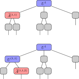
Figure 2: Diagrammatic representations of the ML-MCTDH wavefunction from Fig. 1 transformed into the alternative representation where both the SPF and SHFs of node $z_{l}$ are orthonormal. For the top tree $z_{l}=(1,1)$, while for the bottom tree $z_{l}=(1,1,2)$. The coefficient tensors of the unlabelled (grey) nodes satisfy the orthonormality condition given in Eq. 1, and are left unchanged by this transformation. The coefficient tensors of the nodes labelled with $U^{z_{l}}$ (blue) satisfy the orthonormality condition given in Eq. 8, and so will generally differ from the standard coefficient tensors. Finally, the coefficient tensors labelled with $\widetilde{A}{\!\;\!}^{z_{l}}$ (red) are the transformed coefficient tensors given by Eq. 10 that evolves according to the EOM given in Eq. 9.

The orthonormality condition used in ML-MCTDH (Eq. 1) is just the special case of the orthonormality condition given in Eq. 8 when $z_{l}=1$. In order to be able to convert between Eq. 1 and Eq. 8 for any arbitrary $z_{l}$ and back, there are two operations we need to to perform:

• Given that Eq. 8 holds for node $z_{l}$ we need to be able to convert to a representation where it holds for the child node $(z_{l},k)$ for any value of $k$.

• Given that Eq. 8 holds for the node $(z_{l},k)$ we need to able to convert to a representation where it holds for its parent node $z_{l}$.

We will begin by assuming that we have a representation in which Eq.  8 holds for node $z_{l}$, and present how to transform the ML-MCTDH wavefunction so that this condition is enforced for a child node $(z_{l},k)$. In order to do this we need to construct a new coefficient tensor $U^{z_{l}}$ for node $z_{l}$ so that the orthogonality condition in Eq. 8 is satisfied for node $(z_{l},k)$. This tensor is related to the coefficient tensors $\widetilde{A}{\!\;\!}^{z_{l}}$ by multiplication with a matrix ${R}^{(z_{l},k)}$,

$$\widetilde{A}{\!\;\!}_{I^{z_{l}}_{k;b}i}^{z_{l}}=U_{I^{z_{l}}_{k;a}i}^{z_{l}}{R}_{ba}^{(z_{l},k)}\quad|\quad U_{I^{z_{l}}_{k;a}i}^{*z_{l}}U_{I^{z_{l}}_{k;b}i}^{z_{l}}=\delta_{ab}.$$ (13)

Note that the decomposition given in Eq. 13 is not unique, which can be seen by inserting $I=U^{-1}U$ with a unitary $U$ between ${R}^{(z_{l},k)}$ and $\widetilde{U}{\!\;\!}^{z_{l}}$. There are arbitrarily many matrices that provide equally valid decompositions. For instance, one could apply a QR matrix decomposition on $\widetilde{A}{\!\;\!}^{z_{l}}$, reshaped as a matrix of size

$$\left(\displaystyle\prod_{\begin{subarray}{c}j=0\\ j\neq k\end{subarray}}^{d^{z_{l}}}n^{z_{l}}_{j}\right)\times n^{z_{l}}_{k},$$ (14)

with $n^{z_{l}}_{0}=N^{z_{l}}$, which returns a unique decomposition with ${R}^{(z_{l},k)}$ an upper triangular matrix if $\widetilde{A}{\!\;\!}^{z_{l}}$ does not have linearly dependent columns. If $\widetilde{A}{\!\;\!}^{z_{l}}$ does have linearly dependent columns, the corresponding entries in $U^{z_{l}}$ can be chosen freely as long as they constitute orthonormal columns. Contracting the matrix ${R}^{(z_{l},k)}$ with the coefficient tensor at node $(z_{l},k)$,

$$A_{I^{(z_{l},k)}j_{0}}^{(z_{l},k)}{R}_{j_{0}i_{0}}^{(z_{l},k)}=\widetilde{A}{\!\;\!}_{I^{(z_{l},k)}i_{0}}^{(z_{l},k)},$$ (15)

leaves us with an expansion of the wavefunction in terms of orthonormal SPFs and SHFs for node $(z_{l},k)$. Since we have modified the coefficient tensor of the node $z_{l}$, we need to update the mean-field Hamiltonian matrix elements for node $(z_{l},k)$,

$$\widetilde{H}{\!\;\!}_{r;ab}^{(z_{l},k)}=U_{I^{z_{l}}_{k;a}i}^{*z_{l}}\left(\prod_{\begin{subarray}{c}k^{\prime}=1\\ k^{\prime}\neq k\end{subarray}}^{d^{z_{l}}}M_{r;i_{k^{\prime}}j_{k^{\prime}}}^{(z_{l},k^{\prime})}\right)\widetilde{H}{\!\;\!}_{r;ij}^{z_{l}}U_{I^{z_{l}}_{k;b}j}^{z_{l}},$$ (16)

where $M_{r;i_{k^{\prime}}j_{k^{\prime}}}^{(z_{l},k^{\prime})}$ is defined in Eq. 5, and in order to ensure we can apply this equation for all nodes in the tree, we will define $\widetilde{H}{\!\;\!}^{1}_{r;ij}=1$ for $i=j=1$. Note that this equation is very closely related to the standard ML-MCTDH expression for the mean-field matrix $H_{r}^{(z_{l},k)}$ for a child of node $z_{l}$, Eq. 6. It is the same expression but with $A^{z_{l}}$ replaced with $U^{z_{l}}$. As such, the process for evaluating these matrices does not change significantly when compared to standard ML-MCTDH, other than that some additional optimizations become possible due to the orthonormality of these SHFs (see Sec. IV of the Supplementary Information). Note that when transferring the orthogonality condition to a child node, the SPF Hamiltonian matrices for the child node remain unchanged and do not need to be updated.

The reverse operation, converting the orthogonality condition from node $(z_{l},k)$ to its parent node $z_{l}$ proceeds as follows. First, a decomposition of the form given in Eq. 10 is obtained,

$$\widetilde{A}{\!\;\!}_{I^{(z_{l},k)}i_{0}}^{(z_{l},k)}=A_{I^{(z_{l},k)}j_{0}}^{(z_{l},k)}{R}_{j_{0}i_{0}}^{(z_{l},k)}\quad|\quad A_{I^{(z_{l},k)}j_{0}}^{(z_{l},k)*}A_{I^{(z_{l},k)}j_{0}^{\prime}}^{(z_{l},k)}=\delta_{j_{0}j_{0}^{\prime}}.$$ (17)

Then the SPF Hamiltonian matrices for node $z_{l}$ are updated according to

$$h_{r;I^{z_{l}}J^{z_{l}}}^{z_{l}}= \prod_{k=1}^{d^{z_{l}}}A_{I^{(z_{l},k)}i_{k}}^{*(z_{l},k)}h_{r;I^{(z_{l},k)}J^{(z_{l},k)}}^{(z_{l},k)}A_{J^{(z_{l},k)}j_{k}}^{(z_{l},k)},$$ (18)

which is exactly the same expression as in the standard ML-MCTDH case. Finally we contract ${R}^{(z_{l},k)}$ with $U^{z_{l}}$,

$$\widetilde{A}{\!\;\!}_{I^{z_{l}}_{k;b}i}^{z_{l}}={R}_{ba}^{(z_{l},k)}U_{I^{z_{l}}_{k;a}i}^{z_{l}}.$$ (19)

When transferring the orthogonality condition to the parent of node $z_{l}$, the SHF Hamiltonian matrices for the parent remain unchanged and do not need to be updated, while the SHF Hamiltonian matrices for node $z_{l}$ do not appear in the algorithm’s working equations and thus do not need to recomputed.

In calculations it is not necessary to form the SPF Hamiltonian matrices $h_{r}^{z_{l}}$, all required operations can be expressed in terms of the matrices $M_{r}^{(z_{l},k)}$ associated with the child nodes of node $z_{l}$. The SPF Hamiltonian matrix is the Kronecker product of each of these matrices. This representation leads to an efficient scheme for applying the SPF Hamiltonian matrix to the coefficient tensors in terms of a series of matrix-tensor contractions. Additionally, it is useful to make use of an alternative SOP form as discussed in Sec. IV of the Supplementary Information.

We can convert a ML-MCTDH wavefunction for which Eq. 8 is satisfied for node $z_{l}$ to one for which it is satisfied for node $z_{l}^{\prime}$ by performing the above operations sequentially along the path through the tree that connects nodes $z_{l}$ and $z_{l}^{\prime}$.

II.4 Integrating the Singularity-Free Equations of Motion: the Projector Splitting Integrator

The PSI propagates the coefficient tensor at node $z_{l}$, $A^{z_{l}}$, for a fixed time step $dt$ using a wavefunction expansion with orthonormal SPFs and SHFs for node $z_{l}$, while keeping the coefficient tensors at other nodes constant during the update at node $z_{l}$. Neglecting the time dependence of quantities involving other coefficient tensors is similar in spirit to the well-established constant mean-field (CMF) integration scheme for the standard ML-MCTDH EOMs, with the exception that the PSI updates the coefficients at the nodes sequentially. The order in which nodes are propagated is in principle arbitrary. Here we will discuss an efficient and easily illustrated order, namely an Euler tour traversal,(Goodrich and Tamassia, 2010) starting from the root node. For the single-layer case this traversal reduces to the previously published version for MCTDH wavefunctions.(Kloss et al., 2017) In analogy with the single-layer version, a symmetric, second-order integrator is obtained by combining a propagation step with its adjoint. Specifically, this means that a single time-step consists of two substeps: a forward and a backward walk through the tree structure, each of which propagates all coefficient tensors by $dt/2$. We restate the equations of motion to be solved for the reader’s convenience expressed using the matrix notation employed in the companion paper:

$$\dot{\widetilde{{\boldsymbol{{A}}}}}{\!\;\!}^{\boldsymbol{{z}}_{l}}(t)=-\frac{{i}}{\hbar}\sum_{r} \boldsymbol{{h}}_{r}^{\boldsymbol{{z}}_{l}}\widetilde{{\boldsymbol{{A}}}}{\!\;\!}^{\boldsymbol{{z}}_{l}}(t)\widetilde{{\boldsymbol{{H}}}}{\!\;\!}_{r}^{\boldsymbol{{z}}_{l}},$$ (20)

and

$$\dot{{\boldsymbol{{R}}}}{}^{\boldsymbol{{z}}_{l}}(t)= -\frac{{i}}{\hbar}\sum_{r}\boldsymbol{{A}}^{\boldsymbol{{z}}_{l}\dagger}\boldsymbol{{h}}_{r}^{\boldsymbol{{z}}_{l}}\boldsymbol{{A}}^{\boldsymbol{{z}}_{l}}\boldsymbol{{R}}^{\boldsymbol{{z}}_{l}}(t)\widetilde{{\boldsymbol{{H}}}}{\!\;\!}_{r}^{\boldsymbol{{z}}_{l}},$$ (21)

for $z_{l}\neq 1$, and

$$\dot{\widetilde{\boldsymbol{A}}}{\!\;\!}^{1}(t)=-\frac{i}{\hbar}\boldsymbol{{h}}{}^{1}\widetilde{\boldsymbol{A}}{\!\;\!}^{1}(t)$$ (22)

for the root node coefficient tensor. The integrator is described schematically in Fig. 3 and verbally in the following paragraphs.

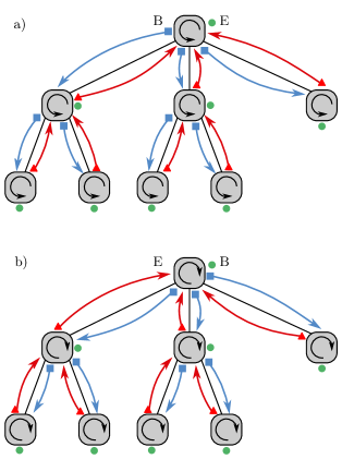
Figure 3: The two node traversal schemes used in the implementation of the PSI described in this work. a) Represents the forward walk step. b) Representation of the backwards walk step. The blue squares correspond to the construction of the orthonormal SHFs followed by the updating of mean-field matrices. The green circles correspond to evolution of the transformed coefficient tensors. The red triangles correspond to reformation of the standard coefficient tensors. The arrows connecting nodes correspond to transfers of the non-orthogonal $\boldsymbol{{R}}^{z}(t)$ matrix between nodes of the tree, and the black arrows in each node indicate the order in which these operations occur, e.g. operations on a node are applied counter-clockwise in the forward step and clockwise in the backwards step. For both walks the beginning (B) and end (E) points are shown.

Forward walk:

The forward walk starts and ends with a wavefunction that fulfills Eq. 8 for the root node $z_{l}=1$. The walk on the tree is counter-clockwise, namely the next node will always be the closest to the last visited node in a counter-clockwise direction. This ensures that every link on the tree is traversed exactly twice, once while descending and once while ascending. The first node visited after the root node is its leftmost child node. During the forward walk, descending the tree only involves transferring the orthonormality condition given by Eq. 8 from node $z_{l}$ to the next node (one of its children), according to the procedure outlined above. Furthermore, we update the mean-field Hamiltonian matrix elements, $\widetilde{{\boldsymbol{{H}}}}{\!\;\!}_{r}^{\boldsymbol{{z}}_{l}}$, to be consistent with the current expansion of the wavefunction (see Eq. 13). When the walk ascends from node $(z_{l},k)$ to node $z_{l}$, we solve the EOMs Eqs. 20 and 21. Specifically, we propagate $\widetilde{\boldsymbol{A}}{\!\;\!}^{(z_{l},k)}(t_{0})$ to $\widetilde{\boldsymbol{A}}{\!\;\!}^{(z_{l},k)}(t_{0}+dt/2)$ using Eq. 20 and for all non-root nodes use the decomposition $\widetilde{\boldsymbol{A}}{\!\;\!}^{(z_{l},k)}(t_{0}+dt/2)={\boldsymbol{{A}}}^{(z_{l},k)}(t_{0}+dt/2)\boldsymbol{R}^{(z_{l},k)}(t_{0}+dt/2)$ (see Eq. 17). After updating SPF Hamiltonian matrix elements of node $z_{l}$ using ${\boldsymbol{{A}}}^{(z_{l},k)}(t_{0}+dt/2)$ (see Eq. 18), we propagate $\boldsymbol{R}^{(z_{l},k)}(t_{0}+dt/2)$ backwards in time to $\boldsymbol{R}^{(z_{l},k)}(t_{0})$ using Eq. 21. Contracting $\boldsymbol{R}^{(z_{l},k)}(t_{0})$ with the coefficient tensor of node $z_{l}$ establishes the orthogonality condition Eq. 8 for node $z_{l}$ and completes the step from node $(z_{l},k)$ to $z_{l}$.

Backward walk:

The backward walk starts and ends with a wavefunction that fulfills Eq. 8 for $z_{l}=1$, i.e. at the root node. The walk on the tree is clockwise, i.e. the next node is the closest to the last visited node in a clockwise direction. During the walk, every link on the tree is traversed exactly twice, once while descending and once while ascending. The first node visited after the root node is its rightmost child node. During the backward walk, ascending the tree only involves transferring the orthonormality condition given by Eq. 8 from a node $(z_{l},k)$ to its parent node $z_{l}$. Furthermore, we will update the SPF Hamiltonian matrix elements, $\boldsymbol{h}_{r}^{z{l}}$, to be consistent with the current expansion of the wavefunction (see Eq. 18). When the walk descends from node $z_{l}$ to node $(z_{l},k)$, we solve the EOMs Eqs. 20 and 21. Specifically, we obtain $\boldsymbol{R}^{(z_{l},k)}$ by decomposing $\widetilde{\boldsymbol{A}}{\!\;\!}^{z_{l}}$ according to Eq. 13, update the mean-field matrix elements for node $(z_{l},k)$ (see Eq. 16) and propagate $\boldsymbol{R}^{(z_{l},k)}$ backwards in time from $\boldsymbol{R}^{(z_{l},k)}(t_{0}+dt)$ to $\boldsymbol{R}^{(z_{l},k)}(t+dt/2)$ using Eq. 21. $\boldsymbol{R}^{(z_{l},k)}(t+dt/2)$ is contracted with ${\boldsymbol{{A}}}^{(z_{l},k)}(t_{0}+dt/2$) (see Eq. 15), yielding $\widetilde{\boldsymbol{A}}{\!\;\!}^{(z_{l},k)}(t_{0}+dt/2)$ and restoring the orthogonality condition Eq. 8 for node $(z_{l},k)$. $\widetilde{\boldsymbol{A}}{\!\;\!}^{(z_{l},k)}(t_{0}+dt/2)$ is propagated forward in time according to Eq. 20, which completes the step from node $z_{l}$ to $(z_{l},k)$.

II.5 Discussion of the PSI

The PSI can be readily implemented within existing ML-MCTDH implementations. Since the working equations are similar to those employed in standard ML-MCTDH, the only components which may not already be part of the code are the Euler tour traversal and the orthonormal decomposition of coefficient tensors in Eq. 13. Algorithms for the former are readily available,(Goodrich and Tamassia, 2010) and efficient linear algebra routines to perform an orthogonal matrix decompositionare part of most linear algebra packages. Employing the latter requires reshaping of the coefficient tensor into a matrix with size given by Eq. 14, with $k$ chosen as required.

A potential drawback of the PSI presented here is its inherent seriality. CMF schemes for ML-MCTDH on the other hand allow for straightforward parallel integration. Parallel versions of the PSI should be possible to construct, with a version for single-layer MCTDH having already been proposed (Ceruti and Lubich, 2021) and a related scheme having been discussed for ML-MCTDH.(Weike and Manthe, 2021) At present, such approaches tend to require much smaller time steps than the PSI (see Sec. II of the Supplementary Information), which largely negates the speedup obtained through parallelization in many cases.

The PSI has been shown to be stable with respect to almost or fully rank deficient wavefunction parametrizations in its MCTDH(Kloss et al., 2017) and ML-MCTDH formulations,(Bauernfeind and Aichhorn, 2020; Kloss et al., 2020; Ceruti et al., 2021a; Lindoy, 2019) including the important subcategory of matrix product states (maximally layered trees with physical degrees of freedom at each layer).(Schröder and Chin, 2016; Kloss et al., 2018; Paeckel et al., 2019) The stability of the PSI with respect to nearly rank-deficient wavefunction parametrizations can be attributed to the fact that the EOMs solved are always well-conditioned. In ML-MCTDH, the regularization parameter controls how ill-conditioned the equations are and how rapidly the variational parameters with vanishing weight in the wavefunction expansion evolve. In addition, it influences the weight above which the evolution of these parameters becomes accurate. The PSI on the other hand has no adjustable parameter except for time-step size, and rank-deficiency leads to non-uniqueness of the orthogonal decomposition but does not increase the stiffness of the underlying EOMs. In exceptional cases, any ML-MCTDH approach can suffer from inaccurate results for certain choices of initial unoccupied SPFs(Manthe, 2018) and the PSI could additionally show dependence on the choice of redundant parameters in the orthogonal decompositions. We will provide numerical evidence in the following that this effect can be suppressed by simply increasing the number of SPFs.

The following section will address the lack of benchmarks and demonstrate the stability and performance of the PSI in a set of typical applications of ML-MCTDH. Before we move on, we would like to point to developments towards a dynamical adaption of the number of SPFs at each node of the ML-MCTDH expansion during the propagation.(Larsson and Tannor, 2017; Yang and White, 2020; Mendive-Tapia and Meyer, 2020; Ceruti et al., 2021b) These approaches can speed up challenging calculations, but more importantly algorithms that make use of higher powers of the Hamiltonian(Yang and White, 2020; Mendive-Tapia and Meyer, 2020) address, at least partially, the fundamental shortcoming of the time-dependent variational principle. They provide information about the optimal evolution of redundant variational parameters, however at the cost of requiring the evaluation of the action of higher powers of the Hamiltonian on the wavefunction. While some of these approaches have been formulated for matrix product states, they are equally applicable to generic ML-MCTDH wavefunctions.

III Results

In order to demonstrate the capabilities of the PSI, we will consider a series of 3 models. The first, a simple two-dimensional bi-linearly and bi-quadratically coupled harmonic oscillator model, will be used to explore the extent to which the choice of unoccupied SPFs influences the dynamics obtained. The second set of models will be a series of spin-boson models with strong system-bath coupling and varying numbers of bath modes. This set of models will be used to demonstrate the effect that increasing the bath size has on the convergence properties of the PSI and how well the PSI can treat Hamiltonians with terms that couple all modes to all other modes. The final set of models that will be considered are a series of multi-spin-boson models with varying numbers of two-level systems (TLSs). These models will serve as a test of the PSI when larger number of SPFs are required at each node.

III.1 Two-Dimensional, Bi-Linearly and Bi-Quadratically Coupled Harmonic Oscillator Model

We start by considering a two-dimensional oscillator model that is described by the Hamiltonian(Manthe, 2015a)

$$\hat{{H}}= \frac{{1}}{2}\left(-\frac{{\partial^{2}}}{\partial x^{2}}+x^{2}\right)+\frac{{1}}{2}\left(-\frac{{\partial^{2}}}{\partial y^{2}}+x^{2}\right)$$ (23)

$$+\frac{{1}}{4}xy+\frac{{1}}{2}\left(x^{2}-\frac{{1}}{2}\right)\left(y^{2}-\frac{{1}}{2}\right).$$

This model is particularly useful when assessing the behavior of unoccupied SPFs. When the initial wavefunction is taken to be the non-interacting ground state, ($\Psi_{0}(x,y)=\chi_{0}(x)\chi_{0}(y)$, where $\chi_{n}$ is the n-th eigenfunction of the unitless one-dimensional harmonic oscillator), it is possible to evaluate the optimal unoccupied SPFs analytically, and their short time evolution, giving(Manthe, 2015a)

$$\phi_{opt}^{(1)} (z)=\chi_{2}(z),$$ (24)

$$\phi_{opt}^{(2)} (z)=\chi_{1}(z),\ \ \ z=x,y.$$ (25)

For short times, the first of these function will provide the dominant correction to the evolution of the wavefunction and will be referred to as the dominant unoccupied SPF. In Ref. Manthe, 2015a, it was demonstrated that when two SPFs are used for each mode, the dynamics obtained by conventional MCTDH are sensitive to the choice of the initially unoccupied SPF. The dynamics obtained using the PSI has also been shown to exhibit a dependence on the initially unoccupied SPFs.(Kloss et al., 2017) When the unoccupied SPF initially has considerable overlap with the non-dominant unoccupied SPF, Eq. 25, it may not capture the dominant contribution to the dynamics. It should be noted that in these tests, only a very specific set of initial conditions are considered.

Here we consider a series of different initial configurations in an attempt to further explore the dependence on initial conditions. We will employ a $N_{hilb}$-dimensional Hilbert space of harmonic oscillator basis functions for each mode and uniformly sample normalized unoccupied SPFs within the space that is orthogonal to the harmonic oscillator ground state. In Table 1, we present the percentage of wavepacket evolutions (out of a total of 1000) in which the unoccupied SPF did not evolve following the dominant unoccupied SPFs.

$N_{SPF}$	$2$
$N_{hilb}$	$10$	$10^{2}$	$10^{3}$	$10^{4}$
$\%_{f}$	0	0	1.2	10.8
$N_{SPF}$	$3$
$N_{hilb}$	$10$	$10^{2}$	$10^{3}$	$10^{4}$
$\%_{f}$	0	0	0	0

Table 1: The percentage of wavepacket evolutions ($\%_{f}$) where the unoccupied SPFs failed to evolve following the dominant unoccupied SPF for different local Hilbert space dimensions ($N_{hilb}$). 1000 wavepacket evolutions were performed for each case with the initial states of the unoccupied SPFs being uniformly sampled from the space orthogonal to the harmonic oscillator ground state. Here we consider cases where we have 2 and 3 SPFs per mode.

When using two SPFs per mode we observe that none of the 1000 trajectories that were run fail to evolve according to the dominant optimal unoccupied SPF when using primitive Hilbert space dimension of up to 100. It is only for large primitive Hilbert space dimensions (10000), that an appreciable number of trajectories ($\sim 11\%)$ follow the non-dominant solution. The average overlap of a randomly sampled vector in a $D$-dimensional space with an arbitrary vector in this space scales as $D^{\text{\text{{-}}}1}$. As such, for small local Hilbert space dimensions a randomly sampled vector will, on average, have a relatively large overlap with the dominant solution, and at least for this model will track the dominant solution.

As has previously been observed for the PSI,(Kloss et al., 2017) when 3 SPFs are used per mode the dynamics becomes independent of the states of the initially unoccupied SPFs, and all trajectories track the two optimal unoccupied SPFs. This suggests that, at least for this model, the issues associated with the unoccupied SPFs are a result of insufficient convergence with respect to the number of SPFs. While one of the unoccupied SPF provides the larger contribution to the dynamics initially, both contribute considerably to the dynamics, and as soon as there are enough SPFs to capture both important SPFs, the dependence on initial conditions entirely vanishes. As the number of SPFs increases towards a full Hilbert space calculation, the PSI is guaranteed to produce the correct result regardless of the initially unoccupied SPFs. Additionally, even when there are insufficiently many SPFs, this problem is unlikely to manifest unless specific poor choices of the initially unoccupied SPF are selected. Whether this holds true generally is outside of the scope of this work. However we do not observe issues related to the initially unoccupied SPFs in the following applications to models that are more representative of those that would be treated using ML-MCTDH based approaches.

III.2 Spin-Boson Model

The two-mode model treated in the previous section is not particularly representative of the types of models conventionally treated using ML-MCTDH. We now consider a number of larger problems, starting with a series of spin-boson models in which a single two-level system (TLS) is linearly coupled to a harmonic bath.(Garg et al., 1985; Leggett et al., 1987; Nitzan, 2006; Weiss, 2012) The spin-boson Hamiltonian may be written as

$$\hat{{H}}=\varepsilon\hat{{\sigma}}_{z}+\Delta\hat{{\sigma}}_{x}+\hat{{\sigma}}_{z}\sum_{k}g_{k}(\hat{{a}}_{k}^{\dagger}+\hat{{a}}_{k})+\sum_{k}\omega_{k}\hat{{a}}_{k}^{\dagger}\hat{{a}},$$ (26)

where $\hat{{a}}_{k}^{\dagger}$ and $\hat{{a}_{k}}$ are the bosonic creation and annihilation operators associated with the $k$th bath mode, and

$$\hat{{\sigma}}_{x}=\left|0\right\rangle\left\langle 1\right|+\left|1\right\rangle\left\langle 0\right|$$ (27)

and

$$\hat{{\sigma}}_{z}=\left|0\right\rangle\left\langle 0\right|-\left|1\right\rangle\left\langle 1\right|$$ (28)

are Pauli matrices. The influence of the system on the bath is fully characterised by the bath spectral density(Leggett et al., 1987; Weiss, 2012)

$$J(\omega) =\frac{{\pi}}{2}\sum_{k}g_{k}^{2}\delta(\omega-\omega_{k})$$ (29)

from which the system-bath coupling constants, $g_{k}$, and bath frequencies, $\omega_{k}$, can be obtained. We will consider an Ohmic spectral density with an exponential cutoff

$$J(\omega)=\frac{{\pi}}{2}\alpha\omega e^{-\omega/\omega_{c}},$$ (30)

where $\alpha$ is the dimensionless Kondo parameter and $\omega_{c}$ is the cutoff frequency of the bath.

An alternative representation of the spin-boson Hamiltonian can be obtained by applying the polaron transform (Weiss, 2012)

$$\hat{{T}}=\exp\left[-\hat{{\sigma}}_{z}\sum_{k}\frac{{g_{k}}}{\omega_{k}}\left(\hat{{a}}_{k}^{\dagger}-\hat{{a}}_{k}\right)\right],$$ (31)

which displaces the bath modes depending on the states of the TLS, to this Hamiltonian. The polaron-transformed spin-boson Hamiltonian can be written as

$$\hat{{H}}_{pol}= \hat{{T}}^{\dagger}\hat{{H}}\hat{{T}}$$ (32)

$$= \varepsilon\hat{{\sigma}}_{z}+\sum_{k}\omega_{k}\hat{{a}}_{k}^{\dagger}\hat{{a}}$$

$$+ \left[\hat{{\sigma}}_{+}\exp\left[-2\sum_{k}\frac{{g_{k}}}{\omega_{k}}\left(\hat{{a}}_{k}^{\dagger}-\hat{{a}}_{k}\right)\right]+\mathrm{{h.c.}}\right],$$

in which the final term directly couples all bath and system modes in a multiplicative fashion. It has previously been show that the polaron-transformed spin-boson model provides a considerably harder challenge for ML-MCTDH than the standard representation.(Meyer and Wang, 2018; Wang and Meyer, 2018)

Before we can apply the PSI to simulating the unitary dynamics arising from either of these Hamiltonians, it is necessary to discretize the bath and consequently the spectral density. Following standard approaches,(Wang et al., 2001; Wang and Meyer, 2018) we will consider a discrete bath of $N$ modes with system-bath coupling constant given by

$$g_{k}^{2}=\frac{{2}}{\pi}\frac{{J(\omega_{k})}}{\rho(\omega_{k})}.$$ (33)

Here, $\rho(\omega)$ is the density of frequencies, which is taken to be

$$\rho(\omega)=\gamma e^{-\omega/\omega_{c}},$$ (34)

with $\gamma$ chosen to ensure correct normalization and the frequencies are given by

$$\begin{split}\int_{0}^{\omega_{k}}\rho(\omega)\mathrm{{d}\omega}=k,&\ \ \ \ k=1,2,3,\dots,N.\end{split}$$ (35)

In the following discussion, we will consider the time-dependent population difference between the states of the two-level system as our observable of interest. This population difference is given by

$$P(t)=\left\langle\Psi(t)\right|\hat{{\sigma}}_{z}\left|\Psi(t)\right\rangle,$$ (36)

where the initial wavefunction is taken as

$$\left|\Psi(0)\right\rangle=\left|0\right\rangle\otimes\left|vac\right\rangle,$$ (37)

with $\left|vac\right\rangle$ denoting the vacuum state of the bath in the standard representation. Note here we only work at $T=0$. Following Refs. Wang and Meyer, 2018 and Wang and Meyer, 2021, we will quantify the convergence of the population dynamics by using the relative cumulative deviation

$$\Delta P=\frac{{1}}{\left(P_{max}-P_{min}\right)}\frac{{1}}{\tau}\int_{0}^{\tau}|P(t)-P_{ref}(t)|\mathrm{{d}}t$$ (38)

from the population difference obtained from some reference calculation, $P_{ref}(t)$, obtained over a time period $\tau$. Here, $P_{min}$ and $P_{max}$ are the minimum and maximum population differences throughout this time-period.

We will consider a relatively strongly coupled, unbiased ($\epsilon=0$) spin-boson model with $\alpha=2$ and a cutoff frequency of $\omega_{c}=25\Delta$. For all calculations here and in the Supplementary Information, the tree structure is constructed as follows. On the top layer, we consider $N_{b}+1$ groups of SPFs, 1 of which accounts for the system degrees of freedom and contains a complete basis for the system (here this is 2 functions). The remaining $N_{b}$ groups of SPFs treat the bath degrees of freedom, with the bath modes being partitioned between the groups so that they contain modes of similar frequencies. The bath SPFs in each of the $N_{b}$ groups are then represented using as close to a balanced tree as possible with each node having up to $N_{lower}$ SPF groups. Mode combination and adiabatic contraction are used for the bottom layer, with modes being grouped up to some maximum local Hilbert space.

Standard Representation

We will begin by considering a bath of $N=500$ oscillators with $N_{b}=2$ and $N_{lower}=2$, and we will use 16 SPFs at each node in the bath subtrees. For each bath mode we will use a basis of 15 harmonic oscillator eigenfunctions and will allow for a maximum combined Hilbert space dimension of 3000. This will typically allow for 3 bath modes to be combined. We use an adaptive order, adaptive time step Lanczos integration scheme(Park and Light, 1986; Sidje, 1998) for integrating the linear systems of equations associated with each node, and in all calculations that follow we used an integration tolerance of $10^{\text{{-}12}}$. In Table III of the Supplementary Information we consider the effect of varying this tolerance on the accuracy and efficiency of the simulations, and find that such a tolerance is more than sufficient to provide converged dynamics.

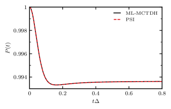
Figure 4: The time-dependent expectation value $P(t)$ obtained for a spin-boson model with $\varepsilon/\Delta=0$, $\alpha=2$, $\omega_{c}=25\Delta$, and with $N=500$ bath modes. Here the results obtained using the PSI are compared against the results obtained using the standard ML-MCTDH approach in Ref. Wang and Meyer, 2018.

The dynamics of $P(t)$ for this model has previously been obtained using standard ML-MCTDH and with the alternative regularization scheme mentioned in the introduction.(Wang and Meyer, 2018) In Fig. 4, we compare the results obtained using the PSI to their results in an effort to demonstrate the validity of our implementation of the PSI. Here we see population difference dynamics that agree well over the entire time period considered. Having validated our implementation of the multi-layer version of the PSI, we are now in a position to look at some more challenging cases.

Polaron-Transformed Representation

It has previously been shown that the standard ML-MCTDH approach fails to capture the dynamics of the polaron-transformed representation of the spin-boson model.(Meyer and Wang, 2018; Wang and Meyer, 2018) This is due to the inability of the regularized ML-MCTDH EOMs to accurately capture the rapid evolution of unoccupied SPFs required for this representation, and an alternative regularization scheme is required to obtain accurate dynamics.(Meyer and Wang, 2018; Wang and Meyer, 2018) In panel a) of Fig. 5, we present the dynamics of the polaron-transformed representation of the spin-boson model considered in Fig. 4 obtained using the PSI with a range of constant time steps.

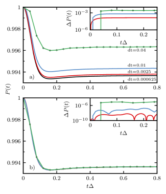
Figure 5: The effect of time step on the convergence of $P(t)$ for a polaron-transformed spin-boson model with $\varepsilon/\Delta=0$, $\alpha=2$, $\omega_{c}=25\Delta$, and with $N=500$ bath modes. a) Results obtained using a fixed time step integrator (with time steps shown). b) Results alternative scheme that makes use of a series of smaller time steps to integrate form $t=0$ to $t=dt$ but uses the same fixed step as in panel a) for all times $t>dt$. The insets in each panel show the absolute difference of the results obtained with a given time step and the reference calculation obtained with $dt\Delta=0.000625$.

The population dynamics obtained for the polaron-transformed Hamiltonian converges considerably slower than the population dynamics obtained when using the standard representation (shown in Fig. 4). By considering the time-dependent deviation from the reference calculation shown in the inset of panel a) of Fig. 5, it can be seen that the significant deviation observed is dominated by errors made in the first time step, following which the deviation from the reference calculations reaches a plateau. In order to accurately describe the dynamics of this Hamiltonian, and in particular the contribution arising from the final term in Eq. 32 that couples all modes to all other modes in a multiplicative manner, the SPFs need to undergo rapid evolution. Within the PSI, the coefficients for each node are evolved over each time period with the SPFs held constant. When the SPFs evolve rapidly, this provides a poor approximation to the true dynamics, as the full evolution operator quickly leaves the region of the Hilbert space described by the constant SPF and SHF basis. As such, in contrast to the standard ML-MCTDH approach where numerical issues arise from difficulties in describing this rapid evolution of SPFs, the deviations observed for the PSI can be attributed to errors associated with the constant mean-field approximation.

In order to demonstrate this point, we consider an alternative integration scheme in which the initial evolution through the interval $dt$ is split into a series of smaller time steps, with each time step being an order of magnitude larger than the previous until we reach time $t=dt$ (i.e. if 5 steps are used the first uses a time step of $10^{\text{-}5}dt$). The results obtained using this scheme are shown in panel b) of Fig. 5. With this modification to the integration protocol, we see a three orders of magnitude reduction in the deviation of the population dynamics even for a time step of $dt\Delta=0.04$, and as a consequence the population dynamics converges more rapidly in this case than for the standard spin-boson model.

These results suggest that the PSI is readily able to accurately capture rapid evolution of the initially unoccupied SPFs. In addition, this approach can benefit from an adaptive time step integration scheme. The error associated with the PSI can vary significantly throughout a simulation depending on how rapidly the SPF and mean-field Hamiltonian matrices evolve. In principle, an adaptive time step integration scheme would resolve this issue.

We have applied the adaptive integration approach described in Ref. Kloss et al., 2017 for the MCTDH case to the multi-layer case. This scheme involves propagating two approximations to the ML-MCTDH wavefunction obtained using time steps that differ by a factor of two, and as such allows for an estimate of the error of the integration to be obtained. However, we find that due to a build-up of floating point errors in the evaluation of the Hilbert angle (or overlap) between the two approximations of the wavefunction used in this approach, the error estimate itself has limited accuracy for deep tree structures ($\sim\!10^{\text{{-}6}}$). This approach provides a reasonable adaptive integration scheme when moderate integration errors are allowed ($\sim\!10^{\text{{-}5}}$), however, for problems requiring stricter tolerances we find that such an approach often becomes impractical as it is unable to accurately estimate the error.

Dependence on Initially Unoccupied SPFs

We next consider the dependence of the dynamics obtained for the model with different choices for the initially unoccupied SPFs. To do this we perform a series of simulations with different initially unoccupied SPFs. For each node in the tree, we sample the coefficients of the unoccupied SPF uniformly within the local Hilbert space such that they are orthogonal to our initially occupied state. We run a series of 20 different simulations for both the standard and polaron-transformed spin-boson model with $N=500$ bath modes, and consider the average relative cumulative deviation over the 20 trajectories taking the mean of all trajectories as the reference. The resultant mean deviations are given in Table 2.

$dt\Delta$	$\left\langle\Delta P\right\rangle$ : Standard	$\left\langle\Delta P\right\rangle$ : Polaron
$4\times 10^{\text{-2}}$	$1.9\times 10^{\text{-3}}$	$3.0\times 10^{\text{-4}}$
$2\times 10^{\text{-2}}$	$9.7\times 10^{\text{-5}}$	$4.7\times 10^{\text{-5}}$
$1\times 10^{\text{-2}}$	$1.0\times 10^{\text{-5}}$	$4.9\times 10^{\text{-6}}$
$5\times 10^{\text{-3}}$	$3.8\times 10^{\text{-6}}$	$1.2\times 10^{\text{-6}}$
$2.5\times 10^{\text{-3}}$	$1.5\times 10^{\text{-6}}$	$1.6\times 10^{\text{-6}}$
$1.25\times 10^{\text{-3}}$	$2.5\times 10^{\text{-7}}$	$1.3\times 10^{\text{-6}}$
$6.25\times 10^{\text{-4}}$	$8.5\times 10^{\text{-8}}$	$1.7\times 10^{\text{-6}}$

Table 2: Average cumulative deviation of 20 simulations from their mean obtained with different initially unoccupied SPFs.

Some deviations in the population dynamics obtained with different initially unoccupied SPFs are observed. For larger time steps, these relative deviations can be rather large, on the order of $10^{\text{{-}3}}$. As the time step is decreased, the mean deviations likewise decrease, and converge towards the results shown in Fig. 4. For this problem, the choice of the redundant initial conditions does not significantly impacts the dynamics obtained provided they are converged with respect to the integration time step.

Larger Bath Sizes

Finally, for this model, we explore the effect that increasing the number of bath modes has on the accuracy and efficiency of the dynamics obtained using the PSI. We consider a series of six bath sizes ranging from 500 to $10^{6}$ modes and treat the dynamics using the standard representation for the Hamiltonian. We once again use the relative deviation with respect to a reference calculation for each bath size as a measure of the accuracy, and use the total number of Hamiltonian evaluations, $N_{MF}$, and average number of Hamiltonian applications per node, $\langle N_{H}\rangle$, as measures of efficiency. For variable mean-field based approaches, such as those considered in Refs. Wang and Meyer, 2018 and Wang and Meyer, 2021, these two quantities are the same where as for the PSI they can differ. Depending on the specific application, either of these two steps can dominate the numerical cost associated with the calculation. For all calculations we used the alternative integration scheme introduced in the previous section, and the approach outlined above for constructing the tree topology. For all trees we use 16 SPFs per node for the first nine layers of nodes (or as many layers as the tree has), and four SPFs per node for all other nodes. This corresponds to a similar tree structure to that used for this model in Ref. Wang and Meyer, 2021, and is sufficient to converge the dynamics with respect to the number of SPFs.

$N$		500		2,000		5,000
$dt\Delta$	$N_{MF}$	$\Delta P$	$\langle N_{H}\rangle$	$\Delta P$	$\langle N_{H}\rangle$	$\Delta P$	$\langle N_{H}\rangle$
$4\times 10^{\text{-2}}$	50	$1.6\times 10^{\text{-}2}$	$9.9\times 10^{2}$	$9.4\times 10^{\text{-}3}$	$8.6\times 10^{2}$	$1.3\times 10^{\text{-}2}$	$8.0\times 10^{2}$
$2\times 10^{\text{-2}}$	90	$1.6\times 10^{\text{-}4}$	$1.4\times 10^{3}$	$1.3\times 10^{\text{-}4}$	$1.3\times 10^{3}$	$2.2\times 10^{\text{-}4}$	$1.1\times 10^{3}$
$1\times 10^{\text{-2}}$	170	$1.2\times 10^{\text{-5}}$	$2.1\times 10^{3}$	$2.3\times 10^{\text{-5}}$	$1.9\times 10^{3}$	$1.6\times 10^{\text{-5}}$	$1.7\times 10^{3}$
$5\times 10^{\text{-3}}$	330	$5.0\times 10^{\text{-6}}$	$3.2\times 10^{3}$	$2.3\times 10^{\text{-6}}$	$2.9\times 10^{3}$	$3.2\times 10^{\text{-6}}$	$2.7\times 10^{3}$
$2.5\times 10^{\text{-3}}$	650	$3.4\times 10^{\text{-6}}$	$5.3\times 10^{3}$	$8.1\times 10^{\text{-7}}$	$4.9\times 10^{3}$	$7.1\times 10^{\text{-7}}$	$4.6\times 10^{3}$
$1.25\times 10^{\text{-3}}$	1290	$1.8\times 10^{\text{-7}}$	$9.3\times 10^{3}$	$2.5\times 10^{\text{-7}}$	$8.8\times 10^{3}$	$2.1\times 10^{\text{-7}}$	$8.3\times 10^{3}$
$6.25\times 10^{\text{-4}}$	2570	Reference	$1.7\times 10^{4}$	Reference	$1.6\times 10^{4}$	Reference	$1.5\times 10^{4}$
$N$		$10^{4}$		$10^{5}$		$10^{6}$
$dt\Delta$	$N_{MF}$	$\Delta P$	$\langle N_{H}\rangle$	$\Delta P$	$\langle N_{H}\rangle$	$\Delta P$	$\langle N_{H}\rangle$
$4\times 10^{\text{-2}}$	50	$1.6\times 10^{\text{-}2}$	$7.5\times 10^{2}$	$1.2\times 10^{\text{-}2}$	$6.7\times 10^{2}$	$1.4\times 10^{\text{-}2}$	$5.3\times 10^{2}$
$2\times 10^{\text{-2}}$	90	$5.1\times 10^{\text{-}4}$	$1.0\times 10^{3}$	$4.1\times 10^{\text{-}4}$	$9.5\times 10^{2}$	$3.0\times 10^{\text{-}4}$	$8.0\times 10^{2}$
$1\times 10^{\text{-2}}$	170	$1.5\times 10^{\text{-5}}$	$1.6\times 10^{3}$	$1.6\times 10^{\text{-5}}$	$1.4\times 10^{3}$	$1.7\times 10^{\text{-5}}$	$1.3\times 10^{3}$
$5\times 10^{\text{-3}}$	330	$2.6\times 10^{\text{-6}}$	$2.5\times 10^{3}$	$2.3\times 10^{\text{-6}}$	$2.4\times 10^{3}$	$4.2\times 10^{\text{-6}}$	$2.2\times 10^{3}$
$2.5\times 10^{\text{-3}}$	650	$3.9\times 10^{\text{-7}}$	$4.4\times 10^{3}$	$5.8\times 10^{\text{-7}}$	$4.1\times 10^{3}$	$1.3\times 10^{\text{-6}}$	$4.0\times 10^{3}$
$1.25\times 10^{\text{-3}}$	1290	$1.0\times 10^{\text{-7}}$	$8.1\times 10^{3}$	$2.7\times 10^{\text{-7}}$	$7.7\times 10^{3}$	$8.6\times 10^{\text{-7}}$	$7.4\times 10^{3}$
$6.25\times 10^{\text{-4}}$	2570	Reference	$1.5\times 10^{4}$	Reference	$1.4\times 10^{4}$	Reference	$1.3\times 10^{4}$

Table 3: The convergence with respect to time step ($dt$) of the deviation in the population dynamics of a spin-boson model obtained using the PSI. The spin-boson model considered has $\varepsilon/\Delta=0$, $\alpha=2$, $\omega_{c}=25\Delta$, and with varying numbers of bath modes (specified in the tables). In all cases, the dynamics was obtained using the alternative integration scheme described above and the relative cumulative deviation (from the indicated reference) was evaluated for dynamics obtained to times $t\Delta=0.8$.

In Table 3, the convergence behavior of the PSI is compared for baths with 500, 2,000, 5,000, $10^{4}$, $10^{5}$, and $10^{6}$ modes. For all bath sizes, convergence of the population dynamics (here taken to be a deviation of $\sim\!10^{\text{{-}4}}$) is observed for time steps of $dt\Delta=1\times 10^{\text{-2}}$ or smaller. As the number of bath modes increases, the average number of Hamiltonian applications required decreases slightly. However, this decrease is not particularly significant and can likely be attributed to the tree structure used. For problems with large numbers of bath modes we have a considerably larger proportion of nodes that use four SPFs rather than sixteen SPFs. For these nodes the solution of Eq. 9 using a Krylov subspace integration scheme requires slightly fewer function applications although this difference decreases as the time step decreases. For all bath sizes this corresponds to a total of 170 Hamiltonian evaluations and with $\lesssim 2\times 10^{3}$ average Hamiltonian applications per node. In comparison, standard ML-MCTDH calculations require roughly three to four orders of magnitude more mean-field evaluations and two to three orders of magnitude more Hamiltonian evaluations to obtain the same error for baths of up to $10^{4}$ modes.(Wang and Meyer, 2018, 2021) The difference in efficiency is less extreme when compared to the improved regularization scheme presented in Ref. Wang and Meyer, 2018, however even in this case the PSI requires roughly 30-80 times fewer Hamiltonian evaluation and 3-8 times fewer Hamiltonian applications for baths of up to $10^{4}$ modes. This difference becomes more pronounced when considering the $10^{5}$ mode case. For the PSI, the number of Hamiltonian evaluations and applications required for convergence is essentially independent of the number of bath modes. For the improved regularization scheme results presented in Ref. Wang and Meyer, 2021, a factor of 10 increase in the number of evaluations required is observed when moving from $10^{4}$ to $10^{5}$ modes. For reference, the PSI calculations for the $10^{5}$ mode model using a time step of $dt\Delta=1\times 10^{\text{-2}}$ required less than three hours on a single core of an Intel i5-8250U CPU.

These results suggests that for the PSI the number of Hamiltonian evaluations and applications at a given time step is limited by the physics of the problem, and as the number of bath modes increases, little change in the number of these operations occurs. For ML-MCTDH approaches that employ regularized EOMs, the required regularization parameter depends on the number of bath modes and as a consequence considerably more integration steps are required to obtain converged results for larger baths.

All calculations presented in this section have used a relatively deep tree structure. In contrast, the results obtained in Refs. Wang and Meyer, 2018 and Wang and Meyer, 2021 for this model with bath sizes up to $N=10^{4}$ were obtained using wider trees. In Table V of the Supplementary Information, we present results obtained using wider tree structures generated with $N_{b}=4$ or $5$, and $N_{lower}=4$. We find that the conclusions reached in this section do not change when using this alternative tree topology, and thus the accuracy and efficiency when measured in terms of the number Hamiltonian applications and Hamiltonian evaluations of the PSI does not depend significantly on the tree structure. In addition to these results, we have considered the full set of spin-boson models considered in Ref. Wang and Meyer, 2018. For completeness these results are presented in Sec. VII of the Supplementary Information, and once again the PSI can obtain converged results with roughly 1-2 orders of magnitude fewer Hamiltonian evaluations and comparable to an order of magnitude fewer Hamiltonian applications than the improved regularization approach.

For all of the calculations presented so far, relatively few SPFs are required to obtain converged results, and as such do not represent particularly challenging problems. We will now consider a significantly more challenging physical system for which considerably more SPFs are required in order to obtain accurate dynamics.

III.3 Multi-Spin-Boson Model

As a final application of the PSI approach we consider a generalization of the spin-boson model, in which a set of $M$ TLSs are each linearly coupled to a common harmonic oscillator bath. The Hamiltonian for this system may be written as

$$\hat{{H}}= \sum_{i=1}^{M}\left(\varepsilon\hat{{\sigma}}_{i,z}+\Delta\hat{{\sigma}}_{i,x}\right)+\sum_{k}\omega_{k}\hat{{a}}_{k}^{\dagger}\hat{{a}}$$ (39)

$$+\sum_{i=1}^{M}\hat{{\sigma}}_{i,z}\sum_{k}g_{ik}(\hat{{a}}_{k}^{\dagger}+\hat{{a}}_{k}),$$

where $\hat{{a}}_{k}^{\dagger}$ and $\hat{{a}_{k}}$ are the bosonic creation and annihilation operators associated with the $k$th bath mode, and $\hat{{\sigma}}_{i,x}$ and $\hat{{\sigma}}_{i,z}$ are the Pauli matrices associated with spin $i$. Eq. 39 provides an interesting model in which to explore the interplay between coherent system interactions and the effects of dissipation arising from the bath.(Orth et al., 2010; McCutcheon et al., 2010; Winter and Rieger, 2014; Filippis et al., 2021) For Ohmic and sub-Ohmic baths, the presence of the additional TLSs have been shown to enhance localization, reducing the system-bath coupling strength at which the delocalization to localization transition occurs.(Orth et al., 2010; McCutcheon et al., 2010; Winter and Rieger, 2014; Filippis et al., 2021) Additionally, the model with a super-Ohmic bath arises in the description of low temperature glasses,(Joffrin and Levelut, 1975; Kassner and Silbey, 1989; Brown and Silbey, 1998; Artiaco et al., 2021) where it has been suggested that signatures of many-body localization may be experimentally observable.(Artiaco et al., 2021) In what follows, we will restrict ourselves to the case of an Ohmic bath. In contrast to the standard spin-boson model, where the influence of the bath on the system is entirely encoded within the spectral density, the MSB model involves an $M\times M$ matrix of spectral densities. The elements of this matrix of spectral densities, are given by

$$J_{ij}(\omega)=\frac{{\pi}}{2}\sum_{k}g_{ik}g_{jk}\delta(\omega-\omega_{k})$$ (40)

and can be used to specify the system-bath coupling constants, $g_{ik}$, between spin $i$ and mode $k$, and the frequency of mode $k$, $\omega_{k}$. We will consider diagonal spectral densities that are Ohmic with an exponential cutoff

$$J_{ii}(\omega)=\frac{{\pi}}{2}\alpha\omega e^{-\omega/\omega_{c}},$$ (41)

and off-diagonal spectral densities of the form(Winter and Rieger, 2014)

$$J_{ij}(\omega)=\frac{{\pi}}{2}\alpha\omega e^{-\omega/\omega_{c}}\cos\left(\omega r_{ij}/\nu\right),$$ (42)

where $\alpha$ is the dimensionless Kondo parameter, $\omega_{c}$ is the cutoff frequency of the bath, $r_{ij}=|x_{i}-x_{j}|$ is the distance between the TLSs $i$ and $j$, and $\nu$ is the speed of sound in the bath. As a result of this cosine term, the peak in the off-diagonal bath correlation functions is delayed compared to the diagonal correlation functions to time $t=\tau_{ij}=r_{ij}\nu$. This gives rise to inherently non-Markovian phonon-mediated interactions between TLSs. This form for the spectral density matrix arises when considering a set of TLSs coupled to a common one-dimensional bath of phonons.(Winter and Rieger, 2014)

In order to perform simulations of the unitary dynamics of this system, it is necessary to discretize the bath. As in the single spin-boson case we have used an exponential density of bath frequencies (Eq. 34), and have discretized the bath into a set of $N$ frequencies according to Eq. 35. For each of mode, there is a set of $M$ coupling constants that need to be determined. These coupling constants need to satisfy the set of $M\times M$ equations for the spectral densities. If all TLSs are not at the same position in space, it is not possible to satisfy all equations with a single set of $M$ coupling constants. Rather we consider a set of $M$ modes, each with the same frequency, that each couple to all the TLSs. This gives us an $M\times M$ matrix of coupling constants, $\boldsymbol{{g}}_{k}$, for each frequency that needs to satisfy the equation

$$\boldsymbol{{g}}_{k}^{T}\boldsymbol{{g}}_{k}=\frac{{2}}{\pi}\frac{{\boldsymbol{{J}}(\omega_{k})}}{\rho(\omega_{k})},$$ (43)

where $\boldsymbol{{J}}(\omega)$ is the matrix of spectral densities. Here we construct a symmetric matrices of coupling constants $\boldsymbol{{g}}_{k}$ by taking the principal square root of the right hand side. Applying this process, we arrive at a bath of $N\times M$ modes, with $M$ distinct frequencies.

We will consider a series of MSB models with up to six TLSs, with randomly sampled positions, all coupled to the same bath. We choose parameters such that the timescales associated with the bath dynamics are comparable to the timescales of the TLS dynamics, the physical parameters used are shown in Table 4.

	$\epsilon_{i}/\Delta$	$\Delta_{i}/\Delta$	$\alpha$	$\omega_{c}/\Delta$
	0	1	2	$2.5$
$x_{1}\Delta/\nu$	$x_{2}\Delta/\nu$	$x_{3}\Delta/\nu$	$x_{4}\Delta/\nu$	$x_{5}\Delta/\nu$	$x_{6}\Delta/\nu$
2.08463	4.59884	4.73564	4.62870	2.39182	0

Table 4: MSB model parameters used in the calculations performed in this section. All parameters are defined with respect to the Tunnelling amplitude, $\Delta$, which specifies the energy scales involved. As only the relative positions are important, the positions of the TLS, $x_{i}$, have been shifted from their randomly sampled values.

In the following calculations we will evaluate the dynamics of the time-dependent population difference for each TLS,

$$P_{i}(t)=\left\langle\Psi(t)\right|\hat{{\sigma}}_{i,z}\left|\Psi(t)\right\rangle,$$ (44)

where the initial wavefunction is taken to be

$$\left|\Psi(0)\right\rangle=\bigotimes_{i=1}^{M}\left|0\right\rangle_{i}\otimes\left|vac\right\rangle.$$ (45)

We will measure the convergence of this dynamics by looking at the average relative deviation obtained for the population dynamics of each of the TLSs

$$\langle\Delta P\rangle\!=\!\frac{{1}}{M}\!\sum_{i=1}^{M}\frac{{1}}{\left(P_{i,max}\!-\!P_{i,min}\right)}\frac{{1}}{\tau}\!\int_{0}^{\tau}\!\!\!|P_{i}(t)\!-\!P_{i,ref}(t)|dt,$$ (46)

where $P_{i,ref}(t)$ is a reference result for the population dynamics of TLS $i$, and $P_{i,min}$ and $P_{i,max}$ are the minimum and maximum values of population difference.

Convergence with Respect to $N_{SPF}$

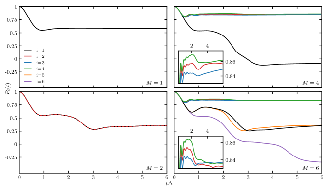
Figure 6: Population dynamics for each of the TLSs in a series of MSB models with varying numbers of TLSs coupled to a common heat bath. A bath containing 512 distinct frequencies is used in each case which correspond to baths containing 512, 1024, 2048, and 3072 bath modes for 1,2,4, and 6 TLSs, respectively. The inlays for the 4 and 6 spin cases, provide a closeup of the population dynamics for TLSs 2,3, and 4 all of which are located in a similar point in space.

We have considered the dynamics of four different MSB models with $M=$1, 2, 4, and 6 TLSs. The bath is discretized using 512 distinct frequencies, and as a consequence baths of 512, 1024, 3048, and 3072 modes are used for the 1, 2, 4, and 6 TLSs systems, respectively. The ML-MCTDH wavefunctions used in these calculations employed three groups of SPFs at the top level, one of which accounts for the degrees of freedom of the TLSs and includes as many SPFs as there are functions in the multi-TLS Hilbert space ($2^{M}$). The remaining two groups accounted for the bath degrees of freedom. The partitioning of bath modes uses the same procedure as used above for the spin-boson model, and employed two SPF groups for all subsequent layers. Simulations were performed with a range of different numbers of SPFs for treating the bath degrees of freedom, $N_{spf}$, however, in all cases twice as many functions ($2N_{spf})$ were used for the root node. The largest calculations considered here used $N_{spf}=100$. For the system with six TLSs this corresponds to expanding the wavefunction in terms of a basis of $2^{6}\times 200^{2}=2,560,000$ states at the top layer, and $100^{3}=1,000,000$ basis states for all other non-leaf layers. A total of $\sim 1.3\times 10^{9}$ variational parameters were used to parameterize the wavefunction. A primitive basis of 30 harmonic oscillator basis functions is used for each leaf node with frequency less than the bath cutoff frequency and 10 basis functions for all higher frequency modes. Mode combination was used with multiple physical modes being combined together up until a maximum Hilbert space dimension of 3000 was reached. All calculations presented in this section were performed with a time step of $dt\Delta=0.04$, unless otherwise specified, which was found sufficient to provide results converged to a relative cumulative deviation of $\sim\!10^{\text{{-}5}}$.

The results used as the reference calculations for each of the different MSB models are shown in Fig. 6. These calculations used $N_{spf}=48$, 80, 100, and 100 for $M=1$, 2, 4, and 6 TLSs, respectively. The dynamics obtained for the one TLS case are not particularly interesting; we see rapid initial decay of the population difference following which it plateaus to a finite value as the system is at sufficiently strong coupling that the dynamics are within the localised phase. For the two TLSs case, the population dynamics obtained for each TLS is identical due to symmetry. For short times the dynamics closely resembles that of the single TLS case, however, starting at around $t\Delta\sim 2.5$ the population difference begins to decay further before reaching a lower plateau at later times. This corresponds to the time required for propagation of phonons between the two TLSs, and so this further decay arises due to phonon mediated interactions between the TLSs. For the four and six TLSs cases, the population dynamics of TLSs 2, 3, and 4 are very similar (as shown in the insets). This arises due to the close proximity of these TLSs and thus the timescale on which the bath induces coupling between these TLSs is considerably faster than the timescale of the bath dynamics. In this regime, the bath-mediated interactions can be well described by a relatively strong, ferromagnetic, $\hat{{\sigma}}{}_{i,z}\hat{{\sigma}}{}_{j,z}$ coupling between the TLSs that results in strong correlations between the dynamics of these spins. At later times, these TLSs interact with the other TLSs present, and can result in significant changes in the population dynamics of the other spins due to the cumulative effect of the three spins.

$M$	1		2		4		6
$N_{spf}$	$\langle\Delta P\rangle$	$\langle N_{H}\rangle$	$\langle\Delta P\rangle$	$\langle N_{H}\rangle$	$\langle\Delta P\rangle$	$\langle N_{H}\rangle$	$\langle\Delta P\rangle$	$\langle N_{H}\rangle$
4	$3.5\times 10^{\text{-}3}$	$2.2\times 10^{3}$	$1.7\times 10^{\text{-}1}$	$2.1\times 10^{3}$	$1.2\times 10^{\text{-}1}$	$2.4\times 10^{3}$	$1.4\times 10^{\text{-}1}$	$2.4\times 10^{3}$
8	$3.8\times 10^{\text{-}4}$	$2.4\times 10^{3}$	$8.7\times 10^{\text{-}3}$	$2.3\times 10^{3}$	$5.5\times 10^{\text{-}2}$	$2.5\times 10^{3}$	$5.5\times 10^{\text{-}2}$	$2.5\times 10^{3}$
12	$4.0\times 10^{\text{-}5}$	$2.5\times 10^{3}$	$3.7\times 10^{\text{-}3}$	$2.3\times 10^{3}$	$3.0\times 10^{\text{-}2}$	$2.5\times 10^{3}$	$7.7\times 10^{\text{-}2}$	$2.5\times 10^{3}$
16	$8.1\times 10^{\text{-}6}$	$2.5\times 10^{3}$	$3.7\times 10^{\text{-}3}$	$2.4\times 10^{3}$	$2.4\times 10^{\text{-}2}$	$2.6\times 10^{3}$	$3.9\times 10^{\text{-}2}$	$2.5\times 10^{3}$
24	$2.7\times 10^{\text{-}6}$	$2.6\times 10^{3}$	$4.8\times 10^{\text{-}4}$	$2.6\times 10^{3}$	$1.0\times 10^{\text{-}2}$	$2.6\times 10^{3}$	$2.6\times 10^{\text{-}2}$	$2.7\times 10^{3}$
32	$1.3\times 10^{\text{-}6}$	$2.7\times 10^{3}$	$3.0\times 10^{\text{-}4}$	$2.6\times 10^{3}$	$6.0\times 10^{\text{-}3}$	$2.7\times 10^{3}$	$1.7\times 10^{\text{-}2}$	$2.6\times 10^{3}$
48	Reference	$3.8\times 10^{3}$	$4.9\times 10^{\text{-}5}$	$2.7\times 10^{3}$	$2.1\times 10^{\text{-}3}$	$3.2\times 10^{3}$	$1.1\times 10^{\text{-}2}$	$2.6\times 10^{3}$
64			$2.4\times 10^{\text{-}5}$	$2.8\times 10^{3}$	$1.5\times 10^{\text{-}3}$	$3.3\times 10^{3}$	$7.0\times 10^{\text{-}3}$	$2.7\times 10^{3}$
80			Reference	$2.9\times 10^{3}$	$7.1\times 10^{\text{-}4}$	$2.7\times 10^{3}$	$3.3\times 10^{\text{-}3}$	$2.7\times 10^{3}$
100					Reference	$3.3\times 10^{3}$	Reference	$2.7\times 10^{3}$

Table 5: Convergence of the population dynamics obtained for the MSB models with varying numbers of TLSs, $M$, as a function of the number of SPFs, $N_{spf}$. Convergence is measured through the average relative deviation of the population dynamics from reference calculations indicated in the table. We also present the average number of Hamiltonian evaluations per node required to obtain this dynamics out to a time $t\Delta=6$.

In order to accurately capture the dynamics of these systems, it is necessary to have enough SPFs that the correlations between individual TLSs and bath as well as the bath-mediated correlations between the TLSs can be well described. This becomes a more challenging problem as the number of TLSs increase, and as a result we find that significantly more SPFs are required to obtain accurate dynamics. In Table 5 we present the average relative deviations of the population dynamics of the systems and number of Hamiltonian applications required for varying numbers of SPFs. The number of Hamiltonian applications required for a given number of SPFs appears to be roughly independent of the number of TLSs considered. However there is a trend of requiring more Hamiltonian applications as the number of SPFs increases. This dependence is not very strong, with at most a factor of 2 increase being observed. As such, the increase in the number of Hamiltonian applications does not dramatically impact the computational effort associated with the calculations as the number of SPFs increase. It would be interesting to see whether this holds for the standard ML-MCTDH approach and improved schemes that employ regularization of singular mean-field density matrices. Whether the increase in the size of these mean-field density matrices due to an increase in the number of SPFs alters the size of the regularization parameter required to obtain converged results is not immediately obvious. Furthermore, whether the larger number of initially unoccupied SPFs increases the time over which the regularization impacts the dynamics remains to be seen.

The convergence of the population dynamics with respect to the number of SPFs differs considerably for systems with different numbers of TLSs. For the single TLS (spin-boson model) case, convergence is very rapid with deviations $<10^{\text{{-}4}}$ being obtained for $N_{spf}\geq 12$. As the number of TLSs increase it becomes considerably more challenging to converge dynamics. For the two TLSs case, a deviation $<10^{\text{{-}4}}$ is not obtained until $N_{spf}\geq 48$. Where as for the four and six TLSs case, the deviations between the population dynamics obtained for the largest numbers of SPFs ($N_{spf}=80$ and 100) are $7.1\times 10^{\text{-}4}$ and $3.3\times 10^{\text{-}3}$ , respectively. These relatively large deviations indicate that the dynamics are not fully converged with respect to the number of SPFs used. To give a more clear indication of the scale of these deviations, the population dynamics obtained for the four and six TLS models using $N_{spf}=64$, 80, and 100 are shown in Fig. 7.

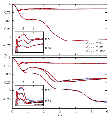
Figure 7: Convergence of the population dynamics with respect to the number of SPFs for $M=4$ (top) and 6 (bottom) TLSs. The population difference as a function of time for each TLS is shown. In each case, results were obtained using $N_{spf}=64$, 80, and 100 SPFs. The insets show a zoomed in view of the population difference dynamics for spins 2,3, and 4, which experience similar population dynamics.

For the four TLSs case, the population dynamics are converged to within the thickness of the lines shown when represented on the larger scale, however, some small deviations are observed in the population dynamics of TLSs 2,3, and 4 at times $t\Delta\geq 4$ (shown in the insets). For many applications, this level of convergence is sufficient. For the six TLSs case, more significant deviations are observed between the results with different numbers of SPFs, with the onset of these significant deviations being at shorter times $t\Delta\geq 1.5$. The timescale of the dynamics of TLSs 1, 5, and 6 is not fully converged, with the $N_{spf}=100$ case showing a slight shift to shorter times. In both cases, the results obtained with $N_{spf}=80$ agree with the results obtained using $N_{spf}=100$ to longer times than the results obtained $N_{spf}=64$, and show smaller deviations once they occur. In order to obtain fully converged results it would be necessary to consider even larger number of SPFs than have been considered here.

The primary factor limiting the number of SPFs that can be treated is the $\mathcal{{O}}(N_{spf}^{4})$ scaling of operations at each node, and $\mathcal{{O}}(N_{spf}^{3})$ scaling of the memory requirements. For reference, the six TLSs calculations with $N_{spf}=100$, required $\sim 32$ GB of memory to store the required data for the evolution. The memory limitations can be offset significantly through the use of out-of-core storage techniques. However, even with such techniques the size of systems that are practical to treat are still limited by the $\mathcal{{O}}(N_{spf}^{4})$ scaling of the number of operations applied to each node. The serial updating of nodes within the PSI limits the extent to which it can be parallelized. Only the linear algebra kernels applied in the evolution of each node can readily be parallelized. As a consequence, the wall time requirements can become very large for systems with larger numbers of SPFs. For reference, the six TLSs calculations with $N_{spf}=100$ took $\sim 480$ hours running on 8 cores of an Intel Xeon E5-2690 v3 CPU. For this case the speed up due to the use of parallelized linear algebra kernels was sublinear. However, it is likely that with further optimization better parallel performance could be obtained. This poor parallel performance arising from the serial nature of the node updates represents one of the main limitations of the current PSI approach.

Effect of Varying Timestep

$N_{spf}$	4	16	32	48
$dt\Delta$	$\langle\Delta P\rangle$
$6.4\times 10^{\text{-1}}$	$3.5\times 10^{\text{-}2}$	$6.7\times 10^{\text{-}3}$	$1.1\times 10^{\text{-}3}$	$4.6\times 10^{\text{-}4}$
$3.2\times 10^{\text{-1}}$	$1.6\times 10^{\text{-}2}$	$1.2\times 10^{\text{-}3}$	$2.4\times 10^{\text{-}4}$	$7.1\times 10^{\text{-}5}$
$1.6\times 10^{\text{-1}}$	$5.0\times 10^{\text{-}3}$	$5.6\times 10^{\text{-}4}$	$7.6\times 10^{\text{-}5}$	$1.4\times 10^{\text{-}5}$
$8\times 10^{\text{-2}}$	$2.5\times 10^{\text{-}3}$	$4.5\times 10^{\text{-}4}$	$5.3\times 10^{\text{-}5}$	$4.9\times 10^{\text{-}6}$
$4\times 10^{\text{-2}}$	$5.1\times 10^{\text{-}4}$	$4.0\times 10^{\text{-}4}$	$3.1\times 10^{\text{-}5}$	$4.4\times 10^{\text{-}6}$
$2\times 10^{\text{-2}}$	$2.8\times 10^{\text{-}4}$	$8.5\times 10^{\text{-}4}$	$3.2\times 10^{\text{-}5}$	$4.0\times 10^{\text{-}6}$
$1\times 10^{\text{-2}}$	$1.3\times 10^{\text{-}4}$	$5.4\times 10^{\text{-}4}$	$1.8\times 10^{\text{-}5}$	$2.1\times 10^{\text{-}6}$
$5\times 10^{\text{-3}}$	Reference	Reference	Reference	Reference

Table 6: Convergence of the population dynamics of the two TLS model with respect to time step for different numbers of SPFs. In each calculation the model parameters are as given in the main text. For each value of $N_{spf}$, convergence is measure with respect to a different reference, the calculation obtained with that value of $N_{spf}$ and with a time step of $dt\Delta=5\times 10^{\text{-3}}$.

As the number of SPFs increase, the deviation between results obtained with a given time step and the reference calculation obtained with a time step of $dt\Delta=5\times 10^{\text{-3}}$ decreases significantly. This result is readily understood when considering the approximations involved in obtaining the PSI. The PSI uses an expansion of the full wavefunction in terms of an orthonormal basis at each node of the tree. The evolution of the coefficient tensor at each node involves the construction of the propagator obtained from the projection of the Hamiltonian onto this local basis. As the size of this local basis increases, the projection of the Hamiltonian onto this basis better approximates the Hamiltonian in the full Hilbert space, and as a consequence the propagator evaluated using this projected Hamiltonian is accurate for longer times, and fewer Hamiltonian evaluations are required when integration the equations. In the limit of a complete basis expansion at each node of the tree, the propagator becomes exact and the approximation of a constant mean-field becomes exact for arbitrary times. These results further suggest that the projector splitting integrator could benefit significantly from an adaptive time step integration scheme. In particular, as the number of SPFs is increased such a scheme would be able to take larger time steps, potentially reducing the computational effort required to obtain converged results.

There is one additional point that we need to consider when discussing the convergence of the dynamics of this model. In principle, the dynamics should be converged with respect to the number of discrete bath modes, $M$, in order to reach the continuum bath limit. The memory and computer time requirements scale as $\mathcal{{O}}(M\log(M))$. Here, due to the large wall time requirements necessary to perform the calculations with large tree sizes and large number of SPFs we have restricted the bath to only 512 frequencies for the four and six TLSs cases. For the one and two TLSs cases, calculations using larger baths are feasible and are shown in Sec. VII.A of the Supplementary Information. Finally, as in the spin-boson model case, it is possible to perform a polaron transform for the MSB model. We have considered this in Sec. VII.B of the Supplementary Information for the one and two TLSs cases. These results show that, once again, the PSI has no issue when treating the challenging polaron-transformed representation.

IV Conclusion

In this paper we have discussed the implementation of the PSI for ML-MCTDH wavefunctions and have presented a series of numerical applications. Here, we have consider three different types of models:

• A two-dimensional, bi-linearly and bi-quadratically coupled harmonic oscillator model.

• A series of spin-boson models using both the standard and polaron-transformed forms of the Hamiltonian.

• A series of multi-spin-boson models.

These three types of models have allowed us to explore the stability and efficiency of the PSI in a number of different regimes.

The two-dimensional oscillator model serves as a useful test for how rank deficiency in the ML-MCTDH wavefunction influences the accuracy of the dynamics obtained by the PSI. The dynamics of unoccupied SPFs is arbitrary within any dynamical method that is based on linear variations, such as standard ML-MCTDH or the PSI. As a consequence, the dynamics of the wavefunction can depend on the value chosen for these unoccupied SPFs that do not initially contribute to the wavefunction. Here we find that while the dynamics obtained for this two-dimensional model can depend on the value of the initially unoccupied SPFs when 2 SPFs are used, uniformly sampling the initially unoccupied SPFs typically leads to dynamics that corresponds to the optimal choice of the initially unoccupied SPF. Further, if we increase the number of SPFs used to 3, then the results obtained do not depend on the initial choice of these functions. It is only when we have insufficient flexibility in the wavefunction to account for the two unoccupied SPFs that contribute significantly to the dynamics at short times that we find this dependence on initial conditions. While this two-dimensional model provides a convenient test case for the behavior of unoccupied SPFs it is not representative of the types of problems that ML-MCTDH would typically be applied to.

We next considered a series of spin-boson models that more closely resemble the types of problems that are typically treated using ML-MCTDH, and allow us to observe how the PSI performs for problems with considerably more modes. Converged dynamics were obtained for systems with up to $10^{6}$ degrees of freedom represented using tree structures with $\mathcal{O}(10^{5})$ nodes. By comparison with results that have previously been obtained using standard ML-MCTDH (and an improved variant) for systems with fewer modes,(Wang and Meyer, 2018, 2021) we find that the PSI approach provides an efficient and accurate approach. When compared to standard ML-MCTDH, we find that the PSI approach required between 3-4 orders of magnitude fewer Hamiltonian evaluations and 2-3 orders of magnitude fewer Hamiltonian applications in order to obtain well converged results. Even when compared to improved approaches, the PSI still demonstrated considerably better performance with up to a factor of 30 reduction in effort. When the polaron-transformed form of this model is considered, we find that a very small time step is required to obtain converged results. We show that this is due to large errors that occur during the first time step. The polaron-transformed Hamiltonian couples all modes together in a multiplicative fashion which leads to rapid initial evolution of the SPFs, and as a consequence the linearization is only accurate for short times. Motivated by this, we discuss a simple modification that while likely not optimal, considerably improves the convergence of the dynamics obtained using the PSI. This modification makes use of variable but not adaptive time steps with the goal of using smaller times steps to integrate the initial steps where large numbers of SPFs are unoccupied. Our results suggest that an adaptive time step integration scheme would be beneficial for the PSI. We have briefly discussed one such scheme that has previously been used for the MCTDH case and that we find is not generally useful for the multi-layer case.

Finally, we have considered a series of multi-spin-boson models that require considerably larger numbers of SPFs in order to obtain accurate results. We have presented results obtained using ML-MCTDH wavefunctions with up to 100 SPFs for each node and that contain a total of $1.3\times 10^{9}$ variational parameters. These results demonstrate that the PSI provides a stable approach even for ML-MCTDH wavefunctions that involve very large coefficient tensors. Furthermore, we find that as the number of SPFs increases, the approximations involved in the PSI become valid for longer times. As a consequence, the number of time steps required to accurately integrate the dynamics decreases as the representation of the wavefunction becomes more accurate.

We have identified two areas in which further development of this approach would be beneficial: adaptive time step control and parallelization of the algorithm. We have briefly discussed some efforts we have made towards addressing these issues and have pointed out the potential short comings of these approaches. Development in these areas remains an important area for future work. We believe that the results presented in this paper demonstrate that the PSI, even in its current form, is a robust and efficient approach for evolving ML-MCTDH wavefunctions, and that these results will encourage the implementation of such approaches within pre-existing ML-MCTDH packages. To help facilitate such development, the source code for the implementation of the PSI discussed here will be made available upon request.

Data Availability

The data that support the findings of this study are available from the corresponding author upon reasonable request.

References

- Manthe (2015a) U. Manthe, J. Chem. Phys. 142, 244109 (2015a).
- Meyer and Wang (2018) H.-D. Meyer and H. Wang, J. Chem. Phys. 148, 124105 (2018).
- Wang and Meyer (2018) H. Wang and H.-D. Meyer, J. Chem. Phys. 149, 044119 (2018).
- Weike and Manthe (2021) T. Weike and U. Manthe, J. Chem. Phys. 154, 194108 (2021).
- Manthe et al. (1992a) U. Manthe, H.-D. Meyer, and L. S. Cederbaum, J. Chem. Phys. 97, 3199 (1992a).
- Manthe et al. (1992b) U. Manthe, H.-D. Meyer, and L. S. Cederbaum, J. Chem. Phys. 97, 9062 (1992b).
- Manthe and Hammerich (1993) U. Manthe and A. D. Hammerich, Chem. Phys. Lett. 211, 7 (1993).
- Hammerich et al. (1994) A. D. Hammerich, U. Manthe, R. Kosloff, H.-D. Meyer, and L. S. Cederbaum, J. Chem. Phys. 101, 5623 (1994).
- Raab et al. (1999) A. Raab, G. Worth, H.-D. Meyer, and L. S. Cederbaum, J. Chem. Phys. 110, 936 (1999).
- Vendrell et al. (2007a) O. Vendrell, F. Gatti, D. Lauvergnat, and H.-D. Meyer, J. Chem. Phys. 127, 184302 (2007a).
- Vendrell et al. (2007b) O. Vendrell, F. Gatti, and H.-D. Meyer, J. Chem. Phys. 127, 184303 (2007b).
- Vendrell et al. (2009a) O. Vendrell, M. Brill, F. Gatti, D. Lauvergnat, and H.-D. Meyer, J. Chem. Phys. 130, 234305 (2009a).
- Vendrell et al. (2009b) O. Vendrell, F. Gatti, and H.-D. Meyer, J. Chem. Phys. 131, 034308 (2009b).
- Worth et al. (2008) G. A. Worth, H.-D. Meyer, H. Köppel, L. S. Cederbaum, and I. Burghardt, Int. Rev. Phys. Chem. 27, 569 (2008).
- Meng and Meyer (2013) Q. Meng and H.-D. Meyer, J. Chem. Phys. 138, 014313 (2013).
- Craig et al. (2007) I. R. Craig, M. Thoss, and H. Wang, J. Chem. Phys. 127, 144503 (2007).
- Wang and Thoss (2007) H. Wang and M. Thoss, J. Phys. Chem. A 111, 10369 (2007).
- I. et al. (2007) K. I., T. M., and W. H., J. Phys. Chem. C 111, 11970 (2007).
- Craig et al. (2011) I. R. Craig, M. Thoss, and H. Wang, J. Chem. Phys. 135, 064504 (2011).
- Borrelli et al. (2012) R. Borrelli, M. Thoss, H. Wang, and W. Domcke, Mol. Phys. 110, 751 (2012).
- Wilner et al. (2015) E. Y. Wilner, H. Wang, M. Thoss, and E. Rabani, Phys. Rev. B 92, 195143 (2015).
- Schulze et al. (2016) J. Schulze, M. F. Shibl, M. J. Al-Marri, and O. Kühn, J. Chem. Phys. 144, 185101 (2016).
- Shibl et al. (2017) M. F. Shibl, J. Schulze, M. J. Al-Marri, and O. Kühn, J. Phys. B 50, 184001 (2017).
- Mendive-Tapia et al. (2018) D. Mendive-Tapia, E. Mangaud, T. Firmino, A. de la Lande, M. Desouter-Lecomte, H.-D. Meyer, and F. Gatti, J. Phys. Chem. B 122, 126 (2018).
- (25) G. A. Worth, M. H. Beck, A. Jäckle, O. Vendrell, and H.-D. Meyer, “The mctdh package, version 8.2, (2000). h.-d. meyer, version 8.3 (2002),version 8.4 (2007). o. vendrell and h.-d. meyer version 8.5 (2013). version 8.5 contains the ml-mctdh algorithm. current versions: 8.4.20 and8.5.13 (2020). see http://mctdh.uni-hd.de/ for a description of the heidelberg mctdh package,” .
- Worth (2020) G. Worth, Comput. Phys. Commun. 248, 107040 (2020).
- Wang and Meyer (2021) H. Wang and H.-D. Meyer, J. Phys. Chem. A 125, 3077 (2021).
- Hinz et al. (2016) C. M. Hinz, S. Bauch, and M. Bonitz, J. Phys. Conf. Ser. 696, 012009 (2016).
- Mendive-Tapia and Meyer (2020) D. Mendive-Tapia and H.-D. Meyer, J. Chem. Phys. 153, 234114 (2020).
- Manthe (2015b) U. Manthe, J. Chem. Phys 142, 244109 (2015b).
- Lindoy (2019) L. Lindoy, New Developments in Open Quantum System Dynamics, Ph.D. thesis, Magdalen College, University of Oxford (2019).
- Schröder and Chin (2016) F. A. Schröder and A. W. Chin, Phys. Rev. B. 93, 29 (2016), arXiv:1507.02202 .
- Bauernfeind and Aichhorn (2020) D. Bauernfeind and M. Aichhorn, SciPost Phys. 8, 24 (2020).
- Kloss et al. (2020) B. Kloss, D. R. Reichman, and Y. B. Lev, SciPost Phys. 9, 70 (2020).
- Lubich (2014) C. Lubich, Appl. Math. Res. Express 2015, 311 (2014).
- Kloss et al. (2017) B. Kloss, I. Burghardt, and C. Lubich, J. Chem. Phys 146, 174107 (2017).
- Ceruti and Lubich (2021) G. Ceruti and C. Lubich, BIT Numer. Math. , 1 (2021).
- Goodrich and Tamassia (2010) M. T. Goodrich and R. Tamassia, Data Structures & Algorithms in Java, 5th ed. (John Wiley & Sons, 2010) p. 321.
- Ceruti et al. (2021a) G. Ceruti, C. Lubich, and H. Walach, SIAM J. Numer. Anal. 59, 289 (2021a).
- Kloss et al. (2018) B. Kloss, Y. Bar Lev, and D. Reichman, Phys. Rev. B 97, 024307 (2018).
- Paeckel et al. (2019) S. Paeckel, T. Köhler, A. Swoboda, S. R. Manmana, U. Schollwöck, and C. Hubig, Ann. Phys. (N. Y.) 411, 167998 (2019).
- Manthe (2018) U. Manthe, Chem. Phys. 515, 279 (2018).
- Larsson and Tannor (2017) H. R. Larsson and D. J. Tannor, J. Chem. Phys. 147, 044103 (2017).
- Yang and White (2020) M. Yang and S. R. White, Phys. Rev. B 102, 094315 (2020).
- Ceruti et al. (2021b) G. Ceruti, J. Kusch, and C. Lubich, arXiv preprint arXiv:2104.05247 (2021b).
- Garg et al. (1985) A. Garg, J. N. Onuchic, and V. Ambegaokar, J. Chem. Phys 83, 4491 (1985).
- Leggett et al. (1987) A. J. Leggett, S. Chakravarty, A. T. Dorsey, M. P. A. Fisher, A. Garg, and W. Zwerger, Rev. Mod. Phys. 59, 1 (1987).
- Nitzan (2006) A. Nitzan, Chemical Dynamics in Condensed Phases (Oxford University Press, 2006).
- Weiss (2012) U. Weiss, Quantum Dissipative Systems, 4th ed. (World Scientific Publishing Company, 2012).
- Wang et al. (2001) H. Wang, M. Thoss, and W. H. Miller, J. Chem. Phys. 115, 2979 (2001).
- Park and Light (1986) T. J. Park and J. C. Light, J. Comp. Phys. 85, 5870 (1986).
- Sidje (1998) R. B. Sidje, ACM Trans. Math. Softw. 24, 130 (1998).
- Orth et al. (2010) P. P. Orth, D. Roosen, W. Hofstetter, and K. Le Hur, Phys. Rev. B 82, 144423 (2010).
- McCutcheon et al. (2010) D. P. S. McCutcheon, A. Nazir, S. Bose, and A. J. Fisher, Phys. Rev. B 81, 235321 (2010).
- Winter and Rieger (2014) A. Winter and H. Rieger, Phys. Rev. B 90, 224401 (2014).
- Filippis et al. (2021) G. D. Filippis, A. de Candia, A. S. Mishchenko, L. M. Cangemi, A. Nocera, P. A. Mishchenko, M. Sassetti, R. Fazio, N. Nagaosa, and V. Cataudella, arXiv preprint arXiv:2103.16222 (2021).
- Joffrin and Levelut (1975) J. Joffrin and A. Levelut, J. Phys. (Paris) 36, 811 (1975).
- Kassner and Silbey (1989) K. Kassner and R. Silbey, J. Phys. Condens. Matter 1, 4599 (1989).
- Brown and Silbey (1998) F. L. H. Brown and R. J. Silbey, J. Chem. Phys. 108, 7434 (1998).
- Artiaco et al. (2021) C. Artiaco, F. Balducci, and A. Scardicchio, Phys. Rev. B 103, 214205 (2021).