Time Evolution of ML-MCTDH Wavefunctions I: Gauge Conditions, Basis Functions, and Singularities

Abstract

We derive a family of equations of motion (EOMs) for evolving multi-layer multiconfiguration time-dependent Hartree (ML-MCTDH) wavefunctions that, unlike the standard ML-MCTDH EOMs, never require the evaluation of the inverse of singular matrices. All members of this family of EOMs make use of alternative static gauge conditions than that used for standard ML-MCTDH. These alternative conditions result in an expansion of the wavefunction in terms of a set of potentially arbitrary orthonormal functions, rather than in terms of a set of non-orthonormal and potentially linearly dependent functions, as is the case for standard ML-MCTDH. We show that the EOMs used in the projector splitting integrator (PSI) and the invariant EOMs approaches are two special cases of this family obtained from different choices for the dynamic gauge condition, with the invariant EOMs making use of a choice that introduces potentially unbounded operators into the EOMs. As a consequence, all arguments for the existence of parallelizable integration schemes for the invariant EOMs can also be applied to the PSI EOMs.

I Introduction

The multiconfiguration time-dependent Hartree (MCTDH)(Meyer et al., 1990; Manthe et al., 1992a; Beck et al., 2000) and its multi-layer extension (ML-MCTDH)(Wang and Thoss, 2003; Manthe, 2008; Vendrell and Meyer, 2011; Wang, 2015) have found considerable success in obtaining systematically convergable dynamics for large quantum mechanical systems. Due to their general applicability, these approaches have been successfully employed to simulate the dynamics of small isolated systems (Manthe et al., 1992a, b; Manthe and Dell Hammerich, 1993; Hammerich et al., 1994; Raab et al., 1999; Vendrell et al., 2007a, b, 2009a, 2009b; Worth et al., 2008; Meng and Meyer, 2013) and considerably larger condensed-phase systems.(Craig et al., 2007; Wang and Thoss, 2007; Kondov et al., 2007; Craig et al., 2011; Borrelli et al., 2012; Wilner et al., 2015; Schulze et al., 2016; Shibl et al., 2017; Mendive-Tapia et al., 2018) As these approaches can, in principle, be converged to give the exact quantum dynamics, the results obtained using these techniques are also often used to benchmark other approaches.(Velizhanin et al., 2010; Liang et al., 2018; Laude et al., 2020) However, despite these successes there are regimes in which such approaches fail to capture the correct dynamics.(Hinz et al., 2016; Meyer and Wang, 2018; Wang and Meyer, 2018) One important cause for such difficulties is that the underlying equations-of-motion (EOMs) can become singular or nearly singular, necessitating the use of regularization techniques.(Beck et al., 2000) While regularization does not lead to significant numerical difficulties in many applications, in some cases regularization can dramatically influence the accuracy and efficiency of the approach, and these issues are not always easily detectable.(Meyer and Wang, 2018; Wang and Meyer, 2018; Weike and Manthe, 2021) Problems with regularization have been found to become more significant as the number of physical degrees of freedom in the system increases.(Wang and Meyer, 2021; Weike and Manthe, 2021) For the very large scale calculations that are now accessible these problems need to be addressed.

The singularity in the ML-MCTDH EOMs arises due to a fundamental issue associated with any approach that makes use of the ML-MCTDH ansatz, or more generally any tensor network representation which uses a time-dependent variational principle (TDVP) to obtain EOMs. Whenever the ML-MCTDH wavefunction is rank deficient, meaning that the exact wavefunction can be expressed using fewer expansion coefficients than are present in the ML-MCTDH wavefunction employed, the TDVP does not uniquely define the evolution of all coefficients in the ML-MCTDH wavefunction. In order to truly resolve this issue and obtain unique, non-singular EOMs, it is necessary to go beyond the linear variations employed within the TDVP. However, while approaches have been developed that use such techniques,(Manthe, 2015, 2018; Yang and White, 2020) they can involve considerably more effort than approaches based on linear variations.

Even if the ML-MCTDH wavefunction is not exactly rank deficient, it can often be nearly rank deficient during the early stages of the simulation. In the standard ML-MCTDH approach, this can lead to ill-conditioning of the EOMs, and it becomes necessary to regularize the EOMs. In challenging regimes, convergence with respect to the regularization parameter can be difficult to achieve, and this has motivated approaches that attempt to resolve this problem. One such approach that has found success in improving the stability of the ML-MCTDH EOMs makes use of an improved regularization scheme which leads to considerably more stable dynamics, and has allowed for dynamics to be obtained for models that are otherwise inaccessible via standard ML-MCTDH.(Meyer and Wang, 2018; Wang and Meyer, 2018, 2021)

An alternative means to alleviate the issues associated with rank deficiency and near rank deficiency involves the use of a different representation of the ML-MCTDH wavefunction, one in which the singularities that can be observed in the ML-MCTDH EOMs do not appear. Two approaches of this class are the invariant EOMs (Weike and Manthe, 2021) and the projector splitting integrator (PSI) method.(Lubich, 2015; Kieri et al., 2016; Kloss et al., 2017; Bonfanti and Burghardt, 2018; Ceruti et al., 2021) The PSI has found success in the simulation of the unitary dynamics of wavefunctions represented using Matrix Product States,(Schröder and Chin, 2016; Haegeman et al., 2016; Kloss et al., 2018; Paeckel et al., 2019) and the MCTDH (Kloss et al., 2017) and ML-MCTDH (Schröder et al., 2019; Kloss et al., 2020; Bauernfeind and Aichhorn, 2020; Ceruti et al., 2021) ansätze. The EOMs that are treated within this approach are non-singular regardless of whether the ML-MCTDH wavefunction is rank-deficient. However, this approach does not fundamentally resolve the issue associated with rank-deficiency of the ML-MCTDH wavefunction. In particular, rank-deficiency here manifests as non-uniqueness in the alternative representations that are used.(Meyer and Wang, 2018; Kloss et al., 2017) As a result, there have been questions raised within the ML-MCTDH community as to how well such an approach can work,(Manthe, 2015; Meyer and Wang, 2018) and there has been no general and systematic study of the relationship between these different representations or an understanding of the conditions for which individual approaches are optimal.

In this series of papers, we aim to address these concerns, and then demonstrate the tangible numerical benefits that arise from these considerations. In this work we will present a unified framework for deriving the ML-MCTDH EOMs, the PSI EOMs, and the invariant EOMs, as a means of clarifying the relationships between these approaches. In particular, we will discuss how the choice of gauge condition used within the standard ML-MCTDH approach results in an expansion of the wavefunction in terms of non-orthogonal and potentially linearly dependent sets of functions for all non-root nodes, giving rise to the singularities in the final EOMs. We will show that the PSI EOMs and invariant EOMs both make use of the same alternative representation in which the wavefunction is expanded in terms of a set of orthonormal but potentially arbitrarily selected functions. This is the source of the issues relating to the non-uniqueness of these approaches. These representations introduce an additional gauge freedom with respect to the standard ML-MCTDH EOMs from which we will derive the EOMs for generic dynamic gauge conditions, referred to as the Singularity Free EOMs. From this we will show that the PSI EOMs and invariant EOMs simply arise from different choices for this dynamic gauge condition. As such, the parallelizable integration scheme employed for the invariant EOMs(Weike and Manthe, 2021) can readily be extended to treat the PSI EOMs, and thus there is nothing inherent to the latter approach that restricts it to serial updates. However, in contrast to the PSI EOMs which are always non-singular, the choice for the dynamic gauge condition that is implicitly made in the original derivation of the invariant EOMs (and which we will make explicit) leads to singularities and therefore the need for regularization.

This paper is structured as follows. In Sec. II we will review the ML-MCTDH representation of the wavefunction and present the notation that will be used throughout. In Sec. III, we will present a derivation of the standard ML-MCTDH EOMs that considerably simplifies the process of arriving at singularity-free EOMs and provides a convenient intermediate point for obtaining singularity-free EOMs. In Sec. IV, we will present the alternative representation of the wavefunction that is used by the PSI and invariant EOMs, and by using this representation derive a set of EOMs that are free of singularities and describe the evolution of the full ML-MCTDH wavefunction. Some additional discussion of these EOMs is provided in the Supplementary Information. In Sec. V, we will discuss the invariant EOMs approach, and how it relates to the singularity-free EOMs. We will present our conclusions in Sec. VI.

In the companion paper we will aim to address concerns about the numerical performance of the approaches we advocate. We will discuss the implementation of the PSI for the ML-MCTDH wavefunction, with a focus on how the steps required relate to those required to implement standard ML-MCTDH. A series of applications of the PSI to models that represent significant challenges to standard ML-MCTDH, even when applying recently proposed improved regularization schemes, are then presented. These models will include a simple two-mode model that highlights the issue of rank deficient wavefunctions, a series of spin-boson models that have previously been considered with standard ML-MCTDH(Meyer and Wang, 2018; Wang and Meyer, 2018, 2021) using both standard and improved regularization schemes with baths containing up to $10^{6}$ bath modes, and a series of multi-spin-boson models that require considerably larger (in terms of size of coefficient tensors) ML-MCTDH wavefunctions to obtain converged results.

II The ML-MCTDH Wavefunction

In the ML-MCTDH approach, the high-dimensional time-dependent wavefunction $\left|\Psi(t)\right\rangle$ is expanded in terms of a basis constructed as a direct product of $d^{1}$ sets of “single-particle functions” (SPFs), $\left|\phi_{i}^{(1,k)}(t)\right\rangle$, as(Wang and Thoss, 2003; Manthe, 2008; Vendrell and Meyer, 2011)

$$\left|\Psi(t)\right\rangle=\sum_{i_{1}}^{n_{1}^{1}}\dots\sum_{i_{d^{1}}}^{n_{d^{1}}^{1}}A_{i_{1}\dots i_{d^{1}}}^{1}(t)\bigotimes_{k=1}^{d^{1}}\left|\phi_{i_{k}}^{(1,k)}(t)\right\rangle.$$ (1)

Each of these SPFs can then be expanded in terms of a direct product basis of $d^{(1,k)}$ sets of SPF for a further reduced subset of degrees of freedom. Applying this process recursively, each of the $N^{z_{l}}$ SPFs associated with a node can be expressed in terms of a direct product of SPFs as(Wang and Thoss, 2003; Manthe, 2008; Vendrell and Meyer, 2011)

$$\left|\phi_{i}^{z_{l}}(t)\right\rangle=\!\sum_{i_{1}}^{n_{1}^{z_{l}}}\!\dots\!\sum_{i_{d^{z_{l}}}}^{n_{d^{z_{l}}}^{z_{l}}}\!A_{i_{1}\dots i_{d^{z_{l}}}i}^{z_{l}}(t)\bigotimes_{k=1}^{d^{z_{l}}}\left|\phi_{i_{k}}^{(z_{l},k)}(t)\right\rangle,$$ (2)

where the label $z_{l}=(b_{1}\dots b_{l})$, contains the $l$ indices $b_{i}$ that denote the path required to reach this SPF starting from Eq. 1, and $d^{z_{l}}$ is the number of sets of SPFs forming the direct product basis. This process is repeated until at the bottom level the SPFs are expanded in terms of a primitive set of basis functions for the physical degrees of freedom of the system

$$\left|\phi_{i_{k}}^{(z_{l},k)}(t)\right\rangle=\Big{|}\chi_{\alpha}\Big{\rangle}.$$ (3)

From these definitions, the wavefunction can be expressed in terms of a series of contractions between the coefficient tensors, $A_{i_{1}\dots i_{d^{z}}i}^{z_{l}}(t)$. This process leads to a wavefunction that can be represented by a tree structure, as shown in Fig. 1, and is referred to as a tree tensor network. The coefficient tensors are represented as nodes of the tree, and contractions over indices common to two tensors are represented by lines linking the nodes. The ML-MCTDH wavefunction can, in principle, exactly represent an arbitrary wavefunction, and the accuracy of this expansion depends on the number of SPFs used at each node.

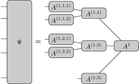
Figure 1: A diagram representing a ML-MCTDH approximation to a five-dimensional wavefunction. Each node of the tree corresponds to a coefficient tensor, and the lines connecting nodes represent the contraction over indices common to the two nodes.

Working with the individual coefficient tensors and SPFs becomes cumbersome for large tree structures. In order to simplify expressions it is useful to define the “single-hole functions” (SHFs), $\Psi_{i}^{z}$, associated with each node, $z$, by

$$\left|\Psi(t)\right\rangle=\sum_{i}^{N^{z_{l}}}\left|\phi_{\boldsymbol{}i}^{z_{l}}(t)\right\rangle\otimes\left|\Psi_{i}^{z_{l}}\right\rangle.$$ (4)

The definitions of the SPFs and SHFs are illustrated graphically in Fig. 2. In order to obtain a recursive definition for the SHFs that is consistent at all layers, including the first layer of the tree, we will define SHFs for the root node as the scalar function $\Psi_{1}^{1}(t)=1$ that acts on no physical degrees of freedom. Further, we will append an additional index $i=1$ to the root node coefficient tensor such that $A^{1}_{1_{1}\dots i_{d^{1}}i}\equiv A^{1}_{1_{1}\dots i_{d^{1}}}$, and define the number of SPFs at the root nodes as $N^{1}=1$. Using this notation, the SHFs of any node $(z_{l},k)$ can be obtained recursively in terms of the coefficient tensor and SHFs of its parent node, $z_{l}$, and the SPFs of the sibling nodes of node $(z_{l},k)$ (that is all nodes $(z_{l},j)$ with $j\neq k$) by

$$\Big{|}\Psi_{n}^{(z_{l},k)}(t) \Big{\rangle}=\!\sum_{i_{1}}^{n_{1}^{z_{l}}}\!\dots\!\sum_{i_{k-1}}^{n_{k-1}^{z_{l}}}\!\sum_{i_{k+1}}^{n_{k+1}^{z_{l}}}\!\dots\!\sum_{i_{d^{z_{l}}}}^{n_{d^{z_{l}}}^{z_{l}}}\sum_{m=1}^{N^{z_{l}}}\left|\Psi_{m}^{z_{l}}(t)\right\rangle\cdot$$ (5)

$$A_{i_{1}\dots i_{k-1}ni_{k+1}\dots i_{d^{z_{l}}}m}^{z_{l}}\left(\bigotimes_{\begin{subarray}{c}j=1\\ {j\neq k}\end{subarray}}^{d^{z_{l}}}\left|\phi_{i_{j}}^{(z_{l},j)}(t)\right\rangle\right).$$

While the SPFs are required to be orthonormal, $\left.\left\langle\phi_{\boldsymbol{}i}^{z_{l}}(t)\right|\phi_{\boldsymbol{}j}^{z_{l}}(t)\right\rangle=\delta_{ij}\ \forall\ z_{l}$, this is not the case for the SHFs constructed using Eq. 5. Instead, we generate an overlap matrix, $\rho_{ij}^{z_{l}}=\left.\left\langle\Psi_{i}^{z_{l}}(t)\right|\Psi_{j}^{z_{l}}(t)\right\rangle$, which is referred to as the mean-field density matrix of node $z_{l}$. This matrix can become singular whenever the SHFs are linearly dependent, a situation that is often encountered during the early stage of simulations when separable or weakly entangled initial condition are used. As will be discussed later, this leads to significant numerical issues in the evolution of ML-MCTDH wavefunctions.

Using the recursive definition of the SPFs, we may expand the full wavefunction as

$$\left|\Psi(t)\right\rangle \!=\!\sum_{i_{1}}^{n_{1}^{z_{l}}}\!\dots\!\sum_{i_{d^{z_{l}}}}^{n_{d^{z_{l}}}^{z_{l}}}\!\sum_{i}^{N^{z_{l}}}\!A_{i_{1}\dots i_{d^{z_{l}}}i}^{z_{l}}(t)\left|\Psi_{i}^{z_{l}}(t)\right\rangle\!\otimes\!\left(\!\bigotimes_{k=1}^{d^{z_{l}}}\!\left|\phi_{i_{k}}^{(z_{l},k)}(t)\!\right\rangle\!\right)$$ (6)

$$=\!\!\!\!\!\sum_{I^{z_{l}}}^{n_{1}^{z_{l}}\dots n_{d^{z_{l}}}^{z_{l}}}\!\sum_{i}^{n^{z_{l}}}A_{I^{z_{l}}i}^{z_{l}}(t)\left|\Psi_{i}^{z_{l}}(t)\right\rangle\!\otimes\!\left|\Phi_{I^{z_{l}}}^{z_{l}}(t)\right\rangle,$$

where $I^{z_{l}}=(i_{1},\dots,i_{d^{z}})$ is a combined index for all indices involved in the contractions with the children of node $z_{l}$, and $\left|\Phi_{I^{z_{l}}}^{z_{l}}(t)\right\rangle$ is the direct product of the SPFs associated with the children of node $z_{l}$, which we will refer to as the configurations of node $z_{l}$ in the following. This corresponds to an expansion of the wavefunction in terms of the (time-dependent) direct product of the SPFs associated with the children of node $z_{l}$ and SHFs associated with node $z_{l}$, where the tensor $A_{I^{z_{l}}i}^{z_{l}}(t)$ contains the expansion coefficients. In what follows we will prefer to work with a matrix representation of the states, and so we will now expand the wavefunction in terms of the primitive basis. Doing so gives the following expression for the elements of the wavefunction coefficient tensor

$$\Psi_{\alpha^{z_{l}}\beta^{z_{l}}}(t) =\!\!\!\!\!\sum_{I^{z_{l}}}^{n_{1}^{z_{l}}\dots n_{d^{z_{l}}}^{z_{l}}}\!\sum_{i}^{n^{z_{l}}}A_{I^{z_{l}}i}^{z_{l}}(t)\Phi_{\alpha^{z_{l}}I^{z_{l}}}^{z_{l}}(t)\Psi_{i\beta^{z_{l}}}^{z_{l}}(t)$$ (7)

$$=\left[\boldsymbol{{\Phi}}^{z_{l}}(t)\boldsymbol{{A}}^{z_{l}}(t)\boldsymbol{{\Psi}}^{z_{l}}(t)\right]_{\alpha^{z_{l}}\beta^{z_{l}}},$$

where $\alpha^{z_{l}}$ and $\beta^{z_{l}}$ are sets of indices for the physical degrees of freedom of SPFs and SHFs associated with node $z_{l}$, respectively. In order to use this notation for all nodes, we will make use of the definition of the SHFs for the root nodes given above, and for the leaf nodes we will define the configurations coefficient tensor to be $\boldsymbol{{\Phi}}^{z_{l}}(t)=\boldsymbol{{I}}$. In the final line we have written this using a matrix representation for all of the tensors present.

This representation is particularly useful when evaluating the ML-MCTDH EOMs, as it directly provides access to the coefficient tensors that we seek to evolve. However, this representations is not unique. It is possible to insert any pair of time-dependent matrices of the correct sizes that multiply to give the identity matrix between any of the matrices in Eq. 7, e.g.

$$\Psi_{\!\alpha^{z_{l}}\!\beta^{z_{l}}}\!(t)\!= \!\Big{[}\boldsymbol{{\Phi}}^{z_{l}}(t)\boldsymbol{{X}}(t)\boldsymbol{{X}}^{\text{{-}1}}(t)\boldsymbol{{A}}^{z_{l}}(t)\boldsymbol{{Y}}(t)\boldsymbol{{Y}}^{\text{{-}1}}(t)\boldsymbol{{\Psi}}^{z_{l}}(t)\Big{]}_{\!\alpha^{z_{l}}\!\beta^{z_{l}}}$$ (8)

$$= \!\Big{[}\boldsymbol{{\Phi}}^{\prime z_{l}}(t)\boldsymbol{{A}}^{\prime z_{l}}(t)\boldsymbol{{\Psi}}^{\prime z_{l}}(t)\Big{]}_{\!\alpha^{z_{l}}\!\beta^{z_{l}}}.$$

In order to remove this gauge freedom, it is necessary to specify some additional conditions, namely the static and dynamic gauge conditions.

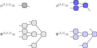
Figure 2: Diagram representing the SPFs and SHFs associated with different nodes of the ML-MCTDH wavefunction shown in Fig. 1. Here we have dropped the labels of the coefficient tensors in the tree tensor network. The entire wavefunction can be constructed by contracting together the SPF and SHF tensors for a given node.

III The ML-MCTDH Equations of Motion

In order for the ML-MCTDH approach to be efficient, it is necessary to be able to efficiently evaluate the action of the Hamiltonian on the ML-MCTDH wavefunction. One representation that is particularly useful for the ML-MCTDH approach is the sum-of-product (SOP) form of the Hamiltonian, in which the Hamiltonian is expressed as a sum of terms, with each term expressed as a direct product of operators acting on the physical modes of the system. For a Hamiltonians in this SOP form, we may write

$$\hat{{H}}=\sum_{r}\hat{{h}}_{r}^{z_{l}}\hat{{H}}_{r}^{z_{l}},$$ (9)

where we have partitioned each of the product operators into a direct product of terms $\hat{{h}}_{r}^{z_{l}}$ that act on the physical degrees of freedom accounted for by the configurations, and terms $\hat{{H}}_{r}^{z_{l}}$ that act on the physical degrees of freedom accounted for by the SHF basis associated with node $z_{l}$. For the root node, the mean-field Hamiltonians will be taken as the scalar $\hat{{H}}_{r}^{1}=1$.

The standard ML-MCTDH approach removes this ambiguity by requiring that for each node the SPFs are orthonormal and remain orthonormal through the evolution. This can be done by imposing orthonormality of the SPFs at a given time, which amounts to a static gauge condition. However on its own this condition is not sufficient to remove all ambiguities in this representation. It is still possible to insert arbitrary unitary factors (and their inverses) between terms. This ambiguity can be removed by enforcing a dynamic gauge condition on the SPFs associated with each of the non-root nodes $z_{l}$(Beck et al., 2000; Wang and Thoss, 2003; Manthe, 2008)

$$\boldsymbol{{\phi}}^{z_{l}\dagger}(t)\dot{{\boldsymbol{{\phi}}}}{\!\;\!}^{z_{l}}(t)=-\boldsymbol{{i}}\boldsymbol{{x}}^{z_{l}}(t),$$ (10)

where $\boldsymbol{{x}}^{z_{l}}(t)$ is a Hermitian matrix for all times that can, in general, depend on the ML-MCTDH wavefunction. The choice of the matrix $\boldsymbol{{x}}^{z_{l}}(t)$ does not effect the accuracy of the ML-MCTDH approach, however, it can influence the numerical efficiency of the integration of the final EOMs.

As the SPFs can be expanded in terms of the coefficient tensor and SPFs of the children of node $z_{l}$,

$$\boldsymbol{{\phi}}^{z_{l}}(t)=\left(\bigotimes_{k=1}^{d^{z_{l}}}\boldsymbol{{\phi}}^{(z_{l},k)}(t)\right)\boldsymbol{{A}}^{z_{l}}(t)=\boldsymbol{{\Phi}}^{z_{l}}(t)\boldsymbol{{A}}^{z_{l}}(t),$$ (11)

it can readily be shown that these gauge conditions apply constraints to all non-root coefficient tensors. The gauge condition (Eq. 10) for each of the SPFs of the children node $z_{l}$ leads to the following constraint on the coefficient tensors for the configurations,

$$\boldsymbol{{\Phi}}^{z_{l}\dagger}(t)\dot{{\boldsymbol{{\Phi}}}}{\!\;\!}^{z_{l}}(t)=-\boldsymbol{{i}}\left(\bigoplus_{k=1}^{d^{z_{l}}}\boldsymbol{{x}}^{(z_{l},k)}(t)\right)=-\boldsymbol{{i}}\boldsymbol{{X}}^{z_{l}}(t),$$ (12)

where $\bigoplus_{k}$ denotes a direct sum over matrices indexed by $k$. As such, the coefficient tensors are constrained to satisfy

$$\boldsymbol{{A}}^{z_{l}\dagger}(t)\dot{\boldsymbol{{A}}}{\!\;\!}^{z_{l}}(t)=-i\boldsymbol{{x}}^{z_{l}}(t)+i\boldsymbol{{A}}^{z_{l}\dagger}(t)\boldsymbol{{X}}^{z_{l}}(t)\boldsymbol{{A}}^{z_{l}}(t).$$ (13)

These conditions ensure that the configurations remain orthonormal and that the coefficient matrix remains semi-unitary for all time. As a consequence, any non-orthonormality associated with the matrix expansion of the wavefunction given in Eq. 7 must be accounted for by the SHF coefficient tensor. Thus the standard ML-MCTDH approach expands the wavefunction at each (non-root) node in terms of a direct product of orthonormal SPFs and non-orthonormal, and in some cases linearly dependent, SHFs with an expansion coefficient matrix that is semi-unitary.

With these constraints and the specification of the Hamiltonian we are now in a position to derive the ML-MCTDH EOMs. The standard derivation of the ML-MCTDH EOMs has been presented in a number of places,(Wang and Thoss, 2003; Manthe, 2008) here we will present a slightly different path to the final ML-MCTDH EOMs. In the derivation that follows, all matrices and states are time-dependent. However, in order to prevent the equations becoming too cumbersome, we will not indicate this explicitly in intermediate equations. As is standard, we begin by applying the Dirac-Frenkel variational principle(Wang and Thoss, 2003; Manthe, 2008)

$$\big{\langle}\delta\Psi\big{|}i\frac{{\partial}}{\partial t}-\hat{{H}}\big{|}\Psi\big{\rangle}=0$$ (14)

to the ML-MCTDH wavefunction. The variation of the wavefunction can be written in the form(Manthe, 2008)

$$\big{|}\delta\Psi\big{\rangle}=\sum_{z_{l}\in\Psi}\sum_{I^{z_{l}}}\sum_{i^{z_{l}}}\delta A_{I^{z_{l}}i^{z_{l}}}^{z_{l}}\big{|}\Phi_{I^{z_{l}}}^{z_{l}}\big{\rangle}\otimes\big{|}{\Psi_{i^{z_{l}}}^{z_{l}}}\big{\rangle}.$$ (15)

Inserting this into the Dirac-Frenkel variational principle, we have

$$\sum_{z_{l}\in\Psi}\sum_{I^{z_{l}}}\sum_{i^{z_{l}}}\delta A_{I^{z_{l}}i^{z_{l}}}^{z_{l}\dagger}\big{\langle}\Phi_{I^{z_{l}}}^{z_{l}}\big{|}\otimes\big{\langle}\Psi_{i^{z_{l}}}^{z_{l}}\big{|}i\frac{{\partial}}{\partial t}-\hat{{H}}\left|\Psi\right\rangle=0.$$ (16)

The variations of the coefficient tensors $\delta A_{I^{z_{l}}i^{z_{l}}}^{z_{l}\dagger}$ are independent, and we can therefore consider variations of each of the coefficient tensors independently. Doing so simplifies this expression to give

$$\sum_{I^{z_{l}}}\sum_{i^{z_{l}}}\delta A_{I^{z_{l}}i^{z_{l}}}^{z_{l}\dagger}\big{\langle}\Phi_{I^{z_{l}}}^{z_{l}}\big{|}\otimes\big{\langle}\Psi_{i^{z_{l}}}^{z_{l}}\big{|}i\frac{{\partial}}{\partial t}-\hat{{H}}\big{|}\Psi\big{\rangle}=0,$$ (17)

where now we are only considering variations of the coefficient tensor of node $z_{l}$. We can now expand the time derivative of the wavefunction using the representation of the wavefunction given in Eq. 6, which yields

$$\left|\dot{\Psi}\right\rangle= \sum_{J^{z_{l}}}\sum_{j}\Big{(}\dot{A}{}_{J^{z_{l}}j}^{z_{l}}\left|\Phi_{J^{z_{l}}}^{z_{l}}\right\rangle\left|\Psi_{j}^{z_{l}}\right\rangle$$ (18)

$$+ A_{J^{z_{l}}j}^{z_{l}}\big{|}\dot{{\Phi}}_{J^{z_{l}}}^{z_{l}}\big{\rangle}\big{|}\Psi_{j}^{z_{l}}\big{\rangle}+A_{J^{z_{l}}j}^{z_{l}}\big{|}\Phi_{J^{z_{l}}}^{z_{l}}\big{\rangle}\big{|}\dot{\Psi}_{j}^{z_{l}}\big{\rangle}\Big{)}.$$

Inserting this expression into Eq. 17, and noting that the resultant expression holds for all allowed variations of the coefficient tensor, we may equate coefficients to remove the dependence on the variations. This yields an equation that can be written in terms of the configurations and SHF and node coefficient matrices as

$$\boldsymbol{\Phi}^{z_{l}\dagger}\dot{{\boldsymbol{{\Phi}}}}{\!\;\!}^{z_{l}}\boldsymbol{{A}}^{z_{l}}\boldsymbol{{\Psi}}^{z_{l}}\boldsymbol{{\Psi}}^{z_{l}\dagger}+\boldsymbol{\Phi}^{z_{l}\dagger}\boldsymbol{\Phi}^{z_{l}}\dot{{\boldsymbol{{A}}}}{\!\;\!}^{z_{l}}\boldsymbol{{\Psi}}^{z_{l}}\boldsymbol{{\Psi}}^{z_{l}\dagger}$$ (19)

$$+\boldsymbol{\Phi}^{z_{l}\dagger}\boldsymbol{\Phi}^{z_{l}}\boldsymbol{{A}}^{z_{l}}\dot{{\boldsymbol{{\Psi}}}}{\!\;\!}^{z_{l}}\boldsymbol{{\Psi}}^{z_{l}\dagger}=-\frac{{i}}{\hbar}\sum_{r}\boldsymbol{{h}}_{r}^{z_{l}}\boldsymbol{{A}}^{z_{l}} \boldsymbol{{H}}_{r}^{z_{l}}.$$

Here we have used the sum-of-product representation of the Hamiltonian, and we have introduced the SPF, $\boldsymbol{{h}}_{r}^{z_{l}}$(t), and mean-field, $\boldsymbol{{H}}_{r}^{z_{l}}(t)$, Hamiltonian matrices, respectively. These Hamiltonians have the matrix elements

$$\left[\boldsymbol{{h}}_{r}^{z_{l}}(t)\right]_{IJ} =\left\langle\Phi_{I}^{z_{l}}(t)\right|\hat{h}_{r}^{z_{l}}\left|\Phi_{J}^{z_{l}}(t)\right\rangle,$$ (20)

$$\left[\boldsymbol{{H}}_{r}^{z_{l}}(t)\right]_{ij} =\left\langle\Psi_{i}^{z_{l}}(t)\right|\hat{H}_{r}^{z_{l}}\left|\Psi_{j}^{z_{l}}(t)\right\rangle.$$ (21)

The SPF and mean-field Hamiltonian matrices depend on all coefficient tensors used to evaluate the configurations and SHFs for node $z_{l}$, respectively. Here for notational simplicity we will not explicitly indicate this dependence.

For the root node, we can apply the gauge conditions for the SPFs, use the fact that the SPF coefficient tensor is semi-unitary, and make use of the fact that we have defined the SHFs as a time-independent scalar to obtain(Beck et al., 2000; Wang and Thoss, 2003; Manthe, 2008)

$$\dot{{\boldsymbol{{A}}}}{\!\;\!}^{1}(t)=-i\left(\frac{1}{\hbar}\boldsymbol{{h}}{}^{1}(t)-\boldsymbol{{X}}^{1}(t)\right)\boldsymbol{{A}}^{1}(t).$$ (22)

For a given non-root node $z_{l}$, applying the gauge conditions for the SPFs simplifies Eq. 19, giving

$$-\boldsymbol{{X}}^{z_{l}}(t)\boldsymbol{{A}}^{z_{l}}\boldsymbol{{\rho}}^{z_{l}}+\dot{\boldsymbol{A}}{\!\;\!}^{z_{l}}\boldsymbol{{\rho}}^{z_{l}}$$ (23)

$$+\boldsymbol{{A}}^{z_{l}}\dot{{\boldsymbol{{\Psi}}}}^{z_{l}}\boldsymbol{{\Psi}}^{z_{l}\dagger}=-\frac{{i}}{\hbar} \sum_{r}\boldsymbol{{h}}_{r}^{z_{l}}\boldsymbol{{A}}^{z_{l}}\boldsymbol{{H}}_{r}^{z_{l}},$$

where $\boldsymbol{{\rho}}^{z_{l}}=\boldsymbol{\Psi}^{z_{l}}\boldsymbol{\Psi}^{z_{l}\dagger}$ is the mean-field density matrix discussed previously, which like the mean-field Hamiltonian depends on the coefficient tensors of all nodes used in the evaluation of the SHFs. This equation describes the evolution of both the coefficient tensor associated with a node as well as the SHF coefficient tensors, and thus all of the coefficient tensors of nodes used to define the SHF coefficient tensors.

It is possible to arrive at the EOMs for the coefficient tensor of node $z_{l}$ by expanding the derivative of the SHF coefficient tensor using the recursive expression for the SHF coefficient tensors, as is the standard approach taken in arriving at the ML-MCTDH EOMs.(Wang and Thoss, 2003) However, this is a relatively cumbersome task. An alternative and considerably faster approach simply involves applying the projector

$$\boldsymbol{{Q}}^{z_{l}}=\boldsymbol{{I}}-\boldsymbol{{A}}^{z_{l}}\boldsymbol{{A}}^{z_{l}\dagger}=\boldsymbol{I}-\boldsymbol{P}^{z_{l}},$$ (24)

where $\boldsymbol{{I}}$ is the identity matrix, to Eq. 23 from the left. This projector acts on the matrix $\boldsymbol{{A}}^{z_{l}}$ to give

$$\boldsymbol{{Q}}^{z_{l}}\boldsymbol{{A}}^{z_{l}}=\boldsymbol{A}^{z_{l}}-\boldsymbol{{A}}^{z_{l}}\boldsymbol{{A}}^{z_{l}\dagger}\boldsymbol{{A}}^{z_{l}}=\boldsymbol{{0}},$$ (25)

due to the semi-unitarity of the coefficient tensors. As such, the term containing the derivative of the SHF vanishes when this projector is applied. Using these facts we find

$$-\boldsymbol{{Q}}^{z_{l}}\boldsymbol{{X}}^{z_{l}}(t)\boldsymbol{{A}}^{z_{l}}\boldsymbol{{\rho}}^{z_{l}}+\dot{{\boldsymbol{{A}}}}{\!\;\!}^{z_{l}}\boldsymbol{{\rho}}^{z_{l}}$$ (26)

$$-\boldsymbol{{A}}^{z_{l}}\boldsymbol{{A}}^{z_{l}\dagger}\dot{{\boldsymbol{{A}}}}{\!\;\!}^{z_{l}}\boldsymbol{{\rho}}^{z_{l}}=-\frac{{i}}{\hbar}\boldsymbol{{Q}}^{z_{l}} \sum_{r}\boldsymbol{{h}}_{r}^{z_{l}}\boldsymbol{{A}}^{z_{l}}\boldsymbol{{H}}_{r}^{z_{l}}.$$

Inserting Eq. 13 and rearranging terms gives the final ML-MCTDH EOMs for all non-root nodes(Wang and Thoss, 2003; Manthe, 2008)

$$\dot{{\boldsymbol{{A}}}}{\!\;\!}^{z_{l}}(t)\!= -\frac{{i}}{\hbar}\boldsymbol{{Q}}^{z_{l}}(t)\!\sum_{r}\!\boldsymbol{{h}}_{r}^{z_{l}}(t)\boldsymbol{{A}}^{z_{l}}(t)\boldsymbol{{H}}_{r}^{z_{l}}(t)\boldsymbol{{\rho}}^{z_{l}}(t)^{-1}$$ (27)

$$-i\boldsymbol{{A}}^{z_{l}}(t)\boldsymbol{{x}}^{z_{l}}(t)+i\boldsymbol{{X}}^{z_{l}}(t)\boldsymbol{{A}}^{z_{l}}(t).$$

This expression contains the inverse of the mean-field density matrix (the SHF overlap matrix). Whenever the SHFs are linearly dependent, the mean-field density matrix becomes singular and its inverse ill-defined. This in turn leads to ill-defined ML-MCTDH EOMs, as they require the evaluation and application of an unbounded operator. When the SHFs are nearly linearly dependent, the condition number of the mean-field density matrix becomes large, and the ML-MCTDH EOMs for the SPFs can become very stiff, significantly increasing the computation effort required for integration. In such cases, the ML-MCTDH EOMs can lead to rapid evolution of the coefficient tensors, giving rise to a rapid evolution of the weakly occupied SPFs.(Wang and Meyer, 2018) In practice it is necessary to regularize the inverse of the mean-field density matrix when evaluating the EOMs. A number of different strategies have been developed to regularize these equations, however in all cases they introduce a bias into the equations, and it becomes necessary to converge the dynamics with respect to this bias. For many problems, moderate levels of regularization do not significantly alter the dynamics and it is possible to obtain dynamics that are converged with respect to the regularization parameter. However, for some problems small regularization parameters may be required to obtain accurate dynamics. As the inverse of the standard regularization parameter is directly related to the condition number of the regularized inverse of the mean-field density matrix, small regularization parameters correspond to increased computation effort. In severe cases, this may even prevent converged dynamics from being obtained.

Before one can solve the ML-MCTDH EOMs, it is necessary to specify the constraint matrices. The standard choice for this constraint matrix is(Wang and Thoss, 2003; Beck et al., 2000; Manthe, 2008)

$$\boldsymbol{{x}}^{z_{l}}(t)=\boldsymbol{0}.$$ (28)

This choice minimises the motion of configurations, and is particularly useful when using constant mean-field integration (CMF) schemes discussed in Sec. I.A of the Supplementary Information. Alternative choices for the dynamic gauge condition may lead to numerical benefits in some situations.(Wang and Thoss, 2003; Beck et al., 2000; Manthe, 2008)

IV Singularity-Free Equations of Motion

As discussed in the previous section, the singularities present in the ML-MCTDH EOMs arise due to the use of a non-orthonormal set of SHFs in the expansion of the wavefunction. It is therefore reasonable to ask whether the use of orthonormalized SHFs will lead to non-singular EOMs. Here we will demonstrate that such a choice leads to a family of singularity-free EOMs that differ in the choice of their gauge conditions, and demonstrate that the PSI EOMs arise from one such gauge choice. In order to explore this we consider an alternative expansion of the full wavefunction than that given by Eq. 7, one in which the SHF basis functions are orthonormal.

To construct such a representation, we will make use of the following decomposition of the SHF coefficient matrix for the non-root node $z_{l}$

$$\boldsymbol{{\Psi}}^{z_{l}}(t)=\boldsymbol{{R}}^{z_{l}}(t)\widetilde{{\boldsymbol{{\Psi}}}}{\!\;\!}^{z_{l}}(t),$$ (29)

where $\widetilde{{\boldsymbol{{\Psi}}}}{\!\;\!}^{z_{l}}$ is a semi-unitary matrix defining an orthonormal set of SHFs represented in terms of the primitive basis, and $\boldsymbol{{R}}^{z_{l}}$ contains the expansion coefficients of the old SHF in terms of these new functions. While a decomposition of this form can be performed for any matrix, this will in general be impractical for the full expanded SHF coefficient matrix due to its large size. In practice, a recursive approach is used for constructing this decomposition that makes use of the definition of the SHFs given in Eq. 5. Such a strategy allows for the construction of a tree tensor network representation of the transformed SHF coefficient tensor, which is necessary for practical applications of the approach.

The wavefunction can be expanded in terms of the standard configurations and the new SHF states at node $z_{l}$ as

$$\left|\Psi(t)\right\rangle =\!\!\!\!\!\!\sum_{I^{z_{l}}}^{n_{1}^{z_{l}}\dots n_{d^{z_{l}}}^{z_{l}}}\!\sum_{i,j}^{n^{z_{l}}}\!A_{I^{z_{l}}i}^{z_{l}}(t)\left|\Phi_{I^{z_{l}}}^{z_{l}}(t)\right\rangle\!\otimes\!R_{ij}^{z_{l}}(t)\!\left|\widetilde{\Psi}{\!\;\!}_{j}^{z_{l}}(t)\!\right\rangle$$ (30)

$$=\!\!\!\!\!\!\sum_{I^{z_{l}}}^{n_{1}^{z_{l}}\dots n_{d^{z_{l}}}^{z_{l}}}\!\sum_{j}^{n^{z_{l}}}\widetilde{A}{\!\;\!}_{I^{z_{l}}j}^{z_{l}}(t)\left|\Phi_{I^{z_{l}}}^{z_{l}}(t)\right\rangle\!\otimes\!\left|\widetilde{\Psi}{\!\;\!}_{j}^{z_{l}}(t)\!\right\rangle.$$

Here we have introduced the transformed coefficient tensors $\widetilde{A}{\!\;\!}_{\boldsymbol{{I}}j}^{z_{l}}(t)$ which are related to the standard coefficient tensors by the matrix expression

$$\widetilde{{\boldsymbol{{A}}}}{\!\;\!}^{z_{l}}(t)=\boldsymbol{{A}}^{z_{l}}(t)\boldsymbol{{R}}^{z_{l}}(t).$$ (31)

We can also express the wavefunction in terms of the new SHF states and the original SPF states for the non-root node $z_{l}$ as

$$\left|\Psi(t)\right\rangle =\sum_{i,j}^{n^{z_{l}}}R_{ij}^{z_{l}}(t)\big{|}\phi_{i}^{z_{l}}(t)\big{\rangle}\otimes\big{|}\widetilde{\Psi}{\!\;\!}_{j}^{z_{l}}(t)\big{\rangle}.$$ (32)

In contrast to Eq. 6, both of the wavefunction expressions immediately above correspond to an expansion in terms of an incomplete but orthonormal set of functions. For the root node, the original representation already corresponds to an expansion of the wavefunction in terms of an orthonormal set of functions as there are no SHFs associated with the root. As such, we use the standard representation, and for simplicity we will define $\widetilde{{\boldsymbol{{A}}}}{\!\;\!}^{1}(t)\equiv\boldsymbol{{A}}^{1}(t).$ Note we have not introduced a set of transformed SHFs for the root node or for a $\boldsymbol{{R}}^{1}(t)$ matrix.

When the original SHFs are linearly independent, the transformed SHFs are an orthonormal set of functions that span the same space for all non-root nodes. When the original SHFs are linearly dependent, this is no longer the case. The transformed SHFs are a set of orthonormal functions that span the union of the space spanned by the original SHFs, as well as an arbitrarily selected space that is orthonormal to this. The arbitrarily selected functions do not contribute to the overall wavefunction, which is the reason they can be chosen freely.

Regardless of whether the original SHFs are linearly dependent or not, Eq. 29 is not unique. It is possible to insert any unitary matrix and its adjoint between the two terms without changing the value of the SHF coefficient tensor. This additional gauge freedom relative to the ML-MCTDH representation requires us to specify an additional gauge condition to uniquely define the EOMs. Here, we will do this by applying a condition for $\widetilde{{\boldsymbol{{\Psi}}}}{\!\;\!}^{z_{l}}(t)$

$$\dot{\widetilde{\boldsymbol{\Psi}}}{\!\;\!}^{z_{l}}(t)\widetilde{\boldsymbol{\Psi}}{\!\;\!}^{z_{l}\dagger}(t)=-\boldsymbol{{i}}\boldsymbol{{y}}^{z_{l}}(t),$$ (33)

where $\boldsymbol{{y}}^{z_{l}}(t)$ is Hermitian, which ensures that the transformed SHFs remain orthonormal. Another gauge choice that is of particular interest is to set the constraint matrices for the SPFs at each non-root node to $\boldsymbol{x}^{z_{l}}(t)=\boldsymbol{0}$ and the constraint matrix for the transformed SHFs at each non-root node to $\boldsymbol{y}^{z_{l}}(t)=\boldsymbol{0}$. This choice gives rise to the PSI EOM.

The dynamics of a ML-MCTDH wavefunction is described by the ML-MCTDH EOMs for the standard coefficient tensors given by Eqs. 22 and 27. Expressing the ML-MCTDH EOM for the root node in terms of the transformed coefficient tensors, we obtain the standard result

$$\dot{\widetilde{\boldsymbol{A}}}{\!\;\!}^{1}(t)=\dot{\boldsymbol{A}}{\!\;\!}^{1}(t)=-i\left(\frac{1}{\hbar}\boldsymbol{{h}}{}^{1}(t)-\boldsymbol{{X}}^{1}(t)\right)\widetilde{\boldsymbol{A}}{\!\;\!}^{1}(t).$$ (34)

For all non-root nodes, we obtain

$$\dot{\boldsymbol{A}}{\!\;\!}^{z_{l}}(t)\!= -\!\frac{i}{\hbar}\boldsymbol{Q}^{z_{l}}(t)\!\sum_{r}\!\boldsymbol{h}_{r}^{z_{l}}(t)\widetilde{\boldsymbol{A}}{\!\;\!}^{z_{l}}(t)\widetilde{\boldsymbol{H}}{\!\;\!}_{r}^{z_{l}}(t)\!\left(\!\boldsymbol{R}^{z_{l}}(t)\right)^{\text{-}1}$$ (35)

$$-i\boldsymbol{A}^{z_{l}}(t)\boldsymbol{x}^{z_{l}}(t)+i\boldsymbol{X}^{z_{l}}(t)\boldsymbol{A}^{z_{l}}(t),$$

where we have introduced the transformed mean-field Hamiltonian matrices, $\widetilde{\boldsymbol{H}}{\!\;\!}_{r}^{z_{l}}(t)$, that each have matrix elements

$$\left[\widetilde{\boldsymbol{H}}{\!\;\!}_{r}^{z_{l}}(t)\right]_{ij}=\left\langle\widetilde{\Psi}{\!\;\!}_{i}^{z_{l}}(t)\right|\hat{H}_{r}^{z_{l}}\left|\widetilde{\Psi}{\!\;\!}_{j}^{z_{l}}(t)\right\rangle.$$ (36)

Whenever the mean-field density matrix is singular, so too is the matrix $\boldsymbol{R}^{z_{l}}(t)$. Thus we have not made any practical gains at this stage. In order to make progress, we need to consider an alternative approach for treating the dynamics of the standard coefficient tensors. To do this, we will start by considering the derivative of the transformed coefficient tensor, $\widetilde{\boldsymbol{A}}{\!\;\!}^{z_{l}}(t)$. Upon rearranging we find that

$$\dot{\boldsymbol{A}}{\!\;\!}^{z_{l}}\boldsymbol{R}^{z_{l}}=\dot{\widetilde{\boldsymbol{A}}}{\!\;\!}^{z_{l}}-\boldsymbol{A}^{z_{l}}\dot{\boldsymbol{R}}{\!\;\!}^{z_{l}}.$$ (37)

The EOM for the standard coefficient tensors, $\boldsymbol{A}^{z_{l}}$, that describe the dynamics of the full ML-MCTDH wavefunction can be written in terms of EOMs for the transformed coefficient tensor, $\widetilde{\boldsymbol{A}}{\!\;\!}^{z_{l}}$, and the EOM for the $\boldsymbol{R}^{z_{l}}$ tensors. We will now obtain EOMs for these two objects.

In order to obtain EOMs for these transformed coefficient tensors, we begin by rewriting Eq. 19 in terms of the transformed coefficient tensors and SHF matrices. This yields

$$\boldsymbol{\Phi}^{z_{l}\dagger}\dot{{\boldsymbol{{\Phi}}}}{\!\;\!}^{z_{l}}\widetilde{{\boldsymbol{{A}}}}{\!\;\!}^{z_{l}}\widetilde{{\boldsymbol{{\Psi}}}}{\!\;\!}^{z_{l}}\widetilde{{\boldsymbol{{\Psi}}}}{\!\;\!}^{z_{l}\dagger}\boldsymbol{R}^{z_{l}}+\boldsymbol{\Phi}^{z_{l}\dagger}\boldsymbol{\Phi}^{z_{l}}\dot{\widetilde{{\boldsymbol{{A}}}}}{\!\;\!}^{z_{l}}\widetilde{{\boldsymbol{{\Psi}}}}{\!\;\!}^{z_{l}}\widetilde{{\boldsymbol{{\Psi}}}}{\!\;\!}^{z_{l}\dagger}\boldsymbol{R}^{z_{l}}$$ (38)

$$+\boldsymbol{\Phi}^{z_{l}\dagger}\boldsymbol{\Phi}^{z_{l}}\widetilde{{\boldsymbol{{A}}}}{\!\;\!}^{z_{l}}\dot{\widetilde{{\boldsymbol{{\Psi}}}}}{\!\;\!}^{z_{l}}\widetilde{{\boldsymbol{{\Psi}}}}{\!\;\!}^{z_{l}\dagger}\boldsymbol{R}^{z_{l}}=-\frac{{i}}{\hbar}\sum_{r}\boldsymbol{{h}}_{r}^{z_{l}}\widetilde{{\boldsymbol{{A}}}}{\!\;\!}^{z_{l}}\widetilde{{\boldsymbol{{H}}}}{\!\;\!}_{r}^{z_{l}} \boldsymbol{R}^{z_{l}}.$$

Applying the gauge conditions (Eqs. 12 and 33 and semi-unitarity) for the coefficient tensors and transformed SHF tensors yields an EOM for $\dot{\widetilde{\boldsymbol{A}}}{\!\;\!}^{z_{l}}$

$$\dot{\widetilde{{\boldsymbol{{A}}}}}{\!\;\!}^{z_{l}}(t)=-\frac{{i}}{\hbar}\sum_{r} \boldsymbol{{h}}_{r}^{z_{l}}(t)\widetilde{{\boldsymbol{{A}}}}{\!\;\!}^{z_{l}}(t)\widetilde{{\boldsymbol{{H}}}}{\!\;\!}_{r}^{z_{l}}(t)$$ (39)

$$+i\boldsymbol{{X}}^{z_{l}}(t)\widetilde{{\boldsymbol{{A}}}}{\!\;\!}^{z_{l}}(t)+i\widetilde{{\boldsymbol{{A}}}}{\!\;\!}^{z_{l}}(t)\boldsymbol{{y}}^{z_{l}}(t).$$

These EOMs are non-singular regardless of whether or not the original mean-field density matrix is singular, and correspond to Eq. 23 expressed in terms of the transformed coefficient tensors. As such, Eq. 39 accounts for the evolution of both the standard coefficient tensor and the standard SHF coefficient tensor associated with node $z_{l}$. This equation has the same form as the EOM for the root node, and so simply correspond to evolution under the full Hamiltonian evaluated in the time-dependent transformed basis associated with node $z_{l}$.

We now need to obtain an EOM for the $\boldsymbol{R}^{z_{l}}$ tensors. This can be done in a number of different ways. One possible approach is to differentiate Eq. 29, and make use of the known evolution equation for the standard SHFs. However, an easier approach is obtained by expanding the derivative of $\widetilde{\boldsymbol{A}}{\!\;\!}^{z_{l}}$ in Eq. 39. Doing so we obtain

$$\dot{{\boldsymbol{{A}}}}^{z_{l}}\boldsymbol{{R}}^{z_{l}}+\boldsymbol{{A}}^{z_{l}}\dot{{\boldsymbol{{R}}}}{}^{z_{l}}= -\frac{{i}}{\hbar}\sum_{r}\boldsymbol{{h}}_{r}^{z_{l}}\boldsymbol{{A}}^{z_{l}}\boldsymbol{{R}}^{z_{l}}\widetilde{{\boldsymbol{{H}}}}{\!\;\!}_{r}^{z_{l}}$$ (40)

$$+i\boldsymbol{{X}}^{z_{l}} \boldsymbol{{A}}^{z_{l}}\boldsymbol{{R}}^{z_{l}}+i\boldsymbol{{A}}^{z_{l}}\boldsymbol{{R}}^{z_{l}}\boldsymbol{{y}^{z_{l}}},$$

which is just Eq. 23 using the decomposition of the SHFs given in Eq. 29 and the new dynamic gauge conditions for the transformed SHFs. In the derivation of the ML-MCTDH EOMs presented in the previous section, the application of the projector $\boldsymbol{Q}^{z_{l}}$ defined in Eq. 24 to Eq. 23 leads to the EOMs for the standard coefficient tensors. This process removes the contributions associated with the evolution of the SHFs, while retaining the contributions associated with the derivative of the coefficient tensors. Here we are interested in the term excluded by that projector, and so we apply the complementary projection operator to $\boldsymbol{Q}^{z_{l}}$, namely the projector $\boldsymbol{{P}}^{z_{l}}=\boldsymbol{{A}}^{z_{l}}\boldsymbol{{A}}^{z_{l}\dagger},$ to Eq. 40. After using $\boldsymbol{{P}}^{z_{l}}$, rearranging, and inserting Eq. 13, we arrive at

$$\boldsymbol{{A}}^{z_{l}}\dot{{\boldsymbol{{R}}}}{\!\;\!}{z_{l}}\!=\!\boldsymbol{{A}}^{z_{l}}\Big{(}\!- \frac{{i}}{\hbar}\sum_{r}\!\boldsymbol{{A}}^{z_{l}\dagger}\boldsymbol{{h}}_{r}^{z_{l}}\boldsymbol{{A}}^{z_{l}}\boldsymbol{{R}}^{z_{l}}\widetilde{{\boldsymbol{{H}}}}{\!\;\!}_{r}^{z_{l}}$$ (41)

$$+i\boldsymbol{{x}}^{z_{l}}\boldsymbol{{R}}^{z_{l}}+i\boldsymbol{{R}}^{z_{l}}\boldsymbol{{y}}^{z_{l}}\Big{)}.$$

Finally, the EOMs for $\boldsymbol{{R}}^{z}$ are obtained by applying $\boldsymbol{{A}}^{z\dagger}$ from the left,

$$\dot{{\boldsymbol{{R}}}}{\!\;\!}^{z_{l}}(t)= -\frac{{i}}{\hbar}\sum_{r}\boldsymbol{{A}}^{z_{l}\dagger}(t)\boldsymbol{{h}}_{r}^{z_{l}}(t)\boldsymbol{{A}}^{z_{l}}(t)\boldsymbol{{R}}^{z_{l}}(t)\widetilde{{\boldsymbol{{H}}}}{\!\;\!}_{r}^{z_{l}}(t)$$ (42)

$$+i\boldsymbol{{x}}^{z_{l}}(t)\boldsymbol{{R}}^{z_{l}}(t)+i\boldsymbol{{R}}^{z_{l}}(t)\boldsymbol{{y}}^{z_{l}}(t).$$

As long as the gauge conditions chosen are free of singularities, this equation, like Eq. 39, will only involve bounded matrices regardless of whether or not the mean-field density matrix is singular.

Eqs. 39 and 42 account for the evolution of the transformed coefficient tensors $\widetilde{\boldsymbol{A}}{\!\;\!}^{z_{l}}$ and the $\boldsymbol{{R}}^{z}$ matrices, respectively. Both of these matrices arise as the expansion coefficients of the full wavefunction in terms of different sets of orthonormal functions. In arriving at these equations, no explicit constraints have been placed on the evolution of the coefficient tensors, only the basis states have been constrained. In terms of the standard ML-MCTDH representation of the wavefunction, the evolution of the transformed coefficient tensors corresponds to evolution of the standard coefficient tensor, $\boldsymbol{A}^{z_{l}}$, and the SHF coefficient tensor $\boldsymbol{\Psi}^{z_{l}}$. The evolution of the $\boldsymbol{{R}}^{z}$ matrices corresponds to evolution of the SHF coefficient tensors. Neither of these equations solely evolve the standard coefficient tensors, and therefore cannot be directly applied to evolve all nodes of the ML-MCTDH wavefunction. However, it is possible to construct integration schemes that make use of these equations. In order to do this, it is necessary to linearize the ML-MCTDH EOMs given by Eqs. 34 and 35 and make use of a Trotter splitting of the resultant propagators. This process is outlined in Sec. I.B of the Supplementary Information. Importantly, this process shows that, as in the case of the CMF and linearized forms of the standard ML-MCTDH EOMs, the equations for updating the coefficient tensors at each node are independent, and as such this process can be performed in parallel. We will leave discussion of the practical implementation of parallel integration schemes and their numerical performance to future work. For simplicity, in Sec. I.B of the Supplementary Information we have considered the specific choice for the dynamic gauge conditions used by the PSI, namely

$$\boldsymbol{{x}}^{z_{l}}(t)=\boldsymbol{{0}}\ \ \ \ \text{{and}}\ \ \ \boldsymbol{{y}}^{z_{l}}(t)=\boldsymbol{{0}}.$$ (43)

We discuss and present numerical results obtained using a potentially useful alternative choice for the dynamic gauge conditions in Sec. III of the Supplementary Information.

Inserting the gauge conditions given in Eq. 43 into Eqs. 39 and 42 yields

$$\dot{\widetilde{{\boldsymbol{{A}}}}}{\!\;\!}^{z_{l}}(t)= -\frac{{i}}{\hbar}\sum_{r}\boldsymbol{{h}}_{r}^{z_{l}}(t)\widetilde{{\boldsymbol{{A}}}}{\!\;\!}^{z_{l}}(t)\widetilde{{\boldsymbol{{H}}}}{\!\;\!}_{r}^{z_{l}}(t),$$ (44)

and

$$\dot{{\boldsymbol{{R}}}}{\!\;\!}^{z_{l}}(t)=\!-\frac{{i}}{\hbar}\!\sum_{r}\!\boldsymbol{{A}}^{z_{l}\dagger}(t)\boldsymbol{{h}}_{r}^{z_{l}}(t)\boldsymbol{{A}}^{z_{l}}(t)\boldsymbol{{R}}^{z_{l}}(t)\widetilde{{\boldsymbol{{H}}}}{\!\;\!}_{r}^{z_{l}}(t).$$ (45)

linearized forms of these equations form the basis of the PSI approach. When combined with the serial updating scheme that will be discussed in the companion paper, this approach provides a second order integration scheme for evolving the ML-MCTDH EOMs, in which the EOMs that are solved are free of singularities. These two linearized EOMs correspond to the time-dependent Schrödinger equation expanded in terms of a time-independent, incomplete and orthonormal basis. Whenever $\boldsymbol{{R}}^{z_{l}}$ is singular, some of these basis functions become arbitrary. While this does not effect the accuracy of the expanded wavefunction when the transformation is performed, it could lead to sub-optimal performance of approaches based on these EOMs. This issue arises from exactly the same source as the singularities in the standard ML-MCTDH EOMs. When the wavefunction is rank deficient the ML-MCTDH wavefunction contains terms that do not contribute to the overall value of the fully expanded wavefunction. These terms are arbitrary and linear variational principles do not define the evolution of such terms.

In contrast to the singularities present in the ML-MCTDH approach, which lead to significant numerical instabilities that persist past the point where the wavefunction is rank deficient and where the mean-field density matrix is exactly singular, the construction of basis functions satisfying all of the conditions imposed by the linear variational principle is a stable albeit arbitrary process. Once the wavefunction is not rank deficient, this is no longer the case and the construction of these basis functions is well-defined. All of EOMs derived in this manner are non-singular provided the constraints applied are free of singularities, and as a result the equations do not suffer from issues due to ill-conditioning. At no point is it necessary to employ regularization and these approaches therefore entirely remove the need to specify a regularization parameter, a parameter that is not related to the physics of the problem and that can significantly effect the accuracy and efficiency of simulations.

When the ML-MCTDH wavefunction is nearly rank deficient, the transformed coefficient tensors, and hence the transformed SPFs, do not exhibit the same rapid evolution that is observed for the standard coefficient tensors in standard ML-MCTDH. Upon transforming to the standard coefficient tensors, however, we observe that the evolution of the transformed SPFs corresponds to a rapid evolution of the standard SPFs. This rapid evolution arises due to the choice of a nearly linearly dependent (incomplete) set of basis functions. When represented via an orthonormal set of functions spanning the same space, this evolution is not rapid. As such, it should be possible to use considerably larger time steps in the evolution of these transformed SPFs. When the wavefunction is rank deficient, these unoccupied SPFs become arbitrary. As a consequence, the dynamics may depend on the selection made for these arbitrary functions, namely on terms that do not contribute to evaluation of any observable properties. In practice, we find that this does not often appear to be a significant of an issue and becomes less significant as the number of SPFs at each node is increased. We will consider this important point in more detail in the companion paper.

V The Invariant Equations of Motion

Recently, a new approach for time-evolving ML-MCTDH ansatz wavefunctions has been presented in Ref. Weike and Manthe, 2021. This approach shares many features with the standard ML-MCTDH approach and with the PSI approach. It employs a parallel constant mean-field (CMF) scheme, as is often done for the standard ML-MCTDH EOMs. Like the EOMs presented above, it makes use of the representation of the wavefunction given in Eq. 30, and involves propagating EOMs for transformed coefficient tensors. However, one key difference between the invariant EOMs and the singularity free EOMs is evident in how they treat the additional dynamic gauge freedom introduced by the decomposition in Eq. 29. Rather than applying a dynamic constraint on the transformed SHFs, the invariant EOMs remove the gauge freedom by requiring $\boldsymbol{{R}}^{z_{l}}(t)=\boldsymbol{{\rho}}^{z_{l}}(t)^{\frac{{1}}{2}}$ for all times, where the square root is taken to be the principle square root.(Weike and Manthe, 2021) Via this requirement, the EOMs for $\boldsymbol{R}^{z_{l}}(t)$ have been fully specified, and as such this constraint fixes both the static and dynamic gauge for the transformed SHFs. While the choice to use the principle square root does lead to appealing properties for the $\boldsymbol{{R}}^{z_{l}}(t)$, e.g. it is Hermitian for all time, it is entirely arbitrary.

Making this choice of constraint for $\boldsymbol{R}^{z_{l}}(t)$ is equivalent to imposing the following dynamic gauge condition on the transformed SHFs

$$\dot{\widetilde{{\boldsymbol{{\Psi}}}}}{\!\;\!}{}^{z_{l}}(t)\widetilde{\boldsymbol{\Psi}}{\!\;\!}^{z_{l}\dagger}(t)=-\frac{{i}}{2}\boldsymbol{{g}}^{z_{l}}(\boldsymbol{{R}^{z_{l}}}(t)).$$ (46)

This can be shown by expanding the EOMs for the standard SHFs in terms of this new representation, and inserting the EOM for the $\boldsymbol{R}^{z_{l}}(t)$. The constraint matrix, $\boldsymbol{{g}}^{z_{l}}(\boldsymbol{{R}}^{z_{l}}(t))$, is a complicated function of $\boldsymbol{R}^{z_{l}}(t)$ that requires the evaluation of inverse of the superoperator, $\boldsymbol{{\mathcal{{R}}}}^{z_{l}+}$ defined by

$$\boldsymbol{{\mathcal{{R}}}}^{z_{l}+}\boldsymbol{{O}}=\boldsymbol{{R}}^{z_{l}}\boldsymbol{{O}}+\boldsymbol{{O}}\boldsymbol{{R}}^{z_{l}},$$ (47)

(see Eq. 62 of Ref. Weike and Manthe, 2021). Whenever $\boldsymbol{R}^{z_{l}}(t)$ is singular, that is whenever the ML-MCTDH wavefunction is rank deficient, this constraint matrix is unbounded.

In arriving at the invariant EOMs approach it is necessary to also chose a gauge condition for the SPFs. In Ref. Weike and Manthe, 2021, this condition is selected so that the transformed SPFs and standard SHFs evolve according to the same EOMs. This condition is satisfied for all members of the singularity free EOMs where $\boldsymbol{x}^{z_{l}}(t)=\boldsymbol{y}^{z_{l}}(t)$. For the invariant EOMs, this therefore requires setting the dynamic constraint matrix for the SPFs to

$$\boldsymbol{{\Phi}}^{z_{l}\dagger}(t)\dot{{\boldsymbol{{\Phi}}}}{}^{z_{l}}(t)=-\frac{{i}}{2}\boldsymbol{{g}}^{z_{l}}(\boldsymbol{{R}}^{z_{l}}(t)).$$ (48)

With these conditions, the transformed coefficient tensors evolve according to the invariant EOMs

$$\dot{\widetilde{\boldsymbol{A}}}{\!\;\!}^{z_{l}}=-\frac{{i}}{\hbar}\sum_{r}\boldsymbol{h}_{r}^{z_{l}}\widetilde{{\boldsymbol{{A}}}}{\!\;\!}{}^{z_{l}}\widetilde{{\boldsymbol{{H}}}}{\!\;\!}_{r}^{z_{l}}+\frac{{i}}{2}\widetilde{{\boldsymbol{{A}}}}{\!\;\!}{}^{z_{l}}\boldsymbol{{g}}^{z_{l}}+\frac{{i}}{2}\left(\bigoplus_{k}\boldsymbol{{g}}^{z_{l},k}\right)\widetilde{{\boldsymbol{{A}}}}{\!\;\!}{}^{z_{l}}.$$ (49)

This equation has exactly the same form as Eq. 39, but with a specific choice for the SPF and transformed SHF constraint matrices, namely they are both equal to $\boldsymbol{{g}}^{z_{l}}(\boldsymbol{{R}}^{z_{l}}(t))$. Similarly, the $\boldsymbol{{R}}^{z_{l}}(t)$ matrices evolve according to EOMs with the same form as Eq. 42.

Having shown that the invariant EOMs constitute a particular choice of gauge-constraint in the framework of singularity-free EOMs introduced above, we will briefly discuss some consequences of this choice. First, although the right hand side of Eq. 49 is always bounded,(Weike and Manthe, 2021) it can potentially involve the evaluation of an unbounded operator acting on the transformed coefficient tensors. When it is linearized, as is implicitly done in Ref. Weike and Manthe, 2021, the solution of the linearized equation requires the evaluation of the exponential of a matrix that is unbounded whenever $\boldsymbol{{R}}^{z_{l}}(t)$ is singular. It is therefore necessary to regularize these equations, bounding this operator and allowing for the evaluation of regularized dynamics. The fact that the right hand side of Eq. 49 is bounded thus does not alter this fact.

Second, the derivation of the invariant EOMs relies on the orthonormality of the transformed SHFs. However this cannot be guaranteed when using the constraint $\boldsymbol{{R}}^{z_{l}}(t)=\boldsymbol{{\rho}}^{z_{l}}(t)^{\frac{{1}}{2}}$. Whenever any of the singular values of $\boldsymbol{{\rho}}^{z_{l}}(t)$ are small it becomes necessary to use a regularized inverse in the construct of the transformed SHFs.(Weike and Manthe, 2021) This results in non-orthogonal transformed SHFs and in turn the overlap matrix of the transformed SHFs, which can be interpreted as a transformed mean-field density matrix, is not the identity matrix. In these situations, Eq. 49 is an approximation to the correct EOMs. Further, whenever $\boldsymbol{{\rho}}^{z_{l}}(t)$ is exactly singular the transformed mean-field density matrix is also singular, and so the EOMs including this term will suffer from the same issues involving the inverse of singular matrices as is the case for the standard ML-MCTDH EOMs. The invariant EOMs are only free of the singularities arising from the inverse mean-field density matrix if this matrix is ignored.

Having said this, the invariant EOMs have been demonstrated to perform better than standard ML-MCTDH for a set of spin-boson models.(Weike and Manthe, 2021) For these models, it was demonstrated that a small regularization constant is not necessary to accurately capture the evolution of the initially unoccupied SPFs. As we will show in the companion paper, this can be taken further, and no regularization is required at all. For the problems considered in Ref. Weike and Manthe, 2021, the potential issues we have raised here were not observed. Whether these issues become significant for other parameter regimes and in different models is unclear.

The approach taken to solve the equations in Ref. Weike and Manthe, 2021 differs significantly from the PSI. In particular, this approach is completely parallelizable and the transformed coefficient tensors for all nodes can be updated in parallel using a constant mean-field (CMF) integration scheme. As we have discussed above, there is nothing preventing such an integration scheme being applied to any of the singularity-free EOM approaches. As such, the PSI EOMs can likewise be solved using an integration scheme of this form, and we present a brief discussion and numerical results for such an approach in Sec. II of the Supplementary Information. Recently, there have been developments in employing parallel algorithms for integrating the PSI EOMs for MCTDH wavefunctions Ceruti and Lubich (2021). The approach of Ref. Ceruti and Lubich, 2021 and the scheme presented in Ref. Weike and Manthe, 2021 share a number of similarities, in particular they both use similar strategies for avoiding the backward in time evolution of the $\boldsymbol{R}^{z_{l}}$ matrices. Apart from the different choices gauge constraints, the main difference between the two algorithms is the use of a rescaled projection in Ref. Weike and Manthe, 2021, while no rescaling is applied in Ref. Ceruti and Lubich, 2021. A discussion of practical parallel integration schemes and their numerical performance is left to future work.

VI Conclusion

In this paper, we have rederived the EOMs that form the basis of the PSI using a framework that is closely related to that used for deriving the standard ML-MCTDH EOMs. In doing so we highlight the fact that the key differences between the projector splitting integrator EOMs, the standard ML-MCTDH EOMs, and the invariant EOMs originate from the choice of gauge and the consequent constraints placed on the evolution of the coefficient tensor. For the standard ML-MCTDH approach, the gauge choice constrains the coefficient tensor to be semi-unitary at all times. As a consequence, non-unitary factors in the ML-MCTDH expansion of the wavefunction are absorbed into the SHFs and the ML-MCTDH EOMs become singular whenever the SHFs are linearly dependent. For both the PSI EOMs and invariant EOMs, an alternative representation is used in which the non-unitary factors are moved from the SHFs to the coefficient tensors. These two approaches differ in their choice of dynamic gauge conditions. The invariant EOMs are obtained when the non-unitary factors in the wavefunction are constrained such that they are Hermitian and are given by the principle square root of the mean-field density operator at all times, while a specific dynamic constraint is placed on the SPFs. These choices introduce a potentially singular contribution to the evolution of the coefficient tensor and require the use of a regularized inverse in the construction of the transformed SHFs. When regularization is required, this does not correctly transfer the non-unitary factors away from the SHFs and thus may lead to issues with the accuracy of the approach. In contrast, the PSI employs constraints on the dynamics of the SPF and transformed SHFs with no constraints placed on the non-unitary factors that are evolved. The resultant EOMs are always well defined and numerically well-behaved. They simply correspond to the Schrödinger equation expanded in terms of the orthonormal but incomplete basis defined by the SPFs and transformed SHFs for a node. We have further shown that the PSI EOMs and invariant EOMs are simply two specific cases of a wide family of EOMs. Provided the gauge conditions selected are non-singular, as is the case for the PSI, these EOMs are non-singular. Any method based on the solution of these equations does not require the use of regularization. As such, approaches based on these equations do not require the specification of a parameter that can considerably alter the efficiency and accuracy of the dynamics.

While all numerically exact methods that make use of the ML-MCTDH ansatz for the wavefunction and use the time-dependent variational principle to perform time-propagation can become ill-defined whenever the wavefunction is rank deficient, rank-deficiency manifests in different ways for different approaches. For the standard ML-MCTDH approach it manifests in the singularities in the EOMs discussed above. For the PSI approach it manifests as non-uniqueness in the choice of the incomplete basis functions. For the invariant EOMs the consequences of rank-deficiency manifest as both type of difficulties. While these two sets of issues have the same origin, they lead to considerably different behavior of the approaches in practice. In particular, the use of regularization to handle the issues associated with singularities in the EOMs introduces issues that can persist past the point in which the wavefunction is rank deficient. It is then necessary to converge the dynamics with respect to the regularization parameter, and there is no guarantee that this convergence can be obtained. The issues associated with the non-uniqueness in the choice of incomplete basis functions appear to be less severe. The construction of a set of basis functions that satisfy the conditions required is numerically stable. In the limit of a full basis set expansion this non-uniqueness is not relevant as the basis functions necessarily span the full space, and as such the issue of completeness can be viewed as a convergence issue. In the companion paper, we will discuss this in more detail. We will discuss the numerical implementation of the multi-layer form of the PSI algorithm, with an aim of connecting the steps involved to equivalent steps needed for the implementation of standard ML-MCTDH. From this vantage point we will present a number of applications of the PSI approach to a series of challenging model problems which illustrate its advantages over ML-MCTDH schemes which require regularization.

Data Availability

The data that support the findings of this study are available from the corresponding author upon reasonable request.

References

- Meyer et al. (1990) H.-D. Meyer, U. Manthe, and L. Cederbaum, Chem. Phys. Lett. 165, 73 (1990).
- Manthe et al. (1992a) U. Manthe, H.-D. Meyer, and L. S. Cederbaum, J. Chem. Phys. 97, 3199 (1992a).
- Beck et al. (2000) M. Beck, A. Jäckle, G. Worth, and H.-D. Meyer, Phys. Rep. 324, 1 (2000).
- Wang and Thoss (2003) H. Wang and M. Thoss, J. Chem. Phys. 119, 1289 (2003).
- Manthe (2008) U. Manthe, J. Chem. Phys. 128, 164116 (2008).
- Vendrell and Meyer (2011) O. Vendrell and H.-D. Meyer, J. Chem. Phys. 134, 044135 (2011).
- Wang (2015) H. Wang, J. Phys. Chem. A 119, 7951 (2015).
- Manthe et al. (1992b) U. Manthe, H.-D. Meyer, and L. S. Cederbaum, J. Chem. Phys. 97, 9062 (1992b).
- Manthe and Dell Hammerich (1993) U. Manthe and A. Dell Hammerich, Chem. Phys. Lett. 211, 7 (1993).
- Hammerich et al. (1994) A. D. Hammerich, U. Manthe, R. Kosloff, H.-D. Meyer, and L. S. Cederbaum, J. Chem. Phys. 101, 5623 (1994).
- Raab et al. (1999) A. Raab, G. A. Worth, H.-D. Meyer, and L. S. Cederbaum, J. Chem. Phys. 110, 936 (1999).
- Vendrell et al. (2007a) O. Vendrell, F. Gatti, D. Lauvergnat, and H.-D. Meyer, J. Chem. Phys. 127, 184302 (2007a).
- Vendrell et al. (2007b) O. Vendrell, F. Gatti, and H.-D. Meyer, J. Chem. Phys. 127, 184303 (2007b).
- Vendrell et al. (2009a) O. Vendrell, M. Brill, F. Gatti, D. Lauvergnat, and H.-D. Meyer, J. Chem. Phys. 130, 234305 (2009a).
- Vendrell et al. (2009b) O. Vendrell, F. Gatti, and H.-D. Meyer, J. Chem. Phys. 131, 034308 (2009b).
- Worth et al. (2008) G. A. Worth, H.-D. Meyer, H. Köppel, L. S. Cederbaum, and I. Burghardt, Int. Rev. Phys. Chem. 27, 569 (2008).
- Meng and Meyer (2013) Q. Meng and H.-D. Meyer, J. Chem. Phys. 138, 014313 (2013).
- Craig et al. (2007) I. R. Craig, M. Thoss, and H. Wang, J. Chem. Phys. 127, 144503 (2007).
- Wang and Thoss (2007) H. Wang and M. Thoss, J. Phys. Chem. A 111, 10369 (2007).
- Kondov et al. (2007) I. Kondov, M. Čížek, C. Benesch, H. Wang, and M. Thoss, J. Phys. Chem. C 111, 11970 (2007).
- Craig et al. (2011) I. R. Craig, M. Thoss, and H. Wang, J. Chem. Phys. 135, 064504 (2011).
- Borrelli et al. (2012) R. Borrelli, M. Thoss, H. Wang, and W. Domcke, Mol. Phys. 110, 751 (2012).
- Wilner et al. (2015) E. Y. Wilner, H. Wang, M. Thoss, and E. Rabani, Phys. Rev. B 92, 195143 (2015).
- Schulze et al. (2016) J. Schulze, M. F. Shibl, M. J. Al-Marri, and O. Kühn, J. Chem. Phys. 144, 185101 (2016).
- Shibl et al. (2017) M. F. Shibl, J. Schulze, M. J. Al-Marri, and O. KÃŒhn, J. Phys. B 50, 184001 (2017).
- Mendive-Tapia et al. (2018) D. Mendive-Tapia, E. Mangaud, T. Firmino, A. de la Lande, M. Desouter-Lecomte, H.-D. Meyer, and F. Gatti, J. Phys. Chem. B 122, 126 (2018).
- Velizhanin et al. (2010) K. A. Velizhanin, M. Thoss, and H. Wang, J. Chem. Phys. 133, 084503 (2010).
- Liang et al. (2018) R. Liang, S. J. Cotton, R. Binder, R. Hegger, I. Burghardt, and W. H. Miller, J. Chem. Phys. 149, 044101 (2018).
- Laude et al. (2020) G. Laude, D. Calderini, R. Welsch, and J. O. Richardson, Phys. Chem. Chem. Phys. 22, 16843 (2020).
- Hinz et al. (2016) C. M. Hinz, S. Bauch, and M. Bonitz, J. Phys. Conf. Ser. 696, 012009 (2016).
- Meyer and Wang (2018) H.-D. Meyer and H. Wang, J. Chem. Phys. 148, 124105 (2018).
- Wang and Meyer (2018) H. Wang and H.-D. Meyer, J. Chem. Phys. 149, 044119 (2018).
- Weike and Manthe (2021) T. Weike and U. Manthe, J. Chem. Phys. 154, 194108 (2021).
- Wang and Meyer (2021) H. Wang and H.-D. Meyer, J. Phys. Chem. A 125, 3077 (2021).
- Manthe (2015) U. Manthe, J. Chem. Phys. 142, 244109 (2015).
- Manthe (2018) U. Manthe, Chem. Phys. 515, 279 (2018).
- Yang and White (2020) M. Yang and S. R. White, Phys. Rev. B 102, 094315 (2020).
- Lubich (2015) C. Lubich, Appl. Math. Res. Express 2015, 311 (2015).
- Kieri et al. (2016) E. Kieri, C. Lubich, and H. Walach, SIAM J. Numer. Anal. 54, 1020 (2016).
- Kloss et al. (2017) B. Kloss, I. Burghardt, and C. Lubich, J. Chem. Phys. 146, 174107 (2017).
- Bonfanti and Burghardt (2018) M. Bonfanti and I. Burghardt, Chem. Phys. 515, 252 (2018).
- Ceruti et al. (2021) G. Ceruti, C. Lubich, and H. Walach, SIAM J. Numer. Anal. 59, 289 (2021).
- Schröder and Chin (2016) F. A. Schröder and A. W. Chin, Phys. Rev. B. 93, 29 (2016).
- Haegeman et al. (2016) J. Haegeman, C. Lubich, I. Oseledets, B. Vandereycken, and F. Verstraete, Phys. Rev. B 94, 165116 (2016).
- Kloss et al. (2018) B. Kloss, Y. Bar Lev, and D. Reichman, Phys. Rev. B 97, 024307 (2018).
- Paeckel et al. (2019) S. Paeckel, T. Köhler, A. Swoboda, S. R. Manmana, U. Schollwöck, and C. Hubig, Ann. Phys. (N. Y.) 411, 167998 (2019).
- Schröder et al. (2019) F. A. Y. N. Schröder, D. H. P. Turban, A. J. Musser, N. D. M. Hine, and A. W. Chin, Nat. Commun. 10, 1062 (2019).
- Kloss et al. (2020) B. Kloss, D. R. Reichman, and Y. B. Lev, SciPost Phys. 9, 70 (2020).
- Bauernfeind and Aichhorn (2020) D. Bauernfeind and M. Aichhorn, SciPost Phys. 8, 24 (2020).
- Ceruti and Lubich (2021) G. Ceruti and C. Lubich, BIT Numer. Math. , 1 (2021).