Grassmannian Graph-attentional Landmark Selection for Domain Adaptation

Abstract

Domain adaptation aims to leverage information from the source domain to improve the classification performance in the target domain. It mainly utilizes two schemes: sample reweighting and feature matching. While the first scheme allocates different weights to individual samples, the second scheme matches the feature of two domains using global structural statistics. The two schemes are complementary with each other, which are expected to jointly work for robust domain adaptation. Several methods combine the two schemes, but the underlying relationship of samples is insufficiently analyzed due to the neglect of the hierarchy of samples and the geometric properties between samples. To better combine the advantages of the two schemes, we propose a Grassmannian graph-attentional landmark selection (GGLS) framework for domain adaptation. GGLS presents a landmark selection scheme using attention-induced neighbors of the graphical structure of samples and performs distribution adaptation and knowledge adaptation over Grassmann manifold. the former treats the landmarks of each sample differently, and the latter avoids feature distortion and achieves better geometric properties. Experimental results on different real-world cross-domain visual recognition tasks demonstrate that GGLS provides better classification accuracies compared with state-of-the-art domain adaptation methods.

1 Introduction

Images, videos, and other multimedia data are growing rapidly in the big data era. Annotating precise labels to massive unlabeled data, which is pervasive and important for supervised learning, remains a tedious and inaccurate task, since it is time-consuming and depends on different subjective judgments of experts. To solve this problem, what we should notice is that the distributions of training data (source domain) and testing data (target domain) are different. Therefore, How to reduce the distribution difference of different domains is the key to solve this problem. Domain adaptation pan2010survey ; cui2014flowing ; qian2017cross ; ding2015deep ; ma2019deep provides an effective means to settle this issue, which is referred to as leveraging label information from the source domain to improve the classification performance in the target domain by transfer learning. Domain adaptation has wide applications in many research topics such as video retrieval yang2016metric ; zhang2016cross , image classification daras2011search ; zheng2019multiple , objection recognition gopalan2011domain ; niu2016domain , and text categorization long2015domain .

The aim of domain adaptation is to explore common latent information and thus reduce the difference of distribution between the source domain and the target domain. Existing methods can be roughly grouped into two categories, namely, sample reweighting and feature matching.

Sample reweighting methods aljundi2015landmarks  hubert2016learning  xu2017unified mainly reweight the samples from the source domain or both domain and select the most relevant samples, i.e., landmarks, to match the distribution of the target domain. However, most of the methods either simply eliminate some abnormal samples or simply select landmarks that are common to all samples, which are not select independent landmarks what is appropriate for each sample.

Feature matching methods pan2010domain  gong2012geodesic  ghifary2017scatter  wang2018visual extract a robust feature for the samples from the source domain and the target domain, which consider either the distribution adaptation to reduce the difference of marginal and conditional distributions between domains or important data properties, e.g., statistical property and geometric structure. However, most of the methods only consider the distribution differences of two domains, which do not consider the processing of the samples that are not conducive to feature matching, which can easily lead to negative transfer.

In summary, the above methods consider sample reweighting and feature extraction independently, which respectively reduce the distribution divergence on two different scales by selecting the most relevant samples and matching the feature of two domains using global structural statistics. In fact, these two types of methods are complementary with each other and the performance will be better by exploring them simultaneously. Some methods long2014transfer  li2018transfer have indicated that the combination of the two schemes works and is expected to serve as an effective solution for solving the issues of the aforementioned methods. However, the methods long2014transfer  li2018transfer simply focus on the combination of the two sample reweighting and feature extraction, and still only consider the landmarks are the same for all the samples. Besides, these methods mainly extract features in the original space, which are prone to feature distortion. In other words, these methods neglect the hierarchy of samples and the geometric properties between samples.

To address these problems, we also combine feature matching with instance reweighting, and propose Grassmannian graph-attentional landmark selection (GGLS) framework for robust domain adaptation. Technically, GGLS is formulated from three aspects: 1) GGLS analyzes global characteristics of samples and perform distribution adaptation, which optimizes a nonparametric maximum mean discrepancy (MMD) using the weighted contribution of marginal and conditional distributions, which introduce a balanced parameter to evaluate the relative contribution of the two distributions; 2) GGLS analyzes local and individual characteristics of samples and perform knowledge adaptation, which transfers important information including the local topology structure information of samples and the discrimination information of samples from source domain; 3) GGLS analyzes abnormal samples and perform feature selection. Furthermore, to avoid feature distortion and have better geometric properties, our method is to learn over the Grassmann manifold. For another, GGLS presents a landmark selection scheme using a graph-attentional mechanism, which maintains the hierarchy of samples by treating the landmarks of each sample differently in domain adaptation. Experimental results show that GGLS achieves better performance when compared with other state-of-the-art methods including traditional domain adaptation methods and depth domain adaptation methods.

The main contributions of our work are summarized as follows.

1. We propose a domain adaptation framework, which integrates sample reweighting and feature matching.

2. We propose a graph-attentional mechanism based sample reweighting, which treats the landmarks of each sample differently.

3. We jointly learn distribution adaptation and knowledge adaptation in Grassmann manifold, which can avoid feature distortion and have better geometric properties.

The remainder of this paper is organized as follows. Section 2 introduces the related work. Section 3 first elaborates on the primary model based on distribution adaptation and knowledge adaptation, and then elaborates on some improvements based on primary model including Grassmannian manifold feature learning, feature selection, and graph-attentional landmark selection. Section 4 introduces some analysis. We evaluate the performance of the proposed method by the experimental results in Section 5. The conclusion is given in Section 6.

2 Related Work

In this section, we briefly review the work related to our proposed method. We review the domain adaptation methods, which can be roughly grouped into two categories: sample reweighting and feature matching.

2.1 Sample reweighting methods

The sample reweighting method aims to reduce the distribution difference by reweighting the samples according to the correlation between the source domain and the target domain. Dai et al. dai2007boosting adjusted the weights of the samples from the source domain to filter out the samples, which are most unlikely drown from the distribution of the target domain. The reweighted samples from the source domain compose a distribution similar to the one found at the target domain. Wan et al. wan2011bi proposed a Bi-weighting domain adaptation method, which adjusts the samples and feature weights of the training data from the source domain. Aljundi et al. aljundi2015landmarks proposed a landmarks selection extracted from both domains so as to reduce the distribution difference between the source and target domains, and then non linearly project the data in the same space where an efficient subspace alignment is performed. Hubert et al. hubert2016learning learned representative landmarks with the ability to identify the adaptation ability of each sample with a properly assigned weight, and the adaptation capabilities of such cross-domain landmarks can be determined accordingly, which can achieve promising performance. Xu et al. xu2017unified learned the instance weights, which bridges the distributions of different domains, and Mahalanobis distance is learned to constrain intra-class and inter-class distances for the target domain, which make knowledge transfer across domains more effective. Li et al. li2018transfer proposed a method for landmark selection based on graph, which is transformed to select the vertices with a high degree. The method focuses on the samples, and neatly sidesteps the sorts of computational issues raised by massive matrix operations.

2.2 Feature matching methods

The feature matching method aims to conduct subspace learning by using the matching of subspace geometric structure or feature distribution, so as to reduce the difference of marginal distribution or conditional distribution between the source domain and the target domain. This kind of method mainly process features. A better feature can make the model obtain excellent performance wu2015service . From the subsequent experimental results in Table 2, 3, we can see the influence of different features on the model. In general, features need to be further processed, so that features have a better discriminant ability. Some feature processing techniques include feature selection li2019dividing , sparse representation xu2015discriminative , feature sampling chen2019matting , feature preservation liang20203d , structural consistency hou2016unsupervised , distribution matching cao2018unsupervised and so on. These techniques can also be applied to the field of domain adaptation. Pan et al. pan2010domain proposed the transfer component analysis to learn transfer components across domains considering marginal distribution shift. In the subspace spanned by these transfer components, data distributions in different domains are close to each other. On the basis of the work of  pan2010domain , Long et al. long2013transfer added the conditional distribution in a principled dimensionality reduction procedure, and constructed a new feature that is effective for substantial distribution difference. Many methods were improved based on long2013transfer . Sun et al. sun2016return aligned the second-order statistics of distributions of source and target domains, without requiring any target labels. Xu et al. xu2015discriminative used a sparse matrix to model the noise, which is more robust to different types of noise. Tahmoresnezhad et al. tahmoresnezhad2017visual constructed condensed domain invariant clusters in the embedding representation to separate various classes alongside the domain transfer. Fernando et al. fernando2013unsupervised learned a linear mapping in a new subspace that aligns the source domain with the target domain. Sun et al. sun2015subspace extended the work of fernando2013unsupervised by adding the subspace variance adaptation. Ghifary et al. ghifary2017scatter proposed scatter component analysis based on the simple geometrical measure, which minimizing the mismatch between domains, and maximizing the separability of data, each of which is quantified through scatter. Zhang et al. zhang2017joint learned two projections to project the source and target data into respective subspaces, which reduces the shift between domains both statistically and geometrically. Gong et al. gong2012geodesic proposed to learn the geodesic flow kernel between domains in the manifold. The method models domain shift by integrating an infinite number of subspaces that characterize changes in geometric and statistical properties from the source to the target domain. Wang et al. wang2018visual learned a classifier in Grassmann manifold with structural risk minimization while performed dynamic distribution alignment, which can solve the problems of both degenerated feature transformation and unevaluated distribution alignment. Chen et al. chen2019joint proposed to boost the transfer performance by jointing domain alignment and discriminative feature learning. Ganin et al ganin2016domain introduced domain-adversarial neural network by adding domain-adversarial loss, which helps to learn more transferable and discriminative features. Following the idea, many work adopted domain-adversarial training zhang2018collaborative , kumar2018co . Roy et al. roy2019unsupervised proposed domain alignment layers that implement feature whitening for matching source and target feature distributions. Wang et al. wang2019unifying proposed a confidence-aware pseudo label selection scheme to gradually align the domains in an iterative learning strategy. Wang et al. wang2020unsupervised proposed a selective pseudo-labeling approach by incorporating supervised subspace learning and structured prediction based pseudo-labeling into an iterative learning framework. Chen et al. chen2019progressive proposed a Network by exploiting the intra-class variation in the target domain to align the discriminative features across domains progressively and effectively.

Unlike most of the above methods, following the work long2014transfer  li2018transfer , we also simultaneously perform feature matching and instance reweighting, and propose GGLS. GGLS comprehensively analyzes global, local and individual characteristics of sample data for feature matching, and also eliminates abnormal samples which are not conducive to domain adaptation. Furthermore, GGLS performs Grassmannian manifold feature learning for better geometric property description and graph-attentional mechanism, which treat the landmarks of each sample differently in domain adaptation.

3 Methodology

3.1 Notations

In this paper, we use nonbold letters, bold lowercase letters and bold uppercase letters to denote scalars, vectors and matrices, respectively. $\mathbf{I}$ represents the identity matrix, $||\cdot||_{2}$ denotes the $\ell_{2}$ norm of a matrix, $||\cdot||_{F}$ denotes the Frobenious norm of a matrix, $||\cdot||_{2,1}$ denotes the $\ell_{2,1}$ norm of a matrix (i.e. the sum of $\ell_{2}$ norm of all rows of a matrix) and $tr(\cdot)$ denotes the trace operation.

3.2 Problem Definition

Denote the labeled data of source domain to be

$$\mathcal{D}_{s}=\{\textbf{{x}}_{s}^{i},l_{s}^{i}\}_{i=1}^{N_{s}}=\{\textbf{{X}}_{s},\textbf{{l}}_{s}\}$$

and unlabeled data of target domain to be

$$\mathcal{D}_{t}=\{\textbf{{x}}_{t}^{i}\}_{i=1}^{N_{t}}=\{\textbf{{X}}_{t}\}$$

where $\textbf{{X}}_{s}\in\mathbb{R}^{d\times N_{s}}$, $\textbf{{X}}_{t}\in\mathbb{R}^{d\times N_{t}}$, $\textbf{{l}}_{s}=[l_{s}^{1},\ldots,l_{s}^{N_{s}}]^{\top}\in\mathbb{R}^{N_{s}}$ is data label of source domain, $d$ is the dimension of feature, $N_{s}$ and $N_{t}$ are the sample number of the source domain and the target domain, respectively. Assume the feature spaces and label spaces between domains are the same: $\mathcal{X}_{s}=\mathcal{X}_{t}$ and $\mathcal{Y}_{s}=\mathcal{Y}_{t}$, while the marginal distribution and the conditional distribution are not same: $P(\textbf{{X}}_{s})\neq P(\textbf{{X}}_{t})$ and $P(\textbf{{l}}_{s}|\textbf{{X}}_{s})\neq P(\textbf{{l}}_{t}|\textbf{{X}}_{t})$, where $\textbf{{l}}_{t}=[l_{t}^{1},\ldots,l_{t}^{N_{t}}]^{\top}\in\mathbb{R}^{N_{t}}$ is data label of target domain.

3.3 Primary Model

The key to domain adaptation is to directly or indirectly mine the connections between the source domain and the target domain, since these connections are the bridges to implement information transfer. To explore these connections, we need to consider the following first: 1) If there is no alignment between the source domain and the target domain, the source domain and the target domain will not be able to connect, thus the information in the source domain will be difficult to transfer to the target domain; 2) For a classification problem, the most important information to transfer is the discriminant information; 3) Abnormal samples need to be processed. As a result, it is natural to learn the transformation matrix $\mathbf{W}\in\mathbb{R}^{D\times C}$ using the following primary model:

$$\min_{\mathbf{W}}\mathcal{L}_{DA}(\mathbf{W},\textbf{{X}})+\mathcal{L}_{KA}(\mathbf{W},\textbf{{X}},\textbf{{H}}_{s})+\Omega(\mathbf{W})$$ (1)

where $\mathcal{L}_{DA}$ and $\mathcal{L}_{KA}$ represent distribution adaptation (DA) term and knowledge adaptation (KA) term, respectively, $\Omega$ is regularization term, $\textbf{{X}}=[\textbf{{X}}_{s},\textbf{{X}}_{t}]\in\mathbb{R}^{D\times(N_{s}+N_{t})}$ is the feature matrix, $\textbf{{H}}_{s}=[\textbf{{h}}_{s}^{1},\ldots,\textbf{{h}}_{s}^{N_{s}}]\in\mathbb{R}^{C\times N_{s}}$ is the ground truth label matrix of the source domain, and $\textbf{{h}}_{s}^{n}=[0,\ldots,1,\ldots,0]^{\top}\in\mathbb{R}^{C}$ is the label vector of the $n$th data of the source domain whose $c$th element is one and others vanish. In the rest of the section, we will present the details of $\mathcal{L}_{DA}$, $\mathcal{L}_{KA}$ and $\Omega$.

3.3.1 Distribution Adaptation

The key to distribution adaptation is to minimize the distribution difference between domains. Most existing methods long2013transfer ; zhang2017joint minimize the difference in marginal distribution and conditional distribution between domains with equal weight, which is not realistic. Therefore, we introduce a balanced parameter $\mu$ to evaluate the relative contribution of the two distributions. We employ the empirical Maximum Mean Discrepancy (MMD) ben2007analysis to calculate the difference of distributions. The objective function is as follows:

$$\mathcal{L}_{DA}=(1-\mu)\|\frac{\sum_{\textbf{{x}}^{i}\in\textbf{{X}}_{s}}\mathbf{W}^{\top}\textbf{{x}}^{i}}{N_{s}}-\frac{\sum_{\textbf{{x}}^{i}\in{\textbf{{X}}_{t}}}\mathbf{W}^{\top}\textbf{{x}}^{i}}{N_{t}}\|_{2}^{2}$$

$$~{}~{}~{}~{}~{}~{}~{}+\mu\sum_{c=1}^{C}||\frac{\sum_{\textbf{{x}}^{i}\in{\textbf{{X}}_{s,c}}}\mathbf{W}^{\top}\textbf{{x}}^{i}}{N_{s,c}}-\frac{\sum_{\textbf{{x}}^{i}\in{\textbf{{X}}_{t,c}}}\mathbf{W}^{\top}\textbf{{x}}^{i}}{N_{t,c}}\|_{2}^{2}$$

$$~{}~{}~{}~{}=tr(\mathbf{W}^{\top}\textbf{{X}}\mathbf{M}\textbf{{X}}^{\top}\mathbf{W})$$ (2)

where $\mathbf{M}=(1-\mu)\mathbf{M}_{0}+\mu\sum_{c=1}^{C}{\mathbf{M}_{c}}$, $\mathbf{M}_{0}$ and $\mathbf{M}_{c}$ are given by:

$${[{\mathbf{M}_{0}}]_{i,j}}= \left\{\begin{array}[]{ll}\frac{1}{N_{s}^{2}},&\mbox{if~{}}{\textbf{{x}}^{i}},{\textbf{{x}}^{j}}\in\textbf{{X}}_{s}\\ \frac{1}{{{N_{t}^{2}}}},&\mbox{if~{}}{\textbf{{x}}^{i}},{\textbf{{x}}^{j}}\in\textbf{{X}}_{t}\\ -\frac{1}{{N_{s}N_{t}}},&\text{otherwise}\end{array}\right.$$ (6)

$${[{\mathbf{M}_{c}}]_{i,j}}= \left\{\begin{array}[]{{l}}\frac{1}{N_{s,c}^{2}},~{}\mbox{if~{}}{\textbf{{x}}^{i}},{\textbf{{x}}^{j}}\in\textbf{{X}}_{s,c}\\ \frac{1}{N_{t,c}^{2}},~{}\mbox{if~{}}{\textbf{{x}}^{i}},{\textbf{{x}}^{j}}\in\textbf{{X}}_{t,c}\\ -\frac{1}{{N_{s,c}N_{t,c}}},\left\{\begin{array}[]{{l}}\!\!{\mbox{if~{}}\textbf{{x}}^{i}\in\textbf{{X}}_{s,c},\textbf{{x}}^{j}\in\textbf{{X}}_{t,c}}\\ \!\!{\mbox{if~{}}\textbf{{x}}^{i}\in\textbf{{X}}_{t,c},\textbf{{x}}^{j}\in\textbf{{X}}_{s,c}}\end{array}\right.\\ 0,~{}\text{otherwise}\end{array}\right.$$ (13)

respectively, where $N_{s,c}$ ($N_{t,c}$, resp.) is the sample number of the $c$th class from the source (target, resp.) domain, $\textbf{{X}}_{s,c}$ ($\textbf{{X}}_{t,c}$, resp.) is the feature matrix of the $c$th class from the source (target, resp.) domain. Since the data of the target domain is unlabeled, we use a classifier trained by the samples of the source domain to predict the pseudo labels of samples of the target domain. In consideration of the less reliability of the pseudo labels, we iteratively update the prediction value. $\mu$ can be calculated by:

$$\mu=1-\frac{tr(\mathbf{W}^{\top}\textbf{{X}}\mathbf{M_{0}}\textbf{{X}}^{\top}\mathbf{W})}{tr(\mathbf{W}^{\top}\textbf{{X}}\mathbf{M}\textbf{{X}}^{\top}\mathbf{W})}$$ (14)

3.3.2 Knowledge Adaptation

Distribution adaptation just focuses on all the data of the source domain and the target domain, and fails to discover the local geometrical structure of all the data and discrimination information of each sample from the source domain, which is more important in discriminative analysis.

In general, a sample tends to share the same label with its k-nearest neighbors yan2006graph ; li2018transfer . Thus, it would be helpful if we can make samples of the same class very close during the distribution adaptation. In order to preserve the local geometrical structure of samples from two domains, we construct the graph Laplacian. Let $\mathbf{G}\in\mathbb{R}^{N\times N}$ be similarity matrix with $[\mathbf{G}]_{ij}$ characterizes the favorite relationship among samples. We minimize the following target function:

$$\frac{1}{2}\sum_{i,j=1}^{N}{{{\|{{\textbf{W}^{\top}}{\textbf{{x}}_{i}}-{\textbf{W}^{\top}}{\textbf{{x}}_{j}}}\|}_{2}^{2}}}[\textbf{G}]_{ij}$$

$$= \sum_{i=1}^{N}\mathbf{W}^{\top}\textbf{{x}}_{i}[\mathbf{S}]_{ii}\textbf{{x}}_{i}^{\top}\mathbf{W}-\sum_{i,j=1}^{N}\mathbf{W}^{\top}\textbf{{x}}_{i}[\mathbf{G}]_{ij}\textbf{{x}}_{j}^{\top}\mathbf{W}$$

$$= tr(\mathbf{W}^{\top}\textbf{{X}}\mathbf{L}\textbf{{X}}^{\top}\mathbf{W})$$ (15)

where $N=N_{s}+N_{t}$, $\mathbf{L}=\mathbf{S}-\mathbf{G}$, and $\mathbf{S}$ is diagonal matrix with $[\mathbf{S}]_{ii}=\sum_{j=1}^{N}[\mathbf{G}]_{ij}$.

Furthermore, we use label information from the source domain to constrain the new features from the source domain to be discriminative. Therefore, the knowledge adaptation term is as follows:

$$\mathcal{L}_{KA}\!=\!\beta tr(\mathbf{W}^{\top}\textbf{{X}}\mathbf{L}\textbf{{X}}^{\top}\mathbf{W})\!+\!\gamma\|{{\textbf{{H}}_{s}}\!-\!\mathbf{W}^{\top}\textbf{{X}}_{s}\|_{F}^{2}}$$ (16)

where the first term penalizes the original locality using graph Laplacian, and the second term penalizes the discrimination power using labels of source domain. $\beta$ and $\gamma$ are the regularization parameters.

3.3.3 Overall Formulation

To prevent overfitting, we add a constraint term $\|\mathbf{W}\|_{F}$. Therefore, we combine Eqs.(2), (16) and regularization term together, and formulate the primary model as follws:

$$\min_{\mathbf{W}}~{} tr(\mathbf{W}^{\top}\textbf{{X}}\mathbf{M}\textbf{{X}}^{\top}\mathbf{W})+\!\beta tr(\mathbf{W}^{\top}\textbf{{X}}\mathbf{L}\textbf{{X}}^{\top}\mathbf{W})\!$$

$$+\!\gamma\|\textbf{{H}}_{s}-\mathbf{W}^{\top}\textbf{{X}}_{s}\|_{F}^{2}+\lambda_{1}\|\mathbf{W}\|_{F}^{2}$$ (17)

where $\lambda_{1}$ is the regularization parameter.

3.4 Improvement Strategy of Model (3.3.3)

3.4.1 Grassmannian Manifold Feature Learning

In general, the manifold can be regarded as a low dimensional “smooth” surface embedded in a high dimensional Euclidean space. The manifold can be approximated as Euclidean space in a small local neighborhood. When extracting the features of samples with nonlinear structure, the manifold representation method achieves good results. Since high dimensional multimedia data exhibit potential geometric properties as they locate in an intrinsic manifold, which can avoid feature distortion. Therefore, we want to transform the features in the original space into manifolds. Among many manifolds, feature transformation and distribution matching in Grassmann manifold usually have effective numerical forms, so they can be expressed and solved efficiently in the transfer learning problem. Therefore, transfer learning on Grassmann manifold is feasible. In this paper, we use Geodesic Flow Kernel (GFK) in gong2012geodesic to transform the features in the original space to Grassmann manifold. We state only the main idea of GFK, and the details can be found in gong2012geodesic .

Denote ${{\mathbf{S}}_{s}},{{\mathbf{S}}_{t}}\in{\mathbb{R}^{D\times d}}$ to be the subspaces of the source and target domains, $\mathbf{R}_{S}\in\mathbb{R}^{D\times(D-d)}$ to be the orthogonal complement to ${\mathbf{S}}_{s}$, namely $\mathbf{R}_{s}^{\top}\mathbf{S}_{s}=\mathbf{0}$, where $D$ is the dimension of the data and $d$ is the subspace dimension. $\mathbb{G}(d,D)$ can be regarded as a collection of all $d$-dimensional subspaces, and the original subspace of each $D$-dimension can be regarded as a point in $\mathbb{G}(d,D)$. Using the canonical Euclidean metric for Grassmann manifold, the geodesic flow is parameterized as:

$${\bf{\Phi}}:t\in[0,1]\to{\bf{\Phi}}(t)\in\mathbb{G}(d,D)$$

under the constraints ${\bf{\Phi}}(0)={\mathbf{S}}_{s}$ and ${\bf{\Phi}}(1)={\mathbf{S}_{t}}$. $\mathbf{\Phi}(t)$ can be represented as follows:

$$\mathbf{\Phi}(t)=\mathbf{S}_{s}\mathbf{U}_{1}\mathbf{\Gamma}(t)-\mathbf{R}_{s}\mathbf{U}_{2}\mathbf{\Sigma}(t)$$ (18)

where $\mathbf{U}_{1}\in\mathbb{R}^{d\times d}$ and $\mathbf{U}_{2}\in\mathbb{R}^{(D-d)\times d}$are orthogonal matrices. They are given by the following pair of SVDs:

$$\mathbf{S}_{s}^{\top}\mathbf{S}_{t}=\mathbf{U}_{1}\mathbf{\Gamma}\mathbf{V}^{\top},$$

$$\mathbf{R}_{s}^{\top}\mathbf{S}_{t}=-\mathbf{U}_{2}\mathbf{\Sigma}\mathbf{V}^{\top}$$ (19)

where both $\mathbf{\Gamma}$ and $\mathbf{\Sigma}$ are $d\times d$ diagonal matrices. We construct the geodesic flow between the two points and integrate an infinite number of subspaces along the flow. Specifically, the original features are projected into a subspace of infinite dimensions, thereby reducing the phenomenon of domain drift. GFK can be seen as an incremental ”walking” approach from ${\bf{\Phi}}(0)$ to ${\bf{\Phi}}(1)$. Then, the features in Grassmann manifold can be expressed as ${\bf{z}}={\bf{\Phi}}{(t)^{\top}}{\bf{x}}$, and the inner product of two features is expressed as:

$$\langle{\mathbf{z}_{i}},{\mathbf{z}_{j}}\rangle=\int_{0}^{1}{(\mathbf{\Phi}{{(t)}^{\top}}{{\textbf{{x}}}_{i})}^{\top}}({\mathbf{\Phi}}{(t)^{\top}}{{\textbf{{x}}}_{j}})dt={{\textbf{{x}}}_{i}}^{\top}{\mathbf{Q}}{{\textbf{{x}}}_{j}}$$ (20)

where $\mathbf{Q}$ is a semi-positive definite matrix. Therefore, the new feature in Grassmann manifold can be represented as ${\mathbf{z}}={\mathbf{\Phi}}{(t)^{\top}}{\textbf{{x}}}=\mathbf{Q}^{\frac{1}{2}}\textbf{{x}}$.

3.4.2 Kernelization

To match both the first-order and high-order statistics, we propose to perform the work in the reproducing kernel Hilbert space (RKHS). Considering the kernel mapping

$$\psi:\mathbf{z}\rightarrow\psi(\mathbf{z}),\psi(\mathbf{Z})=\left[\psi\left(\mathbf{z}_{1}\right),\ldots,\psi\left(\mathbf{z}_{N}\right)\right]$$

and the kernel matrix

$$\mathbf{K}=[\mathbf{k}_{1},\ldots,\mathbf{k}_{N}]=\psi(\mathbf{Z})^{\top}\psi(\mathbf{Z})\in\mathbb{R}^{N\times N}$$ (21)

We use the Representer theorem $\mathbf{W}=\psi(\mathbf{Z})\mathbf{P}$ to kernelize PCA, where $\mathbf{P}\in\mathbb{R}^{N\times C}$.

3.4.3 Feature Selection

Distribution adaptation and knowledge adaptation comprehensively analyze global, local and individual characteristics of samples. However, there are always exist some samples that have interference effects. Therefore, we propose a feature selection scheme to handle these abnormal samples, which can more conducive to the adaptation. We introduce $\ell_{2,1}$ norm for transformation matrix $\mathbf{P}$, which leads to a row-sparse regularization. Since each row of $\mathbf{P}\in\mathbb{R}^{N\times C}$ corresponds to a sample, the row-sparsity can effectively eliminate some abnormal samples.

Based on these, we reformulate our model (3.3.3) as follows

$$\min_{\mathbf{P}}~{} tr(\mathbf{P}^{\top}\mathbf{K}(\mathbf{M}+\beta\mathbf{L})\mathbf{K}\mathbf{P})+\gamma\|\textbf{{H}}_{s}-\mathbf{P}^{\top}\mathbf{K}\|_{F}^{2}$$

$$+\lambda_{1}\|\mathbf{P}\|_{2,1}+\lambda_{2}tr(\mathbf{P}^{\top}\mathbf{K}\mathbf{P})$$ (22)

where $\lambda_{1}$ and $\lambda_{2}$ are the regularization parameters. From Eq.(3.3.2), we know that $\mathbf{L}=\mathbf{S}-\mathbf{G}$. In the RKHS, similarity matrix $[\mathbf{G}]_{ij}$ can be represented as

$$[\textbf{G}]_{ij}=\begin{cases}\frac{\textbf{z}_{i}^{\top}\textbf{z}_{j}}{||\textbf{z}_{i}||_{2}||\textbf{z}_{j}||_{2}},&\text{if $\textbf{z}_{i}\in\mathcal{N}_{k}(\textbf{z}_{j})$~{}or~{}$\textbf{z}_{j}\in\mathcal{N}_{k}(\textbf{z}_{i})$ }\\ 0,&\text{otherwise}\end{cases}$$ (23)

where $\mathcal{N}_{k}(\mathbf{z})$ represents the set of the $k$ nearest neighbors of $\mathbf{z}$ in the manifold. In this case, we can use knowledge adaptation term to preserve the local geometrical structure of nearest points in the manifold.

3.5 Graph-attentional Landmark Selection

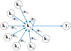
Figure 1: The aggregation process of graph attention.

The feature selection scheme can effectively eliminate some abnormal samples, but the relationship between the samples is not analyzed. Sample reweighting based methods aljundi2015landmarks  long2014transfer  hubert2016learning can solve the problem effectively. These methods performed knowledge transfer using landmarks, i.e., the most relevant samples, which is optimal than using all the samples. However, these methods assume that the landmarks of samples are the same, i.e., the set of the most relevant samples is uniform with respect to each sample. However, the assumption ignores the hierarchy of samples. Motivated by the advantage of attention mechanism velickovic2017graph , we introduce a graph-attentional mechanism based landmark selection, whose idea is to represent each point in the graph by its neighbors using attention coefficient matrix. Through assigning arbitrary weights to neighbors, it can be applied to graph nodes with varying degrees. In order to obtain features with sufficient expression, a shared transformation matrix $\mathbf{P}$ is applied to each sample . We use cosine similarity to compute the attentional coefficient matrix $\mathbf{A}$ as follows:

$$[\mathbf{A}]_{ij}=\begin{cases}\frac{(\mathbf{P}^{\top}\mathbf{k}_{i})^{\top}\mathbf{P}^{\top}\mathbf{k}_{j}}{\|\mathbf{P}^{\top}\mathbf{k}_{i}\|_{2}\|\mathbf{P}^{\top}\mathbf{k}_{j}\|_{2}},&\text{if $\mathbf{P}^{\top}\mathbf{k}_{i}\in\mathcal{N}_{k}(\mathbf{P}^{\top}\mathbf{k}_{j})$ }\\ 0,&\text{otherwise}\end{cases}$$ (24)

which indicates the importance of feature of sample $i$ to sample $j$, where $\mathcal{N}_{k}(\textbf{{X}})$ represents the set of $k$ nearest neighbors of X. During the optimization, we normalize them across all choices of $j$:

$$[\mathbf{B}]_{ij}=\frac{[\mathbf{A}]_{ij}}{\sum_{k\in\mathcal{N}_{j}}[\mathbf{A}]_{kj}}$$ (25)

We then use $\mathbf{B}$ to calculate a linear combination of the features corresponding to them, and the final output features of each sample can be represented by:

$$\mathbf{y}_{j}=\sum_{i\in\mathcal{N}_{j}}\mathbf{P}^{\top}\mathbf{k}_{i}(\mathbf{B})_{i,j}=\mathbf{P}^{\top}\mathbf{K}\mathbf{b}_{j}$$ (26)

where $\mathbf{b}_{j}$ represents the $j$th column of $\mathbf{B}$. The aggregation process of the graph-attentional mechanism is illustrated in Figure 1. Feature selection and landmark selection analyze the features of the samples from different aspects. The former eliminates some abnormal samples that are not conducive to adaptation, which is analyzed from the perspective of global samples, and the latter represents each sample by its neighbors, which is analyzed from the perspective of local samples. The combination of the two schemes can effectively promote domain adaptation.

We add graph-attentional landmark selection to the model (3.4.3),and the final model is as follows:

$$\min_{\mathbf{P}} ~{}tr(\mathbf{P}^{\top}\mathbf{K}\mathbf{B}(\mathbf{M}+\beta\mathbf{L})\mathbf{B}^{\top}\mathbf{K}\mathbf{P})+\gamma\|(\textbf{{H}}-\mathbf{P}^{\top}\mathbf{K}\mathbf{B})\mathbf{R}\|_{F}^{2}$$

$$+\lambda_{1}\|\mathbf{P}\|_{2,1}+\lambda_{2}tr(\mathbf{P}^{\top}\mathbf{K}\mathbf{P})$$ (27)

where $\lambda_{1}$ and $\lambda_{2}$ are the regularization parameters, $\mathbf{R}\in\mathbb{R}^{N\times N}$ is a diagonal domain indicator matrix with $\mathbf{R}_{ii}=1$ if $i$ belongs to source domain, otherwise $\mathbf{R}_{ii}=0$, H is the ground truth label matrix of samples from source and target domains, where the labels of samples from target domain can be filtered out by the diagonal matrix $\mathbf{R}$.

3.6 Optimization

For the optimization problem (3.5), we take the derivative with respect to $\mathbf{P}$, set the derivative to zero, and obtain:

$$\mathbf{P}=\gamma(\mathbf{KB}\mathbf{U}\mathbf{B}^{\top}\mathbf{K}+\lambda_{1}\mathbf{F}+\lambda_{2}\mathbf{K})^{-1}\mathbf{KBR}\textbf{{H}}^{\top}$$ (28)

where $\mathbf{U}=\mathbf{M}+\beta\mathbf{L}+\gamma\mathbf{R}$. Note that $\|\mathbf{P}\|_{2,1}$ is not smooth, so we compute its subgradient $\mathbf{F}$ gu2011joint  li2016joint as follows:

$$\mathbf{F}_{i,i}=\begin{cases}0,&\text{if $\mathbf{p}^{i}=\mathbf{0}$}\\ \frac{1}{2\|\mathbf{p}^{i}\|_{2}},&\text{otherwise}\end{cases}$$ (29)

where $\mathbf{p}^{i}$ denotes the $i$th row of $\mathbf{P}$. Then, we compute $\mathbf{B}$ via Eq. (24)(25). We show an algorithm of solving (3.5) in Algorithm 1, and give algorithm for testing in Algorithm 2.

Algorithm 1 Optimization of Eq. (3.5)

1:Data $\textbf{{X}}=[\textbf{{X}}_{s},\textbf{{X}}_{t}]$; label matrix $\textbf{{H}}_{s}$; manifold feature dimension $d$; parameters $\beta,\gamma,\lambda_{1},\lambda_{2}$;

2:Transformation matrix $\mathbf{P}$, attention coefficient matrix $\mathbf{B}$;

3:Initialize $\mathbf{A}=\mathbf{I}$, $\mathbf{F}=\mathbf{I}$;

4:Compute $\mathbf{B}$ via Eq. (25);

5:Learn manifold feature transformation kernel $\mathbf{Q}$ via Eq. (20), and compute manifold feature ${\mathbf{Z}}=\mathbf{Q}^{\frac{1}{2}}\textbf{{X}}$;

6:Compute kernel matrix $\mathbf{K}=\Psi(\mathbf{Z},\mathbf{Z})$ via Eq. (21);

7:Obtain the pseudo labels of $\mathbf{K}_{t}$ via classifier trained by $\mathbf{K}_{s}$;

8:while not converge or reach maximum iterations do

9:     Compute $\mathbf{M}$ via Eq. (6)(13);

10:     Compute $\mu$ via Eq. (14);

11:     Compute $\mathbf{P}$ via Eq. (28);

12:     Compute $\mathbf{F}$ via Eq. (29);

13:     Compute $\mathbf{B}$ via Eq. (24)(25);

14:     Compute the pseudo labels of $\mathbf{Y}_{t}$ via classifier trained by $\mathbf{Y}_{s}$;

15:end while

Algorithm 2 Testing of GGLS

1:Data $\textbf{{X}}_{t}$; manifold feature $\mathbf{Z}_{s}$;manifold feature transformation kernel $\mathbf{Q}$; Transformation matrix $\mathbf{P}$, attention coefficient matrix $\mathbf{B}$;

2:Labels of $\mathbf{Y}_{t}$;

3:Compute manifold feature ${\mathbf{Z}_{t}}=\mathbf{Q}^{\frac{1}{2}}\textbf{{X}}_{t}$;

4:Compute kernel matrix $\mathbf{K}=\Psi([\mathbf{Z}_{s},\mathbf{Z}_{t}],[\mathbf{Z}_{s},\mathbf{Z}_{t}])$ via Eq. (21);

5:Compute output feature $\mathbf{Y}_{t}=\mathbf{P}^{\top}\mathbf{K}\mathbf{B}_{N_{s}+1:N}$;

6:Compute the labels of $\mathbf{Y}_{t}$ via classifier trained by $\mathbf{Y}_{s}$;

4 Analysis

4.1 Theory Analysis

In general, our final model is presented in the coarse-to-fine form. We first propose a coarse model (3.3.3) by analysis as a whole, and then optimize the model for some specific problems to further improve the model performance. To minimize the difference of distribution between the source domain and target domain, our coarse model (3.3.3) analyzes global, local, and individual characteristics of sample data. According to the three characteristics, we respectively propose distribution adaptation term (the first term of model (3.3.3), a locality preservation term (the second term of model (3.3.3), and a discrimination preservation term (the third term of model 3.3.3). The three terms can balance the contributions of marginal and conditional distributions based on all the samples, preserve the local topology structure of samples from source and target domains, and preserve the discriminative power of samples from the source domain, respectively. To better exploit the three characteristics of model 3.3.3), we analyze it from three aspects. First, We transform the sample features in the original space into manifolds, which can avoid feature distortion. Secondly, we propose feature selection scheme to handle these abnormal samples. Thirdly, we analyze the relationship between the samples by landmark selection. In fact, these three aspects are mainly discussed from the three perspectives of feature space, feature selection and the relationship between features. It can be seen from the subsequent experiments that our model has significantly improved after further improvement.

4.2 Complexity Analysis

The computational costs of Algorithm 1 consists of five major parts: computing $\mathbf{B}$ via solving Eq. (25), computing $\mathbf{K}$ via Eq. (21), computing $\mathbf{M}$ via Eq. (6)(13), computing $\mathbf{P}$ via Eq. (28), and computing $\mathbf{F}$ via Eq. (29). The computational complexity can be seen in Table 1. The computation of $\mathbf{B}$ costs $\mathcal{O}$($N^{2}$), the computation of $\mathbf{K}$ costs $\mathcal{O}$($N^{2}$), the computation of $\mathbf{M}$ costs $\mathcal{O}$($N^{2}$), the computation of $\mathbf{P}$ costs $\mathcal{O}$($N^{2}$), the computation of $\mathbf{F}$ costs $\mathcal{O}$($N^{2}$). Suppose the Algorithm 1 will converge after $T$ iterations, the overall computational cost of Algorithm 1 is $\mathcal{O}(5TN^{2})$.

Table 1: Phase-wise computational complexity.

Phase	Line num of Algorithm 1	Complexity
Computation of $\mathbf{B}$	line 2	$\mathcal{O}$($N^{2}$)
Computation of $\mathbf{K}$	line 4	$\mathcal{O}$($N^{2}$)
Computation of $\mathbf{M}$	line 8	$\mathcal{O}$($N^{2}$)
Computation of $\mathbf{P}$	line 9	$\mathcal{O}$($N^{2}$)
Computation of $\mathbf{F}$	line 10	$\mathcal{O}$($N^{2}$)

4.3 Convergence Analysis

Algorithm 1 solves problem (3.5) with locally optimal solution of $\mathbf{P}$. In order to demonstrate this convergence, Lemma 3 is utilized subsequently, which is proposed and proven in nie2010efficient .

Lemma 3: For any nonzero vectors $\mathbf{u},\mathbf{v}\in\mathbb{R}^{c}$, it holds that

$$\|\mathbf{u}\|_{2}-\frac{\|\mathbf{u}\|_{2}^{2}}{2\|\mathbf{v}\|_{2}}\leq\|\mathbf{v}\|_{2}-\frac{\|\mathbf{v}\|_{2}^{2}}{2\|\mathbf{v}\|_{2}}$$ (30)

Theorem 1: Algorithm 1 decreases problem (3.5) by iteratively updating $\mathbf{P}$ with its optimal solution until convergence.

Proof: Denote the objective value in the $t$th iteration of problem (3.5) as $\emph{f}(\mathbf{P}_{(t)})$, i.e.,

$$\emph{f}(\mathbf{P}_{(t)})=tr(\mathbf{P}_{(t)}^{\top}\mathbf{\Gamma}\mathbf{P}_{(t)})+\gamma\|(\textbf{{H}}-\mathbf{P}_{(t)}^{\top}\mathbf{K}\mathbf{B})\mathbf{R}\|_{F}^{2}$$ (31)

where $\mathbf{\Gamma}=\mathbf{K}\mathbf{B}(\mathbf{M}+\beta\mathbf{L})\mathbf{B}^{\top}\mathbf{K}+\lambda_{1}\mathbf{F}+\lambda_{2}\mathbf{K}$.

Since Algorithm 1 updates $\mathbf{P}$ with the optimal solution in each iteration, for the $(t+1)$th iteration, it must hold

$$\emph{f}(\mathbf{P}_{(t+1)})\leq\emph{f}(\mathbf{P}_{(t)})$$ (32)

and

$$\emph{f}(\mathbf{P}_{(t+1)})+\lambda_{1}\sum_{i=1}^{N}\frac{\|\mathbf{p}_{(t+1)}^{i}\|^{2}}{2\|\mathbf{p}_{(t)}^{i}\|}\leq\emph{f}(\mathbf{P}_{(t)})+\lambda_{1}\sum_{i=1}^{N}\frac{\|\mathbf{p}_{(t)}^{i}\|^{2}}{2\|\mathbf{p}_{(t)}^{i}\|}$$ (33)

According to Lemma 3, we have

$$\begin{array}[]{l}{\|\mathbf{p}_{(t+1)}^{i}\|_{2}-\frac{\|\mathbf{p}_{(t+1)}^{i}\|_{2}^{2}}{2\|\mathbf{p}_{(t)}^{i}\|_{2}}}{\quad\leq\|\mathbf{p}_{(t)}^{i}\|_{2}-\frac{\|\mathbf{p}_{(t)}^{i}\|_{2}^{2}}{2\|\mathbf{p}_{(t)}^{i}\|_{2}}}\\ {\Rightarrow\lambda_{1}\sum_{i=1}^{N}\|\mathbf{p}_{(t+1)}^{i}\|_{2}-\lambda_{1}\sum_{i=1}^{N}\frac{\|\mathbf{p}_{(t+1)}^{i}\|_{2}^{2}}{2\|\mathbf{p}_{(t)}^{i}\|_{2}}}\\ {\quad\leq\lambda_{1}\sum_{i=1}^{N}\|\mathbf{p}_{(t)}^{i}\|_{2}-\lambda_{1}\sum_{i=1}^{N}\frac{\|\mathbf{p}_{(t)}^{i}\|_{2}^{2}}{2\|\mathbf{p}_{(t)}^{i}\|_{2}}}\end{array}$$ (37)

Then, adding (37) to (33), we have

$$\emph{f}(\mathbf{P}_{(t+1)})+\lambda_{1}\sum_{i=1}^{N}\frac{\|\mathbf{p}_{(t+1)}^{i}\|^{2}}{2\|\mathbf{p}_{(t)}^{i}\|}+\lambda_{1}\sum_{i=1}^{N}(\|\mathbf{p}_{(t+1)}^{i}\|_{2}-\frac{\|\mathbf{p}_{(t+1)}^{i}\|_{2}^{2}}{2\|\mathbf{p}_{(t)}^{i}\|_{2}})$$

$$\leq\emph{f}(\mathbf{P}_{(t)})+\lambda_{1}\sum_{i=1}^{N}\frac{\|\mathbf{p}_{(t)}^{i}\|^{2}}{2\|\mathbf{p}_{(t)}^{i}\|}+\lambda_{1}\sum_{i=1}^{N}(\|\mathbf{p}_{(t)}^{i}\|_{2}-\frac{\|\mathbf{p}_{(t)}^{i}\|_{2}^{2}}{2\|\mathbf{p}_{(t)}^{i}\|_{2}})$$ (38)

Thus, we have

$$\emph{f}(\mathbf{P}_{(t+1)})+\lambda_{1}\sum_{i=1}^{N}(\|\mathbf{p}_{(t+1)}^{i}\|_{2})\leq\emph{f}(\mathbf{P}_{(t)})+\lambda_{1}\sum_{i=1}^{N}(\|\mathbf{p}_{(t)}^{i}\|_{2})$$

$$\Rightarrow\emph{f}(\mathbf{P}_{(t+1)})+\lambda_{1}\|\mathbf{P}_{(t+1)}\|_{2,1}\leq\emph{f}(\mathbf{P}_{(t)})+\lambda_{1}\|\mathbf{P}_{(t)}\|_{2,1}$$ (39)

which completes the proof.

5 Experiments

In this section, we evaluate GGLS on eight publicly available datasets, and compare with some state-of-the-art methods including traditional domain adaptation methods and depth domain adaptation methods, and also introduce the parameters analysis and ablation study in this section.

5.1 Experimental Settings

Office+Caltech object datasets gong2012geodesic consists of four datasets: Amazon(A), DSLR(D), Webcam(W), and Caltech-256(C) (4 datasets domain adaptation, 4DA). The first three datasets Saenko2010Adapting contains 31 classes, and the last dataset griffin2007caltech contains 256 classes. There are 10 common classes shared by the four datasets. Furthermore, we consider two types of features: SURF features of 800 dimensions, and Decaf₆ features of 4096 dimensions donahue2014decaf , which are the activations of the 6th fully connected layer of a convolutional network trained on imageNet. We follow the setting of zhang2017joint to construct 12 cross-domain datasets, which are listed in Tables 2, 3, where C$\rightarrow$A represents C is source domain and A is target domain. For the parameters, we set $\beta=0.1$, $\gamma=0.1$, $\lambda_{1}=0.001$, $\lambda_{1}=0.01$, $T=10$, $d=30$, and $k=3,9$ for SURF and Decaf₆ features.

USPS (U) lecun1998gradient and MNIST (M) hull1994database are digit datasets containing handwritten digits from 0-9. There are 10 common classes shared by the two datasets. MNIST dataset contains 60,000 training samples and 10,000 testing samples of size $28\times 28$. USPS dataset contains 7,291 training samples and 2,007 testing samples of size $16\times 16$. For fair comparison, we extract SURF features of 256 dimensions. We construct two cross-domain datasets: U$\rightarrow$M and M$\rightarrow$U. For the parameters, we set $\beta=0.1$, $\gamma=0.1$, $\lambda_{1}=0.0001$, $\lambda_{1}=0.01$, $T=10$, $d=30$, and $k=3$.

ImageNet (I) and VOC2007 (V) are large-scale image datasets. We follow the fang2013unbiased to select five common classes shared by the two datasets: bird, cat, chair, dog and person. We extract Decaf₆ features of 4096 dimensions and construct two cross-domain datasets: I$\rightarrow$V and V$\rightarrow$I. For the parameters, we set $\beta=0.1$, $\gamma=0.1$, $\lambda_{1}=0.001$, $\lambda_{1}=0.01$, $T=10$, $d=20$, and $k=5$.

CIFAR10(CI) and STL10(S) are both 10 class datasets. CIFAR10 contains 50,000 training samples of size $32\times 32$, while STL10 contains 5,000 training samples of size $96\times 96$. There are 9 overlapping classes between these two datasets. Following roy2019unsupervised we remove non-overlapping classes - “frog” and “monkey” from these two datasets. We use ResNet50 to extract features and construct two cross-domain datasets: CI$\rightarrow$S and S$\rightarrow$CI. For the parameters, we set $\beta=0.1$, $\gamma=0.1$, $\lambda_{1}=0.001$, $\lambda_{1}=0.01$, $T=10$, $d=20$, and $k=5$.

Eight publicly available datasets are shown in Fig. 2, including Office+Caltech object datasets, which consists of four datasets: Amazon(A), DSLR(D), Webcam(W), and Caltech-256(C), USPS(U), MNIST(M), ImageNet(I) and VOC2007(V).

Figure 2: Some selected samples from Office+Caltech, USPS, MNIST, ImageNet and VOC2007.

In this section, the classification accuracy of the target domain is used as the evaluation index, which has been widely applied in the existing methods, namely:

$$Accuracy=\frac{|{{\bf{x}}:{\bf{x}}\in{{\bf{X}}_{t}}\wedge{{\widehat{\bf{l}}}_{t}}={{\bf{l}}_{t}}}|}{|{{\bf{x}}:{\bf{x}}\in{{\bf{X}}_{t}}}|}$$ (40)

5.2 Results

In this section, the comparison methods include traditional domain adaptation methods and depth domain adaptation methods.

Traditional domain adaptation methods:

1. $\mathbf{kNN}$(k=1) and $\mathbf{PCA}$

2. $\mathbf{GFK}$(Geodesic Flow Kernel) gong2012geodesic :performs manifold feature learning

3. $\mathbf{TCA}$(Transfer Component Analysis) pan2010domain : performs marginal distribution adaptation

4. $\mathbf{JDA}$(Joint Distribution Alignment) long2013transfer : performs marginal and conditional distribution adaptation

5. $\mathbf{SA}$(Subspace Alignment) fernando2013unsupervised : performs subspace alignment

6. $\mathbf{\mathbf{TJM}}$(Transfer Joint Matching) long2014transfer :performs marginal distribution adaptation with sample selection of source domain

7. $\mathbf{MLS}$(Multiscale Landmarks Selection) aljundi2015landmarks : performs landmark selection on both domains

8. $\mathbf{\mathbf{SCA}}$(Scatter Component Analysis) ghifary2017scatter : performs scatter adaptation in subspace

9. $\mathbf{JGSA}$(Joint Geometrical and Statistical Alignment) zhang2017joint :performs marginal and conditional distribution adaptation with label information

10. $\mathbf{TIT}$(Transfer Independently Together) li2018transfer : performs landmark selection based on graph optimization

11. $\mathbf{MEDA}$(Manifold Embedded Distribution Alignment) wang2018visual : performs distribution alignment based on structural risk minimization

12. $\mathbf{CAPLS}$( Confidence-Aware Pseudo Label Selection) wang2019unifying : performs confidence-aware pseudo label selection scheme

13. $\mathbf{SPL}$( Selective Pseudo-Labeling) wang2020unsupervised : performs selective pseudo-labeling strategy based on structured prediction

Deep domain adaptation approaches:

1. $\mathbf{AlexNet}$ krizhevsky2012imagenet

2. $\mathbf{DDC}$(Deep Domain Confusion) tzeng2014deep :performs single-layer deep adaptation with MMD loss

3. $\mathbf{DAN}$(Deep Adaptation Network) long2014domain performs multi-layer adaptation with multiple kernel MMD

4. $\mathbf{DCORAL}$(Deep CORAL) sun2016deep :performs neural network with CORAL loss

5. $\mathbf{DUCDA}$(Deep Unsupervised Convolutional Domain Adaptation) zhuo2017deep : performs adaptation with attention and CORAL loss

6. $\mathbf{ReverseGrad}$(Reverse Gradient) ganin2015unsupervised : performs gradient reversal layer

7. $\mathbf{DRCN}$(Deep Reconstruction Classification Network ) ghifary2016deep : performs shared encoding representation for alternately learning (source) label prediction and (target) data reconstruction

8. $\mathbf{AutoDIAL}$(Automatic DomaIn Alignment Layers) maria2017autodial : performs domain alignment layers

9. $\mathbf{DWT}$(Domain-specific Whitening Transform) roy2019unsupervised : performs domain specific feature whitening

Table 2: Accuracy results (%) on Office+Caltech10 datasets using SURF features.

Data	1NN	PCA	GFK	TCA	JDA	TJM	SCA	MLS	JGSA	TIT	MEDA	GGLS
C$\rightarrow$ A	23.7	39.5	46.0	45.6	43.1	46.8	45.6	53.6	53.1	59.7	56.5	$\mathbf{58.2}$
C$\rightarrow$ W	25.8	34.6	37.0	39.3	39.3	39.0	40.0	44.1	48.5	51.5	53.9	$\mathbf{55.3}$
C$\rightarrow$ D	25.5	44.6	40.8	45.9	49.0	44.6	47.1	45.2	48.4	48.4	50.3	$\mathbf{51.6}$
A$\rightarrow$ C	26.0	39.0	40.7	42.0	40.9	39.5	39.7	45.0	41.5	47.5	43.9	$\mathbf{48.6}$
A$\rightarrow$ W	29.8	35.9	37.0	40.0	38.0	42.0	34.9	41.1	45.1	45.4	$\mathbf{53.2}$	51.2
A$\rightarrow$ D	25.5	33.8	40.1	35.7	42.0	45.2	39.5	39.5	45.2	47.1	45.9	$\mathbf{51.0}$
W$\rightarrow$ C	19.9	28.2	24.8	31.5	33.0	30.2	31.1	31.6	33.6	$\mathbf{34.9}$	34.0	32.6
W$\rightarrow$ A	23.0	29.1	27.6	30.5	29.8	30.0	30.0	35.9	40.8	40.2	$\mathbf{42.7}$	40.7
W$\rightarrow$ D	59.2	89.2	85.4	91.1	$\mathbf{92.4}$	89.2	87.3	84.7	88.5	87.9	88.5	90.4
D$\rightarrow$ C	26.3	29.7	29.3	33.0	31.2	31.4	30.7	39.2	30.3	$\mathbf{36.7}$	34.9	35.2
D$\rightarrow$ A	28.5	33.2	28.7	32.8	33.4	32.8	31.6	34.6	38.7	42.1	41.2	$\mathbf{44.3}$
D$\rightarrow$ W	63.4	86.1	80.3	87.5	89.2	85.4	84.4	82.4	$\mathbf{93.2}$	84.8	87.5	90.2
Average	31.4	43.6	43.1	46.2	46.8	46.3	45.2	48.1	50.6	52.2	52.7	$\mathbf{54.1}$

Table 3: Comprisons with traditional methods on Office+Caltech10 datasets using DeCaf₆ features.

Data	1NN	PCA	GFK	TCA	JDA	TJM	SCA	JGSA	CAPLS	MEDA	SPL	GGLS
C$\rightarrow$ A	87.3	88.1	88.2	89.8	89.6	88.8	89.5	91.1	90.8	92.3	92.7	$\mathbf{94.9}$
C$\rightarrow$ W	72.5	83.4	77.6	78.3	85.1	81.4	85.4	86.8	85.4	91.2	93.2	$\mathbf{93.6}$
C$\rightarrow$ D	79.6	84.1	86.6	85.4	89.8	84.7	87.9	93.6	$\mathbf{95.5}$	89.8	98.7	94.9
A$\rightarrow$ C	71.7	79.3	79.2	82.6	83.6	84.3	78.8	84.9	86.1	89.2	87.4	$\mathbf{89.7}$
A$\rightarrow$ W	68.1	70.9	70.9	74.2	78.3	71.9	75.9	81.0	87.1	$\mathbf{90.8}$	95.3	87.1
A$\rightarrow$ D	74.5	82.2	82.2	81.5	80.3	76.4	85.4	88.5	$\mathbf{94.9}$	87.9	89.2	88.5
W$\rightarrow$ C	55.3	70.3	69.8	80.4	84.8	83.0	74.8	85.0	88.2	88.7	87.0	$\mathbf{89.9}$
W$\rightarrow$ A	62.6	73.5	76.8	84.1	90.3	87.6	86.1	90.7	92.3	92.5	92.0	$\mathbf{94.2}$
W$\rightarrow$ D	98.1	99.4	$\mathbf{100}$	$\mathbf{100}$	$\mathbf{100}$	$\mathbf{100}$	$\mathbf{100}$	$\mathbf{100}$	$\mathbf{100}$	99.4	$\mathbf{100}$	$\mathbf{100}$
D$\rightarrow$ C	42.1	71.7	71.4	82.3	85.5	83.8	78.1	86.2	88.8	88.2	88.6	$\mathbf{90.2}$
D$\rightarrow$ A	50.0	79.2	76.3	89.1	91.7	90.3	90.0	92.0	93.0	92.6	92.9	$\mathbf{94.1}$
D$\rightarrow$ W	91.5	98.0	99.3	99.7	99.7	99.3	98.6	99.7	$\mathbf{100}$	98.6	98.6	$\mathbf{100}$
Average	71.1	81.7	81.5	85.6	88.2	86.0	85.9	90.0	91.8	91.8	93.0	$\mathbf{93.1}$

Table 4: Comprisons with deep learning based methods on Office+Caltech10 datasets using DeCaf6 features.

Data	AlexNet	DDC	DAN	DCORAL	DUCDA	GGLS
C$\rightarrow$ A	91.9	91.9	92.0	92.4	92.8	$\mathbf{94.9}$
C$\rightarrow$ W	83.7	85.4	90.6	91.1	91.6	$\mathbf{93.6}$
C$\rightarrow$ D	87.1	88.8	89.3	91.4	91.7	$\mathbf{94.9}$
A$\rightarrow$ C	83.0	85.0	84.1	84.7	84.8	$\mathbf{89.7}$
A$\rightarrow$ W	79.5	86.1	$\mathbf{91.8}$	$-$	$-$	87.1
A$\rightarrow$ D	87.4	89.0	$\mathbf{91.7}$	$-$	$-$	$88.5$
W$\rightarrow$ C	73.0	78.0	81.2	79.3	80.2	$\mathbf{89.9}$
W$\rightarrow$ A	83.8	84.9	92.1	$-$	$-$	$\mathbf{94.2}$
W$\rightarrow$ D	$\mathbf{100}$	$\mathbf{100}$	$\mathbf{100}$	$-$	$-$	$\mathbf{100}$
D$\rightarrow$ C	79.0	81.1	80.3	82.8	82.5	$\mathbf{90.2}$
D$\rightarrow$ A	87.1	89.5	90.0	$-$	$-$	$\mathbf{94.1}$
D$\rightarrow$ W	97.7	98.2	98.5	$-$	$-$	$\mathbf{100}$
Average	86.1	88.2	90.1	$-$	$-$	$\mathbf{93.1}$

Table 5: Accuracy results(%) on USPS+MNIST and ImageNet+VOC2007 datasets.

Data	1NN	PCA	GFK	TCA	JDA	TJM	SCA	JGSA	MEDA	GGLS
U$\rightarrow$ M	44.7	45.0	46.5	51.2	59.7	52.3	48.0	68.2	72.1	$\mathbf{74.7}$
M$\rightarrow$ U	65.9	66.2	61.2	56.3	67.3	63.3	65.1	80.4	89.5	$\mathbf{90.6}$
I$\rightarrow$ V	50.8	58.4	59.5	63.7	63.4	63.7	$-$	52.3	67.3	$\mathbf{68.1}$
V$\rightarrow$ I	38.2	65.1	73.8	64.9	70.2	73.0	$-$	70.6	74.7	$\mathbf{78.3}$
Average	49.9	58.7	60.2	59.0	65.1	63.1	$-$	67.9	75.9	$\mathbf{77.9}$

Table 6: Accuracy results(%) on CIFAR10 and STL10 datasets.

Data	SA	ReverseGrad	DRCN	AutoDIAL	DWT	GGLS
CI$\rightarrow$ S	62.9	66.1	66.4	79.1	79.7	$\mathbf{80.1}$
S$\rightarrow$ CI	54.0	56.9	58.9	70.2	$\mathbf{71.2}$	70.6
Average	58.5	61.5	62.7	74.6	$\mathbf{75.5}$	75.4

Table 7: Results of Wilcoxon rank sum tests for GGLS

Results of Tables2 based		Results of Tables 3 and  4 based		Results of Tables 5 based		Results of Tables 6 based
GGLS vs.	p-values	GGLS vs.	p-values	GGLS vs.	p-values	GGLS vs.	p-values
1NN	0.003	1NN	0.001	1NN	0.009	SA	0.121
PCA	0.024	PCA	0.003	PCA	0.009	ReverseGrad	0.121
GFK	0.035	GFK	0.004	GFK	0.016	DRCN	0.121
TCA	0.073	TCA	0.008	TCA	0.009	AutoDIAL	0.439
JDA	0.083	JDA	0.038	JDA	0.016	DWT	1.000
TJM	0.065	TJM	0.013	TJM	0.016
SCA	0.033	SCA	0.011	JGSA	0.175
MLS	0.184	JGSA	0.094	MEDA	0.403
JGSA	0.326	CAPLS	0.470
TIT	0.525	MEDA	0.299
MEDA	0.686	SPL	0.729
		AlexNet	0.011
		DDC	0.021
		DAN	0.248

Tables 2, 3, 4, 5 and 6 show the accuracy results on the different datasets. From Tables 2, 3 and 5, it can be observed that transfer learning methods outperform 1NN and PCA, which indicates transfer learning is valuable and practical in real world applications for classification. GGLS outperforms the state-of-the-art methods in 19 out of 28 cases, and the average accuracy is 74.2%. Besides, GGLS achieves the best accuracy in 24 out of 28 cases compared with the baseline method MEDA. These results indicate that GGLS can deal with distribution divergence better. Since these datasets have a large differences, it demonstrates that GGLS has strong generalization ability and robustness in domain adaptation. From Table 4 and 6, we can see that GGLS also outperforms most of the deep learning based methods, and only worse than DWT, which use deep learning technology to construct domain-specific alignment layers. This layer projects the source domain and target domain into a common spherical distribution. However, DWT often tunes a lot of hyperparameters before obtaining the optimal results. Compared with DWT, GGLS has a more simple architecture and fewer parameters, which can be set easily. Therefore, GGLS has high accuracy and efficiency. Furthermore, we pay attention to the performance of MLS, TJM, and GGLS, which use samples reweighting. We find that GGLS outperforms the other three methods in many cases. It indicates that it is better to select the landmarks of different samples independently, rather than simply select the same landmarks of samples. GFK and MEDA learn feature in the manifold, and JGSA preserves discriminative information from the source domain, yet none of them outperforms GGLS in average. It exactly demonstrates that GGLS with optimizing them together is more optimal than optimizing them separately. MEDA learns feature in manifold and preserves discriminative information from the source domain, but it does not consider the samples reweighting. As a result, its performance is worse than GGLS. Compared with TIT, which also combine sample reweighting and feature matching, GGLS has better performance. This shows that our combination method is more effective.

Based on the results of Tables 2, 3, 4, 5 and 6 , we further conduct a Wilcoxon rank sum statistic for GGLS with other methods shown in Table 7. The Wilcoxon rank sum test tests the null hypothesis that two sets of measurements are drawn from the same distribution. The alternative hypothesis is that values in one sample are more likely to be larger than the values in the other sample. The p-value denotes the probability of observing the given result by chance if the null hypothesis is true. Small values of p cast doubt on the validity of the null hypothesis. That is to say, the greater the value of p is, the smaller the significant difference between the two classes is; and vice versa. As we can see from Table 7, there are significantly difference (p-value below 0.1) between GGLS and many compared methods. In other words, GGLS is significantly better than these methods. For other methods like JSGA, TIT, MEDA, CAPLS, although the difference is not significant, the p-value is also small. From the results of Tables 6 based in Table 7, we can observe that the p-value of GGLS and DWT is 1.000, which further demonstrated that our method is comparable to DWT.

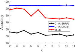
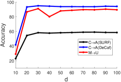
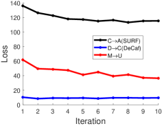
Figure 3: Domain adaptation results. (a) shows the results of different neighbor numbers; (b) shows the results of different subspace dimension. (c) shows the convergence curves.

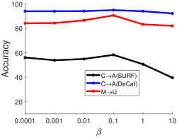
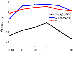
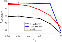
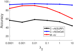
Figure 4: Accuracy w.r.t different $\beta$, $\gamma$, $\lambda_{1}$, $\lambda_{2}$, respectively.

5.3 Parameter Analysis

We show further details for parameter selection including the number of neighbors $k$, subspace dimension $d$, iteration number $T$, and other regularization parameters $\beta,\gamma,\lambda_{1},\lambda_{2}$. Fig. 3-3 show the effects of $k$, $d$ and $T$, respectively. We can observe that GGLS reaches the better performance when $k$ takes $3,9,3$ for $\text{C}\rightarrow A$(SURF), $C\rightarrow A$(DeCaf) and $M\rightarrow U$, respectively, and shows a high robustness for $d$ from $[20,100]$. For the number of iteration $T$, the results can be converged to the optimum value after a few iterations. Therefore, we set $T=10$. Fig. 4-4 show the effects of regularization parameters $\beta$, $\gamma$, $\lambda_{1}$, $\lambda_{2}$, respectively. We find that GGLS can achieve a robust performance in a wide range of parameter values, whose optimal ranges are $\beta\in[0.0001,1]$, $\gamma\in[0.001,1]$, $\lambda_{1}\in[0.0001,0.1]$ and $\lambda_{2}\in[0.0001,1]$, respectively. When these values of parameters are too large, the learned transformation matrix may be overfitting and thus the performance degrades.

5.4 Ablation Study

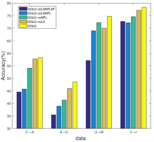
Figure 5: Evaluation of landmark selection and manifold feature learning.

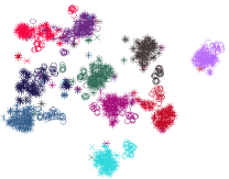
(a) Decaf

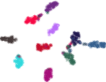
(b) GGLS-noLS

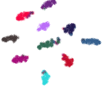
(c) GGLS

Figure 6: A t-SNE visualization of feature representations of different methods. Asterisk represents the features of Amazon(A), and circle represents the features of Webcam(W), where different colors represent different classes.

To verify the effectiveness of our landmark selection and manifold feature learning, we compare the experimental results of GGLS with and without landmark selection and manifold feature learning as shown in Fig.5, where GGLS-noLS represents GGLS without landmark selection, GGLS-noMFL represents GGLS without manifold feature learning, and GGLS-noLSMFL represents GGLS without landmark selection and manifold feature learning. The results clearly indicate that our proposed landmark selection and manifold feature learning are all important and effective for transfer learning. GGLS-noLSMFL also can achieve comparable performance, but GGLS with landmark selection and manifold feature learning would reach better accuracies. We further verify the effectiveness of kernel function by comparing GGLS-noLSMFL and GGLS-noLSMFLKF, where GGLS-noLSMFLKF represents GGLS-noLSMFL without kernel function. From Fig.5 we can observe that GGLS-noLSMFL achieves better performance than GGLS-noLSMFLKF. This indicates that it is more effective to explore the distribution of source domain and target domain in kernel space.

The parameter $\mu$ balances the contributions of marginal distribution and conditional distribution. In order to evaluate the effectiveness of calculated $\mu$ by Eq. (14), we compare our solution with $\mu=0.5$, which means the contribution of marginal distribution and conditional distribution are the same. The comparison is shown in Table8, where the improvement shows the performance variation. For example, the improvement of mean accuracy on M$\rightarrow$ U is: $(90.6-89.2)/89.2\times 100\%=1.6\%$. From the table, we can see that the performance of our solution is better than $\mu=0.5$, which demonstrates the effectiveness in calculating $\mu$. Therefore, the importance of the two distributions is significantly different, which explains that the improvement is necessary.

Data	$\mu$=0.5	Estimated $\mu$	Improvement
A$\rightarrow$ C	48.5	48.6	0.2%
A$\rightarrow$ D	49.7	51.0	2.6%
C$\rightarrow$ A(Decaf6)	94.3	94.9	0.6%
D$\rightarrow$ A(Decaf6)	93.6	94.1	0.5%
M$\rightarrow$ U	89.2	90.6	1.6%
V$\rightarrow$ I	77.5	78.3	1.0%

Table 8: Comparison of $\mu$=0.5 and our estimated $\mu$.

5.5 Visualization

The feature representations of different methods can be investigated qualitatively. Therefore, we use t-SNE to visualize high-dimensional data by giving each datapoint a location in the projected 2D space. Fig. 6 shows the visualization of feature representations of task A$\rightarrow$W by different methods, where GGLS-noLS represents GGLS without landmark selection. It can be seen that the source and target are not aligned well with the Decaf feature, the samples from different classes are confused, and the inter-class distance is also small, which can easily lead to misclassification. They are aligned better and categories are discriminated better by GGLS-noLS, while GGLS is evidently better than GGLS-noLS. From Fig. 6(c) we can see that the intra-class samples are more compact and the distributions between different classes are more dispersed. That is to say, GGLS can further reduce the distance of intra-class and increase the distance of inter-classes. This shows the benefit of landmark selection.

6 Conclusion

In this paper, we propose a Grassmannian graph-attentional landmark selection (GGLS) framework for visual domain adaptation, which considers sample reweighting and feature matching simultaneously. GGLS learns an attention mechanism based sample reweighting, which treats the landmarks of each sample differently, and performs distribution adaptation and knowledge adaptation over the Grassmann manifold. Distribution adaptation balances the contributions of marginal and conditional distributions by our solution to estimate the balanced parameter. Knowledge adaptation preserves the local topology structure of samples and the discriminative power of samples from the source domain. Extensive experiments have verified that GGLS significantly outperforms several state-of-the-art domain adaptation methods on three different real-world cross-domain visual recognition tasks.

References

- [1] Sinno Jialin Pan and Qiang Yang. A survey on transfer learning. IEEE Transactions on Knowledge and Data Engineering, 22(10):1345–1359, 2010.
- [2] Zhen Cui, Wen Li, Dong Xu, Shiguang Shan, Xilin Chen, and Xuelong Li. Flowing on riemannian manifold: Domain adaptation by shifting covariance. IEEE Transaction on Cybernetic, 44(12):2264–2273, 2014.
- [3] Shengsheng Qian, Tianzhu Zhang, and Changsheng Xu. Cross-domain collaborative learning via discriminative nonparametric bayesian model. IEEE Transactions on Multimedia, 20(8):2086–2099, 2017.
- [4] Zhengming Ding, Ming Shao, and Yun Fu. Deep low-rank coding for transfer learning. In International Joint Conference on Artificial Intelligence, 2015.
- [5] Xinhong Ma, Tianzhu Zhang, and Changsheng Xu. Deep multi-modality adversarial networks for unsupervised domain adaptation. IEEE Transactions on Multimedia, 21(9):2419–2431, 2019.
- [6] Yang Yang, Zhen Lei, Shifeng Zhang, Hailin Shi, and Stan Z Li. Metric embedded discriminative vocabulary learning for high-level person representation. In AAAI Conference on Artificial Intelligence, pages 3648–3654, 2016.
- [7] Liang Zhang, Bingpeng Ma, Guorong Li, Qingming Huang, and Qi Tian. Cross-modal retrieval using multiordered discriminative structured subspace learning. IEEE Transactions on Multimedia, 19(6):1220–1233, 2016.
- [8] Petros Daras, Stavroula Manolopoulou, and Apostolos Axenopoulos. Search and retrieval of rich media objects supporting multiple multimodal queries. IEEE Transactions on Multimedia, 14(3):734–746, 2011.
- [9] Yuhui Zheng, Xilong Wang, Guoqing Zhang, Baihua Xiao, Fu Xiao, and Jianwei Zhang. Multiple kernel coupled projections for domain adaptive dictionary learning. IEEE Transactions on Multimedia, 21(9):2292–2304, 2019.
- [10] Raghuraman Gopalan, Ruonan Li, and Rama Chellappa. Domain adaptation for object recognition: An unsupervised approach. In IEEE International Conference on Computer Vision, pages 999–1006, 2011.
- [11] Li Niu, Jianfei Cai, and Dong Xu. Domain adaptive fisher vector for visual recognition. In European Conference on Computer Vision, pages 550–566, 2016.
- [12] Mingsheng Long, Jianmin Wang, Jiaguang Sun, and S Yu Philip. Domain invariant transfer kernel learning. IEEE Transactions on Knowledge and Data Engineering, 27(6):1519–1532, 2015.
- [13] Rahaf Aljundi, Rémi Emonet, Damien Muselet, and Marc Sebban. Landmarks-based kernelized subspace alignment for unsupervised domain adaptation. In IEEE Conference on Computer Vision and Pattern Recognition, pages 56–63, 2015.
- [14] Yao-Hung Hubert Tsai, Yi-Ren Yeh, and Yu-Chiang Frank Wang. Learning cross-domain landmarks for heterogeneous domain adaptation. In IEEE Conference on Computer Vision and Pattern Recognition, pages 5081–5090, 2016.
- [15] Yonghui Xu, Sinno Jialin Pan, Hui Xiong, Qingyao Wu, Ronghua Luo, Huaqing Min, and Hengjie Song. A unified framework for metric transfer learning. IEEE Transactions on Knowledge and Data Engineering, 29(6):1158–1171, 2017.
- [16] Sinno Jialin Pan, Ivor W Tsang, James T Kwok, and Qiang Yang. Domain adaptation via transfer component analysis. IEEE Transactions on Neural Networks, 22(2):199–210, 2010.
- [17] Boqing Gong, Yuan Shi, Fei Sha, and Kristen Grauman. Geodesic flow kernel for unsupervised domain adaptation. In IEEE Conference on Computer Vision and Pattern Recognition, pages 2066–2073, 2012.
- [18] Muhammad Ghifary, David Balduzzi, W Bastiaan Kleijn, and Mengjie Zhang. Scatter component analysis: A unified framework for domain adaptation and domain generalization. IEEE Transactions on Pattern Analysis and Machine Intelligence, 39(7):1414–1430, 2017.
- [19] Jindong Wang, Wenjie Feng, Yiqiang Chen, Han Yu, Meiyu Huang, and Philip S Yu. Visual domain adaptation with manifold embedded distribution alignment. In ACM International Conference on Multimedia, pages 402–410, 2018.
- [20] Mingsheng Long, Jianmin Wang, Guiguang Ding, Jiaguang Sun, and Philip S Yu. Transfer joint matching for unsupervised domain adaptation. In IEEE Conference on Computer Vision and Pattern Recognition, pages 1410–1417, 2014.
- [21] Jingjing Li, Ke Lu, Zi Huang, Lei Zhu, and Heng Tao Shen. Transfer independently together: a generalized framework for domain adaptation. IEEE Transactions on Cybernetics, 49(6):2144–2155, 2019.
- [22] Wenyuan Dai, Qiang Yang, Gui-Rong Xue, and Yong Yu. Boosting for transfer learning. In Proceedings of the International Conference on Machine Learning, pages 193–200, 2007.
- [23] Chang Wan, Rong Pan, and Jiefei Li. Bi-weighting domain adaptation for cross-language text classification. In Twenty-Second International Joint Conference on Artificial Intelligence, 2011.
- [24] Yiqi Wu, Fazhi He, Dejun Zhang, and Xiaoxia Li. Service-oriented feature-based data exchange for cloud-based design and manufacturing. IEEE Transactions on Services Computing, 11(2):341–353, 2015.
- [25] Haoran Li, Fazhi He, Yaqian Liang, and Quan Quan. A dividing-based many-objective evolutionary algorithm for large-scale feature selection. Soft computing, pages 1–20, 2019.
- [26] Yong Xu, Xiaozhao Fang, Jian Wu, Xuelong Li, and David Zhang. Discriminative transfer subspace learning via low-rank and sparse representation. IEEE Transactions on Image Processing, 25(2):850–863, 2015.
- [27] Xiao Chen, Fazhi He, and Haiping Yu. A matting method based on full feature coverage. Multimedia Tools and Applications, 78(9):11173–11201, 2019.
- [28] Yaqian Liang, Fazhi He, and Xiantao Zeng. 3d mesh simplification with feature preservation based on whale optimization algorithm and differential evolution. Integrated Computer-Aided Engineering, (Preprint):1–19, 2020.
- [29] Cheng-An Hou, Yao-Hung Hubert Tsai, Yi-Ren Yeh, and Yu-Chiang Frank Wang. Unsupervised domain adaptation with label and structural consistency. IEEE Transactions on Image Processing, 25(12):5552–5562, 2016.
- [30] Yue Cao, Mingsheng Long, and Jianmin Wang. Unsupervised domain adaptation with distribution matching machines. In Proceedings of the AAAI Conference on Artificial Intelligence, 2018.
- [31] Mingsheng Long, Jianmin Wang, Guiguang Ding, Jiaguang Sun, and Philip S Yu. Transfer feature learning with joint distribution adaptation. In IEEE International Conference on Computer Vision, pages 2200–2207, 2013.
- [32] Baochen Sun, Jiashi Feng, and Kate Saenko. Return of frustratingly easy domain adaptation. In AAAI Conference on Artificial Intelligence, 2016.
- [33] Jafar Tahmoresnezhad and Sattar Hashemi. Visual domain adaptation via transfer feature learning. Knowledge and Information Systems, 50(2):585–605, 2017.
- [34] Basura Fernando, Amaury Habrard, Marc Sebban, and Tinne Tuytelaars. Unsupervised visual domain adaptation using subspace alignment. In Proceedings of the IEEE International Conference on Computer Vision, pages 2960–2967, 2013.
- [35] Baochen Sun and Kate Saenko. Subspace distribution alignment for unsupervised domain adaptation. In British Machine Vision Conference, volume 4, pages 1–10, 2015.
- [36] Jing Zhang, Wanqing Li, and Philip Ogunbona. Joint geometrical and statistical alignment for visual domain adaptation. In Proceedings of the IEEE Conference on Computer Vision and Pattern Recognition, pages 1859–1867, 2017.
- [37] Chao Chen, Zhihong Chen, Boyuan Jiang, and Xinyu Jin. Joint domain alignment and discriminative feature learning for unsupervised deep domain adaptation. In Proceedings of the AAAI conference on artificial intelligence, pages 3296–3303, 2019.
- [38] Yaroslav Ganin, Evgeniya Ustinova, Hana Ajakan, Pascal Germain, Hugo Larochelle, François Laviolette, Mario Marchand, and Victor Lempitsky. Domain-adversarial training of neural networks. The journal of machine learning research, 17(1):2096–2030, 2016.
- [39] Weichen Zhang, Wanli Ouyang, Wen Li, and Dong Xu. Collaborative and adversarial network for unsupervised domain adaptation. In Proceedings of the IEEE conference on computer vision and pattern recognition, pages 3801–3809, 2018.
- [40] Abhishek Kumar, Prasanna Sattigeri, Kahini Wadhawan, Leonid Karlinsky, Rogerio Feris, William T Freeman, and Gregory Wornell. Co-regularized alignment for unsupervised domain adaptation. In Neural Information Processing Systems, 2018.
- [41] Subhankar Roy, Aliaksandr Siarohin, Enver Sangineto, Samuel Rota Bulo, Nicu Sebe, and Elisa Ricci. Unsupervised domain adaptation using feature-whitening and consensus loss. In Proceedings of the IEEE Conference on Computer Vision and Pattern Recognition, pages 9471–9480, 2019.
- [42] Qian Wang, Penghui Bu, and Toby P Breckon. Unifying unsupervised domain adaptation and zero-shot visual recognition. In International Joint Conference on Neural Networks (IJCNN), pages 1–8, 2019.
- [43] Qian Wang and Toby Breckon. Unsupervised domain adaptation via structured prediction based selective pseudo-labeling. In Proceedings of the AAAI Conference on Artificial Intelligence, pages 6243–6250, 2020.
- [44] Chaoqi Chen, Weiping Xie, Wenbing Huang, Yu Rong, Xinghao Ding, Yue Huang, Tingyang Xu, and Junzhou Huang. Progressive feature alignment for unsupervised domain adaptation. In Proceedings of the IEEE Conference on Computer Vision and Pattern Recognition, pages 627–636, 2019.
- [45] Shai Ben-David, John Blitzer, Koby Crammer, and Fernando Pereira. Analysis of representations for domain adaptation. In Advances in Neural Information Processing Systems, pages 137–144, 2007.
- [46] Shuicheng Yan, Dong Xu, Benyu Zhang, Hong-Jiang Zhang, Qiang Yang, and Stephen Lin. Graph embedding and extensions: A general framework for dimensionality reduction. IEEE Transactions on Pattern Analysis and Machine Intelligence, 29(1):40–51, 2006.
- [47] Petar Velickovic, Guillem Cucurull, Arantxa Casanova, Adriana Romero, Pietro Lio, and Yoshua Bengio. Graph attention networks. In International Conference on Learning Representations, 2018.
- [48] Quanquan Gu, Zhenhui Li, Jiawei Han, et al. Joint feature selection and subspace learning. In International Joint Conference on Artificial Intelligence, pages 1294–1299, 2011.
- [49] Jingjing Li, Jidong Zhao, and Ke Lu. Joint feature selection and structure preservation for domain adaptation. In International Joint Conference on Artificial Intelligence, pages 1697–1703, 2016.
- [50] Feiping Nie, Heng Huang, Xiao Cai, and Chris H Ding. Efficient and robust feature selection via joint L2, 1-norms minimization. In Advances in Neural Information Processing Systems, pages 1813–1821, 2010.
- [51] Kate Saenko, Brian Kulis, Mario Fritz, and Trevor Darrell. Adapting visual category models to new domains. In European Conference on Computer Vision, pages 213–226, 2010.
- [52] Gregory Griffin, Alex Holub, and Pietro Perona. Caltech-256 object category dataset. 2007.
- [53] Jeff Donahue, Yangqing Jia, Oriol Vinyals, Judy Hoffman, Ning Zhang, Eric Tzeng, and Trevor Darrell. Decaf: A deep convolutional activation feature for generic visual recognition. In Proceedings of the International Conference on Machine Learning, pages 647–655, 2014.
- [54] Yann LeCun, Léon Bottou, Yoshua Bengio, and Patrick Haffner. Gradient-based learning applied to document recognition. Proceedings of the IEEE, 86(11):2278–2324, 1998.
- [55] Jonathan J. Hull. A database for handwritten text recognition research. IEEE Transactions on Pattern Analysis and Machine Intelligence, 16(5):550–554, 1994.
- [56] Chen Fang, Ye Xu, and Daniel N Rockmore. Unbiased metric learning: On the utilization of multiple datasets and web images for softening bias. In IEEE International Conference on Computer Vision, pages 1657–1664, 2013.
- [57] Alex Krizhevsky, Ilya Sutskever, and Geoffrey E Hinton. Imagenet classification with deep convolutional neural networks. In Advances in Neural Information Processing Systems, pages 1097–1105, 2012.
- [58] Eric Tzeng, Judy Hoffman, Ning Zhang, Kate Saenko, and Trevor Darrell. Deep domain confusion: Maximizing for domain invariance. arXiv preprint arXiv:1412.3474, 2014.
- [59] Mingsheng Long, Jianmin Wang, Jiaguang Sun, and S Yu Philip. Domain invariant transfer kernel learning. IEEE Transactions on Knowledge and Data Engineering, 27(6):1519–1532, 2014.
- [60] Baochen Sun and Kate Saenko. Deep coral: Correlation alignment for deep domain adaptation. In European Conference on Computer Vision, pages 443–450, 2016.
- [61] Junbao Zhuo, Shuhui Wang, Weigang Zhang, and Qingming Huang. Deep unsupervised convolutional domain adaptation. In ACM International Conference on Multimedia, pages 261–269, 2017.
- [62] Yaroslav Ganin and Victor Lempitsky. Unsupervised domain adaptation by backpropagation. In International Conference on Machine Learning, pages 1180–1189, 2015.
- [63] Muhammad Ghifary, W Bastiaan Kleijn, Mengjie Zhang, David Balduzzi, and Wen Li. Deep reconstruction-classification networks for unsupervised domain adaptation. In European Conference on Computer Vision, pages 597–613, 2016.
- [64] Fabio Maria Carlucci, Lorenzo Porzi, Barbara Caputo, Elisa Ricci, and Samuel Rota Bulo. Autodial: Automatic domain alignment layers. In Proceedings of the IEEE International Conference on Computer Vision, pages 5067–5075, 2017.