Tree-based boosting with functional data

Abstract

In this article we propose a boosting algorithm for regression with functional explanatory variables and scalar responses. The algorithm uses decision trees constructed with multiple projections as the “base-learners”, which we call “functional multi-index trees”. We establish identifiability conditions for these trees and introduce two algorithms to compute them.

We use numerical experiments to investigate the performance of our method and compare it with several linear and nonlinear regression estimators, including recently proposed nonparametric and semiparametric functional additive estimators. Simulation studies show that the proposed method is consistently among the top performers, whereas the performance of existing alternatives can vary substantially across different settings. In a real example, we apply our method to predict electricity demand using price curves and show that our estimator provides better predictions compared to its competitors, especially when one adjusts for seasonality.

1 Introduction

Functional data consist of a sample of functional variables, which are often smooth functions measured on a discrete grid. In this article, we study regression problems with a functional covariate $X$ and a scalar response $Y$, also called “scalar-on-function” regression models, where the main goal is to estimate a function $F:X\rightarrow Y$ in order to make predictions for future observations of $X$.

Functional data are intrinsically infinite dimensional, and that poses challenges that vary with how the regression model is defined. Assuming that $X\in L^{2}(\mathcal{I})$ are square-integrable functions defined over an interval $\mathcal{I}$, the linear functional regression model is defined as $F(X)=\mu+\langle X,\beta\rangle,$ where $\beta\in L^{2}(\mathcal{I})$ is the functional regression coefficient and $\langle X,\beta\rangle$ denotes the usual inner-product associated with the Hilbert space $L^{2}(\mathcal{I})$. Since $\beta$ is infinite dimensional, its estimation requires some form of dimension reduction. A very common way of fitting this model is to represent $\beta$ in some basis system (most often splines or functional principal components (FPCs)), and control its smoothness by regularizing the expansion, either through truncating the number of basis functions or by adding roughness penalties. A number of proposals in the literature explored different basis expansions and regularization strategies, for example Cardot et al (2003), Hall et al (2007), Reiss and Ogden (2007), and Zhao et al (2012). For non-Gaussian responses, several authors studied the generalized functional linear model $g\left(F(X)\right)=\mu+\langle X,\beta\rangle$ for a known link function $g$, see, e.g. James (2002), Cardot and Sarda (2005), Müller et al (2005), and Dou et al (2012).

A well-specified linear model typically leads to a stable estimator, however, a misspecified one can result in unreliable conclusions. Compared to linear models, nonparametric ones exhibit a higher degree of flexibility and have received recent attention in the functional context. We refer to Ferraty and Vieu (2006) and Ling and Vieu (2018) for general discussions on this topic. Various proposals adapted nonparametric regression in the finite dimensional case to functional data, many of which are based on kernels that require distances between pairs of explanatory variables. For functional data, natural measures of proximity involve notions of shape as those given by the similarities of derivatives or FPC scores (Shang, 2016). This suggests the use of semi-metrics as distance measures for many kernel-based functional regression estimators, including functional local-constant/linear estimators (Ferraty and Vieu, 2002; Baíllo and Grané, 2009; Barrientos-Marin et al, 2010; Berlinet et al, 2011), functional k-nearest neighbours (Burba et al, 2009; Kudraszow and Vieu, 2013; Kara et al, 2017), functional recursive kernel estimator (Amiri et al, 2014), and Reproducing Kernel Hilbert Space (RKHS) methods (Preda, 2007; Avery et al, 2014). To avoid having to choose a semi-metric if several are available, Ferraty and Vieu (2009) and Febrero-Bande and González-Manteiga (2013) suggested to combine kernel estimators constructed with different semi-metrics.

It is well known that in finite dimensional settings nonparametric estimators suffer from the “curse of dimensionality” due to the sparseness of data in high-dimensional spaces. Similarly, the performance of kernel estimators for functional data is affected by sparsity in the infinite dimensional space, making it difficult to obtain a good estimate of the bandwidth (Geenens et al, 2011; Mas et al, 2012). When the distances between training points and their closest neighbours require the use of large bandwidths the resulting oversmoothing generally produces poor predictions for future observations. Exceptions derived from (generalized) additive models avoid this issue by imposing some structure on the target function. For example, Müller and Yao (2008) introduced a functional additive model with each component associated to a FPC score; Müller et al (2013) and McLean et al (2014) studied a continuous additive model $F(X)=\mu+\int G(X(t),t)dt$ and its generalized version where the additivity for both models occurs in the time domain. Their methods use splines to fit the smooth regression surface $G$ with different regularization strategies. In addition to the above, Gregorutti et al (2015) and Möller et al (2016) used random forests with features extracted from functional variables defined either as projections onto a functional basis (wavelet or FPC), or as averages of function values over randomly chosen intervals.

Beyond fully linear and nonparametric models, there have been several developments towards semi-parametric regression for functional data, particularly in the direction of index-based models. Ling and Vieu (2020) summarized advances in this field in a recent survey. Ferraty et al (2003) proposed a functional single index model $F(X)=r\left(\langle X,\beta\rangle\right)$, where $r:\mathbb{R}\rightarrow\mathbb{R}$ is an unknown smooth function and $\beta\in L^{2}(\mathcal{I})$ is the functional regression coefficient. The computational and theoretical aspects of the proposal in Ferraty et al (2003) were further explored by Ait-Saïdi et al (2008), Ferraty et al (2011), Jiang et al (2011), and Goia and Vieu (2015).

To estimate more complex regression functions, some proposals studied multi-index models:

$$F(X)=r(\langle X,\alpha_{1}\rangle,...,\langle X,\alpha_{p}\rangle),$$ (1)

where $p$ is the number of indices and $r:\mathbb{R}^{p}\rightarrow\mathbb{R}$ is an unknown smooth function. Amato et al (2006) proposed an extension of minimum average variance estimation to functional data. Their method requires a $p$-dimensional kernel smoother to estimate $r$, which depends on a computationally expensive procedure to select $p$ bandwidths and needs a large sample size to obtain a stable estimator when $p$ is large. Other proposals were derived from sliced inverse regression (Li, 1991), including functional sliced inverse regression (Ferré and Yao, 2003), functional k-means inverse regression (Wang et al, 2014), and functional sliced average variance estimation (Lian and Li, 2014). These methods avoid $p$-dimensional smoothing but require more restrictive assumptions on the distribution of $X$.

Another approach uses a finite sums of single index terms:

$$\hat{F}(X)=\hat{r}_{1}(\langle X,\hat{\alpha}_{1}\rangle)+...+\hat{r}_{p}(\langle X,\hat{\alpha}_{p}\rangle).$$ (2)

This additive approximation is attractive since each component can be efficiently computed using a single dimensional smoother. Chen et al (2011) and Ferraty et al (2013) proposed iterative algorithms that compute the $\hat{r}_{j}$’s sequentially with kernel estimators, fitting one per iteration while keeping the previous ones fixed. For non-Gaussian responses, James and Silverman (2005) considered a generalized functional regression method with a known link function and fitted the $\hat{r}_{j}$’s with spline smoothers.

In this article, we propose a new way to estimate the regression function using a boosting algorithm. We assume a nonparametric $F$ and approximate it with an additive multi-index estimator. There exist other proposals that developed boosting-type algorithms for functional data, but they either apply to tasks different from ours (e.g. identifying the most predictive design points), or do not consider multi-index estimators (Ferraty et al, 2010; Tutz and Gertheiss, 2010; Fan et al, 2015; Ferraty and Vieu, 2009; Chen et al, 2011; Ferraty et al, 2013; Greven and Scheipl, 2017). Compared to these proposals, our approach fits more “closely” into a boosting framework by minimizing a loss function with a gradient descent-like procedure and applying regularization via shrinkage and early stopping.

Like gradient boosting, our algorithm constructs a regression estimator using a linear combination of “base learners”

$$\hat{F}(X)=\hat{r}_{1}(\langle X,\hat{\beta}_{1,1}\rangle,...,\langle X,\hat{\beta}_{1,K}\rangle)+...+\hat{r}_{T}(\langle X,\hat{\beta}_{T,1}\rangle,...,\langle X,\hat{\beta}_{T,K}\rangle),$$ (3)

where each of the $T$ components $\hat{r}_{j}(\langle X,\hat{\beta}_{j,1}\rangle,...,\langle X,\hat{\beta}_{j,K}\rangle)$ is characterized by $K$ indices. We fit each component with a tree-type base learner, which we call a “functional multi-index tree”, where the projection directions $\hat{\beta}_{j,1},...,\hat{\beta}_{j,K}$ and $\hat{r}_{j}:\mathbb{R}^{K}\rightarrow\mathbb{R}$ are calculated at the $j$-th boosting iteration.

The base learners above have certain advantages over other possible choices one may consider. Specifically, we do not need to rely on a specific parametric model, which may not work well if the data does not follow the chosen model. Non-tree non-parametric learners usually rely on pairwise distances or dissimilarities and require the carefully selection of bandwidths, which makes them notably computationally more costly than (3) above. Moreover, compared with the additive structure of (2), our approach enables modelling possible interactions between the indices, and thus is expected to work well for a much wider range of regression functions.

The rest of this paper is organized as follows. In Section 2, we introduce the functional regression model and our boosting algorithm, including identifiability conditions for functional multi-index trees, and two algorithms to compute them. Section 3 reports the results of a simulation study comparing our method with existing alternatives. We discuss numerical results for a few representative settings and provide the complete set of results in the Appendix. A case study is presented in Section 4, and Section 5 summarizes our findings and discusses directions for future work.

2 Methodology

Consider a data set $(x_{i},y_{i}),...,(x_{n},y_{n})$ with i.i.d. realizations of the pair $(X,Y)$, where $X$ are predictor variables in some space $\mathcal{X}$, and $Y$ is a scalar response. We are interested in estimating a function $F:\mathcal{X}\rightarrow Y$ in order to make predictions for future observations of $X$. Following Friedman (2001), we define the target function $F$ as the minimizer of

$$F\,=\operatorname*{argmin}_{G}E_{Y,X}L(Y,G(X))$$ (4)

over a class of functions ${\cal G}$, where $L$ is a pre-specified loss function such as the squared loss $L(a,b)=(a-b)^{2}$. Gradient boosting (Friedman, 2001) is a method to estimate $F$ in (4) by constructing an approximate minimizer of the empirical risk:

$$\operatorname*{argmin}_{F}\sum_{i=1}^{n}L(y_{i},F(x_{i})).$$ (5)

We view the objective in (5) as a function of the vector $(F(x_{1}),...,F(x_{n}))^{T}$. Similar to the gradient descent algorithm that sequentially adds to the current point the negative gradient vector of the objective function, gradient boosting adds to the current function estimate an approximation to the negative gradient vector. At the $t$-th iteration, the negative gradient vector $(u_{t,1},...,u_{t,n})^{T}$ is computed at the point obtained from the previous iteration $(\hat{F}_{t-1}(x_{1}),...,\hat{F}_{t-1}(x_{n}))^{T}$:

$$u_{t,i}=-\frac{\partial L(y_{i},b)}{\partial b}\big{|}_{b=\hat{F}_{t-1}(x_{i})},\ i=1,...,n,$$ (6)

and is approximated using a base learner $\hat{h}_{t}:\mathcal{X}\rightarrow\mathbb{R}$ which we assume is characterized by parameters $\hat{\Theta}_{t}$ that are chosen to minimize

$$\sum_{i=1}^{n}(u_{t,i}-h_{t}(x_{i};\Theta_{t}))^{2}.$$

We then calculate the step size

$$\hat{\alpha}_{t}=\operatorname*{argmin}_{\alpha\in\mathbb{R}}\sum_{i=1}^{n}L(y_{i},\hat{F}_{t-1}(x_{i})+\alpha\hat{h}_{t}(x_{i};\hat{\Theta}_{t}))$$

and update $\hat{F}_{t}$ using a shrinkage parameter $\gamma\in(0,1)$ to control the learning rate:

$$\hat{F}_{t}(x)=\hat{F}_{t-1}(x)+\gamma\bigl{[}\hat{\alpha_{t}}\hat{h}_{t}(x;\hat{\Theta}_{t})\bigr{]}=\hat{F}_{t-1}(x)+\gamma\hat{\alpha_{t}}\hat{h}_{t}(x;\hat{\Theta}_{t})\,.$$ (7)

The inclusion of $\gamma$ is expected to reduce the impact of each base learner $\hat{h}_{t}$ on $\hat{F}_{t}$ by approximating more finely the search path, and as a result, improve the prediction accuracy (Telgarsky, 2013). This simple and effective strategy can be viewed as a form of regularization. Friedman (2001) showed empirically that lower prediction errors can be achieved when $\gamma\leq 0.1$.

Similar to what the gradient descent algorithm does, gradient boosting minimizes the training loss in a greedy fashion and may eventually overfit the training data at the expense of degraded generalization performance. To avoid this issue, boosting algorithms generally use an “early stopping” strategy that stops training when the performance on the validation set starts to deteriorate. We define an early stopping rule based on the performance on a validation set ($\mathcal{V}$) that follows the same model as the training set. Usually, the validation set is randomly selected from all available data and set aside from the training set. The early stopping time is defined as the iteration that achieves the lowest loss on $\mathcal{V}$:

$$T_{\text{stop}}=\operatorname*{argmin}_{t=1,...,T_{\text{max}}}\sum_{i\in\mathcal{V}}L(y_{i},\hat{F}_{t}(x_{i})),$$ (8)

where $T_{\text{max}}$ is the maximum number of iterations allowed in our algorithm. After training completes, the final boosting estimator is given by

$$\hat{F}_{T{\text{stop}}}(x)=\hat{F}_{0}(x)+\sum_{t=1}^{T_{\text{stop}}}\gamma\alpha_{t}\hat{h}_{t}(x;\hat{\Theta}_{t}),$$

where the initial function estimate is generally a constant defined as

$$\hat{F}_{0}(x)=\operatorname*{argmin}_{a\in\mathbb{R}}\sum_{i=1}^{n}L(y_{i},a).$$

Core to the performance of a boosting algorithm is the choice of base learners. In the functional context, for $X$ in a Hilbert space $\mathcal{L}$ (e.g. $L^{2}(\mathcal{I})$ the space of square-integrable functions) we will introduce a flexible class of base learners which we call “functional multi-index trees”. They have the advantage of being capable of fitting functions of $X$ that involve multiple projections and their possible interactions. Furthermore, they are scalable to large sample sizes and can easily incorporate additional real-valued explanatory variables.

We can adapt the proofs in zhang2005boosting (Theorem 4.1 and Appendix A.3) to establish the convergence of our estimator when $\gamma=1$. Specifically, for any given training set $(x_{i},y_{i}),...,(x_{n},y_{n})$, let $\hat{A}_{n}(G)=\sum_{i=1}^{n}L(y_{i},G(x_{i}))$ for $G\in\mathcal{G}=\left\{\sum_{t=1}^{T}\alpha_{t}h_{t}(\cdot;\Theta_{t}),T\in\mathbb{N},\alpha_{t}\in\mathbb{R}\right\}$, and $h_{t}$ belongs to the class of functional multi-index trees. Then, $\lim_{t\rightarrow\infty}\hat{A}_{n}(\hat{F}_{t})=\inf_{G\in\mathcal{G}}\hat{A}_{n}(G)$. These results also hold at the population level with $A(G)=E_{Y,X}L(Y,G(X))$ and $\hat{F}_{t}$ constructed using $\hat{\alpha}_{t}$ that satisfies $\hat{\alpha}_{t}=\operatorname*{argmin}_{\alpha\in\mathbb{R}}E_{Y,X}L(Y,\hat{F}_{t-1}(X)+\alpha\hat{h}_{t}(X;\hat{\Theta}_{t}))$. Furthermore, zhang2005boosting showed the convergence and consistency of boosting estimators with restricted step sizes and early stopping times linked to step sizes. While the details of their regularization strategies are different from ours, their findings provide support for the use of shrinkage and early stopping considered by our method.

2.1 Functional multi-index trees

When the explanatory variables are vectors in $\mathbb{R}^{d}$ for some $d>1$, decision trees are commonly used as base learners for gradient boosting, which select variables to make the best splits. Similarly for $X\in\mathcal{L}$, we “select” the optimal indices and use them to define the splits that partition the data.

Let $\beta_{1},,...,\beta_{K}\in\mathcal{L}$ be $K$ functions which we view as projection directions. The inner-products $\langle x,\beta_{1}\rangle,...,\langle x,\beta_{K}\rangle$ are corresponding indices projecting $x\in\mathcal{L}$ onto these directions. At the $t$-th iteration, we compute negative gradients $u_{t,i}$ as in (6) and define a functional multi-index tree $h(\langle\cdot,\beta_{1}\rangle,...,\langle\cdot,\beta_{K}\rangle)$ as the solution to

$$\operatorname*{argmin}_{h,\beta_{1},...,\beta_{K}}\sum_{i=1}^{n}\left(u_{t,i}-h\left(\langle x_{i},\beta_{1}\rangle,...,\langle x_{i},\beta_{K}\rangle\right)\right)^{2},$$ (9)

where $h:\mathbb{R}^{K}\rightarrow\mathbb{R}$ is a decision tree. Below we discuss two strategies to compute functional multi-index trees. We refer to the resulting trees as Type A and Type B trees.

2.1.1 Type A trees

The Type A tree takes a two-level approach where we estimate $h$ at the inner level and search for the optimal $\hat{\beta}_{1},...,\hat{\beta}_{K}$ at the outer level. It is easy to see this two-level structure if we re-state (9) as

$$\operatorname*{argmin}_{\mathbf{\beta}_{1},...,\mathbf{\beta}_{K}}\left\{\operatorname*{argmin}_{h}\sum_{i=1}^{n}\left(u_{t,i}-h\left(\langle x_{i},\beta_{1}\rangle,...,\langle x_{i},\beta_{K}\rangle\right)\right)^{2}\right\}.$$ (10)

Given $\beta_{1},...,\beta_{K}$, the solution to the inner optimization can be approximated by fitting a decision tree with the CART algorithm (Breiman et al, 1984) using $\langle x_{i},\beta_{1}\rangle$, …, $\langle x_{i},\beta_{K}\rangle$, $i=1,...,n$ as predictors. At the outer level, we find $\beta_{1}$,…, $\beta_{K}$ that minimize

$$\sum_{i=1}^{n}(u_{t,i}-\hat{h}(\langle x_{i},\beta_{1}\rangle,...,\langle x_{i},\beta_{K}\rangle))^{2}.$$ (11)

If $\beta_{1},...,\beta_{K}$ are unconstrained, the solution to (10) is not unique, which may cause convergence problems for optimization algorithms. For example, for any decision tree $h$ and non-zero real values $b_{1},...,b_{k}$,

$$h(\langle\cdot,\beta_{1}\rangle,...,\langle\cdot,\beta_{K}\rangle)=\tilde{h}(\langle\cdot,b_{1}\beta_{1}\rangle,...,\langle\cdot,b_{K}\beta_{K}\rangle),$$

where the value at which the $j$-th input of $h$ is split is multiplied by $b_{j}$ in $\tilde{h}$. To avoid this issue, we introduce conditions under which $h$, $\beta_{1}$, …, and $\beta_{K}$ are identifiable up to sign changes of each $\beta_{j}$. Similar conditions have been considered previously in the literature, see e.g. Ait-Saïdi et al (2008) and Ferraty et al (2013).

Condition 1.

$\lVert\beta_{j}\rVert=1$, for $j=1,...,K.$

Condition 2.

Each index is chosen by at least one of the splits of a decision tree $h:\mathbb{R}^{K}\rightarrow\mathbb{R}$. For any set of indices $J\subset\{1,...,K\}$, there exist a $\delta>0$ and $x_{0}\in B(x_{0},\delta)=\{x|x\in\mathcal{L},\lVert x-x_{0}\rVert\leq\delta\}$, such that for $x\in B(x_{0},\delta)$,

$$h(\langle L_{1}(x),\beta_{1}\rangle...,\langle L_{j}(x),\beta_{j}\rangle...,\langle L_{K}(x),\beta_{K}\rangle)$$ (12)

is a non-constant function of $x$, where $L_{j}(x)=x$ if $j\in J$ and else $L_{j}(x)=x_{0}$, for $j=1,...,K$.

The following result shows that these conditions are sufficient to generate a unique solution to (10) up to sign changes of each $\beta_{j}$. The proof of 1 is included in the Appendix.

Theorem 1.

Suppose that Conditions 1 and 2 hold, then $\beta_{1}$,…, $\beta_{K}$ are identifiable up to sign changes of each $\beta_{j}$. That means for any decision trees $h:\mathbb{R}^{K}\rightarrow\mathbb{R}$ and $\tilde{h}:\mathbb{R}^{K}\rightarrow\mathbb{R}$ if

$$h(\langle x,\beta_{1}\rangle...,\langle x,\beta_{K}\rangle)=\tilde{h}(\langle x,\eta_{1}\rangle,...,\langle x,\eta_{K}\rangle)$$ (13)

hold for all $x\in\mathcal{L}$, then $\{\beta_{1},...,\beta_{K}\}=\{(-1)^{l_{1}}\eta_{1},...,(-1)^{l_{K}}\eta_{K}\}$ for some $l_{1},...,l_{K}\in\{0,1\}$, and $h=\tilde{h}$.

A convenient approach to find the solution of (10) is to approximate the optimal directions using a flexible basis (e.g. splines). Let $\{\psi_{1}$,…, $\psi_{s}\}$ be an orthonormal set in $\mathcal{L}$ and write $\beta_{j}=\sum_{l=1}^{s}c_{j,l}\psi_{l}$. Then 1 becomes $\rVert\mathbf{c}_{j}\rVert_{2}=1$ where $\rVert\cdot\rVert_{2}$ is the Euclidean norm and $\mathbf{c}_{j}=(c_{j,1},...,c_{j,s})^{T}$ for $j=1,...,K$. 2 generally holds for functional multi-index trees except for very special situations, such as one of the indices being equal for all individuals.

With a slight abuse of notation, we define $\langle\cdot,\boldsymbol{\psi}\rangle=(\langle\cdot,\psi_{1}\rangle,...,\langle\cdot,\psi_{s}\rangle)^{T}$ and write the objective in (10) as

$$\sum_{i=1}^{n}(u_{t,i}-h(\mathbf{c}_{1}^{T}\langle x_{i},\boldsymbol{\psi}\rangle,...,\mathbf{c}_{K}^{T}\langle x_{i},\boldsymbol{\psi}\rangle))^{2}.$$ (14)

To further simplify the computation to minimize (14) under the condition $\rVert\mathbf{c}_{j}\rVert_{2}=1$ for $j=1,...,K$, we represent $\mathbf{c}_{j}$ in a spherical coordinate system in order to obtain an optimization problem with simple box constraints.

Referring to Blumenson (1960), Cartesian coordinates $\mathbf{c}_{j}$ and spherical coordinates $(r_{j},\theta_{j,1},...,\theta_{j,s-1})$ are connected through the following equations:

$$r_{j}=\sqrt{\sum_{l=1}^{s}c_{j,l}^{2}}$$

$$c_{j,1}=r_{j}\text{cos}(\theta_{j,1})$$

$$c_{j,l}=r_{j}\text{cos}(\theta_{j,l})\prod_{k=1}^{l-1}\text{sin}(\theta_{j,k}),\ l=2,...,{s-1}$$

$$\vdots$$

$$c_{j,s}=r_{j}\prod_{k=1}^{s-1}\text{sin}(\theta_{j,k}),$$

where $r_{j}\in[0,\infty)$, $\theta_{j,1}\in[-\pi,\pi)$, and $\theta_{j,l}\in[0,\pi]$ for $l=2,...,{s-1}$. As a result of this connection, we can transform $\mathbf{c}_{j}$ to $(r_{j},\theta_{j,1},...,\theta_{j,s-1})$ and further reduce 1 to $r_{j}=1$. In addition, we restrict $\theta_{j,1}\in[-\pi/2,\pi/2)$, which is equivalent to $c_{j,1}>0$. This restriction ensures that (14) has a single unique solution as opposed to multiple solutions that are unique up to sign changes.

Finally, we treat (14) as a function of $\boldsymbol{\theta}_{j}=(\theta_{j,1},...,\theta_{j,s})^{T}$ and minimize it under conditions

$$\theta_{j,1}\in[-\pi/2,\pi/2),\ \theta_{j,2},...,\theta_{j,s-1}\in[0,\pi].$$ (15)

This can be achieved by applying generic gradient-free optimization algorithms that allow box constraints. Note that the objective function (14) may not be convex and therefore multiple starting points are recommended when preforming the optimization (see Section 3.1 for details).

2.1.2 Type B trees

For this approach, instead of building a tree for each possible set of directions, and then optimizing the fit over the directions, we find optimal directions as the tree is being built. Due to the recursive binary search strategy behind the CART algorithm (Breiman et al, 1984), this is equivalent to selecting an optimal direction (from the random set of candidates) at each split. The number of indices of Type B trees is determined by the maximum depth of the tree. Thus, at each boosting iteration $t$, we find the optimal index for one split at a time. At the first split we find

$$\operatorname*{argmin}_{\beta}\left\{\operatorname*{argmin}_{g\in G_{1}}\sum_{i=1}^{n}(u_{t,i}-g\left(\langle x_{i},\beta\rangle\right)^{2}\right\},$$ (16)

where $G_{1}$ denotes the class of single splits, also called decision stumps.

For any direction $\beta$, the tree $g$ partitions the data into two regions (or nodes) where the dividing threshold is selected from $\langle x_{1},\beta\rangle,...,\langle x_{n},\beta\rangle$ to minimize the squared prediction error. If the tree in (9) has depth larger than 1, we solve (16) for each of the “children” nodes, where the sum now is over the points in each region. This process is repeated recusively until we reach the specified maximum tree depth.

We can view (16) as fitting a Type A tree with $K=1$ and depth $d=1$, and apply the algorithm in Section 2.1.1 at every split. However, this can be computationally costly when a Type B tree contains many splits. There is also the concern of performing optimization at nodes that contain very few examples, for instance, nodes at deep levels of the tree, which may result in unstable estimation of $\beta$ or even convergence failure of the optimization algorithm. To avoid these issues, we suggest an alternative approach to approximate the solution of (16).

Rather than solving (16) with respect to all possible $\beta$s at each split, we select $\beta$ from a pool of randomly generated candidates. As we did for Type A trees, we expand $\beta$ in the space of an orthonormal basis $\{\psi_{1}$,…, $\psi_{s}\}$ and let $\beta=\sum_{l=1}^{s}c_{0,l}\psi_{l}$. We randomly generate a large pool of candidate $\mathbf{c}_{0}$ vectors denoted as $\mathcal{C}^{(t)}=\{\mathbf{\tilde{c}}_{1}^{(t)},...,\mathbf{\tilde{c}}_{P}^{(t)}\}$, where each $\mathbf{\tilde{c}}_{j}^{(t)}\in\mathcal{C}^{(t)}$ is an independently sampled vector $\mathbf{\tilde{c}}_{j}^{(t)}=(\tilde{c}_{j,1}^{(t)},...,\tilde{c}_{j,s}^{(t)})^{T}$ that satisfies $\lVert\mathbf{\tilde{c}}_{j}^{(t)}\rVert_{2}=1$ and $\tilde{c}_{j,1}^{(t)}>0$. This ensures the candidate $\beta$s satisfy identifiability conditions $\lVert\tilde{\beta}_{j}\rVert=1$ where $\tilde{\beta}_{j}=\sum_{l=1}^{s}\tilde{c}^{(t)}_{j,l}\psi_{l}$ for $j=1,...,P$.

At each split, the coefficient vector of the projection direction is selected from $\mathcal{C}^{(t)}$. This corresponds to applying the CART algorithm (Breiman et al, 1984) to find a decision tree $h:\mathbb{R}^{P}\rightarrow\mathbb{R}$ that minimizes the squared error:

$$\operatorname*{argmin}_{h}\sum_{i=1}^{n}\left(u_{t,i}-h\left((\mathbf{\tilde{c}}_{1}^{(t)})^{T}\left\langle x_{i},\boldsymbol{\psi}\right\rangle,...,(\mathbf{\tilde{c}}_{P}^{(t)})^{T}\left\langle x_{i},\boldsymbol{\psi}\right\rangle\right)\right)^{2},$$ (17)

where $(\mathbf{\tilde{c}}_{1}^{(t)})^{T}\left\langle x_{i},\boldsymbol{\psi}\right\rangle,...,(\mathbf{\tilde{c}}_{P}^{(t)})^{T}\left\langle x_{i},\boldsymbol{\psi}\right\rangle$ are the explanatory variables and $u_{t,i}$ is the response for the $i$-th individual. In order to reduce overfitting, we use different pools $C^{(t)}$ randomly chosen at each boosting iteration. This is expected to introduce randomness to the algorithm and allow more directions to be considered.

2.1.3 Comparison of Type A and Type B trees

Type A and Type B trees differ in the way they find an approximate solution to (9). In particular, with Type A trees we fit a tree for each set of directions $\beta_{j}$, $1\leq j\leq K$, and then optimize (numerically) the resulting fit over the directions, while for Type B trees we find optimal directions as we construct the tree. Furthermore, these directions are chosen from a candidate pool of randomly generated $\beta$’s.

When feasible, Type A trees are expected to provide a better approximate solution to (9) than Type B trees, given that for the latter we only use a set of randomly generated candidate indices. However, it can be computationally prohibitive to fit Type A trees with a moderate or large value of $K$, which may be needed to obtain reliable predictions for complex regression functions. In these cases Type B trees provide a flexible structure that is much faster to compute. In summary, if the target function is believed to be complex we suggest using Type B trees to take advantage of their fast computation and flexibility. On the other hand, when the target function is simple, parsimonious base learners (e.g. Type A trees with few indices) are often preferred to prevent overfitting.

Note that both Type A and B trees can easily include real-valued explanatory variables $\mathbf{v}_{i}\in\mathbb{R}^{q}$ by replacing $h(\langle x_{i},\beta_{1}\rangle,...,\langle x_{i},\beta_{K}\rangle)$ in (9) with $h(\langle x_{i},\beta_{1}\rangle,...,\langle x_{i},\beta_{K}\rangle,\mathbf{v}_{i})$. More specifically, (14) becomes

$$\sum_{i=1}^{n}(u_{t,i}-h(\mathbf{c}_{1}^{T}\langle x_{i},\boldsymbol{\psi}\rangle,...,\mathbf{c}_{K}^{T}\langle x_{i},\boldsymbol{\psi}\rangle,\mathbf{v}_{i}))^{2},$$ (18)

for Type A trees, and (17) becomes

$$\operatorname*{argmin}_{h}\sum_{i=1}^{n}\left(u_{t,i}-h\left((\mathbf{\tilde{c}}_{1}^{(t)})^{T}\left\langle x_{i},\boldsymbol{\psi}\right\rangle,...,(\mathbf{\tilde{c}}_{P}^{(t)})^{T}\left\langle x_{i},\boldsymbol{\psi}\right\rangle,\mathbf{v}_{i}\right)\right)^{2}$$ (19)

for Type B rrees. This extension allows our method to fit partial-functional regression models with mixed-type predictors. In Section 4, we will introduce an example that illustrates the usage of our method in a partial-functional setting.

3 Simulation

To assess the numerical performance of our proposed method, we conducted a simulation study comparing it with alternative functional regression methods in the literature.

We generated data sets $D=\{(x_{i},y_{i}),i=1,...,N\}$, consisting of a predictor $x_{i}\in L^{2}(\mathcal{I})$ and a scalar response $y_{i}$ that follow the model:

$$y_{i}=r(x_{i})+\rho\epsilon_{i},$$ (20)

where the errors $\epsilon_{i}$ are i.i.d $N(0,1)$, $r$ is the regression function, and $\rho>0$ is a constant that controls the signal-to-noise ratio (SNR):

$$\text{SNR}=\frac{\text{Var}(r(X))}{\text{Var}(\rho\epsilon)}.$$

To sample the functional predictors $x_{i}$, we considered two models adopted from Ferraty et al (2013) and Boente and Salibian-Barrera (2021) respectively:

• Model 1 $(M_{1})$:

  $$x_{i}(t)=a_{i}+b_{i}t^{2}+c_{i}\,\text{exp}(t)+\text{sin}(d_{i}t),$$

  where $t\in[-1,1]$, $a_{i},b_{i}\sim\mathcal{U}(0,1)$, $c_{i}\sim\mathcal{U}(-1,1)$, and $d_{i}\sim\mathcal{U}(-2\pi,2\pi)$; and

• Model 2 $(M_{2})$:

  $$x_{i}(t)=\mu(t)+\sum_{p=1}^{4}\sqrt{\lambda_{j}}\xi_{ij}\phi_{j}(t),$$

  where $t\in[0,1]$, $\mu(t)=2\,\text{sin}\,(t\pi)\,\text{exp}(1-t)$, $\lambda_{1}=0.8,\lambda_{2}=0.3,\lambda_{3}=0.2$, and $\lambda_{4}=0.1$, $\xi_{ij}\sim N(0,1)$, and $\phi_{j}$’s are the first four eigenfunctions of the “Mattern” covariance function $\gamma(s,t)$ with parameters $\rho=3,\sigma=1,\nu=1/3$:

  $$\gamma(s,t)=C\left(\frac{\sqrt{2\nu}|s-t|}{\rho}\right),\ C(u)=\frac{\sigma^{2}2^{1-\nu}}{\Gamma(\nu)}u^{\nu}K_{\nu}(u),$$

  where $\Gamma(.)$ is the Gamma function and $K_{\nu}$ is the modified Bessel function of the second kind.

For each subject $i$, we evaluated $x_{i}$ on a dense grid $t_{1},...,t_{100}$ in $\mathcal{I}=[-1,1]$ for $M_{1}$ and $\mathcal{I}=[0,1]$ for $M_{2}$. Figure 1 shows an example of 10 randomly sampled $x_{i}$’s generated from $M_{1}$ (left panel) and $M_{2}$ (right panel).

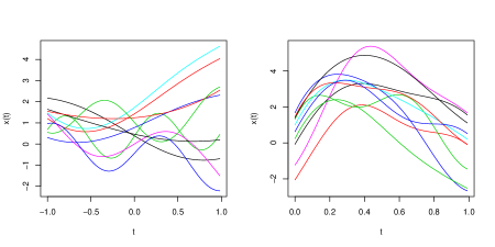
Figure 1: Ten random samples generated from Model 1 (left panel) and Model 2 (right panel).

We considered five regression functions:

• $r_{1}(X)=\left(\int_{\mathcal{I}}(X(t)-\mu(t))(\phi_{1}(t)+\phi_{2}(t))dt\right)^{1/3},$ where the first two FPCs ($\phi_{1}$ and $\phi_{2}$) and mean ($\mu$) for $M_{1}$ were calculated using a large sample of $x_{i},i=1,...,3000$, while for $M_{2}$ their true values were used,

• $r_{2}(X)=5\,\text{exp}\left(-\frac{1}{2}\lvert\int_{\mathcal{I}}x(t)\log(|x(t)|)dt\rvert\right),$

• $r_{3}(X)=5\,\text{logistic}\left(2\int_{\mathcal{I}}X(t)^{2}\text{sin}(2\pi t)dt\right),$ where $\text{logistic}(u)=1/(1+\text{exp}(-u))$, and

• $r_{4}(X)=5\left(\sqrt{\lvert\int_{\mathcal{I}_{1}}\text{cos}(2\pi t^{2})X(t)dt\rvert}+\sqrt{\lvert\int_{\mathcal{I}_{2}}\text{sin}(X(t))dt\rvert}\right),$ where $\mathcal{I}_{1}=[-1,0]$ and $\mathcal{I}_{2}=(0,1]$ for $M_{1}$, and $\mathcal{I}_{1}=[0,0.5]$ and $\mathcal{I}_{2}=(0.5,1]$ for $M_{2}$.

These regression functions were selected to represent a single-index model $(r_{1})$ and other nonlinear models ($r_{2}$, $r_{3}$, and $r_{4}$). To control the level of noise, we considered SNR = 5 and 20 as high and low noise levels and denoted them as $S_{1}$ and $S_{2}$, For each combination of the predictor model ($M$), regression function ($r$), and noise level ($S$), we generated i.i.d. samples $(x_{i},y_{i}),...,(x_{N},y_{N})$ of size $N=1600$. The dataset was randomly partitioned into a training set, a validation set, and a test set of size 400, 200, and 1000 respectively. In total, we simulated data from 16 settings, each defined as a combination $(M,r,S)$ from the set $\{M_{1},M_{2}\}\times\{r_{1},...,r_{4}\}\times\{S_{1},S_{2}\}$.

3.1 Implementation details

For each setting, we used 100 independently generated datasets and compared the performance of the following estimators:

• FLM1: functional linear regression with cubic B-splines (Hastie and Mallows, 1993),

• FLM2: functional linear regression with FPC scores (Cardot et al, 1999),

• FAM: functional additive models (Müller and Yao, 2008),

• FAME: functional adaptive model estimation (James and Silverman, 2005),

• FPPR: functional projection pursuit regression (Ferraty et al, 2013),

• FGAM: functional generalized additive models (McLean et al, 2014),

• RFgroove: random forests for grouped functional variable selection (Gregorutti et al, 2015)

• FRF: functional random forest with random intervals (Gregorutti et al, 2015)

• TFBoost(A,K): tree-based functional boosting with Type A trees, where each tree is specified with $K$ = 1, 2, or 3 indices, and

• TFBoost(B): tree-based functional boosting with Type B trees.

FLM1 and FLM2 are classical functional regression methods for linear models, and they use different bases to estimate the regression coefficients. For FLM1, we used cubic B-splines with 7 basis functions (3 evenly spaced interior knots), which was found to work generally well compared to using less or more interior knots. We penalized the second derivative of the coefficient and selected the penalization parameter to minimize the mean-squared-error (MSE) on the validation set. For FLM2, we used the top 4 FPCs required to explain 99% of the variance.

FAM constructs an additive estimator using FPC scores as predictors. We referred to its implementation in the fdapace package (Carroll et al, 2021) and used the Gaussian kernel to fit each additive component. Same as what we did for FLM2, the top 4 FPCs were used for FAM.

FAME estimates an extension of generalized additive models (GAM) to functional predictors. We used the code shared by the authors of James and Silverman (2005) and fitted the model using a Gaussian link function. FPPR follows the principle of projection pursuit regression and assumes an additive decomposition with each component being a functional single index model (FSIM). We implemented FPPR using the code to fit a single additive component shared by the authors of Ferraty et al (2013) and built an estimator by adding multiple functional single index estimators. Similarly to what was done with FLM1, for FPPR and FAME we used cubic B-splines with 7 functions (3 evenly spaced interior knots) as the basis. For both methods, we selected the number of additive components between 1 and 15 to minimize the MSE on the validation set. In our simulation settings, the performance of FAME and FPPR rarely improved beyond 15 additive components.

The implementation of FGAM is available from the refund package in R (Goldsmith et al, 2020). The method fits a model of the form

$$F(X)=\mu+\int G(X(t),t)dt,$$

where $\mu\in\mathbb{R}$, and $G$ is estimated using bivariate B-splines with roughness penalties. A restricted maximum likelihood approach is applied to select the parameter that penalizes the second order marginal differences of the basis (see the documentation of fgam in the refund package for details). We chose to use tensor-type bivariate cubic B-splines of dimensions 15 by 15. In all our settings, this choice ensured a stable fit and almost always resulted in the best performance compared to using other B-splines bases.

The method in RFgroove was originally proposed for computing importance measures for groups of functional variables (Gregorutti et al, 2015). Although the concept of grouped variable importance is not applicable to our case with a single functional predictor, we borrowed the idea to fit a random forest using projections on a functional basis as features. The R package RFgroove (Gregorutti, 2016) implements wavelet and FPC bases. However the discrete wavelet transform (DWT) requires data of length $2^{J}$ for some integer $J$, which was not applicable in our case, so we used the top FPC basis components that explain 99% of the variance. We adapted the code to obtain predicted values and used 500 trees to construct the random forest with the default control parameters of the function rpart that fits the trees.

The FRF approach of Möller et al (2016) randomly partitions the domain of the functional variables into intervals and uses the average of the function evaluations over these intervals as predictors in regression trees. Following Möller et al (2016), we used 500 regression trees to construct a random forest, sampled the lengths of the intervals from the exponential distribution, and selected the rate parameters from the values {1, 5, 10, 15, 20, 25, 30} in order to minimize the prediction error on the validation set.

For the proposed methods, we implemented TFBoost in R, including TFBoost(A.K) for positive integers $K$ and TFBoost(B). We fitted decision trees using the rpart package (Therneau and Atkinson, 2019) and performed optimization of TFBoost(A.K) using the Nelder_Mead function from the lme4 package (Bates et al, 2015). The code implementing our method is publicly available online at https://github.com/xmengju/TFBoost. To make a fair comparison with its alternatives, we used cubic B-splines with 7 functions (3 evenly spaced interior knots) as the basis for TFBoost methods, same as what we did for FLM1, FPPR, and FAME. We then orthonormalized the basis as required by Type A and Type B trees.

We studied the performance of TFBoost(A.K) with $K$ = 1,2, and 3; and TFBoost(B) using 200 random directions at each iteration. For each of these methods, the maximum depth ($d$) of the functional multi-index trees was fixed for all iterations. We experimented with $d\in\{1,2,3,4\}$ and for each method selected the value of $d$ that achieved the lowest MSE on the validation set at the early stopping time. We set the shrinkage parameter $\gamma$ to 0.05 and the maximum number of iterations $T_{\texttt{max}}$ to 1000.

As mentioned in Section 2.1.1, the estimation of a Type A tree may result in a non-convex optimization problem. To avoid suboptimal local minima, we fitted each Type A tree with multiple starting points. More specifically, we first uniformly sampled 30 points in the spherical coordinates system that satisfied the box constrains in (15) and ran the Nelder-Mead algorithm for 10 steps using each of the 30 points as the starting point. We then chose the five ending points with the lowest objective values and continued running the Nelder-Mead algorithm until convergence. Out of the five resulting estimates, we chose the one that minimized the objective function.

The results for all methods under consideration were evaluated in terms of the MSE on the test set ($\mathcal{T}$):

$$\text{MSE}=\frac{1}{|\mathcal{T}|}\sum_{i\in\mathcal{T}}(\hat{F}(x_{i})-y_{i})^{2}.$$ (21)

For TFBoost, the estimate $\hat{F}$ was reported at the early stopping time.

3.2 Results

For each combination of the regression function $(r_{1},...,r_{4})$ and the predictor model ($M_{1},M_{2}$), the results for the high noise ($S_{1}$) settings look very similar as those for the low noise ($S_{2}$) settings. In $S_{2}$ settings, the differences between estimators are more pronounced, showing a larger advantage of TFBoost(A.K) and TFBoost(B) over the others. We report here the results for $S_{1}$ settings and provide those for $S_{2}$ in the Appendix.

Figures 2, 3, 4 and 5 show the MSEs on the test sets for $r_{1}$ to $r_{4}$ respectively. Since FLM1, FLM2, FAM, and RFgroove tend to produce very large errors, to be able to visualize the differences among the other methods, we excluded them from the figures and reported the summary statistics of their MSEs in the Appendix. As expected, the linear estimators (FLM1 and FLM2) do not work well since $r_{1}$ to $r_{4}$ are nonlinear functions. FAM and RFgroove also perform poorly, likely due to using FPCs as the projection direction to construct features, making them less flexible compared with using random features (like those generated by FRF) or estimating the projection directions based on the data.

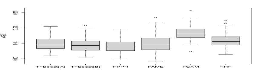
(a) $M_{1}$

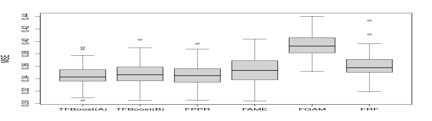
(b) $M_{2}$

Figure 2: Boxplots of MSEs on test sets from 100 runs of the experiment with data generated from ($r_{1}$, $M_{1}$, $S_{1}$) in panel (a) and ($r_{1}$, $M_{2}$, $S_{1}$) in panel (b).

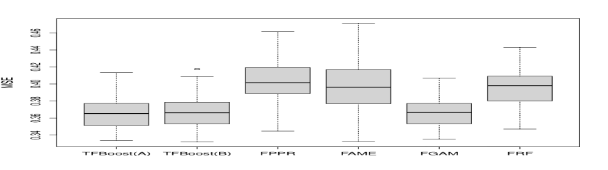
(a) $M_{1}$

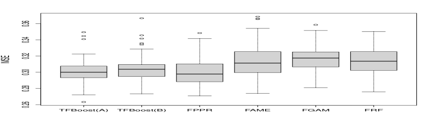
(b) $M_{2}$

Figure 3: Boxplots of MSEs on test sets from 100 runs of the experiment with data generated from ($r_{2}$, $M_{1}$, $S_{1}$) in panel (a) and ($r_{2}$, $M_{2}$, $S_{1}$) in panel (b).

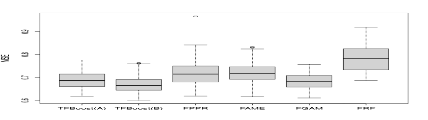
(a) $M_{1}$

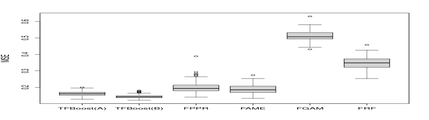
(b) $M_{2}$

Figure 4: Boxplots of MSEs on test sets from 100 runs of the experiment with data generated from ($r_{3}$, $M_{1}$, $S_{1}$) in panel (a) and ($r_{3}$, $M_{2}$, $S_{1}$) in panel (b).

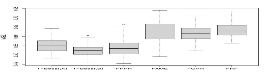
(a) $M_{1}$

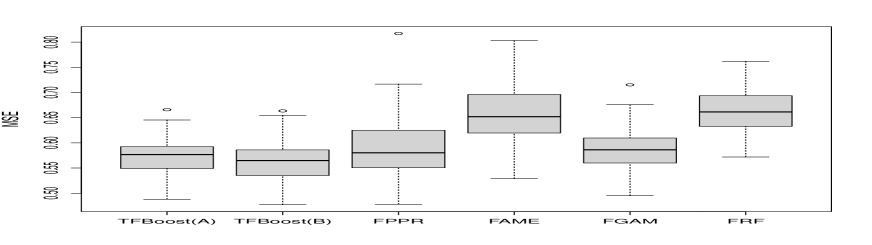
(b) $M_{2}$

Figure 5: Boxplots of MSEs on test sets from 100 runs of the experiment with data generated from ($r_{4}$, $M_{1}$, $S_{1}$) in panel (a) and ($r_{4}$, $M_{2}$, $S_{1}$) in panel (b).

In each figure, panel (a) corresponds to data with the predictors generated from $M_{1}$ and panel (b) to those from $M_{2}$. Each panel shows the boxplot of MSEs on the test sets from 100 independent runs of the experiment. For TFBoost(A.K), we show the MSEs for the value of $K$ that gave the best results on the test sets, and include the rest in the Appendix. In the case of a tie we picked the simpler model (one with a smaller $K$). As a result, we selected

• $K=2$ for all $r_{1}$ and $r_{2}$ settings, and $(r_{3},M_{2})$,

• $K=3$ for all $r_{4}$ settings and $(r_{3},M_{1})$.

The label TFBoost(A) on the x-axis in each figure represents TFBoost(A.K) with $K$ selected for the corresponding setting.

In general, TFBoost(A) and TFBoost(B) show stable and remarkable predictive performance in all these figures, with either or both achieving the lowest or second lowest average test MSEs across all methods. In contrast, the performance of FPPR, FAME, and FGAM heavily depends on the regression function as well as the predictor model. For example, in panel (a) of Figure 3 where $X$ was generated from $M_{1}$, FPPR produces the worst errors compared to the other methods. However, when $X$ followed $M_{2}$ in panel (b), FPPR becomes one of the best. The opposite holds for FGAM, being among the best in panel (a) and the worst in panel (b). Similarly in Figure 4, the performance of FGAM differs greatly in $M_{1}$ and $M_{2}$ settings. In Figures 2 and 5, the performances of FAME and FGAM are similar in both $M_{1}$ and $M_{2}$ settings, but they differ substantially across figures. FGAM produces significantly worse errors compared to FAME in Figure 2, whereas in Figure 5 we observe the opposite. The performance of FRF is at the bottom in all settings, being the worst or the second worst method. We think that this is due to its features constructed using the average of functional values across intervals fail to carry sufficient information to predict the response with high accuracy.

It is worth noting that TFBoost methods are close to their alternatives in terms of test errors when the true model matches the one on which the other methods are based. For example, in Figure 2 TFBoost(A) and TFBoost(B) produce similar errors as FPPR, where the regression function $r_{2}$ matches with the true model of FPPR specified with a single additive component. In other cases where the alternatives deviate from the true model, TFBoost(A) and TFBoost(B) usually show the lowest errors and their performances are stable regardless of the setting. This illustrates the flexibility of our method, which helps to achieve low prediction errors without posing strong assumptions on the target function.

For each simulated setting, we also analyzed the performance of TFBoost by plotting the test errors averaged from 100 runs of the experiment versus the number of iterations. To make it easier to take the averages for each method, for each run, we let the test errors for the iterations past the early stopping time ($T_{\text{stop}}$) to have the same value as the one obtained at $T_{\text{stop}}$. Figure 6 shows an example of such figures for ($r_{1}$, $M_{1}$, $S_{1}$) and ($r_{1}$, $M_{1}$, $S_{1}$) settings. The summary statistics of $T_{\text{stop}}$ and the selected tree depths $d$ are provided in Table 1. We can see that the test errors of TFBoost drop quickly within the first 100 iterations. The same pattern can be observed for the other settings, the results of which can be found in the Appendix.

(a) $M_{1}$

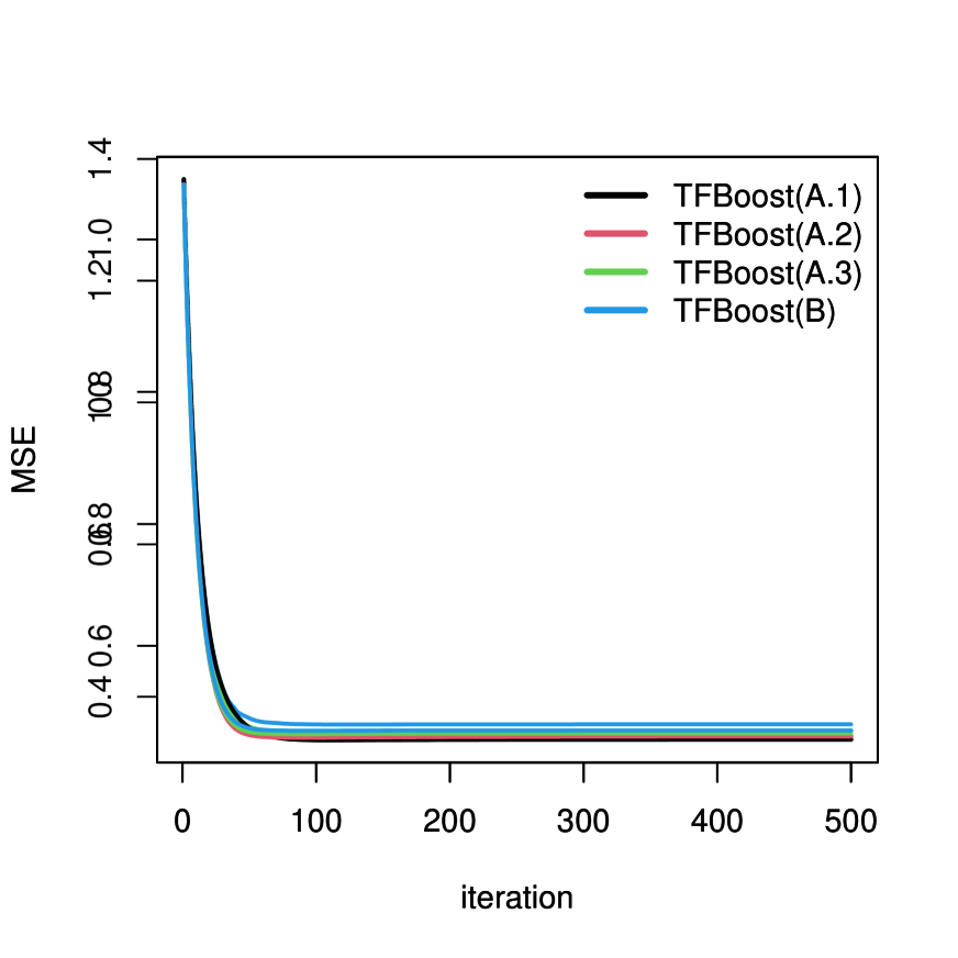
(b) $M_{2}$

Figure 6: Test MSEs averaged from 100 runs of the experiment for TFBoost for data generated from ($r_{1}$, $M_{1}$, $S_{1}$) in panel (a) and ($r_{1}$, $M_{2}$, $S_{1}$) in panel (b).

	$M_{1}$		$M_{2}$
	$T_{\text{stop}}$	$d$	$T_{\text{stop}}$	$d$
TFBoost(A.1)	127.75 (74.22)	1.58 (0.77)	149.05 (130.43)	1.77 (0.98)
TFBoost(A.2)	121.02 (82.62)	1.55 (0.78)	120.74 (76.94)	1.67 (0.96)
TFBoost(A.3)	113.52 (54.25)	1.40 (0.65)	121.83 (94.96)	1.64 (0.82)
TFBoost(B)	96.05 (38.05)	1.32 (0.66)	107.63 (50.49)	1.32 (0.60)

Table 1: Summary statistics of the early stopping times ($T_{\text{stop}}$) and tree depths ($d$) selected by TFBoost for data generated from ($r_{1}$, $M_{1}$, $S_{1}$) and ($r_{1}$, $M_{2}$, $S_{1}$); displayed in the form of mean (sd).

So far we have focused on the performance of TFBoost in nonlinear settings since the base learners are nonlinear. In the Appendix, we provide also results for an experiment fitting TFBoost methods with data generated from a linear model and comparing them with alternatives considered previously. As expected, the linear estimators FLM1, FLM2 outperform the others. For FGAM, the linear regression function matches with its model assumptions, which explains its good performance in linear settings. We note that the test errors of TFBoost(A) are only slightly worse than those produced by linear estimators: about 5% worse in the $M_{1}$ setting, and about 7% worse in the $M_{2}$ setting. This implies that even though TFBoost is an estimator for possibly nonlinear regression functions, we do not lose much applying it to data generated from linear models.

4 German electricity data

To illustrate the use of TFBoost, we analyzed a data set consisting of electricity spot prices traded at the European Energy Exchange (EEX) in Leipzig and electricity demand reported by the European Network of Transmission System Operators for Electricity from January 1st 2006 to September 30th 2008. On each day, electricity spot prices and demands were recorded hourly and represented as vectors of dimension 24. Our objective is to predict the daily average of electricity demand using hourly electricity spot prices. The whole dataset is available from the on-line supplementary materials of Liebl et al (2013). To avoid days with known atypical price or demand values affecting our analysis, we removed weekends and holidays and analyzed data collected on the remaining 638 days. For each of these days, we view the hourly electricity spot prices as discretized evaluations of a smooth price function.

We considered methods of TFBoost(A,K) with $K$ = 1, 2, and 3, TFBoost(B), as well as their alternatives FLM1, FLM2, FAM, FPPR, FAME, FGAM, RFgroove, and FRF. To adjust for potential seasonality effects, we created a “day of the year” variable defined as the number of days from January 1st of the year in which the data were collected. In order to compare the results before and after adjusting for seasonality, our analysis consisted of two parts: (1) predicting daily electricity demand with hourly electricity prices only, and (2) with both hourly electricity prices and the “day of the year” variable.

In part (1), all methods under consideration were specified in the same way as in Section 3.1. In part (2), we added “day of the year” as an additional predictor to all methods and adjusted their algorithms accordingly. For TFBoost methods, at every boosting iteration, we added “day of the year” as an additional variable to the functional multi-index tree. For the competitors, we included the scalar predictor in the model following the same approach as we did for the functional predictor. We added “day of the year” as a linear term in FLM1 and FLM2, and as a nonparametric term in FAM, FPPR, FAME, FGAM, RFgroove, and FRF. For each of FAM and FPPR, we first calculated the estimator in the same way as in part (1) and obtained the residuals. Then we added to the part (1) estimator a Nadaraya-Watson estimator with Gaussian kernel fitted to the residuals using “day of the year” as the predictor. For FAME and FGAM we specified a smooth term on “day of the year” represented as penalized cubic splines (Wood, 2017). For RFgroove and FRF, we added “day of the year” as an additional predictor to each regression tree used to construct random forests. Other than adding this additional predictor, the other parameters and fitting procedures were kept the same as in part (1).

We randomly partitioned the data into a training set (60%), a validation set (20%), and a test set (20%). As in Section 3, we fitted each model using the training and validation sets and recorded MSE on the test set. The validation set was used to choose the regularization parameter of FLM1, the number of additive components of FAM and FPPR, the rate parameters to generate the intervals for FRF, and the maximum tree depth and early stopping time of TFBoost(A,1),TFBoost(A,2), TFBoost(A,3), and TFBoost(B).

To reduce the variability introduced by partitioning the data, we repeated the experiment with 100 random data splits. Figures 7 and 8 show test MSEs obtained from 100 random data splits in part (1) and (2) of the experiment respectively. The summary statistics of these test MSEs for all methods are provided in the Appendix. To better reveal the differences between the estimators under consideration, in each figure the y-axis is truncated and represents test MSE $\times 10^{-6}$. We also excluded FLM1, FLM2, and FAM from the figures since they performed very poorly in part(1) and part(2).

In both figures, TFBoost(A.1), TFBoost(A.2), TFBoost(A.3), and TFBoost(B) show superior performance compared to their alternatives. They achieve the lowest errors with the smallest standard errors. In Figure 7, we observe that TFboost(B) produces the smallest test errors, substantially better than FLM1,FLM2, FAM, FGAM, and FPPR, and slightly better than FRF and RFgroove.

Comparing Figure 8 with Figure 7, we observe improvements in test errors for all methods except for FLM1. This implies the importance of adjusting for seasonality when predicting the electricity demand, which is likely due to higher electricity usage in the summer for cooling and in the winter for heating. In Figure 8, TFBoost(A.1), TFBoost(A.2), TFBoost(A.3) produce very similar results, and TFBoost(A.2) outperforms the other two by a small margin in terms of the average test MSE.

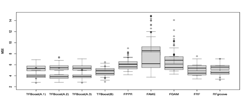
Figure 7: Boxplot of test MSEs obtained from 100 random splits of the data from part (1) of the experiment. The unit of y-axis is $10^{-6}$.

Figure 8: Boxplot of test MSEs obtained from 100 random splits of the data from part (2) of the experiment. The unit of y-axis is $10^{-6}$.

5 Conclusion and future work

In this paper we have proposed a novel boosting method for regression with a functional explanatory variable. Our approach uses functional multi-index trees as base learners, which offer flexibility and are relatively easy to fit. Compared with widely studied single index estimators, our multi-index estimator enables modelling possible interactions between indices, allowing us to better approximate complex regression functions. Through extensive numerical experiments, we demonstrate that our method consistently produces one of the lowest prediction errors across different settings, while available alternatives can be seriously affected by model misspecification. In addition, TFBoost with Type B learners exhibits significant computational advantages over kernel-based methods, being able to provide accurate predictions at a much lower cost.

The methodology of TFBoost suggests a number of interesting areas for future work. First, we formulated the regression problem with a single functional predictor, but in principle, it could also be extended to multiple predictors, functional or scalar. This can be achieved by including indices calculated from multiple predictors, either allowing each index to be associated with all predictors or one of the predictors. If there are many predictors, this approach may be computationally difficult and can result in unstable estimators when the sample size is small. In this situation, we need to assume sparsity in the functional space, which means that some but not all predictors are related to the response. Group penalties with projections on each predictor being a group can be considered to enable variable selection. Second, in our experiments we only studied TFBoost applied with the squared loss. In cases where data contain outliers, it will be useful to consider fitting our method with different loss functions, for example, Huber’s or Tukey’s loss. Finally, in this paper we focused on functional predictors observed at many time points without measurement errors. In practice, one may encounter situations where only very few and possibly noisy measurements of the predictor function are available. In this case, smoothing each predictor curve provides unreliable approximations and makes them poor inputs to TFBoost. It may be more advisable to borrow strength across curves, for example, fitting TFBoost to curves reconstructed using FPCA (Yao et al (2005) and Boente and Salibian-Barrera (2021)).

6 Acknowledgements

The authors would like to thank Professors James and Ferraty for sharing the code used in their papers (James and Silverman (2005) and Ferraty et al (2013)). In addition, we would like to thank two anonymous referees and an Associate Editor for their constructive comments on an earlier version of this work that resulted in a notably improved paper.

7 Statements and Declarations

This research was supported by the Natural Sciences and Engineering Research Council of Canada [Discovery Grant RGPIN-2016-04288]. The authors have no competing interests to declare that are relevant to the content of this article.

APPENDICES

Proof of 1 in Section 2.1.1.

Proof.

It is clear that if $\{\beta_{1},...,\beta_{K}\}=\{(-1)^{l_{1}}\eta_{1},...,(-1)^{l_{K}}\eta_{K}\}$ for some $l_{1},...,l_{K}\in\{0,1\}$, then $g=\tilde{g}$. Therefore, it suffices to show that $\{\beta_{1},...,\beta_{K}\}=\{(-1)^{l_{1}}\eta_{1},...,(-1)^{l_{K}}\eta_{K}\}$ for some $l_{1},...,l_{K}\in\{0,1\}$. We prove that if there do not exist $l_{1},...,l_{K}$ for the two sets to be equal, there exists a set of indices for which (12) is a constant function and thus contradicts 2.

For simplicity, we let $\tilde{\eta}_{j}=(-1)^{l_{j}}\eta_{j}$. If for any $l_{1},...,l_{K}$, $\{\beta_{1},...,\beta_{K}\}\neq\{\tilde{\eta}_{1},...,\tilde{\eta}_{K}\}$, we match two sets so that the same vectors $\beta_{j}$ and $\tilde{\eta}_{j}$ align with each other. We let $S=\{\beta_{1},...,\beta_{K}\}\cap\{\tilde{\eta}_{1},...,\tilde{\eta}_{K}\}$, $\beta_{j}=\tilde{\eta}_{j}$, for $j=1,...,|S|$ and $\beta_{j}\notin\{\tilde{\eta}_{1},...,\tilde{\eta}_{K}\}$, for $j=|S|+1,...,K$, and $|S|<K$. By 2, there exist a $x_{0}$ for $J={|S|+1,...,K}$, (12) is not a constant function.

By (13), 1 and 2, for any $t_{1},...,t_{K}\in(-\delta,\delta)$

$$h(\langle x_{0},\beta_{1}\rangle+t_{1},...,\langle x_{0},\beta_{K}\rangle+t_{K}) =h(\langle x_{0}+t_{1}\beta_{1},\beta_{1}\rangle,...,\langle x_{0}+t_{K}\beta_{K}\rangle,\beta_{K})$$

$$=\tilde{h}(\langle x_{0}+t_{1}\beta_{1},\eta_{1}\rangle,...,\langle x_{0}+t_{K}\beta_{K},\eta_{K}\rangle)$$

$$=\tilde{h}(\langle x_{0},\eta_{1}\rangle+t_{1}\langle\beta_{1},\eta_{1}\rangle,...,\langle x_{0},\eta_{K}\rangle+t_{K}\langle\beta_{K},\eta_{K}\rangle)$$

and similarly

$$\tilde{h}(\langle x_{0},\eta_{1}\rangle+t_{1},...,\langle x_{0},\eta_{K}\rangle+t_{K}) =\tilde{h}(\langle x_{0}+t_{1}\eta_{1},\eta_{1}\rangle,...,\langle x_{0}+t_{K}\eta_{K},\eta_{K}\rangle)$$

$$=h(\langle x_{0}+t_{1}\eta_{1},\beta_{1}\rangle,...,\langle x_{0}+t_{K}\eta_{K},\beta_{K}\rangle)$$

$$=h(\langle x_{0},\beta_{1}\rangle+t_{1}\langle\beta_{1},\eta_{1}\rangle,...,\langle x_{0},\beta_{K}\rangle+t_{K}\langle\beta_{K},\eta_{K}\rangle)$$

By Cauchy-Schwarz inequality and 1, $(\langle\beta_{j},\eta_{j}\rangle)^{2}=1$ for $j=1,...,|S|$ and $(\langle\beta_{j},\eta_{j}\rangle)^{2}<1$ for $j=|S+1|,...,K$. For any $t_{1},...,t_{K}\in(-\delta,\delta)$,

$$h(\langle x_{0},\beta_{1}\rangle+t_{1},...,\langle x_{0},\beta_{K}\rangle+t_{K}) =\tilde{h}(\langle x_{0},\eta_{1}\rangle+t_{1}\langle\beta_{1},\eta_{1}\rangle,...,\langle x_{0},\eta_{K}\rangle+t_{K}\langle\beta_{K},\eta_{K}\rangle)$$

$$=h(\langle x_{0},\beta_{1}\rangle+t_{1}\langle\beta_{1},\eta_{1}\rangle^{2},...,\langle x_{0},\beta_{K}\rangle+t_{K}\langle\beta_{K},\eta_{K}\rangle^{2})$$

$$\vdots$$

$$=h(\langle x_{0},\beta_{1}\rangle+t_{1}\langle\beta_{1},\eta_{1}\rangle^{2n},...,\langle x_{0},\beta_{K}\rangle+t_{K}\langle\beta_{K},\eta_{K}\rangle^{2n})$$

$$\vdots$$

$$=h(\langle x_{0},\beta_{1}\rangle+t_{1}I_{1},...,\langle x_{0},\beta_{K}\rangle+t_{K}I_{K})$$ (22)

where $I_{j}=1$ for $j=1,...,|S|$ and $I_{j}=0$ for $j=|S+1|,...,|K|$.

Let $x=x_{0}+te$ for any unit function $e\in L^{2}(\mathcal{I})$, $\lVert e\rVert=1$ and $t\in(-\delta,\delta)$. Then $x$ fills the space of $B(x_{0},\delta)$. For $j=1,...,K$, we define

$$L_{j}(x) =(1-I_{j})x+I_{j}x_{0}$$

$$=(1-I_{j})(x_{0}+te)+I_{j}x_{0}$$

$$=x_{0}+(1-I_{j})te$$

$$h(\langle L_{1}(x),\beta_{1}\rangle,...,\langle L_{K}(x),\beta_{K}\rangle) =h(\langle x_{0}+(1-I_{1})te,\beta_{1}\rangle,...,\langle x_{0}+(1-I_{K})te,\beta_{K}\rangle)$$

$$=h(\langle x_{0},\beta_{1}\rangle+\langle(1-I_{1})te,\beta_{1}\rangle,...,\langle x_{0},\beta_{K}\rangle+$$

$$\langle(1-I_{K})te,\beta_{K}\rangle),\text{by}\ \eqref{myeq}$$

$$=h(\langle x_{0},\beta_{1}\rangle+\langle I_{1}(1-I_{1})te,\beta_{1}\rangle,...,\langle x_{0},\beta_{K}\rangle+$$

$$\langle I_{K}(1-I_{K})te,\beta_{K}\rangle)$$

$$=h(\langle x_{0},\beta_{1}\rangle,...,\langle x_{0},\beta_{K}\rangle),$$

which is a constant function of $x$ and that contradicts 2. ∎

Appendix B

The summary statistics of test MSEs from 100 independent runs of the simulation are provided in Tables 2, 5, 8 and 11, with bold font indicating the lowest two average test errors in each setting. Summary statistics of the tree depths selected by TFBoost are provided in Tables 3, 6, 9 and 12, and for the early stopping times for TFBoost are provided in Tables 4, 7, 10 and 13.

	SNR = 20		SNR = 5
	$M_{1}$	$M_{2}$	$M_{1}$	$M_{2}$
TFBoost(A.1)	0.118 (0.006)	0.090 (0.004)	0.449 (0.021)	0.347 (0.016)
TFBoost(A.2)	0.118 (0.006)	0.090 (0.004)	0.449 (0.022)	0.345 (0.016)
TFBoost(A.3)	0.120 (0.005)	0.090 (0.004)	0.450 (0.020)	0.347 (0.016)
TFBoost(B)	0.116 (0.005)	0.091 (0.004)	0.445 (0.022)	0.347 (0.016)
FLM1	0.218 (0.009)	0.200 (0.008)	0.534 (0.022)	0.445 (0.019)
FLM2	0.219 (0.008)	0.200 (0.008)	0.534 (0.021)	0.446 (0.019)
FAM	0.308 (0.055)	0.190 (0.010)	0.624 (0.061)	0.438 (0.021)
FPPR	0.113 (0.006)	0.089 (0.005)	0.440 (0.021)	0.347 (0.018)
FAME	0.118 (0.008)	0.094 (0.007)	0.448 (0.026)	0.353 (0.021)
FGAM	0.151 (0.007)	0.134 (0.006)	0.483 (0.022)	0.393 (0.018)
FRF	0.138 (0.008)	0.113 (0.006)	0.459 (0.022)	0.360 (0.019)
RFGroove	0.179 (0.011)	0.165 (0.010)	0.521 (0.023)	0.423 (0.021)

Table 2: Summary statistics of test errors for data generated from $r_{1}$; displayed in the form of mean (sd).

	SNR = 20		SNR = 5
	$M_{1}$	$M_{2}$	$M_{1}$	$M_{2}$
TFBoost(A.1)	1.59 (0.64)	1.98 (0.88)	1.58 (0.77)	1.77 (0.98)
TFBoost(A.2)	1.44 (0.61)	1.71 (0.84)	1.55 (0.78)	1.67 (0.96)
TFBoost(A.3)	1.54 (0.63)	1.74 (0.79)	1.40 (0.65)	1.64 (0.82)
TFBoost(B)	1.51 (0.73)	1.52 (0.66)	1.32 (0.66)	1.32 (0.60)

Table 3: Summary statistics of the tree depths selected by TFBoost for data generated from $r_{1}$; displayed in the form of mean (sd).

	SNR = 20		SNR = 5
	$M_{1}$	$M_{2}$	$M_{1}$	$M_{2}$
TFBoost(A.1)	184.36 (148.77)	179.12 (140.80)	127.75 (74.22)	149.05 (130.43)
TFBoost(A.2)	159.15 (104.41)	160.64 (124.48)	121.02 (82.62)	120.74 (76.94)
TFBoost(A.3)	151.91 (68.41)	160.39 (122.58)	113.52 (54.25)	121.83 (94.96)
TFBoost(B)	120.24 (50.50)	140.08 (104.60)	96.05 (38.05)	107.63 (50.49)

Table 4: Summary statistics of the early stoping times $T_{\text{stop}}$ selected by TFBoost methods for data generated from $r_{1}$; displayed in the form of mean (sd).

	SNR = 20		SNR = 5
	$M_{1}$	$M_{2}$	$M_{1}$	$M_{2}$
TFBoost(A.1)	0.143 (0.009)	0.091 (0.005)	0.371 (0.018)	0.302 (0.014)
TFBoost(A.2)	0.133 (0.008)	0.089 (0.005)	0.365 (0.018)	0.301 (0.014)
TFBoost(A.3)	0.130 (0.009)	0.089 (0.005)	0.365 (0.019)	0.301 (0.014)
TFBoost(B)	0.124 (0.008)	0.091 (0.005)	0.366 (0.019)	0.304 (0.015)
FLM1	0.610 (0.032)	0.177 (0.011)	0.815 (0.040)	0.376 (0.018)
FLM2	0.611 (0.032)	0.176 (0.011)	0.816 (0.040)	0.376 (0.017)
FAM	0.352 (0.076)	0.137 (0.012)	0.560 (0.081)	0.337 (0.017)
FPPR	0.155 (0.014)	0.092 (0.006)	0.402 (0.024)	0.300 (0.017)
FAME	0.148 (0.016)	0.099 (0.010)	0.397 (0.029)	0.313 (0.020)
FGAM	0.150 (0.009)	0.113 (0.008)	0.366 (0.017)	0.316 (0.014)
FRF	0.192 (0.011)	0.118 (0.008)	0.394 (0.020)	0.313 (0.015)
RFGroove	0.216 (0.012)	0.178 (0.015)	0.433 (0.021)	0.382 (0.021)

Table 5: Summary statistics of test errors for data generated from $r_{2}$; displayed in the form of mean (sd).

	SNR = 20		SNR = 5
	$M_{1}$	$M_{2}$	$M_{1}$	$M_{2}$
TFBoost(A.1)	1.75 (0.72)	2.17 (1.02)	1.79 (0.83)	2.20 (1.06)
TFBoost(A.2)	2.72 (0.81)	2.85 (0.90)	2.46 (1.09)	2.35 (1.05)
TFBoost(A.3)	3.07 (0.82)	2.95 (0.94)	2.53 (1.05)	2.35 (0.91)
TFBoost(B)	3.34 (0.68)	2.66 (1.00)	2.72 (1.05)	1.99 (0.92)

Table 6: Summary statistics of the tree depths selected by TFBoost for data generated from $r_{2}$; displayed in the form of mean (sd).

	SNR = 20		SNR = 5
	$M_{1}$	$M_{2}$	$M_{1}$	$M_{2}$
TFBoost(A.1)	968.39 (64.41)	596.26 (263.95)	699.66 (265.11)	262.33 (196.84)
TFBoost(A.2)	863.20 (168.48)	351.35 (268.34)	481.17 (274.79)	198.20 (172.81)
TFBoost(A.3)	812.06 (216.51)	318.31 (253.23)	486.76 (292.74)	182.57 (154.14)
TFBoost(B)	608.15 (269.46)	255.58 (226.69)	318.60 (261.46)	154.19 (121.87)

Table 7: Summary statistics of the early stoping times $T_{\text{stop}}$ selected by TFBoost methods for data generated from $r_{2}$; displayed in the form of mean (sd).

	SNR = 20		SNR = 5
	$M_{1}$	$M_{2}$	$M_{1}$	$M_{2}$
TFBoost(A.1)	0.220 (0.014)	0.082 (0.013)	0.694 (0.041)	0.160 (0.014)
TFBoost(A.2)	0.216 (0.014)	0.080 (0.012)	0.693 (0.037)	0.159 (0.014)
TFBoost(A.3)	0.214 (0.014)	0.079 (0.012)	0.688 (0.035)	0.161 (0.014)
TFBoost(B)	0.195 (0.011)	0.061 (0.009)	0.670 (0.035)	0.143 (0.011)
FLM1	1.358 (0.061)	0.689 (0.038)	1.788 (0.086)	0.759 (0.039)
FLM2	1.352 (0.065)	0.689 (0.038)	1.781 (0.089)	0.759 (0.039)
FAM	0.947 (0.117)	0.501 (0.042)	1.383 (0.129)	0.572 (0.044)
FPPR	0.237 (0.028)	0.114 (0.033)	0.718 (0.056)	0.201 (0.037)
FAME	0.231 (0.023)	0.092 (0.021)	0.720 (0.048)	0.188 (0.028)
FGAM	0.219 (0.013)	0.438 (0.029)	0.683 (0.036)	0.512 (0.031)
FRF	0.370 (0.041)	0.279 (0.037)	0.783 (0.053)	0.348 (0.037)
RFGroove	0.459 (0.033)	0.314 (0.032)	0.913 (0.051)	0.386 (0.033)

Table 8: Summary statistics of test errors for data generated from $r_{3}$; displayed in the form of mean (sd).

	SNR = 20		SNR = 5
	$M_{1}$	$M_{2}$	$M_{1}$	$M_{2}$
TFBoost(A.1)	1.16 (0.39)	1.08 (0.27)	1.39 (0.62)	1.06 (0.24)
TFBoost(A.2)	1.81 (0.87)	1.43 (0.57)	1.88 (0.95)	1.47 (0.73)
TFBoost(A.3)	1.80 (0.90)	1.76 (0.88)	1.81 (0.90)	1.71 (0.86)
TFBoost(B)	2.97 (0.88)	3.12 (0.73)	2.22 (0.96)	2.97 (0.88)

Table 9: Summary statistics of the tree depths selected by TFBoost for data generated from $r_{3}$; displayed in the form of mean (sd).

	SNR = 20		SNR = 5
	$M_{1}$	$M_{2}$	$M_{1}$	$M_{2}$
TFBoost(A.1)	950.58 (116.79)	977.61 (58.60)	582.67 (245.51)	889.96 (136.17)
TFBoost(A.2)	818.94 (237.53)	926.64 (134.11)	459.91 (274.04)	765.63 (252.55)
TFBoost(A.3)	780.60 (257.62)	898.08 (158.45)	441.94 (260.47)	712.90 (264.68)
TFBoost(B)	304.22 (238.92)	435.92 (257.85)	232.23 (181.15)	231.74 (200.35)

Table 10: Summary statistics of the early stoping times $T_{\text{stop}}$ selected by TFBoost methods for data generated from $r_{3}$; displayed in the form of mean (sd).

	SNR = 20		SNR = 5
	$M_{1}$	$M_{2}$	$M_{1}$	$M_{2}$
TFBoost(A.1)	0.252 (0.020)	0.271 (0.027)	0.570 (0.038)	0.583 (0.037)
TFBoost(A.2)	0.237 (0.019)	0.262 (0.025)	0.558 (0.033)	0.575 (0.035)
TFBoost(A.3)	0.226 (0.019)	0.260 (0.026)	0.550 (0.033)	0.574 (0.036)
TFBoost(B)	0.196 (0.016)	0.248 (0.026)	0.524 (0.030)	0.563 (0.039)
FLM1	1.438 (0.071)	0.586 (0.036)	1.712 (0.080)	0.857 (0.047)
FLM2	1.454 (0.071)	0.586 (0.036)	1.725 (0.079)	0.855 (0.045)
FAM	0.898 (0.145)	0.525 (0.042)	1.174 (0.148)	0.795 (0.051)
FPPR	0.209 (0.024)	0.261 (0.046)	0.540 (0.048)	0.588 (0.057)
FAME	0.308 (0.044)	0.339 (0.044)	0.628 (0.054)	0.657 (0.059)
FGAM	0.300 (0.022)	0.290 (0.032)	0.618 (0.037)	0.587 (0.042)
FRF	0.368 (0.027)	0.402 (0.031)	0.635 (0.037)	0.662 (0.038)
RFGroove	0.487 (0.037)	0.481 (0.039)	0.777 (0.049)	0.758 (0.049)

Table 11: Summary statistics of test errors for data generated from $r_{4}$; displayed in the form of mean (sd).

	SNR = 20		SNR = 5
	$M_{1}$	$M_{2}$	$M_{1}$	$M_{2}$
TFBoost(A.1)	2.19 (0.79)	1.98 (0.51)	2.10 (0.83)	1.74 (0.66)
TFBoost(A.2)	2.58 (0.71)	2.40 (0.62)	2.22 (0.94)	2.21 (0.91)
TFBoost(A.3)	2.50 (0.69)	2.47 (0.67)	2.15 (0.91)	2.12 (0.89)
TFBoost(B)	3.06 (0.79)	2.45 (0.69)	2.85 (0.95)	2.30 (0.86)

Table 12: Summary statistics of the tree depths selected by TFBoost for data generated from $r_{4}$; displayed in the form of mean (sd).

	SNR = 20		SNR = 5
	$M_{1}$	$M_{2}$	$M_{1}$	$M_{2}$
TFBoost(A.1)	962.39 (55.28)	902.47 (134.21)	781.78 (243.59)	772.73 (233.61)
TFBoost(A.2)	920.57 (131.91)	844.47 (180.19)	682.31 (299.37)	603.05 (317.61)
TFBoost(A.3)	870.27 (181.13)	810.42 (233.13)	644.36 (304.11)	647.26 (326.90)
TFBoost(B)	527.76 (263.12)	653.43 (261.88)	295.81 (256.69)	417.91 (298.59)

Table 13: Summary statistics of the early stoping times $T_{\text{stop}}$ selected by TFBoost methods for data generated from $r_{4}$; displayed in the form of mean (sd).

Figures 9, 10, 11 and 12 show the test MSEs averaged over 100 runs of the experiment versus the number of iterations for TFBoost. For the convenience of taking the averages, for each run, we let the test errors for the iterations past the early stopping time to keep the same test error as the one obtained at the early stopping time. It can be observed from figures that the test errors usually drop quickly within 100 iterations.

Figure 9: Test MSEs averaged from 100 runs of the experiment for TFBoost in $r_{1}$ settings

Figure 10: Test MSEs averaged from 100 runs of the experiment for TFBoost in $r_{2}$ settings

Figure 11: Test MSEs averaged from 100 runs of the experiment for TFBoost in $r_{3}$ settings

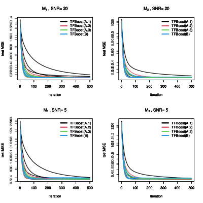
Figure 12: Test MSEs averaged from 100 runs of the experiment for TFBoost in $r_{4}$ settings

Appendix C

We consider another regression function that is linear:

$$r_{5}(X)=\int_{\mathcal{I}}\left(\text{sin}\left(\frac{3}{2}\pi t\right)+\text{sin}\left(\frac{1}{2}\pi t\right)\right)X(t)dt.$$

The other specifications of the model remain the same as described in Section 3. Table 14 include the summary statistics of test MSEs from 100 independent runs of the simulation, with bold font indicating the lowest two average test errors in each setting. Table 15 and Table 16 include the summary statistics of the tree depths and early stopping times selected by TFBoost methods.

	SNR = 20		SNR = 5
	$M_{1}$	$M_{2}$	$M_{1}$	$M_{2}$
TFBoost(A.1)	0.105 (0.005)	0.035 (0.002)	0.415 (0.019)	0.132 (0.006)
TFBoost(A.2)	0.107 (0.005)	0.035 (0.002)	0.419 (0.019)	0.133 (0.006)
TFBoost(A.3)	0.108 (0.005)	0.035 (0.002)	0.418 (0.019)	0.134 (0.006)
TFBoost(B)	0.109 (0.005)	0.037 (0.002)	0.420 (0.020)	0.136 (0.006)
FLM1	0.100 (0.005)	0.031 (0.001)	0.398 (0.018)	0.124 (0.006)
FLM2	0.099 (0.004)	0.031 (0.001)	0.395 (0.017)	0.123 (0.005)
FAM	0.191 (0.044)	0.033 (0.003)	0.490 (0.053)	0.126 (0.006)
FPPR	0.102 (0.005)	0.033 (0.002)	0.407 (0.022)	0.128 (0.006)
FAME	0.102 (0.005)	0.032 (0.002)	0.408 (0.021)	0.128 (0.007)
FGAM	0.099 (0.004)	0.031 (0.001)	0.396 (0.017)	0.123 (0.005)
FRF	0.150 (0.010)	0.050 (0.004)	0.442 (0.021)	0.140 (0.007)
RFGroove	0.150 (0.008)	0.100 (0.009)	0.469 (0.021)	0.194 (0.012)

Table 14: Summary statistics of test errors for data generated from $r_{5}$; displayed in the form of mean (sd).

	SNR = 20		SNR = 5
	$M_{1}$	$M_{2}$	$M_{1}$	$M_{2}$
TFBoost(A.1)	3.03 (0.88)	3.33 (0.79)	2.57 (1.07)	3.05 (0.89)
TFBoost(A.2)	2.63 (0.86)	3.22 (0.88)	2.23 (0.97)	2.61 (1.00)
TFBoost(A.3)	2.34 (0.86)	3.20 (0.72)	1.94 (0.81)	2.60 (0.96)
TFBoost(B)	1.59 (0.71)	2.25 (1.02)	1.43 (0.59)	1.79 (0.78)

Table 15: Summary statistics of the tree depths selected by TFBoost for data generated from $r_{5}$; displayed in the form of mean (sd).

	SNR = 20		SNR = 5
	$M_{1}$	$M_{2}$	$M_{1}$	$M_{2}$
TFBoost(A.1)	160.91 (98.69)	186.69 (168.13)	135.25 (71.70)	167.59 (104.61)
TFBoost(A.2)	136.71 (88.51)	154.42 (115.92)	120.17 (64.89)	149.28 (97.01)
TFBoost(A.3)	144.23 (87.28)	143.58 (80.80)	120.14 (65.11)	145.25 (111.65)
TFBoost(B)	144.77 (62.02)	177.38 (125.64)	115.78 (54.95)	152.31 (108.28)

Table 16: Summary statistics of the early stoping times $T_{\text{stop}}$ selected by TFBoost methods for data generated from $r_{5}$; displayed in the form of mean (sd).

Appendix D

The summary statistics of test MSEs from 100 random partitions of the German electricity data in Section 4 are provided in Table 17.

	Part (1)	Part (2)
TFBoost(A.1)	5.333 (0.649)	3.933 (0.527)
TFBoost(A.2)	5.485 (0.642)	3.876 (0.492)
TFBoost(A.3)	5.437 (0.602)	3.924 (0.495)
TFBoost(B)	5.004 (0.561)	4.436 (0.548)
FLM1	10.656 (4.814)	10.692 (5.040)
FLM2	12.345 (7.511)	11.507 (6.017)
FAM	13.069 (16.914)	9.4057 (17.358)
FPPR	6.224 (0.715)	5.710 (0.704)
FAME	12.646 (13.254)	9.430 (7.899)
FGAM	7.409 (2.182)	5.797 (1.133)
FRF	5.430 (0.681)	4.519 (0.548)
RFgroove	5.535 (0.636)	4.589 (0.517)

Table 17: Summary statistics of test MSEs displayed in the form of mean (sd). The unit of MSEs is $10^{-6}$.

References

- \bibcommenthead
- Ait-Saïdi et al (2008) Ait-Saïdi A, Ferraty F, Kassa R, et al (2008) Cross-validated estimations in the single-functional index model. Statistics 42(6):475–494
- Amato et al (2006) Amato U, Antoniadis A, De Feis I (2006) Dimension reduction in functional regression with applications. Computational Statistics & Data Analysis 50(9):2422–2446
- Amiri et al (2014) Amiri A, Crambes C, Thiam B (2014) Recursive estimation of nonparametric regression with functional covariate. Computational Statistics & Data Analysis 69:154–172
- Avery et al (2014) Avery M, Wu Y, Helen Zhang H, et al (2014) RKHS-based functional nonparametric regression for sparse and irregular longitudinal data. Canadian Journal of Statistics 42(2):204–216
- Baíllo and Grané (2009) Baíllo A, Grané A (2009) Local linear regression for functional predictor and scalar response. Journal of Multivariate Analysis 100(1):102–111
- Barrientos-Marin et al (2010) Barrientos-Marin J, Ferraty F, Vieu P (2010) Locally modelled regression and functional data. Journal of Nonparametric Statistics 22(5):617–632
- Bates et al (2015) Bates D, Mächler M, Bolker B, et al (2015) Fitting linear mixed-effects models using lme4. Journal of Statistical Software 67(1):1–48. 10.18637/jss.v067.i01
- Berlinet et al (2011) Berlinet A, Elamine A, Mas A (2011) Local linear regression for functional data. Annals of the Institute of Statistical Mathematics 63(5):1047–1075
- Blumenson (1960) Blumenson L (1960) A derivation of n-dimensional spherical coordinates. The American Mathematical Monthly 67(1):63–66
- Boente and Salibian-Barrera (2021) Boente G, Salibian-Barrera M (2021) Robust functional principal components for sparse longitudinal data. METRON 79(2):1–30
- Breiman et al (1984) Breiman L, Friedman J, Olshen R, et al (1984) Classification And Regression Trees (1st ed.). Routledge
- Burba et al (2009) Burba F, Ferraty F, Vieu P (2009) K-nearest neighbour method in functional nonparametric regression. Journal of Nonparametric Statistics 21(4):453–469
- Cardot and Sarda (2005) Cardot H, Sarda P (2005) Estimation in generalized linear models for functional data via penalized likelihood. Journal of Multivariate Analysis 92(1):24–41
- Cardot et al (1999) Cardot H, Ferraty F, Sarda P (1999) Functional linear model. Statistics & Probability Letters 45(1):11–22
- Cardot et al (2003) Cardot H, Ferraty F, Sarda P (2003) Spline estimators for the functional linear model. Statistica Sinica 13(3):571–591
- Carroll et al (2021) Carroll C, Gajardo A, Chen Y, et al (2021) fdapace: Functional Data Analysis and Empirical Dynamics. URL https://CRAN.R-project.org/package=fdapace, r package version 0.5.6
- Chen et al (2011) Chen D, Hall P, Müller HG, et al (2011) Single and multiple index functional regression models with nonparametric link. The Annals of Statistics 39(3):1720–1747
- Dou et al (2012) Dou WW, Pollard D, Zhou HH, et al (2012) Estimation in functional regression for general exponential families. The Annals of Statistics 40(5):2421–2451
- Fan et al (2015) Fan Y, James GM, Radchenko P, et al (2015) Functional additive regression. The Annals of Statistics 43(5):2296–2325
- Febrero-Bande and González-Manteiga (2013) Febrero-Bande M, González-Manteiga W (2013) Generalized additive models for functional data. Test 22(2):278–292
- Ferraty and Vieu (2002) Ferraty F, Vieu P (2002) The functional nonparametric model and application to spectrometric data. Computational Statistics 17(4):545–564
- Ferraty and Vieu (2006) Ferraty F, Vieu P (2006) Nonparametric functional data analysis: theory and practice. Springer, New York, NY
- Ferraty and Vieu (2009) Ferraty F, Vieu P (2009) Additive prediction and boosting for functional data. Computational Statistics & Data Analysis 53(4):1400–1413
- Ferraty et al (2003) Ferraty F, Peuch A, Vieu P (2003) Modèle à indice fonctionnel simple. Comptes Rendus Mathematique 336(12):1025–1028
- Ferraty et al (2010) Ferraty F, Hall P, Vieu P (2010) Most-predictive design points for functional data predictors. Biometrika 97(4):807–824
- Ferraty et al (2011) Ferraty F, Park J, Vieu P (2011) Estimation of a functional single index model. In: Ferraty F (ed) Recent Advances in Functional Data Analysis and Related Topics. Physica-Verlag HD, Heidelberg, Contributions to Statistics
- Ferraty et al (2013) Ferraty F, Goia A, Salinelli E, et al (2013) Functional projection pursuit regression. Test 22(2):293–320
- Ferré and Yao (2003) Ferré L, Yao AF (2003) Functional sliced inverse regression analysis. Statistics 37(6):475–488
- Friedman (2001) Friedman JH (2001) Greedy function approximation: a gradient boosting machine. Annals of statistics 29(5):1189–1232
- Geenens et al (2011) Geenens G, et al (2011) Curse of dimensionality and related issues in nonparametric functional regression. Statistics Surveys 5:30–43
- Goia and Vieu (2015) Goia A, Vieu P (2015) A partitioned single functional index model. Computational Statistics 30(3):673–692
- Goldsmith et al (2020) Goldsmith J, Scheipl F, Huang L, et al (2020) refund: Regression with Functional Data. URL https://CRAN.R-project.org/package=refund, r package version 0.1-23
- Gregorutti (2016) Gregorutti B (2016) RFgroove: Importance Measure and Selection for Groups of Variables with Random Forests. URL https://CRAN.R-project.org/package=RFgroove, r package version 1.1
- Gregorutti et al (2015) Gregorutti B, Michel B, Saint-Pierre P (2015) Grouped variable importance with random forests and application to multiple functional data analysis. Computational Statistics & Data Analysis 90:15–35
- Greven and Scheipl (2017) Greven S, Scheipl F (2017) A general framework for functional regression modelling. Statistical Modelling 17(1-2):1–35
- Hall et al (2007) Hall P, Horowitz JL, et al (2007) Methodology and convergence rates for functional linear regression. The Annals of Statistics 35(1):70–91
- Hastie and Mallows (1993) Hastie T, Mallows C (1993) A statistical view of some chemometrics regression tools. Technometrics 35(2):140–143
- James (2002) James GM (2002) Generalized linear models with functional predictors. Journal of the Royal Statistical Society: Series B (Statistical Methodology) 64(3):411–432
- James and Silverman (2005) James GM, Silverman BW (2005) Functional adaptive model estimation. Journal of the American Statistical Association 100(470):565–576
- Jiang et al (2011) Jiang CR, Wang JL, et al (2011) Functional single index models for longitudinal data. The Annals of Statistics 39(1):362–388
- Kara et al (2017) Kara LZ, Laksaci A, Rachdi M, et al (2017) Data-driven KNN estimation in nonparametric functional data analysis. Journal of Multivariate Analysis 153:176–188
- Kudraszow and Vieu (2013) Kudraszow NL, Vieu P (2013) Uniform consistency of knn regressors for functional variables. Statistics & Probability Letters 83(8):1863–1870
- Li (1991) Li KC (1991) Sliced inverse regression for dimension reduction. Journal of the American Statistical Association 86(414):316–327
- Lian and Li (2014) Lian H, Li G (2014) Series expansion for functional sufficient dimension reduction. Journal of Multivariate Analysis 124:150–165
- Liebl et al (2013) Liebl D, et al (2013) Modeling and forecasting electricity spot prices: A functional data perspective. The Annals of Applied Statistics 7(3):1562–1592
- Ling and Vieu (2018) Ling N, Vieu P (2018) Nonparametric modelling for functional data: selected survey and tracks for future. Statistics 52(4):934–949
- Ling and Vieu (2020) Ling N, Vieu P (2020) On semiparametric regression in functional data analysis. Wiley Interdisciplinary Reviews: Computational Statistics 1538. 10.1002/wics.1538, URL https://doi.org/10.1002/wics.1538, https://doi.org/10.1002/wics.1538
- Mas et al (2012) Mas A, et al (2012) Lower bound in regression for functional data by representation of small ball probabilities. Electronic Journal of Statistics 6:1745–1778
- McLean et al (2014) McLean MW, Hooker G, Staicu AM, et al (2014) Functional generalized additive models. Journal of Computational and Graphical Statistics 23(1):249–269
- Möller et al (2016) Möller A, Tutz G, Gertheiss J (2016) Random forests for functional covariates. Journal of Chemometrics 30(12):715–725
- Müller and Yao (2008) Müller HG, Yao F (2008) Functional additive models. Journal of the American Statistical Association 103(484):1534–1544
- Müller et al (2005) Müller HG, Stadtmüller U, et al (2005) Generalized functional linear models. The Annals of Statistics 33(2):774–805
- Müller et al (2013) Müller HG, Wu Y, Yao F (2013) Continuously additive models for nonlinear functional regression. Biometrika 100(3):607–622
- Preda (2007) Preda C (2007) Regression models for functional data by reproducing kernel hilbert spaces methods. Journal of Statistical Planning and Inference 137(3):829–840
- Reiss and Ogden (2007) Reiss PT, Ogden RT (2007) Functional principal component regression and functional partial least squares. Journal of the American Statistical Association 102(479):984–996
- Shang (2016) Shang HL (2016) A Bayesian approach for determining the optimal semi-metric and bandwidth in scalar-on-function quantile regression with unknown error density and dependent functional data. Journal of Multivariate Analysis 146:95–104
- Telgarsky (2013) Telgarsky M (2013) Margins, shrinkage, and boosting. International Conference on Machine Learning 28(2):307–315
- Therneau and Atkinson (2019) Therneau T, Atkinson B (2019) rpart: Recursive Partitioning and Regression Trees. URL https://CRAN.R-project.org/package=rpart, r package version 4.1-15
- Tutz and Gertheiss (2010) Tutz G, Gertheiss J (2010) Feature extraction in signal regression: a boosting technique for functional data regression. Journal of Computational and Graphical Statistics 19(1):154–174
- Wang et al (2014) Wang G, Lin N, Zhang B (2014) Functional K-means inverse regression. Computational Statistics & Data Analysis 70:172–182
- Wood (2017) Wood SN (2017) Generalized additive models: an introduction with R (2nd ed.). Chapman and Hall/CRC
- Yao et al (2005) Yao F, Müller HG, Wang JL (2005) Functional data analysis for sparse longitudinal data. Journal of the American Statistical Association 100(470):577–590
- Zhao et al (2012) Zhao Y, Ogden RT, Reiss PT (2012) Wavelet-based lasso in functional linear regression. Journal of Computational and Graphical Statistics 21(3):600–617