Pano3D: A Holistic Benchmark and a Solid Baseline for ${360}^{o}$ Depth Estimation

Abstract

Pano3D is a new benchmark for depth estimation from spherical panoramas. It aims to assess performance across all depth estimation traits, the primary direct depth estimation performance targeting precision and accuracy, and also the secondary traits, boundary preservation and smoothness. Moreover, Pano3D moves beyond typical intra-dataset evaluation to inter-dataset performance assessment. By disentangling the capacity to generalize in unseen data into different test splits, Pano3D represents a holistic benchmark for ${360}^{o}$ depth estimation. We use it as a basis for an extended analysis seeking to offer insights into classical choices for depth estimation. This results into a solid baseline for panoramic depth that followup works can built upon to steer future progress.

1 Introduction

Benchmarks are the drivers of progress as they facilitate measurable technical increments, and can also provide explainable insights for diverging technical approaches. They must be unbiased, especially given the emergence of data-driven methods that can easily exploit any hidden bias in the data. Besides, the expressiveness of deep models necessitates the enrichment of benchmarks with varying data distributions to allow for the assessment of their generalization and their capacity to exploit different sources of data.

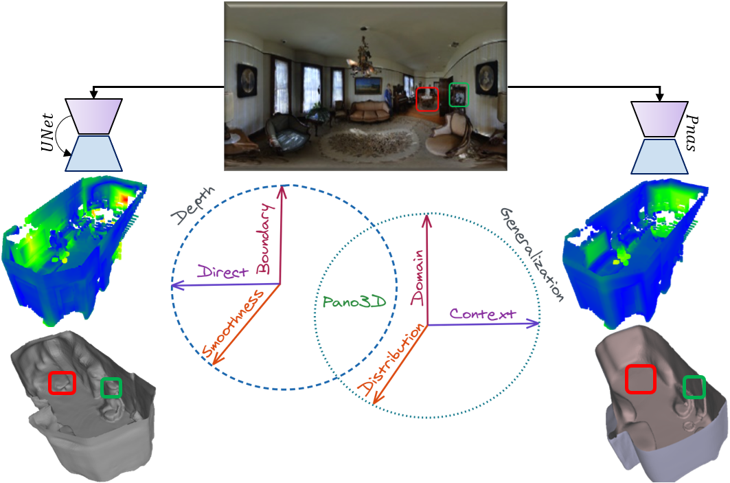
Figure 1: Preserving depth’s piece-wise smoothness should be the primary goal of data-driven depth estimation models. Yet most works only assess direct depth performance neglecting secondary traits like smoothness or boundary preservation. Different architectures (UNet – left, or Pnas – right) exhibit different inference characteristics skewed towards boundaries (UNet) or smoothness (Pnas). The Pano3D benchmark descends from a holistic perspective taking into account all performance traits, and additionally considers an orthogonal performance assessment, generalization to unseen data from different distributions, contexts or domains.

The recent availability of ${360}^{o}$ depth datasets out of stitched raw sensor data [1, 7], 3D reconstruction renderings [56, 55], and photorealistic synthetic scenes [34, 53] has stimulated research in monocular ${360}^{o}$ depth estimation [44, 13, 45, 26, 52, 43]. Still, the progress in monocular depth estimation has been mainly driven by research for traditional cameras, and assessed on perspective datasets, starting with the pioneering work of [14]. Even though other approaches exist (e.g. ordinal regression [16, 3]), depth estimation is most typically addressed as a dense regression objective. Various estimator choices are available for the direct objective like L1, L2, or robust versions like the reverse Huber (berHu) loss [32]. Complementary errors have also been introduced like the virtual normal loss [51] which captures longer range depth relations. Additional smoothness ensuring losses can be used to enforce a reasonable and established prior of depth maps, which is their piece-wise smoothly spatially varying nature [23].

Depth maps also exhibit sharp edges at object boundaries [23], whose preservation is important for various downstream applications. Recent works which focus explicitly on improving the estimated boundaries introduced new metrics to measure boundary preservation performance [21, 39]. Since convolutional data-driven methods spatially downscale the encoded representations, predicting neighboring values relies on neighborhood information, leading to interpolation blurriness. Counteracting approaches, like encoder-decoder skip connections or guided filters [47], can lead to texture transfer artifacts, hurting the predictions’ smoothness. The latter (smoothness) is also an important trait for some tasks like scene-scale 3D reconstruction which usually relies on surface orientation information [29] to preserve structural planarities, while the former (boundaries) are necessary for applications like view synthesis [2] or object retrieval [28]. Still, smoothness related metrics are usually presented on surface [46, 27] or plane [12] estimation works. Further, the balance between them needs to be tuned as they are conflicting objectives.

In this work we set to deliver an unbiased and holistic benchmark for monocular ${360}^{o}$ depth estimation that provides performance analysis across all traits, i) depth estimation, ii) boundary preservation, iii) smoothness. We also consider an orthogonal evaluation strategy that seeks to assess the models’ generalization as well, across its different facets, i) varying depth distributions, ii) adaptation to the scenes’ contexts, and iii) different camera domains. To support the benchmark, we design a set of solid baselines that respect best practises as reported in the literature and rely on standard architectures. Our results, data, code, configurations and trained models are publicly available at vcl3d.github.io/Pano3D/.

• We show that recently made available datasets contain significant biases or artifacts that prevent them from being suitable as solid benchmarks.

• We provide ${360}^{o}$ depth estimation performance results for all different traits, across different domains, contexts, distributions and resolutions, while also taking depth refinement advances into account.

• We demonstrate the effectiveness of skip connections, a rare architectural choice for (${360}^{o}$) depth estimation.

2 Related Work

Monocular Omnidirectional Depth Estimation. The first works addressing the monocular data-driven omnidirectional depth estimation task were [44] and [56]. The former applied traditional CNNs trained on perspective images in a distortion-aware manner to spherical images, while the latter introduced a rendered spherical dataset of paired color and depth images, in addition to a simplistic rectangular filtering preprocessing block. Pano Popups [12] simultaneously predict depth and surface orientation to construct planar 3D models, showing the insuffiency of depth estimates along to approximate planar regions.

The generalized Mapped Convolutions [13] were applied to omnidirectional depth estimation, showing how accounting for the distortion when using equirectangular projection increases performance in the image regions closer to the equator. Although these spatially imbalanced predictions are an important issue to address for ${360}^{o}$ depth estimation methods, the usual evaluation methodologies do not address this apart from [55]. The omnidirectional extension networks [9] employ a near field-of-view (NFoV) perspective depth camera to accompany the spherical one, offering a necessary, albeit not full FoV, constraint to enhance the preservation of details in the inferred depth map.

Recent omnidirectional depth estimation works diverged in two paths. One route is to exploit the nature of the spherical images within network architectures, with BiFuse [45] fusing features from a cubemap and an equirectangular representation, while UniFuse [26] shows that the fusion of cubemap features to the equirectangular ones is more effective. HoHoNet [43] adapts classical CNNs to operate on ${360}^{o}$ images by flattening the meridians to DCT coefficients, allowing for efficient dense feature reconstruction, and applying it to monocular depth estimation from spherical panoramas. Other recent works [34, 52] explore the connection between the layout and depth estimation tasks, while [15] relies on the joint optimization between depth and surface orientation estimates using a UNet model [41].

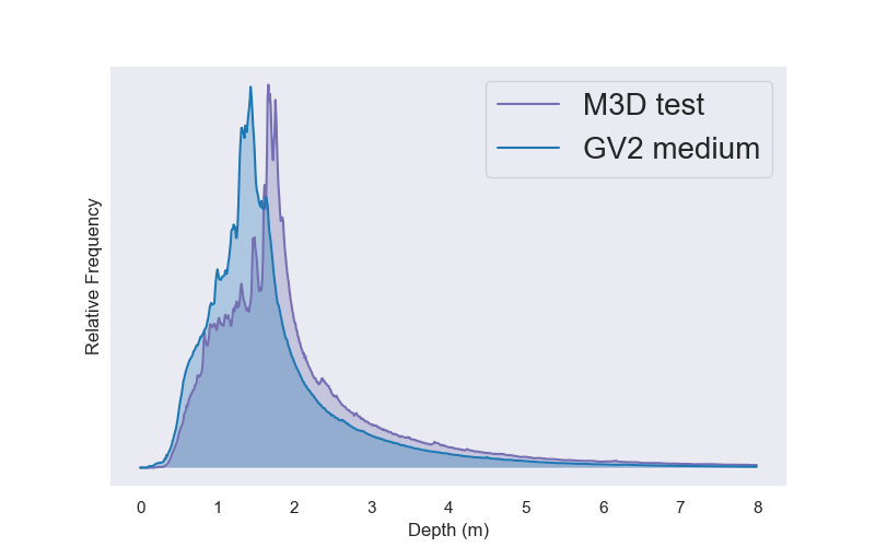
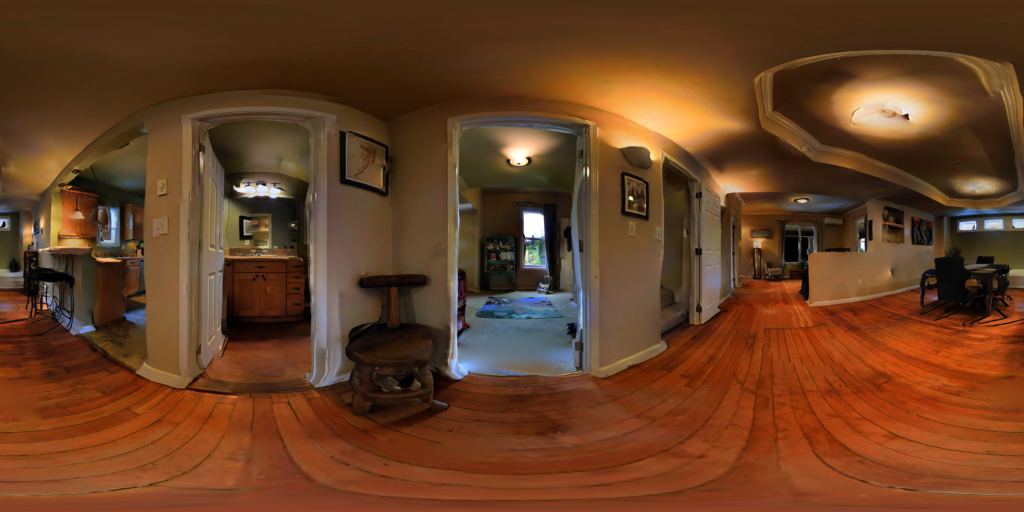
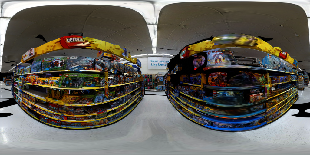
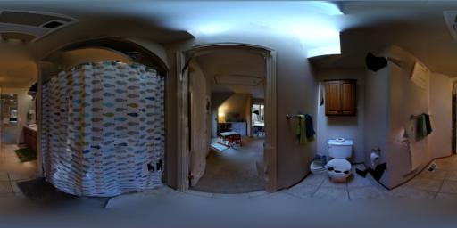
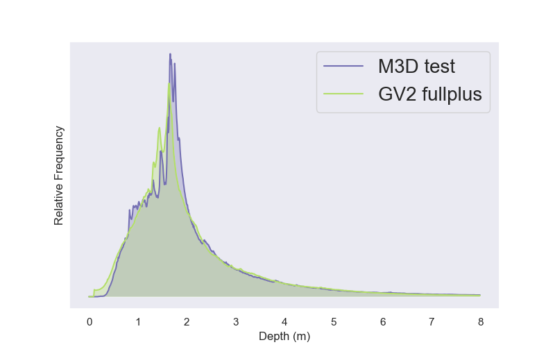
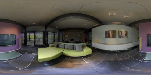
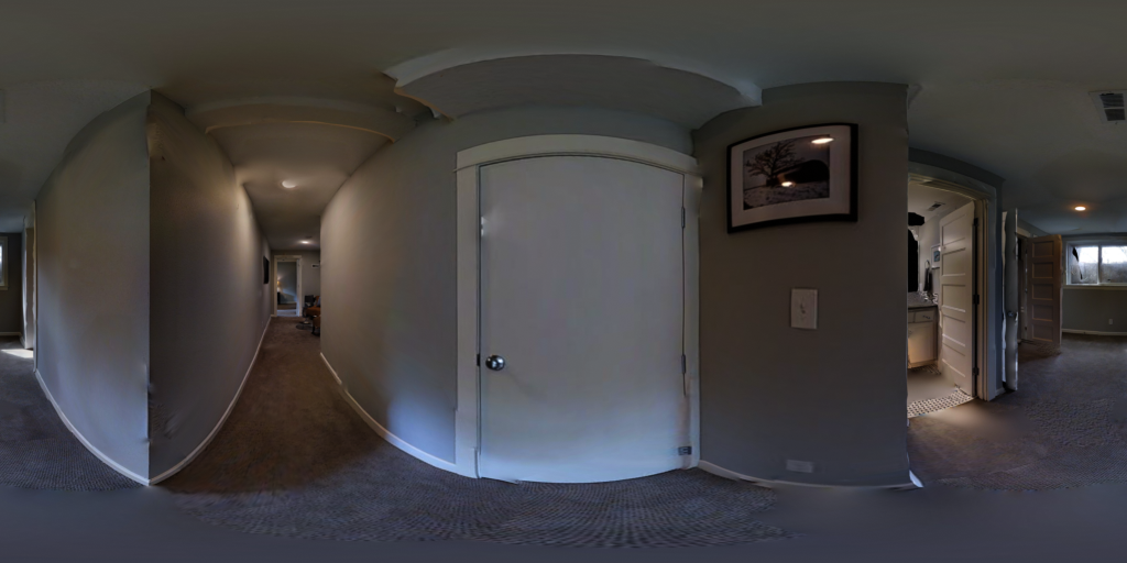
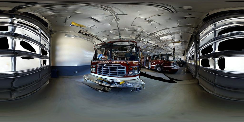
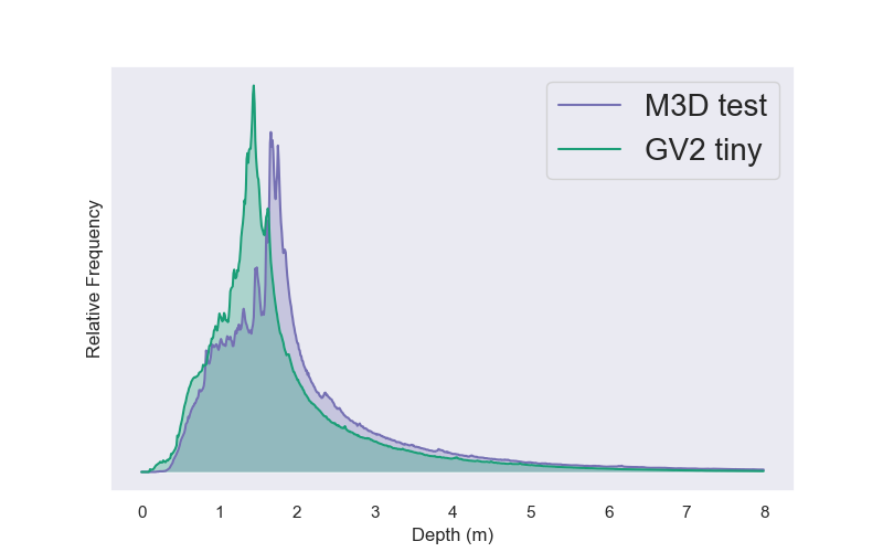
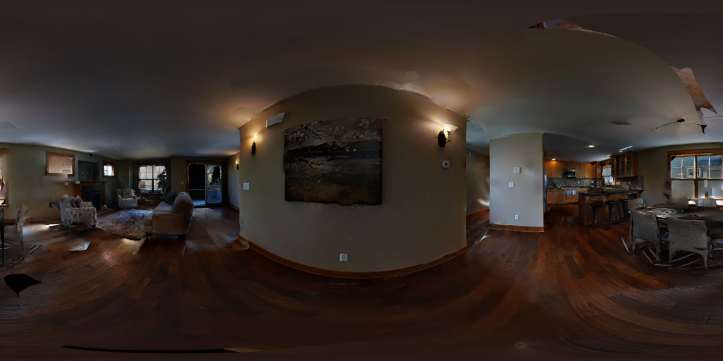
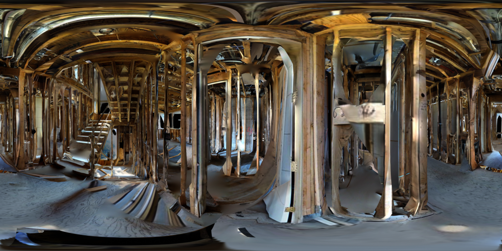
Figure 2: Existing ${360}^{o}$ depth benchmarks are either synthetic (Structured3D – tomato red) or biased (3D60, with an extra light source – orange). In addition to a holistic evaluation scheme, our benchmark Pano3D fixes the lighting issues (Matterport3D data – violet), and additionally offers a variety of zero-shot cross dataset transfer splits (generated from GibsonV2), permitting the validation of close-to-real-world performance. The tiny (dark green) and medium (dark blue) splits contain residential building scenes but with a different depth distribution as presented on the left of the figure. The fullplus (light green) split, albeit of similar distribution, contains different context scenes, like super-markers, garages and construction sites. Finally, we additionally generate camera domain adapted splits like the tiny filmic (purple) on the right, or the fullplus filmic (not shown), effectively capturing all different generalization performance traits.

Monocular Perspective Depth Estimation. The pioneering work for data-driven monocular dense depth estimation [14] employed a scale-invariant loss and established the set of metrics used to evaluate follow up works. Naturally, the progress in monocular depth estimation for perspective images is larger, as traditional images find more widespread use. While impressive gains have been presented using ordinal regression [16] or adaptive binning [3], they have not been applied to ${360}^{o}$ depth estimation, which exhibits more complex depth distributions than perspective depth maps due to its holistic FoV.

Results like the berHu loss presented in [32] have found traction in omnidirectional models as they are more easily transferable. On the contrary the more recently presented virtual normal loss [51] has not been applied to ${360}^{o}$ depth, albeit its longer range depth relation modelling is highly aligned with the global reasoning required for the spherical task. Recently, the balance between the multitude of losses required to balance smoothness, boundary preservation and depth accuracy were investigated in [33] to help models initially focus on easier to optimize losses (i.e. depth accuracy), and then on harder ones (i.e. smoothness, boundary).

Regarding depth discontinuity preservation performance, [21] showed that a combination of three different loss terms, a depth, a surface and a spatial derivative one, help increase performance at object boundaries. Similarly, a boundary consistency was introduced in [25] to overcome blurriness and bleeding artifacts. Another approach, based on learnable guided filtering [47], exploits the color image as guidance. Recently, displacement fields [39] showed that predicting resampling offsets instead of residuals is more suitable to increase performance at sharp depth discontinuities, while preserving depth estimation accuracy.

3 Methodology

Our goal is two-fold, first to deliver a new benchmark for ${360}^{o}$ depth estimation, and second, to methodically analyze the task in light of recent developments, to identify a set of solid baselines, which future works will use as the starting points for assessing performance gains. Section 3.1 introduces the benchmark data, which set the ground for the subsequent analysis. Section 3.2 describes the benchmark’s holistic approach in terms of evaluation, while Section 3.3 presents the experiment design rationale.

3.1 Dataset

Up to now ${360}^{o}$ depth datasets either rendered purely synthetic scenes like Structured3D [53] or 360D’s SunCG and SceneNet parts [56], or relied on 3D scanned datasets like Matterport3D [7] and Stanford2D3D [1]. The latter offer both panoramas and the 3D textured meshes, with some works using the original Matterport camera derived data and others the rendered panoramas from the 3D scanned meshes. Both approaches come with certain drawbacks, the original data contain invalid (i.e. true black) regions towards the sphere’s poles, while the 3D rendered data contain invalid regions where the 3D scans failed to reconstruct the surface. At the same time, the original data present with stitching artifacts (mostly blurring), while the rendered data sometimes suffer from 3D reconstruction errors which manifest in color discontinuities. We opt for the generation via rendering approach [56] as it produces true spherical panoramas and higher quality depth maps at lower resolution compared to nearest neighbor sampling. However, we fix a critical issue of the 360D [56] and 3D60 [55] datasets, namely, the introduction of a light source that alters the scene’s photorealism. Instead, we only sample the raw diffuse texture, preserving the original scene lighting, a crucial factor for unbiased learning and performance evaluation.

Zero-shot Cross-Dataset Transfer. However, there is a need to move beyond traditional train/test split performance analysis to support model deployment in real-world conditions. Thus, assessing generalization performance is very important. Towards that end, apart from re-rendering the Matterport3D scans for training, we introduce a new ${360}^{o}$ color-depth pair generated dataset from the $572$ GibsonV2 (GV2) [48] 3D scans. Compared to Matterport3D’s (M3D) $90$ buildings, it is a vastly larger dataset, whose scenes offer higher variety as well. These renders can be used for assessing generalization performance across its different splits: tiny, medium, full and fullplus. After removing outlier scans and filtering samples (keeping those with $\leq 10\%$ invalid pixels), we are left with $7170$/$1527$ train/test M3D samples, and $2740$, $6999$, $3284$, $21203$ GV2 tiny, medium, fullplus, and full split samples respectively.

Table 1: Direct depth metrics performance across models and supervision schemes. Best three performers are denoted with bold faced light green (1^st), light blue (2^nd) and light purple (3^rd) respectively following the ranking order. Same scheme applies to all tables.

Model		Depth Error $\downarrow$				Depth Accuracy $\uparrow$
		RMSE	RMSLE	AbsRel	SqRel	$\delta_{1.05}$	$\delta_{1.1}$	$\delta_{1.25}$	$\delta_{1.25^{2}}$	$\delta_{1.25^{3}}$
Pnas	$\mathcal{L}_{1}$	0.4817	0.0780	0.1213	0.0933	34.59%	59.98%	87.25%	96.30%	98.50%
	$\mathcal{L}_{cosine}$	0.4825	0.0782	0.1216	0.1014	37.04%	60.96%	87.48%	96.36%	98.46%
	$\mathcal{L}_{grad}$	0.4616	0.0749	0.1163	0.0889	37.40%	62.46%	88.39%	96.63%	98.57%
	$\mathcal{L}_{comb}$	0.4613	0.0740	0.1143	0.0892	38.56%	63.31%	88.70%	96.68%	98.62%
	$\mathcal{L}_{vnl}$	0.4640	0.0743	0.1165	0.0920	37.67%	62.60%	88.47%	96.64%	98.65%
UNet	$\mathcal{L}_{1}$	0.4215	0.2033	0.1138	0.0744	37.54%	60.47%	88.05%	97.01%	98.81%
	$\mathcal{L}_{cosine}$	0.4152	0.0841	0.1170	0.0736	34.06%	59.75%	88.13%	97.13%	98.99%
	$\mathcal{L}_{grad}$	0.4061	0.4264	0.1135	0.0682	37.49%	60.93%	88.50%	97.17%	98.91%
	$\mathcal{L}_{comb}$	0.4041	0.1459	0.1146	0.0692	37.24%	60.44%	88.31%	97.15%	99.04%
	$\mathcal{L}_{vnl}$	0.3967	0.1182	0.1095	0.0672	38.62%	62.16%	89.08%	97.35%	99.03%
DenseNet	$\mathcal{L}_{1}$	0.4672	0.5580	0.1223	0.0896	37.53%	60.52%	86.72%	96.27%	98.37%
	$\mathcal{L}_{cosine}$	0.4603	0.0752	0.1145	0.0817	37.57%	62.61%	88.03%	96.75%	98.64%
	$\mathcal{L}_{grad}$	0.4488	0.3847	0.1210	0.0827	33.25%	59.71%	87.39%	96.73%	98.63%
	$\mathcal{L}_{comb}$	0.4490	0.2565	0.1129	0.0806	38.30%	63.02%	88.56%	96.66%	98.54%
	$\mathcal{L}_{vnl}$	0.4481	0.6177	0.1142	0.0805	39.28%	63.34%	88.49%	96.66%	98.43%
ResNet	$\mathcal{L}_{1}$	0.4755	0.1639	0.1310	0.0942	31.22%	55.89%	85.56%	96.27%	98.57%
	$\mathcal{L}_{cosine}$	0.4700	0.0804	0.1279	0.0949	37.37%	57.92%	85.32%	96.35%	98.62%
	$\mathcal{L}_{grad}$	0.4734	0.2495	0.1278	0.0916	35.23%	57.34%	85.54%	96.20%	98.50%
	$\mathcal{L}_{comb}$	0.4573	0.1200	0.1272	0.0894	34.53%	57.97%	86.26%	96.56%	98.71%
	$\mathcal{L}_{vnl}$	0.4607	0.2938	0.1236	0.0862	34.75%	59.16%	86.11%	96.60%	98.60%
ResNetskip	$\mathcal{L}_{1}$	0.4373	0.2430	0.1161	0.0783	37.07%	60.60%	87.68%	96.86%	98.75%
	$\mathcal{L}_{cosine}$	0.4347	0.1070	0.1139	0.0772	39.80%	61.31%	88.27%	97.02%	98.81%
	$\mathcal{L}_{grad}$	0.4107	0.2710	0.1089	0.0717	38.93%	63.31%	89.51%	97.32%	98.92%
	$\mathcal{L}_{comb}$	0.4165	0.0843	0.1102	0.0722	36.71%	61.92%	89.17%	97.24%	98.90%
	$\mathcal{L}_{vnl}$	0.4260	0.0967	0.1125	0.0756	39.92%	62.53%	88.22%	97.04%	98.88%

3.2 Metrics

Since the introduction of the first set of metrics for data-driven depth estimation [14], namely root mean squared error (RMSE), room mean squared logarithmic error (RMSLE), absolute relative error (AbsRel), squared relative error (SqRel), and the relative threshold ($t$) based accuracies ($\delta_{t}$), these metrics are the standard approach for evaluation depth estimation performance. More recent works have identified some shortcomings of these metrics. Specifically in [31] an expanded analysis of depth estimation quality measures was conducted, and focused on two important traits, planarity and discontinuities. The latter is very important for some downstream applications like view synthesis, and apart from the completeness (comp) and accuracy (acc) of the depth boundary errors (dbe) proposed in [31], another set of accuracy metrics were proposed in [21]. The precision, recall and their harmonic mean (F1-score) were used after extracting different boundary layers via Sobel edge thresholding. Planarity is also very important for various downstream applications, especially for indoor 3D reconstruction. Finally, to overcome resolution [4] and focal length variations [8], recent perspective depth estimation works resort to nearest-neighbor 3D metrics.

Direct Depth Metrics. We build upon these developments and design our benchmark to provide a holistic evaluation of depth estimation models. Given the progress of recent data-driven models we expand the $\delta$ accuracies with two lower thresholds, a strict at $\delta_{1.1}$, and a precise, $\delta_{1.05}$, similar to [25]. However, these metrics, when applied directly on equirectangular images, are biased by its distortion towards the poles. To remove this bias we take the spherically weighted mean (denoting with a $w$ prefix), which is standard practise for ${360}^{o}$ image/video quality assessment [50] and was also used in [55]. For the $\delta_{t}$ accuracies though, we turn to uniform sampling on the sphere using the projected vertices of a subdivided icosahedron, denoted as $\delta_{t}^{ico^{K}}$, $K$ being the icosahedron’s order.

Depth Discontinuity Metrics. We complement the direct depth performance metrics with a set of secondary metrics measuring performance at preserving the depth discontinuities, usually manifesting at object boundaries. While [31] used manual annotation and structured edge detection [11], we follow the approach of [39] that relies on automatic Canny edge detection [5]. In addition, we complement the depth boundary errors (dbe^acc and dbe^comp) with the accuracy metrics of [21] (prec_t, rec_t) using the same thresholds, $t\in\{0.25,0.5,1.0\}$, for both set of metrics.

Depth Smoothness Metrics. While the planarity metric of [31] required the manual annotation of samples, its goal is to measure the smoothness of the inferred depth with respect to dominant structures. A straightforward adaptation that alleviates annotations is the use of surface orientation metrics, which is a property directly derived from the depth measurements. Using spherical-to-Cartesian coordinates conversion the depth/radius measurements are lifted to 3D points, with the surface orientation extracted by exploiting the structured nature of images. Similar to how surface estimation methods measure performance, we use the angular RMSE (RMSE^o), and a set of accuracies $\alpha_{d^{o}}$ with pre-defined angle thresholds $d$, using those from [46] ($d\in\{11.25^{o},22.5^{o},30^{o}\}$).

Geometric Metrics. Depth estimations are typically used in downstream applications for metric-scale 3D perception. Therefore, 3D performance metrics are reasonable to assess suitability for downstream tasks. We use two different metrics that aggregate the performance of the aforementioned different depth traits, i.e. accuracy and precision, boundary preservation and smoothness. The first geometric metric is computed on the point cloud level (c2c), using a point-to-plane distance between each point and its closest correspondence with the ground truth point cloud. The point-to-plane distance jointly encodes depth correctness and smoothness, while the closest point query will penalize boundary errors. The second geometric metric is computed on the mesh level, having each point cloud (predicted and ground truth) 3D reconstructed using the Screened Poisson Surface Reconstruction [29]. We then calculate the Hausdorff distance [10] between the two meshes. Similarly, Poisson reconstruction leverages both position and surface information when generating the scene’s mesh. Through this metric we assess the capacity to represent the entire scene’s geometry with the estimated depth, an important trait for some downstream applications.

3.3 Experimental Setup

We design our experiments and search for a solid baseline taking recent developments into account.

Supervision. As shown in [6] the L1 ($\mathcal{L}_{1}$) loss exhibits the best convergence for monocular depth estimation irrespective of the model size and architecture complexity, indicating that models behaving like median estimators are more appropriate. Most recent works for ${360}^{o}$ depth estimation [45, 26, 13] use the berHu loss [32], with the exception to this rule being [43] that uses the L1 loss.

We additionally observe that these works rely solely on a single direct depth loss, while recent works on perspective depth estimation also include additional losses. MiDaS [40], MegaDepth [35] as well as [49] and [21] use a multi-scale ($K=4$ scales) gradient matching term ($\mathcal{L}_{grad}$) that enforces consistent depth discontinuities. While their terms are scale-invariant and operate in the log-space, ${360}^{o}$ depth does not suffer from disparity/baseline or focal length variations, and since we do not use the L1 loss in log-space (as its performance is inferior to pure L1 [6]), we use a non-scale invariant version of this loss. Apart from boundary preservation, the piece-wise smooth nature of depth, necessitates the use of a suitable prior for the predictions. This was acknowledged in [21], where a surface orientation consistency loss was used ($\mathcal{L}_{cosine}$). Prior works employed smoothness priors on the predictions, and, to overcome cross boundary smoothing, relied on image gradient weighting [18]. Yet image gradients do not necessarily align with depth discontinuities, making the normal loss a better candidate.

Finally, the newly introduced virtual normal loss [51] ($\mathcal{L}_{vnl}$) is a long-range relationship oriented objective, which given the global context of spherical panoramas is well aligned with the task. In our experiments we follow a progressive loss ablation starting with a $\mathcal{L}_{1}$ objective, examining the effect of $\mathcal{L}_{grad}$ and $\mathcal{L}_{cosine}$ on the $\mathcal{L}_{1}$ baseline, as well as their combined effect $\mathcal{L}_{comb}$, and finally further extend the combined objective with $\mathcal{L}_{vnl}$, with the latter experiment including all losses.

Model Architecture. The importance of high-capacity encoders, pre-training and multi-scale predictions is acknowledged in the literature [40]. Building on the first, we preserve a consistent convolution decoder and use a DenseNet-161 [22] ($55$M parameters) and ResNet-152 [20] ($110$M parameters) encoder as baselines. Inspired by recent work [33] we also include their Pnas model ($99$M parameters) whose encoder is a product of neural architecture search [36]. In addition, taking into account the boundary preservation performance of skip connections, we also use the – largely unpopular for depth estimation – UNet model [41] ($27$M parameters). Since it is a purely convolutional model, we additionally modify the ResNet-152 model with skip connections starting from the first residual block ($112$M parameters), in contrast to UNet’s very early layer encoder-to-decoder skip. Since pre-training weights are not available for UNet, we experiment with cold-started models, and also simplify training using a single-scale predictions as the multi-scale effect should be horizontal across all models with the same convolution decoder structure.

Periodic Displacement Fields Refinement. We additionally consider the refinement of the predicted depth, using a shallow hourglass module [38]. It is adapted for the task at hand, with two branches, one for the input color image and the other for the predicted depth map. Across each stage, we account for the varying nature of each branch’s feature statistics using Adaptive Instance Normalization [24]. We follow the recent approach of [39] that shows how predicting displacement fields instead of residuals produces higher quality depth refinement. However, the spherical domain is continuous, and thus, we need to account for the horizontal discontinuity of the equirectangular projection. To achieve this in a locally differentiable manner, we resort to a periodic reconstruction of the sampling coordinates. Considering the final sampling coordinates $(\phi,\theta)$ after adding the displacement field, we wrap them around to $(\tau,\theta)$, with $\tau=\operatorname{atan2}(-\sin\phi,-\cos\phi)+\pi$.

Training and Evaluation. We train all models solely on the official train split of M3D, and evaluate them on its official test split as well. Evaluation is conducted across all the aforementioned axes of depth performance. Apart from this holistic performance analysis, we additionally take an orthogonal direction and assess the models’ generalization performance on zero-shot cross-dataset transfer using the GV2 tiny, medium and fullplus splits. Given that both GV2 and M3D scenes were scanned with same type of camera (i.e. Matterport), we render another version of tiny which is tone mapped to a film-like dynamic range, dubbed tiny-filmic, changing the camera-related data domain. Our experiments are conducted on two different resolutions $512\times 256$ and $1024\times 512$ (we render all datasets to both) to assess cross-resolution performance.

Table 2: Direct depth performance using spherical metrics. A UNet model with spherical padding is also presented (light pink), as well as the two better performing models trained and tested on the 3D60 (light orange) and Structured3D (light red) datasets.

Model	Depth Error $\downarrow$				Depth Accuracy $\uparrow$
	$w$RMSE	$w$RMSLE	$w$AbsRel	$w$SqRel	$\delta_{1.05}^{ico^{6}}$	$\delta_{1.1}^{ico^{6}}$	$\delta_{1.25}^{ico^{6}}$	$\delta_{1.25^{2}}^{ico^{6}}$	$\delta_{1.25^{3}}^{ico^{6}}$
Pnas$comb$	0.5367	0.0811	0.1259	0.1153	36.44%	60.52%	86.80%	95.83%	98.11%
UNet$vnl$	0.4520	0.1300	0.1147	0.0811	36.68%	60.59%	88.31%	96.96%	98.73%
DenseNet$comb$	0.5209	0.1982	0.1209	0.1013	35.97%	60.41%	87.02%	95.96%	98.09%
ResNet$comb$	0.5294	0.1365	0.1374	0.1127	32.03%	55.31%	84.74%	95.81%	98.21%
ResNet$comb$skip	0.4788	0.0927	0.1166	0.0893	36.20%	60.64%	87.99%	96.62%	98.49%
UNet$vnl$circ	0.4399	0.0685	0.1132	0.0769	36.85%	61.38%	88.84%	97.25%	98.89%
UNet$vnl$  @ 3D60	0.3140	0.0455	0.0741	0.0316	49.99%	75.16%	95.49%	99.11%	99.60%
ResNet $comb$skip  @ 3D60	0.3758	0.6100	0.0883	0.0481	46.03%	70.29%	93.12%	98.41%	99.34%
UNet$vnl$  @ S3D	0.1815	0.0546	0.0919	0.0398	50.61%	75.98%	92.23%	96.56%	97.53%
ResNet$comb$skip  @ S3D	0.2450	0.1335	0.1349	0.1249	40.48%	67.29%	88.67%	95.01%	96.68%

Table 3: Top half: Depth discontinuity/boundary preservation and depth smoothness performance metrics. Bottom half: Same metrics after refining all models (subscript ref) with a periodic displacement field hourglass module.

Model	Depth Discontinuity								Depth Smoothness
	Error $\downarrow$		Accuracy $\uparrow$						Error $\downarrow$	Accuracy $\uparrow$
	dbeacc	dbecomp	prec$0.25$	prec$0.5$	prec$1$	rec$0.25$	rec$0.5$	rec$1$	RMSEo	$\alpha_{11.25^{o}}$	$\alpha_{22.5^{o}}$	$\alpha_{30^{o}}$
Pnas$comb$	2.5119	5.3501	39.83%	31.59%	27.01%	23.53%	14.42%	10.98%	15.26	67.73%	77.99%	81.67%
UNet$vnl$	1.2699	3.8876	58.97%	57.54%	51.85%	43.96%	36.69%	28.59%	16.02	61.80%	76.58%	81.70%
DenseNet$comb$	2.0628	5.0977	47.16%	40.77%	35.20%	26.09%	16.87%	12.21%	15.98	64.58%	76.86%	81.20%
ResNet$comb$	2.2393	5.3796	44.10%	36.70%	27.44%	22.91%	12.23%	7.20%	16.63	63.09%	75.70%	80.20%
ResNet$comb$skip	1.4883	4.5346	57.34%	54.11%	47.57%	33.99%	24.30%	16.37%	15.27	64.18%	77.57%	82.27%
Pnas$comb$ref	2.2861	5.0435	46.66%	44.74%	37.96%	30.66%	26.00%	22.49%	17.83	63.33%	74.01%	78.15%
UNet$vnl$ref	1.4241	3.8505	53.46%	51.38%	44.36%	43.09%	41.54%	37.50%	16.86	61.50%	75.70%	80.64%
DenseNet$comb$ref	1.9769	4.9026	51.94%	48.43%	40.63%	30.61%	26.14%	22.46%	16.49	63.80%	76.17%	80.58%
ResNet$comb$ref	2.1078	5.0783	50.77%	46.52%	36.58%	28.31%	23.33%	19.37%	16.68	63.08%	75.82%	80.36%
ResNet$comb$skip & ref	1.4291	4.3115	60.78%	58.09%	51.49%	37.79%	32.55%	27.23%	15.05	65.16%	78.26%	82.77%

Table 4: Consolidated performance on the GibsonV2 splits, across all depth traits, using a subset of the available metrics, for models trained on the Matterport3D data. The best performing model (UNet) trained with photometric augmentation is also presented (light pink).

GV2	Model	Direct Depth					Depth Discontinuity					Depth Smoothness
		Error $\downarrow$			Accuracy $\uparrow$		Error $\downarrow$		Accuracy $\uparrow$			Error $\downarrow$	Accuracy $\uparrow$
		$w$RMSE	$w$RMSLE	$w$AbsRel	$\delta_{1.1}^{ico^{6}}$	$\delta_{1.25}^{ico^{6}}$	dbeacc	dbecomp	prec$0.25$	prec$0.5$	prec$1$	RMSEo	$\alpha_{30^{o}}$
tiny	Pnas$comb$	0.5574	0.0970	0.1945	36.01%	76.76%	2.6616	5.6187	34.90%	30.67%	25.07%	15.91	81.68%
	UNet$vnl$	0.4723	0.2060	0.1733	41.67%	81.49%	1.4726	4.3377	61.43%	64.51%	60.21%	17.35	80.71%
	DenseNet$comb$	0.5131	0.1368	0.1738	38.62%	79.99%	2.2068	5.2911	43.19%	40.05%	35.32%	16.24	81.66%
	ResNet$comb$	0.5426	0.1427	0.2113	31.87%	72.80%	2.3665	5.5963	40.64%	37.11%	30.21%	16.97	80.64%
	ResNet$comb$skip	0.4932	0.0900	0.1747	39.26%	79.86%	1.6406	4.7710	55.44%	56.69%	52.48%	16.24	81.93%
	UNet$vnl$skip & aug	0.4580	0.0840	0.1701	39.73%	81.19%	1.4480	4.2681	62.69%	66.19%	62.27%	16.30	82.16%
medium	Pnas$comb$	0.5053	0.0926	0.1866	34.85%	78.58%	2.6420	5.5068	36.54%	31.80%	27.25%	14.31	84.06%
	UNet$vnl$	0.4416	0.1876	0.1665	42.49%	82.50%	1.5245	4.3178	62.75%	65.68%	60.22%	16.39	82.43%
	DenseNet$comb$	0.4661	0.1670	0.1669	39.30%	81.72%	2.2311	5.2215	44.53%	41.16%	36.07%	15.15	83.50%
	ResNet$comb$	0.5023	0.1317	0.2058	32.12%	73.67%	2.3915	5.4622	41.86%	37.73%	30.38%	15.86	82.48%
	ResNet$comb$skip	0.4563	0.0884	0.1677	39.98%	81.34%	1.6930	4.7230	56.33%	57.24%	51.81%	15.44	83.30%
	UNet$vnl$skip & aug	0.4321	0.0823	0.1673	39.70%	81.90%	1.5045	4.2659	63.94%	67.27%	61.69%	15.43	83.70%
fullplus	Pnas$comb$	0.6759	0.1139	0.1991	38.60%	73.75%	2.8383	6.1612	32.61%	26.83%	21.81%	19.83	75.93%
	UNet$vnl$	0.6167	0.2657	0.1844	42.42%	76.21%	1.7228	5.0369	54.45%	56.37%	52.31%	22.05	73.41%
	DenseNet$comb$	0.6684	0.1649	0.1835	40.79%	74.87%	2.4985	6.0993	39.33%	34.44%	27.63%	20.57	75.18%
	ResNet$comb$	0.6690	0.1504	0.2095	37.35%	71.42%	2.6259	6.2642	37.82%	32.27%	23.59%	21.00	74.54%
	ResNet$comb$skip	0.6370	0.1183	0.1828	41.28%	75.45%	1.9257	5.5758	50.05%	48.96%	41.74%	20.61	75.18%
	UNet$vnl$skip & aug	0.6014	0.1033	0.1758	42.70%	76.97%	1.7040	5.0063	56.24%	58.18%	53.33%	20.87	75.09%
tiny filmic	Pnas$comb$	0.6268	0.1088	0.1939	37.03%	75.66%	2.9347	6.1523	32.01%	27.16%	21.20%	17.34	79.73%
	UNet$vnl$	0.5448	0.2315	0.1848	42.82%	79.43%	1.6943	4.8443	57.63%	59.49%	53.19%	19.21	78.00%
	DenseNet$comb$	0.6903	0.1896	0.1968	35.34%	73.48%	2.8225	6.3933	37.14%	31.85%	24.24%	19.29	77.37%
	ResNet$comb$	0.6107	0.1479	0.2036	35.08%	73.29%	2.7016	6.1781	37.34%	32.57%	22.22%	18.30	78.64%
	ResNet$comb$skip	0.6445	0.1195	0.1863	39.00%	75.19%	2.1093	5.7670	50.19%	48.58%	37.50%	19.26	77.35%
	UNet$vnl$skip & aug	0.4750	0.0871	0.1743	39.51%	80.39%	1.5326	4.3923	60.69%	63.32%	59.43%	16.66	81.62%
fullplus filmic	Pnas$comb$	0.7866	0.1344	0.2129	35.97%	68.86%	3.1505	6.7791	29.06%	22.40%	16.16%	21.55	73.61%
	UNet$vnl$	0.7368	0.2975	0.2199	38.47%	70.20%	1.9476	5.5601	50.65%	50.90%	44.46%	23.89	70.69%
	DenseNet$comb$	0.9258	0.2207	0.2292	33.54%	63.80%	3.1514	7.1900	32.52%	25.41%	17.75%	24.04	70.14%
	ResNet$comb$	0.7786	0.1727	0.2154	35.99%	68.24%	2.9668	6.8743	34.37%	27.06%	16.76%	22.50	72.35%
	ResNet$comb$skip	0.8705	0.1632	0.2217	34.94%	65.30%	2.4696	6.6184	43.73%	39.23%	27.65%	23.91	70.13%
	UNet$vnl$skip & aug	0.6237	0.1084	0.1829	41.57%	75.56%	1.7688	5.1482	54.64%	55.56%	50.02%	21.23	74.58%

Table 5: Consolidated depth performance across all traits using a subset of the available metrics. Results are presented for the two best performing models on the GibsonV2 splits which have been trained on the Matterport3D train split.

GV2	Model	Direct Depth					Depth Discontinuity					Depth Smoothness
		Error $\downarrow$			Accuracy $\uparrow$		Error $\downarrow$		Accuracy $\uparrow$			Error $\downarrow$	Accuracy $\uparrow$
		$w$RMSE	$w$RMSLE	$w$AbsRel	$\delta_{1.1}^{ico^{6}}$	$\delta_{1.25}^{ico^{6}}$	dbeacc	dbecomp	prec$0.25$	prec$0.5$	prec$1$	RMSEo	$\alpha_{30^{o}}$
tinyHR	UNet$vnl$	0.5794	0.1247	0.2151	31.98%	62.05%	1.4330	5.1737	44.84%	46.13%	41.57%	22.36	74.12%
	ResNet$comb$skip	0.4993	0.1273	0.1758	40.78%	80.31%	1.9271	5.9666	36.24%	37.68%	30.77%	15.65	82.78%
mediumHR	UNet$vnl$	0.5901	0.1291	0.2269	31.21%	61.02%	1.6221	5.5436	43.98%	44.21%	38.46%	22.13	74.73%
	ResNet$comb$skip	0.4528	0.1618	0.1664	42.03%	81.91%	2.0356	5.8467	34.27%	34.60%	27.81%	14.71	84.46%
fullplusHR	UNet$vnl$	0.8772	0.1769	0.2730	22.46%	46.09%	1.7532	6.4628	36.46%	35.80%	28.67%	27.43	65.07%
	ResNet$comb$skip	0.6607	0.2308	0.1836	41.18%	74.77%	2.3775	6.9102	28.70%	28.15%	20.71%	19.88	76.30%

4 Analysis

Implementation Details. We implement all experiments with moai [37], using the same seed across all experiments. For data generation we use Blender and the Cycles path tracer using $256$ samples. Our ResNets are built with pre-activated bottleneck blocks [20] and all our models’ weights are initialized with [19]. We optimize all models for $60$ epochs on a NVidia 2080 Ti, using Adam [30] with a learning rate of $0.0002$ and default momentum parameters, and a consistent batch size of $4$. All losses are unity (i.e. equally) weighted across all experiments. We use CloudCompare to calculate the c2c distance [17], and MeshLab to calculate the m2m distance [10]. During evaluation, we consider the raw values predicted by the models and clip the valid depth range to $10$m.

Which loss combination offers better performance? Contrary to their focused nature both $\mathcal{L}_{cosine}$ and $\mathcal{L}_{grad}$ increase depth estimation performance across all models when complementing the direct $\mathcal{L}_{1}$ objective, as evident in Table 1. In addition, they provide the expected boost in smoothness/discontinuity preservation across all models as presented in our supplementary material which is appended after the references. When viewed purely from a depth estimation perspective, it is observed that their combination, $\mathcal{L}_{comb}$, benefits performance. But, when examining the specific depth traits that they seek to enforce, their conflicting nature is also apparent. Overall, we observe almost all models achieve highest overall performance when both losses are present, with, our without the virtuan normal loss (VNL) which is added in the $\mathcal{L}_{vnl}$ case. The latter greatly boosts the UNet model, which is reasonable as the localised nature of skip connections is aided by the global depth constraints that VNL introduces.

Which architecture is better performing? We compare architectures after selecting the best performing models for each, which for UNet is $\mathcal{L}_{vnl}$, and for the rest the $\mathcal{L}_{comb}$. The rationale for choosing $\mathcal{L}_{comb}$ for ResNet_skip is that while $\mathcal{L}_{grad}$ behaves better on direct depth metrics (except closer distances, as indicated by the RMSLE), there is a large performance gap in the discontinuity and smoothness metrics, compared to the performance discrepancy on depth estimation. Table 2 presents the results using the spherical metrics that account for the distortion. These are unbiased metrics, which is evident given the deteriorated performance across all metrics compared to those estimated on the image level on each equirectangular panorama. A more straightforward comparison is available in our supplementary material appended after the references. Interestingly, we observe that models employing encoder-decoder skip connections exhibit better performance both in direct depth metrics (Table 2). Curiously, contrary to the expectation as set by the literature [40] that high-capacity encoders are required, the UNet architecture showcases the best performance. Regarding domain oriented techniques, we train the better performing model with circular padding [42, 54] that connects features across the horizontal equirectangular boundary, denoted as circ. Evidently, this simple scheme increases the performance across all metrics, allowing the model to exploit its spherical nature.

Is this performance consistent when considering secondary traits? Regarding the discontinuity and smoothness traits as presented in Table 3 it is evident that skip connections result in higher performance, but especially for the dominating UNet, at the expense of the smoothness trait. This is reasonable as early layer skip connections result into texture transfer, and further evidenced by the improved performance of ResNet_skip, which lacks early layer skips, on both discontinuity and smoothness metrics. Overall, UNet achieves the best performance on depth and discontinuity metrics at the expense of the smoothness trait and closer range performance as indicated by its inferior RMSLE. On the other side, the different metrics indicate that the PNAS model produces oversmoothed results that are more metrically accurate and precise at closer distances. Nonetheless, ResNet_skip achieves a better balance without significant sacrifices across the secondary traits.

How helpful is depth refinement? We also examine the effect of a shallow depth refinement module on these models, with the results after training for $10$ epochs presented in Table 3. All models, apart from UNet, improve their performance at boundary preservation while also preserving depth estimation performance, but at the expense of smoothness, with the exception in this case being ResNet_skip. For UNet specifically, texture transfer leads to noise, which prevents an interpolation-based warping technique to improve results, as it was designed to improve smooth depth predictions. However, ResNet_skip closes the performance gap and even improves smoothness performance, further solidifying its well-balanced nature.

Why this benchmark? Table 2 shows the performance of the two higher performing models when trained and tested on other recently introduced ${360}^{o}$ depth datasets, namely 3D60 [55] which is an extension of [56] and Structured3D [53] with $512\times 256$ and $1024\times 512$ resolutions respectively. All metrics are significantly higher which evidences their insuitability to be used for benchmarking progress. This is largely because of their inherent bias which is the result of lighting for 3D60, which includes an extra light source at the center, as also explained in [26], an unfortunate bias that models learn to exploit as farther depths are darker; and the omission of the noisy camera-based image formation process and lack of real-world scene complexity exhibited by the purely synthetic Structure3D dataset,

What is their generalization capacity? We test these models in a zero-shot cross-dataset transfer setting using the GV2 splits using a subset of all metrics with the results presented in Table 4. We observe reduced performance for all models across all splits which is the result applying these models in different contexts/scenes and to out-of-distribution depths (tiny/medium). Yet, the ranking between models is not severely disrupted, indicating that architecture changes do not significantly affect generalization. The fullplus split is noticeably harder than the others, as all metrics are considerably worse, showcasing that pure context shifts (similar depth distribution) are detrimental to performance. However, camera domain shifts are another generalization barrier that is significant, as shown by the models’ results on the filmic splits, where a different color transfer function was applied during rendering. The latter also received the bigger gains when training with photometric augmentation (UNet_aug), specifically random gamma, contrast, brightness and saturation shifts, which also boosted performance horizontally across all splits. Still, augmentation alone did not raise performance to levels similar to the M3D test set, indicating that other techniques are required.

Table 6: Performance of all models using the 3D metrics. For the m2m metric inside the parentheses, we also report the percentage (%) of the error w.r.t the bounding box diagonal, while for the c2c metric we also report the error standard deviation.

model	m2m	c2c
Pnas$comb$	0.2502 (7.02%)	0.1439 (0.1881)
UNet$vnl$	0.2397 (6.52%)	0.1305 (0.1663)
DenseNet$comb$	0.2475 (6.98%)	0.1425 (0.1852)
ResNet$comb$	0.2573 (7.01%)	0.1405 (0.1907)
ResNet$comb$skip	0.2424 (6.83%)	0.1300 (0.1770)

How does performance vary with resolution? Given their ${360}^{o}$ FoV, spherical panoramas require higher resolutions to be able to more robustly estimate detailed depth. Table 5 presents the results of the two better performing models, trained on M3D’s $1024\times 512$ resolution data, and tested on the GV2 splits with the same resolution. We observe a change in performance between the UNet and the ResNet with skip connections. The latter’s expanded receptive field and higher capacity encoder offer significantly higher performance in the direct depth and smoothness metrics, albeit the UNet still localizes boundaries better.

How about downstream application suitability? We also assess each model’s performance using the 3D metrics that aggregate performance across all axes. Table 6 presents the results using the cloud and mesh distances are presented in Section 3.2. Overall the performance ranking is preserved, with UNet’s noisy predictions being moderated by the reconstruction process in the mesh distance metric, while the point cloud distance’s nearest-neighbor nature is more sensitive to it. Thus, downstream applications like view synthesis should investigate model results using c2c metrics, while applications relying on 3D reconstruction should resort to the m2m metric. Again, as shown by these metrics, the skip connections based ResNet is a reasonably balanced choice, that follows UNet’s top performance.

5 Summary

Spherical depth estimation is a task that comes with certain advantages (holistic view) and disadvantages (resolution requirements) compared to traditional – perspective – depth estimation. Preserving boundaries is challenging because of the distortion frequently squeezing objects towards the equator, and thus, smaller spatial areas; and due to the discontinuities that the different projections introduce. Imposing a smoothness prior is also not straightforward as for perspective depth. The presented Pano3D benchmark can stimulate future progress in ${360}^{o}$ depth estimation that will take all these aspects into account. From our extensive analysis – which nonetheless does not cover all cases – we identify the effectiveness of skip connections in terms of boundary preservation, as a means to overcome the weakness of spatial downscaling, which in turn, is necessary to exploit the panoramas’ global context. While the UNet architecture achieves top performance in lower resolutions, a ResNet with skip connections is a more balanced architectural choice that scales better across resolutions.

Finally, Pano3D relies on zero-shot cross-dataset transfer to move beyond a simple train/test split performance comparison. By decomposing generalization into three distinct performance reducing barriers, our goal is better facilitate the assessment towards real-world applicability of data-driven models for ${360}^{o}$ geometric inference.

Supplementary Material.

We provide extra quantitative and qualitative comparisons in the supplementary material following the references. Supplementing experiments also reproduce prior work used as a basis for designing our methodology. Finally, a live web demo of our baseline models can be found at share.streamlit.io/tzole1155/ThreeDit.

Appendix A Supplementary Material

This supplementary material complements our original manuscript with additional quantitative results, offering extra ablation experiments, providing qualitative results on real data and comparisons between the different architectures.

A.1 Quantitative Results

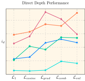
(a)

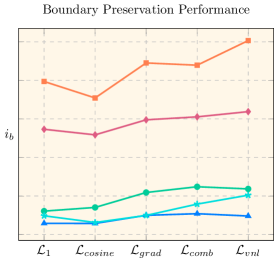
(b)

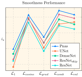
(c)

Figure 3: Performance indicators (higher is better) of different loss functions per model in three different axis. From left to right: depth indicator $i_{d}$, boundary indicator $i_{b}$ and smoothness indicator $i_{s}$.

Table 7 complements Table 1 of the main document, presenting the performance of all remaining metrics, namely the spherical direct depth metrics, the boundary preservation metrics, and the smoothness metrics. In addition, Figure 3 presents the different models’ performance in terms of three indicators, one for each trait. These indicators combine an error and an accuracy metric:

$$i_{d} =\frac{1}{(1-\delta_{1.25})\times RMSE},$$ (1)

$$i_{b} =\frac{1}{(1-\nicefrac{{(F_{0.25}+F_{0.5}+F_{1.0})}}{{3}})\times dbe^{acc}},$$ (2)

$$i_{s} =\frac{1}{(1-\nicefrac{{(\alpha_{11.25^{o}}+\alpha_{22.5^{o}}+\alpha_{30^{o}})}}{{3}})\times RMSE^{o}},$$ (3)

with $i_{d},i_{b},$ and $i_{s}$ the depth, boundary and smoothness performance indicators. Evidently, UNet performs significantly better than the other models, especially in the boundary consistency metrics, while all models benefit of the addition of extra losses. The addition, of skip connections in a common ResNet architecture offers better performance. While $\mathcal{L}_{grad}$ offers better depth performance for ResNet_skip, the variant trained with $\mathcal{L}_{comb}$ offers higher performance across the two secondary traits.

In addition, we complement the main’s paper spherical metrics Table 8 by collating the traditional ones for a straightforward comparison.

Table 7: Three axis depth metrics performance across models and supervision schemes. Best three performers are denoted with bold faced light green (1^st), light blue (2^nd) and light purple (3^rd) respectively following the ranking order. Same scheme applies to all tables.

Model		Direct Depth									Depth Discontinuity								Depth Smoothness
		Error $\downarrow$				Accuracy $\uparrow$					Error $\downarrow$		Accuracy $\uparrow$						Error $\downarrow$	Accuracy $\uparrow$
		$w$RMSE	$w$RMSLE	$w$AbsRel	$w$SqRel	$\delta_{1.05}^{ico^{6}}$	$\delta_{1.1}^{ico^{6}}$	$\delta_{1.25}^{ico^{6}}$	$\delta_{1.25^{2}}^{ico^{6}}$	$\delta_{1.25^{3}}^{ico^{6}}$	dbeacc	dbecomp	prec$0.25$	prec$0.5$	prec$1$	rec$0.25$	rec$0.5$	rec$1$	RMSEo	$\alpha_{11.25^{o}}$	$\alpha_{22.5^{o}}$	$\alpha_{30^{o}}$
Pnas	$\mathcal{L}_{1}$	0.5606	0.0854	0.1328	0.1196	32.69%	56.94%	85.12%	95.38%	97.95%	2.6542	5.7303	38.73%	30.26%	23.58%	18.74%	10.48%	8.48%	20.12	53.88%	69.81%	75.65%
	$\mathcal{L}_{cosine}$	0.5622	0.0858	0.1338	0.1317	34.49%	58.06%	85.52%	95.44%	97.88%	2.7194	5.4964	36.16%	27.76%	22.22%	21.48%	13.55%	10.02%	15.70	67.14%	77.37%	81.05%
	$\mathcal{L}_{grad}$	0.5374	0.0822	0.1276	0.1146	35.68%	59.54%	86.41%	95.72%	98.04%	2.5008	5.4548	40.91%	32.05%	25.27%	22.49%	12.17%	9.07%	18.12	59.56%	73.24%	78.30%
	$\mathcal{L}_{comb}$	0.5367	0.0811	0.1259	0.1153	36.44%	60.52%	86.80%	95.83%	98.11%	2.5119	5.3501	39.83%	31.59%	27.01%	23.53%	14.42%	10.98%	15.26	67.73%	77.99%	81.67%
	$\mathcal{L}_{vnl}$	0.5403	0.0815	0.1280	0.1183	35.43%	59.72%	86.58%	95.79%	98.11%	2.5141	5.3893	40.14%	31.77%	24.47%	22.14%	12.69%	8.74%	15.57	66.61%	77.34%	81.23%
UNet	$\mathcal{L}_{1}$	0.4834	0.2361	0.1211	0.0913	35.18%	58.24%	86.80%	96.45%	98.43%	1.4011	4.3152	57.59%	58.00%	53.85%	38.74%	31.57%	24.31%	24.66	36.80%	60.60%	69.73%
	$\mathcal{L}_{cosine}$	0.4736	0.0906	0.1217	0.0891	32.65%	58.04%	87.40%	96.68%	98.61%	1.4513	5.0455	55.35%	52.16%	46.01%	39.36%	30.01%	21.69%	15.80	63.10%	77.60%	82.38%
	$\mathcal{L}_{grad}$	0.4659	0.5186	0.1209	0.0833	35.25%	58.79%	87.33%	96.56%	98.45%	1.3305	4.0582	63.27%	63.13%	56.54%	40.39%	32.47%	23.37%	19.52	52.23%	70.40%	76.91%
	$\mathcal{L}_{comb}$	0.4630	0.1690	0.1222	0.0847	34.79%	58.21%	87.08%	96.63%	98.66%	1.3077	4.2080	63.31%	61.74%	54.96%	39.38%	30.27%	22.00%	16.19	61.01%	76.18%	81.45%
	$\mathcal{L}_{vnl}$	0.4520	0.1300	0.1147	0.0811	36.68%	60.59%	88.31%	96.96%	98.73%	1.2699	3.8876	58.97%	57.54%	51.85%	43.96%	36.69%	28.59%	16.02	61.80%	76.58%	81.70%
DenseNet	$\mathcal{L}_{1}$	0.5441	0.6872	0.1348	0.1144	34.34%	57.10%	84.73%	95.28%	97.69%	2.3690	5.5135	40.40%	36.07%	28.78%	20.45%	11.54%	8.05%	21.08	49.98%	68.29%	74.78%
	$\mathcal{L}_{cosine}$	0.5361	0.0822	0.1239	0.1034	34.98%	59.34%	86.36%	95.94%	98.13%	2.3486	5.3702	41.01%	35.45%	29.10%	22.80%	14.19%	9.39%	15.97	64.92%	76.91%	81.15%
	$\mathcal{L}_{grad}$	0.5202	0.4655	0.1304	0.1045	32.68%	57.59%	85.69%	95.85%	98.06%	2.0789	5.2159	47.01%	40.61%	33.32%	23.68%	13.71%	9.35%	18.90	56.86%	71.79%	77.23%
	$\mathcal{L}_{comb}$	0.5209	0.1982	0.1209	0.1013	35.97%	60.41%	87.02%	95.96%	98.09%	2.0628	5.0977	47.16%	40.77%	35.20%	26.09%	16.87%	12.21%	15.98	64.58%	76.86%	81.20%
	$\mathcal{L}_{vnl}$	0.5232	0.7560	0.1258	0.1030	36.28%	60.04%	86.61%	95.66%	97.74%	2.0525	5.0931	44.81%	40.14%	32.30%	25.21%	15.71%	10.33%	16.51	63.43%	76.02%	80.53%
ResNet	$\mathcal{L}_{1}$	0.5500	0.1922	0.1394	0.1186	30.59%	54.17%	84.07%	95.47%	98.03%	2.4386	5.7688	39.10%	31.69%	23.28%	20.92%	10.24%	6.32%	22.83	44.68%	64.51%	72.02%
	$\mathcal{L}_{cosine}$	0.5435	0.0864	0.1364	0.1194	34.77%	56.32%	84.29%	95.64%	98.11%	2.6918	5.7928	38.35%	32.13%	26.82%	21.88%	12.61%	8.71%	16.37	64.24%	76.30%	80.63%
	$\mathcal{L}_{grad}$	0.5475	0.2976	0.1387	0.1151	32.43%	54.46%	83.76%	95.37%	97.97%	2.4112	5.7959	41.87%	33.23%	21.60%	21.31%	9.27%	4.95%	20.50	52.77%	68.97%	75.00%
	$\mathcal{L}_{comb}$	0.5294	0.1365	0.1374	0.1127	32.03%	55.31%	84.74%	95.81%	98.21%	2.2393	5.3796	44.10%	36.70%	27.44%	22.91%	12.23%	7.20%	16.63	63.09%	75.70%	80.20%
	$\mathcal{L}_{vnl}$	0.5324	0.3320	0.1301	0.1070	33.60%	57.50%	85.20%	95.83%	98.07%	2.1335	5.1866	45.00%	38.70%	30.85%	24.88%	14.43%	9.28%	17.07	61.99%	75.22%	79.91%
ResNetskip	$\mathcal{L}_{1}$	0.5041	0.2924	0.1259	0.0977	34.10%	57.64%	86.05%	96.13%	98.30%	1.5462	4.7640	49.48%	47.23%	43.31%	32.86%	23.57%	16.63%	22.30	44.07%	65.82%	73.55%
	$\mathcal{L}_{cosine}$	0.5024	0.1207	0.1208	0.0958	37.15%	59.61%	87.03%	96.34%	98.35%	1.6012	4.7078	52.83%	49.23%	41.05%	32.03%	23.82%	16.75%	15.76	63.32%	77.05%	81.83%
	$\mathcal{L}_{grad}$	0.4754	0.3274	0.1183	0.0905	36.23%	60.44%	87.96%	96.62%	98.45%	1.5013	4.4831	56.27%	54.26%	47.88%	33.96%	23.52%	16.07%	18.72	55.00%	71.76%	77.82%
	$\mathcal{L}_{comb}$	0.4788	0.0927	0.1166	0.0893	36.20%	60.64%	87.99%	96.62%	98.49%	1.4883	4.5346	57.34%	54.11%	47.57%	33.99%	24.30%	16.37%	15.27	64.18%	77.57%	82.27%
	$\mathcal{L}_{vnl}$	0.4923	0.1095	0.1197	0.0941	37.55%	60.43%	87.23%	96.42%	98.46%	1.4629	4.1408	54.99%	51.98%	45.40%	35.29%	25.22%	17.68%	15.67	63.28%	77.05%	81.94%

Table 8: Direct depth performance using spherical and conventional metrics. Bottom part results are the same as those presented in Table 2 of the original document. Top part are the corresponding results from Table 1 of the original manuscript.

Model	Depth Error $\downarrow$				Depth Accuracy $\uparrow$
	RMSE	RMSLE	AbsRel	SqRel	$\delta_{1.05}$	$\delta_{1.1}$	$\delta_{1.25}$	$\delta_{1.25^{2}}$	$\delta_{1.25^{3}}$
Pnas$comb$	0.4613	0.0740	0.1143	0.0892	38.56%	63.31%	88.70%	96.68%	98.62%
UNet$vnl$	0.3967	0.1182	0.1095	0.0672	38.62%	62.16%	89.08%	97.35%	99.03%
DenseNet$comb$	0.4490	0.2565	0.1129	0.0806	38.30%	63.02%	88.56%	96.66%	98.54%
ResNet$comb$	0.4573	0.1200	0.1272	0.0894	34.53%	57.97%	86.26%	96.56%	98.71%
ResNet$comb$skip	0.4165	0.0843	0.1102	0.0722	36.71%	61.92%	89.17%	97.24%	98.90%
	$w$RMSE	$w$RMSLE	$w$AbsRel	$w$SqRel	$\delta_{1.05}^{ico^{6}}$	$\delta_{1.1}^{ico^{6}}$	$\delta_{1.25}^{ico^{6}}$	$\delta_{1.25^{2}}^{ico^{6}}$	$\delta_{1.25^{3}}^{ico^{6}}$
Pnas$comb$	0.5367	0.0811	0.1259	0.1153	36.44%	60.52%	86.80%	95.83%	98.11%
UNet$vnl$	0.4520	0.1300	0.1147	0.0811	36.68%	60.59%	88.31%	96.96%	98.73%
DenseNet$comb$	0.5209	0.1982	0.1209	0.1013	35.97%	60.41%	87.02%	95.96%	98.09%
ResNet$comb$	0.5294	0.1365	0.1374	0.1127	32.03%	55.31%	84.74%	95.81%	98.21%
ResNet$comb$skip	0.4788	0.0927	0.1166	0.0893	36.20%	60.64%	87.99%	96.62%	98.49%

Table 9: Direct depth performance metrics across different variations of DenseNet and Pnas.

			Depth Error $\downarrow$				Depth Accuracy $\uparrow$
model	pretrained	$\mathcal{L}$	RMSE	RMSLE	AbsRel	SqRel	$\delta_{1.25}$
DenseNet	✗	$\mathcal{L}_{1}$	0.4672	0.5580	0.1223	0.0896	86.72%
	✓	$\mathcal{L}_{1}$	0.4072	0.3194	0.1140	0.0694	88.91%
	✓	$\mathcal{L}_{log}$	0.5597	0.5720	0.1528	0.4475	80.48%
	✓	$\mathcal{L}_{berHu}$	0.4532	0.3754	0.1228	0.0852	86.68%
Pnas	✗	$\mathcal{L}_{1}$	0.4817	0.0780	0.1213	0.0933	87.25%
	✓	$\mathcal{L}_{1}$	0.3998	0.0634	0.0975	0.0661	91.91%
	✓	$\mathcal{L}_{log}$	0.4135	0.0656	0.0999	0.0697	91.09%
	✓	$\mathcal{L}_{berHu}$	0.4059	0.0643	0.0992	0.0666	91.56%

Finally, Table 9 reproduces the grounds upon our methodology was designed, namely the efficacy of pre-trained models [40] and the L1 loss [6]. We use the DenseNet and Pnas models with the encoders initialized using weights pre-trained on ImageNet. Both claims stand, with all pre-trained models achieving better performance than the model trained from scratch. In addition, the L1 loss outperforms both berHu [32] and log loss. Interestingly, the performance drops significantly in DenseNet when trained with other losses, while for Pnas the performance gap is smaller. Therefore, when benchmarking different models, this needs to be taken into account as well. Only through consistent experimentation across different aspects measurable and explainable progress will be possible.

A.2 Qualitative Results

Finally we present additional qualitative results for different models. Apart from the collation of the predicted depth maps between the different models, we provide an advantage visualisation technique similar to that presented in HoHoNet [43]. The visualisation is the MAE difference between two comparable models.

To that end, Figure 4 demonstrates the comparison of ResNet and ResNet_skip architectures, Figure 5 that of the UNet and Pnas architectures, and, finally Figure 6 presents the differences between the UNet and ResNet_skip architectures.

Additionally, Figure 7 presents comparative results regarding the boundary preservation performance across models. Once again, UNet is able to capture finer-grained details while the Pnas model produces smoother results. Similarly, the differences between ResNet and ResNet_skip, attributed to the addition of the skip connections are apparent across all samples.

Nonetheless, Pnas better captures the global context as seen in Figure 8, where the scene’s dominant planar surfaces are better preserved by it than UNet.

Figures 9, 10, 11 demonstrate qualitative results in GV2 tiny split for the UNet, Pnas, and ResNet_skip architectures respectively. Apart from the predicted point cloud we visualise the c2c error on the ground truth point cloud, with a blue-green-red colormap denoting the error’s magnitude.

Finally, Figures 12 and 13 offer qualitative results of our best performing method in real world, in-the-wild, data captures. We also qualitatively compare our predictions with a state-of-the-art ${360}^{o}$ depth estimation model (i.e. BiFuse [45]). It is worth highlighting that even the two of the three ${360}^{o}$ images are captured by a panorama camera, the last two images are captured by a smartphone camera, and as such there are artifacts. Yet, it seems that this does not greatly affect the performance of models. The UNet model produces higher quality depth estimates than BiFuse, albeit trained only on the train split of M3D, while the publicly available BiFuse model, as reported in UniFuse [26], has been trained on the entire M3D dataset.

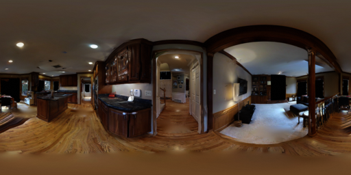
(a)

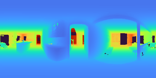
(b)

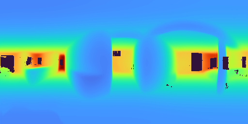
(c)

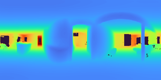
(d)

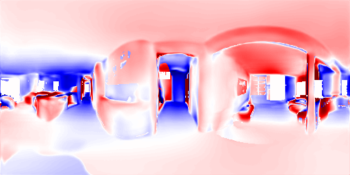
(e)

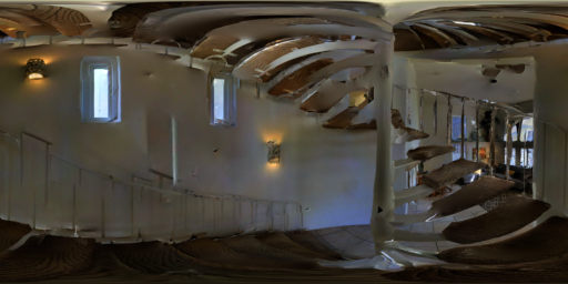
(f)

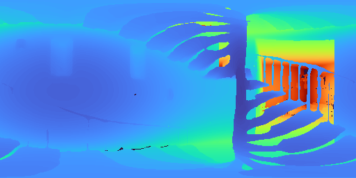
(g)

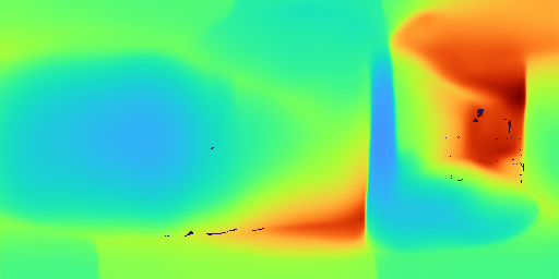
(h)

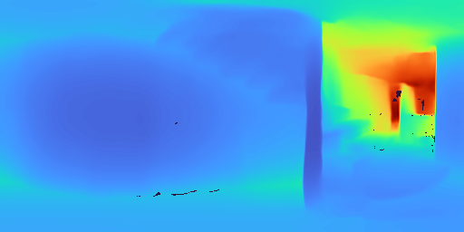
(i)

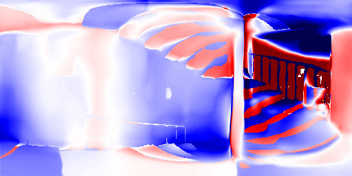
(j)

(k)

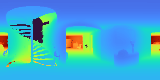
(l)

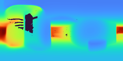
(m)

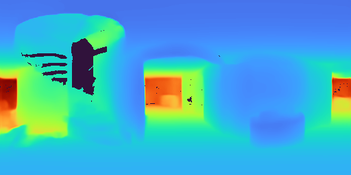
(n)

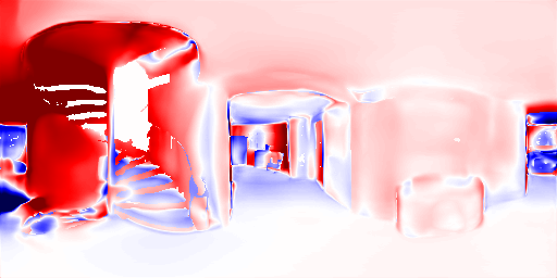
(o)

(p)

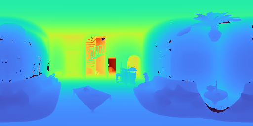
(q)

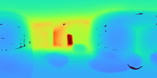
(r)

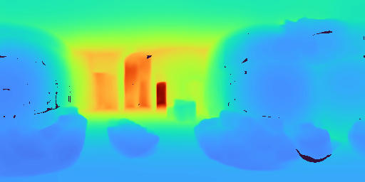
(s)

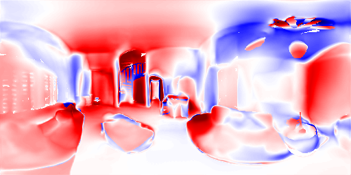
(t)

(a) Color

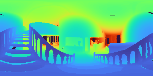
(b) Ground Truth Depth

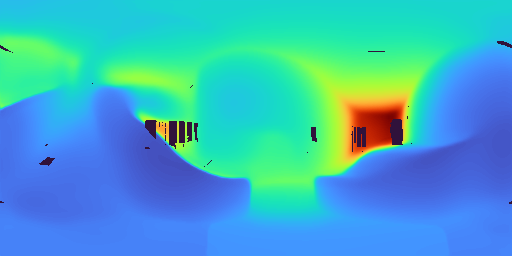
(c) ResNet Depth

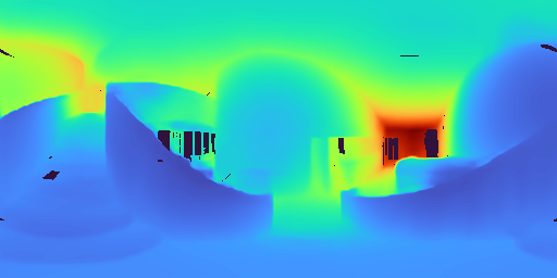
(d) ResNet_skip Depth

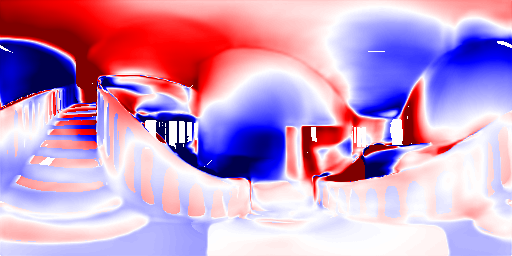
(e) Depth Advantage

Figure 4: Qualitative comparison between the ResNet and ResNet_skip architectures. On the right the advantage visualization shows with blue color the areas where the former performs better, and with red color the areas where the latter performs better. The color magnitude corresponds to the MAE difference between the two models, illustrating the performance deviation between the two models. The addition of skip connections allows ResNet_skip to capture finer-grained details.

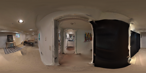
(a)

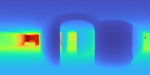
(b)

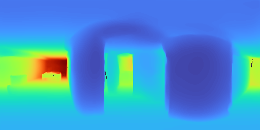
(c)

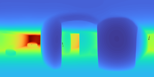
(d)

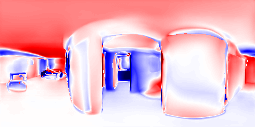
(e)

(f)

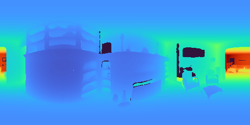
(g)

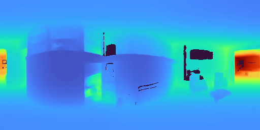
(h)

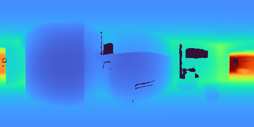
(i)

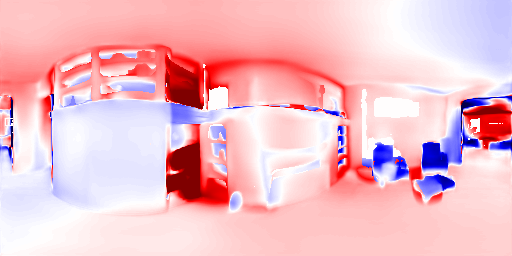
(j)

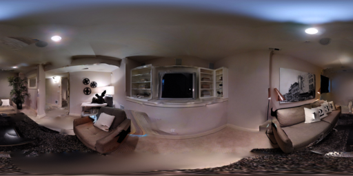
(k)

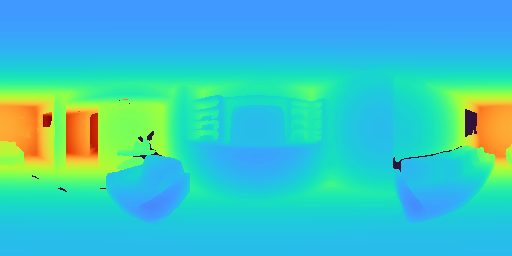
(l)

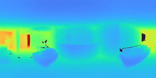
(m)

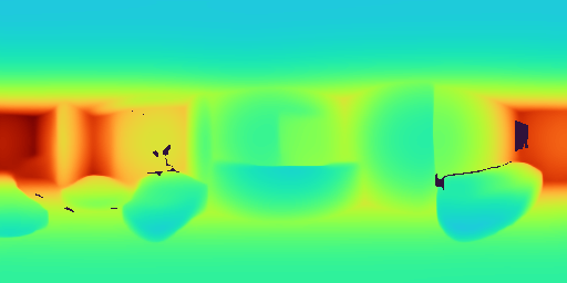
(n)

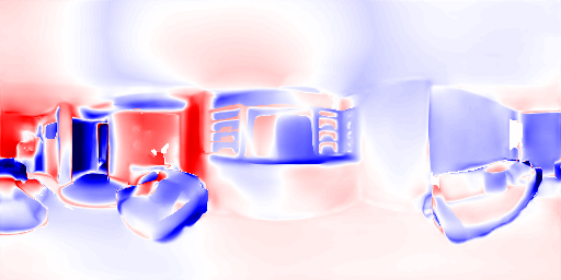
(o)

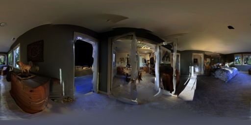
(p)

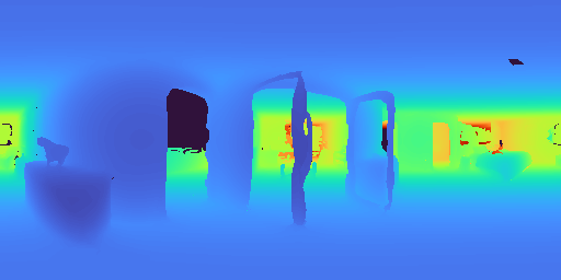
(q)

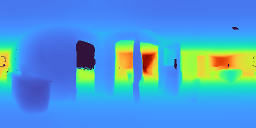
(r)

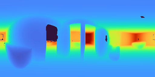
(s)

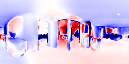
(t)

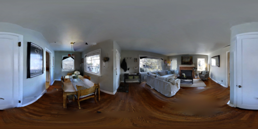
(a) Color

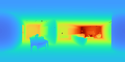
(b) Ground Truth Depth

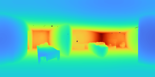
(c) Unet Depth

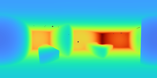
(d) Pnas Depth

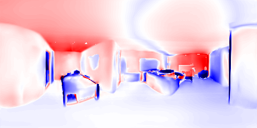
(e) Depth Advantage

Figure 5: Qualitative comparison between the UNet and Pnas architectures. On the right the advantage visualization shows with blue color the areas where the former performs better, and with red color the areas where the latter performs better. The color magnitude corresponds to the MAE difference between the two models, illustrating the performance deviation between the two models. Pnas provides smoother results while it is clear that UNet is able to capture finer-grained details.

(a)

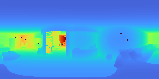
(b)

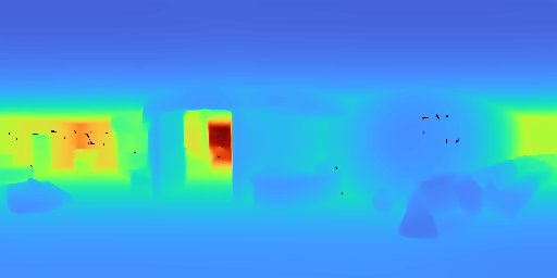
(c)

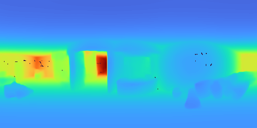
(d)

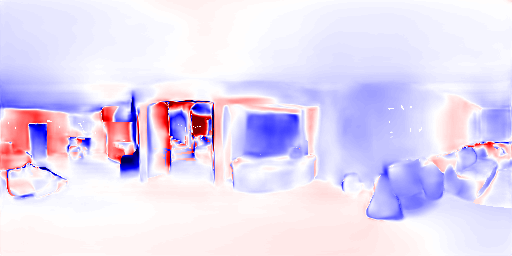
(e)

(f)

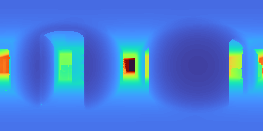
(g)

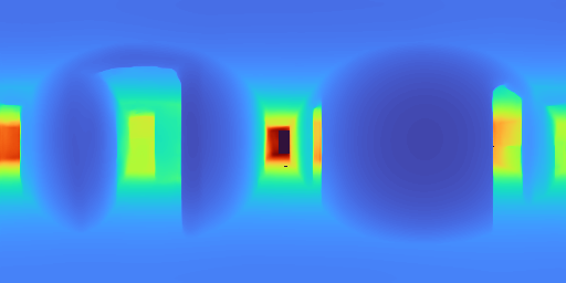
(h)

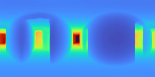
(i)

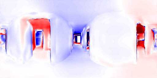
(j)

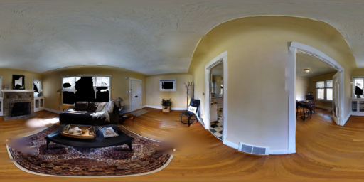
(k)

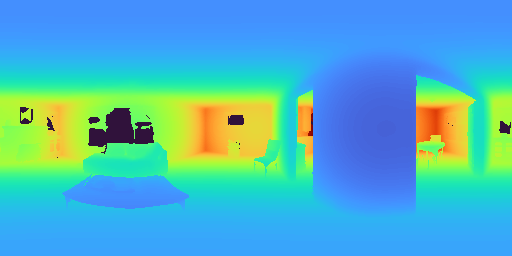
(l)

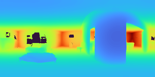
(m)

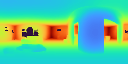
(n)

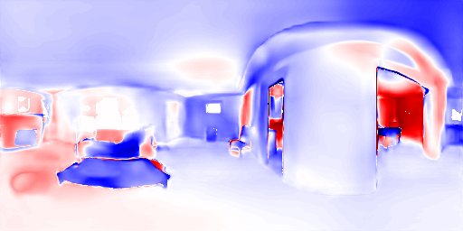
(o)

(p)

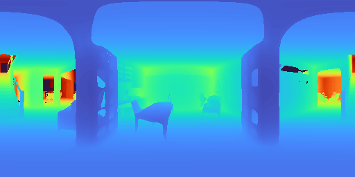
(q)

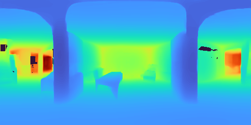
(r)

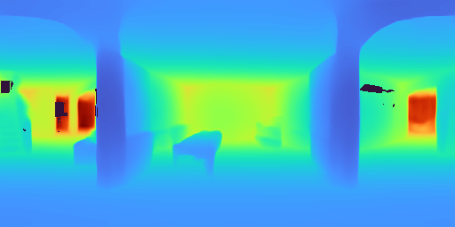
(s)

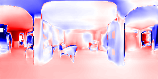
(t)

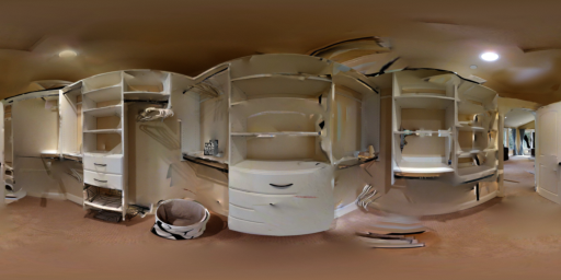
(a) Color

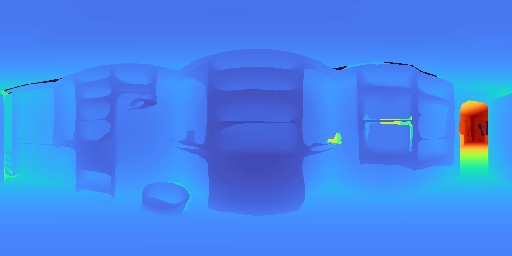
(b) Ground Truth Depth

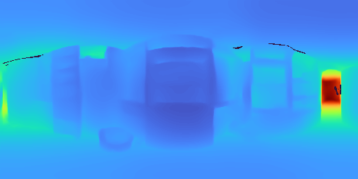
(c) Unet Depth

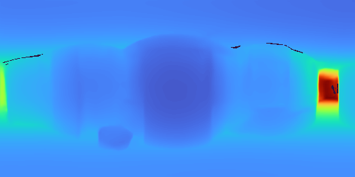
(d) ResNet_skip Depth

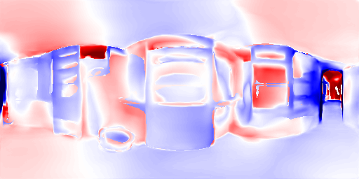
(e) Depth Advantage

Figure 6: Qualitative comparison between the UNet and ResNet_skip architectures. On the right the advantage visualization shows with blue color the areas where the former performs better, and with red color the areas where the latter performs better. The color magnitude corresponds to the MAE difference between the two models, illustrating the performance deviation between the two models.

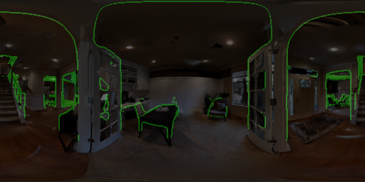
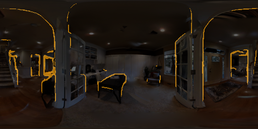
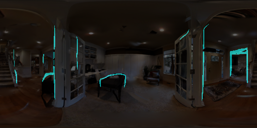
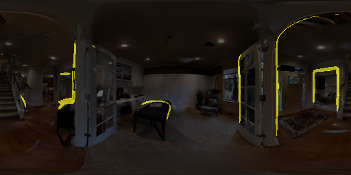
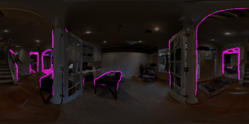
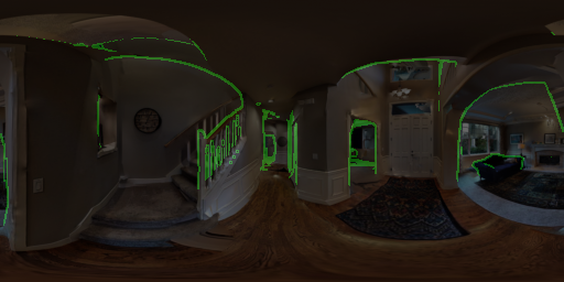
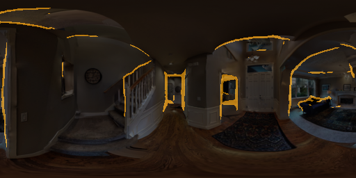
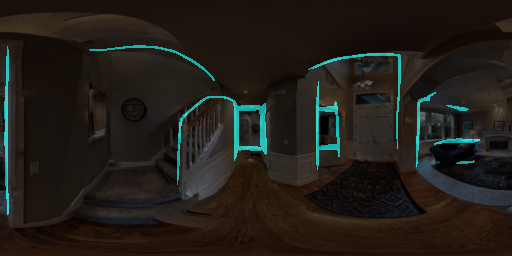
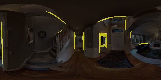
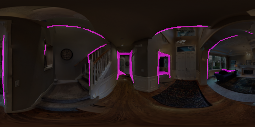
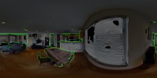
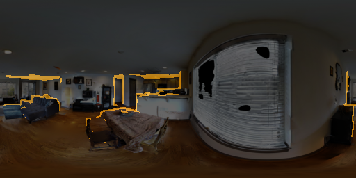
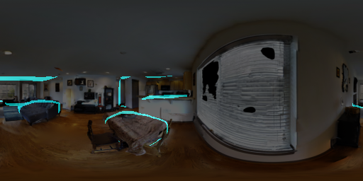
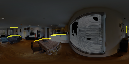
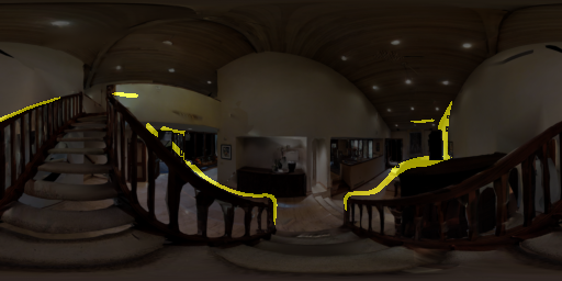
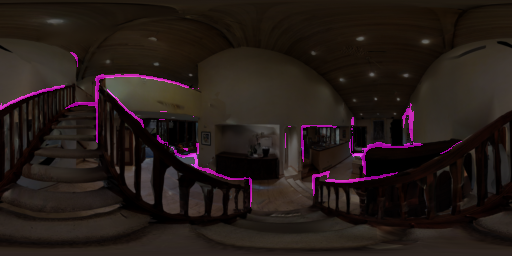
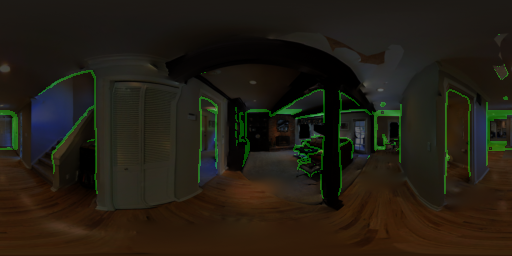
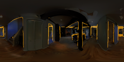
Figure 7: Boundary preservation qualitative comparison between the UNet, Pnas, ResNet and ResNet_skip models. Boundaries are extracted by applying a Canny edge detector [5] with predefined thresholds on normalized predicted depth maps, and then are blended with the original color panorama. From left to right: i) GT depth (green), ii) UNet (orange), iii) Pnas (cyan), iv) ResNet (yellow), and v) ResNet_skip (magenta).

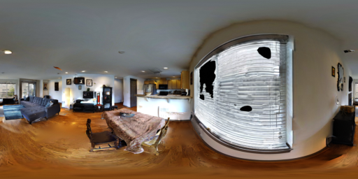
(a)

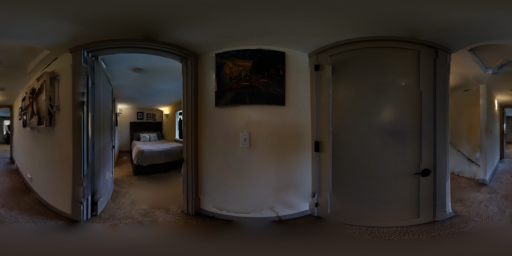
(b)

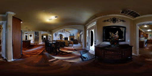
(c)

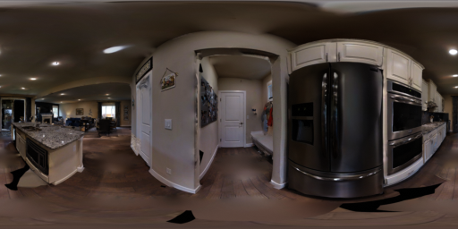
(d)

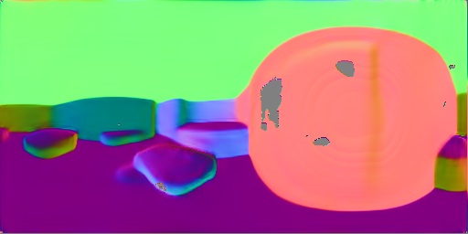
(e)

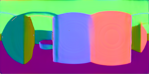
(f)

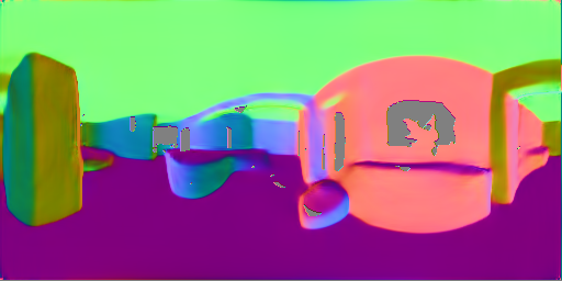
(g)

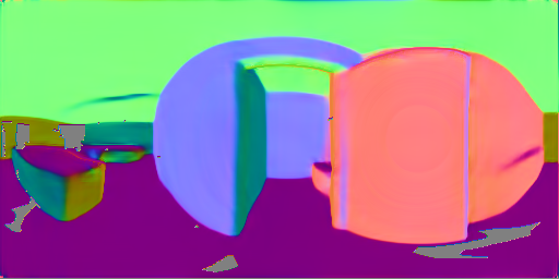
(h)

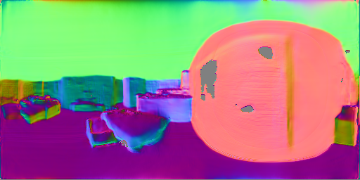
(i)

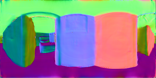
(j)

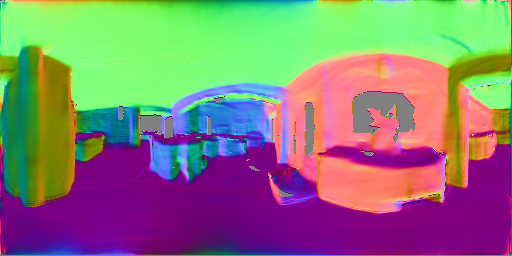
(k)

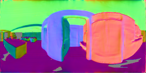
(l)

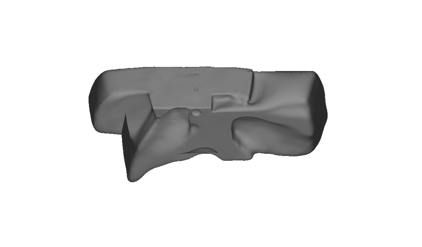
(m)

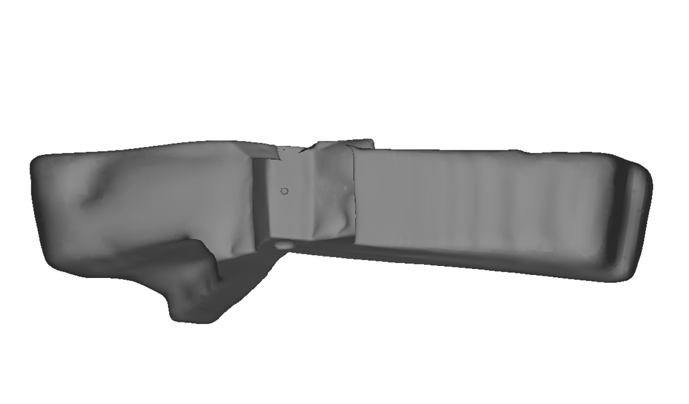
(n)

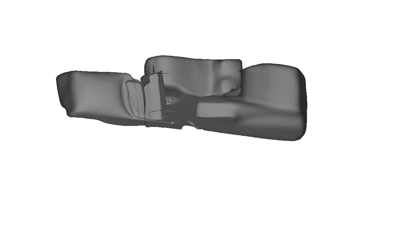
(o)

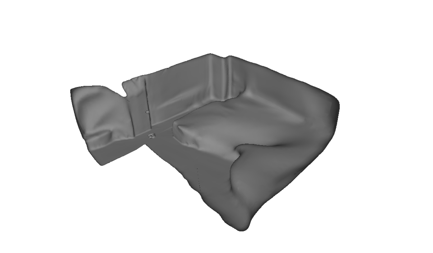
(p)

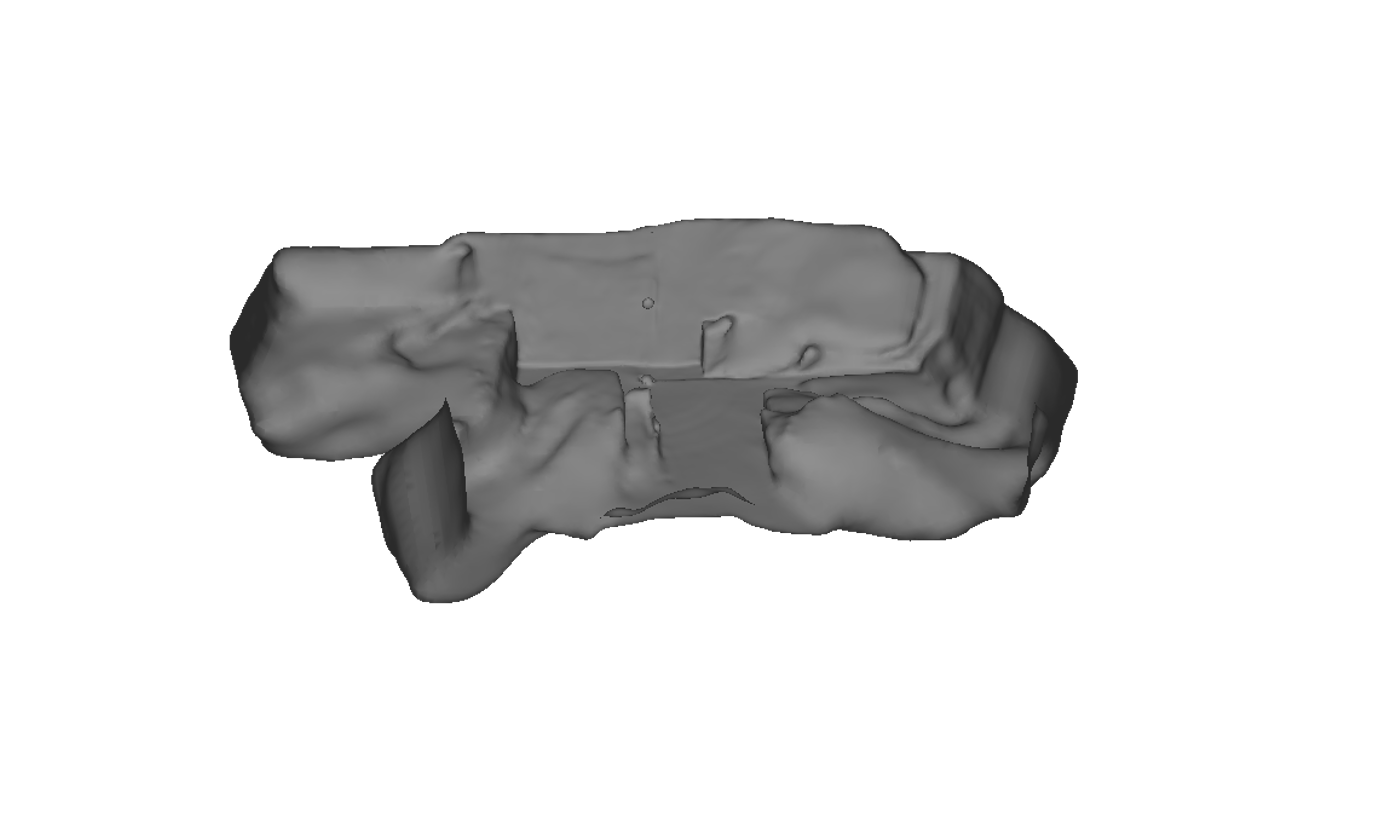
(q)

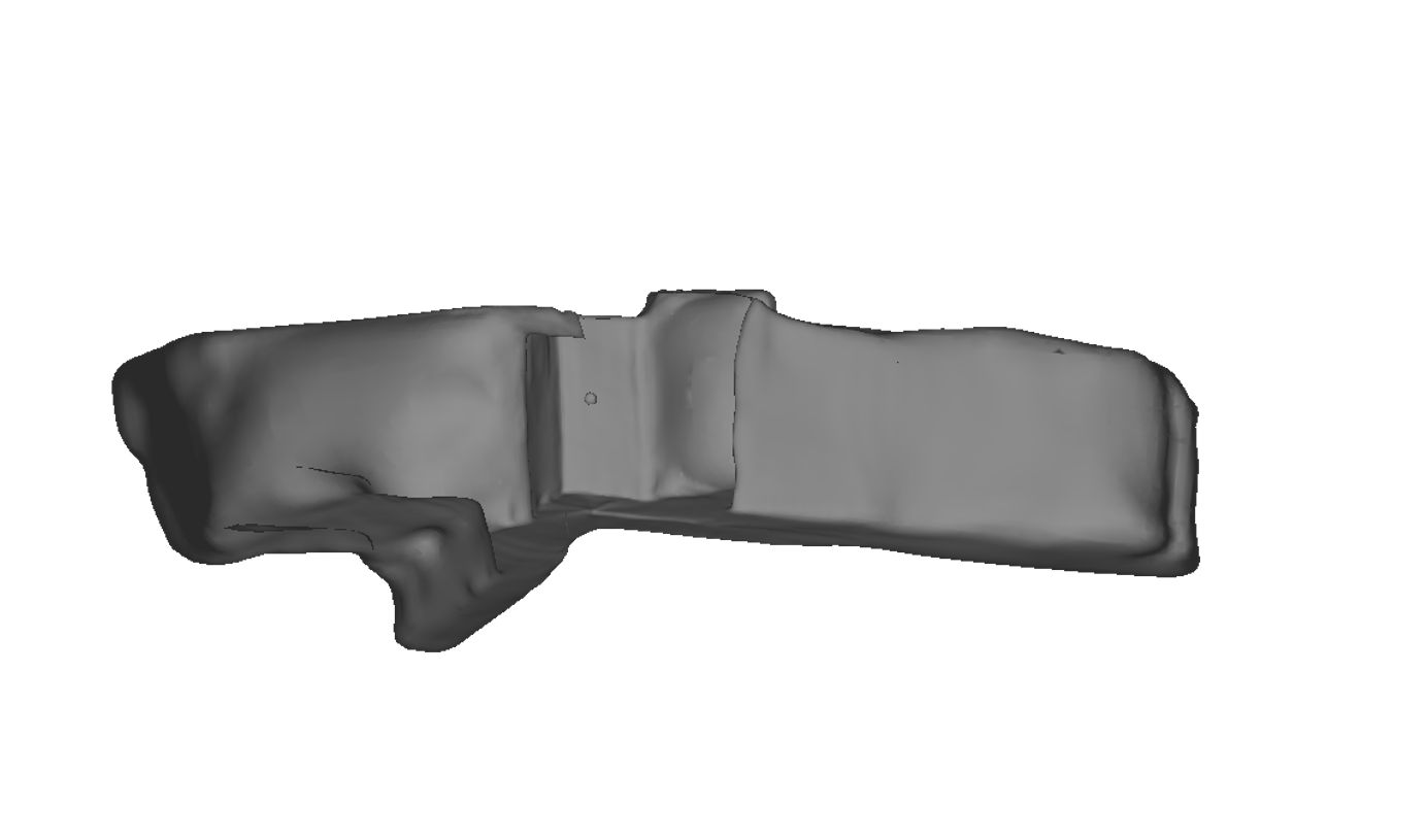
(r)

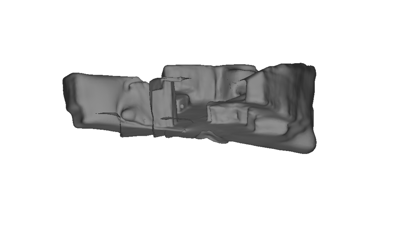
(s)

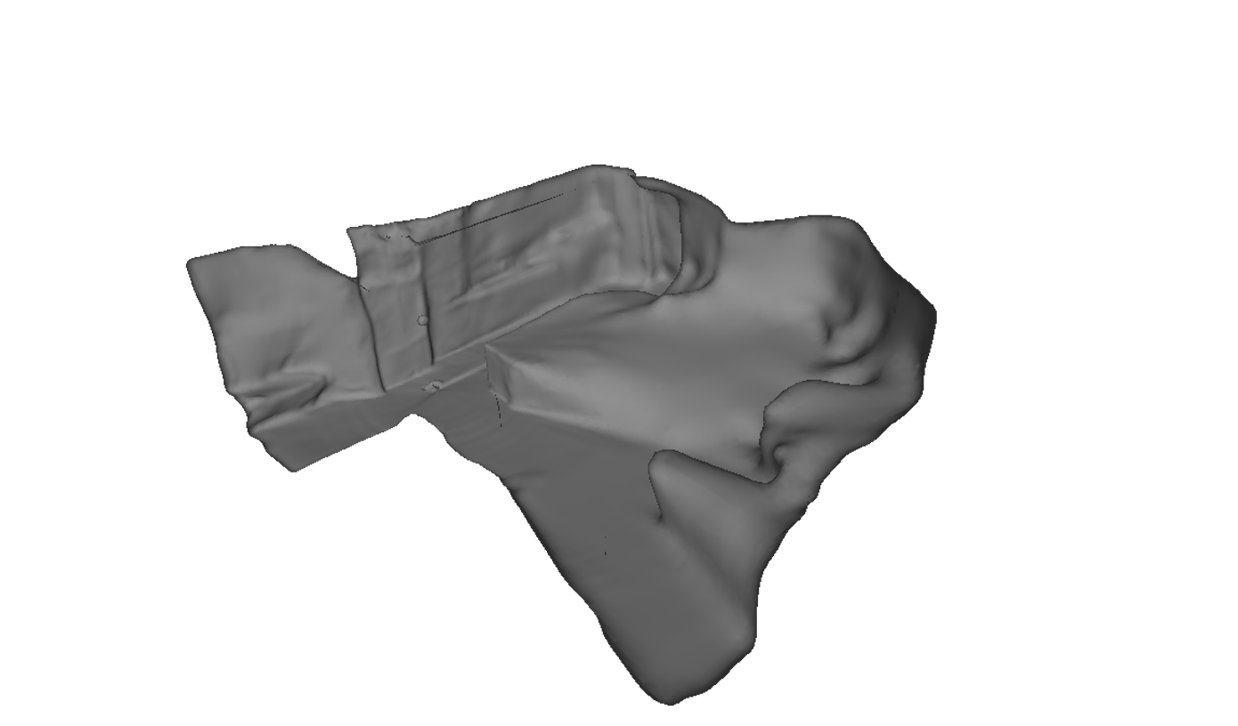
(t)

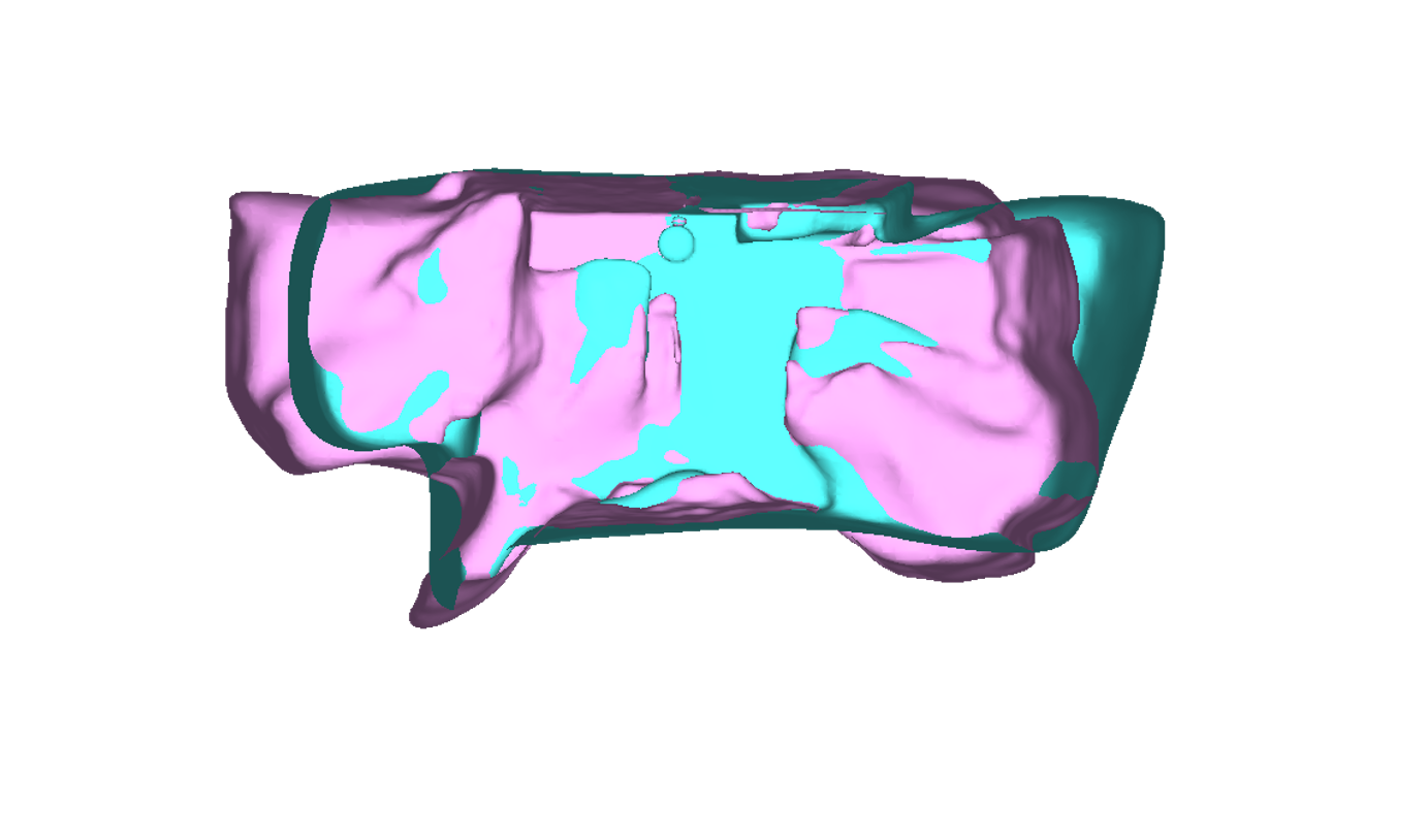
(u)

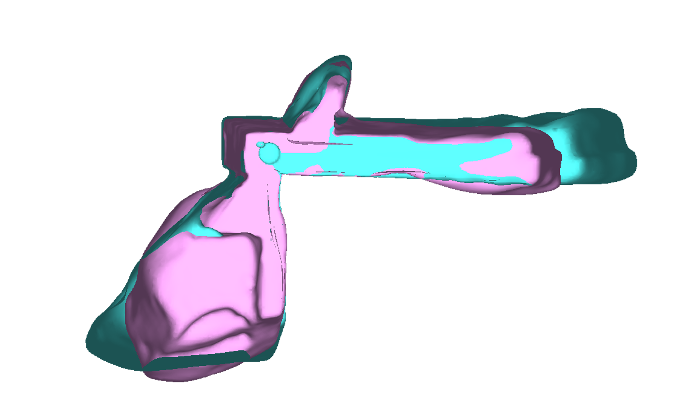
(v)

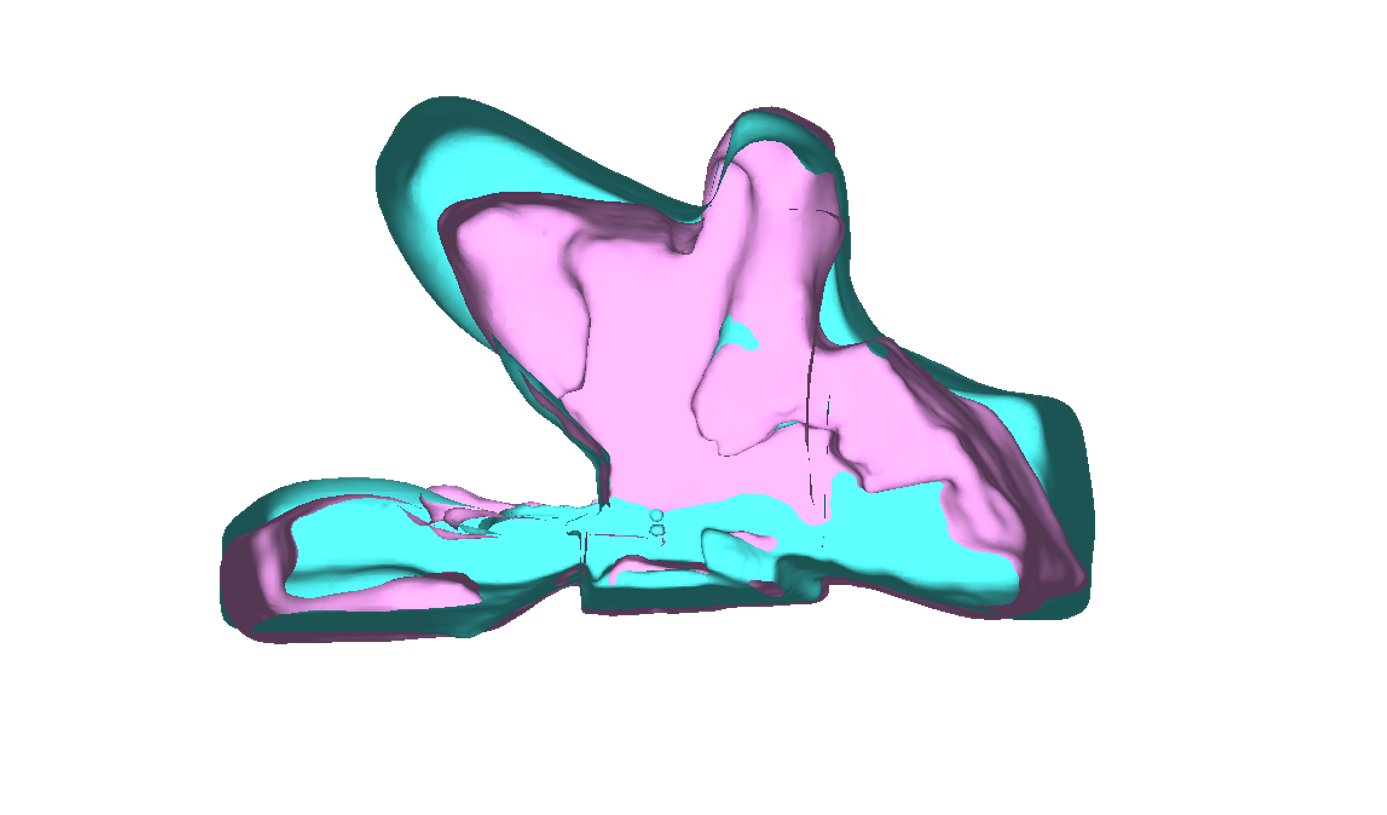
(w)

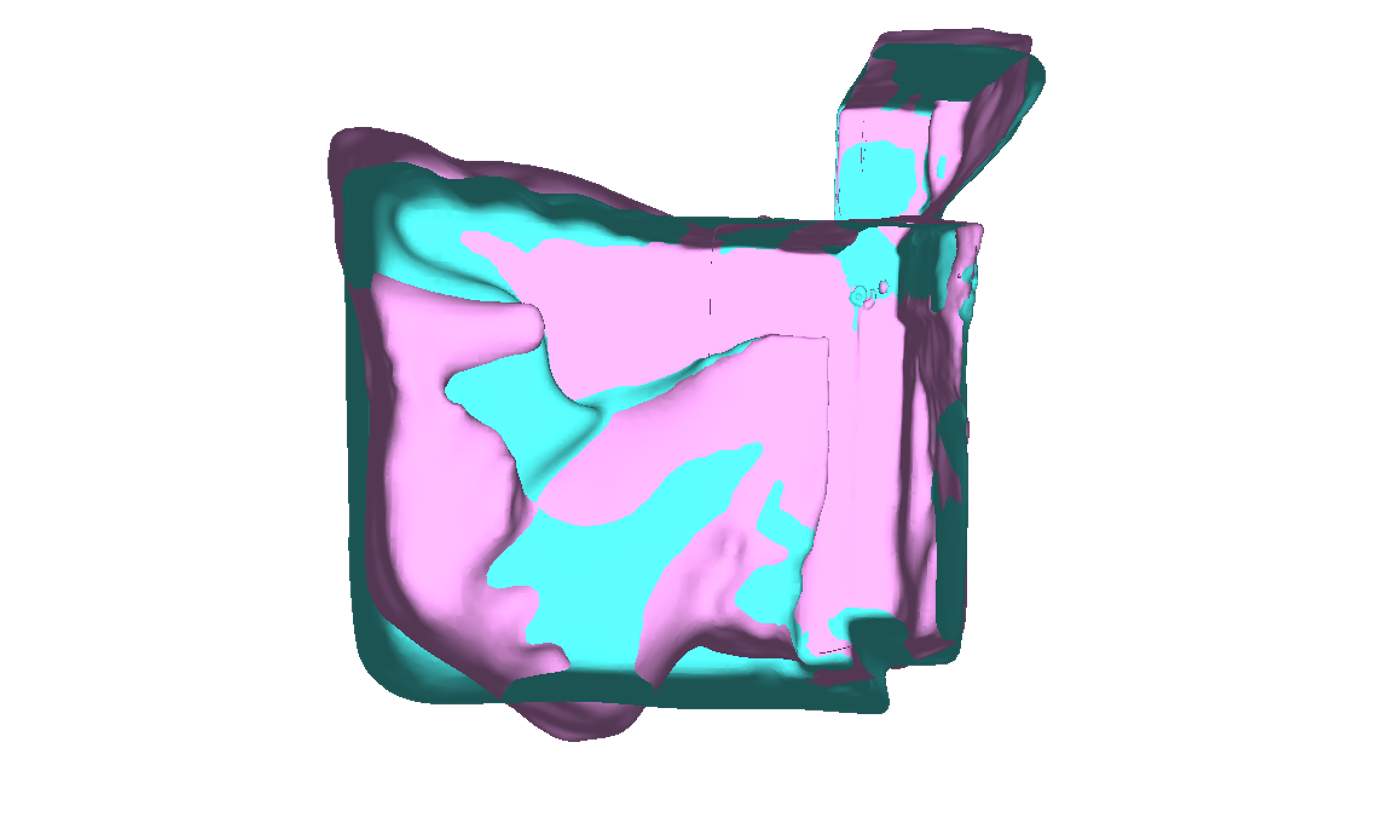
(x)

Figure 8: Qualitative comparison of the Pnas and UNet models in surface reconstruction. From top to bottom: i) input color panorama, ii) Pnas normal map from the estimated depth map, iii) UNet normal map, iv) Pnas Screened Poisson Surface Reconstruction [29] 3D surface reconstruction, v) UNet 3D surface reconstruction, vi) overlaid Pnas (cyan) and UNet (pink) 3D surface reconstructions from birds eye view.

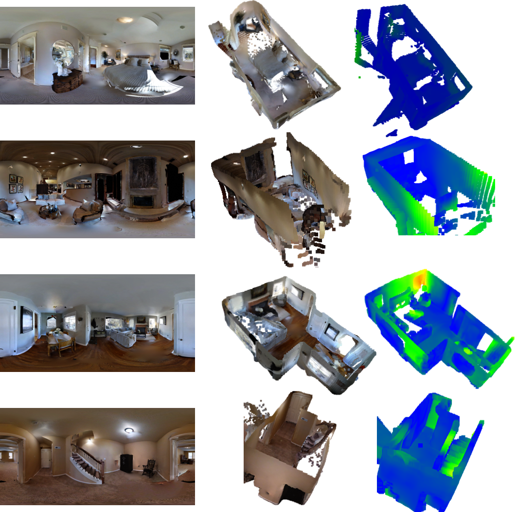
Figure 9: UNet qualitative results. From left to right: i) Input color panorama, ii) colored predicted point cloud, and iii) heatmap visualization of the c2c error on the ground truth point cloud.

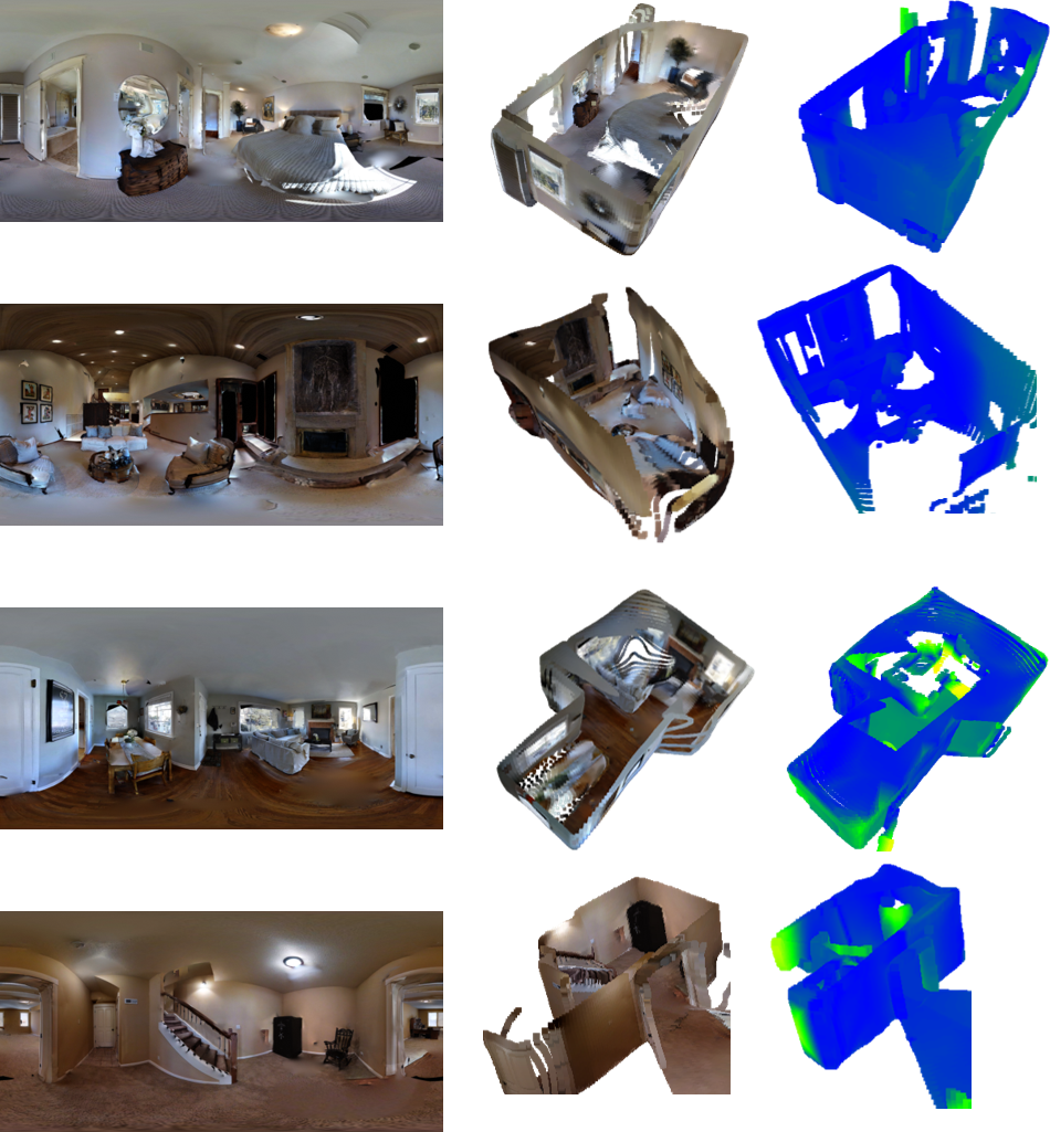
Figure 10: Pnas qualitative results. From left to right: i) Input color panorama, ii) colored predicted point cloud, and iii) heatmap visualization of the c2c error on the ground truth point cloud.

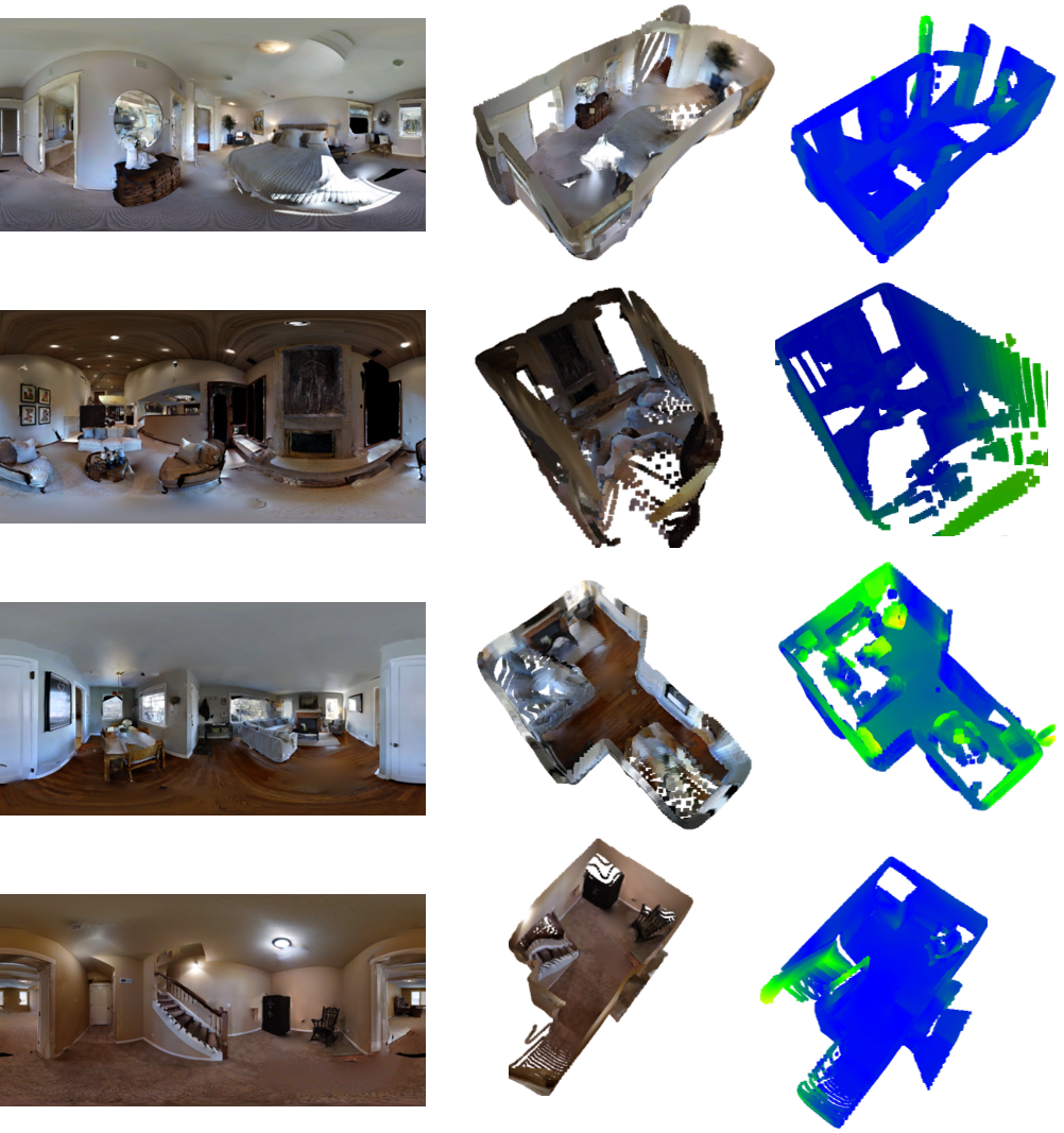
Figure 11: ResNet_skip qualitative results. From left to right: i) Input color panorama, ii) colored predicted point cloud, and iii) heatmap visualization of the c2c error on the ground truth point cloud.

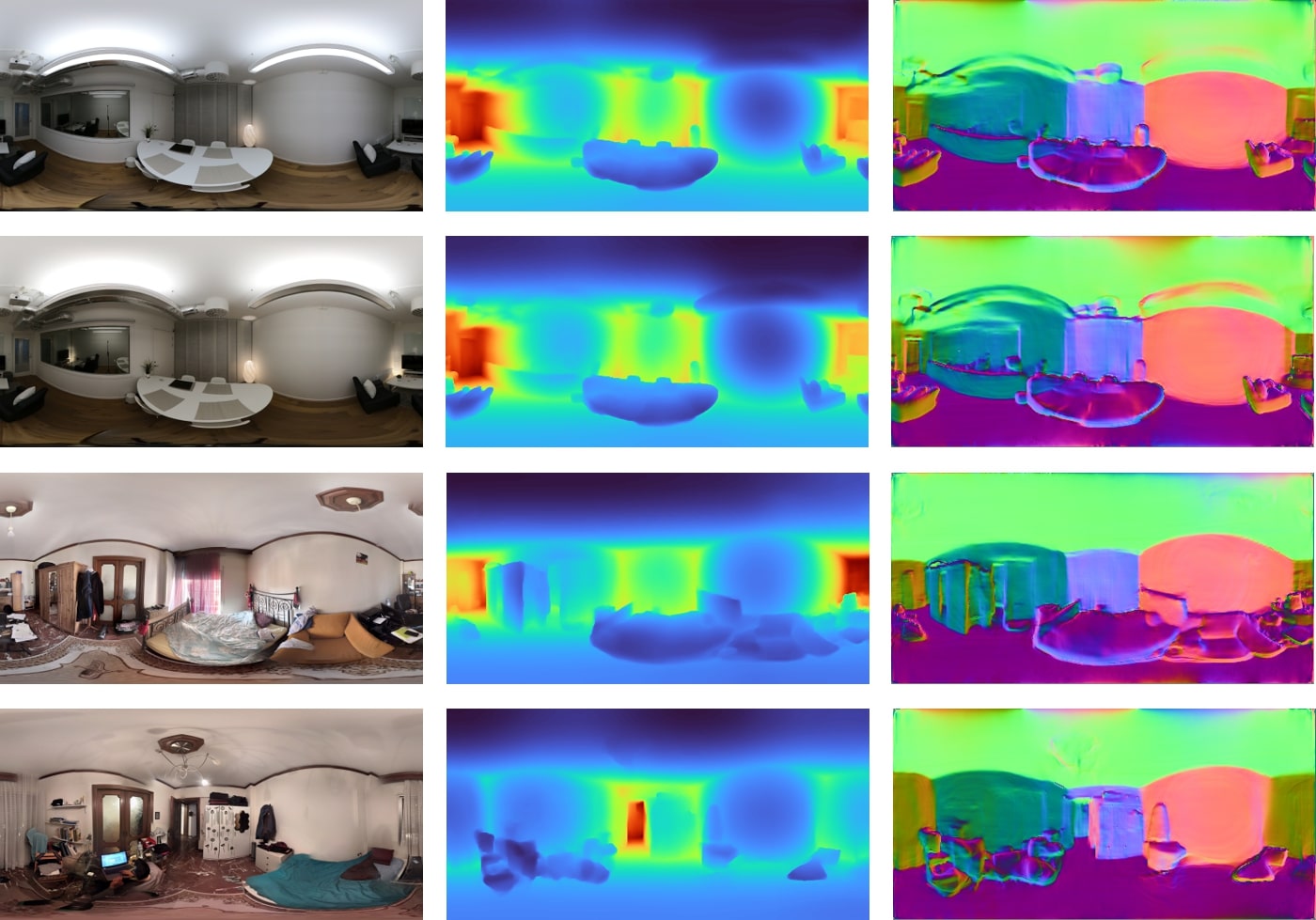
Figure 12: Qualitative results using the UNet model applied to in-the-wild real data captures. The top two rows are captures with a ${360}^{o}$ camera, while the bottom two rows are stitched panoramas from a mobile phone. From left to right: i) Input color panorama, ii) predicted depth, and iii) normals derived from the predicted depth.

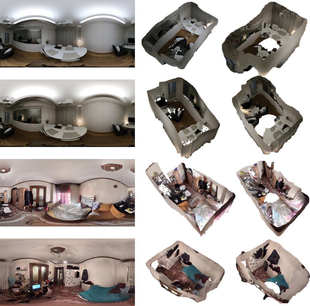
Figure 13: Qualitative results using in-the-wild data. On the left the input color panoramas are depicted. The two top rows are captured with a ${360}^{o}$ camera, while the bottom two rows are stitched panoramas from a mobile phone. The colored point clouds of the predicted depths from our UNet model (middle) and BiFuse [45] (right). Ceilings have been removed for visualization purposes.

References

- [1] Iro Armeni, Sasha Sax, Amir R Zamir, and Silvio Savarese. Joint 2d-3d-semantic data for indoor scene understanding. arXiv preprint arXiv:1702.01105, 2017.
- [2] Benjamin Attal, Selena Ling, Aaron Gokaslan, Christian Richardt, and James Tompkin. Matryodshka: Real-time 6dof video view synthesis using multi-sphere images. In European Conference on Computer Vision, pages 441–459. Springer, 2020.
- [3] Shariq Farooq Bhat, Ibraheem Alhashim, and Peter Wonka. Adabins: Depth estimation using adaptive bins. arXiv preprint arXiv:2011.14141, 2020.
- [4] Cesar Cadena, Yasir Latif, and Ian D Reid. Measuring the performance of single image depth estimation methods. In 2016 IEEE/RSJ International Conference on Intelligent Robots and Systems (IROS), pages 4150–4157. IEEE, 2016.
- [5] John Canny. A computational approach to edge detection. IEEE Transactions on pattern analysis and machine intelligence, (6):679–698, 1986.
- [6] Marcela Carvalho, Bertrand Le Saux, Pauline Trouvé-Peloux, Andrés Almansa, and Frédéric Champagnat. On regression losses for deep depth estimation. In 2018 25th IEEE International Conference on Image Processing (ICIP), pages 2915–2919. IEEE, 2018.
- [7] Angel Chang, Angela Dai, Thomas Funkhouser, Maciej Halber, Matthias Niebner, Manolis Savva, Shuran Song, Andy Zeng, and Yinda Zhang. Matterport3d: Learning from rgb-d data in indoor environments. In 7th IEEE International Conference on 3D Vision (3DV), pages 667–676. Institute of Electrical and Electronics Engineers Inc., 2018.
- [8] Weifeng Chen, Shengyi Qian, David Fan, Noriyuki Kojima, Max Hamilton, and Jia Deng. Oasis: A large-scale dataset for single image 3d in the wild. In Proceedings of the IEEE/CVF Conference on Computer Vision and Pattern Recognition, pages 679–688, 2020.
- [9] Xinjing Cheng, Peng Wang, Yanqi Zhou, Chenye Guan, and Ruigang Yang. Omnidirectional depth extension networks. In 2020 IEEE International Conference on Robotics and Automation (ICRA), pages 589–595. IEEE, 2020.
- [10] Paolo Cignoni, Claudio Rocchini, and Roberto Scopigno. Metro: measuring error on simplified surfaces. In Computer graphics forum, volume 17, pages 167–174. Wiley Online Library, 1998.
- [11] Piotr Dollár and C Lawrence Zitnick. Fast edge detection using structured forests. IEEE transactions on pattern analysis and machine intelligence, 37(8):1558–1570, 2014.
- [12] Marc Eder, Pierre Moulon, and Li Guan. Pano popups: Indoor 3d reconstruction with a plane-aware network. In 2019 International Conference on 3D Vision (3DV), pages 76–84. IEEE, 2019.
- [13] Marc Eder, True Price, Thanh Vu, Akash Bapat, and Jan-Michael Frahm. Mapped convolutions. arXiv preprint arXiv:1906.11096, 2019.
- [14] David Eigen, Christian Puhrsch, and Rob Fergus. Depth map prediction from a single image using a multi-scale deep network. In Advances in neural information processing systems, pages 2366–2374, 2014.
- [15] Brandon Yushan Feng, Wangjue Yao, Zheyuan Liu, and Amitabh Varshney. Deep depth estimation on 360° images with a double quaternion loss. In 2020 International Conference on 3D Vision (3DV), pages 524–533. IEEE, 2020.
- [16] Huan Fu, Mingming Gong, Chaohui Wang, Kayhan Batmanghelich, and Dacheng Tao. Deep ordinal regression network for monocular depth estimation. In Proceedings of the IEEE Conference on Computer Vision and Pattern Recognition, pages 2002–2011, 2018.
- [17] Daniel Girardeau-Montaut. Détection de changement sur des données géométriques tridimensionnelles. Theses, Télécom ParisTech, May 2006.
- [18] Clément Godard, Oisin Mac Aodha, and Gabriel J Brostow. Unsupervised monocular depth estimation with left-right consistency. In Proceedings of the IEEE Conference on Computer Vision and Pattern Recognition, pages 270–279, 2017.
- [19] Kaiming He, Xiangyu Zhang, Shaoqing Ren, and Jian Sun. Delving deep into rectifiers: Surpassing human-level performance on imagenet classification. In Proceedings of the IEEE international conference on computer vision, pages 1026–1034, 2015.
- [20] Kaiming He, Xiangyu Zhang, Shaoqing Ren, and Jian Sun. Identity mappings in deep residual networks. In European conference on computer vision, pages 630–645. Springer, 2016.
- [21] Junjie Hu, Mete Ozay, Yan Zhang, and Takayuki Okatani. Revisiting single image depth estimation: Toward higher resolution maps with accurate object boundaries. In 2019 IEEE Winter Conference on Applications of Computer Vision (WACV), pages 1043–1051. IEEE, 2019.
- [22] Gao Huang, Zhuang Liu, Laurens Van Der Maaten, and Kilian Q Weinberger. Densely connected convolutional networks. In Proceedings of the IEEE conference on computer vision and pattern recognition, pages 4700–4708, 2017.
- [23] Jinggang Huang, Ann B Lee, and David Mumford. Statistics of range images. In Proceedings IEEE Conference on Computer Vision and Pattern Recognition. CVPR 2000 (Cat. No. PR00662), volume 1, pages 324–331. IEEE, 2000.
- [24] Xun Huang and Serge Belongie. Arbitrary style transfer in real-time with adaptive instance normalization. In Proceedings of the IEEE International Conference on Computer Vision, pages 1501–1510, 2017.
- [25] Yu-Kai Huang, Tsung-Han Wu, Yueh-Cheng Liu, and Winston H Hsu. Indoor depth completion with boundary consistency and self-attention. In Proceedings of the IEEE/CVF International Conference on Computer Vision Workshops, pages 0–0, 2019.
- [26] Hualie Jiang, Zhe Sheng, Siyu Zhu, Zilong Dong, and Rui Huang. Unifuse: Unidirectional fusion for 360 panorama depth estimation. arXiv preprint arXiv:2102.03550, 2021.
- [27] Antonios Karakottas, Nikolaos Zioulis, Stamatis Samaras, Dimitrios Ataloglou, Vasileios Gkitsas, Dimitrios Zarpalas, and Petros Daras. 360° surface regression with a hyper-sphere loss. In 2019 International Conference on 3D Vision (3DV), pages 258–268. IEEE, 2019.
- [28] Kevin Karsch, Zicheng Liao, Jason Rock, Jonathan T Barron, and Derek Hoiem. Boundary cues for 3d object shape recovery. In Proceedings of the IEEE Conference on Computer Vision and Pattern Recognition, pages 2163–2170, 2013.
- [29] Michael Kazhdan and Hugues Hoppe. Screened poisson surface reconstruction. ACM Transactions on Graphics (ToG), 32(3):1–13, 2013.
- [30] Diederik P Kingma and Jimmy Ba. Adam: A method for stochastic optimization. arXiv preprint arXiv:1412.6980, 2014.
- [31] Tobias Koch, Lukas Liebel, Friedrich Fraundorfer, and Marco Korner. Evaluation of cnn-based single-image depth estimation methods. In Proceedings of the European Conference on Computer Vision (ECCV) Workshops, pages 0–0, 2018.
- [32] Iro Laina, Christian Rupprecht, Vasileios Belagiannis, Federico Tombari, and Nassir Navab. Deeper depth prediction with fully convolutional residual networks. In 2016 Fourth international conference on 3D vision (3DV), pages 239–248. IEEE, 2016.
- [33] Jae-Han Lee and Chang-Su Kim. Multi-loss rebalancing algorithm for monocular depth estimation. In Proceedings of the 2020 European Conference on Computer Vision (ECCV), Glasgow, UK, pages 23–28, 2020.
- [34] Jin Lei, Xu Yanyu, Zheng Jia, Zhang Junfei, Tang Rui, Xu Shugong, Yu Jingyi, and Gao Shenghua. Geometric structure based and regularized depth estimation from indoor imagery. In Proceedings of the IEEE Conference on Computer Vision and Pattern Recognition (CVPR), 2020.
- [35] Zhengqi Li and Noah Snavely. Megadepth: Learning single-view depth prediction from internet photos. In Proceedings of the IEEE Conference on Computer Vision and Pattern Recognition, pages 2041–2050, 2018.
- [36] Chenxi Liu, Barret Zoph, Maxim Neumann, Jonathon Shlens, Wei Hua, Li-Jia Li, Li Fei-Fei, Alan Yuille, Jonathan Huang, and Kevin Murphy. Progressive neural architecture search. In Proceedings of the European conference on computer vision (ECCV), pages 19–34, 2018.
- [37] moai: Accelerating modern data-driven workflows. https://github.com/ai-in-motion/moai, 2021.
- [38] Alejandro Newell, Kaiyu Yang, and Jia Deng. Stacked hourglass networks for human pose estimation. In European conference on computer vision, pages 483–499. Springer, 2016.
- [39] Michaël Ramamonjisoa, Yuming Du, and Vincent Lepetit. Predicting sharp and accurate occlusion boundaries in monocular depth estimation using displacement fields. In Proceedings of the IEEE/CVF Conference on Computer Vision and Pattern Recognition, pages 14648–14657, 2020.
- [40] Rene Ranftl, Katrin Lasinger, David Hafner, Konrad Schindler, and Vladlen Koltun. Towards robust monocular depth estimation: Mixing datasets for zero-shot cross-dataset transfer. IEEE Transactions on Pattern Analysis and Machine Intelligence, 2020.
- [41] Olaf Ronneberger, Philipp Fischer, and Thomas Brox. U-net: Convolutional networks for biomedical image segmentation. In International Conference on Medical image computing and computer-assisted intervention, pages 234–241. Springer, 2015.
- [42] Cheng Sun, Chi-Wei Hsiao, Min Sun, and Hwann-Tzong Chen. Horizonnet: Learning room layout with 1d representation and pano stretch data augmentation. In Proceedings of the IEEE Conference on Computer Vision and Pattern Recognition, pages 1047–1056, 2019.
- [43] Cheng Sun, Min Sun, and Hwann-Tzong Chen. Hohonet: 360 indoor holistic understanding with latent horizontal features. arXiv preprint arXiv:2011.11498, 2020.
- [44] Keisuke Tateno, Nassir Navab, and Federico Tombari. Distortion-aware convolutional filters for dense prediction in panoramic images. In Proceedings of the European Conference on Computer Vision (ECCV), pages 707–722, 2018.
- [45] Fu-En Wang, Yu-Hsuan Yeh, Min Sun, Wei-Chen Chiu, and Yi-Hsuan Tsai. Bifuse: Monocular 360 depth estimation via bi-projection fusion. In Proceedings of the IEEE/CVF Conference on Computer Vision and Pattern Recognition, pages 462–471, 2020.
- [46] Rui Wang, David Geraghty, Kevin Matzen, Richard Szeliski, and Jan-Michael Frahm. Vplnet: Deep single view normal estimation with vanishing points and lines. In Proceedings of the IEEE/CVF Conference on Computer Vision and Pattern Recognition, pages 689–698, 2020.
- [47] Huikai Wu, Shuai Zheng, Junge Zhang, and Kaiqi Huang. Fast end-to-end trainable guided filter. In Proceedings of the IEEE Conference on Computer Vision and Pattern Recognition, pages 1838–1847, 2018.
- [48] Fei Xia, Amir R Zamir, Zhiyang He, Alexander Sax, Jitendra Malik, and Silvio Savarese. Gibson env: Real-world perception for embodied agents. In Proceedings of the IEEE Conference on Computer Vision and Pattern Recognition, pages 9068–9079, 2018.
- [49] Ke Xian, Jianming Zhang, Oliver Wang, Long Mai, Zhe Lin, and Zhiguo Cao. Structure-guided ranking loss for single image depth prediction. In Proceedings of the IEEE/CVF Conference on Computer Vision and Pattern Recognition, pages 611–620, 2020.
- [50] Mai Xu, Chen Li, Shanyi Zhang, and Patrick Le Callet. State-of-the-art in 360 video/image processing: Perception, assessment and compression. IEEE Journal of Selected Topics in Signal Processing, 14(1):5–26, 2020.
- [51] Wei Yin, Yifan Liu, Chunhua Shen, and Youliang Yan. Enforcing geometric constraints of virtual normal for depth prediction. In Proceedings of the IEEE/CVF International Conference on Computer Vision, pages 5684–5693, 2019.
- [52] Wei Zeng, Sezer Karaoglu, and Theo Gevers. Joint 3d layout and depth prediction from a single indoor panorama image. In European Conference on Computer Vision, pages 666–682. Springer, 2020.
- [53] Jia Zheng, Junfei Zhang, Jing Li, Rui Tang, Shenghua Gao, and Zihan Zhou. Structured3d: A large photo-realistic dataset for structured 3d modeling. In Proceedings of The European Conference on Computer Vision (ECCV), 2020.
- [54] Nikolaos Zioulis, Federico Alvarez, Dimitrios Zarpalas, and Petros Daras. Single-shot cuboids: Geodesics-based end-to-end manhattan aligned layout estimation from spherical panoramas. arXiv preprint arXiv:2102.03939, 2021.
- [55] Nikolaos Zioulis, Antonis Karakottas, Dimitrios Zarpalas, Federico Alvarez, and Petros Daras. Spherical view synthesis for self-supervised 360° depth estimation. In 2019 International Conference on 3D Vision (3DV), pages 690–699. IEEE, 2019.
- [56] Nikolaos Zioulis, Antonis Karakottas, Dimitrios Zarpalas, and Petros Daras. Omnidepth: Dense depth estimation for indoors spherical panoramas. In Proceedings of the European Conference on Computer Vision (ECCV), pages 448–465, 2018.