Zero-Shot Out-of-Distribution Detection Based on the Pre-trained Model CLIP

Abstract

In an out-of-distribution (OOD) detection problem, samples of known classes (also called in-distribution classes) are used to train a special classifier. In testing, the classifier can (1) classify the test samples of known classes to their respective classes and also (2) detect samples that do not belong to any of the known classes (i.e., they belong to some unknown or OOD classes). This paper studies the problem of zero-shot out-of-distribution (OOD) detection, which still performs the same two tasks in testing but has no training except using the given known class names. This paper proposes a novel and yet simple method (called ZOC) to solve the problem. ZOC builds on top of the recent advances in zero-shot classification through multi-modal representation learning. It first extends the pre-trained language-vision model CLIP by training a text-based image description generator on top of CLIP. In testing, it uses the extended model to generate candidate unknown class names for each test sample and computes a confidence score based on both the known class names and candidate unknown class names for zero-shot OOD detection. Experimental results on 5 benchmark datasets for OOD detection demonstrate that ZOC outperforms the baselines by a large margin.

Introduction

The primary assumption in conventional supervised learning is that the samples encountered at the test time are from the same classes (called known or seen classes) that the model has observed and learned during training. However, this assumption, called the closed-world assumption (Fei and Liu 2016), is often violated when a machine learning model is deployed in the real world; i.e., in addition to the seen classes, samples from unseen classes may appear at test. The seen class samples are referred to as the in-distribution samples while unseen class samples are called out-of-distribution (OOD) samples. It is crucial for an intelligent ML model to detect OOD samples specially in safety-critical applications such as autonomous driving or healthcare since detecting OOD samples as in-distribution ones in such applications can have catastrophic consequences.

There are different directions in the literature tackling the OOD detection problem. The earlier methods are mainly based on SVMs (Scheirer et al. 2012; Scheirer, Jain, and Boult 2014; Fei and Liu 2016). Recent methods are mainly based on deep learning (Shu, Xu, and Liu 2017, 2018; Xu et al. 2019; Shu et al. 2021; Liang, Li, and Srikant 2017; Perera et al. 2020; Miller et al. 2021) and try to solve the problem from different perspectives. Some discriminative models perform the detection by calibrating the confidence of the closed-world classifier built using seen or in-distribution classes (Bendale and Boult 2016). Liang, Li, and Srikant (2017) proposed to use temperature scaling on the softmax score and perform post-processing on the test data to detect the OOD data. Lee et al. (2017) proposed a special training method for building closed-world classifiers that can also detect OOD samples at inference (Lee et al. 2017). Some generative models synthesize samples to represent possible unseen classes (Neal et al. 2018). These samples are then used to learn a $K+1$ classifier where the space of unseen is assumed to be enclosed in the extra class. Other generative methods also exist (Andrews, Morton, and Griffin 2016; Chen et al. 2017), which detect OOD samples based on the reconstruction error of the trained generative model for unseen samples. Perera et al. (2020) is a recent hybrid model based on generative-discriminative features.

Regardless of the approaches, the results on OOD detection benchmarks indicate that the OOD detection performance is directly affected by the accuracy of the closed-world classifier. Particularly, when the closed-world classifier does not use pre-trained models, it is essential to train an accurate classifier from scratch for a descent OOD detection performance. None of the aforementioned techniques use pre-trained models as the backbone of their closed-world classifiers. In fact, most of them essentially try to bound the hidden space representing the in-distribution classes. Then, the outer space can be considered as the OOD space.

This paper defines the zero-shot OOD detection problem to take advantage of pre-trained models. Given a set of seen class labels/names, $\mathcal{Y}_{s}$, the goal of zero-shot OOD detection is to 1) classify each seen class test sample to one of the seen classes and 2) detect samples that do not belong to any of the seen classes. These are done based on only the names of the seen classes in $\mathcal{Y}_{s}$. There is no given training data of the seen classes and thus no closed-world classifier is built.

CLIP (Radford et al. 2021) is a recently proposed pre-trained language-vision model from OpenAI for zero-shot (closed-world) image classification. It is trained by directly using the raw text for learning visual representations. CLIP is a multi-modal (image and text) transformer model which is trained by contrastive learning on a large set of 400 million image and caption pairs collected from the Internet. The rich feature space shared by both image and text data enables zero-shot transfer to a range of down-stream tasks including image classification. CLIP model has an image encoder and a text encoder. Its zero-shot classification is done by matching the features from the image encoder to a set of text features from the text encoder. The text with the highest similarity score to the image is its predicted label.

Although using CLIP eliminates the need for training a closed-world classifier, it does not possess the OOD detection functionality in its original form. That is, it will match any given image to one of the given seen class labels. Therefore, to function in an OOD setting, we need to present another set of candidate labels in addition to the seen class labels/names. The proposed method, called ZOC (Zero-shot OOD detection based on CLIP), does not need this set of candidate labels to represent possible OOD labels as ZOC can dynamically generate candidate OOD labels for inference. ZOC works based on comparing the similarity of the semantic meaning of the given image to seen labels vs its similarity to some generated candidate labels. For this to work, we need a text generator to generate candidate labels, which does not exist in CLIP. To the best of our knowledge, existing OOD detection baselines either 1) need to train a closed-world classifier on seen classes using their labeled training data or 2) have prior knowledge about unseen classes for detection. ZOC requires neither of the two and therefore it is the first work performing zero-shot OOD detection. In this work, we propose to:

• Extend the CLIP model by training a textual description generator on top of CLIP’s image encoder.

• Use the output of this generator as unseen candidate labels for a given test image.

• Define an OOD confidence score based on the similarity of the input test image to the union of the $seen$ labels and the $generated$ labels.

Our experimental results show that this simple method outperforms many state-of-the-art fully supervised OOD detection baselines trained using benchmark datasets. In addition to the supervised baselines, ZOC also outperforms the baselines that use the same pre-trained backbone model as ZOC.

Related Work

General Out-of-Distribution Detection

The terms Out-Of-Distribution (OOD) detection, Open Set Detection and Open World Classification are interchangeably used in the literature. In most papers about open set detection or open world classification, seen and unseen classes in evaluation are often two splits of the same dataset (Fei and Liu 2016; Shu, Xu, and Liu 2017; Bendale and Boult 2016; Oza and Patel 2019; Perera et al. 2020; Miller et al. 2021; Pernici et al. 2018; Xu et al. 2019). For OOD detection, all seen classes (e.g., images of hand-written digits) are regarded as a single or multiple in-distribution classes, while the OOD data to be detected are from a different dataset (e.g., images of animals) (Hendrycks and Gimpel 2016; Liang, Li, and Srikant 2017; Lee et al. 2018). That is, the OOD classes are often visually completely dissimilar to in-distribution classes. However, there is no fundamental difference between OOD detection and open set detection or open world classification. This paper refers all of them as OOD detection.

We note that some OOD detection techniques are based on the idea of outlier exposure. These methods either assume the direct access to a small subset of the actual test OOD data at training (Liang, Li, and Srikant 2017) or rely on a large set of data points used as outliers at training (Hendrycks, Mazeika, and Dietterich 2018). However, most OOD detection methods, including ours, do not see any samples from unseen OOD classes before deployment. Recently, some authors made a distinction between hard and easy OOD detection problems (Winkens et al. 2020). That is, detecting OOD CIFAR100 from in-distribution CIFAR10 is considered as a near-OOD (hard) problem as the two datasets contain visually similar categories. Likewise, detecting OOD CIFAR10 from in-distribution SVHN (photographed digits) is considered as a far-OOD (easy) problem because their categories are visually and semantically very different. Despite this distinction, using a validation set from the OOD data to tune the model parameters, is a common practice in many OOD detection approaches. In this paper, we solve the near-OOD (or hard) problem in the zero-shot setting without using any validation OOD data.

Transformer Model for OOD Detection

The success of pre-trained transformer models (Vaswani et al. 2017; Devlin et al. 2018) in the natural language domain has motivated researchers to analyze their performance for out-of-distribution or out-of-scope detection in real world applications. Hendrycks et al. (2020) studies the OOD generalization and OOD detection performance of BERT for a range of NLP tasks. Their evaluation acknowledges that a pre-trained transformer improves OOD detection upon conventional models which are merely as good as a random detector for OOD detection.

The vision transformer model (ViT) (Dosovitskiy et al. 2020) works in a similar way to a language transformer, i.e., it divides an image to consecutive patches and then uses a regular transformer encoder to process these flattened patches as a sequence. ViT achieves on par or better performance than CNN-based methods like ResNets. A recent study (Fort, Ren, and Lakshminarayanan 2021) analyzed the reliability of OOD detection in ViT models. The authors show that ViT pre-trained models fine-tuned on an in-distribution dataset significantly improve near OOD detection tasks. In addition, this work is the most related work to ours in the sense that it performs zero-shot OOD detection through CLIP. However, Fort, Ren, and Lakshminarayanan (2021) assumed that a set of unseen labels are given as some weak information about OOD data which is not practical in real world scenarios.

Method

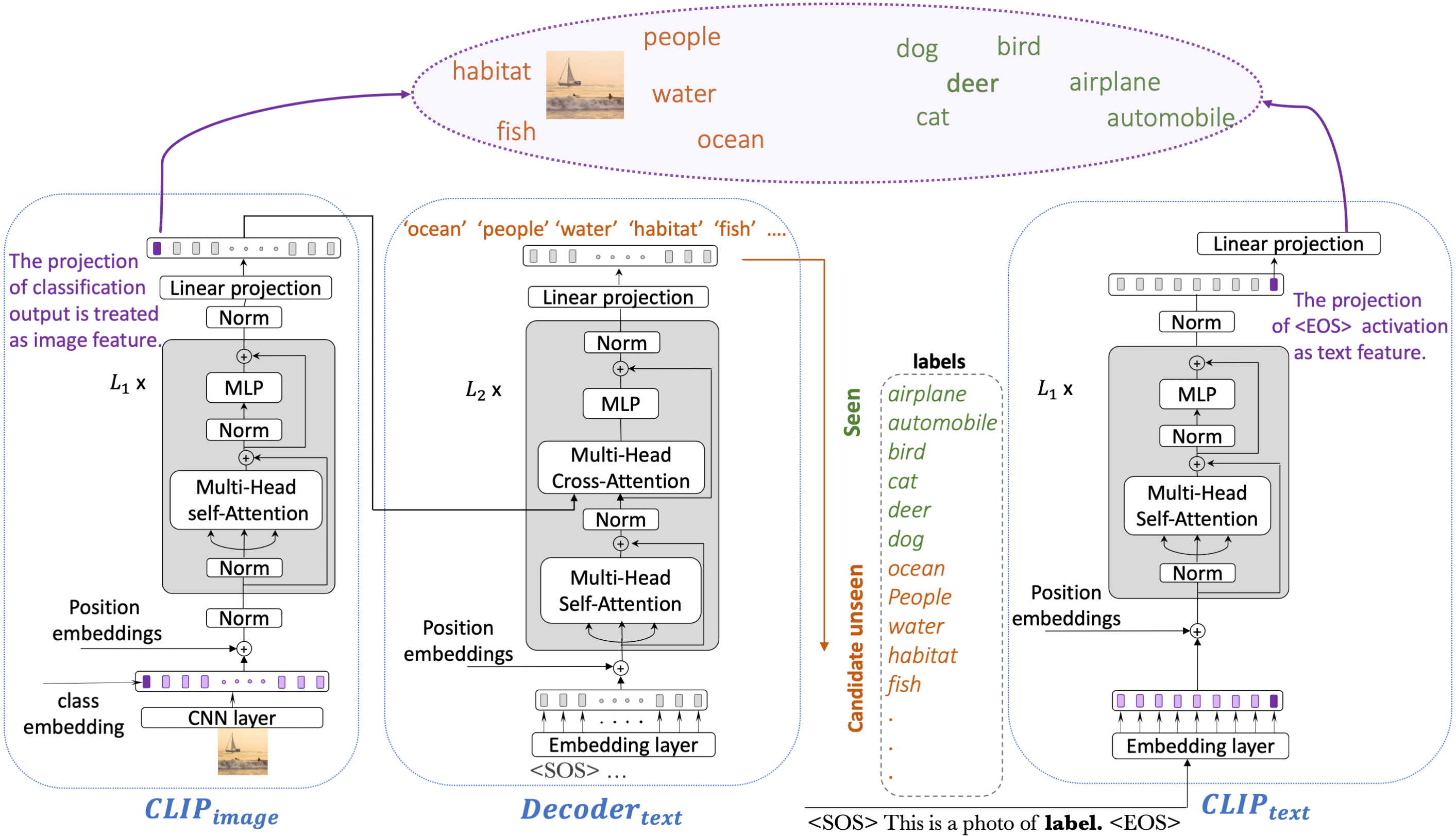
Figure 1: The diagram illustrates the inference steps of ZOC for a sample from an unseen class ‘boat’. The available seen class labels (shown in green) are $\mathcal{Y}_{s}$={‘airplane’, ‘automobile’, ‘bird’, ‘cat’, ‘deer’, ‘dog’}. In the first step, the image is encoded through CLIP_image and then image description is generated in the output of Decoder_text. The description is in fact a set of candidate unseen labels $\mathcal{Y}_{u}$ (shown in orange). In the second step, $\mathcal{Y}_{s}\cup\mathcal{Y}_{u}$ are encoded through CLIP_text on the right. The purple ellipsoid shows CLIP’s feature space where the relevant labels are aligned with the image. CLIP quantifies the alignment by calculating the cosine similarity of each encoded label to the encoded image. Then $S(x)$ is obtained according to 2. The score is high for this image as it is more similar to the set of $\mathcal{Y}_{u}$ than $\mathcal{Y}_{s}$. The inference relies on CLIP pre-trained encoders as well as $\mathcal{Y}_{u}$ generated by Decoder_text (Best viewed in color).

We propose to solve the zero-shot OOD detection problem by extending zero-shot CLIP (Radford et al. 2021), which is a closed-world zero-shot classification method, to work in the OOD setting. As mentioned in the introduction, the zero-shot CLIP model is not equipped with a specialized technique for OOD detection. Although for any given closed-world classifier, maximum softmax probability (MSP) (Hendrycks and Gimpel 2016) is commonly used as a baseline score for OOD detection, we show in our experiments that our proposed method ZOC can significantly improve the detection performance. ZOC detects an OOD test sample by comparing the encoded image sample to two sets of encoded label names. The first set is the set of seen labels, and the second set is the set of unseen labels which are unknown. ZOC trains a text description generator to obtain the second set. In the following, we briefly explain CLIP’s matching algorithm for closed-world zero-shot classification and discuss its shortcomings for OOD detection.

For zero-shot closed-world classification in CLIP, we are only given a set of textual words as class labels $\mathcal{Y}_{s}=\{y_{1},y_{2},...,y_{n}\}$. For a test image, the multi-modal CLIP calculates the cosine similarity of the encoded image to each encoded textual description in the form of “{This is a photo of a $<y_{i}>$},” e.g., “This is a photo of a dog,” “This is a photo of a cat,” etc. Taking the softmax over all the $n$ similarity scores gives a categorical probability distribution that determines the label for the image. It is easily seen that any given image can be matched to one of the given (possibly irrelevant) labels based on the maximum softmax score. As we can see, this method does not deal with zero-shot OOD detection. To do so, we propose to present CLIP with another set of possible labels $\mathcal{Y}_{u}$ for each test image sample for zero-shot matching. For this, we need a text-based image description generator. We train such a generator and use it to extract $\mathcal{Y}_{u}$ from a given test image. The next question is how the second set $\mathcal{Y}_{u}$ can assist in detecting an OOD sample. We will show later how the seen (known) labels together with the dynamic set $\mathcal{Y}_{u}$ can be used to define a confidence score per test image.

Since CLIP does not have a text generator that can generate $\mathcal{Y}_{u}$ for a given image, we propose to train one on top of CLIP’s image encoder using a large image captioning dataset. We explain the training of the generator next. We also call the text generator the image description generator.

Training the Image Description Generator

Since our image description generator uses the output features from the CLIP image encoder for training, we briefly describe the CLIP image encoder here. CLIP uses ResNet-50 (He et al. 2016) and the recently proposed vision transformer (ViT) (Dosovitskiy et al. 2020) as its image encoder backbone. We found that the ViT backbone is more compatible with the task of sequence generation from a given image since it processes the image as a sequence of tokens similar to the transformer model (Vaswani et al. 2017). The ViT encoder in CLIP is a hybrid ViT architecture which uses a convolutional layer in the beginning to extract image features. Then, $N$ feature maps are used as $N$ embedding vectors to represent the image as a sequence of embeddings. A classification embedding vector is concatenated to the image embeddings similar to the CLS token in BERT model (Devlin et al. 2018). Then, positional embeddings are added and the output is passed to a transformer encoder (Vaswani et al. 2017) with $L_{1}$ layers. The hidden state $z^{out}$ in the output is treated as the semantic representation of the whole image.

We train the text generator on a large image captioning data which is a set of image and caption pairs. Text generator, which is a decoder, attends to the encoder output feature $z^{out}$ in every layer of the decoder (see below). Please refer to Figure 1 for architecture details. Text decoder consists of $L_{2}$ stacked transformer layers. In each layer, the multi-head cross-attention sub-layer takes $z^{out}$ as key and value for the scaled dot product attention mechanism. The output from the final layer of the decoder is projected through a linear layer to the vocabulary space of the decoder.

Assuming the text decoder is parameterized with $\theta$, the objective that we optimize is the cross-entropy loss at each position $t$ in the sequence, conditioned on all previous positions:

$$L_{CE}(\theta)=-\sum_{t=1}^{T}log(p_{\theta}(y_{t}^{*}|y_{1:t-1}^{*};z^{out}))$$ (1)

This objective is optimized by forcing the predictions to stay close to the ground-truth sentence, which is the basic teacher forcing algorithm (Williams and Zipser 1989), i.e., the model simply conditions its next word prediction on previous ground-truth words (not previous predicted words).

As we will explain in the next section, the output description from the decoder will eventually be processed to be used at the second step of inference. Therefore, a generated description with relevant words to the image is sufficient for our purpose. We refer to the decoder as Decoder_text in the rest of the paper. Decoder_text outputs a textual description for a given image based on the hidden state of the CLIP image encoder which we refer to as CLIP_image. In this regard, the image to sequence architecture is a full transformer model which has CLIP_image on the encoder side and Decoder_text on the decoder side (see Figure 1).

Inference in Testing

Algorithm 1 Zero-shot Open-Set Detection

1:set of seen labels $\mathcal{Y}_{s}$, CLIP_text, CLIP_image, Decoder_text, COCO dataset, set of test images $D^{test}$.

2:Training

3:initialize Decoder_text model for sequence generation

4:fine-tune Decoder_text on COCO captioning dataset

5:Inference

6:for $x^{test}\in D^{test}$ do

7:              labels=$\mathcal{Y}_{s}$

8:              description = Decoder_text($x^{test}$).

9:              $\mathcal{Y}_{u}=topk(description)$

10:              labels = $\mathcal{Y}_{s}\cup\mathcal{Y}_{u}$

11:              logits $\leftarrow$ $\emptyset$

12:     for label $\in$ labels do

13:         desc = ‘This is a photo of a label.’

14:         sim = cosine(CLIP_image($x_{test}$), CLIP_text(desc))

15:         logits =logits $\cup$ sim

16:     end for

17:     P = Softmax(logits)

18:     $S(x^{test})=1-\sum_{y\in\mathcal{Y}_{s}}P(y|x)$

19:end for

Decoder_text is the central component for inference (testing) in our ZOC. The inference is performed in lines 4-18 in Algorithm 1 which is composed of two steps. In the first step, Decoder_text generates the image description for the given test image by attending to the image semantic representation in the output of CLIP_image. The generation follows the standard procedure of sequence to sequence models (predicting the next word based on the output of the model for the previous words until the maximum length is reached). ZOC needs to retrieve candidate unseen labels $\mathcal{Y}_{u}$ from the generated description. Since $\mathcal{Y}_{u}$ is eventually used to define the confidence score for OOD detection, we would like the retrieved words to be diverse and relevant to the input image. i.e, diversity results in a more reliable confidence score for detection. However, canonical inference methods such as greedy generation, beam search, nucleus sampling (Holtzman et al. 2019) or top-k sampling (Fan, Lewis, and Dauphin 2018) targets to generate the best description rather than diverse descriptions. Since we need a holistic description of the image in general, the best description does not suit our purpose as it is not diverse enough. Thus, we do not limit the set of candidate labels $\mathcal{Y}_{u}$ to be the same as the best generated description. Instead, we form $\mathcal{Y}_{u}$ with some post-processing as follows: assuming the maximum generation length is $T$, at each position $p_{i}$ of $\{p_{1},p_{2},...,p_{T}\}$, we pick the top $k$ words from the vocabulary with highest probabilities. The union of all these words is $\mathcal{Y}_{u}$ (line 8 in Algorithm 1). We fix $k$ for all of our experiments. Then, we form the union of seen labels $\mathcal{Y}_{s}$ and candidate unseen labels $\mathcal{Y}_{u}$ (line 9).

The second step follows the CLIP zero-shot classification technique based on zero-shot labels $\mathcal{Y}_{s}\cup\mathcal{Y}_{u}$. Each $y_{i}\in\mathcal{Y}_{s}\cup\mathcal{Y}_{u}$ is put in the template (i.e., “This is a photo of a $<y_{i}>$) required by CLIP. The text and the image are encoded through CLIP_text and CLIP_image and the cosine similarity of the encoded image and encoded label (in template) is calculated (lines 11-15). The softmax of all calculated similarities gives a probability distribution over $\mathcal{Y}_{s}\cup\mathcal{Y}_{u}$ (line 16). We define the OOD confidence score (line 17) as follows:

$$S(x)=1-\sum_{y\in\mathcal{Y}_{s}}P(y|x)$$ (2)

where $P(y|x)$ is the softmax probability for label $y$. Thus, $S(x)$ is the accumulative probability of labels $\mathcal{Y}_{u}$. Even though ZOC inference is done in two steps, the implementation and usage of our technique is straightforward as the second step is done by querying the CLIP encoders.

Figure 1 is a graphical illustration of the inference procedure of ZOC. The used example describes how ZOC detects a sample as OOD. The input image is from class ‘boat’ which is not among the seen labels and therefore it is an unseen class or OOD sample. It is interesting to note that the actual unseen label ‘boat’ is not among the set of candidate unseen labels, and yet ZOC uses other candidate unseen labels to come to the correct conclusion.

Experiments

Model Architecture and Training Details

Recall that ZOC consists of 3 modules. The two encoders CLIP_image and CLIP_text are pre-trained transformer models for image and text (Radford et al. 2021), respectively. We do not change or fine-tune the encoders. CLIP_text is a base transformer model with 12 stacked layers and hidden size of 768. The final linear projection layer outputs a representation of size 512. CLIP_image is a hybrid ViT-base model using a convolutional layer in the beginning for feature extraction. The images are center-cropped and resized to size 224*224. A total of 7*7=49 embedding vectors with hidden size of 768 are generated from a given image. The transformer encoder in ViT also has 12 stacked layers. The output hidden state is projected from 768 to 512 dimensions to have the same size as CLIP_text. For the proposed Decoder_text, we choose the BERT large model from huggingface (Wolf et al. 2020) with 24 layers and hidden size of 1024. We train Decoder_text using Adam optimizer (Kingma and Ba 2017) with a constant learning rate of $10^{-5}$ for 25 epochs. Batch size is 128. The training data for fine-tuning is the training split of MS-COCO (2017 release) (Lin et al. 2014) which is a commonly used dataset for image captioning. We used MS-COCO validation dataset to choose the $k$ value. We empirically found that the meaningful candidate unseen labels are present at top $35$ level of the annotations. We used the basic teacher forcing method to train Decoder_text as it is sufficient for our purpose. There are other principled sampling approaches such as scheduled sampling (Bengio et al. 2015), professor forcing (Lamb et al. 2016), and self-critical training (Rennie et al. 2017) for training a sequence generation model. These approaches try to alleviate the exposure bias in testing, which is not our concern.

Datasets

We evaluate the performance of our proposed method ZOC on splits of CIFAR10, CIFAR100, CIFAR+10, CIFAR+50, and TinyImagenet. The difficulty level of an OOD detection task is commonly measured by the openness metric defined in (Scheirer et al. 2012). A task is harder when more unseen classes are presented to the model at the test time. Openness is defined as follows

$$Openness=(1-\sqrt{\frac{2*N_{train}}{N_{test}+N_{target}}})*100$$ (3)

where $N_{train}$ is the number of seen classes, $N_{target}$ is the number of seen classes at testing and $N_{test}$ is the total number of seen and unseen classes at test. For CIFAR10 (Krizhevsky, Hinton et al. 2009) 6 classes are used as in-distribution (or seen) classes. The 4 remaining classes are used as OOD (unseen) classes. The reported score is averaged over 5 splits (Openness = $13.39\%$). For CIFAR+10 (Krizhevsky, Hinton et al. 2009) 4 non-animal classes of CIFAR10 are used as in-distribution (or seen) classes. 10 animal classes are chosen from CIFAR100 as the OOD (unseen) classes. The reported score is averaged over 5 splits (Openness = $33.33$). For CIFAR+50 (Krizhevsky, Hinton et al. 2009) 4 non-animal classes from CIFAR10 are in-distribution (or seen). All 50 animal classes from CIFAR100 are used as the OOD classes (Openness = $62.86\%$). For TinyImagenet. (Le and Yang 2015) 20 classes are used as the in-distribution (or seen) classes. The remaining 180 classes are used as OOD (unseen) classes. The reported score is averaged over 5 splits (Openness = $57.35\%$). For CIFAR100 (Krizhevsky, Hinton et al. 2009) 20 classes are used as in-distribution (or seen). The 80 remaining classes are used as OOD classes. The reported score is averaged over 5 splits. In each split, 20 consecutive classes are used as seen and the rest of classes used as unseen (Openness = $42.26\%$). The class splits that we have used are publicly available in the github repository of (Miller et al. 2021) for all datasets except for CIFAR100. We generated the splits for CIFAR100 as explained above.

Baselines

	CIFAR10	CIFAR100	CIFAR+10	CIFAR+50	TinyImageNet	Average
Original baselines$\to$
OpenMax (Bendale and Boult 2016)	69.5$\pm$4.4	NR	81.7$\pm$NR	79.6$\pm$NR	57.6$\pm$NR	75.6
DOC (Shu, Xu, and Liu 2017)	66.5$\pm$6.0	50.1$\pm$0.6	46.1$\pm$1.7	53.6$\pm$0.0	50.2$\pm$0.5	58.2
G-OpenMax (Ge et al. 2017)	67.5$\pm$4.4	NR	82.7$\pm$NR	81.9 $\pm$NR	58.0 $\pm$NR	75.9
OSRCI (Neal et al. 2018)	69.9$\pm$3.8	NR	83.8$\pm$NR	82.7$\pm$0.0	58.6$\pm$NR	77.2
C2AE (Oza and Patel 2019)	71.1$\pm$0.8	NR	81.0$\pm$0.5	80.3$\pm$0.0	58.1$\pm$1.9	75.9
GFROR (Perera et al. 2020)	80.7$\pm$3.0	NR	92.8$\pm$0.2	92.6$\pm$0.0	60.8$\pm$1.7	84.0
CSI (Tack et al. 2020)	87.0$\pm$4.0	80.4$\pm$1.0	94.0$\pm$1.5	97.0$\pm$0.0	76.9$\pm$1.2	87.0
CAC (Miller et al. 2021)	80.1$\pm$3.0	76.1$\pm$0.7	87.7$\pm$1.2	87.0$\pm$0.0	76.0$\pm$1.5	84.9
Baselines with CLIP backbone/initialization $\to$
CLIP+CAC (Miller et al. 2021)	89.3$\pm$2.0	83.5$\pm$1.2	96.5$\pm$0.5	95.8$\pm$0.0	84.6$\pm$1.7	89.9
CLIP+G-ODIN (Hsu et al. 2020)	63.4$\pm$3.5	79.9$\pm$2.3	45.8$\pm$1.9	92.4$\pm$0.0	67.0$\pm$7.1	69.8
CLIP+MSP (Hendrycks and Gimpel 2016)	88.0$\pm$3.3	78.1$\pm$3.1	94.9$\pm$0.8	95.0$\pm$0.0	80.4$\pm$2.5	87.3
ZOC (ours)	93.0$\pm$1.7	82.1$\pm$2.1	97.8$\pm$0.6	97.6$\pm$0.0	84.6$\pm$1.0	91.0

Table 1: OOD detection performance in AUROC. The first 8 rows give the results of the original versions of the supervised baselines which train a separate classifier for each set of in-distribution classes. We have also combined CLIP with three systems, denoted by CLIP+X. We initialized the weights of CAC and G-ODIN and then fine-tuned their closed-world classifiers. For MSP, we simply used the pre-trained CLIP encoder to generate softmax scores. Each result in the table is the average of 5 splits of each dataset ($\pm$ standard deviation).

We compare our method with 11 OOD detection baselines. Each baseline either requires to train a closed-world classifier or works based on a pre-trained model as its backbone. In both cases, labeled training data is required. We are not aware of any existing zero-shot OOD detection model except (Fort, Ren, and Lakshminarayanan 2021) which requires unseen class labels to be given for detection (the paper’s main focus is not zero-shot OOD detection). Therefore, it is unsuitable for our OOD detection setting, and thus is not included as a baseline.

DOC (Shu, Xu, and Liu 2017) is an early method originally proposed for OOD detection (or recognition) of text data. It uses one-vs-rest sigmoid function in the output layer. It compares the maximum score over sigmoid outputs to a predefined threshold to reject or accept a test sample. OpenMax (Bendale and Boult 2016) is an early technique for OOD image recognition. It does calibration on the penultimate layer of the network to bound the open space risk. G-OpenMax and OSRCI (Ge et al. 2017; Neal et al. 2018) are both generative models that use a set of generated samples to learn an extra class. So, the model is a $K+1$ class classifier of seen and pseudo-unseen. C2AE (Oza and Patel 2019) is a class-conditioned generative method that uses the reconstruction error of test samples as the detection score. CAC (Miller et al. 2021) is a latest method that uses anchored class centers in the logit space to encourage forming of dense clusters around each known/seen class. Detection is done based on the distance of the test sample to the anchored seen class centers in the logit space. GFROR (Perera et al. 2020) combines the advantage of generative models with the recent advances in self-supervision learning methods. G-ODIN (Hsu et al. 2020) is a recent method that uses a decomposed confidence score on top of its feature extractor for OOD detection. The hyperparameters of the algorithm are tuned only on closed-world classes. CSI (Tack et al. 2020) combines contrastive learning, self-supervised learning, and various data augmentation techniques to train its model. It is a latest strong baseline. MSP (Hendrycks and Gimpel 2016) uses maximum softmax probability as the natural OOD detection score which can be used on top of any closed-world classifier. Ideally, MSP is high on in-distribution (or closed-world) classes and low for OOD classes. The results for OpenMax, G-OpenMax, C2AE and CAC are taken from (Miller et al. 2021). We adapted DOC’s code for images to generate its results. We ran the official code of CAC for CIFAR100. All these baselines use a CNN encoder architecture introduced in (Neal et al. 2018). We ran CSI’s official code to produce its results. We also tried to combine CLIP and some baselines. Since the code of G-ODIN is not released, we implemented it following its algorithm and hyper-parameters. For fair comparison with ZOC, we used the image encoder of CLIP as G-ODIN’s backbone (denoted by CLIP+G-ODIN). We further created a version of CAC using CLIP to initialize its weights and then fine-tuned its classifier (denoted by CLIP+CAC). CAC was chosen as it is compatible with CLIP and is on average the second best performing baseline after CSI. For MSP, which can be used on top of any trained classifier, we used CLIP zero-shot classification pipeline to generate the results. For CSI, since it learns a specific feature extractor based on 0, 90, 180, 270 degree rotations of every sample, it is incompatible with the pre-trained model CLIP.

Results and Discussion

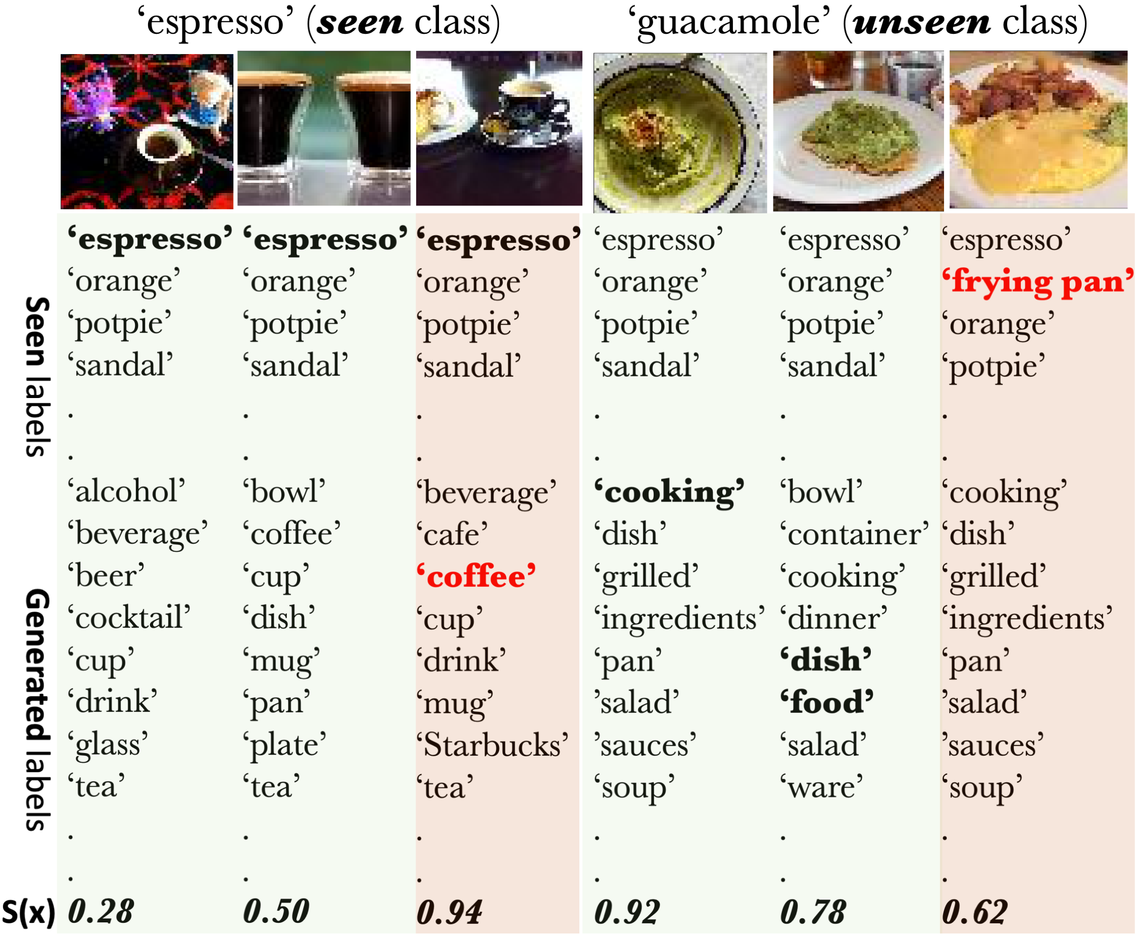
(a) Error study of generated labels

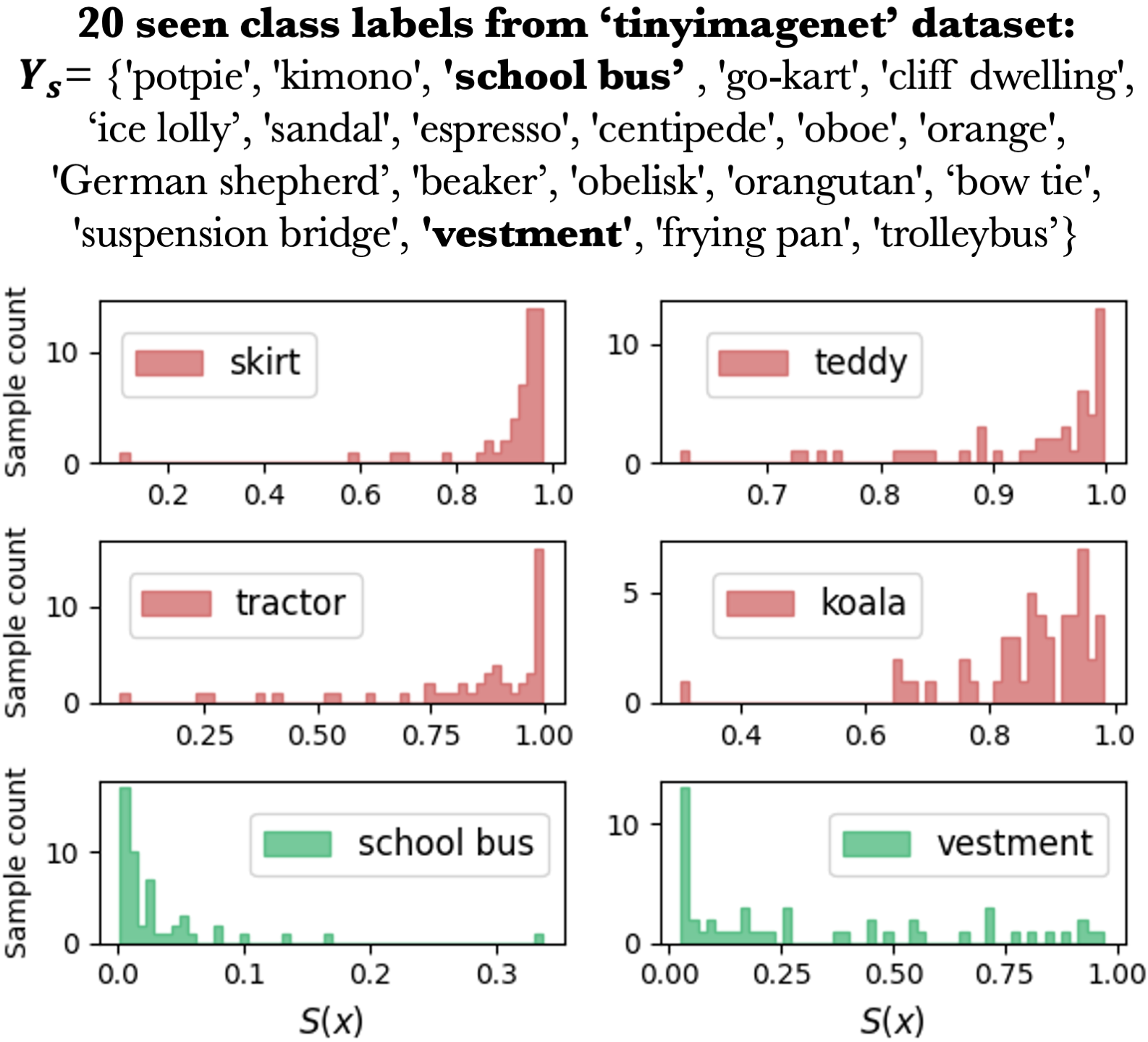
(b) Histograms of confidence scores

Figure 2: (a) A summary of the generated labels for a seen class ‘espresso’ and an unseen class ‘guacamole’ from the TinyImagenet dataset are shown. The generated labels are ranked based on their contribution to $S(x)$. The labels with ($P(y|x)>0.1$) are in boldface. For class ‘espresso’, we expect the model to output a relatively low $S(x)$ as the actual label is present among seen labels (first two images). The third image is an error case. The set of generated labels and the label ‘coffee’ produce a high $S(x)$. For the unseen class ‘guacamole’, $S(x)$ is high for the first two images as expected since ZOC correctly associates the generated labels with the images. The third image is again an error case when a seen label ‘frying pan’ contributes to $S(x)$ more than the generated unseen labels. (Best viewed in color) (b) 20 seen labels form tinyimagenet are listed at the top. 4 classes ‘skirt’, ‘teddy’, ‘tractor’ and ‘koala’ are a subset of unseen classes. Each subplot shows the histogram of the confidence score $S(x)$. For instance, in the histogram for unseen class ‘skirt’, we can clearly see that more than 40 samples have confidence scores between 0.8 and 1 which is desirable for good detection performance. S(x) tends to have a higher variance for the other 3 unseen class plots. It is interesting to note that for the samples from class ‘tractor’, the confidence score is relatively low because it is confused with semantically similar seen labels ‘school bus’ and ‘go-kart’. Similarly, low $S(x)$ for ‘koala’ mostly happen when the model associates the image with seen labels ‘orangutan’ and ‘German shepherd’. The confidence score for two seen classes ‘school bus’ and ‘vestment’ is distributed in lower ranges as expected. (Best viewed in color)

The experimental results are summarized in Table 1. We use AUROC (Area Under the ROC curve) as the evaluation measure as it is the most commonly used measure for OOD detection. ZOC outperforms all baselines by a large margin. A significant difference between ZOC and the baselines is that ZOC inference is based on dynamically generated candidate unseen labels for each sample, which gives ZOC a better detection capability.

Since ZOC uses CLIP’s pre-trained encoder for inference, one might attribute the performance gain to the rich feature space of CLIP. To investigate the gain, we set up an experiment with MSP (Hendrycks and Gimpel 2016) for CLIP. As mentioned earlier, MSP uses the maximum softmax score of zero-shot CLIP as the OOD confidence score. This experimental setup assesses CLIP’s inherent ability for OOD detection compared to ZOC’s inference technique. ZOC’s consistent performance gain over MSP on all datasets (Table 1) confirms that the proposed confidence score based on dynamic generation of unseen labels is better than MSP which uses identical inference procedure for all samples.

Note that we do not have an ablation study on ZOC as no part of the algorithm can be dropped for it to function.

Case study and error analysis.

Figure 2(a) is a case study illustrating the actual seen and candidate unseen labels (generated for each sample) used in calculating the confidence score $S(x)$. We picked one seen and one unseen class for comparison. Note that the actual label for a given image might/might not be among the generated labels. Particularly, this can happen when the unseen label is fine-grained and not present in the training corpus of MS-COCO. As a result, for an image with label ‘espresso’, the decoder generates relevant words such as ‘coffee’ rather than the label ‘espresso’ itself. Nevertheless, ZOC comes to the correct conclusion based on accumulative confidence score $S(x)$. Figure 2(b) illustrates the statistics of the calculated confidence score for 4 unseen and 2 seen classes from tinyimagenet. We plan to use a larger corpus to train the image description generator in the future. In addition, since ZOC compares standalone candidate labels to the image, it does not account for relations between the unseen labels. Such relations might be an important tool for detecting more sophisticated OOD samples. We will address this limitation in our future work.

Conclusion

In this paper, we introduced the new task of zero-shot OOD detection based on the recent advances in zero-shot closed-world classification using the pre-trained model CLIP (Radford et al. 2021). Since it is a zero-shot problem, 1) no concrete samples are given for training except the known or seen class label names, and 2) samples from unseen OOD classes may appear at the test time. To solve the problem, we extended the CLIP model so that it can dynamically generate candidate unseen labels for each test image, and also defined a novel confidence score calculated based on the similarity of the test image to seen and generated candidate unseen labels in the feature space. Experimental results confirmed that the proposed system ZOC is superior to the traditional supervised models. In addition, it also outperforms the baselines which use pre-trained CLIP backbone as their encoders.

References

- Andrews, Morton, and Griffin (2016) Andrews, J. T.; Morton, E. J.; and Griffin, L. D. 2016. Detecting anomalous data using auto-encoders. International Journal of Machine Learning and Computing, 6(1): 21.
- Bendale and Boult (2016) Bendale, A.; and Boult, T. E. 2016. Towards open set deep networks. In Proceedings of the IEEE conference on computer vision and pattern recognition, 1563–1572.
- Bengio et al. (2015) Bengio, S.; Vinyals, O.; Jaitly, N.; and Shazeer, N. 2015. Scheduled sampling for sequence prediction with recurrent neural networks. arXiv preprint arXiv:1506.03099.
- Chen et al. (2017) Chen, J.; Sathe, S.; Aggarwal, C.; and Turaga, D. 2017. Outlier detection with autoencoder ensembles. In Proceedings of the 2017 SIAM international conference on data mining, 90–98. SIAM.
- Devlin et al. (2018) Devlin, J.; Chang, M.-W.; Lee, K.; and Toutanova, K. 2018. Bert: Pre-training of deep bidirectional transformers for language understanding. arXiv preprint arXiv:1810.04805.
- Dosovitskiy et al. (2020) Dosovitskiy, A.; Beyer, L.; Kolesnikov, A.; Weissenborn, D.; Zhai, X.; Unterthiner, T.; Dehghani, M.; Minderer, M.; Heigold, G.; Gelly, S.; et al. 2020. An image is worth 16x16 words: Transformers for image recognition at scale. arXiv preprint arXiv:2010.11929.
- Fan, Lewis, and Dauphin (2018) Fan, A.; Lewis, M.; and Dauphin, Y. 2018. Hierarchical neural story generation. arXiv preprint arXiv:1805.04833.
- Fei and Liu (2016) Fei, G.; and Liu, B. 2016. Breaking the closed world assumption in text classification. In Proceedings of the 2016 Conference of the North American Chapter of the Association for Computational Linguistics: Human Language Technologies (NAACL-2016, 506–514.
- Fort, Ren, and Lakshminarayanan (2021) Fort, S.; Ren, J.; and Lakshminarayanan, B. 2021. Exploring the Limits of Out-of-Distribution Detection. arXiv preprint arXiv:2106.03004.
- Ge et al. (2017) Ge, Z.; Demyanov, S.; Chen, Z.; and Garnavi, R. 2017. Generative openmax for multi-class open set classification. arXiv preprint arXiv:1707.07418.
- He et al. (2016) He, K.; Zhang, X.; Ren, S.; and Sun, J. 2016. Deep residual learning for image recognition. In Proceedings of the IEEE conference on computer vision and pattern recognition, 770–778.
- Hendrycks and Gimpel (2016) Hendrycks, D.; and Gimpel, K. 2016. A baseline for detecting misclassified and out-of-distribution examples in neural networks. arXiv preprint arXiv:1610.02136.
- Hendrycks et al. (2020) Hendrycks, D.; Liu, X.; Wallace, E.; Dziedzic, A.; Krishnan, R.; and Song, D. 2020. Pretrained transformers improve out-of-distribution robustness. arXiv preprint arXiv:2004.06100.
- Hendrycks, Mazeika, and Dietterich (2018) Hendrycks, D.; Mazeika, M.; and Dietterich, T. 2018. Deep anomaly detection with outlier exposure. arXiv preprint arXiv:1812.04606.
- Holtzman et al. (2019) Holtzman, A.; Buys, J.; Du, L.; Forbes, M.; and Choi, Y. 2019. The curious case of neural text degeneration. arXiv preprint arXiv:1904.09751.
- Hsu et al. (2020) Hsu, Y.-C.; Shen, Y.; Jin, H.; and Kira, Z. 2020. Generalized odin: Detecting out-of-distribution image without learning from out-of-distribution data. In Proceedings of the IEEE/CVF Conference on Computer Vision and Pattern Recognition, 10951–10960.
- Kingma and Ba (2017) Kingma, D. P.; and Ba, J. 2017. Adam: A Method for Stochastic Optimization. arXiv:1412.6980.
- Krizhevsky, Hinton et al. (2009) Krizhevsky, A.; Hinton, G.; et al. 2009. Learning multiple layers of features from tiny images. Technical report, University of Toronto.
- Lamb et al. (2016) Lamb, A. M.; Goyal, A. G. A. P.; Zhang, Y.; Zhang, S.; Courville, A. C.; and Bengio, Y. 2016. Professor forcing: A new algorithm for training recurrent networks. In Advances in neural information processing systems, 4601–4609.
- Le and Yang (2015) Le, Y.; and Yang, X. 2015. Tiny imagenet visual recognition challenge. CS 231N, 7(7): 3.
- Lee et al. (2017) Lee, K.; Lee, H.; Lee, K.; and Shin, J. 2017. Training confidence-calibrated classifiers for detecting out-of-distribution samples. arXiv preprint arXiv:1711.09325.
- Lee et al. (2018) Lee, K.; Lee, K.; Lee, H.; and Shin, J. 2018. A simple unified framework for detecting out-of-distribution samples and adversarial attacks. Advances in neural information processing systems, 31.
- Liang, Li, and Srikant (2017) Liang, S.; Li, Y.; and Srikant, R. 2017. Enhancing the reliability of out-of-distribution image detection in neural networks. arXiv preprint arXiv:1706.02690.
- Lin et al. (2014) Lin, T.-Y.; Maire, M.; Belongie, S.; Hays, J.; Perona, P.; Ramanan, D.; Dollár, P.; and Zitnick, C. L. 2014. Microsoft coco: Common objects in context. In European conference on computer vision, 740–755. Springer.
- Miller et al. (2021) Miller, D.; Sunderhauf, N.; Milford, M.; and Dayoub, F. 2021. Class Anchor Clustering: A Loss for Distance-Based Open Set Recognition. In Proceedings of the IEEE/CVF Winter Conference on Applications of Computer Vision, 3570–3578.
- Neal et al. (2018) Neal, L.; Olson, M.; Fern, X.; Wong, W.-K.; and Li, F. 2018. Open set learning with counterfactual images. In Proceedings of the European Conference on Computer Vision (ECCV), 613–628.
- Oza and Patel (2019) Oza, P.; and Patel, V. M. 2019. C2ae: Class conditioned auto-encoder for open-set recognition. In Proceedings of the IEEE/CVF Conference on Computer Vision and Pattern Recognition, 2307–2316.
- Perera et al. (2020) Perera, P.; Morariu, V. I.; Jain, R.; Manjunatha, V.; Wigington, C.; Ordonez, V.; and Patel, V. M. 2020. Generative-discriminative feature representations for open-set recognition. In Proceedings of the IEEE/CVF Conference on Computer Vision and Pattern Recognition, 11814–11823.
- Pernici et al. (2018) Pernici, F.; Bartoli, F.; Bruni, M.; and Del Bimbo, A. 2018. Memory based online learning of deep representations from video streams. In Proceedings of the IEEE Conference on Computer Vision and Pattern Recognition, 2324–2334.
- Radford et al. (2021) Radford, A.; Kim, J. W.; Hallacy, C.; Ramesh, A.; Goh, G.; Agarwal, S.; Sastry, G.; Askell, A.; Mishkin, P.; Clark, J.; et al. 2021. Learning transferable visual models from natural language supervision. arXiv preprint arXiv:2103.00020.
- Rennie et al. (2017) Rennie, S. J.; Marcheret, E.; Mroueh, Y.; Ross, J.; and Goel, V. 2017. Self-critical sequence training for image captioning. In Proceedings of the IEEE conference on computer vision and pattern recognition, 7008–7024.
- Scheirer et al. (2012) Scheirer, W. J.; de Rezende Rocha, A.; Sapkota, A.; and Boult, T. E. 2012. Toward open set recognition. IEEE transactions on pattern analysis and machine intelligence, 35(7): 1757–1772.
- Scheirer, Jain, and Boult (2014) Scheirer, W. J.; Jain, L. P.; and Boult, T. E. 2014. Probability models for open set recognition. IEEE transactions on pattern analysis and machine intelligence, 36(11): 2317–2324.
- Shu et al. (2021) Shu, L.; Benajiba, Y.; Mansour, S.; and Zhang, Y. 2021. ODIST: Open World Classification via Distributionally Shifted Instances. In Findings of the Association for Computational Linguistics: EMNLP 2021, 3751–3756.
- Shu, Xu, and Liu (2017) Shu, L.; Xu, H.; and Liu, B. 2017. Doc: Deep open classification of text documents. Proceedings of the 2017 Conference on Empirical Methods in Natural Language Processing, EMNLP 2017.
- Shu, Xu, and Liu (2018) Shu, L.; Xu, H.; and Liu, B. 2018. Unseen class discovery in open-world classification. arXiv preprint arXiv:1801.05609.
- Tack et al. (2020) Tack, J.; Mo, S.; Jeong, J.; and Shin, J. 2020. Csi: Novelty detection via contrastive learning on distributionally shifted instances. arXiv preprint arXiv:2007.08176.
- Vaswani et al. (2017) Vaswani, A.; Shazeer, N.; Parmar, N.; Uszkoreit, J.; Jones, L.; Gomez, A. N.; Kaiser, Ł.; and Polosukhin, I. 2017. Attention is all you need. In Advances in neural information processing systems, 5998–6008.
- Williams and Zipser (1989) Williams, R. J.; and Zipser, D. 1989. A learning algorithm for continually running fully recurrent neural networks. Neural computation, 1(2): 270–280.
- Winkens et al. (2020) Winkens, J.; Bunel, R.; Roy, A. G.; Stanforth, R.; Natarajan, V.; Ledsam, J. R.; MacWilliams, P.; Kohli, P.; Karthikesalingam, A.; Kohl, S.; et al. 2020. Contrastive training for improved out-of-distribution detection. arXiv preprint arXiv:2007.05566.
- Wolf et al. (2020) Wolf, T.; Debut, L.; Sanh, V.; Chaumond, J.; Delangue, C.; Moi, A.; Cistac, P.; Rault, T.; Louf, R.; Funtowicz, M.; Davison, J.; Shleifer, S.; von Platen, P.; Ma, C.; Jernite, Y.; Plu, J.; Xu, C.; Scao, T. L.; Gugger, S.; Drame, M.; Lhoest, Q.; and Rush, A. M. 2020. Transformers: State-of-the-Art Natural Language Processing. In Proceedings of the 2020 Conference on Empirical Methods in Natural Language Processing: System Demonstrations, 38–45. Online: Association for Computational Linguistics.
- Xu et al. (2019) Xu, H.; Liu, B.; Shu, L.; and Yu, P. 2019. Open-world learning and application to product classification. In The World Wide Web Conference, 3413–3419.