Magnetic loading of magnetars’ flares

Abstract

Magnetars, the likely sources of Fast Radio Bursts (FRBs), produce both steady highly relativistic magnetized winds, and occasional ejection events. We demonstrate that the requirement of conservation of the magnetic flux dominates the overall dynamics of magnetic explosions. This is missed in conventional hydrodynamic models of the ejections as expanding shell with parametrically added magnetic field, as well as one-dimensional models of magnetic disturbances. Most of the initial free energy of an explosion is actually spent on stretching its own internal magnetic field, while doing minimal $pdV$ work against the surrounding. Magnetic explosions from magnetars come into force balance with the pre-flare wind close to the light cylinder. They are then advected quietly with the wind, or propagate as electromagnetic disturbances. No powerful shock waves are generated in the wind.

1 Introduction

Observations of correlated radio and X-ray bursts (CHIME/FRB Collaboration et al., 2020; Ridnaia et al., 2020; Bochenek et al., 2020; Mereghetti et al., 2020; Li et al., 2021) established the FRB-magnetar connection.

Two kind of models of FRBs’ loci are competing at the moment. The first advocates that FRBs are magnetospheric events, e.g.  Solar flare-like (Lyutikov, 2002b, 2006b, 2006a; Lyutikov & Popov, 2020; Lyubarsky, 2020); the emission mechanism remains unidentified, akin to the 50+ years problem of pulsar radio emission (see Lyubarsky, 2020; Lyutikov, 2021, for new ideas). Second are wind-generated GRB-like events (Lyubarsky, 2014; Beloborodov, 2017; Metzger et al., 2019, 2017, 2019; Beloborodov, 2020). Emission mechanism is the cyclotron maser (Gallant & Arons, 1994; Plotnikov & Sironi, 2019; Babul & Sironi, 2020). (For discussion of general constraints on plasma parameters and models see e.g.  Lyutikov & Rafat, 2019; Lyubarsky, 2021)

In this paper we argue that wind-model of FBRs are internally inconsistent. Qualitatively, these models use the hydrodynamic paradigm of the internal shocks models of GRBs, the flying shells (Piran, 2004), with parametrically added magnetic field component. This simple addition of magnetic field cannot be applied in principle to the magnetic explosions of magnetars. The key point is the conservation of the magnetic flux within the exploding plasma. This is related to the sigma-problem in pulsar winds (Rees & Gunn, 1974; Kennel & Coroniti, 1984), reformulated by Lyutikov & Blandford (2003); Lyutikov (2006c) as a magnetic flux conservation problem. The theoretical difference between the two model (the “magnetized shells” and the present model), are enormous. Instead of highly relativistic shock with the Lorentz factor over a million, as advocated by e.g.  Beloborodov (2020), the magnetic explosions comes into a force balance approximately near the light cylinder, and propagates as an electromagnetic pulse there on. No powerful shocks are generated. Hence no emission of FRBs from the far wind.

We first give an analysis of the wind-FRB models (Metzger et al., 2019; Beloborodov, 2020) from the point of basic theory of pulsar winds and relativistic shock propagating through the winds, §2. These are the types of “double relativistic explosion” previously considered in various set-up by Lyutikov (2002a, 2011a, 2017); Lyutikov & Camilo Jaramillo (2017); Barkov et al. (2021). In the main §3 we argue that an effective “magnetic loading” quickly reduces the power of the magnetar’s explosion, producing either an EM pulse through the wind, or a confined magnetic structure in pressure balance with the wind. No ultra-relativistic shocks are produced.

2 The pulsar wind and shock dynamics in the magnetized wind

2.1 Pulsar wind primer

Pulsar and magnetars produce relativistic highly magnetized winds (Michel, 1969; Goldreich & Julian, 1970; Michel, 1973), that can be parametrized by the wind luminosity $L_{w}$ and the ratio of Poynting to particle fluxes:

$$\mu_{w}=\frac{L_{w}}{\dot{N}m_{e}c^{2}}=\frac{B_{LC}^{2}}{4\pi n_{LC}m_{e}c^{2}}$$ (1)

where $\dot{N}$ is the rate of lepton ejection by the neutron star; subscript LC indicates values measured at the light cylinder,

$$R_{LC}=4\times 10^{9}\,P\,{\rm cm}$$ (2)

for the period of a star $P$ measured in seconds. Expected values of $\mu_{w}$ are in the range of $10^{4}-10^{6}$ (Arons & Scharlemann, 1979; Arons, 1983; Hibschman & Arons, 2001; Beloborodov & Thompson, 2007). In the case of GJ scaling of density, with multiplicity $\kappa=n/n_{GJ}$,

$$\dot{N}=\kappa\frac{\sqrt{cL_{w}}}{e}$$ (3)

Initially the wind accelerates linearly away from the light cylinder

$$\Gamma_{w}=\frac{r}{R_{LC}}$$ (4)

so that the wind magnetization decreases

$$n^{\prime}=\left(\frac{R_{LC}}{r}\right)^{-3}n_{LC}\mbox{}$$

$$B^{\prime}=\left(\frac{R_{LC}}{r}\right)^{-2}B_{LC}\mbox{}$$

$$\sigma(r)=\frac{B^{\prime,2}}{4\pi n^{\prime}m_{e}c^{2}}=\frac{R_{LC}}{r}\mu_{w}$$ (5)

(primes denote quantities measured in the wind frame.)

The terminal value for the wind acceleration is the Alfvén  condition,

$$\Gamma_{w}=\sigma_{w}^{1/2}=\mu_{w}^{1/3}\mbox{}$$

$$\sigma_{w}=\mu_{w}^{2/3}\gg 1$$ (6)

reached at

$$R_{w}=\mu_{w}^{1/3}R_{LC}=\Gamma_{w}R_{LC}$$ (7)

Total energy and mass (in lab frame) contained in the acceleration region,

$$E_{w}=L_{w}\frac{R_{w}}{c}\mbox{}$$

$$M_{w}=m_{e}\dot{N}\frac{R_{w}}{c}$$ (8)

are typically insignificant; mass loading of the following shock is further reduced by $1/\Gamma_{w}$.

At distances $r>R_{w}$

$$\Gamma_{w}=\mu_{w}^{1/3}\mbox{}$$

$$n^{\prime}=\mu^{-1/3}\left(\frac{R_{LC}}{r}\right)^{-2}n_{LC}\mbox{}$$

$$B^{\prime}=\mu^{-1/3}\left(\frac{R_{LC}}{r}\right)^{-1}B_{LC}\mbox{}$$

$$\sigma_{w}=\mu_{w}^{2/3}\mbox{}$$

$$\Gamma^{\ast}=2\sqrt{\sigma_{w}}\Gamma_{w}=2\mu_{w}^{2/3}=2\Gamma_{w}^{2}$$ (9)

Quantity $\Gamma^{\ast}$ is the Lorentz factor  (measured in lab frame) required to produce a shock in the receding wind.

The above considerations assumes no magnetic dissipation. At the basic level it is not consistent with observations of the PNWe. As Rees & Gunn (1974); Kennel & Coroniti (1984) argued, $\sigma_{w}$ cannot remain $\gg 1$ until the (conventional MHD) wind termination shock. It should drop to $\leq 10^{-2}$. This can happen either close to the LC Lyubarsky & Kirk (2001); Coroniti (1990) or at the termination shock (Lyubarsky, 2003; Sironi & Spitkovsky, 2009, 2011). As Porth et al. (2014) argued, magnetic dissipation can occur in the bulk of the nebula (Porth et al., 2017); still observations of the Crab’s Inner knot require that a large sector of the wind has low magnetization (Lyutikov et al., 2016). In the limit of dominant dissipation in the near wind, $\sigma_{w}\leq 1$, all of spin-down is carried by particle flow, hence in that case $\Gamma_{w}=\mu_{w}\sim 10^{4}-10^{6}$.

2.2 Explosions in relativistic winds

Let us next consider explosions in the preceding magnetar wind. We assume that some kind of the central engine (a magnetar) produces energetic events on top of the steady wind. This will constitute a type of double relativistic explosion (Lyutikov, 2002a, 2011a, 2017; Lyutikov & Camilo Jaramillo, 2017; Barkov et al., 2021). First, we solve a formal MHD problem, and then discuss its limitations.

2.2.1 Point explosion in relativistic fluid wind

Consider a relativistic fluid wind of luminosity $L_{w}$ moving with Lorentz factor $\Gamma_{w}$

$$L_{w}=4\pi r^{2}\Gamma_{w}^{2}n_{w}^{\prime}m_{e}c^{3}=\Gamma_{w}\dot{M}_{w}c^{2}$$ (10)

where $n_{w}^{\prime}$ is density in the wind frame; the lab frame density is $n_{w}=\Gamma_{w}n_{w}^{\prime}$.

Consider an explosion that involves energy $E_{ej}$ and no mass $M_{ej}=0$. Thus, we assume that the energy of the explosion is transferred to the wind instantaneously. Consider a shock moving with Lorentz factor $\Gamma\gg\Gamma_{w}$ (as measured in lab frame). In a shock frame typical energy of post-shock particles is $T_{2}\sim\Gamma/(2\Gamma_{w})$. The shock sweeps particles giving them bulk Lorentz factor $\Gamma$; at radius $r$ the swept-up mass (in lab frame) is $L_{w}r/(c^{2}\Gamma_{w})$. Thus

$$\Gamma\sim\sqrt{2}\Gamma_{w}\sqrt{\frac{R_{0}}{r}}$$ (11)

where

$$R_{0}=\frac{cE_{ej}}{L_{w}}$$ (12)

2.2.2 Point explosion in relativistic magnetized wind

Relativistic explosions in static magnetic configurations were studied by Lyutikov (2002a), producing self-similar solutions solutions of the kind of Blandford & McKee (1976). Let us generalize them to the moving media. Below we are not interested in the structure of the flow (it will be the same as found in Lyutikov, 2002a), but in the overall scaling of the shock Lorentz factor $\Gamma$ dependance on the wind parameters.

Let us first consider a simple, extreme case of point magnetospheric explosion with no mass loading. Let the wind preceding the ejection have magnetization $\sigma_{w}\gg 1$. Neglecting small contribution to the wind luminosity from the particles

$$L_{w}=4\pi r^{2}\Gamma_{w}^{2}\frac{B_{w}^{\prime,2}}{4\pi}c$$ (13)

Consider again an explosion that involves energy $E_{ej}$ and no mass $M_{ej}=0$. The interaction in the accelerating region $r\leq R_{w}$, before the wind reaches $\Gamma_{w}$, does not affect much the flow, because of small $E_{w}$ and $M_{w}$, high values of $\sigma(r)$ and the fact that both the ejecta and the wind accelerate linearly with $r$. (This statement has been verified according to the following discussion.)

Consider a shock moving with Lorentz factor $\Gamma$ (as measured in lab frame) through a highly magnetized wind, which itself is moving with $\Gamma_{w}$. Let the values of the magnetic field in the lab frame before the shock be $B_{w}$,

$$B_{w}=\frac{\sqrt{L_{w}}}{\sqrt{r}c}\mbox{}$$

$$B_{w}^{\prime}=\frac{B_{w}}{\Gamma_{w}}$$ (14)

(prime is in wind frame). The shock is moving through the wind with

$$\Gamma_{s}=\frac{\Gamma}{2\Gamma_{w}}$$ (15)

In the frame of the shock the shocked part of the wind moves with Lorentz factor $\sqrt{\sigma_{w}}$. It carries magnetic field

$$B_{2}^{\prime}=\frac{\Gamma}{2\Gamma_{w}\sqrt{\sigma_{w}}}B_{w}^{\prime}$$ (16)

as measured in the post-shock frame. The post shock frame moves with Lorentz factor $\Gamma/(2\sqrt{\sigma_{w}})$ in lab frame, thus

$$B_{w,2}=\left(\frac{\Gamma}{\Gamma^{\ast}}\right)^{2}B_{w}$$ (17)

This is magnetic field in the post shock region as measured in the lab frame.

The swept-up material is located within

$$\Delta r\sim\frac{\sigma}{\Gamma^{2}}r$$ (18)

The energy budget reads (particle contribution is neglected for $\sigma_{w}\gg 1$)

$$E_{ej}=c\left({B_{w,2}^{2}}\right)r^{2}\Delta r\approx{L_{w}r}\frac{\Gamma^{2}}{4\sigma_{w}\Gamma_{w}^{4}}$$ (19)

Thus,

$$\Gamma=2\Gamma_{w}^{2}\sqrt{\sigma_{w}}\sqrt{\frac{R_{0}}{r}}\to 2\sqrt{\frac{R_{0}}{r}}\Gamma_{w}^{3}$$ (20)

where the last relation assumed $\Gamma_{w}=\sqrt{\sigma_{w}}$. Notice the difference in the power of $\Gamma_{w}$ in comparison with the fluid case (11).

In observer time

$$t_{ob}=\frac{t}{2\Gamma^{2}}=\frac{ct^{2}}{8R_{0}\Gamma_{w}^{4}\sigma_{w}}\mbox{}$$

$$\Gamma=2^{1/4}\Gamma_{w}\sigma_{w}^{1/4}\left(\frac{R_{0}}{ct_{ob}}\right)^{1/4}$$ (21)

The energy is concentrated in

$$\frac{\Delta r}{r}=\frac{1}{8\Gamma_{w}^{4}}\frac{r}{R_{0}}$$ (22)

(independent of $\sigma_{w}$)

2.3 Shock interaction of relativistic winds

Let’s next assume that the first wind is followed by the second wind from the flare with Lorentz factor $\Gamma_{f}$, wind frame magnetic field $B_{f}$ and magnetization $\sigma_{f}$

$$L_{f}=\Gamma_{f}^{2}B_{f}^{2}r^{2}c$$ (23)

Assume strong interaction, so that a reverse shock (RS) is generated in the flare wind and forward shock (FS) is generated in pre-explosion wind. Let in the lab frame the contact discontinuity between two winds move with Lorentz factor $\Gamma_{CD}$. Then

$$\Gamma_{FS}=2\sqrt{\sigma_{w}}\Gamma_{CD}\mbox{}$$

$$\Gamma_{RS}=\frac{\Gamma_{CD}}{2\sqrt{\sigma_{f}}}$$ (24)

Lorentz factor of the RS with respect to the flare flow is

$$\Gamma_{RS}^{\prime}=\frac{\Gamma_{f}}{\Gamma_{CD}\sqrt{\sigma_{f}}}$$ (25)

Balancing magnetic field in the shocked wind and shocked flare flows

$$\frac{\Gamma_{CD}}{\Gamma_{w}^{2}}\frac{\sqrt{L_{w}}}{\sqrt{c}r}=\frac{1}{2\Gamma_{C}D}\frac{\sqrt{L_{f}}}{\sqrt{c}r},$$ (26)

we find

$$\Gamma_{CD}=\left(\frac{L_{f}}{L_{w}}\right)^{1/4}\Gamma_{w}\mbox{}$$

$$\Gamma_{FS}=2\left(\frac{L_{f}}{L_{w}}\right)^{1/4}\Gamma_{w}\sqrt{\sigma_{w}}\mbox{}$$

$$\Gamma_{RS}=\frac{1}{2}\left(\frac{L_{f}}{L_{w}}\right)^{1/4}\frac{\Gamma_{w}}{\sqrt{\sigma_{f}}}\mbox{}$$

$$\Gamma_{RS}^{\prime}=\left(\frac{L_{f}}{L_{w}}\right)^{1/4}\frac{\Gamma_{f}\sqrt{\sigma_{f}}}{\Gamma_{w}}$$ (27)

Strong shock conditions require that post-shock temperature are relativistic. For the forward shock

$$T_{FS}=\frac{1}{8\sqrt{\sigma_{w}}}\frac{\Gamma_{FS}}{2\Gamma_{w}}>1\to\frac{1}{8}\left(\frac{L_{f}}{L_{w}}\right)^{1/4}\mbox{}$$

$$L_{f}\geq 4\times 10^{3}L_{w}$$ (28)

For the reverse shock

$$T_{RS}=\frac{1}{8}\left(\frac{L_{f}}{L_{w}}\right)^{1/4}\frac{\Gamma_{f}}{\Gamma_{w}}\mbox{}$$

$$\Gamma_{f}\geq 8\left(\frac{L_{f}}{L_{w}}\right)^{1/4}\Gamma_{w}$$ (29)

Curiously, the fraction of the flare-wind $\eta_{RS}$ used to push the magnetar wind increases with its magnetization

$$\eta_{RS}\sim\frac{1}{\Gamma_{RS}^{2}}=4\left(\frac{L_{w}}{L_{f}}\right)^{1/2}\frac{\sigma_{f}}{\Gamma_{w}^{2}}$$ (30)

This is because for higher $\sigma_{f}$ the RS moves faster through the flare wind ($\eta_{R}$ is not the dissipated power that is put into particles, that one is smaller by $\Gamma_{RS}^{\prime}/(8\sqrt{\sigma_{f}})$).

The main constraint for the wind-wind interaction comes from the fact that the flare wind should be supersonic with respect to the magnetar wind. To make a shock in the preceding wind it is required that

$$\Gamma_{f}>\Gamma^{\ast}=2\Gamma_{w}\sqrt{\sigma_{w}}=2\Gamma_{w}^{2}$$ (31)

Since acceleration of the flare proceed according to the same law (7), this requires

$$\Gamma_{f}=\sqrt{\sigma_{f}}\mbox{}$$

$$\sigma_{f}\geq 4\Gamma_{w}^{4}$$ (32)

Since terminal magnetization is related to the parameter $\mu_{w}$ by (9), it is required that

$$\mu_{f}=\sigma_{f}^{3/2}=8\Gamma_{w}^{6}$$ (33)

Thus the flare wind must be much cleaner than the initial wind

$$\frac{\mu_{f}}{\mu_{w}}>8\Gamma_{w}^{4}$$ (34)

2.4 The fluid engine

Above we took an extreme position, that the energy transfer from the ejecta to the wind was instantaneous, zero mass and zero magnetic loading at the explosion site. In fact, energy transfer between two relativistically expanding and relativistically accelerating flows will be inefficient. Two factors are at play. First, there is a problem with creation of shocks during the acceleration stage of the wind: in the acceleration region the magnetization is extremely high, Eq. (5). It is very hard to create a shock in a highly magnetized flow. Consider for example a fluid explosion starting with ejection at $R_{ej}\leq R_{LC}$. Acceleration of the fluid ejecta is linear at first (Paczynski, 1986)

$$\Gamma_{ej}=\frac{r}{R_{ej}}$$ (35)

At the wind acceleration stage $r<R_{w}$, the condition that the ejecta makes a strong shock in the preceding wind is (see Eq. (5)

$$\Gamma_{ej}\geq 2\sqrt{\sigma(r)}\Gamma(r)=2\mu_{w}^{1/2}\sqrt{\frac{r}{r_{LC}}}$$ (36)

This requires

$$\frac{r}{R_{LC}}\geq(256\mu_{w})\left(\frac{R_{ej}}{R_{LC}}\right)^{2}$$ (37)

Since $\mu\gg 1$, the fluid ejecta just starts to make a shock at large distances.

Second, shock or not, if there is an over-pressurized region with energy density $u$ in the lab frame, which is expanding with Lorentz factor $\Gamma$, then the energy density in the frame associated with the interface of the two interacting media is $\sim u/\Gamma^{2}$. This is the force per unit area that contributes to the acceleration of a lower-pressure region. The acceleration time (energy transfer time) in the lab frame $t_{acc}$ is slower by another factor of $\Gamma$, hence the shortest time to transfer energy from the ejecta to the previous wind is $t_{acc}\sim\Gamma^{3}(r/c)$. For example if interaction starts at $R_{w}\sim\Gamma_{w}R_{LC}$ (7), the energy transfer time is $\sim\Gamma_{w}^{4}R_{LC}$.

3 Magnetically-driven explosions

3.1 Not “magnetic shells”

Above we summarized the dynamics of magnetized shocks in magnetized winds. We did not address in details the energy release process, just highlighted in §2.4 possible issues with the fluid engine. The early dynamics is the key. As we are interested in magnetic explosions from highly magnetized magnetar, the engine and the explosion are both magnetic.

Typically magnetic explosions were considered in a framework of the internal shock model of GRB (Piran, 2004), as analogue of flying fluid shells (e.g.  Beloborodov, 2020), but with internal magnetic field. This is not correct in principle: dynamics of magnetic explosions cannot be reduced to “magnetized shells”.

First, in the case of one-dimensional magnetic explosion Lyutikov (2010) found a fully analytic one-dimensional solution, a simple wave, for a non-stationary expansion of high magnetized plasma into vacuum and/or low density medium. The result is somewhat surprising: initially the plasma accelerates as $\Gamma\propto t^{1/3}$ and can reach terminal Lorentz factor $\Gamma_{f}=1+2\mu_{0}$. where $\mu_{0}$ is the initial magnetization (see also Levinson, 2010). Thus, it was shown, that time-dependent explosions can achieve much larger Lorentz factors that the steady state flows: $2\mu_{0}$ for non-steady versus $\mu_{0}^{1/3}$ for steady-state (in this particular application $\mu_{0}=\sigma_{0}$). The force-free solution were generalized to the MHD regime (using a mathematically tricky hodograph transformation by Lyutikov & Hadden, 2012).

Importantly, those were specifically one-dimensional models of local break-out of magnetized jet from, e.g.  a confining star in GRB outflows. They cannot be simply used to describe fully three-dimensional magnetic explosions. What is different in multidimensional magnetic explosions is the conservation of the magnetic flux. Such issues does not appear for one-dimensional motion.

As Rees & Gunn (1974); Kennel & Coroniti (1984) argued, the presence of the global magnetic field changes the dynamics completely if compared with the fluid case. Lyutikov & Blandford (2003); Lyutikov (2006c) reformulated the problem in terms of the magnetic flux: the $\sigma$-problem is the problem of the (properly defined) toroidal magnetic flux conservation. Below we apply those ideas to the launching region of magnetic explosions.

3.2 Dynamics of magnetic explosion

Let’s assume that a magnetospheric process (e.g.  flare-like event) created a magnetic bubble, disconnected from the rest of the magnetosphere. The bubble contains both toroidal and poloidal magnetic flux, Fig. 2.

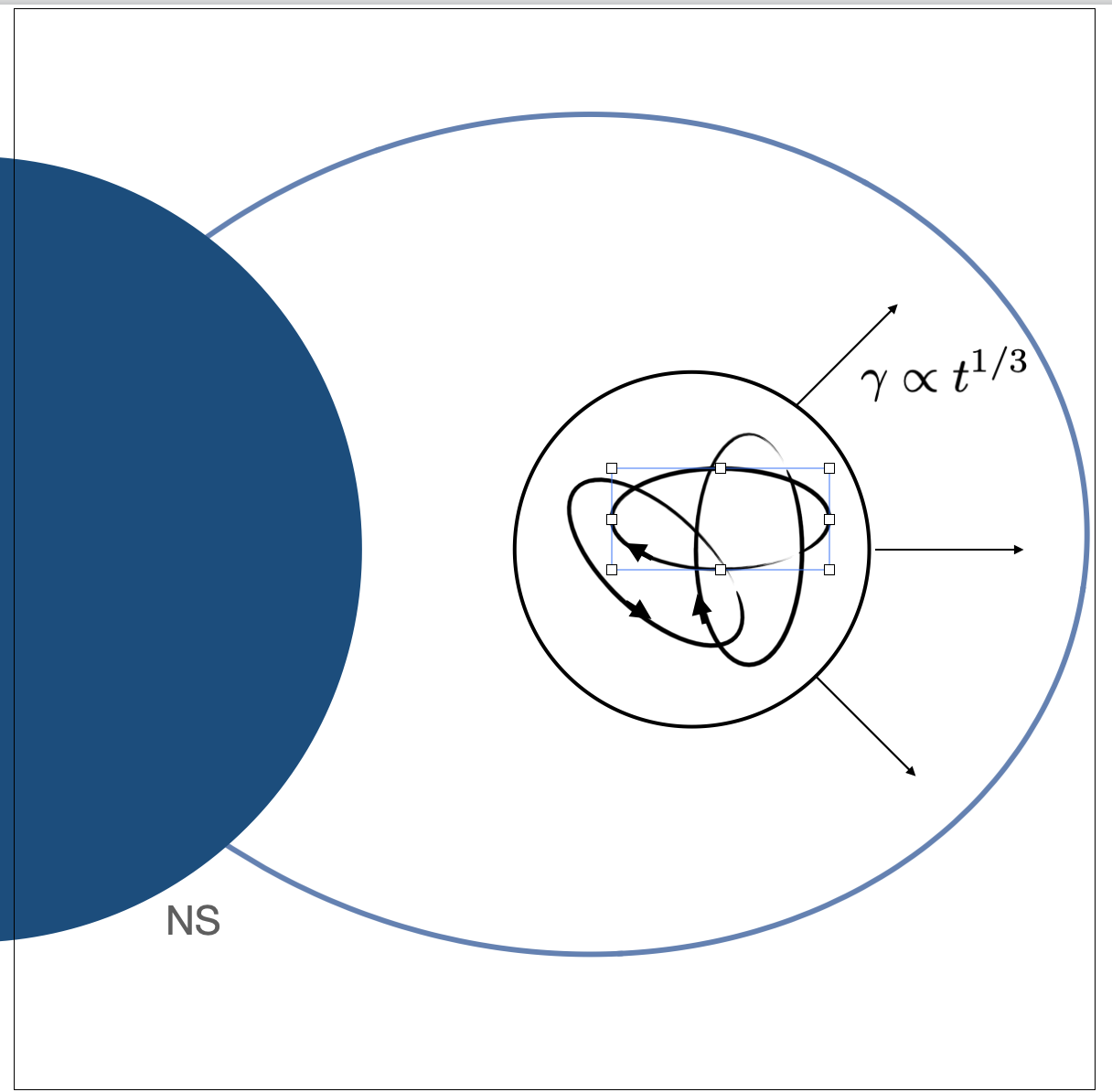
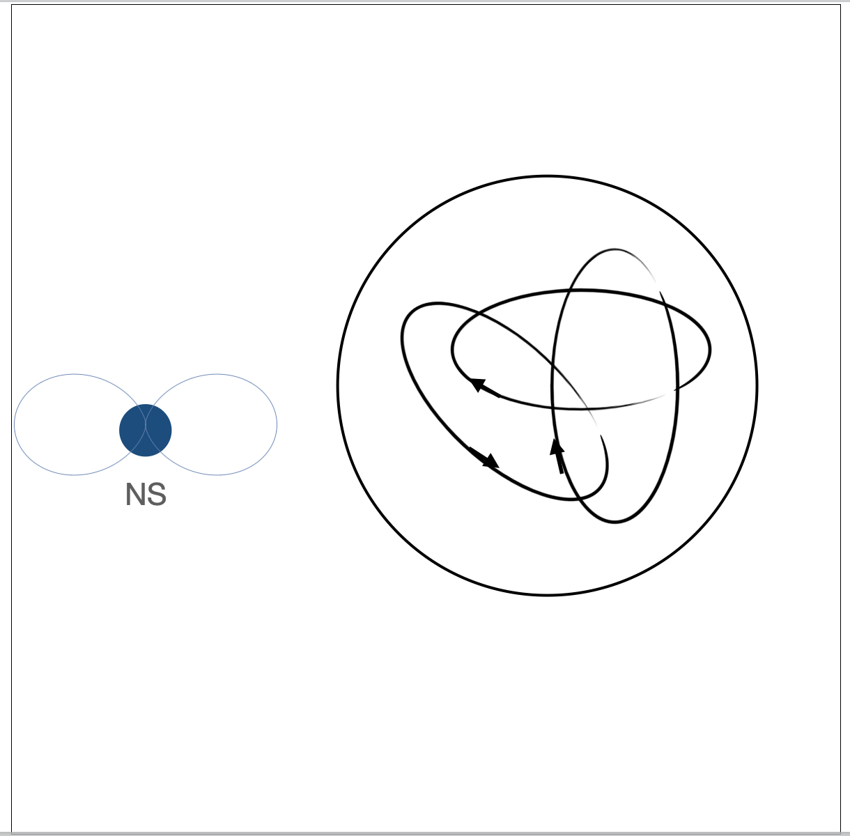
Figure 1: Cartoon of magnetic explosion. Left panel: a Solar flare-type even near the surface of the neutron star produces a magnetically disconnected magnetized cloud with complicated (linked) internal magnetic structure and total internal pressure (magnetic field and pairs) slightly exceeding the local dipole field. As the magnetic blob expands its pressure quickly becomes larger than of the surrounding dipolar one. Expansion quickly becomes relativistic. Later on, as the blob expands, magnetic field in the blob scales as $B_{b}\sim 1/R^{2}$, much faster the magnetic field in the wind. As a result, the expelled blob quickly reaches pressure equipartition with the wind flow.

The strong gradient of the dipolar field will push the magnetic bubble away. It will quickly become highly over-pressurized, and will start expanding. The expansion will have two stage. First, near the surface of the bubble the field is purely tangential. At this stage expansion is described by the 1D model of Lyutikov (2010). If initial magnetization within the bubble was $\sigma_{0}$, the flow becomes supersonic at the moment the expansion reaches $\Gamma=(\sigma_{0}/2)^{1/3}$. Unlike the stationary wind when acceleration ends at the sonic point, non-stationary magnetic explosion continues to accelerate to $\Gamma=1+2\sigma_{0}$.

After a rarefaction wave propagated deep inside the magnetic bubble, the expansion dynamics changes. The bubble consists of closed magnetic loops. Flux conservation requires that the magnetic field with the bubble scales as $B\propto 1/R^{2}$, where $R$ is a current size of the bubble. As long as the expelled blob is inside the light cylinder, the dipolar field decays much faster $\propto 1/R^{3}$ (the bubble is also moving away from the star, so it is located approximately at a distance $R$ comparable to its size), so the expansion of the blob occurs almost like in vacuum. The energy contained within a blob decreases $E\sim B^{2}R^{4}\propto R^{-1}$. When the size of the expanding bubble becomes larger than the light cylinder, the external magnetic field change its scaling from $\propto R^{-3}$ to $\propto R^{-1}$. Thus, the bubble quickly reaches equipartition with the wind field.

For example, if the bubble is created near the neutron star with typical energy

$$E_{f}\sim B_{f}^{2}R_{f}^{3}$$ (38)

The magnetic field inside the newly created magnetic cloud is of the order of the NS’s surface field $B_{NS}$, $B_{f}\sim B_{NS}$, and a size smaller than $R_{NS}$, $R_{f}=\eta_{R}R_{NS}$, $\eta_{R}\ll 1$. (Only giant flares need $\eta_{R}\sim 1$, FRBs with nearly quantum magnetic field need about a football field of energy to account for the high energy emission, $\eta_{R}\sim 10^{-2}$, see §3.6.) So,

$$E_{f}\sim\eta_{R}^{3}B_{NS}^{2}R_{NS}^{3}$$ (39)

Given the $\propto 1/R^{2}$ decrease of the magnetic field within the bubble, the pressure balance between the expanding flux tube and the wind at $r\geq R_{LC}$ gives the radius $R_{eq}$ when the expanding flux tubes reaches the force balance with the wind

$$\frac{R_{eq}}{R_{LC}}=\eta_{R}^{3/2}\frac{R_{LC}}{R_{NS}}$$ (40)

Since the $\eta_{R}\ll 1$, this is achieved fairly close to the light cylinder.

At larger distances the bubble is just advected with the wind, always kept at the force balance on the surface. The light bubble is also first accelerated with the wind, and then coasts (at $r>R_{w}$). Since in the coasting stage the confining magnetic field decreases as $1/r$, the size of the bubble increases as $R_{bubble}\propto r^{1/2}$. Eventually, when the magnetar’s wind starts interacting with the ISM, the ejected bubble shocks the ISM and produces radio afterglow (Cameron et al., 2005; Gaensler et al., 2005) seen after the giant flare of SGR 1806-20 (Palmer et al., 2005; Hurley et al., 2005), as described by Mehta et al. (2021)

3.3 Where did all the energy go? - Magnetic loading

We seem to run into a little paradox. In the case of FRBs the newly created magnetic bubble with energy (39) would have more energy than the energy of the magnetic field measured at the light cylinder, within the volume of a light cylinder,

$$E_{f}\gg E_{LC}\sim\frac{B_{NS}^{2}R_{NS}^{6}}{R_{LC}^{3}}$$ (41)

Yet, the expanding bubble came into force-balance with the preceding wind near the light cylinder. Where did the extra energy go?

It went into the stretching of the internal magnetic field of the bubble. Recall that the pressure of the magnetic field along the field is negative: the fields “wants” to contract. Stretching the field (expanding loops of the tangled magnetic field) requires work to be done against the contracting parallel force. The over-pressurized magnetically-dominated configuration “forces” the field to expand, thus making work on the internal field. As a result, most of the excess magnetic energy is spent on stretching the internal magnetic field, not on producing shocks/making $pdV$ work on the surrounding medium. This effect can be called a magnetic loading.

We come to an important conclusion: magnetic explosions are dominated not by the mass loading, but by the magnetic loading. Even very powerful explosion, with energies much larger than $B_{LC}^{2}R_{LC}^{3}$ reach a force balance close to the light cylinder. After that they are locked in the flow, and quietly advected.

3.4 Expanding spheromak/flux ropes

To illustrate the above points with the fully analytical model, and suggest possible variations, one can assume that a newly created bubble resembles a spheromak Bellan (2000). A possible model of the newly created magnetic cloud is a slightly over-pressured spheromak, Fig. 2.

We can appeal then to the fully analytical solution for non-relativistically expanding spheromak Lyutikov & Gourgouliatos (2011):

$$B_{r}=2B_{0}\alpha{j_{1}\over\alpha_{0}^{2}r}\cos\theta,\mbox{}$$

$$B_{\theta}=-B_{0}\alpha{j_{1}+\alpha rj_{1}^{\prime}\over\alpha_{0}^{2}r}\sin\theta,\mbox{}$$

$$B_{\phi}=B_{0}j_{1}\left({\alpha\over\alpha_{0}}\right)^{2}\sin\theta,\mbox{}$$

$$E_{r}=0,\mbox{}$$

$$E_{\theta}=-B_{0}{\alpha\dot{\alpha}\over\alpha_{0}^{2}}rj_{1}\sin\theta=-B_{\phi}{\dot{\alpha}\over\alpha}r,\mbox{}$$

$$E_{\phi}=-B_{0}\dot{\alpha}{j_{1}+\alpha rj_{1}^{\prime}\over\alpha_{0}^{2}}\sin\theta=B_{\theta}{\dot{\alpha}\over\alpha}r,\mbox{}$$

$${\bf E}=\left({\dot{\alpha}\over\alpha}r\right){\bf e}_{r}\times{\bf B}.$$ (42)

where $j_{1}$ is a Bessel function, $\alpha_{0}\sim 1/R_{0}$ is the initial radius, $\alpha\sim 1/R$ is the current radius. The total magnetic helicity, ${\cal H}=\int dV{\bf B}\cdot{\bf A}=1.4\times 10^{-2}B_{0}^{2}R_{0}^{4}$, as well as the toroidal magnetic flux ${\cal F}=\int B_{\phi}rdr=5.26B_{0}R_{0}^{2}$ are constant. Importantly, note: $B\propto 1/R^{2}$.

The total energy of the expanding spheromak

$$E_{\rm tot}=\int dV{E^{2}+B^{2}\over 8\pi}\propto{B_{0}^{2}R_{0}^{4}\over R}$$ (43)

decreases. This is a fully analytical solution illustrating the principal points made in §3.2.

The late expansion of a spheromak will be somewhat different though. On the surface the magnetic field of the spheromak scales as $B_{\perp}\propto\sin\theta$. Thus, initial expansion will be mostly equatorial. The expanding part of the spheromak, with high toroidal magnetic field, becomes causally disconnected and forms an expanding magnetic flux tube, right panel in Fig. 2 (Lyutikov & Gourgouliatos, 2011, also discussed the expanding flux rope, though in that case the solution is approximate).

Some difference in evolution between an expanding bubble and a flux tube appears after they reached force-balance with the wind. In case of the flux tube, consider a magnetic flux tube initially containing magnetic field $B_{0}$, overall radius $R_{0}$, radial extent $\Delta R$ and polar angle extent of $\Delta\theta$. It is expected that during expansion $\Delta R$ and $\Delta\theta$ remain fixed. Conservation of the magnetic flux $\Phi\approx B(\Delta\theta)r(\Delta R)$ then implies

$$B=\frac{R_{0}}{r}B_{0}$$ (44)

This matches the magnetic field in the wind. Thus, after reaching a force balance close to the light cylinder the ejected flux tube remains in force-balance with the wind. The energy contained in the flux tube remains constant

$$E=B^{2}(\Delta\theta)r^{2}(\Delta r)=E_{0}$$ (45)

Thus, expanding magnetic flux tube does not do any work on the surrounding.

In passing we note that both spheromaks and flux tubes models were discussed for Solar CME (Farrugia et al., 1995).

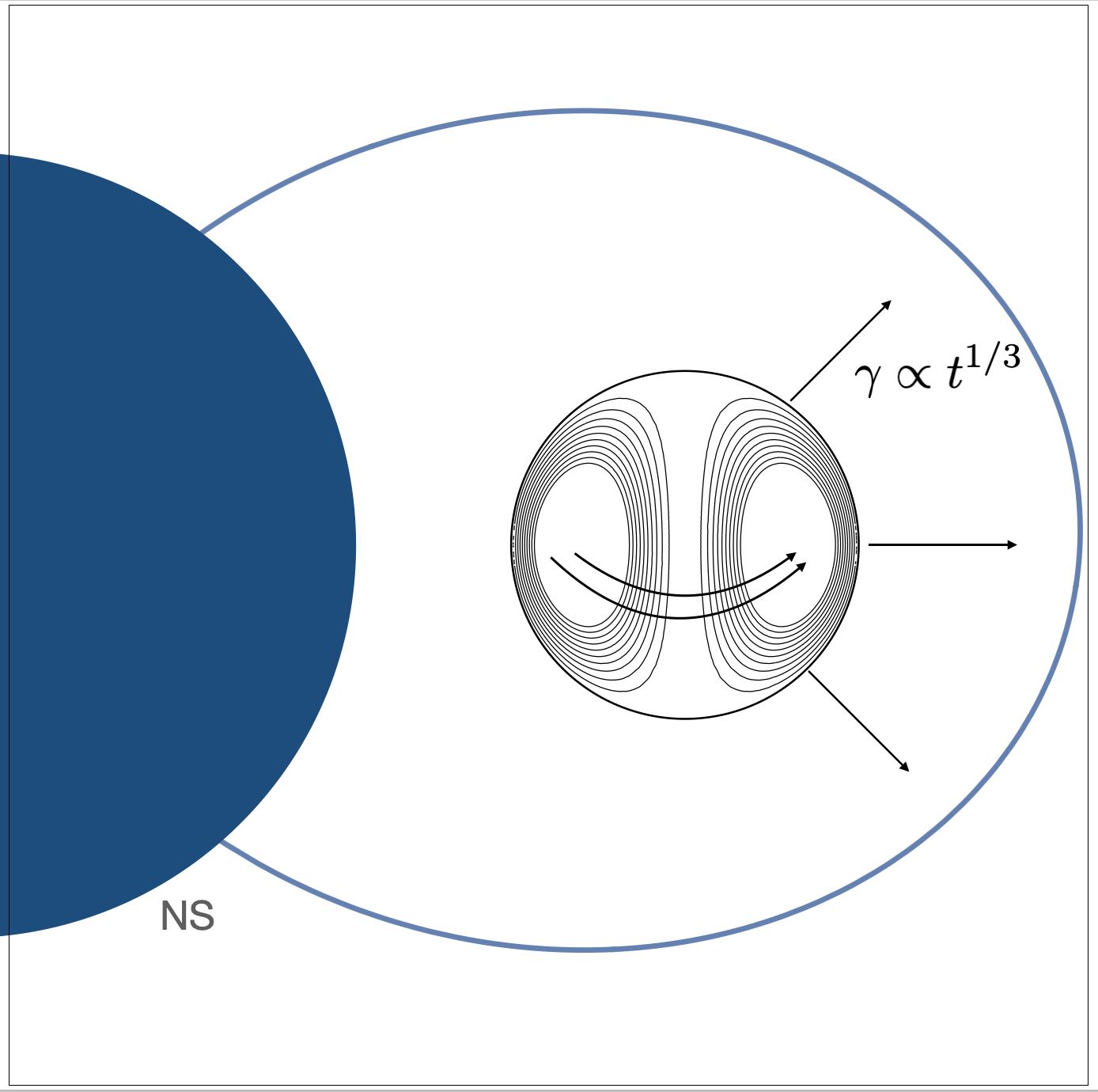
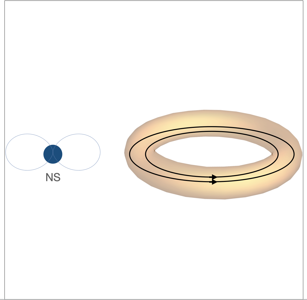
Figure 2: Cartoon of magnetic explosion of a spheromak. Left panel: a Solar flare-type even near the surface of the neutron star produces a magnetically disconnected magnetized cloud, a spheromak. Expansion is mostly equatorial. Right panel: During further expansion the magnetic flux in the tube remains constant. As a result the tube quickly reaches the force-balance with the wind. After that the flux tube forms a conically expanding structure.

3.5 Force-free pulse

Let us complement the above description with a related fully analytical non-linear model of temporarily spun-up neutron star, a jerk in a spin. The model discussed below is a variant of the magnetospheric ejection model, approximating a flare induced by crustal motion. The difference with the blob case is that now it is not assumed that an isolated magnetic bubble/flux tube is generated. Yet though the set-up is different, the conclusion is the same as above: magnetic perturbations do not generates shocks (but propagating EM pulses in this case).

Qualitatively, ”a jerk” in the angular rotation velocity $\Omega$ mimics a shearing motion of a patch of field lines (in fact, a star quake, often invoked as a driving mechanisms of flares, was shown to be a problematic model of flares by Levin & Lyutikov, 2012). The analytical model described below misses the magnetospheric dynamics, but it capture the wind dynamics.

If the magnetization of the wind is sufficiently high, we can actually build exact time-and-angle dependent model of propagation of the force-free electromagnetic pulse. As shown by Lyutikov (2011b) (see also Gralla & Jacobson, 2014) a stationary solution of monopolar magnetosphere by Michel (1973) can be generalized to arbitrary $\Omega=\Omega[r-t]g(\theta)$:

$$B_{r}=\left({R_{\rm LC}\over r}\right)^{2}B_{s}\mbox{}$$

$$\,B_{\phi}={R_{\rm LC}^{2}\sin\theta\over r}B_{s}\Omega(r-t)g(\theta)\mbox{}$$

$$\,E_{\theta}=B_{\phi}$$ (46)

see Fig 3- 4. This time-dependent nonlinear solution (nonlinear in a sense that the current is a non-linear function of the magnetic flux function) preserves both the radial and $\theta$ force balance. It can also be generalized to Schwarzschild metric using the Eddington-Finkelstein coordinates (Lyutikov, 2011b).

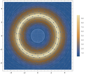
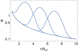
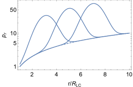
Figure 3: Left Panel: Structure of the magnetic field in the equatorial plane of an electromagnetic Gaussian pulse with amplitude $10$ times the average propagating through Michel’s wind. The peak of the pulse is at $r/R_{LC}=3$. The light cylinder  is at $\sqrt{x^{2}+y^{2}}=1$. Color scheme corresponds to $\ln B/B_{M}$, where $B_{M}$ is the local value of the magnetic field for Michel’s solution. Center Panel: plot of $B(r)$ showing EM pulse propagating with the wind for times $t=3,5,7$ (in units of $R_{LC}/c$); dashed line is the Michels’ solution. Right panel: plot of $p_{r}(r)$. The pulse propagates with the flow with constant relative amplitude, without experiencing any distortions.

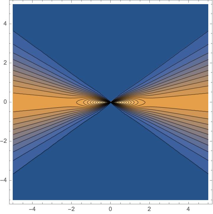
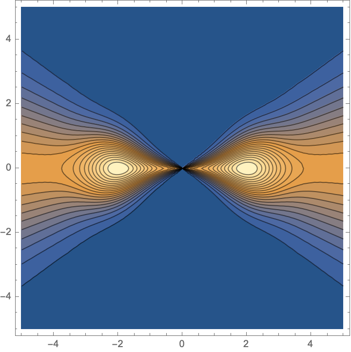
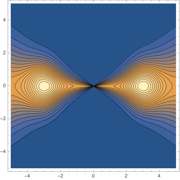
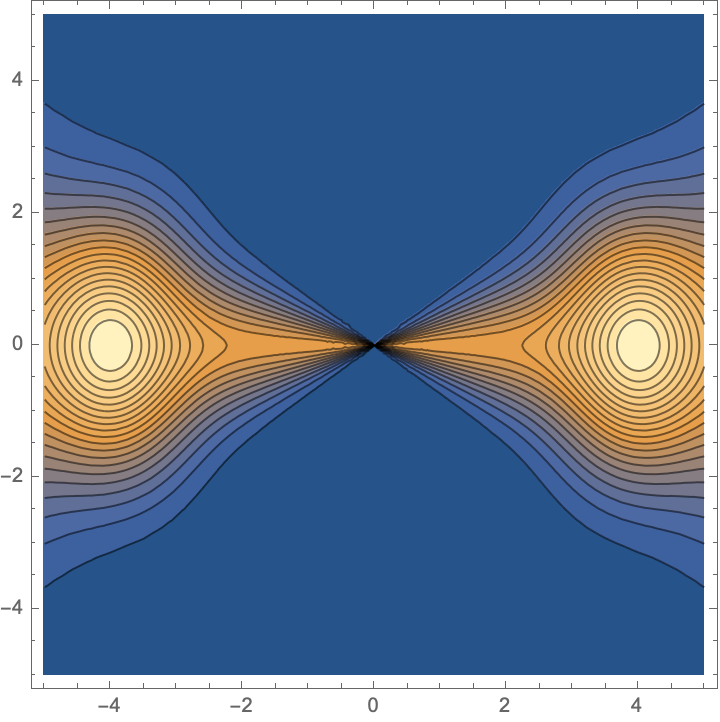
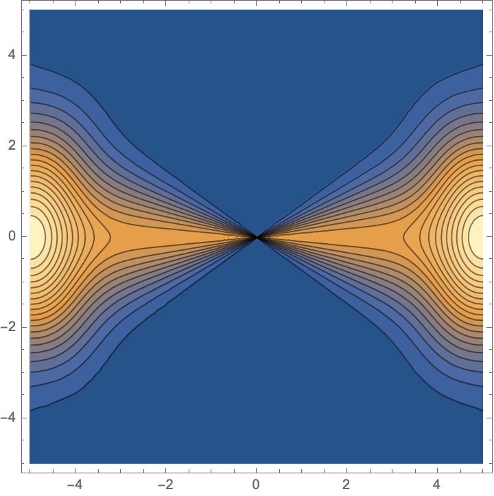
Figure 4: Dynamics of ejected flux tube with amplitude of $1$. Color plot is value of $B_{\phi}$. An ejection is parametrized as $g(\theta)=\sin^{10}\theta$, $\Omega=1+e^{(r-t)^{2}}$. Times are $t=0,1,...5$. These are fully analytical solutions, Eq. (46).

A pulse with $\Omega[r-t]g(\theta)$ propagates with radial 4-momentum

$$p_{r}=\frac{r^{2}\sin^{2}\theta(\Omega[r-t])^{2}g(\theta)^{2}}{\sqrt{1+r^{2}\sin^{2}\theta(\Omega[r-t])^{2}g(\theta)^{2}}}$$ (47)

which is larger than that of the wind for $\Omega[r-t]2g(\theta)\geq\Omega_{0}$, the constant value. Higher radial momentum of the ejected shell (than of the background flow) does not mean that plasma is swept-up: it’s just an EM pulse propagating through the accelerating wind.

The solutions (46) incorporate an EM pulse with a shape of arbitrary radial and angular dependence. For example, choosing a Gaussian pulse with $\Omega=(1+\delta e^{-(r-t)^{2}/(\Delta r)^{2}})\Omega_{0}$, solutions (46) represent a pulse with total power $\frac{1}{4}\sqrt{\pi}\delta\left(\sqrt{2}\delta+4\right)\approx\delta^{2}$ larger than the average wind power.

Since realistic dipolar magnetospheres do evolve asymptotically to the Michel (1973) solution (Bogovalov, 1999; Komissarov, 2006; Komissarov et al., 2009), we conclude that a force-free pulse with arbitrary amplitude and shape does not evolve (neither in $\theta$ nor $r-t$ coordinates) as the flow expands and accelerates.

This analytical example differs somewhat from the ejected blob/flux tube case in that it does not satisfy the “zero normal component of the magnetic field at the surface of the blob. Hence the importance of this example: magnetic ejection are either advected with the wind, or propagate as non-dissipative EM pulses. No shocks are generated.

The model of a ”jerk in spin” described above has a limitation that inside the magnetosphere the corresponding electromagnetic pulse, produced as presumed by the sudden crustal motion, is expected to break well before it reaches the light cylinder (Thompson & Duncan, 1996). As the crustal motion-generated EM pulse propagates through the magnetosphere, the relative amplitude of the O-mode scales as $\propto r^{3/2}$. This will lead to wave breaking (Akhiezer et al., 1975; Max et al., 1974; Drake et al., 1974) and dissipation of the wave energy (in simulations of Yuan et al., 2020, wave breaking was artificially prohibited by resetting the electric field to $E\leq B$ at every time step)

3.6 Applications to SGR 1935+2154 X-ray/radio flares

In the case of SGR 1935+2154, the unambiguously associated with a short pulse Burst-G by classification of Mereghetti et al. (2020), had peak X-ray luminosity of $\sim 10^{40}$ erg/s and total released energy $E_{f}\sim 10^{39}$ erg. The G burst was also particularly spectrally hard. The accompanying radio burst had $3\times 10^{34}$ ergs; the radio to high energy fluence was $F_{R}/F_{X}\sim 2\times 10^{-5}$. The period is $3.4$ seconds (so $R_{LC}=1.4\times 10^{10}$ cm, $R_{LC}/R_{NS}=1.4\times 10^{4}$). The spindown luminosity is $1.7\times 10^{34}$ erg s^-1, the surface magnetic field is $B_{NS}=2.2\times 10^{14}$ G (Israel et al., 2016)

Since the process of launching of any outflow is energetically the most demanding step, and assuming that a $\sim$ half of the energy was dissipated, we estimate the ejection energy as the energy of the X-ray burst. The required volume of the magnetosphere that got dissipated to power the X-ray flare is

$$R_{f}\sim\frac{E_{f}^{1/3}}{B_{NS}^{2/3}}=3\times 10^{3}\,{\rm cm}\mbox{}$$

$$\eta_{R}=\frac{R_{f}}{R_{NS}}=2\times 10^{-3}$$ (48)

A flare was just only 30 meters in size.

Expected wind coasting radius (7) is $R_{w}=1.7\times 10^{12}(\Gamma_{w}/100)$ cm, scale (12) is $R_{0}=1.7\times 10^{15}$ cm.

The flare released energy much larger than the magnetic energy at the light cylinder,

$$\frac{E_{f}}{E_{LC}}=6\times 10^{4}$$ (49)

The equipartition radius (40) evaluates to

$$\frac{R_{eq}}{R_{LC}}=2$$ (50)

Thus the expanding blob reached equipartition right near the light cylinder, consistent with our conclusion on the general FRB population.

Another problem for the wind models comes from fairly small compactness parameter. At peak luminosity of $\sim 10^{40}$ erg/s the compactness parameter $l_{c}$ evaluates to

$$l_{c}=\frac{\sigma_{T}L_{\gamma}}{m_{e}c^{4}\tau_{\gamma}}\leq 10^{3}$$ (51)

(actually smaller since the peak energy of the burst was $E_{p}\sim$ 65 keV$\ll m_{e}c^{2}$). Omitting for the sake of an argument the magnetic loading, the corresponding hydrodynamic terminal Lorentz factor is small

$$\Gamma_{f}\propto l_{c}^{1/6}\sim\mbox{few}$$ (52)

for duration of $\tau_{\gamma}\sim 10$ msec.

4 Discussion

We demonstrate that the wind models of FRBs are internally inconsistent on several grounds. The wind-type models of FBRs had a clear “good” point: if (only if !) one can make a relativistic shock in a relativistically receding wind, the combined Lorentz factor of the shock and (two times) the wind’s Lorentz factor make for an extremely high Lorentz factor shock, hence short durations from large distances.

There are serious problems with this scenario. First, regardless of the launching mechanism, the flare-generated outflow must be exceptionally clean, launching an outflow with the Lorentz factor at least few thousands, Eq. (9) assuming very low $\Gamma_{w}\sim 30$. This is about an order of magnitude higher than in GRBs. Wind models of the ejection are hopeless, the ejecta-wind must be millions of times cleaner than the preceding magnetar wind, Eq. (34). Impulsive ejections have an advantage that they can reach terminal Lorentz factors $\sim\mu_{0}$, compared with $\mu_{0}^{1/3}$ for steady state.

Most importantly, we argue that in contrast to the hydrodynamic explosions (when the terminal Lorentz factor is determined either by ion loading, or by pair freeze-out), the dynamics of the magnetic explosions is controlled by magnetic loading: the requirement of the conservation of the magnetic flux. Thus, in the case of magnetar explosions the dynamics is drastically different from the fluid case; instead of shocks with Lorentz factors close to a million, the explosions reach force-balance near the light cylinder and then either are advected with the wind as non-dissipative EM structure, or propagate as EM pulses.

Historically, the wind-type models of FBRs started, perhaps, with the Lyubarsky (2014) model. He advocated an EM pulse propagating in the wind (which is a correct model in our view), but the energetics of his model was $\geq 10^{50}$ ergs, in the ball park of GRBs, and clearly inconsistent with the FRB phenomenology. Finally we note that the original cyclotron instability model (Hoshino & Arons, 1991; Gallant et al., 1992; Hoshino et al., 1992) was developed to explain months long variations of Crab’s wisps, some ten orders of magnitude in time scale from the FRBs.

This work had been supported by NASA grants 80NSSC17K0757 and 80NSSC20K0910, NSF grants 1903332 and 1908590. I would like to thank Andrei Beloborodov, Yuri Lyubarsky and Lorenzo Sironi for discussions.

5 Data availability

The data underlying this article will be shared on reasonable request to the corresponding author.

References

- Akhiezer et al. (1975) Akhiezer, A. I., Akhiezer, I. A., Polovin, R. V., Sitenko, A. G., & Stepanov, K. N. 1975, Oxford Pergamon Press International Series on Natural Philosophy, 1
- Arons (1983) Arons, J. 1983, in AIP Conf. Ser., Vol. 101, Positron-Electron Pairs in Astrophysics, ed. M. L. Burns, A. K. Harding, & R. Ramaty, 163
- Arons & Scharlemann (1979) Arons, J., & Scharlemann, E. T. 1979, ApJ, 231, 854
- Babul & Sironi (2020) Babul, A.-N., & Sironi, L. 2020, MNRAS
- Barkov et al. (2021) Barkov, M. V., Luo, Y., & Lyutikov, M. 2021, ApJ, 907, 109
- Bellan (2000) Bellan, P. M. 2000, Spheromaks: a practical application of magnetohydrodynamic dynamos and plasma self-organization (Spheromaks: a practical application of magnetohydrodynamic dynamos and plasma self-organization/ Paul M. Bellan. London: Imperial College Press; River Edge, NJ: Distributed by World Scientific Pub. Co., c2000.)
- Beloborodov (2017) Beloborodov, A. M. 2017, ApJ, 843, L26
- Beloborodov (2020) —. 2020, ApJ, 896, 142
- Beloborodov & Thompson (2007) Beloborodov, A. M., & Thompson, C. 2007, ApJ, 657, 967
- Blandford & McKee (1976) Blandford, R. D., & McKee, C. F. 1976, Physics of Fluids, 19, 1130
- Bochenek et al. (2020) Bochenek, C. D., Ravi, V., Belov, K. V., Hallinan, G., Kocz, J., Kulkarni, S. R., & McKenna, D. L. 2020, Nature, 587, 59
- Bogovalov (1999) Bogovalov, S. V. 1999, A&A, 349, 1017
- Cameron et al. (2005) Cameron, P. B., Chandra, P., Ray, A., Kulkarni, S. R., Frail, D. A., Wieringa, M. H., Nakar, E., Phinney, E. S., Miyazaki, A., Tsuboi, M., Okumura, S., Kawai, N., Menten, K. M., & Bertoldi, F. 2005, Nature, 434, 1112
- CHIME/FRB Collaboration et al. (2020) CHIME/FRB Collaboration, Andersen, B. C., Bandura, K. M., Bhardwaj, M., Bij, A., Boyce, M. M., Boyle, P. J., Brar, C., Cassanelli, T., Chawla, P., Chen, T., Cliche, J. F., Cook, A., Cubranic, D., Curtin, A. P., Denman, N. T., Dobbs, M., Dong, F. Q., Fandino, M., Fonseca, E., Gaensler, B. M., Giri, U., Good, D. C., Halpern, M., Hill, A. S., Hinshaw, G. F., Höfer, C., Josephy, A., Kania, J. W., Kaspi, V. M., Landecker, T. L., Leung, C., Li, D. Z., Lin, H. H., Masui, K. W., McKinven, R., Mena-Parra, J., Merryfield, M., Meyers, B. W., Michilli, D., Milutinovic, N., Mirhosseini, A., Münchmeyer, M., Naidu, A., Newburgh, L. B., Ng, C., Patel, C., Pen, U. L., Pinsonneault-Marotte, T., Pleunis, Z., Quine, B. M., Rafiei-Ravandi, M., Rahman, M., Ransom, S. M., Renard, A., Sanghavi, P., Scholz, P., Shaw, J. R., Shin, K., Siegel, S. R., Singh, S., Smegal, R. J., Smith, K. M., Stairs, I. H., Tan, C. M., Tendulkar, S. P., Tretyakov, I., Vanderlinde, K., Wang, H., Wulf, D., & Zwaniga, A. V. 2020, Nature, 587, 54
- Coroniti (1990) Coroniti, F. V. 1990, ApJ, 349, 538
- Drake et al. (1974) Drake, J. F., Kaw, P. K., Lee, Y. C., Schmid, G., Liu, C. S., & Rosenbluth, M. N. 1974, Physics of Fluids, 17, 778
- Farrugia et al. (1995) Farrugia, C. J., Osherovich, V. A., & Burlaga, L. F. 1995, J. Geophys. Res., 100, 12293
- Gaensler et al. (2005) Gaensler, B. M., Kouveliotou, C., Gelfand, J. D., Taylor, G. B., Eichler, D., Wijers, R. A. M. J., Granot, J., Ramirez-Ruiz, E., Lyubarsky, Y. E., Hunstead, R. W., Campbell-Wilson, D., van der Horst, A. J., McLaughlin, M. A., Fender, R. P., Garrett, M. A., Newton-McGee, K. J., Palmer, D. M., Gehrels, N., & Woods, P. M. 2005, Nature, 434, 1104
- Gallant & Arons (1994) Gallant, Y. A., & Arons, J. 1994, ApJ, 435, 230
- Gallant et al. (1992) Gallant, Y. A., Hoshino, M., Langdon, A. B., Arons, J., & Max, C. E. 1992, ApJ, 391, 73
- Goldreich & Julian (1970) Goldreich, P., & Julian, W. H. 1970, ApJ, 160, 971
- Gralla & Jacobson (2014) Gralla, S. E., & Jacobson, T. 2014, MNRAS, 445, 2500
- Hibschman & Arons (2001) Hibschman, J. A., & Arons, J. 2001, ApJ, 560, 871
- Hoshino & Arons (1991) Hoshino, M., & Arons, J. 1991, Physics of Fluids B, 3, 818
- Hoshino et al. (1992) Hoshino, M., Arons, J., Gallant, Y. A., & Langdon, A. B. 1992, ApJ, 390, 454
- Hurley et al. (2005) Hurley, K., Boggs, S. E., Smith, D. M., Duncan, R. C., Lin, R., Zoglauer, A., Krucker, S., Hurford, G., Hudson, H., Wigger, C., Hajdas, W., Thompson, C., Mitrofanov, I., Sanin, A., Boynton, W., Fellows, C., von Kienlin, A., Lichti, G., Rau, A., & Cline, T. 2005, Nature, 434, 1098
- Israel et al. (2016) Israel, G. L., Esposito, P., Rea, N., Coti Zelati, F., Tiengo, A., Campana, S., Mereghetti, S., Rodriguez Castillo, G. A., Götz, D., Burgay, M., Possenti, A., Zane, S., Turolla, R., Perna, R., Cannizzaro, G., & Pons, J. 2016, MNRAS, 457, 3448
- Kennel & Coroniti (1984) Kennel, C. F., & Coroniti, F. V. 1984, ApJ, 283, 694
- Komissarov (2006) Komissarov, S. S. 2006, MNRAS, 367, 19
- Komissarov et al. (2009) Komissarov, S. S., Vlahakis, N., Königl, A., & Barkov, M. V. 2009, MNRAS, 394, 1182
- Levin & Lyutikov (2012) Levin, Y., & Lyutikov, M. 2012, MNRAS, 427, 1574
- Levinson (2010) Levinson, A. 2010, ApJ, 720, 1490
- Li et al. (2021) Li, C. K., Lin, L., Xiong, S. L., Ge, M. Y., Li, X. B., Li, T. P., Lu, F. J., Zhang, S. N., Tuo, Y. L., Nang, Y., Zhang, B., Xiao, S., Chen, Y., Song, L. M., Xu, Y. P., Liu, C. Z., Jia, S. M., Cao, X. L., Qu, J. L., Zhang, S., Gu, Y. D., Liao, J. Y., Zhao, X. F., Tan, Y., Nie, J. Y., Zhao, H. S., Zheng, S. J., Zheng, Y. G., Luo, Q., Cai, C., Li, B., Xue, W. C., Bu, Q. C., Chang, Z., Chen, G., Chen, L., Chen, T. X., Chen, Y. B., Chen, Y. P., Cui, W., Cui, W. W., Deng, J. K., Dong, Y. W., Du, Y. Y., Fu, M. X., Gao, G. H., Gao, H., Gao, M., Gu, Y. D., Guan, J., Guo, C. C., Han, D. W., Huang, Y., Huo, J., Jiang, L. H., Jiang, W. C., Jin, J., Jin, Y. J., Kong, L. D., Li, G., Li, M. S., Li, W., Li, X., Li, X. F., Li, Y. G., Li, Z. W., Liang, X. H., Liu, B. S., Liu, G. Q., Liu, H. W., Liu, X. J., Liu, Y. N., Lu, B., Lu, X. F., Luo, T., Ma, X., Meng, B., Ou, G., Sai, N., Shang, R. C., Song, X. Y., Sun, L., Tao, L., Wang, C., Wang, G. F., Wang, J., Wang, W. S., Wang, Y. S., Wen, X. Y., Wu, B. B., Wu, B. Y., Wu, M., Xiao, G. C., Xu, H., Yang, J. W., Yang, S., Yang, Y. J., Yang, Y.-J., Yi, Q. B., Yin, Q. Q., You, Y., Zhang, A. M., Zhang, C. M., Zhang, F., Zhang, H. M., Zhang, J., Zhang, T., Zhang, W., Zhang, W. C., Zhang, W. Z., Zhang, Y., Zhang, Y., Zhang, Y. F., Zhang, Y. J., Zhang, Z., Zhang, Z., Zhang, Z. L., Zhou, D. K., Zhou, J. F., Zhu, Y., Zhu, Y. X., & Zhuang, R. L. 2021, Nature Astronomy
- Lyubarsky (2014) Lyubarsky, Y. 2014, MNRAS, 442, L9
- Lyubarsky (2020) —. 2020, ApJ, 897, 1
- Lyubarsky (2021) —. 2021, Universe, 7, 56
- Lyubarsky & Kirk (2001) Lyubarsky, Y., & Kirk, J. G. 2001, ApJ, 547, 437
- Lyubarsky (2003) Lyubarsky, Y. E. 2003, MNRAS, 345, 153
- Lyutikov (2002a) Lyutikov, M. 2002a, Physics of Fluids, 14, 963
- Lyutikov (2002b) —. 2002b, ApJ, 580, L65
- Lyutikov (2006a) —. 2006a, MNRAS, 367, 1594
- Lyutikov (2006b) Lyutikov, M. 2006b, in APS April Meeting Abstracts, APS Meeting Abstracts, X3.003
- Lyutikov (2006c) —. 2006c, New Journal of Physics, 8, 119
- Lyutikov (2010) —. 2010, Phys. Rev. E, 82, 056305
- Lyutikov (2011a) —. 2011a, MNRAS, 411, 422
- Lyutikov (2011b) —. 2011b, Phys. Rev. D, 83, 124035
- Lyutikov (2017) Lyutikov, M. 2017, Physics of Fluids, 29, 047101
- Lyutikov (2021) Lyutikov, M. 2021, arXiv e-prints, arXiv:2102.07010
- Lyutikov & Blandford (2003) Lyutikov, M., & Blandford, R. 2003, arXiv e-prints, astro
- Lyutikov & Camilo Jaramillo (2017) Lyutikov, M., & Camilo Jaramillo, J. 2017, ApJ, 835, 206
- Lyutikov & Gourgouliatos (2011) Lyutikov, M., & Gourgouliatos, K. N. 2011, Sol. Phys., 270, 537
- Lyutikov & Hadden (2012) Lyutikov, M., & Hadden, S. 2012, Phys. Rev. E, 85, 026401
- Lyutikov et al. (2016) Lyutikov, M., Komissarov, S. S., & Porth, O. 2016, MNRAS, 456, 286
- Lyutikov & Popov (2020) Lyutikov, M., & Popov, S. 2020, arXiv e-prints, arXiv:2005.05093
- Lyutikov & Rafat (2019) Lyutikov, M., & Rafat, M. 2019, arXiv e-prints, arXiv:1901.03260
- Max et al. (1974) Max, C. E., Arons, J., & Langdon, A. B. 1974, Phys. Rev. Lett., 33, 209
- Mehta et al. (2021) Mehta, R., Barkov, M., & Lyutikov, M. 2021, MNRAS, 506, 6093
- Mereghetti et al. (2020) Mereghetti, S., Savchenko, V., Ferrigno, C., Götz, D., Rigoselli, M., Tiengo, A., Bazzano, A., Bozzo, E., Coleiro, A., Courvoisier, T. J. L., Doyle, M., Goldwurm, A., Hanlon, L., Jourdain, E., von Kienlin, A., Lutovinov, A., Martin-Carrillo, A., Molkov, S., Natalucci, L., Onori, F., Panessa, F., Rodi, J., Rodriguez, J., Sánchez-Fernández, C., Sunyaev, R., & Ubertini, P. 2020, ApJ, 898, L29
- Metzger et al. (2017) Metzger, B. D., Berger, E., & Margalit, B. 2017, ApJ, 841, 14
- Metzger et al. (2019) Metzger, B. D., Margalit, B., & Sironi, L. 2019, MNRAS, 485, 4091
- Michel (1969) Michel, F. C. 1969, ApJ, 158, 727
- Michel (1973) —. 1973, ApJ, 180, L133
- Paczynski (1986) Paczynski, B. 1986, ApJ, 308, L43
- Palmer et al. (2005) Palmer, D. M., Barthelmy, S., Gehrels, N., Kippen, R. M., Cayton, T., Kouveliotou, C., Eichler, D., Wijers, R. A. M. J., Woods, P. M., Granot, J., Lyubarsky, Y. E., Ramirez-Ruiz, E., Barbier, L., Chester, M., Cummings, J., Fenimore, E. E., Finger, M. H., Gaensler, B. M., Hullinger, D., Krimm, H., Markwardt, C. B., Nousek, J. A., Parsons, A., Patel, S., Sakamoto, T., Sato, G., Suzuki, M., & Tueller, J. 2005, Nature, 434, 1107
- Piran (2004) Piran, T. 2004, Reviews of Modern Physics, 76, 1143
- Plotnikov & Sironi (2019) Plotnikov, I., & Sironi, L. 2019, MNRAS, 485, 3816
- Porth et al. (2017) Porth, O., Buehler, R., Olmi, B., Komissarov, S., Lamberts, A., Amato, E., Yuan, Y., & Rudy, A. 2017, Space Sci. Rev., 207, 137
- Porth et al. (2014) Porth, O., Komissarov, S. S., & Keppens, R. 2014, MNRAS, 438, 278
- Rees & Gunn (1974) Rees, M. J., & Gunn, J. E. 1974, MNRAS, 167, 1
- Ridnaia et al. (2020) Ridnaia, A., Svinkin, D., Frederiks, D., Bykov, A., Popov, S., Aptekar, R., Golenetskii, S., Lysenko, A., Tsvetkova, A., Ulanov, M., & Cline, T. 2020, arXiv e-prints, arXiv:2005.11178
- Sironi & Spitkovsky (2009) Sironi, L., & Spitkovsky, A. 2009, ApJ, 698, 1523
- Sironi & Spitkovsky (2011) —. 2011, ApJ, 741, 39
- Thompson & Duncan (1996) Thompson, C., & Duncan, R. C. 1996, ApJ, 473, 322
- Yuan et al. (2020) Yuan, Y., Beloborodov, A. M., Chen, A. Y., & Levin, Y. 2020, ApJ, 900, L21