Modeling high-speed gas–particle flows relevant to spacecraft landings: A review and perspectives

Abstract

The interactions between rocket exhaust plumes and the surface of extraterrestrial bodies during spacecraft landings involve complex multiphase flow dynamics that pose significant risk to space exploration missions. The two-phase flow is characterized by high Reynolds and Mach number conditions with particle concentrations ranging from dilute to close-packing. Low atmospheric pressure and gravity typically encountered in landing environments combined with reduced optical access by the granular material pose significant challenges for experimental investigations. Consequently, numerical modeling is expected to play an increasingly important role for future missions. This article presents a review and perspectives on modeling high-speed disperse two-phase flows relevant to plume-surface interactions (PSI). We present an overview of existing drag laws, with origins from 18th-century cannon fire experiments and new insights from particle-resolved numerical simulations. While the focus here is on multiphase flows relevant to PSI, much of the same physics are shared by other compressible gas–particle flows, such as coal-dust explosions, volcanic eruptions, and detonation of solid material.

1 Introduction

During the powered landing of a spacecraft on lunar and planetary bodies, impinging exhaust gases generate a strong recirculation region that fluidize the surface and eject loose granular matter (see Fig. 1). Plume-surface interactions (PSI) are capable of destabilizing the lander and dislodging dust and debris at high speeds that can damage exposed hardware, reduce visibility, and spoof landing sensors. Mitigating the risks of PSI requires a detailed understanding of the multiphase dynamics under such extreme conditions. While the last several decades have seen significant advancements in simulation and modeling techniques for incompressible particle-laden flows (Crowe et al., 1996; Balachandar and Eaton, 2010; Fox, 2012; Tenneti and Subramaniam, 2014), much less attention has been paid to high-speed (compressible) two-phase flows. This article presents a review and perspectives on this topic.

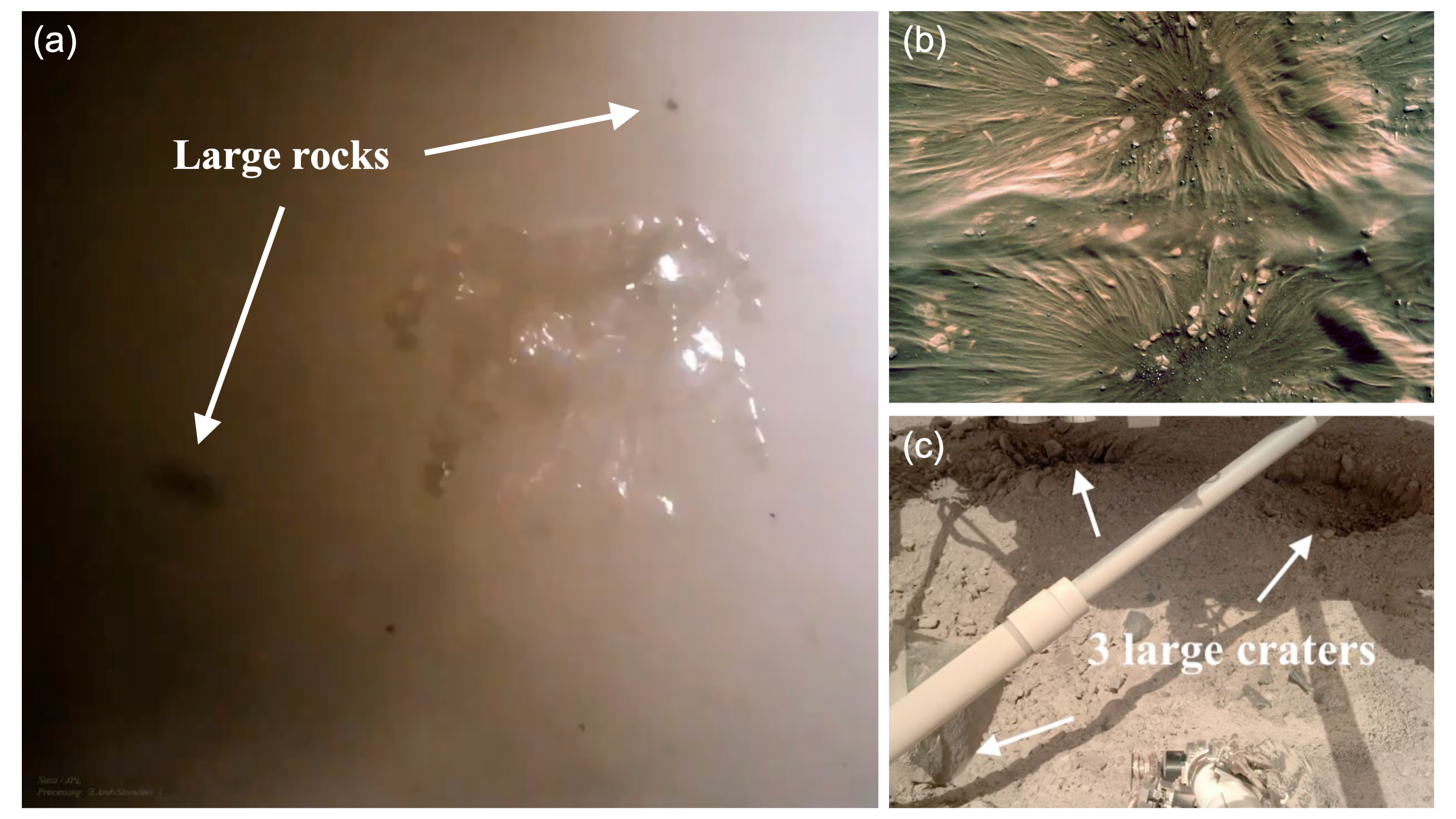
Figure 1: Plume-surface interactions during spacecraft propulsive landings represent a key challenge for space exploration. (a-b) Final descent of NASA’s Perseverance rover on February 18, 2021 showing (a) ejected dust and rocks and (b) erosion of martian regolith during the Sky Crane maneuver. (c) Craters formed by rocket plumes beneath NASA’s InSight lander. Images adapted from NASA/JPL-Caltech.

In this section, examples of PSI from past landing events and the associated flow physics are presented. The remainder of the article focuses on the fundamental dynamics and processes of compressible gas–particle flows. Origins of existing models and new insights gleaned from particle-resolved simulations are reported. Particular attention is paid to interphase coupling under dilute and moderately dense concentrations at finite Mach number. We summarize classical drag laws in addition to models for unsteady contributions due to added mass and ‘pseudo’ turbulence during shock-particle interactions.

1.1 Impact of PSI from previous landings

The detrimental effects of PSI from previous lunar and martian missions are well documented (Christensen et al., 1967; Foreman, 1967; O’Brien et al., 1970; Clark, 1970; Jaffe, 1971; Taylor, 1972; Hutton et al., 1980; O’Brien, 2009; Gómez-Elvira et al., 2014). In fact, four of the six Apollo landings suffered from hindered visibility caused by ejected granular material during landing. Suspension of lunar dust was found to deposit on equipment located 17 m from Apollo 11 and 160 m from Apollo 12 (O’Brien, 2009). Hardware on the Surveyor III craft experienced pitting and cracking as a result of sandblasting from high-speed ejecta during the Apollo 12 landing (Jaffe, 1971; Immer et al., 2011b, a). Particles were estimated to have traveled at speeds in excess of 100 m/s. During the Apollo 15 landing, the lunar module experienced a 12-degree tilt at touchdown, almost terminating the mission (McDivitt, 1971). Due to the lack of an atmosphere on the Moon, smaller particles suspended during the Apollo landings are estimated to have reached escape velocity, posing hazards to orbital hardware (Lane et al., 2008).

In an effort to mitigate the negative effects of PSI, NASA’s 2012 Mars Science Laboratory (MSL) mission introduced the Sky Crane maneuver for the final descent of the Curiosity lander. The rover was lowered down on a bridle from an altitude of 7.5 m to prevent close contact between the rocket engines and the planet’s surface. Compared to the Moon, the thin (but finite) martian atmosphere inhibits the spreading of exhaust gas, resulting in collimated rocket plumes that generate highly localized impingement pressures (Mehta et al., 2013) and the formation of craters (see Fig. 1(c)). A significant amount of soil and debris was lifted during MSL, which is believed to have damaged one of the Curiosity rover’s two wind sensors (Gómez-Elvira et al., 2014). The same Sky Crane maneuver was also used for the Mars 2020 mission. As shown in Fig. 1, erosion of martian soil was observed during descent of the Perseverance rover, resulting in the liberation and ejection of large rocks. Meanwhile, planned sample return missions and anticipated crewed missions with higher payloads precludes the use of Sky Crane.

1.2 Multiphase flow dynamics during PSI

Incorporating the effects of PSI into the design stage of next-generation landers is a necessary step to minimize risk and ensure the success of future missions. What makes this so challenging are the wide range of flow regimes that coexist (see Fig. 2). The exhaust gas leaving the rocket nozzle is supersonic and chemically reacting, giving rise to a Mach disk followed by expansion waves and a plate (standoff) shock just above the surface. The Reynolds number at the exit of the nozzle is typically $\mbox{\rm Re}=\mathcal{O}(10^{5})$ and the Knudsen number of the exhaust gas is sufficiently low (Mehta et al., 2013), thus the flow is continuum and highly turbulent when the lander is within a few meters of the surface.

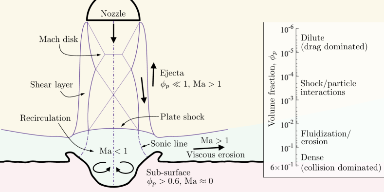
Figure 2: Schematic of the fluid-particle dynamics present during a landing event highlighting regions of varying Mach number, Ma, and volume fraction, $\phi_{p}$.

The particle volume fraction, $\phi_{p}$, generally decreases with elevation, from near close packing ($\phi_{p}>0.6$) at the surface to highly dilute above the plate shock. Within the recirculation region (sometimes referred to as the stagnation bubble (Mehta et al., 2013)), high-pressure subsonic flow fluidizes the soil. The impinging gas forms shock waves parallel to the surface and deflects the plume radially outward. The deflected plume accelerates to supersonic speeds, inducing high shear stress on the surface that lifts the soil into the boundary layer–so-called viscous erosion (Metzger et al., 2009). Ejected particles interact with turbulence in the shear layer and shock waves throughout the exhaust plume where the concentration is low ($\phi_{p}\ll 1$) and the gas-phase Mach number, Ma, is high. Interphase coupling between particles and turbulence in high-speed shear layers are capable of altering pressure fluctuations radiating outwards from the plume (Krothapalli et al., 2003; Buchta et al., 2019) and generating flow instabilities analogous to two-fluid flows (McFarland et al., 2016).

The physical mechanisms contributing to erosion vary depending on the rocket thrust, atmospheric conditions of the landing environment, and physical soil properties. Table 1 lists atmospheric conditions at the surface of Earth, the Moon, and Mars. Regolith (the upper layer of soil) on the Moon is tightly packed due to its near-vacuum conditions, preventing the exhaust gas from penetrating deep within. Thus, erosion is primarily a consequence of shear induced by the viscous flow above the surface (Hutton, 1968; Metzger et al., 2009), causing particles to spread far from the lander. Due to the lack of an atmosphere, the Moon is continually bombarded with small meteorites and its regolith exhibits a wide size distribution. In contrast, regolith on Mars is exposed to atmospheric wind and tends to be more spherical (Sullivan et al., 2005). The stagnation pressure exerted by the jet exceeds the bearing capacity of martian soil and compresses/evacuates the upper layer to form a deep crater (Metzger et al., 2009), which redirects the two-phase flow up towards the lander.

Table 1: Typical atmospheric conditions at the surface of Earth, the Moon, and Mars.

	Earth	Moon	Mars
Gravitational acceleration [$\rm{m/s^{2}}$]	$9.81$	$1.62$	$3.72$
Pressure [$\rm{mbar}$]	$1013.25$	$3\times 10^{-12}$	$5$–$10$
Density [$\rm{kg/m^{3}}$]	$1.2$	$\approx 0$	$1.66\times 10^{-2}$
Dynamic viscosity [$\rm{Ns/m^{2}}$]	$1.8\times 10^{-5}$	N/A	$1.5\times 10^{-5}$
Sound speed [$\rm{m/s}$]	$343$	N/A	$264$

1.3 Modeling PSI

Theoretical and experimental studies of PSI date back to the early 1960s (Spady, 1962; Roberts, 1963; Land and Clark, 1965; Roberts, 1966; Hutton, 1969). Roberts (1963) developed the first model to describe the erosion and subsequent transport of dust beneath a rocket for lunar environments. The erosion rate was determined from a balance between shear stress exerted by the plume and the threshold shear strength of the soil. However, the model neglected aerodynamic forces on the particles, and comparisons to laboratory-scale experiments showed only marginal agreement (Hutton, 1968). Metzger et al. (2008) modified Roberts’ theory by incorporating the particle size distribution of lunar soil and imposing ejection angles inferred from Apollo landing videos. However, the authors conclude that a better understanding of the aerodynamic forces and erosion process in supersonic flow regimes are needed. In addition, recent laboratory experiments have revealed that the threshold friction velocity to initiate saltation (and ensuing erosion) differs substantially in low pressure environments like Mars, yet existing scaling laws are unable to capture this (Sullivan and Kok, 2017; Andreotti et al., 2021).

Particle motion during PSI is a consequence of fluid-particle and particle-particle interactions at the microscale, i.e., fluid stresses and contact dynamics at the sub-particle level. Fluid forces acting on each particle depend non-linearly on the local Reynolds number, Mach number, and volume fraction. Inter-particle forces arising from collisions and sliding/rolling friction vary based on the physical properties of the regolith. In recent years, Eulerian-based two-fluid models (Gale et al., 2017; Balakrishnan and Bellan, 2018; Gale et al., 2020; Balakrishnan and Bellan, 2019; Chinnappan et al., 2021; Balakrishnan and Bellan, 2021) and particle-based methods (He et al., 2012; Morris et al., 2015; Rahimi et al., 2020; Shallcross, 2021) of PSI have been conducted that explicitly account for these interactions. Yet, the underlying models these simulations are built upon (e.g., drag, sub-grid scale turbulence, etc.) were largely developed for incompressible flows. While the aerodynamics of high-speed projectiles have been studied for centuries (namely in the context of ballistics), there has been significant developments in recent years, largely owing to the advent of high-performance computing. This article focuses specifically on gas–particle interactions: the origins of existing models; progress in theoretical understanding over recent years; and perspectives for future model development.

2 Scale separation

The range of scales of motion in particle-laden flows are vast (see Fig. 3 for the simple case of an isolated particle). When the flow is incompressible, the smallest scales are typically on the order of the particle diameter, $d_{p}$. In turbulent flows, the smallest eddy size (the Kolmogorov, or dissipation length scale) is also important. Relevant time scales include the particle response time, $\tau_{p}=\rho_{p}d_{p}^{2}/(18\mu_{f})$, where $\rho_{p}$ is the particle density and $\mu_{f}$ is the fluid viscosity, in addition to time scales associated with the fastest turbulent velocity fluctuations. When gas-phase compressibility is important, information travels near or exceeds the sound speed, $c$. An acoustic time scale can be defined using $c$ and a relevant length scale, e.g., $d_{p}/c$, which is often much smaller than $\tau_{p}$. For example, a solid particle with density $\rho_{p}=3000$ kg/m³ and diameter $d_{p}=100$ $\upmu$m in air results in $\tau_{p}\approx 0.1$ s and $d_{p}/c\approx 0.3$ $\upmu$s! The interaction between shock waves and suspensions of particles involves length scales spanning the shock thickness (order of the mean free path of gas molecules), to wakes past particles at scales larger than the particle diameter. In the context of PSI, the largest scales of interest may include the full landing site, which can span kilometers.

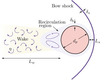
Figure 3: Schematic of a supersonic flow past a spherical particle (particle moving from left to right). Various length scales that are present (in approximately increasing magnitude): shock wave thickness $\delta_{s}$; boundary layer thickness $\delta_{b}$; Kolmogorov length scale $\eta$; shock standoff distance $L_{s}$; particle diameter $d_{p}$; and wake length $L_{w}$.

A key challenge in modeling any multiphase flow system is properly capturing the length- and time-scales at play. The equation of motion for a particle with mass $m_{p}$ and velocity $\mbox{\boldmath{$v$}}_{p}$ traveling through a viscous fluid can be expressed as

$$m_{p}\frac{{\rm d}\mbox{\boldmath{$v$}}_{p}}{{\rm d}t}=\int_{S}\left(\check{\mbox{\boldmath{$\sigma$}}}_{f}-\check{p}_{f}\mathbb{I}\right)\boldsymbol{\mbox{\boldmath{$\cdot$}}}\mbox{\boldmath{$n$}}\,{\rm d}S+\mbox{\boldmath{$F$}}_{\rm ext},$$ (1)

where $\check{p}_{f}$ is the fluid pressure, $\check{\mbox{\boldmath{$\sigma$}}}_{f}$ is the viscous stress tensor, $n$ is the unit normal vector outward from the particle surface $S$, $\mathbb{I}$ is the identity tensor, and $\mbox{\boldmath{$F$}}_{\rm ext}$ are external body forces. Here, the $\check{(\cdot)}$ notation denotes a microscale quantity prior to any averaging. It becomes immediately apparent that a numerical solution to Eq. (1) requires sub-particle scale resolution. Particle-resolved simulations for incompressible flows usually employ grid spacing 20–40 times smaller than the particle diameter (Tenneti and Subramaniam, 2014)–even finer resolution is typically required for compressible flows–which becomes extremely computationally demanding when the system size of interest is much larger than the size of an individual particle. Thus, direct solutions to the conservation equations are rarely practical. Below we introduce the averaged equations of motion and the challenges that arise.

2.1 Averaged equations

Obtaining a mathematical description that captures the multi-scale nature of two-phase flows typically involves ensemble averaging (Zhang and Prosperetti, 1997) or volume filtering (Anderson and Jackson, 1967; Capecelatro and Desjardins, 2013). The main idea is to apply an averaging volume (or filter) with a characteristic size comparable to the inter-particle spacing to replace surface fluxes with volumetric source terms. This is analogous to large-eddy simulation (LES) of single-phase flows, and similarly results in unclosed terms that require models. Unlike in single-phase LES, the averaging procedure omits the volume occupied by particles, and consequently differentiation and filtering do not commute. This produces sub-filtered (or subgrid-scale) contributions at the surface of each particle.

Applying such an averaging operation to the viscous compressible Navier–Stokes equations–recall the flow within the exhaust plume during PSI can be treated as continuum–yields equations for mass, momentum, and energy (Shallcross et al., 2020)

$$\frac{\partial\phi_{f}\rho_{f}}{\partial t}+\nabla\boldsymbol{\mbox{\boldmath{$\cdot$}}}\left(\phi_{f}\rho_{f}\mbox{\boldmath{$u$}}_{f}\right)=0,$$ (2)

$$\frac{\partial\phi_{f}\rho_{f}\mbox{\boldmath{$u$}}_{f}}{\partial t}+\nabla\boldsymbol{\mbox{\boldmath{$\cdot$}}}(\phi_{f}\left\{\rho\mbox{\boldmath{$u$}}_{f}\mbox{\boldmath{$u$}}_{f}+\mbox{\boldmath{$R$}}_{f}\right\})=\phi_{f}\nabla\boldsymbol{\mbox{\boldmath{$\cdot$}}}\left(\mbox{\boldmath{$\sigma$}}_{f}-p_{f}\mathbb{I}\right)+\mbox{\boldmath{$F$}}_{p},$$ (3)

and

$$\frac{\partial\phi_{f}\rho_{f}E_{f}}{\partial t} +\nabla\boldsymbol{\mbox{\boldmath{$\cdot$}}}\left(\phi_{f}\rho_{f}E_{f}\mbox{\boldmath{$u$}}_{f}\right)+\nabla\boldsymbol{\mbox{\boldmath{$\cdot$}}}(\phi_{f}(p_{f}\mbox{\boldmath{$u$}}_{f}-\mbox{\boldmath{$u$}}_{f}\boldsymbol{\mbox{\boldmath{$\cdot$}}}\mbox{\boldmath{$\sigma$}}_{f}))+\phi_{f}\nabla\boldsymbol{\mbox{\boldmath{$\cdot$}}}\mbox{\boldmath{$q$}}_{f}$$ (4)

$$=-p_{f}\frac{\partial\phi_{f}}{\partial t}+\mbox{\boldmath{$\sigma$}}_{f}\boldsymbol{\mbox{\boldmath{$:$}}}\nabla\left(\phi_{p}\mbox{\boldmath{$u$}}_{p}\right)+\mbox{\boldmath{$u$}}_{p}\boldsymbol{\mbox{\boldmath{$\cdot$}}}\mbox{\boldmath{$F$}}_{p}+Q_{p}-\nabla\boldsymbol{\mbox{\boldmath{$\cdot$}}}\left(\phi_{f}\{\mbox{\boldmath{$R$}}_{p}+\frac{1}{2}\mbox{\boldmath{$R$}}_{u}-\mbox{\boldmath{$R$}}_{\sigma}\}\right),$$

where $\phi_{f}=1-\phi_{p}$ is the fluid-phase volume fraction, $\rho_{f}$ is the fluid density, $\mbox{\boldmath{$u$}}_{f}$ the fluid velocity, $\mbox{\boldmath{$u$}}_{p}$ is the particle-phase velocity (in an Eulerian frame of reference), and $E_{f}$ the total energy. Interphase coupling takes place through momentum exchange, $\mbox{\boldmath{$F$}}_{p}$, that requires models for drag and other forces acting on the particle (see Sec. 3), and heat exchange, $Q_{p}$, typically modeled using Nusselt-number correlations. The first term on the right-hand side of Eq. (4) can be thought of as a $pDV$ work term due to particles entering and leaving a control volume (Lhuillier et al., 2010). By employing the particle-phase continuity equation and assuming constant particle density, this can be replaced with $-p_{f}\nabla\boldsymbol{\mbox{\boldmath{$\cdot$}}}\left(\phi_{p}\mbox{\boldmath{$u$}}_{p}\right)$ (Houim and Oran, 2016), which may be more convenient in a numerical implementation.

In Eq. (3), $\mbox{\boldmath{$R$}}_{f}$ is a residual stress that arises from filtering the non-linear convective term. Because the fluid velocity fluctuations may originate at the particle scale, the physics that govern this unclosed term differs significantly from the Reynolds stress appearing in classical single-phase flows. In fact, this term may be non-zero even in laminar flows (e.g., via steady wakes), and is therefore termed a pseudo turbulent Reynolds stress (Mehrabadi et al., 2015). While it is typically neglected in incompressible flow models, recent work has shown that $\mbox{\boldmath{$R$}}_{f}$ can contribute to a significant portion of the total kinetic energy during shock-particle interactions (Hosseinzadeh-Nik et al., 2018; Sen et al., 2018; Mehta et al., 2019a; Osnes et al., 2019; Shallcross et al., 2020). Special care needs to be taken when distinguishing the sub-filter scale velocity fluctuations originating from large-scale turbulent motion (via a classical energy cascade) and those induced by particles (pseudo turbulence). This will be revisited in Sec. 4.

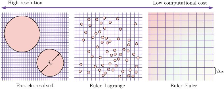
Figure 4: Different modeling approached for simulating gas–particle flows. Left: Particle-resolved simulations directly solve the gas-phase equations with grid spacing $\Delta x\ll d_{p}$. Interphase coupling takes place through boundary conditions at the surface of each particle. At this scale, drag is an output. Middle: Euler–Lagrange (EL) methods track individual particles and solve the fluid on a grid with $\Delta x\approx d_{p}$ (highly-resolved EL) or $\Delta x\gg d_{p}$ (course EL). Requires closure models for drag and sub-grid scale turbulence. Right: Euler–Euler (EE) methods solve both phases on the grid and require closure models for gas-particle and particle-particle interactions.

Additional unclosed terms appear in Eq. (4) that account for work due to the subgrid-scale pressure and viscous stress ($\mbox{\boldmath{$R$}}_{p}$ and $\mbox{\boldmath{$R$}}_{\sigma}$) and a triple product of subgrid-scale velocity fluctuations, $\mbox{\boldmath{$R$}}_{u}$. Particle-resolved direct numerical simulations (PR–DNS) of shock waves traveling through arrays of randomly distributed particles have demonstrated that $\mbox{\boldmath{$R$}}_{p}$ and $\mbox{\boldmath{$R$}}_{\sigma}$ are relatively small compared to the other terms in Eq. (4) (Mehta et al., 2019a; Shallcross et al., 2020), and Shallcross et al. (2020) showed that $\mbox{\boldmath{$R$}}_{u}\approx 2\mbox{\boldmath{$u$}}_{f}\cdot\mbox{\boldmath{$R$}}_{f}$. Thus, accurate solutions of the averaged compressible Navier–Stokes equations namely require validated models for the pseudo-turbulent Reynolds stress, $\mbox{\boldmath{$R$}}_{f}$, and momentum exchange, $\mbox{\boldmath{$F$}}_{p}$. Closure models have been proposed for these terms, but for most part are only valid in the incompressible or dilute limit. This is the focus of Secs. 3 and 4.

The same averaging procedure could be extended to the particle phase as well, resulting in the so-called Euler–Euler (EE) or two-fluid method. This gives rise to even more unclosed terms that require constitutive relations for the solid-phase rheology. While this is outside the scope of the present article, the full set of compressible EE equations can be found in Houim and Oran (2016); Balakrishnan and Bellan (2018); Fox (2019). Alternatively, Euler–Lagrange (EL) methods (also referred to as CFD–DEM in the chemical engineering literature) track individual particles and couple them to the averaged fluid equations. Figure 4 shows an illustration of these different modeling approaches.

2.2 Ill-posedness and hyperbolicity

In addition to producing a number of terms that require closure, it is also well established that two-phase models with rigid particles can become ill-posed due to lack of hyperbolicity (Lhuillier et al., 2013). In general, the compressible EE equations have imaginary characteristics that can lead to unphysical instabilities. This has been shown to give rise to spurious volume fraction disturbances during shock-particle interactions (Theofanous et al., 2018). EL methods generally remain hyperbolic due to the Lagrangian treatment of the particle phase, though they could be susceptible to similar numerical instabilities if inter-particle contact is not treated explicitly (Theofanous and Chang, 2017). Numerous attempts have been made to restore hyperbolicity starting with Stuhmiller (1977), and seems only very recently to be properly resolved (Fox et al., 2020).

Hyperbolicity depends strongly on the nature of the closure models. It is well established that the pressure gradient force acting on the particles (termed the Archimedes force) is the source of ill-posedness. Until recently, many authors have resorted to neglecting the Archimedes force or adding an ad-hoc ‘turbulent dispersion’ force to stabilize the solution, which compromises the physical accuracy (Lhuillier et al., 2013). Because the Archimedes force is proportional to the density ratio, these issues are more prevalent in bubbly as compared to gas–particle flows. Balakrishnan and Bellan (2021) analyzed the hyperbolicity of a compressible two-fluid model for simulations of supersonic jet-induced cratering on a granular bed. It was found that the system is hyperbolic in most regions except in the vicinity of the crater, particularly where the particle compaction is high ($\phi_{p}>0.6$). They conclude that high compaction alone is not a sufficient criterion for the system of equations to become degenerate.

An alternative approach to the ad-hoc corrections listed above is to take into account the velocity fluctuations of both phases, which necessitates additional closure for $\mbox{\boldmath{$R$}}_{f}$  (Lhuillier et al., 2013). Fox (2019) showed that starting from a well-defined microscale description, it is possible to derive a hyperbolic two-fluid model wherein the fluxes and source terms have unambiguous definitions. Starting from the Boltzmann–Enskog kinetic equations for a binary system, a two-fluid model for fully compressible fluid–particle flows was derived without exclusion of the Archimdes force. A rigorous analysis of this model showed that it is hyperbolic for gas–particle flows with $\rho_{p}/\rho_{f}\gg 1$. The following year, Fox et al. (2020) extended the model to arbitrary density ratios by including the added mass of the fluid on the particle in addition to fluid-mediated interactions between particles. An additional equation to include $\mbox{\boldmath{$R$}}_{f}$ in the fluid phase was also proposed. It was shown that pseudo turbulence has no effect on hyperbolicity but it is needed to ensure conservation. Details on the added mass treatment are given in Sec. 3.3 and models for $\mbox{\boldmath{$R$}}_{f}$ are given in Sec. 4.

3 Forces acting on a particle

As shown in Fig. 2 and discussed in Sec. 1, PSI spans dilute to dense particle-laden flow regimes. In this section, we first review the state-of-the-art in modeling the forces acting on an isolated particle, then move on to extensions to multi-particle systems. In the case of an isolated particle moving through an incompressible fluid at low Reynolds numbers (Stokes flow), Basset (1888), Boussinesq (1885), and Oseen (1927) decomposed the hydrodynamic force (the first term on the right-hand side of Eq. (1)) into separate contributions: the quasi-steady drag force $\mbox{\boldmath{$F$}}_{qs}$; undisturbed flow forces $\mbox{\boldmath{$F$}}_{un}$ (sometimes denoted as the pressure gradient or Archimedes force), inviscid unsteady force $\mbox{\boldmath{$F$}}_{iu}$ (referred to as added-mass in the limit of incompressible flow), and viscous-unsteady force $\mbox{\boldmath{$F$}}_{vu}$ (Basset history). This gives rise to the so-called BBO equation, given by

$$m_{p}\frac{{\rm d}\mbox{\boldmath{$v$}}_{p}}{{\rm d}t}=\underbrace{\mbox{\boldmath{$F$}}_{qs}+\mbox{\boldmath{$F$}}_{un}+\mbox{\boldmath{$F$}}_{iu}+\mbox{\boldmath{$F$}}_{vu}}_{\int_{S}\left(\check{\mbox{\boldmath{$\sigma$}}}_{f}-\check{p}_{f}\mathbb{I}\right)\boldsymbol{\mbox{\boldmath{$\cdot$}}}\mbox{\boldmath{$n$}}\,{\rm d}S}+\mbox{\boldmath{$F$}}_{\rm ext}.$$ (5)

Parmar et al. (2011, 2012) extended the BBO equations to viscous compressible flows, where the separate force contributions are given by

$$\mbox{\boldmath{$F$}}_{qs} =3\pi\mu_{f}d_{p}\left(\mbox{\boldmath{$u$}}_{f}-\mbox{\boldmath{$v$}}_{p}\right)F_{D}(\mbox{\rm Re}_{p},\mbox{\rm Ma}_{p},\phi_{p}),$$ (6a)

$$\mbox{\boldmath{$F$}}_{un} =V_{p}\rho_{f}\frac{{\rm D}\mbox{\boldmath{$u$}}_{f}}{{\rm D}t},$$ (6b)

$$\mbox{\boldmath{$F$}}_{iu} =V_{p}\int_{-\infty}^{t}K_{iu}\left(t-\chi;\mbox{\rm Ma}_{p}\right)\left(\frac{{\rm D}(\rho_{f}\mbox{\boldmath{$u$}}_{f})}{{\rm D}t}-\frac{{\rm d}(\rho_{f}\mbox{\boldmath{$v$}}_{p})}{{\rm d}t}\right)_{t=\chi}{\rm d}\chi,$$ (6c)

$$\mbox{\boldmath{$F$}}_{vu} =\frac{3}{2}d_{p}^{2}\sqrt{\pi\rho_{f}\mu_{f}}\int_{-\infty}^{t}K_{vu}\left(t-\chi;\mbox{\rm Re}_{p},\mbox{\rm Ma}_{p}\right)\left(\frac{{\rm D}(\rho_{f}\mbox{\boldmath{$u$}}_{f})}{{\rm D}t}-\frac{{\rm d}(\rho_{f}\mbox{\boldmath{$v$}}_{p})}{{\rm d}t}\right)_{t=\chi}{\rm d}\chi,$$ (6d)

where $K_{iu}$ is the inviscid unsteady force kernel that will be discussed in detail in Sec. 3.3 and $K_{vu}$ is the viscous-unsteady force kernel. The expressions above are valid for an isolated particle in the limit of zero Reynolds number and Mach number. Nevertheless, they provide a natural framework for empirical extensions to more realistic flow conditions (though an alternative strategy is proposed in the final section of this article). For example, the quasi-steady drag force includes a correction factor $F_{D}(\mbox{\rm Re}_{p},\mbox{\rm Ma}_{p},\phi_{p})$ typically given by an empirical correlation based on far-field flow properties. This term is related to the usual definition of the drag coefficient, $C_{D}$, according to

$$F_{D}=\frac{\mbox{\rm Re}_{p}}{24}C_{D}(\mbox{\rm Re}_{p},\mbox{\rm Ma}_{p},\phi_{p}).$$ (7)

The relevant Reynolds and Mach numbers used in these correlations are based on the relative velocity between the phases, i.e., $\mbox{\rm Re}_{p}=\rho_{f}\phi_{f}|\mbox{\boldmath{$u$}}_{f}-\mbox{\boldmath{$v$}}_{p}|d_{p}/\mu_{f}$ and $\mbox{\rm Ma}_{p}=|\mbox{\boldmath{$u$}}_{f}-\mbox{\boldmath{$v$}}_{p}|/c$, where $\phi_{f}|\mbox{\boldmath{$u$}}_{f}-\mbox{\boldmath{$v$}}_{p}|$ is the superficial velocity that characterizes the Reynolds number at finite volume fraction. However, it remains an open question how best to interpret the fluid quantities at the particle location in a numerical simulation, especially for flows involving shocks where the flow state can exhibit steep gradients. Simplifying assumptions can also be made to the unsteady force contributions and modeled using empirical correlations. In the following sections we summarize existing models for quasi-steady drag, the inviscid unsteady force, their origins, and extensions to multi-particle systems.

We briefly note that to date, little attention has been paid to finite Mach number and volume fraction corrections for $\mbox{\boldmath{$F$}}_{vu}$, and its relative importance in high-speed gas–particle flows is not clear (and is likely small at high Reynolds numbers (Ling et al., 2011)). Thus, we refrain any further discussion towards this term.

3.1 Quasi-steady drag on an isolated particle

The reader already versed in multiphase flow will be familiar with the seminal work by George Stokes who derived an analytic solution to the drag force on a sphere in the limit $\mbox{\rm Re}_{p}\rightarrow 0$ in 1851 (Stokes, 1851). The resulting drag coefficient, $C_{D}=24/\mbox{\rm Re}_{p}$, acts as the basis for nearly all drag laws that have been proposed thereafter. Yet, the contributions by Francis Bashforth the following decade are far less known, despite its influence on modern day compressible drag formulations. The astute reader might recognize the name, as he also had a hand in developing the Adams–Bashforth method in 1883 (Bashforth and Adams, 1883), a class of multi-step methods commonly used today for numerical time integration. But it was his invention of the ballistic chronograph in 1864 that provided the first reliable data on the aerodynamics of high-speed projectiles.

Bashforth’s experiments used artillery round shots (cannon fire) that allowed for up to 10 velocity measurements to be made per shot (Bashforth, 1870). The size and speed of cannonballs offers a surprisingly useful flow regime for studying the drag force. Typical velocities span $100-700$ m/s, corresponding to $0.3\leq\mbox{\rm Ma}_{p}\leq 2$ in air, over which $C_{D}$ changes sharply due to compressibility effects. In addition, the Reynolds numbers straddle the critical value ($\mbox{\rm Re}_{p}\approx 2\times 10^{5}$) where $C_{D}$ exhibits an abrupt drop. Bashforth showed that the drag force at moderate (subsonic) velocities is nearly proportional to the square of velocity, at greater velocities (subsonic to supersonic) it is nearly proportional to the cube of velocity, and at even higher velocities it is again closely proportional to the square of velocity (Gilman, 1905). These experiments were some of the last to use round shots–artillery fire at that time transitioned to elongated cylindrical bullets–and consequently are among few measurements ever made of high-speed, relatively large ($74-225$ mm) spheres.

More than a century later, Miller and Bailey (1979) compiled available data for the drag on spheres over a wide range of Reynolds and Mach numbers. Interestingly, the most accurate high Reynolds number data for moderate to high Mach numbers turned out to be from Bashforth’s experiments. They showed that his measurements scatter no more than modern data at that time, which was used to construct a comprehensive map of $C_{D}$ as a function of $\mbox{\rm Re}_{p}$ for $0.1\leq\mbox{\rm Ma}_{p}\leq 3$. However, they concluded that significant scatter exists among all the data collected. As stated in Clift et al. (2005): “Many of the data in the literature for $\mbox{\rm Ma}>0.2$ are unreliable …because of high levels of freestream turbulence, interference by a support, wall effects, etc.” This is not surprising, as much of this data is based on 18-th and 19-th century cannon firings!

Using available experimental and theoretical data at that time, Henderson (1976) developed a Reynolds- and Mach-number dependent drag correlation as piecewise functions for subsonic, supersonic ($\mbox{\rm Ma}_{p}>1.75$), and linearly interpolated transonic regimes (see A.2). It includes non-continuum effects when the mean-free path of the gas phase $\lambda$ approaches the particle diameter, i.e., finite values of the Knudsen number $\mbox{\rm Kn}_{p}=\lambda/d_{p}$. For an ideal gas, the Knudsen number can be defined in terms of the Reynolds and Mach number according to (Clift et al., 2005)

$$\mbox{\rm Kn}_{p}=\sqrt{\frac{\pi\gamma}{2}}\frac{\mbox{\rm Ma}_{p}}{\mbox{\rm Re}_{p}},$$ (8)

where $\gamma$ is the ratio of specific heats for the gas phase. When $\mbox{\rm Kn}_{p}<10^{-3}$ the fluid can be treated as a continuum. At larger values of the Knudsen number, the collision rate of gas molecules with the surface of the particle is not high enough to satisfy the usual no-slip condition. At moderate but still small values, the flow exhibits a small departure from no-slip (slip regime). When $\mbox{\rm Kn}_{p}>10$, gas molecules collide with the particle but inter-molecule interactions are rare (free molecular flow). These regimes are summarized in Table 2.

Table 2: Flow regimes based on the Knudsen number (Schaaf and Chambré, 1958).

Knudsen number range	Flow regime
$\mbox{\rm Kn}_{p}\leq 0.01$	Continuum regime
$0.01<\mbox{\rm Kn}_{p}\leq 0.1$	Slip flow
$0.1<\mbox{\rm Kn}_{p}\leq 10$	Transitional flow
$\mbox{\rm Kn}_{p}>10$	Free molecular flow

It was later shown by Loth (2008) that the drag coefficient at finite Mach numbers can be separated into two regimes: a rarefaction-dominated regime at low Reynolds numbers ($\mbox{\rm Re}_{p}\lessapprox 45$); and a compression-dominated regime at higher Reynolds numbers ($\mbox{\rm Re}_{p}\gtrapprox 45$). In between, it was suggested that the competing effects cancel each other out, leading to a so-called nexus condition, where $C_{D}\approx 1.63$ is independent of $\mbox{\rm Ma}_{p}$ and $\mbox{\rm Kn}_{p}$. Two separate models were constructed for these regimes. The drag model is based on theoretical analysis and experimental data from Hoerner (1958) taken from ballistic ranges. Similar to the model by Henderson (1976), it relies on interpolation and approximation due to a lack of reliable data in the transitional regime ($\mbox{\rm Ma}_{p}\approx 0.9$).

Parmar et al. (2010) assessed the models of Henderson (1976) and Loth (2008) using data collected by Bailey and Starr (1976), and proposed an improved correlation for the drag coefficient. The model by Henderson (1976) was found to exhibit a maximum deviation from the data of 16%. The correlation by Loth (2008) was found to deviate by as much as 55% when $\mbox{\rm Ma}_{p}\approx 0.9$. The model proposed by Parmar et al. (2010) was developed for continuum flows ($\mbox{\rm Kn}<0.01$) with $\mbox{\rm Re}_{p}\leq 2\times 10^{5}$ and ${\rm Ma}_{p}\leq 1.75$. The drag coefficient is decomposed into three correlations for subcritical ($\mbox{\rm Ma}_{p}<\mbox{\rm Ma}_{\rm cr}\approx 0.6$), intermediate, and supersonic Mach number regimes, according to

$$C_{D}(\mbox{\rm Re}_{p},\mbox{\rm Ma}_{p})=\begin{cases}C_{D,{\rm std}}(\mbox{\rm Re}_{p})+\left[C_{D,{\rm cr}}(\mbox{\rm Re}_{p})-C_{D,{\rm std}}(\mbox{\rm Re}_{p})\right]\frac{\mbox{\rm Ma}_{p}}{\mbox{\rm Ma}_{\rm cr}}&\text{if }\mbox{\rm Ma}_{p}<\mbox{\rm Ma}_{\rm cr},\\ C_{D,{\rm sub}}(\mbox{\rm Re}_{p},\mbox{\rm Ma}_{p})&\text{if }\mbox{\rm Ma}_{\rm cr}<\mbox{\rm Ma}_{p}\leq 1,\\ C_{D,{\rm sup}}(\mbox{\rm Re}_{p},\mbox{\rm Ma}_{p})&\text{if }1<\mbox{\rm Ma}_{p}\leq 1.75.\end{cases}$$ (9)

In the limit of zero Mach number, the drag coefficient reduces to $C_{D,{\rm std}}$, the standard correlation of Clift and Gauvin (1970) valid for $\mbox{\rm Re}_{p}<2\times 10^{5}$ (given in A.1). The Mach number-dependent correlations are provided in A.3. For subcritical Mach numbers, the drag coefficient is only weakly affected by compressibility effects due to the absence of any shock (or expansion) waves. For supercritical but still subsonic Mach numbers, $C_{D}$ becomes more strongly dependent on the Mach number due to the presence of a weak shock. For supersonic Mach numbers, a bow shock is formed (with a standoff distance that decreases with increasing Mach number) that leads to a large increase in $C_{D}$. Schlieren visualization of a sphere in free flight from recent experiments by Nagata et al. (2020a) are shown in Fig. 5, highlighting these flow regimes.

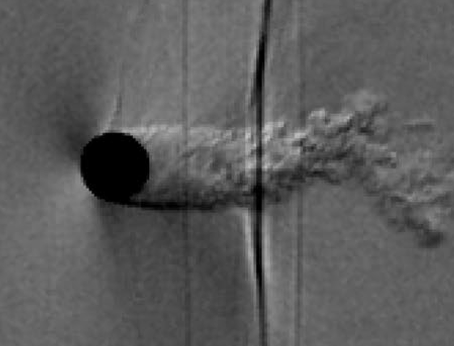
(a) $\mbox{\rm Ma}_{p}=0.9$

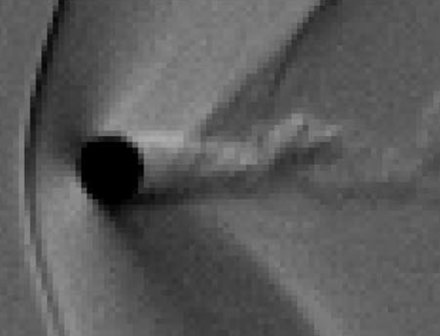
(b) $\mbox{\rm Ma}_{p}=1.21$

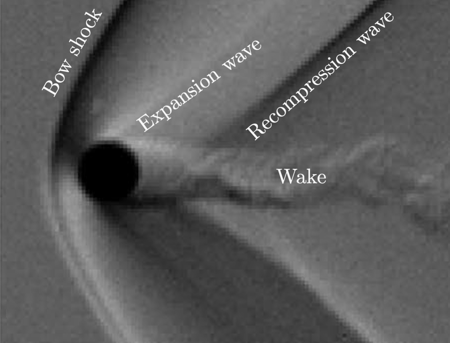
(c) $\mbox{\rm Ma}_{p}=1.39$

Figure 5: Schlieren visualization of flow past a sphere with $\mbox{\rm Re}_{p}=\mathcal{O}\left(10^{5}\right)$. Adapted from Nagata et al. (2020a) with permission.

With the advent of high-performance computing, DNS of compressible particle-laden flows is beginning to shed new light on this topic. Nagata et al. (2016, 2020b) performed DNS of flow past an isolated sphere for $0.3\leq\mbox{\rm Ma}_{p}\leq 2$ and $250\leq\mbox{\rm Re}_{p}\leq 1000$. They report shortcomings of existing drag correlations owing to the compromised accuracy in the transitional regime ($0.9<\mbox{\rm Ma}_{p}<1$) due to lack of experimental data. They demonstrated that the effect of $\mbox{\rm Ma}_{p}$ and $\mbox{\rm Re}_{p}$ on the flow structure and drag coefficient can be characterized by the position of the separation point. A rapid extension of the length of the recirculation region was observed in the transitional regime, where $C_{D}$ was shown to increase with increasing Mach number independently of the Reynolds number.

Shortly after, Loth et al. (2021) combined the DNS data of Nagata et al. (2016, 2020b) with rarefied-gas simulations and an expanded experimental dataset to develop new empirical models for the drag coefficient (given in A.6). It is simpler than that originally proposed by Loth (2008) and appears to be the most accurate and comprehensive model developed for compressible gas–particle flows to date (and the first to incorporate numerical data). It was shown to be approximately twice as accurate compared to the correlations of Loth (2008) and Parmar et al. (2010) at moderate Mach numbers, and showed improvement to Loth’s original model at higher Mach numbers ($\mbox{\rm Ma}_{p}>2$) and for rarefied conditions. The overall trends in $C_{D}$ are shown in Fig. 6, highlighting the quasi-nexus that separates the rarefaction and compressibility flow regimes. It can be seen that the compression-dominated region ($\mbox{\rm Re}_{p}>60$) yields an increase in $C_{D}$ as $\mbox{\rm Ma}_{p}$ increases, whereas in the rarefaction-dominated region ($\mbox{\rm Re}_{p}<30$), $C_{D}$ is inversely proportional to $\mbox{\rm Ma}_{p}$. In between these regimes–the quasi-nexus–there exists a weak transonic bump that connects the two. While DNS was used to quantitatively describe this behavior, the authors suggest additional data is warranted to further refine the drag coefficient within the quasi-nexus region.

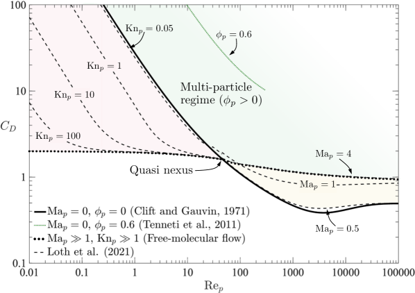
Figure 6: Drag coefficient on a spherical particle showing rarefaction (shaded in red) and compression (shaded in yellow) dominated regimes using the new model proposed by Loth et al. (2021). Multi-particle effects on the drag coefficient are shown in green.

3.2 Drag in multi-particle systems

In the presence of one or more neighbors, the drag force exerted on a particle can vary significantly compared to that of an isolated sphere. Multi-particle drag correlations are needed when the inter-particle distance becomes comparable to the particle diameter–typically when $\phi_{p}\gtrapprox 1\times 10^{-3}$. In a homogeneous fluidization system (see Fig. 7), the single-particle drag coefficient can be corrected to take into account finite volume fraction effects. In general, the mean drag over a suspension of particles has a complex dependency on $\mbox{\rm Re}_{p}$ and $\phi_{p}$ (and likely on $\mbox{\rm Ma}_{p}$ as well, though this is far less studied).

Correlations used to account for the drag force in multi-particle systems can be classified into two types. In the first type, Ergun (1952) proposed a correlation based on the drag force in the limit of Stokes flow with an additional term that depends linearly on $\mbox{\rm Re}_{p}$, such that the drag correction in Eq. (6a) is expressed as

$$F_{D}(\mbox{\rm Re}_{p},\phi_{p})=F_{D}(0,\phi_{p})+\alpha\mbox{\rm Re}_{p}.$$ (10)

Originally, $\alpha$ was only a function of volume fraction (Ergun, 1952). However, it was later shown that $\alpha$ also depends non-linearly on $\mbox{\rm Re}_{p}$ (Hill et al., 2001; Beetstra et al., 2007; Tenneti et al., 2011; Tang et al., 2015). Recently, Tang et al. (2016) proposed a drag law of this type for freely-evolving spherical particles by incorporating the granular temperature (a measure of the particle velocity variance) to account for particle mobility effects (see A.5). They found that particle mobility increases the drag force compared to stationary particles at the same volume fraction, with greater effect at higher $\mbox{\rm Re}_{p}$.

The second correlation type originally proposed by Wen and Yu (1966) takes the form

$$F_{D}(\mbox{\rm Re}_{p},\phi_{p})=F_{D}(\mbox{\rm Re}_{p},0)\phi_{f}^{-\beta},$$ (11)

where $F_{D}(\mbox{\rm Re}_{p},0)$ is the finite Reynolds number drag correction for an isolated particle (see Sec. 3.1). The value for $\beta$ was originally constant (Wen and Yu, 1966), but was later shown to depend on $\mbox{\rm Re}_{p}$ (Di Felice, 1994). More recently, Tenneti et al. (2011) proposed a model following this form based on PR–DNS of flow past random assemblies of fixed spherical particles valid for $0.01\leq\mbox{\rm Re}_{p}\leq 300$ and $0.1\leq\phi_{p}\leq 0.5$ (given in A.4). This was later extended to freely evolving particles for $0.001\leq\rho_{p}/\rho_{f}\leq 1000$ (Tavanashad et al., 2021), where it was shown that $\beta$ depends on the density ratio. Contrary to what Tang et al. (2016) observed, this data showed that the drag force for freely-evolving particles approaches that of fixed particle assemblies when $\rho_{p}/\rho_{f}>100$. Recall $\rho_{p}/\rho_{f}=\mathcal{O}\left(10^{5}\right)$ during PSI.

Compared to incompressible flows, much less attention has been paid to multi-particle drag correlations for flows at finite Mach number. The presence of neighboring particles acts to increase the drag coefficient compared that of an isolated particle. At moderate Reynolds numbers, this increase in drag coefficient obfuscates the quasi-nexus region shown in Fig. 6. A third, multi-particle dominated regime exists in the upper-right quadrant of Fig. 6, located above the Clift and Gauvin (1971) curve. This may intersect with the compression-dominated regime, though its precise behavior remains largely unknown.

In an attempt to incorporate volume fraction effects into compressible drag correlations, Ling et al. (2012) combined the Mach number-dependent drag model of Parmar et al. (2010) with the (incompressible) volume fraction correction of Sangani et al. (1991). Note this follows the second correlation type given by Eq. (11). The corresponding drag coefficient is given by

$$C_{D}(\mbox{\rm Re}_{p},\mbox{\rm Ma}_{p},\phi_{p})=C_{D,{\rm std}}(\mbox{\rm Re}_{p})\xi_{1}(\mbox{\rm Re}_{p},\mbox{\rm Ma}_{p})\xi_{2}(\phi_{p}),$$ (12)

where $\xi_{1}(\mbox{\rm Re}_{p},\mbox{\rm Ma}_{p})$ is the Mach number correlation for an isolated particle that was provided in Eq. (9), and the volume fraction correction is given by

$$\xi_{2}(\phi_{p})=\frac{1+2\phi_{p}}{\left(1-\phi_{p}\right)^{2}}.$$ (13)

The above expression was analytically derived from periodic arrays of spherical particles in the zero Reynolds number limit for $\phi_{p}\leq 0.3$ (Sangani et al., 1991). However, such an approach does not guarantee it will capture the non-linear coupling between $\mbox{\rm Re}_{p}$, $\mbox{\rm Ma}_{p}$, and $\phi_{p}$ in general. Recent PR–DNS of shock-particle interactions have shown that particles experience a large variation in drag force due to fluid-mediated particle-particle interactions, which current models fail to capture (Mehta et al., 2018, 2019b; Osnes and Vartdal, 2021).

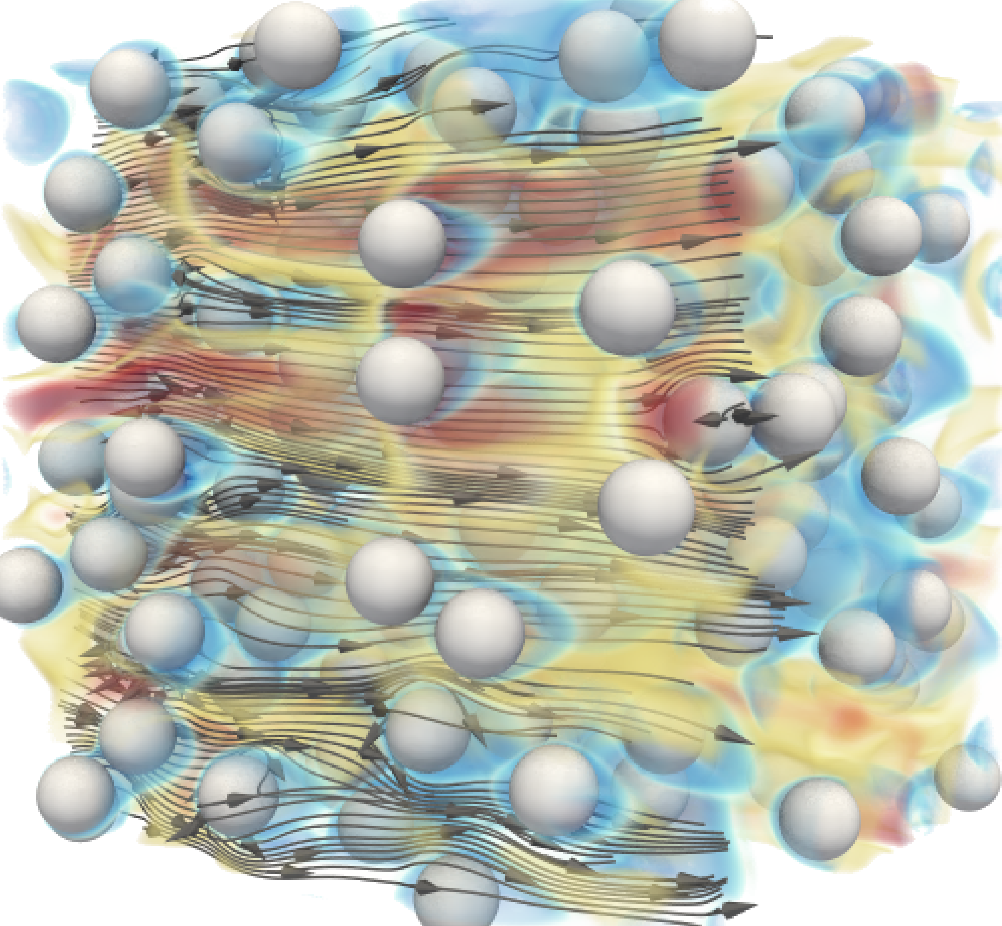
(a) $\mbox{\rm Re}_{p}=20$, $\phi_{p}=0.1$, $\mbox{\rm Ma}_{p}=0$

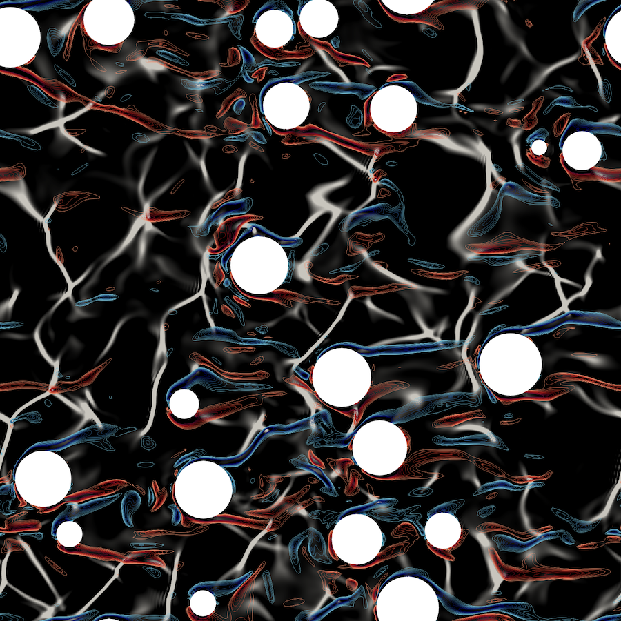
(b) $\mbox{\rm Re}_{p}=300$, $\phi_{p}=0.1$, $\mbox{\rm Ma}_{p}=0.8$

Figure 7: Instantaneous snapshots from PR–DNS of a homogeneous suspension of particles. (a) Incompressible flow with $\rho_{p}/\rho_{f}=1000$ showing fluid velocity (red: high, blue: low) (Lattanzi et al., 2021a). (b) Compressible flow past fixed spheres showing a 2D cross-section of the 3D flow highlighting fluid dilatation (black/white) and vorticity (red: positive, blue: negative) (Khalloufi, 2021).

While PR–DNS of multi-particle systems are now common for incompressible flow, only in recent years PR–DNS of compressible flows past assemblies of particles have come online (e.g., Regele et al., 2014; Mehta et al., 2016, 2018; Theofanous et al., 2018; Hosseinzadeh-Nik et al., 2018; Osnes et al., 2019; Shallcross et al., 2020). However, these studies typically consider a shock wave traveling through an array of particles, which introduces challenges in developing drag correlations due to the lack of statistical stationarity and homogeneity. Figure 7(b) shows an example of PR–DNS of a homogeneous flow with $\phi_{p}=0.1$ and $\mbox{\rm Ma}_{p}=0.8$ based on the mean slip velocity (Khalloufi, 2021). The flow accelerates to supersonic speeds in the interstitial space between particles, resulting in large values of fluid dilatation (shocklets). These regions of high compression have important consequences on vorticity generation due to baroclinic torque ($\nabla\rho_{f}\times\nabla p_{f}$) at the vertex of curved shocks (Kida and Orszag, 1990), which is anticipated to alter the drag force. This work among other recent PR–DNS represent a promising new direction for developing improved drag correlations that span relevant values of $\mbox{\rm Re}_{p}$, $\mbox{\rm Ma}_{p}$, and $\phi_{p}$ for applications related to PSI and other compressible gas–particle flows.

3.3 Unsteady inviscid force

Compared to the quasi-steady drag force, the unsteady forces appearing in Eq. (6) have received much less attention, especially in the context of compressible flows. It is typically assumed that these terms scale with the fluid-to-particle density ratio, and therefore can be neglected for gas–solid flows. This is generally true for the case of a particle accelerating in a quiescent fluid. However, when the surrounding fluid is accelerating, the order of magnitude of the inviscid unsteady terms ($\mbox{\boldmath{$F$}}_{iu}$ and $\mbox{\boldmath{$F$}}_{un}$) relative to the quasi-steady drag force scales like $\mbox{\rm Re}_{p}d_{p}/L_{f}$, where $L_{f}$ is the characteristic length scale of the background flow (Bagchi and Balachandar, 2002). Therefore, the motion of finite-size particles in a compressible flow undergoing strong acceleration (e.g., in the presence of a shock wave) can be greatly influenced by the unsteady forces, regardless of the density ratio. In fact, the peak drag coefficient of an isolated particle interacting with a shock wave can be more than 10 times larger than the value from the quasi-steady drag force depending on the shock Mach number, $\mbox{\rm Ma}_{s}$, and $\mbox{\rm Re}_{p}$ (Parmar et al., 2009; Ling et al., 2011).

The inviscid unsteady force given in Eq. (6c) is expressed in terms of a response kernel, $K_{iu}(\tau;\mbox{\rm Ma}_{p})$, used to weigh the history of the particle’s acceleration. The kernel decays over a non-dimensional acoustic time $ct/d_{p}$, which depends on both the particle’s shape and Mach number. In an incompressible flow, the acoustics propagate infinitely fast and the kernel reduces to a Dirac delta function, i.e., $K_{iu}(\tau;\mbox{\rm Ma}_{p}=0)=\delta(\tau)/2$. For a spherical particle in an incompressible flow, integration of the kernel results in an added mass coefficient $C_{m}=0.5$. However, when the flow is compressible, the Mach number delays the approach to steady state and the force no longer takes the form of a constant mass multiplied by the instantaneous acceleration. Because of this, Miles (1951); Longhorn (1952) and later reiterated by Parmar et al. (2008), emphasized that reference to this force as a ‘virtual’ or ‘added’ mass is only applicable to incompressible flows.

A popular expression for $K_{iu}$ was obtained by Longhorn (1952) for a spherical particle in the limit of zero Mach number as $K_{iu}(\tau;\mbox{\rm Ma}_{p}=0)=\exp(-\tau)\cos(\tau)$. More than half a century later, Parmar et al. (2008) extended this to finite (but subcritical) Mach numbers. They demonstrated that $\mbox{\rm Ma}_{p}$ has a pronounced effect on both the peak value of the unsteady force and the effective added-mass coefficient. By employing the compressible form of the Bernoulli equation, a Mach number expansion for pressure was derived and integrated around a sphere to obtain the force. At a Mach number of $0.5$, the effective added-mass coefficient was found to be $C_{m}(\mbox{\rm Ma}_{p}=0.5)\approx 1$, approximately twice as large as the incompressible value for a sphere.

In general, $K_{iu}$ becomes negligibly small after a few acoustic time scales. If the relative acceleration changes slowly over this duration, it can be taken outside of the integral and Eq. (6c) can be rewritten as

$$\mbox{\boldmath{$F$}}_{iu}\approx V_{p}C_{m}(\mbox{\rm Ma}_{p},\phi_{p})\left(\frac{{\rm D}(\rho_{f}\mbox{\boldmath{$u$}}_{f})}{{\rm D}t}-\frac{{\rm d}(\rho_{f}\mbox{\boldmath{$v$}}_{p})}{{\rm d}t}\right),$$ (14)

where $V_{p}$ is the particle volume. Ling et al. (2012) proposed a model for the added mass coefficient, given by

$$C_{m}(\mbox{\rm Ma}_{p},\phi_{p})=C_{M,{\rm std}}\eta_{1}(\mbox{\rm Ma}_{p})\eta_{2}(\phi_{p}),$$ (15)

which reduces to the usual value $C_{M,{\rm std}}=0.5$ in the limit of zero Mach number and volume fraction. The Mach number correction (valid in the subcritial regime) is given by (Parmar et al., 2008)

$$\eta_{1}(\mbox{\rm Ma}_{p})=\begin{cases}1+1.8\mbox{\rm Ma}_{p}+7.6\mbox{\rm Ma}_{p}^{4}&\text{if }\mbox{\rm Ma}_{p}<0.6,\\ 2.633&\text{otherwise}.\end{cases}$$ (16)

The volume fraction correction is taken from the expression by Sangani et al. (1991) as

$$\eta_{2}(\phi_{p})=\frac{1+2\phi_{p}}{1-\phi_{p}},$$ (17)

which is valid for random arrays of spheres in incompressible low Reynolds number flow when $\phi_{p}<0.3$. Such a simple expression for the inviscid unsteady force has received mixed success when applied to shock-particle interactions (Parmar et al., 2009; Koneru and Balachandar, 2021; Osnes and Vartdal, 2021).

An interesting alternative to modeling the inviscid unsteady force was recently proposed by Fox et al. (2020), and demonstrated to be a key ingredient in restoring hyperbolicity of the compressible two-fluid equations (refer back to Sec. 2.2). In-lieu of treating the force as a separate term in Eq. (5), the added mass is transported with the particle velocity, which implicitly captures the force history without the need for a response kernel. This is based on the formulation of Cook and Harlow (1984), but generalized to a compressible fluid and a non-constant added-mass function to capture volume fraction effects. The mass appearing in the conservation equations are augmented to include the portion of the wake moving with the particle. In an EE framework, this involves replacing $\phi_{p}$ in the particle-phase equations with $\phi_{p}^{\star}=\phi_{p}+\phi_{a}$, such that the particles carry an added mass $m_{p}=(\rho_{p}\phi_{p}+\rho_{f}\phi_{a})V_{p}=\rho_{e}\phi_{p}^{\star}V_{p}$, where $\alpha_{a}$ is the added volume fraction of the surrounding fluid and $\rho_{e}$ is the effective density of the particle. A simple model was proposed based on a mass exchange function that acts as a source term for $\phi_{p}^{\star}$, given by

$$\frac{\partial\rho_{e}\phi_{p}^{\star}}{\partial t}+\nabla\boldsymbol{\mbox{\boldmath{$\cdot$}}}\left(\rho_{e}\phi_{p}^{\star}\mbox{\boldmath{$u$}}_{p}\right)=\frac{\rho_{f}\phi_{f}\phi_{p}}{\tau_{a}}\left(C_{m}^{\star}-C_{m}\right),$$ (18)

where $\tau_{a}$ is a time scale that characterizes the expansion/contraction/formation of particle wakes, and $C_{m}^{\star}$ is the added mass function that should depend on $\mbox{\rm Re}_{p}$, $\mbox{\rm Ma}_{p}$, and $\phi_{p}$. When a particle moves from a region of high $\phi_{p}$ to low $\phi_{p}$ (i.e., into a region with larger inter-particle spacing), $C_{m}<C_{m}^{\star}$ and the wake will grow by entraining the surrounding fluid. In a EL framework, this would require replacing $m_{p}$ in Eq. (5) with an effective mass $m_{p}^{\star}$ carried by each particle that evolves according to

$$\frac{{\rm d}m_{p}^{\star}}{{\rm d}t}=\frac{1}{\tau_{a}}\rho_{f}\phi_{f}V_{p}(C_{m}^{\star}-C_{m}).$$ (19)

Such a treatment for the added mass has advantages over the more traditional approach given by Eq. (6c), as the instantaneous acceleration of each phase need not be evaluated at the particle location, and the time-history of the response kernel is not required. Models for $\tau_{a}$ and $C_{m}^{\star}$ are needed for relevant values of $\mbox{\rm Re}_{p}$, $\mbox{\rm Ma}_{p}$, and $\phi_{p}$, which could be evaluated from PR–DNS (e.g., see Moore and Balachandar, 2019, for a recent evaluation of $\tau_{a}$).

4 Pseudo-turbulence in multi-particle systems

Flow through a collection of particles gives rise to wakes that interact non-linearly with each other and with surrounding particles. The collective effect of these flow disturbances acts as a source of fluid-phase turbulence. Because such fluctuations exist even in laminar flow (e.g., via steady wakes), and originate at small scales, it is often termed pseudo-turbulence. This is in contrast to classical turbulence that involves a transfer of energy from large scales of motion to small scales. Models for velocity fluctuations originating from pre-existing background turbulence (i.e., from the classical turbulence cascade) are not considered here as they have already received significant attention for single-phase flow (e.g., Garnier et al., 2009). Instead, we focus on models for the pseudo-turbulent Reynolds stress, $\mbox{\boldmath{$R$}}_{f}$ in Eqs. (3)–(4), that is expected to play a role when the inter-particle spacing is comparable to the size of the wakes (i.e., at moderate values of $\phi_{p}$).

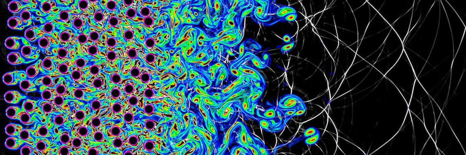
Figure 8: A two-dimensional simulation showing gas-phase vorticity (color) and dilatation (black/white) shortly after a planar shock wave passes over a suspension of particles with $\mbox{\rm Ma}_{s}=1.22$ and $\phi_{p}=0.17$. Adapted from Shallcross et al. (2020).

When a shock wave passes over a cloud of particles at moderate volume fractions, small-scale velocity fluctuations are produced in particle interstitial sites and advected downstream with the mean flow (see Fig. 8). Theofanous et al. (2018) performed one of the first three-dimensional particle-resolved simulations of shock-induced dispersion. The gas phase was shown to choke near the downstream edge of the particle cloud due to the abrupt change in volume fraction, resulting in supersonic expansion that significantly increases particle acceleration. Shallcross et al. (2020) later showed that including $\mbox{\boldmath{$R$}}_{f}$ in the definition of total fluid energy is critical for capturing this choking behavior in simulations based on averaged equations. Near the edge of the particle cloud, large gradients in $\mbox{\boldmath{$R$}}_{f}$ can be on the same order as the forces acting on the particles (Osnes et al., 2019). The corresponding root-mean-square velocity fluctuations have been observed to be as much as 60% of the mean flow. Its strength increases with increasing values of $\phi_{p}$ and incident shock Mach number (Mehta et al., 2019a; Osnes et al., 2019).

Modeling the pseudo-turbulent Reynolds stress has only gained considerable attention in recent years. An algebraic model for the pseudo-turbulent kinetic energy (PTKE), $k_{f}={\rm tr}(\mbox{\boldmath{$R$}}_{f})/2$, was first proposed by Mehrabadi et al. (2015) for incompressible homogeneous gas–solid flows, given by

$$\frac{k_{f}}{K_{f}}=2\phi_{p}+2.5\phi_{p}\phi_{f}^{3}\exp\left(-\phi_{p}\mbox{\rm Re}_{p}^{1/2}\right),$$ (20)

where $K_{f}=\mbox{\boldmath{$u$}}_{f}\boldsymbol{\mbox{\boldmath{$\cdot$}}}\mbox{\boldmath{$u$}}_{f}/2$ is the kinetic energy of the resolved flow field. The correlation was developed in the range $0.1\leq\phi_{p}\leq 0.5$ and $0.01\leq\mbox{\rm Re}_{p}\leq 300$ and tends to appropriate values in the zero volume fraction limit (i.e., $k_{f}\rightarrow 0$ when $\phi_{p}\rightarrow 0$). The pseudo-turbulent Reynolds stress tensor is reconstructed from the PTKE according to

$$\mbox{\boldmath{$R$}}_{f}^{\prime}=2\rho_{f}k_{f}\left(\mbox{\boldmath{$b$}}+\frac{1}{3}\mathbb{I}\right),$$ (21)

where $\mbox{\boldmath{$R$}}_{f}^{\prime}$ is the Reynolds stress aligned with the local velocity difference between the phases and $b$ is the anisotropic stress tensor that depends on $\mbox{\rm Re}_{p}$ and $\phi_{p}$ (Mehrabadi et al., 2015). $\mbox{\boldmath{$R$}}_{f}$ is then obtained by rotating $\mbox{\boldmath{$R$}}_{f}^{\prime}$ to align with the Cartesian coordinate system. Details on the implementation of the rotation matrix in an EE framework can be found in Peng et al. (2019).

Using PR–DNS of shock-induced flow through random arrays of particles, Osnes et al. (2019) proposed a model for the streamwise component of the Reynolds stress (denoted here as direction $1$) according to

$$R_{f,11}=u_{f,1}^{2}\frac{\phi_{\rm sep}}{\phi_{f}-\phi_{\rm sep}},$$ (22)

where $\phi_{\rm sep}$ represents the volume fraction of separated flow in particle wakes, which increases significantly as $\phi_{p}$ is reduced as a result of increasing inter-particle separation. The authors proposed a simple model of the form $\phi_{\rm sep}\left(\phi_{f},\mbox{\rm Re}_{p}\right)=\phi_{p}C\left(\mbox{\rm Re}_{p}\right)$, where $C\left(\mbox{\rm Re}_{p}\right)\approx 1.5$ was determined for incident shock Mach numbers between $2.2\leq\mbox{\rm Ma}_{s}\leq 3$ and volume fractions $0.05\leq\phi_{p}\leq 0.1$. The authors note that it would be appropriate to introduce a time-dependency for $\phi_{\rm sep}$, since particle wakes and fluctuations are not generated instantaneously after the shock wave passes over a particle. This is conceptually similar to the added mass formulation proposed by Fox et al. (2020) reported in Sec. 3.3. However, such models do not yet exist.

A key drawback with the algebraic models proposed by Mehrabadi et al. (2015) and Osnes et al. (2019) is that they only predict finite PTKE in the regions where particles are present ($\phi_{p}>0$). While these fluctuations originate in the vicinity of particles, they can be transported with the mean flow into regions devoid of particles where $\phi_{p}=0$ (see Fig. 8). Another challenge is distinguishing the sub-grid scale velocity fluctuations originating from pre-existing turbulence (via a classical energy cascade) and those induced by particles (pseudo turbulence). With this in mind, Shallcross et al. (2020) rigorously derived a transport equation for the PTKE based on volume filtering, given by

$$\frac{\partial\phi_{f}\rho_{f}k_{f}}{\partial t}+\nabla\boldsymbol{\mbox{\boldmath{$\cdot$}}}\left(\phi_{f}\rho_{f}\mbox{\boldmath{$u$}}_{f}k_{f}\right)=-\phi_{f}\mbox{\boldmath{$R$}}_{f}\boldsymbol{\mbox{\boldmath{$:$}}}\nabla\mbox{\boldmath{$u$}}_{f}+\left(\mbox{\boldmath{$u$}}_{p}-\mbox{\boldmath{$u$}}_{f}\right)\boldsymbol{\mbox{\boldmath{$\cdot$}}}\mbox{\boldmath{$F$}}_{p}-\phi_{f}\rho_{f}\varepsilon_{PT},$$ (23)

where the viscous and sub-filtered contributions are absorbed into $\varepsilon_{PT}$, which represents dissipation of PTKE. The first term on the right-hand side of Eq. (23) represents production due to mean shear–the usual turbulence production term in single phase flow. The second term on the right-hand side represents production due to particle drag that is only active when $\phi_{p}>0$. It was found that reconstructing $\mbox{\boldmath{$R$}}_{f}$ from the transported PTKE via Eq. (21) yields accurate predictions of the anisotropy for shock-particle interactions, despite the coefficients being derived for steady, incompressible flows. However, the results were shown to depend strongly on $\varepsilon_{PT}$.

Following what is typically done in single-phase turbulence modeling (Vassilicos, 2015), the dissipation rate can be modeled as $\varepsilon_{PT}\propto k_{f}/\tau_{\varepsilon}$, where $\tau_{\varepsilon}$ is a dissipation time scale that requires modeling. Vartdal and Osnes (2018) proposed a simple model of the form $\tau_{\varepsilon}=l/\sqrt{k_{f}}$, where the length scale $l$ can be related to $d_{p}$ or the inter-particle spacing. Shallcross et al. (2020) proposed a model that blends two time scales: one similar to the model by Vartdal and Osnes (2018) away from particles; and another based on the relative velocity between the phases in the vicinity of particles. However, the model has only been tested under limited flow conditions. For broader applicability, a transport equation for the dissipation rate could be derived as well. Such an approach would of course lead to additional terms that require models. The increase in available compressible DNS data in recent years (e.g., Theofanous and Chang, 2017; Theofanous et al., 2018; Mehta et al., 2019a; Shallcross et al., 2020) represent an exciting opportunity for developing such models valid across relevant two-phase flow conditions.

5 Conclusions

Above we present a survey of available models for high-speed gas–particle flows, with an emphasis on fluid-particle interactions. This class of flows gives rise to rich multiphase flow physics that pose significant challenges in predicting its behavior. While such flows are present in numerous applications, this article was primarily motivated by PSI during planetary and lunar landings. With future planned sample-return missions from Mars and eventual crewed missions to the Moon, Mars, and beyond, the risks associated with PSI are paramount. Simulating the harsh environment during touchdown using physics-based (EE and EL) approaches offers many advantages over the use of empirical correlations for macroscopic behavior like crater depth and erosion rate. However, the subgrid-scale models they rely on are largely based on data from incompressible flows or outdated experimental measurements.

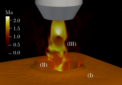
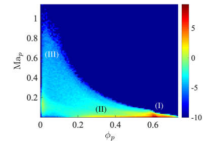
Figure 9: EL simulation of an underexpanded jet impinging on a granular bed highlighting the surface (I), crater (II), and ejecta (III). (a) Visualization of the granular surface ($\phi_{p}=0.6$ contour shown in brown) and local gas-phase Mach number (red/yellow). (b) Joint-PDF (in log scale) of particle Mach number and volume fraction at the same instant. Adapted from Shallcross (2021).

It should be noted that when the particle phase is densely packed (i.e., near close packing $\phi_{p}>0.6$), a significant amount of power would be required to sustain a mean velocity difference between the phases at moderate Mach numbers. To highlight this, Fig. 9 shows results from a recent EL simulation of an underexpanded jet impinging on a bed of monodisperse spherical particles (Shallcross, 2021). The joint probability density function (PDF) of $\mbox{\rm Ma}_{p}$ and $\phi_{p}$ reveals high probability events of moderate Mach numbers at low $\phi_{p}$ (corresponding to the ejecta above the crater), whereas $\phi_{p}>0.4$ predominantly occurs when $\mbox{\rm Ma}_{p}<0.1$. Thus, it might be possible to restrict model development at finite Mach numbers to dilute and moderately dense concentrations only.

Finally, it should be noted that much of the flow physics discussed throughout this review are also present in many systems on Earth. For example, pyroclastic density currents are dangerous multiphase flows emanating from volcanic eruptions that operate under a wide range of Mach numbers and volume fractions (Lube et al., 2020). In addition, the detonation of a heterogeneous explosive results in rapid dispersal of high-speed solid particles (Zhang et al., 2001), which can have tragic consequences as seen with the 2020 Beirut explosion (Guglielmi, 2020).

Appendix A Some common drag coefficients

In this Appendix, various correlations for the drag coefficient are provided as Matlab functions, along with their range of validity and general comments.

A.1 Clift and Gauvin (1971)

Validity	Comment
$\mbox{\rm Re}_{p}<2\times 10^{5}$	Standard Reynolds number-dependent drag coefficient used for an isolated particle in incompressible flow. Reduces to the classical Schiller–Naumann correlation at moderate Reynolds numbers and to Stokes drag when $\mbox{\rm Re}_{p}\rightarrow 0$.
$\mbox{\rm Ma}_{p}=0$
$\phi_{p}=0$

⬇

1ction CD = Clift_Gauvin(Rep)

2CD = 24 / Rep * (1 + 0.15 * Rep^(0.687)) + 0.42 / (1 + 42500 / Rep^(1.16));

3end

A.2 Henderson (1976)

Validity	Comment
$\mbox{\rm Re}_{p}<2\times 10^{4}$	In addition to the usual Reynolds and Mach number based on the relative velocity, the drag correlation is also a function of the Reynolds and Mach number based on the freestream velocity, $\mbox{\rm Re}_{\infty}$ and $\mbox{\rm Ma}_{\infty}$. It also includes effects of the temperature ratio between the gas and particle $T_{p}/T_{f}$.
$\mbox{\rm Ma}_{p}<6$
$\phi_{p}=0$

⬇

1ction CD = Henderson(Rep,Map,Re_inf,Ma_inf,Tf,Tp)

2global gamma

3S=Map*sqrt(0.5*gamma);

4S_inf=MaInf*sqrt(0.5*gamma);

5if Ma $\leq$ 1

6 CD = 24 / (Rep + Map*sqrt(0.5*gamma)*(4.33 + (3.65 - 1.53*(Tp/Tf))/(1 + 0.353*(Tp/Tf))) * exp(-0.247*Rep/(S)))+ exp(-0.5*Map/sqrt(Rep))*((4.5 + 0.38 * (0.03*Rep + 0.48*sqrt(Rep))) / (1 + 0.03*Rep + 0.48*sqrt(Rep)) + 0.1*Map^2 + 0.2*Map^8) + (1 - exp(-1*Map/Rep)) * 0.6 * S;

7elseif Map > 1 && Map < 1.75

8 CD = (24 / (Rep + sqrt(0.5*gamma) * (4.33 + (3.65 - 1.53*(Tp/Tf)) / (1 + 0.353*(Tp/Tf))) * exp(-0.247*Rep / (sqrt(0.5*gamma)))) + exp(-0.5*1/sqrt(Rep)) * ((4.5 + 0.38 * (0.03*Rep + 0.48*sqrt(Rep))) / (1 + 0.03*Rep + 0.48*sqrt(Rep))+ 0.1*1^2 + 0.2*1^8) + (1 - exp(-1/Rep)) * 0.6 * sqrt(0.5*gamma)) + 4/3 * (Ma_inf - 1) * ((0.9 + 0.34/1.75^2 + 1.86 * sqrt(1.75/Re_inf) * (2 + 2/(1.75*sqrt(0.5*gamma))^2+ 1.058 / (1.75*sqrt(0.5*gamma)) * sqrt(Tp/Tf) - 1 / (1.75*sqrt(0.5*gamma))^4)) / (1 + 1.86 * sqrt(1.75/Re_inf)) - (24 / (Rep + sqrt(0.5*gamma) * (4.33 + (3.65 - 1.53*(Tp/Tf)) / (1 + 0.353*(Tp/Tf))) * exp(-0.247*Rep/(sqrt(0.5*gamma)))) + exp(-0.5*1/sqrt(Rep))*((4.5 + 0.38 * (0.03*Rep + 0.48*sqrt(Rep))) / (1 + 0.03*Rep + 0.48*sqrt(Rep))+ 0.1*1^2 + 0.2*1^8) + (1 - exp(-1/Rep)) * 0.6 * sqrt(0.5*gamma)));

9else

10 CD = (0.9 + 0.34/Ma_inf^2 + 1.86 * sqrt(Ma_inf/Re_inf) * (2 + 2/(S_inf)^2 + 1.058/(S_inf) * sqrt(Tp/Tf) - 1/(S_inf)^4))/ (1 + 1.86 * sqrt(Ma_inf/Re_inf));

11

12end

13end

A.3 Parmar et al. (2010)

Validity	Comment
$\mbox{\rm Re}_{p}\leq 2\times 10^{5}$	The original paper (Parmar et al., 2010) contains a typo, the correct formulation can be found in the subsequent thesis (Parmar, 2010). The original correlation was developed for an isolated particle, Ling et al. (2012) added a correction for $0\leq\phi_{p}\leq 0.3$.
$\mbox{\rm Ma}_{p}\leq 1.75$
$\phi_{p}=0$

⬇

1ction CD = Parmar(Rep,Map,phip)

2fsub=zeros(1,3);

3fsup=zeros(1,3);

4Csup=zeros(1,3);

5Csub=zeros(1,3);

6

7Mcr = 0.6;

8CDMcr = 24 / Rep * (1 + 0.15 * Rep^(0.684)) + 0.513 / (1 + 483 / Rep^(0.669));

9CDM1 = 24 / Rep * (1 + 0.118 * Rep^(0.813)) + 0.69 / (1 + 3550 / Rep^(0.793));

10CDM175 = 24 / Rep * (1 + 0.107 * Rep^(0.867)) + 0.646 / (1 + 861 / Rep^(0.634));

11

12if Map $\leq$ Mcr

13 % Subcritical regime (standard drag of Clift and Gauvin)

14 CDstd = 24 / Rep * (1 + 0.15 * Rep^(0.687)) + 0.42 / (1 + 42500 / Rep^(1.16));

15 CD = CDstd + (CDMcr - CDstd) * Map / Mcr;

16elseif Map>Mcr && Map$\leq$1

17 % Intermediate regime (supercritical and subsonic)

18 Csub(1) = 6.48; Csub(2) = 9.28; Csub(3) = 12.21;

19 fsub(1) = -0.087 + 2.92*Map - 4.75*Map^2 + 2.83*Map^3;

20 fsub(2) = -0.12 + 2.66*Map - 4.36*Map^2 + 2.53*Map^3;

21 fsub(3) = 1.84 - 5.13*Map + 6.05*Map^2 - 1.91*Map^3;

22 fsubM1(1) = 0.913; fsubM1(2) = 0.71; fsubM1(3) = 0.85;

23 fsubMcr(1) = 0.56628; fsubMcr(2) = 0.45288; fsubMcr(3) = 0.52744;

24 zsub = ...

25 (fsub(1) - fsubMcr(1)) / (fsubM1(1) - fsubMcr(1)) * (log(Rep) - Csub(2))/(Csub(1)-Csub(2)) * (log(Rep)-Csub(3))/(Csub(1)-Csub(3)) + ...

26 (fsub(2) - fsubMcr(2)) / (fsubM1(2) - fsubMcr(2)) * (log(Rep) - Csub(1))/(Csub(2)-Csub(1)) * (log(Rep)-Csub(3))/(Csub(2)-Csub(3)) + ...

27 (fsub(3) - fsubMcr(3)) / (fsubM1(3) - fsubMcr(3)) * (log(Rep) - Csub(1))/(Csub(3)-Csub(1)) * (log(Rep)-Csub(2))/(Csub(3)-Csub(2));

28 CD = CDMcr + (CDM1 - CDMcr) * zsub;

29elseif Map > 1 && Map<1.75

30 % Supersonic regime

31 Csup(1) = 6.48; Csup(2) = 8.93; Csup(3) = 12.21;

32 fsup(1) = 0.126 + 1.15*Map - 0.306*Map^2 - 0.007*Map^3 - 0.061*exp((1-Map)/0.011);

33 fsup(2) = -0.901 + 2.93*Map - 1.573*Map^2 + 0.286*Map^3 - 0.042*exp((1-Map)/0.01);

34 fsup(3) = 0.13 + 1.42*Map - 0.818*Map^2 + 0.161*Map^3 - 0.043*exp((1-Map)/0.012);

35 fsupM1(1) = 0.902; fsupM1(2) = 0.7; fsupM1(3) = 0.85;

36 fsupM175(1) = 1.163859375; fsupM175(2) = 0.94196875; fsupM175(3) = 0.972734375;

37 zsup = ...

38 (fsup(1) - fsupM1(1)) / (fsupM175(1) - fsupM1(1)) * ...

39 (log(Rep) - Csup(2))/(Csup(1)-Csup(2)) * (log(Rep)-Csup(3))/(Csup(1)-Csup(3)) + ...

40 (fsup(2) - fsupM1(2)) / (fsupM175(2) - fsupM1(2)) * ...

41 (log(Rep) - Csup(1))/(Csup(2)-Csup(1)) * (log(Rep)-Csup(3))/(Csup(2)-Csup(3)) + ...

42 (fsup(3) - fsupM1(3)) / (fsupM175(3) - fsupM1(3)) * ...

43 (log(Rep) - Csup(1))/(Csup(3)-Csup(1)) * (log(Rep)-Csup(2))/(Csup(3)-Csup(2));

44 CD = CDM1 + (CDM175 - CDM1) * zsup;

45 else

46 % Map > 1.75 is outside validity

47 disp('Map>1.75 not valid')

48end

49

50% Correct for volume fraction (Sangani et al., 1991)

51CD = CD * (1 + 2 * phip) / (1 - phip)^2;

52end

A.4 Tenneti et al. (2011)

Validity	Comment
$0.01\leq\mbox{\rm Re}_{p}<300$	Developed using PR–DNS of homogeneous flow past random assemblies of fixed spherical particles. Refinement using freely-evolving particles with $0.001\leq\rho_{p}/\rho_{f}\leq 1000$ can be found in Tavanashad et al. (2021). The correlation for freely-evolving particles approaches that of fixed particle assemblies when $\rho_{p}/\rho_{f}>100$. Note there is a difference in a factor $(1-\phi_{p})$ from the original paper (Tenneti et al., 2011) in order to remove the average pressure gradient used to force the flow.
$\mbox{\rm Ma}_{p}=0$
$0.1\leq\phi_{p}\leq 0.5$

⬇

1ction CD = Tenneti(Rep,phip)

2b1 = 5.81*phip/(1-phip)^3+0.48*phip^(1/3)/(1-phip)^4;

3b2 = phip^3*Rep*(0.95+0.61*phip^3/(1-phip)^2);

4F = (1-phip) * ((1+0.15*Rep^(0.687))/(1-phip)^3+b1+b2);

5CD=24*F/Rep;

6end

A.5 Tang et al. (2016)

Validity	Comment
$40\leq\mbox{\rm Re}_{p}<1000$	Developed using PR–DNS of flow past freely-evolving spherical particles with elastic collisions. In addition to the usual Reynolds number, the drag correlation depends on a Reynolds number based on the granular temperature $\Theta_{p}$, $\mbox{\rm Re}_{T}=\rho_{f}\sqrt{\Theta_{p}}d_{p}/\mu_{f}$, to account for the effect of particle mobility. The contribution of particle mobility is accounted for though the force deviation $\Delta F_{D}=2.98\mbox{\rm Re}_{T}\phi_{p}/(1-\phi_{p})^{2}$. This is combined with the drag for static array of particles proposed by Tang et al. (2015).
$\mbox{\rm Ma}_{p}=0$
$0.1\leq\phi_{p}\leq 0.45$
$\rho_{p}/\rho_{f}>500$

⬇

1ction CD = Tang(Rep,phip,Re_T)

2F = 10*phip/(1-phip)^2 + (1-phip)^2 * (1+1.5*sqrt(phip)) + (0.11*phip*(1+phip) - 0.00456/(1-phip)^4 + (0.169*(1-phip) + 0.0644/(1-phip)^4) * Rep^(-0.343)) * Rep + 2.98*Re_T * phip/(1-phip)^2;

3CD=24*F/Rep;

4end

A.6 Loth et al. (2021)

Validity	Comment
$\mbox{\rm Re}_{p}\leq 2\times 10^{5}$	A refinement of the popular Loth (2008) drag correlation using an expanded experimental dataset along with DNS of (continuum) supersonic flow past a sphere and rarefied gas simulations via direct simulation Monte Carlo (DSMC).
$\mbox{\rm Ma}_{p}<10$
$\phi_{p}=0$

⬇

1ction CD = Loth(Rep,Map)

2global gamma

3eps = 1e-12;

4if Rep $\leq$ 45

5 % Rarefraction-dominated regime

6 Knp = sqrt(0.5 * pi * gamma) * Map / Rep;

7 fKn = 1 / (1 + Knp*(2.514 + 0.8*exp(-0.55/Knp)));

8 CD1 = 24 / Rep * (1 + 0.15*Rep^(0.687)) * fKn;

9 s = Map * sqrt(0.5 * gamma);

10 if (Map $\leq$ 1)

11 JM = 2.26 - 0.1/Map + 0.14/Map^3;

12 else

13 JM = 1.6 + 0.25/Map + 0.11/Map^2 + 0.44/Map^3;

14 end

15 CD2 = (1 + 2*s^2) * exp(-s^2) / (s^3*sqrt(pi) + eps) + (4*s^4 + 4*s^2 - 1) * erf(s) / (2*s^4 + eps) + 2 / (3 * s + eps) * sqrt(pi);

16 CD2 = CD2 / (1 + (CD2/JM - 1) * sqrt(Rep/45));

17 CD = CD1 / (1 + Map^4) + Map^4 * CD2 / (1 + Map^4);

18else

19 % Compression-dominated regime

20 if (Map < 1.5)

21 CM = 1.65 + 0.65 * tanh(4*Map - 3.4);

22 else

23 CM = 2.18 - 0.13 * tanh(0.9*Map - 2.7);

24 end

25 if (Map < 0.8)

26 GM = 166*Map^3 + 3.29*Map^2 - 10.9*Map + 20;

27 else

28 GM = 5 + 40*Map^(-3);

29 end

30 if (Map < 1)

31 HM = 0.0239*Map^3 + 0.212*Map^2 - 0.074*Map + 1;

32 else

33 HM = 0.93 + 1 / (3.5 + Map^5);

34 end

35 CD = 24/Rep*(1 + 0.15 * Rep^(0.687))*HM + 0.42*CM / (1+42500/Rep^(1.16*CM) + GM/sqrt(Rep));

36end

37end

References

- Akiki et al. (2016) Akiki, G., Jackson, T., Balachandar, S., 2016. Force variation within arrays of monodisperse spherical particles. Physical Review Fluids 1, 044202.
- Akiki et al. (2017) Akiki, G., Jackson, T., Balachandar, S., 2017. Pairwise interaction extended point-particle model for a random array of monodisperse spheres. Journal of Fluid Mechanics 813, 882–928.
- Anderson and Jackson (1967) Anderson, T.B., Jackson, R., 1967. Fluid mechanical description of fluidized beds. Equations of motion. Industrial & Engineering Chemistry Research 6, 527–539.
- Andreotti et al. (2021) Andreotti, B., Claudin, P., Iversen, J.J., Merrison, J.P., Rasmussen, K.R., 2021. A lower-than-expected saltation threshold at Martian pressure and below. Proceedings of the National Academy of Sciences 118.
- Bagchi and Balachandar (2002) Bagchi, P., Balachandar, S., 2002. Steady planar straining flow past a rigid sphere at moderate reynolds number. Journal of Fluid Mechanics 466, 365–407.
- Bailey and Starr (1976) Bailey, A.B., Starr, R.F., 1976. Sphere drag at transonic speeds and high reynolds numbers. AIAA Journal 14, 1631–1631.
- Balachandar and Eaton (2010) Balachandar, S., Eaton, J., 2010. Turbulent dispersed multiphase flow. Annual Review of Fluid Mechanics 42, 111–133.
- Balakrishnan and Bellan (2018) Balakrishnan, K., Bellan, J., 2018. High-fidelity modeling and numerical simulation of cratering induced by the interaction of a supersonic jet with a granular bed of solid particles. International Journal of Multiphase Flow 99, 1–29.
- Balakrishnan and Bellan (2019) Balakrishnan, K., Bellan, J., 2019. A multi-species modeling framework for describing supersonic jet-induced cratering in a granular bed: Cratering on Titan case study. International Journal of Multiphase Flow 118, 205–241.
- Balakrishnan and Bellan (2021) Balakrishnan, K., Bellan, J., 2021. Fluid density effects in supersonic jet-induced cratering in a granular bed on a planetary body having an atmosphere in the continuum regime. Journal of Fluid Mechanics 915.
- Bashforth (1870) Bashforth, F., 1870. Reports on Experiments made with the Bashforth Chronograph to determine the Resistance of the Air to the Motion of Projectiles: 1865-1870. W. Clowes & Sons.
- Bashforth and Adams (1883) Bashforth, F., Adams, J., 1883. An attempt to test the theories of capillary action by comparing the theoretical and measured forms of drops of fluid. University Press.
- Basset (1888) Basset, A.B., 1888. A treatise on hydrodynamics: with numerous examples. volume 2. Deighton, Bell and Company.
- Beetstra et al. (2007) Beetstra, R., van der Hoef, M., Kuipers, J., 2007. Drag force of intermediate Reynolds number flow past mono-and bidisperse arrays of spheres. AIChE Journal 53, 489–501.
- Boussinesq (1885) Boussinesq, J., 1885. Application des potentiels à l’étude de l’équilibre et du mouvement des solides élastiques: principalement au calcul des déformations et des pressions que produisent, dans ces solides, des efforts quelconques exercés sur une petite partie de leur surface ou de leur intérieur: mémoire suivi de notes étendues sur divers points de physique, mathematique et d’analyse. volume 4. Gauthier-Villars.
- Buchta et al. (2019) Buchta, D., Shallcross, G., Capecelatro, J., 2019. Sound and turbulence modulation by particles in high-speed shear flows. Journal of Fluid Mechanics 875, 254–285.
- Capecelatro and Desjardins (2013) Capecelatro, J., Desjardins, O., 2013. An Euler–Lagrange strategy for simulating particle-laden flows. Journal of Computational Physics 238, 1–31.
- Chinnappan et al. (2021) Chinnappan, A.K., Kumar, R., Arghode, V.K., 2021. Modeling of dusty gas flows due to plume impingement on a lunar surface. Physics of Fluids 33, 053307.
- Christensen et al. (1967) Christensen, E.M., Choate, R., Jaffe, L.D., Spencer, R.L., Sperling, F.B., Batterson, S.A., Benson, H.E., Hutton, R.E., Jones, R.H., Ko, H.Y., Schmidt, F.N., Scott, R.F., Sutton, G.H., 1967. Surveyor V: Lunar surface mechanical properties. Science 158, 637–640.
- Clark (1970) Clark, L.V., 1970. Effect of retrorocket cant angle on ground erosion-a scaled Viking study. Technical Report. National Aeronautics and Space Administration.
- Clift and Gauvin (1970) Clift, R., Gauvin, W., 1970. The motion of particles in turbulent gas streams. Proceedings of Chemeca 70 1, 14–28.
- Clift and Gauvin (1971) Clift, R., Gauvin, W.H., 1971. Motion of entrained particles in gas streams. The Canadian Journal of Chemical Engineering 49, 439–448.
- Clift et al. (2005) Clift, R., Grace, J.R., Weber, M.E., 2005. Bubbles, drops, and particles. Courier Corporation.
- Cook and Harlow (1984) Cook, T., Harlow, F., 1984. Virtual mass in multiphase flow. International Journal of Multiphase Flow 10, 691–696.
- Crowe et al. (1996) Crowe, C.T., Troutt, T.R., Chung, J.N., 1996. Numerical models for two-phase turbulent flows. Annual Review of Fluid Mechanics 28, 11–43.
- Di Felice (1994) Di Felice, R., 1994. The voidage function for fluid-particle interaction systems. International Journal of Multiphase Flow 20, 153–159.
- Ergun (1952) Ergun, S., 1952. Fluid flow through packed columns. Chemical Engineering Progress 48, 89–94.
- Esteghamatian et al. (2018) Esteghamatian, A., Euzenat, F., Hammouti, A., Lance, M., Wachs, A., 2018. A stochastic formulation for the drag force based on multiscale numerical simulation of fluidized beds. International Journal of Multiphase Flow 99, 363–382.
- Foreman (1967) Foreman, K.M., 1967. The Interaction of a Retro-Rocket Exhaust Plume with the Martian Environment. Technical Report. Grumman Research Department Memorandum RM-354.
- Fox (2012) Fox, R., 2012. Large-eddy-simulation tools for multiphase flows. Annual Review of Fluid Mechanics 44, 47–76.
- Fox (2019) Fox, R., 2019. A kinetic-based hyperbolic two-fluid model for binary hard-sphere mixtures. Journal of Fluid Mechanics 877, 282–329.
- Fox et al. (2020) Fox, R., Laurent, F., Vié, A., 2020. A hyperbolic two-fluid model for compressible flows with arbitrary material-density ratios. Journal of Fluid Mechanics 903.
- Gale et al. (2017) Gale, M., Buettner, K., Mehta, R., Liever, P.A., Curtis, J., 2017. Gas-granular flow solver for plume surface interaction and cratering simulations, in: 23rd AIAA Computational Fluid Dynamics Conference, p. 4503.
- Gale et al. (2020) Gale, M., Mehta, R.S., Liever, P., Curtis, J., Yang, J., 2020. Realistic regolith models for plume-surface interaction in spacecraft propulsive landings, in: AIAA Scitech 2020 Forum, p. 0797.
- Garnier et al. (2009) Garnier, E., Adams, N., Sagaut, P., 2009. Large eddy simulation for compressible flows. Springer Science & Business Media.
- Gilman (1905) Gilman, F., 1905. The ballistic problem. The Annals of Mathematics 6, 79–89.
- Gómez-Elvira et al. (2014) Gómez-Elvira, J., Armiens, C., Carrasco, I., Genzer, M., Gómez, F., Haberle, R., Hamilton, V.E., Harri, A.M., Kahanpää, H., Kemppinen, O., 2014. Curiosity’s rover environmental monitoring station: Overview of the first 100 sols. Journal of Geophysical Research: Planets 119, 1680–1688.
- Guglielmi (2020) Guglielmi, G., 2020. Why Beirut’s ammonium nitrate blast was so devastating. Nature URL: https://doi.org/10.1038/d41586-020-02361-x.
- He et al. (2012) He, X., He, B., Cai, G., 2012. Simulation of rocket plume and lunar dust using DSMC method. Acta Astronautica 70, 100–111.
- Henderson (1976) Henderson, C.B., 1976. Drag coefficients of spheres in continuum and rarefied flows. AIAA Journal 14, 707–708.
- Hill et al. (2001) Hill, R., Koch, D., Ladd, A., 2001. The first effects of fluid inertia on flows in ordered and random arrays of spheres. Journal of Fluid Mechanics 448, 213–241.
- Hoerner (1958) Hoerner, S.F., 1958. Fluid dynamic drag. Published by the author .
- Hosseinzadeh-Nik et al. (2018) Hosseinzadeh-Nik, Z., Subramaniam, S., Regele, J.D., 2018. Investigation and quantification of flow unsteadiness in shock-particle cloud interaction. International Journal of Multiphase Flow 101, 186–201.
- Houim and Oran (2016) Houim, R.W., Oran, E.S., 2016. A multiphase model for compressible granular–gaseous flows: formulation and initial tests. Journal of Fluid Mechanics 789, 166–220.
- Hutton (1968) Hutton, R.E., 1968. Comparison of soil erosion theory with scaled LM jet erosion tests. Technical Report. Jet Propulsion Laboratory.
- Hutton (1969) Hutton, R.E., 1969. Mars surface soil erosion study. Technical Report. Jet Propulsion Laboratory.
- Hutton et al. (1980) Hutton, R.E., Moore, H.J., Scott, R.F., Shorthill, R.W., Spitzer, C.R., 1980. Surface erosion caused on Mars from Viking descent engine plume. The Moon and the Planets 23, 293–305.
- Immer et al. (2011a) Immer, C., Lane, J., Metzger, P., Clements, S., 2011a. Apollo video photogrammetry estimation of plume impingement effects. Icarus 214, 46–52.
- Immer et al. (2011b) Immer, C., Metzger, P., Hintze, P.E., Nick, A., Horan, R., 2011b. Apollo 12 lunar module exhaust plume impingement on lunar surveyor III. Icarus 211, 1089–1102.
- Jaffe (1971) Jaffe, L.D., 1971. Blowing of lunar soil by Apollo 12: Surveyor 3 evidence. Science 171, 798–799.
- Khalloufi (2021) Khalloufi, M., 2021. Private communication.
- Kida and Orszag (1990) Kida, S., Orszag, S., 1990. Enstrophy budget in decaying compressible turbulence. Journal of Scientific Computing 5, 1–34.
- Koneru and Balachandar (2021) Koneru, R., Balachandar, S., 2021. An assessment of the drag models in the case of a shock interacting with a fixed bed of point particles. Journal of Fluids Engineering 143, 011401.
- Krothapalli et al. (2003) Krothapalli, A., Venkatakrishnan, L., Lourenco, L., Greska, B., Elavarasan, R., 2003. Turbulence and noise suppression of a high-speed jet by water injection. Journal of Fluid Mechanics 491, 131–159.
- Land and Clark (1965) Land, N., Clark, L., 1965. Experimental investigation of jet impingement on surfaces of fine particles in a vacuum environment. National Aeronautics and Space Administration.
- Lane et al. (2008) Lane, J.E., Metzger, P.T., Immer, C.D., Li, X., 2008. Lagrangian trajectory modeling of lunar dust particles, in: Earth & Space 2008: Engineering, Science, Construction, and Operations in Challenging Environments, pp. 1–9.
- Lattanzi et al. (2020) Lattanzi, A., Tavanashad, V., Subramaniam, S., Capecelatro, J., 2020. Stochastic models for capturing dispersion in particle-laden flows. Journal of Fluid Mechanics 903.
- Lattanzi et al. (2021a) Lattanzi, A., Tavanashad, V., Subramaniam, S., Capecelatro, J., 2021a. Fluid-mediated sources of granular temperature at finite Reynolds numbers. arXiv preprint arXiv:2108.01777 .
- Lattanzi et al. (2021b) Lattanzi, A., Tavanashad, V., Subramaniam, S., Capecelatro, J., 2021b. A stochastic model for the hydrodynamic force in Euler–Lagrange simulations of particle-laden flows. arXiv preprint arXiv:2103.10581 .
- Lhuillier et al. (2013) Lhuillier, D., Chang, C.H., Theofanous, T., 2013. On the quest for a hyperbolic effective-field model of disperse flows. Journal of Fluid Mechanics 731, 184–194.
- Lhuillier et al. (2010) Lhuillier, D., Theofanous, T.G., Liou, M.., 2010. Multiphase flows: Compressible multi-hydrodynamics, in: Handbook of Nuclear Engineering. Springer, pp. 1813–1912.
- Ling et al. (2016) Ling, Y., Balachandar, S., Parmar, M., 2016. Inter-phase heat transfer and energy coupling in turbulent dispersed multiphase flows. Physics of Fluids 28, 033304.
- Ling et al. (2011) Ling, Y., Haselbacher, A., Balachandar, S., 2011. Importance of unsteady contributions to force and heating for particles in compressible flows: Part 1: Modeling and analysis for shock–particle interaction. International Journal of Multiphase Flow 37, 1026–1044.
- Ling et al. (2012) Ling, Y., Wagner, J.L., Beresh, S.J., Kearney, S.P., Balachandar, S., 2012. Interaction of a planar shock wave with a dense particle curtain: Modeling and experiments. Physics of Fluids 24, 113301.
- Longhorn (1952) Longhorn, A., 1952. The unsteady, subsonic motion of a sphere in a compressible inviscid fluid. The Quarterly Journal of Mechanics and Applied Mathematics 5, 64–81.
- Loth (2008) Loth, E., 2008. Compressibility and rarefaction effects on drag of a spherical particle. AIAA Journal 46, 2219–2228.
- Loth et al. (2021) Loth, E., Daspit, J., Jeong, M., Nagata, T., Nonomura, T., 2021. Supersonic and hypersonic drag coefficients for a sphere. AIAA Journal , 1–14.
- Lube et al. (2020) Lube, G., Breard, E.C.P., Esposti-Ongaro, T., Dufek, J., Brand, B., 2020. Multiphase flow behaviour and hazard prediction of pyroclastic density currents. Nature Reviews Earth & Environment 1, 348–365.
- McDivitt (1971) McDivitt, J.A., 1971. Apollo 15 Mission Report, MSC-05161. Technical Report. NASA Johnson Space Center, Houston, TX.
- McFarland et al. (2016) McFarland, J., Black, W., Dahal, J., Morgan, B., 2016. Computational study of the shock driven instability of a multiphase particle-gas system. Physics of Fluids 28, 024105.
- Mehrabadi et al. (2015) Mehrabadi, M., Tenneti, S., Garg, R., Subramaniam, S., 2015. Pseudo-turbulent gas-phase velocity fluctuations in homogeneous gas–solid flow: fixed particle assemblies and freely evolving suspensions. Journal of Fluid Mechanics 770, 210–246.
- Mehta et al. (2013) Mehta, M., Sengupta, A., Renno, N.O., Norman, J.W.V., Huseman, P.G., Gulick, D.S., Pokora, M., 2013. Thruster plume surface interactions: Applications for spacecraft landings on planetary bodies. AIAA Journal 51, 2800–2818.
- Mehta et al. (2019a) Mehta, Y., Jackson, T.L., Balachandar, S., 2019a. Pseudo-turbulence in inviscid simulations of shock interacting with a bed of randomly distributed particles. Shock Waves , 1–14.
- Mehta et al. (2016) Mehta, Y., Neal, C., Jackson, T., Balachandar, S., Thakur, S., 2016. Shock interaction with three-dimensional face centered cubic array of particles. Physical Review Fluids 1, 054202.
- Mehta et al. (2018) Mehta, Y., Neal, C., Salari, K., Jackson, T., Balachandar, S., Thakur, S., 2018. Propagation of a strong shock over a random bed of spherical particles. Journal of Fluid Mechanics 839, 157–197.
- Mehta et al. (2019b) Mehta, Y., Salari, K., Jackson, T.L., Balachandar, S., 2019b. Effect of Mach number and volume fraction in air-shock interacting with a bed of randomly distributed spherical particles. Physical Review Fluids 4, 014303.
- Metzger et al. (2009) Metzger, P.T., Immer, C.D., Donahue, C.M., Vu, B.T., Latta III, R.C., Deyo-Svendsen, M., 2009. Jet-induced cratering of a granular surface with application to lunar spaceports. Journal of Aerospace Engineering 22, 24–32.
- Metzger et al. (2008) Metzger, P.T., Lane, J.E., Immer, C.D., 2008. Modification of Roberts’ theory for rocket exhaust plumes eroding lunar soil, in: Earth & Space 2008: Engineering, Science, Construction, and Operations in Challenging Environments, pp. 1–8.
- Miles (1951) Miles, J., 1951. On virtual mass and transient motion in subsonic compressible flow. The Quarterly Journal of Mechanics and Applied Mathematics 4, 388–400.
- Miller and Bailey (1979) Miller, D.G., Bailey, A.B., 1979. Sphere drag at mach numbers from 0· 3 to 2· 0 at Reynolds numbers approaching 107. Journal of Fluid Mechanics 93, 449–464.
- Moore and Balachandar (2019) Moore, W., Balachandar, S., 2019. Lagrangian investigation of pseudo-turbulence in multiphase flow using superposable wakes. Physical Review Fluids 4, 114301.
- Morris et al. (2015) Morris, A.B., Goldstein, D.B., Varghese, P.L., Trafton, L.M., 2015. Approach for modeling rocket plume impingement and dust dispersal on the moon. Journal of Spacecraft and Rockets 52, 362–374.
- Nagata et al. (2020a) Nagata, T., Noguchi, A., Nonomura, T., Ohtani, K., Asai, K., 2020a. Experimental investigation of transonic and supersonic flow over a sphere for Reynolds numbers of 103–105 by free-flight tests with schlieren visualization. Shock Waves 30, 139–151.
- Nagata et al. (2020b) Nagata, T., Nonomura, T., Takahashi, S., Fukuda, K., 2020b. Direct numerical simulation of subsonic, transonic and supersonic flow over an isolated sphere up to a Reynolds number of 1000. Journal of Fluid Mechanics 904.
- Nagata et al. (2016) Nagata, T., Nonomura, T., Takahashi, S., Mizuno, Y., Fukuda, K., 2016. Investigation on subsonic to supersonic flow around a sphere at low Reynolds number of between 50 and 300 by direct numerical simulation. Physics of Fluids 28, 056101.
- O’Brien (2009) O’Brien, B., 2009. Direct active measurements of movements of lunar dust: Rocket exhausts and natural effects contaminating and cleansing Apollo hardware on the Moon in 1969. Geophysical Research Letters 36.
- O’Brien et al. (1970) O’Brien, B.J., Freden, S.C., Bates, J.R., 1970. Degradation of Apollo 11 deployed instruments because of lunar module ascent effects. Journal of Applied Physics 41, 4538–4541.
- Oseen (1927) Oseen, C.W., 1927. Neuere methoden und ergebnisse in der hydrodynamik. Leipzig: Akademische Verlagsgesellschaft mb H. .
- Osnes and Vartdal (2021) Osnes, A.N., Vartdal, M., 2021. Performance of drag force models for shock-accelerated flow in dense particle suspensions. International Journal of Multiphase Flow 137, 103563.
- Osnes et al. (2019) Osnes, A.N., Vartdal, M., Omang, M.G., Reif, B.A.P., 2019. Computational analysis of shock-induced flow through stationary particle clouds. International Journal of Multiphase Flow 114, 268–286.
- Parmar (2010) Parmar, M., 2010. Unsteady forces on a particle in compressible flows. Ph.D. thesis. University of Florida.
- Parmar et al. (2008) Parmar, M., Haselbacher, A., Balachandar, S., 2008. On the unsteady inviscid force on cylinders and spheres in subcritical compressible flow. Philosophical Transactions of the Royal Society A: Mathematical, Physical and Engineering Sciences 366, 2161–2175.
- Parmar et al. (2009) Parmar, M., Haselbacher, A., Balachandar, S., 2009. Modeling of the unsteady force for shock–particle interaction. Shock Waves 19, 317–329.
- Parmar et al. (2010) Parmar, M., Haselbacher, A., Balachandar, S., 2010. Improved drag correlation for spheres and application to shock-tube experiments. AIAA Journal 48, 1273–1276.
- Parmar et al. (2011) Parmar, M., Haselbacher, A., Balachandar, S., 2011. Generalized Basset-Boussinesq-Oseen equation for unsteady forces on a sphere in a compressible flow. Physical Review Letters 106, 084501.
- Parmar et al. (2012) Parmar, M., Haselbacher, A., Balachandar, S., 2012. Equation of motion for a sphere in non-uniform compressible flows. Journal of Fluid Mechanics 699, 352–375.
- Peng et al. (2019) Peng, C., Kong, B., Zhou, J., Sun, B., Passalacqua, A., Subramaniam, S., Fox, R., 2019. Implementation of pseudo-turbulence closures in an Eulerian–Eulerian two-fluid model for non-isothermal gas–solid flow. Chemical Engineering Science 207, 663–671.
- Rahimi et al. (2020) Rahimi, A., Ejtehadi, O., Lee, K.H., Myong, R.S., 2020. Near-field plume-surface interaction and regolith erosion and dispersal during the lunar landing. Acta Astronautica 175, 308–326.
- Regele et al. (2014) Regele, J.D., Rabinovitch, J., Colonius, T., Blanquart, G., 2014. Unsteady effects in dense, high speed, particle laden flows. International Journal of Multiphase Flow 61, 1–13.
- Roberts (1963) Roberts, L., 1963. The action of a hypersonic jet on a dust layer, in: Institute of Aerospace Sciences 31st Annual Meeting, New York, NY.
- Roberts (1966) Roberts, L., 1966. The interface of a rocket exhaust with the lunar surface. The Fluid Dynamic Aspects of Space Flight 2, 269–290.
- Sangani et al. (1991) Sangani, A.S., Zhang, D.Z., Prosperetti, A., 1991. The added mass, Basset, and viscous drag coefficients in nondilute bubbly liquids undergoing small-amplitude oscillatory motion. Physics of Fluids A: Fluid Dynamics 3, 2955–2970.
- Schaaf and Chambré (1958) Schaaf, S., Chambré, P., 1958. The Flow of Rarefied Gases. Princeton University Press.
- Sen et al. (2018) Sen, O., Gaul, N.J., Davis, S., Choi, K.K., Jacobs, G., Udaykumar, H.S., 2018. Role of pseudo-turbulent stresses in shocked particle clouds and construction of surrogate models for closure. Shock Waves , 1–19.
- Seyed-Ahmadi and Wachs (2020) Seyed-Ahmadi, A., Wachs, A., 2020. Microstructure-informed probability-driven point-particle model for hydrodynamic forces and torques in particle-laden flows. Journal of Fluid Mechanics 900.
- Shallcross (2021) Shallcross, G.S., 2021. Modeling particle-laden compressible flows with an application to plume-surface interactions. Ph.D. thesis. University of Michigan.
- Shallcross et al. (2020) Shallcross, G.S., Fox, R., Capecelatro, J., 2020. A volume-filtered description of compressible particle-laden flows. International Journal of Multiphase Flow 122, 103138.
- Spady (1962) Spady, A., 1962. An Exploratory Investigation of Jet-Blast Effects on a Dust-Covered Surface at Low Ambient Pressure. National Aeronautics and Space Administration.
- Stokes (1851) Stokes, G.G., 1851. On the effect of the internal friction of fluids on the motion of pendulums. Transactions of the Cambridge Philosophical Society 9.
- Stuhmiller (1977) Stuhmiller, J., 1977. The influence of interfacial pressure forces on the character of two-phase flow model equations. International Journal of Multiphase Flow 3, 551–560.
- Sullivan et al. (2005) Sullivan, R., Banfield, D., Bell, J.F., Calvin, W., Fike, D., Golombek, M., Greeley, R., Grotzinger, J., Herkenhoff, K., Jerolmack, D., Malin, M., Ming, D., Soderblom, L.A., Squyres, S.W., Thompson, S., Watters, W.A., Weitz, C.M., Yen, A., 2005. Aeolian processes at the mars exploration rover Meridiani Planum landing site. Nature 436, 58–61.
- Sullivan and Kok (2017) Sullivan, R., Kok, J., 2017. Aeolian saltation on Mars at low wind speeds. Journal of Geophysical Research: Planets 122, 2111–2143.
- Tang et al. (2016) Tang, Y., Peters, E., Kuipers, J., 2016. Direct numerical simulations of dynamic gas-solid suspensions. AIChE Journal 62, 1958–1969.
- Tang et al. (2015) Tang, Y., Peters, E., Kuipers, J., Kriebitzsch, S., van der Hoef, M., 2015. A new drag correlation from fully resolved simulations of flow past monodisperse static arrays of spheres. AIChE Journal 61, 688–698.
- Tavanashad et al. (2021) Tavanashad, V., Passalacqua, A., Subramaniam, S., 2021. Particle-resolved simulation of freely evolving particle suspensions: Flow physics and modeling. International Journal of Multiphase Flow 135, 103533.
- Taylor (1972) Taylor, J.T., 1972. Apollo experience report: Thermal protection from engine-plume environments. Technical Report. National Aeronautics and Space Administration.
- Tenneti et al. (2011) Tenneti, S., Garg, R., Subramaniam, S., 2011. Drag law for monodisperse gas–solid systems using particle-resolved direct numerical simulation of flow past fixed assemblies of spheres. International Journal of Multiphase Flow 37, 1072–1092.
- Tenneti and Subramaniam (2014) Tenneti, S., Subramaniam, S., 2014. Particle-resolved direct numerical simulation for gas-solid flow model development. Annual Review of Fluid Mechanics 46, 199–230.
- Theofanous and Chang (2017) Theofanous, T.G., Chang, C.H., 2017. The dynamics of dense particle clouds subjected to shock waves. Part 2. Modeling/numerical issues and the way forward. International Journal of Multiphase Flow 89, 177–206.
- Theofanous et al. (2018) Theofanous, T.G., Mitkin, V., Chang, C.H., 2018. Shock dispersal of dilute particle clouds. Journal of Fluid Mechanics 841, 732–745.
- Vartdal and Osnes (2018) Vartdal, M., Osnes, A., 2018. Using particle-resolved LES to improve Eulerian-Lagrangian modeling of shock wave particle cloud interaction, in: Proceedings of the Summer Program, pp. 25–34.
- Vassilicos (2015) Vassilicos, J., 2015. Dissipation in turbulent flows. Annual Review of Fluid Mechanics 47, 95–114.
- Wen and Yu (1966) Wen, C., Yu, Y., 1966. Mechanics of fluidization, in: Chemical Engineering Progress Symposium Series, pp. 100–111.
- Zhang and Prosperetti (1997) Zhang, D., Prosperetti, A., 1997. Momentum and energy equations for disperse two-phase flows and their closure for dilute suspensions. International Journal of Multiphase Flow 23, 425–453.
- Zhang et al. (2001) Zhang, F., Frost, D.L., Thibault, P.A., Murray, S., 2001. Explosive dispersal of solid particles. Shock Waves 10, 431–443.