Fast Succinct Retrieval and Approximate Membership using Ribbon

Abstract

A retrieval data structure for a static function $f:S\rightarrow\{0,1\}^{r}$ supports queries that return $f(x)$ for any $x∈S$. Retrieval data structures can be used to implement a static approximate membership query data structure (AMQ), i.e., a Bloom filter alternative, with false positive rate $2^{-r}$. The information-theoretic lower bound for both tasks is $r|S|$ bits. While succinct theoretical constructions using $(1+o(1))r|S|$ bits were known, these could not achieve very small overheads in practice because they have an unfavorable space–time tradeoff hidden in the asymptotic costs or because small overheads would only be reached for physically impossible input sizes. With bumped ribbon retrieval (BuRR), we present the first practical succinct retrieval data structure. In an extensive experimental evaluation BuRR achieves space overheads well below 1 % while being faster than most previously used retrieval data structures (typically with space overheads at least an order of magnitude larger) and faster than classical Bloom filters (with space overhead $\geq 44\,\%$). This efficiency, including favorable constants, stems from a combination of simplicity, word parallelism, and high locality.

We additionally describe homogeneous ribbon filter AMQs, which are even simpler and faster at the price of slightly larger space overhead.

1 Introduction

A retrieval data structure (sometimes called “static function”) represents a function $f:S\textrightarrow\{0,1\}^{r}$ for a set $S\subseteq\mathcal{U}$ of $n$ keys from a universe $\mathcal{U}$ and $r\in{\rm Nature}$. A query for $x\in S$ must return $f(x)$, but a query for $x\in\mathcal{U}\setminus S$ may return any value from $\{0,1\}^{r}$.

The information-theoretic lower bound for the space needed by such a data structure is $nr$ bits in the general case. This significantly undercuts the $Ω((\log|\mathcal{U}|+r)n)$ bits needed by a dictionary, which must return “None” for $x∈\mathcal{U}\setminus S$. The intuition is that dictionaries have to store $f⊆\mathcal{U}×\{0,1\}^{r}$ as a set of key-value pairs while retrieval data structures, surprisingly, need not store the keys. We say a retrieval data structure using $s$ bits has (space) overhead $\frac{s}{nr}-1$.

The starting point for our contribution is a compact retrieval data structure from [21], i.e. one with overhead $𝒪(1)$. After minor improvements, we first obtain standard ribbon retrieval. All theoretical analysis assumes computation on a word RAM with word size $\mathrm{\Omega}\!\left(\log n\right)$ and that hash functions behave like random functions. The ribbon width $w$ is a parameter that also plays a role in following variants.

Theorem 1.1 (similar to [21]).

For any $ε>0$, an $r$-bit standard ribbon retrieval data structure with ribbon width $w=\frac{\log n}{ε}$ has construction time $𝒪(n/ε²)$, query time $𝒪(r/ε)$ and overhead $𝒪(ε)$.

We then combine standard ribbon retrieval with the idea of bumping, i.e., a convenient subset $S^{\prime}⊆S$ of keys is handled in the first layer of the data structure and the small rest is bumped to recursively constructed subsequent layers. The resulting bumped ribbon retrieval (BuRR) data structure has much smaller overhead for any given ribbon width $w$.

Theorem 1.2.

An $r$-bit BuRR data structure with ribbon width $w=\mathcal{O}(\log n)$ and $r=\mathcal{O}(w)$ has expected construction time $\mathcal{O}(nw)$, space overhead $\mathcal{O}(\frac{\log w}{rw²})$, and query time $\mathcal{O}(1+\frac{rw}{\log n})$.

		Year	$t_{\mathrm{construct}}$	$t_{\mathrm{query}}$	multiplicativeoverhead	shard size	Solver
	[38]	2001	$\mathcal{O}(n\log k)$	$\mathcal{O}(\log k)^{\dagger}$	$\frac{1}{k}$	–	peeling
	[46]	2009	$\mathcal{O}(n)$	$\mathcal{O}(1)$	$\bm{\mathcal{O}(\frac{\log\log n}{(\log n)^{1/2}})}$	$\sqrt{\log n}$	lookup table
	[10]	2013	$\mathcal{O}(n)$	$\mathcal{O}(1)$	$0.2218$	–	peeling
	[4]	2013	$𝒪(n)$	$𝒪(1)$	$\bm{𝒪(\frac{\log²\log n}{r\log n})}$	$𝒪(\frac{\log²\log n}{r\log n})$	–
	[44]	2014	$\mathcal{O}(n)$	$\mathcal{O}(1)$	$Ω(1/r)$	$\mathcal{O}(1)$	sorting/sharding
	[28]	2016	$\mathcal{O}(nC²)$	$\mathcal{O}(1)$	$0.024+\mathcal{O}(\frac{\log n}{C})$	$C$	structured Gauss
	[21]	2019	$\mathcal{O}(n/ε²)$	$\mathcal{O}(r/ε)$	$ε$	–	Gauss
	[21]	2019	$\mathcal{O}(n/ε)$	$\mathcal{O}(r)$	$ε+\mathcal{O}(\frac{\log n}{n^{ε}})$	$n^{ε}$	Gauss
	[19]	2019	$\mathcal{O}(nC²)$	$\mathcal{O}(r)$	$\bm{\mathcal{O}(\frac{\log n}{C})}$	$C$	structured Gauss
	[51]	2021	$\mathcal{O}(nk)$	$\mathcal{O}(k)$	$(1+o_{k}(1))\mathrm{e}^{-k}$	–	peeling
BuRR			$\mathcal{O}(nw)$	$\mathcal{O}(1+\frac{rw}{\log n})$	$\bm{\mathcal{O}(\frac{\log w}{rw²})}$	–	on-the-fly Gauss
$↪$ with $w=Θ(\log n)$:			$\mathcal{O}(n\log n)$	$\mathcal{O}(r)$	$\bm{\mathcal{O}(\frac{\log\log n}{r\log²n})}$	–	on-the-fly Gauss

$\dagger$ Expected query time. Worst case query time is $\mathcal{O}(D)$.

Table 1: Performance of various $r$-bit retrieval data structures with $r=𝒪(\log n)$. Bold overhead indicates that the data structure is (or can be configured to be) succinct. The parameters $k∈ℕ$ and $ε>0$ are constants with respect to $n$. The parameter $C∈ℕ$ is typically $n^{α}$ for constant $α∈(0,1)$.

In particular, BuRR can be configured to be succinct, i.e., can be configured to have an overhead of $o(1)$ while retaining constant access time for small $r$. Construction time is slightly superlinear. Note that succinct retrieval data structures were known before, even with asymptotically optimal construction and query times of $𝒪(n)$ and $𝒪(1)$, respectively [46, 4]. Seeing the advantages of BuRR requires a closer look. Details are given in Section 5, but the gist can be seen from Table 1: Among the previous succinct retrieval data structures (overheads set in bold font), only [19] can achieve small overhead in a tunable way, i.e., independently of $n$ using an appropriate tuning parameter $C=\omega(\log n)$. However, this approach suffers from comparatively high constructions times. [46] and [4] are not tunable and only barely succinct with significant overhead in practice. A quick calculation to illustrate: Neglecting the factors hidden by $𝒪$-notation, the overheads are $\smash{\frac{\log\log n}{\sqrt{\log n}}}$ and $\smash{\frac{\log²\log n}{r\log n}}$ , which is at least $75\%$ and $7\%$ for $r=8$ and any $n≤2^{64}$. A similar estimation for BuRR with $w=Θ(\log n)$ suggests an overhead of $\smash{\frac{\log\log n}{r\log²n}}$ $≈0.1\%$ already for $r=8$ and $n=2^{24}$. Moreover, by tuning the ribbon width $w$, a wide range of trade-offs between small overhead and fast running times can be achieved.

Overall, we believe that asymptotic analyses struggle to tell the full story due to the extremely slow decay of some “$o(1)$” terms. We therefore accompany the theoretical account with experiments comparing BuRR to other efficient (compact or succinct) retrieval data structures. We do this in the use case of data structures for approximate membership and also invite competitors not based on retrieval into the ring such as (blocked) Bloom filters and Cuckoo filters.

Data structures for approximate membership. Retrieval data structures are an important basic tool for building compressed data structures. Perhaps the most widely used application is associating an $r$-bit fingerprint with each key from a set $S⊆\mathcal{U}$, which allows implementing an approximate membership query data structure (AMQ, aka Bloom filter replacement or simply filter) that supports membership queries for $S$ with false positive rate $ϕ=2^{-r}$. A membership query for a key $x∈\mathcal{U}$ will simply compare the fingerprint of $x$ with the result returned by the retrieval data structure for $x$. The values will be the same if $x∈S$. Otherwise, they are the same only with probability $2^{-r}$.

In addition to the AMQs following from standard ribbon retrieval and BuRR, we also present homogeneous ribbon filters, which are not directly based on retrieval.

Theorem 1.3.

Let $r∈ℕ$ and $ε∈(0,\frac{1}{2}]$. There is $w∈ℕ$ with $\frac{w}{\max(r,\log w)}=𝒪(1/ε)$ such that the homogeneous ribbon filter with ribbon width $w$ has false positive rate $ϕ≈2^{-r}$ and space overhead $𝒪(ε)$. On a word RAM with word size $≥w$ expected construction time is $\mathcal{O}(n/ε)$ and query time is $\mathcal{O}(r)$.

Figure 1: Performance–overhead trade-off for measured false-positive rate in 0.003–0.01 (i.e., $r\approx 8$), for different AMQs and inputs. Ribbon-based data structures are in blue. For each category of approaches, only variants are shown that are not Pareto-dominated by variants in the same category. Sequential benchmarks use a single filter of size $n$ while the parallel benchmark uses $1280$ filters of size $n$ and utilizes 64 cores. Logarithmic vertical axis above 1200 ns.

Experiments. Figure 1 shows some of the results explained in detail later in the paper. In the depicted parallel setting, ribbon-based AMQs (blue) are the fastest static AMQs when an overhead less than $≈44\%$ is desired (where “fastest” considers a somewhat arbitrary weighting of construction and query times). The advantage is less pronounced in the sequential setting.

Why care about space? Especially in AMQ applications, retrieval data structures occupy a considerable fraction of RAM in large server farms continuously drawing many megawatts of power. Even small reductions (say 10 %) in their space consumption thus translate into considerable cost savings. Whether or not these space savings should be pursued at the price of increased access costs depends on the number of queries per second. The lower the access frequency, the more worthwhile it is to occasionally spend increased access costs for a permanently lowered memory budget. Since the false-positive rate also has an associated cost (e.g. additional accesses to disk or flash) it is also subject to tuning. The entire set of Pareto-optimal variants with respect to tradeoffs between space, access time, and FP rate is relevant for applications. For instance, sophisticated implementations of LSM-trees use multiple variants of AMQs at once based on known access frequencies [15]. Similar ideas have been used in compressed data bases [43].

Outline. The paper is organized as follows (section numbers in parentheses). After important preliminaries (2), we explain our data structures and algorithms in broad strokes (3) and summarize our experimental findings (4). We then fill in the details. We summarize related work (5), including that from Table 1. In theory-oriented sections (6-10) we first analyze general aspects of the “ribbon” approach (6 and 7) and then prove theorems on standard ribbon (8), homogeneous ribbon (9) and BuRR (10). Algorithm engineers will be interested in a discussion of the design decisions that have to be made when implementing BuRR (11) and a precise description of the many experiments we made (12).

2 Linear Algebra Based Retrieval Data Structures and SGAUSS

A simple, elegant and highly successful approach for compact and succinct retrieval uses linear algebra over the finite field $\mathbb{Z}_{2}=\{0,1\}$ [17, 28, 1, 46, 13, 10, 19, 21]. Refer to Section 5 for a discussion of alternative and complementary techniques.

The train of thought is this: A natural idea would be to have a hash function point to a location where the key’s information is stored while the key itself need not be stored. This fails because of hash collisions. We therefore allow the information for each key to be dispersed over several locations. Formally we store a table $Z∈\{0,1\}^{m×r}$ with $m\geq n$ entries of $r$ bits each and to define $f(x)$ as the bit-wise xor of a set of table entries whose positions $h(x)⊆[m]$ are determined by a hash function $h$. This can be viewed as the matrix product $\smash{\vec{h}}(x)Z$ where $\smash{\vec{h}}(x)∈\{0,1\}^{m}$ is the characteristic (row)-vector of $h(x)$. For given $h$, the main task in building the data structure is to find the right table entries such that $\smash{\vec{h}}(x)Z=f(x)$ holds for every key $x$. This is equivalent to solving a system of linear equations $AZ=\mathbf{b}$ where $A=(\smash{\vec{h}}(x))_{x∈S}\in\{0,1\}^{n\times m}$ and $\mathbf{b}=(f(x))_{x∈S}\in\{0,1\}^{n\times r}$. Note that rows in the constraint matrix $A$ correspond to keys in the input set $S$. In the following, we will thus switch between the terms “row” and “key” depending on which one is more natural in the given context.

An encouraging observation is that even for $m=n$, the system $AZ=\mathbf{b}$ is solvable with constant probability if the rows of $A$ are chosen uniformly at random [14, 46]. With linear query time and cubic construction time, we can thus achieve optimal space consumption. For a practically useful approach, however, we want the $1$-entries in $\smash{\vec{h}}(x)$ to be sparse and highly localized to allow cache-efficient queries in (near) constant time and we want a (near) linear time algorithm for solving $AZ=\mathbf{b}$. This is possible if $m>n$.

A particularly promising approach in this regard is SGAUSS from [21] that chooses the $1$-entries within a narrow range. Specifically, it chooses $w$ random bits $c(x)∈\{0,1\}^{w}$ and a random starting position $s(x)\in[m-w-1]$, i.e., $\smash{\vec{h}}(x)=0^{s(x)-1}c(x)0^{m-s(x)-w+1}$. For $m=(1+\varepsilon)n$ some value $w=\mathcal{O}\!\left(\log(n)/\varepsilon\right)$ suffices to make the system $AZ=\mathbf{b}$ solvable with high probability. We call $w$ the ribbon width because after sorting the rows of $A$ by $s(x)$ we obtain a matrix which is not technically a band matrix, but which likely has all $1$-entries within a narrow ribbon close to the diagonal. The solution $Z$ can then be found in time $\mathcal{O}\!\left(n/\varepsilon^{2}\right)$ using Gaussian elimination [21] and bit-parallel row operations; see also Figure 2 (a).

3 Ribbon Retrieval and Ribbon Filters

We advance the linear algebra approach to the point where space overhead is almost eliminated while keeping or improving the running times of previous constructions.

(a)		(b)

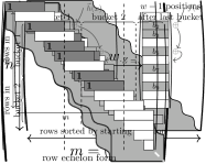
Figure 2: (a) Typical shape of the random matrix $A$ with rows ${(\vec{h}(x))_{x∈S}}$ sorted by starting positions. The shaded “ribbon” region contains random bits. Gaussian elimination never causes any fill-in outside of the ribbon.
(b) Shape of the linear system ${M}$ in row echelon form maintained using Boolean banding on the fly. In gray we visualize the insertion of a key $x$ where (i) $\smash{\vec{h}}(x)$ has its left-most $1$ in position $s(x)=2$, (ii) after xoring the second row of $M$ to $\smash{\vec{h}}(x)$, the left-most $1$ is in position $5$ and (iii) xoring the fifth row as well, the left-most $1$ is in position $6$. The resulting row fills the previously empty sixth row of $M$ and $f(x)⊕b₂⊕b₅$ is added as right hand side.

Ribbon solving. Our first contribution is a simple algorithm we could not resist to also call ribbon as in Rapid Incremental Boolean Banding ON the fly. It maintains a system of linear equations in row echelon form as shown in Figure 2 (b). It does so on-the-fly, i.e. while equations arrive one by one in arbitrary order. For each index $i$ of a column there may be at most one equation that has its leftmost one in column $i$. When an equation with row vector $a$ arrives and its slot is already taken by a row $a^{\prime}$, then ribbon performs the row operation $a\leftarrow a⊕a^{\prime}$, which eliminates the $1$ in position $i$, and continues with the modified row. An invariant is that rows have all their nonzeroes in a range of size $w$, which allows to process rows with a small number of bit-parallel word operations. This insertion process is incremental in that insertions do not modify existing rows. This improves performance and allows to cheaply roll back the most recent insertions which will be exploited below. It is a non-trivial insight that the order in which equations are added does not significantly affect the expected number of row operations.

When all rows processed we perform back-substitution to compute the solution matrix $Z$. At least for small $r$, interleaved representation of $Z$ works well, where blocks of size $w\times r$ of $Z$ are stored column-wise. A query for $x$ can then retrieve one bit of $f(x)$ at a time by applying a population count instruction to pieces of rows retrieved from at most two of these blocks. This is particularly advantageous for negative queries to AMQs (i.e. queries of elements not in the set), where only two bits need to be retrieved on average. More details are given in Section 6.

3.1 Standard Ribbon

When employing no further tricks, we obtain standard ribbon retrieval, which is essentially the same data structure as in [21] except with a different solver that is faster by noticeable constant factors. A problem is that $w$ has to become impractically large when $n$ is large and $\varepsilon$ is small. For example, in our experiments the smallest overhead we could achieve for $n=10^{6}$ and (already quite expensive) $w=128$ is around $3.3\,\%$ (for construction success rate $50\%$). To some degree this can be mitigated by sharding techniques [50], but in this paper we pursue a more ambitious route.

3.2 Bumped Ribbon Retrieval

Our main contribution is bumped ribbon retrieval (BuRR), which reduces the required ribbon width to a constant that only depends on the targeted space efficiency. BuRR is based on two ideas.

Bumping. The ribbon solving approach manages to insert most rows (representing most keys of $S$) even when $w$ is small. Thus, by eliminating those rows/keys that cause a linear dependency, we obtain a compact retrieval data structure for a large subset of $S$. The remaining keys are bumped, meaning they are handled by a fallback data structure which, by recursion, can be a BuRR data structure again. We show that only $𝒪(\frac{n\log w}{w})$ keys need to be bumped in expectation. Thus, after a constant number of layers (we use $4$), a less ambitious retrieval data structure can be used to handle the few remaining keys without bumping.

The main challenge is that we need additional metadata to encode which keys are bumped. The basic bumped retrieval approach is adopted from the updateable retrieval data structure filtered retrieval (FiRe) [44]. To shrink the input size by a moderate constant factor, FiRe needs a constant number of bits per key (around 4). This leads to very high space overhead for small $r$. A crucial observation for BuRR is that bumping can be done with coarser than per-key granularity. We will bump keys based on their starting position and say position $i$ is bumped to indicate that all keys with $s(x)=i$ are bumped. Bumping by position is sufficient because linear dependencies in $A$ are largely unrelated to the actual bit patterns $c(x)$ but mostly caused by fluctuations in the number of keys mapped to different parts of the matrix $A$. By selectively bumping ranges of positions in overloaded parts of the system, we can obtain a solvable system. Furthermore, our analysis shows that we can drastically limit the spectrum of possible bumping ranges, see below.

Overloading. Besides metadata, space overhead results from the $m-n+n_{b}$ excess slots of the table where $n_{b}$ is the number of bumped keys. Trying out possible values of $\varepsilon=\frac{m-n}{n}>0$ one sees that the overhead due to excess slots is always $\mathrm{\Omega}\!\left(1/w\right)$ and will thus dominate the overhead due to metadata. However, we show that by choosing $\varepsilon<0$ (of order $-ε=𝒪(\frac{\log w}{w})$), i.e., by overloading the table, we can almost completely eliminate excess table slots so that the minuscule amount of metadata becomes the dominant remaining overhead. There are many ways to decide and encode which keys are bumped. Here, we outline a simple variant that achieves very good performance in practice and is a generalization of the theoretically analyzed approach. We expand on the much larger design space of BuRR in Section 11.

Deciding what to bump. We subdivide the possible starting positions into buckets of width $b=\mathcal{O}\!\left(w^{2}/\log w\right)$ and allow to bump a single initial range of each bucket. The keys (or more precisely pairs of hashes and the value to be retrieved) are sorted according to the bucket addressed by the starting position $s(x)$. We use a fast in-place integer sorter for this purpose [2]. Then buckets are processed one after the other from left to right. Within a bucket, however, keys are inserted into the row echelon form from right to left. The reason for this is that insertions of the previous bucket may have “spilled over” causing additional load on the left of the bucket – an issue we wish to confront as late as possible. See also Figure 3.

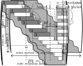
$\rightsquigarrow$      

Figure 3: Illustration of BuRR construction with $n=11$ keys, $m=2b+w-1=15$ table positions, ribbon width $w=4$ and bucket size $b=6$. Keys of the first bucket were successfully inserted into row echelon form with two insertions “overflowing” into the second bucket. Insertions of the second bucket’s rows will be attempted next, in the indicated order.

If all keys of a bucket can be successfully inserted, no keys of the bucket are bumped. Otherwise, suppose the first failed insertion for a bucket $[i,i+b)$ concerns a key where $s(x)=i+k$ is the $k$-th position of the bucket. We could decide to bump all keys $x^{\prime}$ of the bucket with $s(x^{\prime})≤i+k$, which would require storing the threshold $k$ using $𝒪(\log w)$ bits and which would yield an overhead of $𝒪(\log²(w)/w²)$ due to metadata. Instead, to reduce this overhead to $𝒪(\log(w)/w²)$, we only allow a constant number of threshold values. This means that we find the smallest threshold value $t$ with $t≥k$ representable by metadata and bump all keys $x^{\prime}$ with $s(x^{\prime})≤i+t$. This requires rolling back the insertions of keys $x^{\prime}$ with $s(x^{\prime})∈[k,t]$ by clearing the most recently populated rows from the row echelon form. One good compromise between space and speed stores 2 bits per bucket encoding the threshold values $\{0,\ell,u,b\}$, for suitable $\ell$ and $u$. The special case $\ell=u=\frac{3}{8}w$ is used in our analysis. Another slightly more compact variant “$1^{+}$-bit” stores one bit encoding threshold values from the set $\{0,t\}$, for a suitable $t$, and additionally stores a hash table of exceptions for thresholds $>t$.

Running times. With these ingredients we obtain Theorem 1.2 stated on page 1.2. It implies constant query time if $rw=\mathcal{O}\!\left(\log n\right)$ and linear construction time if $w\in\mathcal{O}\!\left(1\right)$. For wider ribbons, construction time is slightly superlinear. However, in practice this does not necessarily mean that BuRR is slower than other approaches with asymptotically better bounds as the factor $w$ involves operations with very high locality. An analysis in the external memory model reveals that BuRR construction is possible with a single scan of the input and integer sorting of $n$ objects of size $\mathcal{O}\!\left(\log n\right)$ bits, see Section 11.3.

3.3 Homogeneous Ribbon Filter

For the application of ribbon to AMQs, we can also compute a uniformly random solution of the homogeneous equation system $AZ=0$, i.e., we compute a retrieval data structure that will retrieve $0^{r}$ for all keys of $S$ but is unlikely to produce $0^{r}$ for other inputs. Since $AZ=0$ is always solvable, there is no need for bumping. The crux is that the false positive rate is no longer $2^{-r}$ but higher. In Section 9 we show that with table size $m=(1+\varepsilon)n$ and $ε=Ω(\frac{\max(r,\log w)}{w})$ the difference is negligible, thereby showing Theorem 1.3. Homogeneous ribbon AMQs are simpler and faster than BuRR but have higher space overhead. Our experiments indicate that together, BuRR and homogeneous ribbon AMQs cover a large part of the best tradeoffs for static AMQs.

3.4 Analysis outline

To get an intuition for the relevant linear systems, it is useful to consider two simplifications. First, assume that $\vec{h}(x)$ contains a block of $w$ uniformly random real numbers from $[0,1]$ rather than $w$ random bits. Secondly, assume that we sort the rows by starting position and use Gaussian elimination rather than ribbon to produce a row echelon form. In Figure 4 (a) we illustrate for such a matrix with $×$-marks where the pivots would be placed and in yellow the entries that are eliminated (with one row operation each); both with probability $1$, i.e. barring coincidences where a row operation eliminates more than one entry. The $×$-marks trace a diagonal through the matrix except that the green column and the red row are skipped because the end of the (gray) area of nonzeroes is reached. “Column failures” correspond to free variables and therefore unused space. “Row failures” correspond to linearly dependent equations and therefore failed insertions. This view remains largely intact when handling Boolean equations in arbitrary order except that the ribbon diagonal, which we introduce as an analogue to the trace of pivot positions, has a more abstract meaning and probabilistically suffers from row and column failures depending on its distance to the ribbon border.

(a)		(b)
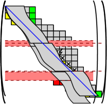
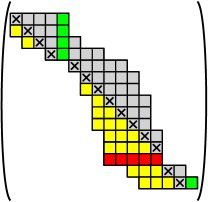
			$\longrightarrow$

Figure 4: (a) The simplified ribbon diagonal (made up of $×$-marks) passing through $A$.
(b) The idea of BuRR: When starting with an “overloaded” linear system and removing sets of rows strategically, we can often ensure that the ribbon diagonal does not collide with the ribbon border (except possibly in the beginning and the end).

The idea of standard ribbon is to give the gray ribbon area an expected slope of less than $1$ such that row failures are unlikely. BuRR, as illustrated in Figure 4 (b) largely avoids both failure types by using a slope bigger than $1$ but removing ranges of rows in strategic positions. Homogeneous ribbon filters, despite being the simplest approach, have the most subtle analysis as both failure types are allowed to occur. While row failures cannot cause outright construction failure, they are linked to a compromised false positive rate in a non-trivial way. Our proofs involve mostly simple techniques as would be used in the analysis of linear probing, which is unsurprising given that [21] has already established a connection to Robin Hood hashing. We also profit from queuing theory via results we import from [21].

3.5 Further results

We have several further results around variants of BuRR that we summarize here.

Perhaps most interesting is bump-once ribbon retrieval (Bu¹RR), which improves the worst-case query time by guaranteeing that each key can be retrieved from one out of two layers – its primary layer or the next one. The primary layer of the keys is now distributed over all layers (except for the last). When building a layer, the keys bumped from the previous layer are inserted into the row echelon form first. The layer sizes have to be chosen in such a way that no bumping is needed for these keys with high probability. Only then are the keys with the current layer as their primary layer inserted – now allowing bumping. See Section 11.4 for details.

For building large retrieval data structures, parallel construction is important. Doing this directly is difficult for ribbon retrieval since there is no efficient way to parallelize back-substitutions. However, we can partition the equation system into parts that can be solved independently by bumping $w$ consecutive positions. Note that this can be done transparently to the query algorithm by using the bumping mechanism that is present anyway. See Section 11.3 for details.

For large $r$, we accelerate queries by working with sparse bit patterns that set only a small fraction of the $w$ bits in the window used for BuRR. In some sense, we are covering here the middle ground between ribbon and spatial coupling [51]. Experiments indicate that setting 8 out of 64 bits indeed speeds up queries for $r\in\{8,16\}$ at the price of increased (but still small) overhead. Analysis and further exploration of this middle ground may be an interesting area for future work.

4 Summary of Experimental Findings

We performed extensive experiments to evaluate our ribbon-based data structures and competitors. We summarize our findings here with details provided in Section 12. Two preliminary remarks are in order: Firstly, since every retrieval data structure can be used as a filter but not vice versa, our experiments are for filters, which admits a larger number of competitors. Secondly, to reduce complexity (for now), our speed ranking considers the sum of construction time per key and three query times.

Ribbon yields the fastest static AMQs for overhead $\bm{<44\%}$.

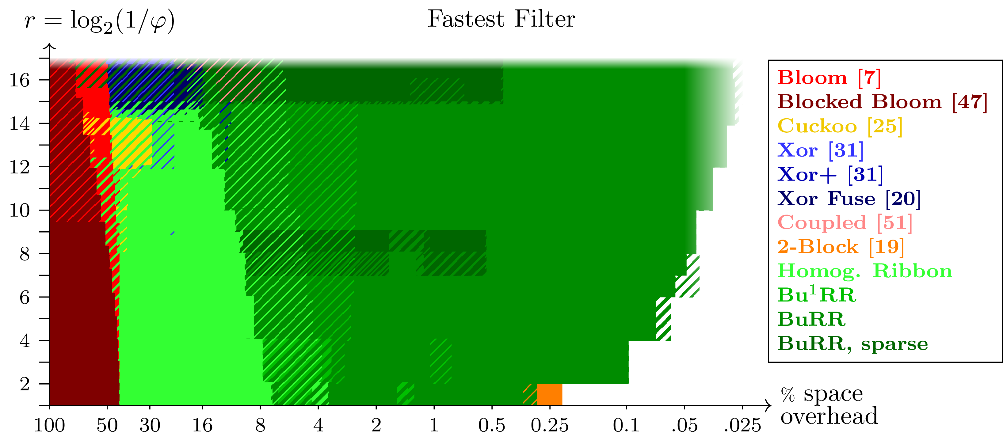
Figure 5: Fastest AMQ category for different choices of overhead and false-positive rate $ϕ=2^{-r}$. Shaded regions indicates a dependency on the input type. Ranking metric: construction time per key plus time for three queries, of which one is positive, one negative, and one mixed (50 % chance of either).

Consider Figure 1 on page 1, where we show the tradeoff between space overhead and computation cost for a range of AMQs for false positive rate $ϕ\approx 2^{-8}$ (i.e., $r=8$ for BuRR) and large inputs. In the parallel workload on the right all cores access many AMQs randomly.

Only three AMQs have Pareto-optimal configurations for this case: BuRR for space overhead below 5 % (actually achieving between 1.4 % and 0.2 % for a narrow time range of 830–890 ns), homogeneous ribbon for space overhead below 44 % (actually achieving between 20 % and 10 % for a narrow time range 580–660 ns), and blocked Bloom filters [47] with time around 400 ns at the price of space overhead of around 50 %. All other tried AMQs are dominated by homogeneous ribbon and BuRR. Somewhat surprisingly, this even includes plain Bloom filters [7] which are slow because they incur several cache faults for each insertion and positive query. Since plain Bloom filters are extensively used in practice (often in cases where a static interface suffices), we conclude that homogeneous ribbon and BuRR are fast enough for a wide range of applications, opening the way for substantial space savings in those settings. BuRR is at least twice as fast as all tried retrieval data structures. The filter data structures that support counting and deletion (Cuckoo filters [25] and the related Morton filters [11] as well as the quotient filters QF [40] and CQF [5]) are slower than the best static AMQs.

The situation changes slightly when going to a sequential workload with large inputs as shown on the left of Figure 1.Blocked Bloom and BuRR are still the best filters for large and small overhead, respectively. But now homogeneous ribbon and (variants of) the hypergraph peeling based Xor filters [31, 20] share the middle-ground of the Pareto curve between them. Also, plain Bloom filters are almost dominated by Xor filters with half the overhead. The reason is that modern CPUs can handle several main memory accesses in parallel. This is very helpful for Bloom and Xor, whose queries do little else than computing the logical (x)or of a small number of randomly chosen memory cells. Nevertheless, the faster variants of BuRR are only moderately slower than Bloom and Xor filters while having at least an order of magnitude smaller overheads.

Further Results. Other claims supported by our data are:

• • Good ribbon widths are $w=32$ and $w=64$. Ribbon widths as small as $w=16$ can achieve small overhead but at least on 64-bit processors, $w\in\{32,64\}$ seems most sensible. The case $w=32$ is only 15–20 % faster than $w=64$ while the latter has about four times less overhead. Thus the case $w=64$ seems the most favorable one. This confirms that the linear dependence of the construction time on $w$ is to some extent hidden behind the cache faults which are similar for both values of $w$ (this is in line with our analysis in the external memory model). • Bu¹RR is slower than BuRR by about 20 %, which may be a reasonable price for better worst-case query time in some real-time applications. • The $\bm{1^{+}}$-bit variant of BuRR is smaller but slower than the variant with 2-bit metadata per bucket, as expected, though not by a large margin. • Smaller inputs and smaller $\bm{r}$ change little. For inputs that fit into cache, the Pareto curve is still dominated by blocked Bloom, homogeneous ribbon, and BuRR, but the performance penalty for achieving low overhead increases. For $r=1$ we have data for additional competitors. GOV [29], which relies on structured Gaussian elimination, is several times slower than BuRR and exhibits an unfavorable time–overhead tradeoff. 2-block [19] uses two small dense blocks of nonzeroes and can achieve very small overhead at the cost of prohibitively expensive construction. • For large $\bm{r}$, Xor filters and Cuckoo filters come into play. Figure 5 shows the fastest AMQ depending on overhead and false positive rate $ϕ=2^{-r}$ up to $r=16$. While blocked Bloom, homogeneous ribbon, and BuRR cover most of the area, they lose ground for large $r$ because their running time depends on $r$. Here Xor filters and Cuckoo filters make an appearance. • Bloom filters and Ribbon filters are fast for negative queries where, on average, only two bits need to be retrieved to prove that a key is not in the set. This improves the relative standing of plain Bloom filters on large and parallel workloads with mostly negative queries. • Xor filters [31] and Coupled [51] have fast queries since they can exploit parallelism in memory accesses. They suffer, however, from slow construction on large sequential inputs due to poor locality, and exhibit poor query performance when accessed from many threads in parallel. For small $n$, large $r$, and overhead between 8 % and 20 %, Coupled becomes the fastest AMQ.

5 Related Results and Techniques

We now take the time to review some related work on retrieval including all approaches listed in Table 1.

Related Problems. An important application of retrieval besides AMQs is encoding perfect hash functions (PHF), i.e. an injective function $p:S\textrightarrow[(1+ε)|S|]$ for given $S⊆\mathcal{U}$. Objectives for $p$ are compact encoding, fast evaluation and small $ε$. Consider a result from cuckoo hashing [26, 27, 37], namely that given four hash functions $h₁,h₂,h₃,h₄:S\textrightarrow[1.024|S|]$ there exists, with high probability, a choice function $f:S\textrightarrow[4]$ such that $x↦h_{f(x)}(x)$ is injective. A $2$-bit retrieval data structure for $f$ therefore gives rise to a perfect hash function [10], see also [13]. Retrieval data structures can also be used to directly store compact names of objects, e.g., in column-oriented databases [44]. This takes more space than perfect hashing but allows to encode the ordering of the keys into the names.

In retrieval for AMQs and PHFs the stored values $f(x)∈\{0,1\}^{r}$ are uniformly random. However, some authors consider applications where $f(x)$ has a skewed distribution and the overhead of the retrieval data structure is measured with respect to the $0$-th order empirical entropy of $f$ [32, 4, 29]. Note that once we can do 1-bit retrieval with low overhead, we can use that to store data with prefix-free variable-bit-length encoding (e.g. Huffman or Golomb codes). We can store the $k$-th bit of $f(x)$ as data to be retrieved for the input tuple $(x,k)$. This can be further improved by storing $R$ 1-bit retrieval data structures where $R=\max_{x∈S}|f(x)|$ [32, 4, 29]. By interleaving these data structures, one can make queries almost as fast as in the case of fixed $r$.

More Linear Algebra based approaches. It has long been known that some matrices with random entries are likely to have full rank, even when sparse [14] and density thresholds for random $k$-XORSAT formulas to be solvable – either at all [24, 16] or with a linear time peeling algorithm [42, 33] – have been determined.

Building on such knowledge, a solution to the retrieval problem was identified by Botelho, Pagh and Ziviani [9, 8, 10] in the context of perfect hashing. In our terminology, their rows $\vec{h}(x)$ contain $3$ random $1$-entries per key which makes $AZ=\bm{b}$ solvable with peeling, provided $m>1.22n$.

Several works develop the idea from [10]. In [28, 29] only $m>1.089n$ is needed in principle (or $m>1.0238n$ for $|\vec{h}(x)|=4$) but a Gaussian solver has to be used. More recently in the spatial coupling approach [51] $\smash{\vec{h}}(x)$ has $k$ random $1$-entries within a small window, achieving space overhead $\approx e^{-k}$ while still allowing a peeling solver. With some squinting, a class of linear erasure correcting codes from [38] can be interpreted as a retrieval data structure of a similar vein, where $|\vec{h}(x)|∈\{5,…,k\}$ is random with expectation $\mathcal{O}(\log k)$.

Two recent approaches also based on sparse matrix solving are [19, 21] where $\vec{h}(x)$ contains two blocks or one block of random bits. Our ribbon approach builds on the latter.

We end this section with a discussion of seemingly promising techniques and give reasons why we choose not to use them in this paper. Some more details on methods used in the experiments are also discussed in Section 12.

Shards. A widely used technique in hashing-based data structures is to use a splitting hash function to first divide the input set into many much smaller sets (shards, buckets, chunks, bins,…) that can then be handled separately [29, 3, 19, 21, 1, 46]. This incurs only linear time overhead during preprocessing and constant time overhead during a query, and allows to limit the impact of superlinear cost of further processing to the size of the shard. Even to ribbon, this could be used in multiple ways. For example, by statically splitting the table into pieces of size $n^{ε}$ for standard ribbon, one can achieve space overhead $ε+\mathcal{O}\!\left(n^{-ε}\right)$, preprocessing time $\mathcal{O}\!\left(n/ε\right)$, and query time $\mathcal{O}\!\left(r\right)$ [21]. This is, however, underwhelming on reflection. Before arriving at the current form of BuRR, we designed several variants based on sharding but never achieved better overhead than $\mathrm{\Omega}\!\left(1/w\right)$. The current overhead of $\mathcal{O}\!\left(\log w/w^{2}\right)$ comes from using the splitting technique in a “soft” way – keys are assigned to buckets for the purpose of defining bumping information but the ribbon solver may implicitly allocate them to subsequent buckets.

Table lookup. The first asymptotically efficient succinct retrieval data structure we are aware of [46] uses two levels of sharding to obtain very small shards of size $\mathcal{O}\!\left(\sqrt{\log n}\right)$ with small asymptotic overhead. It then uses dense random matrices per shard to obtain per-shard retrieval data structures. This can be done in constant time per shard by tabulating the solutions of all possible matrices. This leads to a multiplicative overhead of $\mathcal{O}\!\left(\log\log n/\sqrt{\log n}\right)$. Belazzougui and Venturini [4] use slightly larger shards of size $\mathcal{O}\!\left((1+\log\log(n)/r)\log\log(n)/\log n\right)$. Using carefully designed random lookup tables they show that linear construction time, constant lookup time, and overhead $\mathcal{O}\!\left((\log\log n)^{2}/\log n\right)$ is possible. We discussed on page 1 why we suspect large overhead for [46] and [4] in practice.

In general, lookup tables are often problematic for compressed data structures in practice – they cause additional space overhead and cache faults. Even if the table is small and fits into cache, this may yield efficient benchmarks but can still cause cache faults in practical workloads where the data structure is only a small part in a large software system with a large working set.

Cascaded bumping. Hash tables consisting of multiple shrinking levels are also used in multilevel adaptive hashing [12] and filter hashing [26]. While similar to BuRR in this sense, they do not maintain bumping information. This is fine for storing key-value pairs because all levels can be searched for a requested key. But it is unclear how the idea would work in the context of retrieval, i.e. without storing keys.

6 Ribbon Insertions

In this section we enhance the SGAUSS construction for retrieval from [21] with a new solver called Rapid Incremental Boolean Banding ON the fly (Ribbon), which is the basis of all ribbon variants considered later.

The SGAUSS construction. For a parameter $w\in{\rm Nature}$ that we call the ribbon width, the vector $\smash{\vec{h}}(x)∈\{0,1\}^{m}$ is given by a random starting position $s(x)∈[m-w-1]$ and a random coefficient vector $c(x)∈\{0,1\}^{w}$ as $\smash{\vec{h}}(x)=0^{s(x)-1}c(x)0^{m-s(x)-w+1}$. Note that even though $m$-bit vectors like $\smash{\vec{h}}(x)$ are used to simplify mathematical discussion, such vectors can be represented using $\log(m)+w$ bits. The matrix $A$ with rows $(\smash{\vec{h}}(x))_{x∈S}$ sorted by $s(x)$ has all of its $1$-entries in a “ribbon” of width $w$ that randomly passes through the matrix from the top left to the bottom right, as in Figure 2 (a). The authors show:

Theorem 6.1 ([21, Thm 2]).

For any constant $0<ε<\frac{1}{2}$ and $\frac{n}{m}=1-ε$ there is a suitable choice for $w=Θ(\smash{\frac{\log n}{ε}})$ such that with high probability the linear system $(\smash{\vec{h}}(x)·Z=f(x))_{x∈S}$ is solvable for any $r∈ℕ$ and any $f:S\textrightarrow\{0,1\}^{r}$. Moreover, after sorting $(\smash{\vec{h}}(x))_{x∈S}$ by $s(x)$, Gaussian elimination can compute a solution $Z$ in expected time $\mathcal{O}(n/ε²)$.

Boolean banding on the fly. For ribbon retrieval we use the same hash function $\smash{\vec{h}}$ as in SGAUSS except that we force coefficient vectors $c(x)$ to start with $1$, which slightly improves presentation and prevents construction failures caused by single keys with $c(x)=0^{w}$. The main difference lies in how we solve the linear system. The insertion phase maintains a system $M$ of linear equations in row echelon form using on-the-fly Gaussian elimination [6]. This system is of the form shown in Figure 2 (b) and has $m$ rows that we also call slots. The $i$-th slot contains a $w$-bit vector $c_{i}∈\{0,1\}^{w}$ and $b_{i}∈\{0,1\}^{r}$. Logically, the $i$-th slot is either empty ($c_{i}=0^{w}$) or specifies a linear equation $c_{i}·Z_{[i,i+w)}=b_{i}$ where $c_{i}$ starts with a $1$. With $Z_{[i,i+w)}∈\{0,1\}^{w×r}$ we refer to rows $i,…,i+w-1$ of $Z∈\{0,1\}^{w×r}$. We ensure $c_{i}·Z_{[i,i+w)}$ is well-defined even when $i+w-1>m$ with the invariant that $c_{i}$ never selects “out of bounds” rows of $Z$.

We consider the equations $\smash{\vec{h}}(x)·Z=f(x)$ for $x∈S$ one by one, in arbitrary order, and try to integrate each into $M$ using Algorithm 1, which we explain now.

1 $(i,c,b)\textleftarrow(s(x),c(x),f(x))$

2 loop  

3       if $M.c[i]=0$ then // slot $i$ of $M$ is empty

4             $(M.c[i],M.b[i])\textleftarrow(c,b)$

5             return success

6      $(c,b)\textleftarrow(c⊕M.c[i],b⊕M.b[i])$

7       if $c=0$ then

8             if $b=0$ then  return redundant

9             else  return failure

10            

11      $j\textleftarrow\mathrm{findFirstSet}(c)$ // a.k.a. BitScanForward

12       $i\textleftarrow i+j$

13       $c\textleftarrow c>>j$ // logical shift last toward first

14      

Algorithm 1 Adding a key’s equation to the linear system $M$.

A key’s equation may be modified several times before it can be added to $M$, but a loop invariant is that its form is

$$c·Z_{[i,i+w)}=b\text{ for some $i∈[m]$, $c∈1∘\{0,1\}^{w-1}$, $b∈\{0,1\}^{r}$.}$$ (1)

The initial equation $\smash{\vec{h}}(x)·Z=f(x)$ of key $x∈S$ has this form with $i=s(x)$, $c=c(x)$ and $b=f(x)$.

•[Case 1:] In the simplest case, slot $i$ of $M$ is empty and we can store Equation 1 in it. •[Case 2:] Otherwise slot $i$ of $M$ is occupied by an equation $c_{i}·Z_{[i,i+w)}=b_{i}$. We perform a row operation to obtain the new equation

$$c^{\prime}·Z_{[i,i+w)}=b^{\prime}\text{ with $c^{\prime}=c⊕c_{i}$ and $b^{\prime}=b⊕b_{i}$,}$$ (2)

which, in the presence of the equation in slot $i$ of $M$, puts the same constraint on $Z$ as Equation 1. Both $c$ and $c_{i}$ start with $1$, so $c^{\prime}$ starts with $0$. We consider the following sub-cases.

•[Case 2.1:] $c^{\prime}=0^{w}$ and $b^{\prime}=0^{r}$. The equation is void and can be ignored. This happens when the original equation of $x$ is implied by equations previously added to $M$. •[Case 2.2:] $c^{\prime}=0^{w}$ and $b^{\prime}≠0^{r}$. The equation is unsatisfiable. This happens when the key’s original equation is inconsistent with equations previously added to $M$. •[Case 2.3:] $c^{\prime}$ starts with $j>0$ zeroes followed by a $1$. Then Equation 2 can be rewritten as $c^{\prime\prime}·Z_{[i^{\prime},i^{\prime}+w)}=b^{\prime}$ where $i^{\prime}=i+j$ and $c^{\prime\prime}$ is obtained from $c^{\prime}$ by discarding the $j$ leading zeroes of $c$ and appending $j$ trailing zeroes.

Termination is guaranteed since $i$ increases with each loop iteration.

“On-the-fly” and “incremental.” The insertion phase of Ribbon is on-the-fly [6], i.e. maintains a row echelon form as keys arrive. This allows us to determine the longest prefix $(x₁,…,x_{n})$ of a sequence $S=(x₁,x₂,x₃,…)$ of keys for which construction succeeds: Simply insert keys until the first failure. We say the insertion phase is incremental since an insertion may lead to a new row in $M$ but does not modify existing rows. This allows us to easily undo the most recent successful insertions by clearing the slots of $M$ that were filled last. These properties are not shared by SGAUSS and will be exploited by BuRR in Section 10.

Efficiency. Running times of SGAUSS and Ribbon are tied in $\mathcal{O}$-notation. However, Ribbon improves upon SGAUSS in constant factors for the following reasons:

• • Ribbon need not pre-sort the keys by $s(x)$. • During construction, SGAUSS explicitly maintains for each row the index of the left-most $1$. Ribbon represents these implicitly, saving significant amounts memory. • SGAUSS performs some number $D$ of elimination steps, which, depending on some bit, turn out to be xor-operations or no-ops. Ribbon on the other hand performs roughly $D/2$ bit shifts and $D/2$ (unconditional) xor operations. Though the details are complicated, intuition on branching complexity seems to favor Ribbon.

7 Analysis of Ribbon Insertions

Given a set $S$ of $n$ keys we wish to analyze the process of inserting these keys into the system $M$ using Algorithm 1. In particular, we are interested in the number of successful and failed insertions, the set of occupied slots in $M$ and the total running time. Recall that $A∈\{0,1\}^{n×m}$ contains the rows $\smash{\vec{h}}(x)$ for $x∈S$ sorted by $s(x)$, see Figure 2 (a). Our analysis considers the ribbon diagonal, which is a line passing through $A$. We begin with an instructive simplification.

7.1 A Warm Up: The Simplified Ribbon Diagonal

We make the following two assumptions:

(M1)

Keys are inserted in the order they appear in $A$ (sorted by $s(x)$). This ensures that the insertion of each key $x∈S$ fails or succeeds within the first $w$ steps because no $1$-entries can exist in $M$ beyond column $s(x)+w-1$.

(M2)

Inserting $x∈S$ fills the first free slot $i∈[s(x),s(x)+w-1]$ unless all of these slots are occupied, in which case the insertion fails. This ignores the role of $c(x)$.

Figure 4 visualizes the process with an $×$ in position $(j,i)$ if the insertion of the $j$-th key fills slot $i$ of $M$. These points approximately trace a diagonal line from top left to bottom right and we call it the simplified ribbon diagonal $d_{\mathrm{simp}}$. We make the following observations:

(O1)

If $d_{\mathrm{simp}}$ were to cross the bottom border of the ribbon, it skips a column (shown in green). Column $i$ is skipped if and only if slot $i$ of $M$ remains empty.

(O2)

If $d$ were to cross the right border of the ribbon, it skips a row (shown in red). Row $j$ is skipped if and only if the $j$-th key is not inserted successfully.

(O3)

The area enclosed between $d$ and the left border of the ribbon (shown in yellow) is an upper bound on the number of row operations performed during successful insertions.

7.2 The Ribbon Diagonal

A formal analysis can salvage much of the intuition from the simplified model. First, we show that (M1), though not (M2), can be made without loss of generality. For an adjusted definition of the ribbon diagonal, we then prove probabilistic versions of (O1), (O2) and (O3). The following notation will be useful.

• • $S_{i}=\{x∈S\mid s(x)≤i\}$ and $s_{i}=|S_{i}|$, for $i∈[m]$. • $S^{\prime}⊆S$ is the set of keys not inserted successfully. Moreover, $S^{\prime}_{i}=S_{i}∩S^{\prime}$ and $s_{i}^{\prime}=|S^{\prime}_{i}|$. • $r_{i}$, for $i∈[m]$, is the rank of the first $i$ columns of $A$. • $P_{M}$ is the set of slots of $M$ that end up being filled.

On (M1): The order of keys is irrelevant.

Since $M$ arises from $A$ by row operations, which do not affect ranks of sets of columns, we conclude that $r_{i}$ is the rank of the first $i$ columns of $M$, regardless of the order in which keys are handled. From the form of $M$ (see Figure 2 (b)) it is clear that $i∈P_{M}⇔r_{i}=r_{i-1}+1$. Therefore, the set $P_{M}$ and thus the number $n-|P_{M}|=|S^{\prime}|$ of failed insertions is also invariant.

Assuming all insertions are successful, the number of row operations performed for key $x$ is at most the distance of $s(x)$ to the slot $i(x)∈P_{M}$ that is filled. An invariant upper bound $Δ$ on the number of row operations, which are the dominating contribution to construction time, is then

$$Δ:=\sum_{x∈S}(i(x)-s(x))=\sum_{i∈P_{M}}i-\sum_{x∈S}s(x).$$ (3)

Except for the time related to failed insertions, which we have to bound separately, we can derive everything we want from $S$ and the invariants $P_{M}$, $|S^{\prime}|$. We can therefore assume (M1).

Definition and properties of $d$.

Given (M1), we formally define the ribbon diagonal $d$ as the following set of matrix positions in $A$.

$$d=\{(d_{i},i)\mid i∈[m]\}\text{ where }d_{i}=r_{i}+s^{\prime}_{i-w+1}.$$

It is useful to imagine the “default case” to be $r_{i}=r_{i-1}+1$ and $s^{\prime}_{i}=s^{\prime}_{i-1}$. We then have $d_{i}=d_{i-1}+1$ and the ribbon diagonal indeed moves diagonally down and to the right. An empty slot $i∉P_{M}$ correspond to a right-shift (due to $r_{i}=r_{i-1}$) and a failed insertion of a key with $s(x)=i-w+1$ correspond to a down-shift (due to $s^{\prime}_{i-w+1}>s^{\prime}_{i-w}$).

Let us first check that $d$ is actually within the ribbon. More precisely:

Lemma 7.1.

For any $i∈[m]$, $d_{i}$ is not below the bottom ribbon border $s_{i}$ and at most one position above the top ribbon border $s_{i-w}+1$.

Proof 7.2.

The first claim holds because

$$d_{i}=r_{i}+s^{\prime}_{i-w+1}≤r_{i}+s^{\prime}_{i}=|P_{M}∩[1,i]|+s^{\prime}_{i}≤s_{i}$$

where the last step uses that each key in $S_{i}$ can fail to be inserted or fill a slot in $M$, but not both. The latter is true because

$$d_{i}=|P_{M}∩[1,i]|+s^{\prime}_{i-w+1}≥(s_{i-w+1}-s^{\prime}_{i-w+1})+s^{\prime}_{i-w+1}=s_{i-w+1}≥s_{i-w}.$$

where the first “$≥$” uses that the first $s_{i-w+1}$ rows cause $s_{i-w+1}-s^{\prime}_{i-w+1}$ slots with index at most $i$ to be filled.

The first part of Lemma 7.1 ensures that the height $h_{i}:=s_{i}-d_{i}$ of the ribbon diagonal above the bottom ribbon border is non-negative. It plays a central role in the precise versions of (O1) to (O3) we prove next. The main adjustment we have to make is that $d$ is probabilistically repelled when close to the ribbon border, while $d_{\mathrm{simp}}$ only responds to outright collisions.

Lemma 7.3 (Precise version of (O1)).

We have $\Pr[i∉P_{M}\mid h_{i-1}=k]≤2^{-k}$ for any $k∈ℕ₀$.

Proof 7.4.

A useful alternative way to think about Algorithm 1 uses language from linear probing: A key $x$ probes slots $s(x),s(x)+1,…,s(x)+w-1$ one by one. When probing an empty slot, $x$ is inserted into that slot with probability $\frac{1}{2}$, otherwise it keeps probing. Now consider slot $i$. Of the $s_{i-1}$ keys with starting position at most $i-1$, precisely $r_{i-1}$ are successfully inserted to slots in $[1,i-1]$ and $s^{\prime}_{i-w}$ insertions fail without probing slot $i$. Therefore $s_{i-1}-s^{\prime}_{i-w}-r_{i-1}=s_{i-1}-d_{i-1}=h_{i-1}$ keys probe slot $i$. So conditioned on $h_{i-1}=k$, slot $i$ remains empty with probability at most $2^{-k}$.

Lemma 7.5 (Precise version of (O2)).

Let $x$ be a key with $s(x)=i$.

1. • Let $i^{\prime}∈[i,i+w]$ be the column of $A$ where the ribbon diagonal passes the row of $x$. Assume $i^{\prime}-i=w-k$, i.e. $i^{\prime}$ is $k$ positions left of the right ribbon border. Conditioned on this, $\Pr[x∈S^{\prime}]≤2^{-k}$. • A simple variant of this claim is: If $h_{i}≤w-k$ for some $k∈ℕ$ then $\Pr[x∈S^{\prime}]≤2^{-k}$.

Proof 7.6.

1. • Let $i=s(x)$. We may assume that $x$ is the last key with starting position $i$ as this can only increase $\Pr[x∈S^{\prime}]$. This means $x$ corresponds to row $s_{i}$ and hence $d_{i^{\prime}}≥s_{i}$. Of the $s_{i}-1$ keys that are handled before $x$, exactly $r_{i-1}$ are inserted before slot $i$ and at least $s_{i-1}^{\prime}$ were not inserted successfully. The number of slots in $[i,m]$ that are occupied when $x$ is handled is therefore at most

   $$s_{i}-1-r_{i-1}-s_{i-1}^{\prime}≤d_{i^{\prime}}-1-r_{i-1}-s_{i-1}^{\prime}=r_{i^{\prime}}+s_{i^{\prime}-w+1}-1-r_{i-1}-s_{i-1}^{\prime}$$

   $$≤r_{i^{\prime}}-r_{i-1}-1≤i^{\prime}-i=w-k.$$

   This means at least $k$ slots within $[i,i+w-1]$ are empty. The probability that $x$ cannot be inserted despite probing these $k$ slots is $2^{-k}$. • The assumption gives an alternative way to derive the same intermediate step:

   $$s_{i}-1-r_{i-1}-s_{i-1}^{\prime}≤s_{i}-r_{i}-s_{i-w+1}^{\prime}=s_{i}-d_{i}=h_{i}≤w-k.$$

Lemma 7.7 (Precise version of (O3)).

Let $\mathrm{op}₊$ be the number of row operations performed during successful insertions. We have $\mathrm{op}₊≤n(w-1)$ (trivially) as well as $\mathrm{op}₊≤\sum_{i∈[m]}h_{i}$.

Proof 7.8.

First assume that all insertions succeed and consider Equation 3. Since $i(x)-s(x)≤w-1$ holds for all $x∈S$ the trivial bound $\mathrm{op}₊≤Δ≤n(w-1)$ follows. Now consider the right hand side of Equation 3. The sum $\sum_{x∈S}(s(x)-1)$ can be interpreted as the area in $A$ (i.e. the number of matrix positions) left of the ribbon. Moreover we have

$$\sum_{i∈P_{M}}(i-1)=\sum_{i∈[m]}|P_{M}∩[i+1,m]|=\sum_{i∈[m]}n-r_{i}=\sum_{i∈[m]}n-d_{i}.$$

which is the area below the ribbon diagonal. This makes $Δ$ the area enclosed between the ribbon diagonal and the lower ribbon border. A column-wise computation of this area yields $\mathrm{op}₊≤Δ=\sum_{i∈[m]}h_{i}$ as desired.

Contrary to our initial assumption, there may be keys that fail to be inserted. But our bounds remain valid in the presence of such keys: The number $\mathrm{op}₊$ only counts operations made for successfully inserted keys and hence does not change. Our bounds $n(w-1)$ and $\sum_{i∈[m]}h_{i}$ are easily seen to increase by $w-1$ and $w$, respectively, for each additional “failing” key we take into account.

7.3 Chernoff Bounds

The following lemma will play a role in Sections 9 and 10.

Lemma 7.9.

Let $(X_{j})_{j∈[N]}$ be i.i.d. indicator random variables, $X:=\sum_{j∈[N]}X_{j}$ and $μ:=\mathbb{E}X$.

1. • For $δ∈[0,1]$ we have $\Pr[|X-μ|≥δμ]≤2\exp(-δ²μ/3)$. • There exists $C>0$ such that for any $w∈ℕ$ and $μ≤\frac{2w²}{C\log w}$ we have $\Pr[|X-μ|≥\tfrac{w}{8}]=\mathcal{O}(w^{-5})$.

Proof 7.10.

1. • This combines standard Chernoff bounds on the probability of $\{X≥(1+δ)μ\}$ and $\{X≤(1-δ)μ\}$ as found for instance in [41, Chapter 4]. • We set $δ=\frac{w}{8μ}$ and apply (a). This gives

   $$\Pr[|X-μ|≥\tfrac{w}{8}]≤2\exp(-δ²μ/3)=2\exp(-\tfrac{w²}{192μ})≤2\exp(-\tfrac{C\log w}{384})=2w^{-C/384}.$$

   Choosing $C=1920$ achieves the desired bound.

8 Analysis of Standard Ribbon Retrieval

By standard ribbon we mean the original design from [21], except that we use our improved solver. We sketch an implementation in Algorithm 2 and recall the broad strokes of the analysis from [21] which will help us to analyze homogeneous ribbon filters in Section 9.

Given $n∈ℕ$ keys we allocate a system $M$ of size $m=n/(1-ε)+w-1$ and try to insert all keys using Algorithm 1. If any insertion fails, the entire construction is restarted with new hash functions. Otherwise, we obtain a solution $Z$ to $M$ in the back substitution phase. The rows of $Z$ are obtained from bottom to top. If slot $i$ of $M$ contains an equation then this equation uniquely determines row $i$ of $Z$ in terms of later rows of $Z$. If slot $i$ of $M$ is empty, then row $i$ of $Z$ can be initialized arbitrarily.

Input: $f:S\textrightarrow\{0,1\}^{r}$ for some $S⊆\mathcal{U}$ of size $n$.

Parameters: $w∈ℕ$, $ε>0$.

1 $m\textleftarrow n/(1-ε)+w-1$; allocate system $M$ of size $m$

2 pick hash functions $s:\mathcal{U}\textrightarrow[m-w+1],\ c:\mathcal{U}\textrightarrow\{0,1\}^{w}$

3 for $x∈S$ do

4       $\mathrm{ret}\textleftarrow\mathrm{insert}(x)$ // using Algorithm 1

5       if $\mathrm{ret}=\text{failure}$ then

6             restart

7            

8      

9$Z\textleftarrow 0^{m×r}$

10 for $i=m$ down to $1$ do

11       $Z_{i}\textleftarrow M.c[i]·Z_{i..i+w-1}$ // back substitution

12      

13return $(s,c,Z)$

Algorithm 2 The construction algorithm of standard ribbon.

The expected “slope” of the ribbon is $1-ε$, giving us reason to hope that the ribbon diagonal will stick to the left ribbon border making failures unlikely.

Lemma 8.1.

The heights $h_{i}:=s_{i}-d_{i}$ for $i∈[m]$ satisfy:

1. • $𝔼[h_{i}]≤𝒪(1/ε)$ • $∀k∈ℕ:\Pr[h_{i}>k]=\exp(-Ω(εk))$.

Proof 8.2 (Proof idea from [21].).

By definition of $h_{i}$, $d_{i}$ and $r_{i}$ we have

$$h_{i}-h_{i-1} =(s_{i}-s_{i-1})-(r_{i}-r_{i-1})-(s^{\prime}_{i-w+1}-s^{\prime}_{i-w})$$

$$≤(s_{i}-s_{i-1})-(r_{i}-r_{i-1})=(s_{i}-s_{i-1})-𝟙_{i∈P_{M}}.$$

The number $s_{i}-s_{i-1}$ of keys with starting position $i$ has distribution $\mathrm{Bin}(n,\frac{1}{m-w+1})$ which is approximately $\mathrm{Po}(1-ε)$. By Lemma 7.3 we have $\Pr[i∉P_{M}]≤2^{-h_{i-1}}$. Roughly speaking this means that $\Pr[𝟙_{i∈P_{M}}≠1]$ is negligible as soon as $h_{i-1}$ rises to a value large enough to threaten the upper bounds we intend to prove. A coupling argument then allows us to upper bound $h_{i}$ in terms of a so-called M/D/1 queue. In every time step $\mathrm{Po}(1-ε)$ customers arrive and $1$ customer can be serviced. The stated bounds on (a) expectation and (b) tails of $h_{i}$ stem from the literature on such queues.

We remark that the term $s^{\prime}_{i-w+1}-s^{\prime}_{i-w}$ that we ignored relates to failed insertions. It translates to customers abandoning the queue after waiting for $w$ time steps without being serviced.

By choosing $w=Ω(\frac{\log n}{ε})$ it follows from Lemma 8.1 (b) that $h_{i}≤w/2$ for all $i∈[m]$ whp. Lemma 7.5 (b) then ensures that all keys can be inserted successfully whp. Combining Lemma 7.7 with Lemma 8.1 (a) shows that the expected number of row operations during construction is $\mathcal{O}(n/ε)$. This proves Theorem 1.1.

9 Analysis of Homogeneous Ribbon Filters

In this section we give a precise description and analysis of homogeneous ribbon filters, which are even simpler than filters based on standard ribbon but unsuitable for retrieval.

Recall the approach for constructing a filter by picking hash functions $\smash{\vec{h}}:\mathcal{U}\textrightarrow\{0,1\}^{m}$, $f:\mathcal{U}\textrightarrow\{0,1\}^{r}$ and finding $Z∈\{0,1\}^{m×r}$ such that all $x∈S$ satisfy $\smash{\vec{h}}(x)·Z=f(x)$, while most $x∈\mathcal{U}\setminus S$ do not. We now dispose of the fingerprint function $f$, effectively setting $f(x)=0$ for all $x∈\mathcal{U}$. A filter is then given by a solution $Z$ to the homogeneous system $(\smash{\vec{h}}(x)·Z=0^{r})_{x∈S}$. The FP rate for $Z$ is $ϕ_{Z}=\Pr_{a\sim H}[a·Z=0^{r}]$ where $H$ is the distribution of $\smash{\vec{h}}(x)$ for $x∈\mathcal{U}$. An immediate issue with the idea is that $Z=0^{m×r}$ is a valid solution but gives $ϕ_{Z}=1$. We therefore pick $Z$ uniformly at random from all solutions. If $\smash{\vec{h}}$ has the form $\smash{\vec{h}}(x)=0^{s(x)-1}c(x)0^{m-s(x)-w+1}$ from standard ribbon retrieval, we call the resulting filter a homogeneous ribbon filter. The full construction is shown in Algorithm 3. Two notable simplifications compared to Algorithm 2 are that no function $f$ is needed and that a restart is never required. Note, however, that free variables must now be sampled uniformly at random during back substitution.

Input: $S⊆\mathcal{U}$ of size $n$.

Parameters: $r∈ℕ,w∈ℕ,ε>0$.

1 $m\textleftarrow n/(1-ε)+w-1$; allocate system $M$ of size $m$

2 pick hash functions $s:\mathcal{U}\textrightarrow[m-w+1],\ c:\mathcal{U}\textrightarrow\{0,1\}^{w}$

3 sort $S$ approximately by $s(x)$ (see Lemma 9.1)

4 for $x∈S$ do

5       $\mathrm{insert}(x)$ // using Algorithm 1 with $f≡0$. Cannot fail!

6      

7$Z\textleftarrow 0^{m×r}$

8 for $i=m$ down to $1$ do

9       if $M.c[i]=0$ then // slot unused?

10             sample $Z_{i}\sim U(\{0,1\}^{r})$ // randomly initialize free variable

11            

12      else

13             $Z_{i}\textleftarrow M.c[i]·Z_{i..i+w-1}$ // back substitution

14            

15      

16return $(s,c,Z)$

Algorithm 3 The construction algorithm of homogeneous ribbon filters.

The overall FP rate is $ϕ=\mathbb{E}[ϕ_{Z}]$ where $Z$ depends on the randomness in $(\smash{\vec{h}}(x))_{x∈S}$ and the free variables. A complication is that $ϕ=2^{-r}$ no longer holds, instead there is a gap $ϕ-2^{-r}>0$. We show that this gap is negligible under two conditions. Firstly, the filter must be underloaded, with $ε≈\frac{m-n}{m}>0$, which leads to a memory overhead of $𝒪(ε)$. Secondly, the ribbon width $w$ must satisfy $w=Ω(r/ε)$. The good news is that there is no dependence of $w$ on $n$ (such as $w=Ω(\frac{\log n}{ε})$ required in standard ribbon) and that no sharding or bumping is required. More precisely, we prove Theorem 1.3, restated here for convenience. See 1.3 Note that when targeting $w=Θ(\log n)$ we can achieve an overhead of $ε=𝒪(\frac{\max(r,\log\log n)}{\log n})$.

9.1 Proof of Theorem 1.3

The easier part is to prove the running time bounds. The query time of $𝒪(r)$ is, in fact, obvious. For the construction time, we reuse results for standard ribbon. Though insertions cannot fail, the set of redundant keys, i.e. keys for which Algorithm 1 returns “redundant” rather than “success” now demands attention.

Lemma 9.1.

Consider the setting of Theorem 1.3.

1. • The fraction of keys that lead to redundant insertions is $\exp(-Ω(εw))$. • The expected number of row additions during construction is $\mathcal{O}(n/ε)$.

Proof 9.2.

1. • Any key $x∈S$ with a starting position $i=s(x)$ for which $h_{i}≤w/2$ is, by Lemma 7.5 (b), inserted successfully with probability at least $1-2^{-w/2}$. By Lemma 8.1 the expected fraction of positions to which this argument does not apply is $\exp(-Ω(εw))$. From this it is not hard to see that the expected fraction of keys to which this argument does not apply is also $\exp(-Ω(εw))$. The fraction of keys not inserted successfully is therefore $\mathcal{O}(2^{-w/2})+\exp(-Ω(εw))=\exp(-Ω(εw))$. • Combining Lemma 7.7 with Lemma 8.1 (a) shows that the expected number of row operations during successful insertions is $\mathcal{O}(n/ε)$. Redundant keys are somewhat annoying to deal with. They are the reason we partially sort the key set in Algorithm 3. If keys are sorted into buckets of $b$ consecutive starting positions each and buckets handled from left to right, then no attempted insertion can take longer than $b+w$ steps. Thus, $b≤\exp(Ω(εw))$ ensures that redundant insertions contribute $𝒪(n)$ to expected total running time.

To get a grip on the false positive rate, we start with the following simple observation.

Lemma 9.3.

Let $p$ be the probability that for $y∈\mathcal{U}\setminus S$ the vector $\smash{\vec{h}}(y)$ is in the span of $(\smash{\vec{h}}(x))_{x∈S}$. The false positive rate of the homogeneous ribbon filter is

$$ϕ=p+(1-p)2^{-r}.$$

Proof 9.4.

First assume there exists $S^{\prime}⊆S$ with $\smash{\vec{h}}(y)=\sum_{x∈S^{\prime}}\smash{\vec{h}}(x)$ which happens with probability $p$. In that case

$$\smash{\vec{h}}(y)·Z=(\sum_{x∈S^{\prime}}\smash{\vec{h}}(x))·Z=\sum_{x∈S^{\prime}}(\smash{\vec{h}}(x)·Z)=0$$

and $y$ is a false positive. Otherwise, i.e. with probability $1-p$, an attempt to add $\smash{\vec{h}}(y)·Z=0$ to $M$ after all equations for $S$ were added would have resulted in a (non-redundant) insertion in some row $i$. During back substitution, only one choice for the $i$-th row of $Z$ satisfies $\smash{\vec{h}}(y)·Z=0$. Since the $i$-th row was initialized randomly we have $\Pr[\smash{\vec{h}}(y)·Z=0\mid\smash{\vec{h}}(y)∉\mathrm{span}((\smash{\vec{h}}(x))_{x∈S)}]=2^{-r}$.

We now derive an asymptotic bound on $p$ in terms of large $w$ and small $ε$.

Lemma 9.5.

There exists a constant $C$ such that whenever $C\frac{\log w}{w}≤ε≤\frac{1}{2}$ we have $p=\exp(-Ω(εw))$.

Proof 9.6.

We may imagine that $S⊆\mathcal{U}$ and $y∈\mathcal{U}\setminus S$ are obtained from a set $S^{+}⊆\mathcal{U}$ of size $n+1$ by picking $y∈S^{+}$ at random and setting $S=S^{+}\setminus\{y\}$. Then $p$ is simply the expected fraction of keys in $S^{+}$ that are contained in some dependent set, i.e. in some $S^{\prime}⊆S^{+}$ with $\sum_{x∈S^{\prime}}\smash{\vec{h}}(x)=0^{m}$. Clearly, $x$ is contained in a dependent set if and only if it is contained in a minimal dependent set. Such a set $S^{\prime}$ always “touches” a consecutive set of positions, i.e. $\mathrm{pos}(S^{\prime}):=\bigcup_{x∈S^{\prime}}[s(x),s(x)+w-1]$ is an interval.

We call an interval $I⊆[m]$ long if $|I|≥w²$ and short otherwise. We call it overloaded if $S_{I}:=\{x∈S^{+}\mid s(x)∈I\}$ has size $|S_{I}|≥|I|·(1-ε/2)$. Finally, we call a position $i∈[m]$ bad if one of the following is the case:

1. • $i$ is contained in a long overloaded interval. • $i∈\mathrm{pos}(S^{\prime})$ for a minimal dependent set $S^{\prime}$ with long non-overloaded interval $\mathrm{pos}(S^{\prime})$. • $i∈\mathrm{pos}(S^{\prime})$ for a minimal dependent set $S^{\prime}$ with short interval $\mathrm{pos}(S^{\prime})$.

We shall now establish the following

$$\textbf{Claim: }∀i∈[m]:\Pr[i\text{ is bad}]=\exp(-Ω(εw)).$$

For each $i∈[m]$ the contributions from each of the badness conditions (b1,b2,b3) can be bounded separately. In all cases we use our assumption $ε≥C\smash{\frac{\log w}{w}}$. It ensures that $\exp(-Ω(εw))$ is at most $\exp(-Ω(\log w))=\smash{w^{-Ω(1)}}$ and can “absorb” factors of $w$ in the sense that by adapting the constant hidden in $Ω$ we have $w\exp(-Ω(εw))=\exp(-Ω(εw))$.

1. • Let $I⊆[m]$ be any interval and $X₁,…,X_{n+1}$ indicate which of the keys in $S^{+}$ have a starting position within $I$. For $n\gg w$ and $X:=\sum_{j∈[n+1]}X_{j}$ we have

   $$μ:=\mathbb{E}[X]≤\frac{(n+1)|I|}{m-w+1}≈\frac{n|I|}{m-w+1}=(1-ε)|I|.$$

   Using a Chernoff bound (Lemma 7.9 (a)), the probability for $I$ to be overloaded is (for $n\gg w$)

   $$\Pr[X ≥(1-ε/2)|I|]≤\smash{\Pr[X≥(1+\mathop{\vtop{\halign{#\cr$\hfil\displaystyle{ε/2}\hfil$\crcr\kern 3.0pt\nointerlineskip\cr\tiny\upbracefill\crcr\kern 3.0pt\cr}}}\limits_{δ})\mathop{\vtop{\halign{#\cr$\hfil\displaystyle{(1-ε)|I|}\hfil$\crcr\kern 3.0pt\nointerlineskip\cr\tiny\upbracefill\crcr\kern 3.0pt\cr}}}\limits_{≥μ}]}\stackrel{{\scriptstyle\text{Lem.\ref{lem:chernoff}}}}{{≤}}\exp(\tfrac{-ε²(1-ε)|I|}{12}).\vphantom{\underbrace{a}_{a}}$$ (8)

   The probability for $i∈[m]$ to be contained in a long overloaded interval is bounded by the sum of Equation 8 over all lengths $|I|≥w²$ and all $|I|$ offsets that $I$ can have relative to $i$. The result is of order $\exp(-Ω(ε²w²))$ and hence small enough. • Consider a long interval $I$ that is not overloaded, i.e. $|I|≥w²$ and $|S_{I}|≤(1-ε/2)|I|$. There are at most $2^{|S_{I}|}$ sets $S^{\prime}$ of keys with $\mathrm{pos}(S^{\prime})=I$ and each is a dependent set with probability $2^{-|I|}$ because each of the $|I|$ positions of $I$ that $S^{\prime}$ touches imposes one parity condition.

   A union bound on the probability for $I$ to support at least one dependent set is therefore $2^{-|I|}·2^{|S_{I}|}=2^{-\frac{ε}{2}|I|}=\exp(-Ω(ε|I|))$.

   Similar as in (b1) for $i∈[m]$ we can sum this probability over all admissible lengths $|I|≥w²$ and all offsets that $i$ can have in $I$ to bound the probability that $i$ is bad due to (b2). • Let $S_{\mathrm{red}}⊆S^{+}$ be the set of redundant keys. By Lemma 9.1 we have $\mathbb{E}[|S_{\mathrm{red}}|]=n·\exp(-Ω(εw))$.

   Now if $i$ is bad due to (b3) then $i∈\mathrm{pos}(S^{\prime})$ for some minimal dependent set $S^{\prime}$ with short $\mathrm{pos}(S^{\prime})$. At least one key from $S^{\prime}$ is redundant (regardless of the insertion order). In particular, $i$ is within short distance ($<w²$) of the starting position of a redundant key $x$. Therefore at most $|S_{\mathrm{red}}|·2w²$ positions are bad due to (b3), which is an $\exp(-Ω(εw))$-fraction of all positions as desired.

Simple tail bounds on the number of keys with the same starting position suffice to show the following variant of the claim:

$$\textbf{Claim': }∀x∈S^{+}:\Pr[s(x)\text{ is bad}]=\exp(-Ω(εw)).$$

Now assume that the key $y∈S^{+}$ we singled out is contained in a minimal dependent set $S^{\prime}$. It follows that all of $\mathrm{pos}(S^{\prime})$ would be bad. Indeed, either $\mathrm{pos}(S^{\prime})$ is a short interval ($\textrightarrow$ b3) or it is long. If it is long, then it is overloaded ($\textrightarrow$ b1) or not overloaded ($\textrightarrow$ b2). In any case $s(y)∈\mathrm{pos}(S^{\prime})$ would be bad.

Therefore, the probability $p$ for $y∈S^{+}$ to be contained in a dependent set is at most the probability for $s(y)$ to be bad. This is upper-bounded by $\exp(-Ω(εw))$ using Claim’.

We are now ready to prove Theorem 1.3.

Proof 9.7 (Proof of Theorem 1.3).

We already dealt with running times in Lemma 9.1.

The constraint $\frac{w}{\max(r,\log w)}=𝒪(1/ε)$ leaves us room to assume $εw>Cr$ and $εw>C\log w$ for a constant $C$ of our choosing. Concerning the false positive rate we obtain

$$p \stackrel{{\scriptstyle\text{Lem \ref{lem:extra-fpr-homogeneous}}}}{{≤}}\exp(-εw)≤\exp(-2\log(w)-r)≤\tfrac{1}{w²}e^{-r}≤ε²2^{-r}$$

$$\text{and hence }ϕ \stackrel{{\scriptstyle\text{Lem \ref{lem:homogeneous-fpr}}}}{{=}}p+(1-p)2^{-r}≤p+2^{-r}≤ε²2^{-r}+2^{-r}=(1+ε²)2^{-r}.$$

which is close to $2^{-r}$ as desired. Concerning the space overhead, recall its definition as $\frac{\textsc{space}}{\textsc{opt}}-1$ where space is the space usage of the filter and $\textsc{opt}=-\log₂(ϕ)n$ is the information-theoretic lower bound for filters that achieve false positive rate $ϕ$. We have:

opt $$=-\log₂(ϕ)n≥-\log₂(\tfrac{1+ε²}{2^{r}})n=(r-\log₂(1+ε²))n≥(r-ε²)n$$

and space $$=rm=r(m-w+1)+𝒪(rw)=\tfrac{rn}{1-ε}+𝒪(wr)$$

$$\text{ which yields }\frac{\textsc{space}}{\textsc{opt}} =\frac{r}{(1+ε)(r-ε²)}+𝒪(\tfrac{w}{n})≤\frac{1}{(1+ε)(1-ε²)}+𝒪(\tfrac{w}{n})≤1+3ε,$$

where the last step uses $ε≤\frac{1}{2}$.

10 Analysis of Bumped Ribbon Retrieval (BuRR)

We now single out one variant of BuRR and analyze it fully, thereby proving Theorem 1.2, restated here for convenience. The analysis could undoubtably be extended to cover other variants of BuRR (see Section 11), but in the interest of a cleaner presentation we will not do so. See 1.2 Recall the idea illustrated in Figure 4 (b): We use $m<n$, making the data structure overloaded. This ensures that the ribbon diagonal $d$ rarely hits the bottom ribbon border and (O1)/Lemma 7.3 suggests that almost all slots in $M$ can be utilized. An immediate problem is that $d$ would necessarily hit the right ribbon border in at least $n-m$ places, causing at least $n-m$ insertions to fail. We deal with this by removing contiguous ranges of keys in strategic positions such that without the corresponding rows, $d$ never hits the right ribbon border. A small amount of “metadata” indicates the ranges of removed keys. These keys are bumped to a fallback retrieval data structure. Many variants of this approach are possible, see Section 11.

Input: $f:S\textrightarrow\{0,1\}^{r}$ for some $S⊆\mathcal{U}$ of size $n$.

Parameters: $w∈ℕ$.

1 $m\textleftarrow n/(1+\frac{C\log w}{8w})+w-1$; allocate system $M$ of size $m$

2 pick hash functions $s:\mathcal{U}\textrightarrow[m-w+1],\ c:\mathcal{U}\textrightarrow\{0,1\}^{w}$

3 $b\textleftarrow\frac{w²}{C\log w},\ \ {\#}\mathrm{buckets}\textleftarrow\frac{m-w+1}{b}$ // bucket size & number of buckets

4

5for $j∈[{\#}\mathrm{buckets}]$ do // partition

6       $B_{j}\textleftarrow\{x∈S\mid\lceil s(x)/b\rceil=j\}$

7       $H_{j}\textleftarrow\{x∈B_{j}\mid s(x)-(j-1)b≤\frac{3}{8}w\}$ // head

8       $T_{j}=B_{j}\setminus H_{j}$ // tail

9      

10$S_{\mathrm{bumped}}\textleftarrow∅$

11 for $j∈[{\#}\mathrm{buckets}]$ do

12       // insertAll(X): attempt Algorithm 1 for all $x∈X$, roll back on failure

13       if $\mathrm{insertAll}(T_{j})$ then

14             if $\mathrm{insertAll}(H_{j})$ then

15                   $\mathrm{meta}[j]\textleftarrow\textsc{bumpNothing}$

16                  

17            else

18                   $S_{\mathrm{bumped}}\textleftarrow S_{\mathrm{bumped}}∪H_{j}$

19                   $\mathrm{meta}[j]\textleftarrow\textsc{bumpHead}$

20                  

21            

22      else

23             $S_{\mathrm{bumped}}\textleftarrow S_{\mathrm{bumped}}∪B_{j}$

24             $\mathrm{meta}[j]\textleftarrow\textsc{bumpAll}$

25            

26      

27$Z\textleftarrow 0^{m×r}$

28 for $i=m$ down to $1$ do

29       $Z_{i}\textleftarrow M.c[i]·Z_{i..i+w-1}$ // back substitution

30      

31$D_{\mathrm{bumped}}\textleftarrow\mathrm{construct}(S_{\mathrm{bumped}})$ // recursive, unless base case reached

32 return $D=(s,c,Z,\mathrm{meta},D_{\mathrm{bumped}})$

Algorithm 4 The construction algorithm of BuRR as analyzed in Section 10.

10.1 Proof of Theorem 1.2

Consider Algorithm 4. In what follows, $C$ refers to a constant from Lemma 7.9. For $n$ keys, $M$ is given $m=n/(1+\smash{\frac{C\log w}{8w}})+w-1$ rows. The $m-w+1$ possible starting positions are partitioned into buckets of size $b=\smash{\frac{w²}{C\log w}}$. The first $\frac{3}{8}w$ slots of a bucket are called its head, and the larger rest is called its tail. Keys implicitly belong to (the head or tail of) a bucket according to their starting position. For each bucket the algorithm has three choices:

1. • No keys belonging to the bucket are bumped. • The keys belonging to the head of the bucket are bumped. • All keys of the bucket are bumped.

These choices are made greedily as follows. Buckets are handled from left to right. For each bucket, we first try to insert all keys belonging to the bucket’s tail. If at least one insertion fails, then the successful insertions are undone and the entire bucket is bumped, i.e. Option 3 is used. Otherwise, we also try to insert the keys belonging to the bucket’s head. If at least one insertion fails, all insertions of head keys are undone and we choose Option 2, otherwise, we choose Option 1. The main ingredient in the analysis of this algorithm is the following lemma, proved later in this section.

Lemma 10.1.

The expected fraction of empty slots in $M$ is $\mathcal{O}(w^{-3})$.

If the fraction of empty slots is significantly higher than expected, we simply restart the construction with new hash functions until satisfactory (this is not reflected in Algorithm 4). After back substitution, we obtain a solution vector of $mr$ bits. Additionally, we need to store the choices we made, which takes $\lceil\log₂3\rceil=2$ bits of metadata per bucket. Given that $|P_{M}|=m·(1-\mathcal{O}(w^{-3}))$ keys are taken care of, this suggests a space overhead of

$$ε =\frac{\textsc{space}}{\textsc{opt}}-1≤\frac{mr+2\frac{m}{b}}{|P_{M}|·r}-1≤\frac{1+2\frac{1}{rb}}{1-\mathcal{O}(w^{-3})}-1$$

$$=(1+\tfrac{2}{rb})(1+\mathcal{O}(w^{-3}))-1=\mathcal{O}(\tfrac{1}{rb})+\mathcal{O}(w^{-3})=\mathcal{O}(\tfrac{\log w}{rw²})+\mathcal{O}(w^{-3})=\mathcal{O}(\tfrac{\log w}{rw²}).$$

The last step uses the assumption $r=𝒪(w)$. The trivial bound in Lemma 7.7 implies that $\mathcal{O}(bw)$ row operations are performed during the successful insertions in a bucket. There can be at most one failed insertion for each bucket which takes $\mathcal{O}(b)$ row operations since insertions cannot extend past the next (still empty) bucket. Since $w=\mathcal{O}(\log n)$ bits fit into a word of a word RAM, these row operations take $\mathcal{O}(\frac{m}{b}·(bw+b))=\mathcal{O}(nw)$ time in total.

A query of a non-bumped key involves computing the product of the $w$-bit vector $c(x)$ and a block $Z(x)$ of $w×r$ bits from the solution matrix $Z∈\{0,1\}^{m×r}$. The $wr$ bit operations can be carried out in $\mathcal{O}(1+\frac{wr}{\log n})$ steps on a word RAM with word size $Ω(\log n)$. A complication is that if $w,r∈ω(1)∩o(\log n)$ then we are forced us to handle several rows of $Z(x)$ in parallel (xor-ing a $c(x)$-controlled selection) or several columns of $Z(x)$ in parallel (bitwise and with $c(x)$ and popcount). Numbers “much bigger than $1$ and much smaller than $\log n$” are a somewhat academic concern, so we believe an academic resolution (not reflected in our implementation) is sufficient: We resort to the standard techniques of tabulating the results of a suitable set of vector matrix products. Back substitution has the same complexity as $n$ queries and therefore takes $\mathcal{O}(n(1+\frac{wr}{\log n}))=\mathcal{O}(nw)$ time.

To complete the construction, we still have to deal with the $n-|P_{M}|=n-m(1-\mathcal{O}(w^{-3}))=\mathcal{O}(\frac{n\log w}{w})$ bumped keys. A query can easily identify from the metadata whether a key is bumped, so all we need is another retrieval data structure that is consulted in this case. We can recursively use bumped ribbon retrieval again. However, to avoid compromising worst-case query time we only do this for four levels. Let $S^{(4)}$ be the set of keys bumped four times. We have $|S^{(4)}|=\mathcal{O}(n\frac{\log⁴w}{w⁴})=\mathcal{O}(n\frac{\log w}{rw²})$ and we can afford to store $S^{(4)}$ using a retrieval data structure with constant overhead, linear construction time and $\mathcal{O}(1)$ worst-case query time, e.g., using minimum perfect hash functions [10].

10.2 Proof of Lemma 10.1

We give an induction-like argument showing that “most” buckets satisfy two properties:

•[(P1)] All slots of the bucket are filled. •[(P2)] The height $h_{i}:=s_{i}-d_{i}$ of the ribbon diagonal over the lower ribbon border at the last position $i$ of the bucket satisfies $h_{i}≥\frac{w}{4}$.

Claim 1.

If (P2) holds for a bucket $B₀$ then (P1) and (P2) hold for the following bucket $B₁$ with probability $1-w^{-3}$.

Proof 10.2.

Let $i₀$ and $i₁$ be the last positions of buckets $B₀$ and $B₁$, respectively. By (P2) for $B₀$ we have $h_{i₀}≥\frac{w}{4}$.

•[Case 1: $\bm{h_{i₀}<\frac{5}{8}w}$.] We claim that with probability $1-\mathcal{O}(w^{-3})$ all keys belonging to $B₁$ (head and tail) can be inserted and (P1) and (P2) are fulfilled afterwards. The situation is illustrated in Figure 6 on the left.

The dashed black lines show the expected trajectories of the ribbon borders for bucket $B₁$. The lower expected border travels in a straight line from $(s_{i₀},i₀)$ to the point that is $b=i₁-i₀$ positions to the right and $\mathbb{E}[|\{x∈S\mid s(x)∈B₁\}|]=\frac{n}{m-w+1}b=(1+\frac{C\log w}{8w})b=b+\frac{w}{8}$ positions below. The actual position of the border randomly fluctuates around the expectation. At each point the (vertical) deviation exceeds $\frac{w}{8}$ with probability at most $\mathcal{O}(w^{-5})$ by Lemma 7.9 (b). A union bound shows that it is at most $\frac{w}{8}$ everywhere in the bucket and thus within the region shaded red with probability at least $1-\mathcal{O}(w^{-3})$. The region shaded yellow represents a “safety distance” of another $\frac{w}{8}$ that we wish to keep from the ribbon border. Finally, the blue line is a perfect diagonal starting from $(d_{i₀},i₀)$, which we claim the ribbon diagonal also follows. Due to $s_{i₀}-d_{i₀}=h_{i₀}≥\frac{w}{4}$ the diagonal does not intersect the lower yellow region. To see that it does not intersect the right yellow region, note that is passes through position $(s_{i₀},i₀+h_{i₀})$ which, by this case’s assumption is at least $\frac{3}{8}w$ positions left of the right ribbon border. This is sufficient to compensate for the width of the red region ($\frac{1}{8}w$), the width of the yellow region ($\frac{1}{8}w$) as well as the difference in slope due to overloading which accounts for a relative vertical shift of another $\frac{1}{8}w$.

Now our arguments nicely interlock to show that the ribbon diagonal $\{(d_{i},i)\mid i∈B₁\}$ follows this designated path: As long as $d$ stays away from the yellow region, it remains $\frac{w}{8}$ positions away from the lower and right ribbon borders so each slot remains empty with probability at most $2^{-w/8}$ by Lemma 7.3 and each insertion fails with probability at most $2^{-w/8}$ by Lemma 7.5. Conversely, as long as no insertion fails and no slot remains empty, $d$ proceeds along a diagonal path.

Two small caveats concern the area outside of the rectangle. We do not know the right ribbon border above row $s_{i₀}$; however, those rows correspond to keys from the previous bucket and would have been bumped if their insertions failed. We also do not know the lower border to the right of $i₁$; however here Lemma 7.5 (b) helps: We may use that the vertical distance of the ribbon diagonal to the top ribbon border is at most $\frac{w}{8}$ to conclude that the keys with the last $w-1$ starting positions are also inserted successfully with probability $2^{-w/8}$.

This establishes (P1) with probability $1-\mathcal{O}(w^{-3})$. Then (P2) follows easily: The extreme case is when both $h_{i₀}=\frac{w}{4}$ and $|\{x∈S\mid s(x)∈B₁\}|=b$ take the minimum permitted values. In that case we have $h_{i₁}=\frac{w}{4}$, so in general $h_{i₁}≥\frac{w}{4}$ follows.

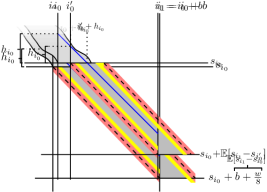
Figure 6: Situation in Cases 1 (left) of 2 (right) of the proof of 1.

•[Case 2: $\bm{h_{i₀}≥\frac{5}{8}w}$.] We claim that all keys belonging to the tail of $B₁$ can be inserted and that afterwards (P1) and (P2) are fulfilled with probability $1-\mathcal{O}(w^{-3})$. In case the keys in the head of $B₁$ can also be successfully inserted this cannot hurt (P1) or (P2) because the number of filled slots and the height could only increase due to the additional keys.

The situation is illustrated in Figure 6 on the right. We only consider the keys in the tail of $B₁$ which starts at position $i₀^{\prime}+1$ where $i₀^{\prime}=i₀+\frac{3}{8}w$. Note that for $i∈[i₀,i₀^{\prime}]$ the ribbon diagonal $(d_{i},i)$ follows an ideal diagonal trajectory with probability $1-\mathcal{O}(2^{-Ω(w)})$ since keys from $B₀$ are successfully inserted and the distance to the bottom border is at least $\frac{1}{4}w$. This implies that all slots in the head of $B₁$ are filled by keys from $B₀$ and $h_{i₀^{\prime}}=h_{i₀}-\frac{3}{8}w$. Since $h_{i₀}∈[\frac{5}{8}w,w]$ we have $h_{i₀^{\prime}}∈[\frac{1}{4}w,\frac{5}{8}w]$, which allows us to reason as in Case $1$ to show that all slots in the tail of bucket $B₁$ are filled and $h_{i₁}≥\frac{w}{4}$ with probability $1-\mathcal{O}(w^{-3})$.

Handling failures and the first bucket.

The following claim is needed to deal with the rare cases where 1 does not apply.

Claim 2.

Assume $B₁$ is either the first bucket, or preceeded by a bucket $B₀$ for which (P2) does not hold. Then with probability $1-\mathcal{O}(w^{-3})$ all keys of $B₁$ (head and tail) are successfully inserted.

Proof 10.3.

The ribbon diagonal $d$ starts at a height $h_{i₀}<\frac{w}{4}$, which is lower than desired, and might hit the lower ribbon border within $B₁$. However, $d$ avoids the right ribbon border, because (recycling ideas from Case 1 of 1) $d$ would have to pierce the diagonal starting at the desired height $\frac{w}{4}$ first and would afterwards stay on that diagonal with probability $1-\mathcal{O}(w^{-3})$. This allows for some slots in $B₁$ to remain empty but implies all keys are successfully inserted with probability $1-\mathcal{O}(w^{-3})$.

We now classify the buckets. Consider a bucket $B₁$. Note that either 1 or 2 is applicable. If the corresponding event with probability $1-\mathcal{O}(w^{-3})$ fails to occur or if $B₁$ contains less than $b$ keys (this happens with probability $\mathcal{O}(w^{-5})$), then $B₁$ is a bad bucket. Otherwise, if 1 applies, then $B₁$ is a good bucket and if 2 applies then $B₁$ is a recovery bucket. A recovery sequence is a maximal contiguous sequence of recovery buckets. Since such a sequence cannot be preceded by a good bucket, the number of recovery sequences is at most the number of bad buckets plus $1$ (the first bucket is always a recovery bucket or bad). Only bad buckets contain fewer than $b$ keys, so a recovery sequence of $k$ buckets contains at least $kb$ keys, all of which are inserted successfully by 2. At most $w-1$ of these insertions fill slots after the sequence so there are at most $w-1$ empty slots within a recovery sequence. With $x$ denoting the number of bad buckets, the number $m-|P_{M}|$ of empty slots in total is

$$m-|P_{M}|≤xb+(x+1)(w-1)+w-1$$

where the last $w-1$ accounts for slots $[m-w+1,m]$ that do not belong to any bucket. The dominating term is $xb$ so using $\mathbb{E}[x]=\mathcal{O}(\frac{m}{b}w^{-3})$ we obtain $\mathbb{E}[\frac{m-|P_{M}|}{m}]=\mathcal{O}(w^{-3})$, which completes the proof of Lemma 10.1.

11 The Design Space of BuRR

There is a large design space for implementing BuRR. We outline it in some breadth because there was a fruitful back-and-forth between different approaches and their analysis, i.e., different approaches gradually improved the final theoretical results while insights gained by the analysis helped to navigate to simple and efficient design points. The description of the design space helps to explain some of the gained insights and might also show directions for future improvements of BuRR. To also accommodate more “hasty” readers, we nevertheless put emphasis on the the main variant of BuRR analyzed Section 10 and also move some details to appendices. We first introduce a simple generic approach and discuss concrete instantiations and refinements in separate subsections. In Appendix A, we describe further details.

As all layers of BuRR function in the same way, we need only explain the construction process of a single layer. The BuRR construction process makes the ribbon retrieval approach of Section 6 more dynamic by bumping ranges of keys when insertion of a row into the linear system fails by causing a linear dependence. Bumping is effected by subdividing the table for the current layer into buckets of size $b$. More concretely, bucket $B$ contains metadata for keys $x$ with $s(x)\in Bb+1..(B+1)b$. We also say that $x$ is allocated to bucket $B$ even though retrieving $x$ can also involve subsequent buckets. In Section 10, we showed that it basically suffices to adaptively remove a fraction of the keys from buckets with high load to make the equation system solvable, i.e., to make all remaining keys retrievable from the current layer. The structure of the linear system easily absorbs most variance within and between buckets but bigger fluctuations are more efficiently handled with bumping.

Construction.

We first sort the keys by the buckets they are allocated to. For simplicity, we set each key’s leading coefficient $\smash{\vec{h}}(x)[s(x)]$ to 1. As the starting positions are distributed randomly, this is not an issue. The ribbon solving approach is adapted to build the row echelon form bucket by bucket from left to right (see Section A.4 for a discussion of variants). Consider now the solution process for a bucket $B$. Within $B$, we place the keys in some order that depends on the concrete strategy; see Section A.1. One useful order is from right to left based on $s(x)$. We store metadata that indicates one or several groups of keys allocated to the bucket that are bumped. These groups correspond to ranges in the placement order, not necessarily from $s(x)$. Which groups can be represented depends on the metadata compression strategy, which we discuss in Sections 11.1 and A.2. For example, in the right-to-left order mentioned above, it makes sense to bump keys $x$ with $s(x)\in Bb+1..Bb+t$ for some threshold $t$, i.e., a leftmost range of slots in a bucket. This makes sense because that part of the bucket is already occupied by keys placed during construction of the previous bucket (see also Figure 3).

If placement fails for one key in a group, all keys in that group are bumped together. Such transactional grouping of insertions is possible by recording offsets of rows inserted for the current group, and clearing those rows if reverting is needed. This implies that we need to record which rows were used by keys of the current group so that we can revert their insertion if needed.

Keys bumped during the construction of a layer are recorded and passed into the construction process of the next layer. Note that additional or independent hashing erases any relationships among keys that led to bumping. In the last layer, we allocate enough space to ensure that no keys are bumped, as in the standard ribbon approach.

Querying. At query time, if we try to retrieve a key $x$ from a bucket $B$, we check whether $x$’s position in the insertion order indicates that $x$ is in a bumped group. If not, we can retrieve $x$ from the current layer, otherwise we have to go on to query the next layer.

Overloading. The tuning parameter $\varepsilon=1-m/n$ is very important for space efficiency. While other linear algebra based retrieval data structures need $\varepsilon>0$ to work, a decisive feature of BuRR is that negative $\varepsilon$ almost eliminates empty table slots by avoiding underloaded ranges of columns.

We discuss further aspects of the design space of BuRR in additional subsections. By default, bucket construction is greedy, i.e., proceeds as far as possible. Section A.3 presents a cautious variant that might have advantages in some cases. Section A.4 justifies our choice to construct buckets from left to right. Section 11.2 discusses how more sparse bit patterns can improve performance. Construction can be parallelized by bumping ranges of $w$ consecutive table slots. This separates the equation system into independent blocks; see Section 11.3. In that section, we also explain external memory construction that with high probability needs only a single scan of the input and otherwise scanning and integer sorting of simple objects. The computed table and metadata can be represented in various forms that we discuss in Section A.5. In particular, interleaved storage allows to efficiently retrieve $f(x)$ one bit at a time, which is advantageous when using BuRR as an AMQ. We can also reduce cache faults by storing metadata together with the actual table entries.

A very interesting variant of BuRR is bump-once ribbon retrieval (Bu¹RR) described in Section 11.4 that guarantees that each key can be found in one of two layers.

11.1 Threshold-Based Bumping

Recall that BuRR places the keys one bucket $B$ at a time and within $B$ according to some ordering – say from right to left defined by a position in $1..b$. A very simple way to represent metadata is to store a single threshold $j_{B}$ that remembers (or approximates) the first time this insertion process fails for $B$ ($j_{B}=0$ if insertion does not fail). During a query, when retrieving a key $x$ that has position $j$ in the insertion process, $x$ is bumped if $j\geq j_{B}$. We need $\log b$ bits if we conflate $b-1$ and $b$ onto $b-1$ and bump the entire bucket. It turns out that for small $r$ (few retrieved bits), the space overhead for this threshold dominates the overhead for empty slots. Thus, we now discuss several ways to further reduce this space.

2-bit Thresholds and $c$-bit Thresholds. metadata implies that we have to choose between four possible thresholds values. It makes sense to have support for threshold values for $j_{B}=0$ (no bumping needed in this bucket) and $j_{B}=b$ (bump entire bucket). The latter is a convenient way to ensure correctness in a nonprobabilistic way, thus obviating restarts with a fresh hash function. The former threshold makes sense because the effect of obliviously bumping some keys from every bucket could also be achieved by choosing a larger value of $\varepsilon$. This leaves two threshold values $\ell$, $u$, as tuning parameters. The experiments in Section 12 use linear formulas of the form $\left\lceil(c_{1}-c_{2}\varepsilon)b\right\rceil$ for $\ell$ and $u$ with the values of $c_{1}$ and $c_{2}$ dependent on $w$, but it also turns out that $u=2\ell$ is a good choice so that the cases $0$, $\ell$, and $2\ell$ can be decoded with a simple linear formula and only the case $j_{B}=b$ needs special case treatment. Moreover, this approach can be generalized to $c$-bit thresholds, where we use $2^{c}-1$ equally spaced thresholds starting at $0$ plus the threshold $b$.

$1^{+}$-Bit Thresholds. The experiments performed for 2-bit thresholds indicated that actually choosing $\ell=u$ performs quite well. Indeed, the analysis in Section 10 takes up this scheme. Moreover, both experiments and theory show that the threshold $b$ (bump entire bucket) occurs only rarely. Hence, we considered compression schemes that store only a single bit most of the time, using some additional storage to store larger bumping thresholds. We slightly deviate from the theoretical setting by allowing arbitrary larger thresholds in order to reduce the space incurred by empty buckets. Thus, we considered a variant where the threshold values $0$ (bump nothing), $t$ (bump something), and also values $t+1..b$ (bump a lot) are possible but where the latter (rare) cases are stored in a separate small hash table $H^{+}$ whose keys are bucket indices.

Compared to 2-bit thresholds, we get a space-time trade-off, however, because accessing the exception table $H^{+}$ costs additional time (even if it is very small and will often fit into the cache). Thus, a further refinement of $1^{+}$-bit thresholds is to partition the buckets into ranges of size $b^{+}$ and to store one bit for each such range to indicate whether any bucket in that range has an entry in $H^{+}$.

11.2 Sparse Bit Patterns

A query to a BuRR data structure as described so far needs to process about $rw/2$ bits of data to produce $r$ bits of output. Despite the opportunity for word parallelism, this can be a considerable cost. It turns out that BuRR also works with significantly more sparse bit patterns. We can split $w$ bits into $k$ groups and set just one randomly chosen bit per group. The downside of sparse patterns is that they incur more linear dependencies. This will induce more bumped keys and possibly more empty slots. Our experiments indicate that the compromise is quite interesting. For example for $w=64$ and $k=8$ we can reduce the expected number of 1-bits by a factor of four and observe faster queries for large $r$ at the cost of a slight increase of space overhead. Figure 5 indicates that our implementation of sparse coefficient BuRR is indeed a good choice for $r\in\{8,16\}$.

11.3 Parallelization and Memory Hierarchies

As a static data structure, queries are trivial to parallelize on a shared-memory system. Parallelizing construction can use (hard) sharding, i.e., subdividing the data structure into pieces that can be built independently. An interesting property of BuRR is that sharding can be done transparently in a way that does not affect query implementation and thus avoids performance overheads for queries. To subdivide the data structure, we set the bumping information in such a way that each piece is delimited by empty ranges of at least $w$ columns in the constraint matrix. This has the effect that the equation system can be solved independently in parallel for ranges of columns separated by such gaps. With the parametrization we choose for BuRR, the fraction of additionally bumped keys will be negligible as long as $n\gg pw^{2}$ where $p$ is the number of threads.

For large BuRRs that fill a significant part of main memory, space consumption during construction can be a major limitation. Once more, sharding is a simple way out – by constructing the data structure one shard at a time, the temporary space overhead for construction is only proportional to the size of a shard rather than to the size of the entire data structure.

An alternative is to consider a “proper” external memory algorithm. The input is a file $F$ of $n$ key–value pairs. The output is a file containing the layers of the BuRR data structure. A difficulty here is that keys could be much larger than $\log n$ bits and that random accesses to keys is much more expensive than just scanning or sorting. We therefore outline an algorithm that, with high probability, reads the key file only once. The trick is to first substitute keys by master hash codes (MHCs) with $c\log n$ bits for a constant $c>2$. Using the well-known calculations for the birthday problem, this size suffices that the MHCs are unique with high probability. If a collision should occur, the entire construction is restarted. Otherwise, the keys are never accessed again – all further hash bits are obtained by applying secondary hash functions to the MHC.

Construction then begins by scanning the input file $F$ and producing a stream $F_{1}$ of pairs (MHC, function value). Construction at layer $i$ amounts to reading a stream $F_{i}$ of MHC–value pairs. This stream $F_{i}$ is then sorted by a bucket ID that is derived from the MHCs. A collision is detected when two pairs with the same MHC show up. These are easy to detect since they will be sorted to the same bucket and the same column within that bucket. Constructing the row echelon form (REM) then amounts to simultaneously scanning $F_{i}$, the REM and the right-hand side. At no time during this process do we need to keep more than two buckets worth of data in main memory. Bumped MHC–value pairs are output as a stream $F_{i+1}$ that is the input for construction of the next layer. Back-substitution amounts to a backward scan of the REM and the right-hand side – producing the table for layer $i$ as an output.

Overall, the I/O complexity is the I/Os for scanning $n$ keys plus sorting $\mathcal{O}\!\left(n\right)$ items consisting of a constant number of machine words ($\mathcal{O}\!\left(\log n\right)$ bits). The fact that there are multiple layers contributes only a small constant factor to the sorting term since these layers are shrinking geometrically with a rather large shrinking factor.

11.4 Bu¹RR: Accessing Only Two Layers in the Worst Case

BuRR as described so far has worst-case constant access time when the the number of layers is constant (our analysis and experiments use four layers). However, for real-time applications, the resulting worst case might be a limitation. Here, we describe how the worst-case number of accessed layers can be limited to two. The idea is quite simple: Rather than mapping all keys to the first layer, we map the keys to all layers using a distribution still to be determined. We now guarantee that a key originally mapped to layer $i$ is either retrieved there or from layer $i+1$. A query for key $x$ now proceeds as follows. First the primary layer $i(x)$ for that key is determined. Then the bumping information of layer $i$ is queried to find out whether $i$ is bumped. If not, $x$ is retrieved from layer $i$, otherwise it is retrieved from layer $i+1$ without querying the bumping information for layer $i+1$.

For constructing layer $i$, the input consists of keys $E^{\prime}_{i}$ bumped from layer $i-1$ ($E^{\prime}_{1}=\emptyset$) and keys $E_{i}$ having layer $i$ as their primary layer ($E_{i}=\emptyset$ for the last layer). First, the bumped keys $E^{\prime}_{i}$ are inserted bucket by bucket. In this phase, a failure to insert a key causes construction to fail. Then the keys $E_{i}$ are processed bucket by bucket as before, recording bumped keys in $E^{\prime}_{i+1}$.

The size of layer $i$ can be chosen as $(1+\varepsilon)(|E^{\prime}_{i}|+|E_{i}|)$ to achieve the same overloading effect as in basic BuRR. An exception is the last layer $i^{*}$ where we choose the size large enough so that construction succeeds with high probability. Note that if $|E_{i}|$ shrinks geometrically, we can choose $i^{*}$ such that $|E_{i^{*}}|$ is negligible.

Except in the last layer, construction can only fail due to keys already bumped, which is a small fraction even for practical $w$. In the unlikely case of construction failing, construction of that layer can be retried with more space. Tests suggest that increasing space by a factor of $\frac{w+1}{w}$ has similar or better construction success probability than a fresh hash function.

A simpler Bu¹RR construction has layers of predetermined sizes, all in one linear system. Construction reliability and/or space efficiency are reduced slightly because of reduced adaptability. For moderate $n\approx w^{3}$, layers of uniform size can work well, especially if the last layer is of variable size.

Our implementation of Bu¹RR, tested to scale to billions of keys, uses layers with sizes shrinking by a factor of two, each with a power of two number of buckets. To a first approximation, the primary layer $i(x)$ of a key is simply the number of leading zeros in an appropriate hash value, up to the maximum layer. To consistently saturate construction with expected overload of $\alpha=-\varepsilon$, this is modified with a bias for the first layer. A portion ($\alpha$) of values with a leading 0 (not first layer) are changed to a leading 1 (re-assigned to first layer), so $|E_{0}|\approx(1+\alpha)2^{-1}m$ and other $|E_{i}|\approx(1-\alpha)2^{-(i+1)}m$. With bumped entries, $|E^{\prime}_{i}|\approx\alpha 2^{-i}m$, expected overload is consistent through the layers: $|E_{i}|+|E^{\prime}_{i}|\approx(1+\alpha)2^{-(i+1)}m$.

12 Experiments

Implementation Details. We implemented BuRR in C++ using template parameters that allow us to navigate a large part of the design space mapped in the full paper. We use sequential construction using 64-bit master-hash-codes (MHCs) so that the input keys themselves are hashed only once. Linear congruential mapping is used to derive more pseudo-random bits from the MHC. When not otherwise mentioned, our default configuration is BuRR with left-to-right processing of buckets, aggressive right-to-left insertion within a bucket, threshold-based bumping, interleaved storage of the solution $Z$, and separately stored metadata. The data structure has four layers, the last of which uses $w^{\prime}:=\min(w,64)$ and $\varepsilon\geq 0$, where $\varepsilon$ is increased in increments of 0.05 until no keys are bumped. For $1^{+}$-bit, we choose $t:=\lceil-2\varepsilon b+\sqrt{b/(1+\varepsilon)}/2\rceil$ and $\varepsilon:=-2/3\cdot w/(4b+w)$. For 2-bit, parameter tuning showed that $\ell:=\left\lceil(0.13-\varepsilon/2)b\right\rceil,u:=\left\lceil(0.3-\varepsilon/2)b\right\rceil$, and $\varepsilon:=-3/w$ work well for $w=32$; for $w\geq 64$, we use $\ell=\left\lceil(0.09-3\varepsilon/4)b\right\rceil$, $u=\left\lceil(0.22-1.3\varepsilon)b\right\rceil$, and $\varepsilon:=-4/w$.

In addition, there is a prototypical implementation of Bu¹RR from [23]; see Section 11.4. Both BuRR and Bu¹RR build on the same software for ribbon solving from [23]. For validation we extend the experimental setup used for Cuckoo and Xor filters [30], with our code available at https://github.com/lorenzhs/fastfilter_cpp and https://github.com/lorenzhs/BuRR.

Experimental Setup. All experiments were run on a machine with an AMD EPYC 7702 processor with 64 cores, a base clock speed of 2.0 GHz, and a maximum boost clock speed of 3.35GHz. The machine is equipped with 1 TiB of DDR4-3200 main memory and runs Ubuntu 20.04. We use the clang++ compiler in version 11.0 with optimization flags -O3 -march=native. During sequential experiments, only a single core was active at any time to minimize interference.

We looked at different input sizes $n\in\left\{10^{6},10^{7},10^{8}\right\}$. Like most studies in this area, we first look at a sequential workload on a powerful processor with a considerable number of cores. However, this seems unrealistic since in most applications, one would not let most cores lay bare but use them. Unless these cores have a workload with very high locality this would have a considerable effect on the performance of the AMQs. We therefore also look at a scenario that might be the opposite extreme to a sequential unloaded setting. We run the benchmarks on all available hardware threads in parallel. Construction builds many AMQs of size $n$ in parallel. Queries select AMQs randomly. This emulates a large AMQ that is parallelized using sharding and puts very high load on the memory system.

Space Overhead of BuRR

Figure 7: Fraction of empty slots for various configurations of bumped ribbon retrieval with $w=64$, depending on the overloading factor $\varepsilon$.

Figure 7 plots the fraction $e$ of empty slots of BuRR for $w=64$ and several combinations of bucket size $b$ and different threshold compression schemes. Similar plots are given in the appendix in Figure 10 for $w=32$, $w=128$, and for $w=64$ with sparse coefficients. Note that (for an infinite number of layers), the overhead is about $o=e+\mu/(rb(1-e))$ where $r$ is the number of retrieved bits and $\mu$ is the number of metadata bits per bucket. Hence, at least when $\mu$ is constant, the overhead is a monotonic function in $e$ and thus minimizing $e$ also minimizes overhead.

We see that for small $|\varepsilon|$, $e$ decreases exponentially. For sufficiently small $b$, $e$ can get almost arbitrarily small. For fixed $b>w$, $e$ eventually reaches a local minimum because with threshold-based compression, a large overload enforces large thresholds ($>w$) and thus empty regions of buckets. Which actual configuration to choose depends primarily on $r$. Roughly, for larger $r$, more and more metadata bits (i.e., small $b$, higher resolution of threshold values) can be invested to reduce $e$. For fixed $b$ and threshold compression scheme, one can choose $\varepsilon$ to minimize $e$. One can often choose a larger $\varepsilon$ to get slightly better performance due to less bumping with little impact on $o$. Perhaps the most delicate tuning parameters are the thresholds to use for 2-bit and $1^{+}$-bit compression (see Section 11.1). Indeed, in Figure 7 $1^{+}$-bit compression has lower $e$ than 2-bit compression for $b=64$ but higher $e$ for $b=128$. We expect that 2-bit compression could always achieve smaller $e$ than $1^{+}$-bit compression, but we have not found choices for the threshold values that always ensure this. Table 4 in Appendix B summarizes key parameters of some selected BuRR configurations.

In all following experiments, we use $b=2^{\lfloor w^{2}/(2\log_{2}w)\rfloor}$ for uncompressed and 2-bit compressed thresholds, and $b=2^{\lfloor w^{2}/(4\log_{2}w)\rfloor}$ when using $1^{+}$-bit threshold compression.

Performance of BuRR Variants

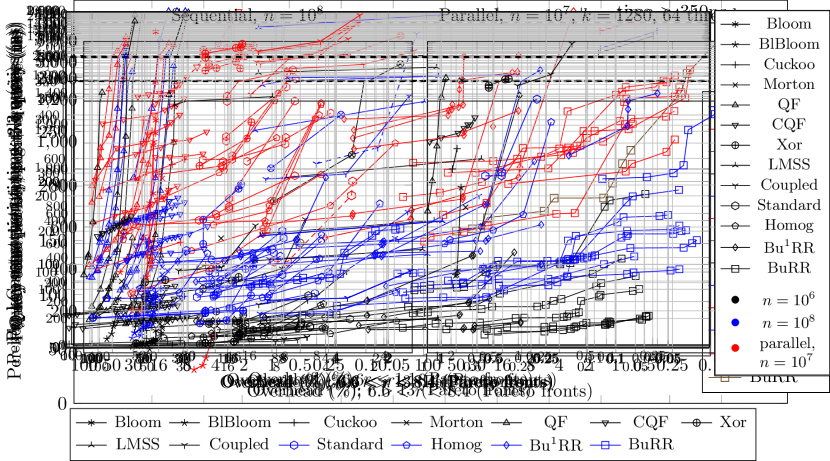
Figure 11: Performance–overhead trade-off for false-positive rate $>46\,\%$ for different AMQs and different inputs. This large false-positive rate is the only one for which we have implementations for GOV [29] and 2-block [19]. Note that the vertical axis switches to a logarithmic scale above 900 ns.

We have performed experiments with numerous configurations of BuRR. See Table 2 in Appendix B for a small sample and Appendix C for the complete list. The scatter plot in Figure 8 summarizes the performance–overhead trade-off for $r\approx 8$. Plots for different values of $r$ and for construction and query times separately are in Appendix B (Figures 11, 12, 13, 14 and 15).

A small ribbon width of $w=16$ is feasible but does not pay off with respect to performance because its high bumping rates drive up the expected number of layers accessed. Choosing $w=32$ yields the best performance in many configurations but the penalty for going to $w=64$ is very small while reducing overheads. In contrast, $w=128$ has a large performance penalty for little additional gain – overheads far below $1\,\%$ are already possible with $w=64$. Thus, on a 64-bit machine, $w=64$ seems the logical choice in most situations.

Figure 8: Performance–overhead trade-off for false-positive rate $2^{-r}$, approximately $0.3\,\%$ to $1\,\%$, for different AMQs and inputs. For each category of approaches, only points are shown that are not dominated by variants in the same category. Sequential benchmarks use a single AMQ of size $n$ while the parallel benchmark uses $1280$ AMQs and 64 cores. Logarithmic vertical axis above 1200 ns.

With respect to performance, 1⁺-bit compression is slightly slower than 2-bit compression or uncompressed thresholds but not by a large margin. However, 1⁺-bit achieves the lowest overheads. Interleaved table representation (see Section A.5) is mostly faster than contiguous representation. This might change for sufficiently large $r$ and use of advanced bit-manipulation or SIMD instructions. Nevertheless, sparse coefficients with 8 out of 64 bits using contiguous representation achieve significantly better query performance than the best dense variant with comparable or better overhead when contiguous storage is efficiently addressable, i.e., $r$ is a multiple of 8.

Bu¹RR is around 20 % slower than BuRR and also somewhat inferior with respect to the achieved overheads. This may in part be due to less extensive parameter tuning. When worst-case guarantees matter, Bu¹RR thus might be a good choice.

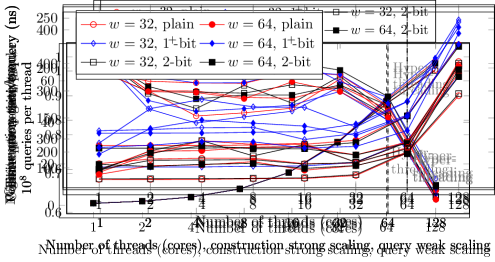
(b) Scaling behavior of positive queries on the filters from (a). Each query accesses a randomly chosen filter. Tested with $10^{8}$ queries per thread.

(c) Scaling behavior of negative queries on the filters from (a). Each query accesses a randomly chosen filter. Tested with $10^{8}$ queries per thread.

Figure 16: Scaling experiments for parallel construction and querying of BuRR.

In a parallel scaling experiment with $10^{10}$ keys, construction and queries both scaled well, shown in Figure 16 in Appendix B. Constructing many AMQs in parallel achieves speedups of $65-71$ depending on the configuration when using all 64 cores plus hyperthreads of our machine (50 without hyperthreading). Individual query times are around $15\,\%$ higher than sequentially when using all cores, and $50\,\%$ higher when using all hyperthreads. This approximately matches the speedups for construction.

Comparison with Other Retrieval and AMQ Data Structures

To compare BuRR with other approaches, we performed an extensive case study of different AMQs and retrieval data structures. To compare space overheads, we compare $r$-bit retrieval data structures to AMQs with false positive rate $2^{-r}$. Our benchmark extends the framework used to evaluate Cuckoo and Xor filters [30], with our modified version available at https://github.com/lorenzhs/fastfilter_cpp. In addition to adding our implementations of standard ribbon, homogeneous ribbon, BuRR, and Bu¹RR, we integrated existing implementations of Quotient Filters [39, 40] and LMSS, Coupled, GOV, 2-block, and BPZ retrieval [49, 50]. We extended the implementations of LMSS, Coupled, and BPZ to support the cases of $r=8$ and $r=16$ in addition to one-bit retrieval.

We also added a parallel version of the benchmark where each thread constructs a number of AMQs independently, but queries access all of them randomly. In the Cuckoo filter implementation, we replaced calls to rand() with a std::mt19937 Mersenne Twister to eliminate a parallel bottleneck. The implementation of LMSS cannot be run simultaneously in multiple threads of the same process and was excluded from the parallel benchmark.

Both the sequential and the parallel benchmark use three query workloads: positive queries, negative queries, and a mixed set containing equal numbers of positive and negative queries. We report many results in the form of construction time per key plus the time for one query from each of the three sets, measured by dividing the running time for construction plus $n$ queries of each type by the input size $n$. This metric is a reasonable tradeoff between construction and queries; we provide figures for the individual components in Appendix B (Figures 13, 14 and 15).

Once more, the scatter plot in Figure 8 summarizes the performance–overhead trade-off for $r\approx 8$; other values of $r$ are covered in Appendix B (Figures 11 and 12). In addition, Figure 5 gives an overview of the fastest approach for different values of $r$ and overhead. We now discuss different approaches progressing from high to low space overhead.

Bloom Filters Variants: Plain Bloom filters [7] set $k\sim\log(1/\varphi)$ random bits in a table for each key in order to achieve false-positive rate $\varphi$. They are the most well-known and perhaps most widely used AMQ. However, they have an inherent space overhead of at least 44 % compared to the information-theoretic optimum. Moreover, for large inputs they cause almost $k$ cache faults for each insertion and positive query. Blocked Bloom filters [47] are faster because they set all of the $k$ bits in the same cache block. The downside is that this increases the false-positive rate, in particular for large $k$. This can be slightly reduced using two blocks.

Cuckoo Filters [25] store a random fingerprint for each key (similar to retrieval-based AMQs). However, to allow good space efficiency, several positions need to be possible. This introduces an intrinsic space overhead of a few bits per key that is further increased by some empty slots that are required to allow fast insertions. The latter overhead is reduced in Morton filters [11] which can be viewed as a compressed representation of cuckoo filters. In our measurements, cuckoo and Morton filters are the most space efficient dynamic AMQ for small $\varphi$, but are otherwise outperformed by other constructions.

Quotient Filters (QF) [5] can be viewed as a compressed representation of a Bloom filter with a single hash function. QFs support not only insertions but also deletions and counting. Similar to cuckoo filters, they incur an overhead of a few bits per key (2–3 depending on the implementation) plus a multiplicative overhead due to empty entries. Search time grows fairly quickly as the multiplicative overhead approaches zero. Counting Quotient Filters (CQF) [45] mitigate this dependence at the cost of less locality for low fill degrees. Overall, quotient filters are good if their rich set of operations is needed but cannot compete with alternatives (e.g., blocked Bloom filters and cuckoo filters) for dynamic AMQs without deletions. Compared to static AMQs, they have comparable or slower speed than BuRR but two orders of magnitude higher overhead.

Xor filter/retrieval. Xor Filters and Xor+ Filters [31] are a recent implementation of peeling-based retrieval that can reduce overhead to 23 % and 14 %, respectively. An earlier implementation [10] is 35–90 % slower to construct and also has slightly slower queries. Fuse filters [20], a variant of Xor, achieve higher loads and are fast to construct if $n$ is not too large, but construction becomes slow for large $n$ and parallel queries are less efficient than for plain Xor filters. In the plots we only show the Pareto-optimal variants in each case and call all of them Xor in the following and in Section 1. Among the tried retrieval data structures, Xor has the fastest queries for sequential settings but is otherwise dominated by BuRR, which has one to two orders of magnitude smaller overheads.

Low overhead peeling-based retrieval. By using several hash functions in a nonuniform way, peeling-based retrieval data structures can in principle achieve arbitrarily small overheads and thus could be viewed as the primary competitors of ribbon-based data structures. LMSS [38] was originally proposed as an error-correcting code but can also be used for retrieval. However, in the experiments it is clearly dominated by BuRR. The more recent Coupled peeling approach [51] can achieve Pareto-optimal query times for large sequential inputs but is otherwise dominated by ribbon-based data structures. Coupled has faster construction times than LMSS but in that respect is several times slower than BuRR for large $n$ and in our parallel benchmark, even when it is allowed an order of magnitude more overhead. Nevertheless, when disregarding ribbon-based data structures, Coupled comes closest to a practical retrieval data structure with very low overhead. For small inputs ($n=10^{6}$), $r\approx 16$ and overhead between 8 and 15 %, it is even the fastest AMQ in our benchmark (see Figure 5). Perhaps for large $r$ and by engineering faster construction algorithms, Coupled could become more competitive in the future.

Standard Ribbon can achieve overhead around 10 %. However, it often fails for large $n$, requiring larger space overhead when used without sharding on top of it. For AMQs this can be elegantly remedied using homogeneous ribbon filters. Thus, in the heatmap, homogeneous ribbon occupies the area between (blocked) Bloom filters and BuRR and its variants. However, the performance advantage over BuRR in parallel and large settings is not very large (typically 20 %).

BuRR and its variants take the entire right part of the heatmap. Compared to the best competitor – homogeneous ribbon filters – overhead drops from around 10 % to well below 1 % at a moderate performance penalty. In particular, due to BuRR’s high locality, performance is even better than for successful competitors like Xor, Cuckoo, or Bloom filters.

2-block [19] can be viewed as a generalization of ribbon-based approaches that use two rather than one block of nonzeroes in each row of the constraint matrix. Unfortunately this makes the equation system much more difficult to solve. This implies very expensive construction even when aggressively using the sharding trick. In our experiments, an implementation by Walzer [50] for $r=1$ achieves smaller overhead than BuRR with $w=128$ at the price of an order of magnitude larger construction time. It is however likely that a BuRR implementation able to handle $w=256$ would dominate 2-block.

Techniques not tried. There are a few interesting retrieval data structures for which we had no available implementation. FiRe [44] is likely to be the fastest existing retrieval data structure and also supports updates to function values as well as a limited form of insertions. FiRe maps keys to buckets fitting into a cache line. Per-bucket metadata is used to uniquely map some keys to data slots available in the bucket while bumping the remaining keys. This requires a constant number of metadata bits per key (around 4) and thus implies an overhead two orders of magnitude larger than BuRR. Additionally, the only known implementation of FiRe is closed source and owned by SAP, and was not available to us.

We are not aware of implementations of the lookup-table based approaches [46, 4] and do not view them as practically promising for the reasons discussed in Section 5.

13 Conclusion and Future Work

BuRR is a considerable contribution to close a gap between theory and practice of retrieval and static approximate membership data structures. From the theoretical side, BuRR is succinct while achieving constant access cost for small number of retrieved bits ($r=\mathcal{O}\!\left(\log(n)/w\right)$). In contrast to previous succinct constructions with better asymptotic running times, its overhead is tunable and already small for realistic values of $n$. In practice, BuRR is faster than widely used data structures with much larger overhead and reasonably simple to implement. Our results further strengthen the success of linear algebra based solutions to the problem. Our on-the-fly approach shows that Gauss-like solvers can be superior to peeling based greedy solvers even with respect to speed.

While the wide design space of BuRR leaves room for further practical improvements, we see the main open problems for large $r$. In practice, peeling based solvers (e.g., [51]) might outperform BuRR if faster construction algorithms can be found – perhaps using ideas like overloading and bumping. In theory, existing succinct data structures (e.g. [46, 4]) allow constant query time but have high space overhead for realistic input sizes. Combining constant cost per element for large $r$ with small (preferably tunable) space overhead therefore remains a theoretical promise yet to be convincingly redeemed in practice.

Acknowledgements

We thank Martin Dietzfelbinger for early contributions to this line of research. We thank others at Facebook for their supporting roles, including Jay Zhuang, Siying Dong, Shrikanth Shankar, Affan Dar, and Ramkumar Vadivelu.

Appendix A More on the Design Space of BuRR

A.1 Different Insertion Orders Within a Bucket

Right-to-left. Assuming that we process buckets from left to right (see also Section A.4), a simple and useful insertion order within a bucket is from right to left, i.e., by decreasing values of $s(x)$. This ordering takes into account that the leftmost part of the bucket is already mostly filled with keys spilled over from the previous bucket whereas the next bucket is still empty. Thus, proceeding from the right to the left, placement is initially easy. With overloaded buckets (negative $\varepsilon$), placement gets more and more difficult and gradually needs to place more and more keys in the next bucket. The analysis in Section 10 suggests that linear dependencies mostly occur in two ways. Either, when the overload of this bucket (or some subrange of it) is too large, or when it runs into the keys placed into the left part of the bucket when the previous bucket was constructed. We make the former event unlikely by choosing appropriate values of $b$ and $\varepsilon$. When the latter event happens, we can bump a range of keys allocated to the leftmost range of the bucket. This bumping scheme is discussed in Section 11.1. The right-to-left ordering then helps us to find the right threshold value. An illustration is shown in Figure 3.

(Quasi)random order. The above simple insertion order is limited to situations where the overload per bucket is less than $w$ most of the time. Otherwise, placement will often fail early, bumping many keys that could actually be placed because their $s$ falls into a range of slots that remain empty. We can achieve more flexibility in choosing $\varepsilon$ by spreading keys more uniformly over the bucket during the insertion process. We tried several such approaches. Bu¹RR uses additional hash bits to make the ordering for bumping independent of the position within the bucket. Another interesting variant is most easy to explain when $b$ is a power of two. We use $c=\log b$ bits of hash function value to define the position within a bucket. However, rather than directly using the value as a column number, we use its mirror image, i.e., a value $h_{c-1}h_{c-2}\ldots h_{1}h_{0}$ addresses column $h_{0}h_{1}\ldots h_{c-2}h_{c-1}$ of a bucket. We also tried a tabulated random permutation, which according to early experiments, works slightly worse than the mirror permutation.

A.2 Metadata for Bumping Multiple Groups

A disadvantage of threshold-based bumping is that a single failed placement of a key implies that all subsequently placed keys allocated to that bucket must be bumped. This penalty can be mitigated by subdividing the positions in the insertion order into multiple groups that can be bumped separately, e.g., by storing a single bit that indicates whether a group is bumped. Choosing groups of uniform (expected) size is simple and fast. It works well when highly compressed metadata is not of primary importance, e.g., when $r$ is large.

Better compression can be achieved by choosing groups of variable size. Bu¹RRs use groups whose sizes are a geometric progression with a factor about $\sqrt{2}$ between subsequent group sizes. For example, to cover a bucket of size $b=1024$ using 8 bits of metadata, one could use groups of expected sizes 28, 40, 57, 80, 113, 160, 226, and 320. Note that smaller groups cannot and need not be bumped since the main effect of bumping “too much” is that fewer keys spill over to the next bucket which can be rectified there. This is also the underlying reason why highly compressed representations of the threshold metadata from Section 11.1 are sufficient.

A.3 Aggressive versus Cautious Bumping

By default, the generic BuRR solving approach described in Section 11 is greedy, i.e., it tries to place as many keys as possible into the current bucket. This will usually spill over close to $w$ keys into the next bucket. This increases the likelihood that construction in that bucket fails early. It might be a better approach to be more cautious and try to avoid this situation. For example, when after processing a column $j$, more than $\alpha w$ keys are already placed in the next bucket then all further keys are bumped from the current bucket. More sophisticated balancing approaches are conceivable.

For example, we use a form of cautious bumping for our implementation of Bu¹RR (see Section 11.4). After placing keys bumped from the previous layer, when processing bucket $i$, we first try to place keys in its largest group. Then we try to place the keys in the second largest group in bucket $i-1$, the third largest group in bucket $i-2$, etc. This can be viewed as driving a “wedge” through the buckets.

A.4 Different Global Insertion Orders

Many of our implemented variants of BuRR process buckets from left to right and, within a bucket, place keys $x$ from right to left with respect to $s(x)$. We also tried the dual approach – traversing the buckets from right to left and then inserting from left to right within a bucket. This behaves identically with respect to space efficiency but leads to far more row operations and much higher construction times. The straightforward ordering from left to right both between and inside buckets does not work well with aggressive bumping – placement frequently fails early. We expect that it may turn out to be a natural order for a cautious bumping strategy. Many other insertion orders can be considered. However, the global left-to-right order has the advantage that spilling keys to the next bucket is cheap since it is still empty. Thus, other orders might have higher insertion time.

A.5 Table Representation

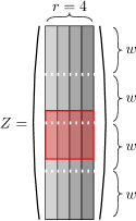
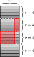
Figure 9: A solution matrix (left) and $w$-bit interleaved column-major layout (right) of that matrix. The red shaded region shows the bits used in a query crossing a boundary.

Interleaved Versus Contiguous Storage. Contiguous storage is the “obvious” representation of the table by $m$ slots of $r$ contiguous bits each. Interleaved means that the table is organized as $rm/w$ words of $w$ bits each where word $i$ represents bit $i\bmod r$ of $w$ subsequent table entries [23]. This organization allows the extraction of one retrieved bit from two adjoining machine words using population-count instructions. Interleaved representation is advantageous for uses of BuRR as an AMQ data structure since a negative query only has to extract two bits in expectation. Moreover, the implementation directly works for any value of $r$.

The contiguous representation, despite its conceptual simplicity, is more difficult to implement, in particular when $r$ is not a power of two. On the other hand, we expect it to be more efficient when all $r$ bits need to be retrieved, in particular when $r$ is large and when the implementation makes careful use of available bit-manipulation and SIMD instructions. This is particularly true when the sparse bit patterns from Section 11.2 are used.

Embedded Versus Separate Metadata. The “obvious” way to represent metadata is as a separate array with one entry for each bucket (and a separate hash table for the $1^{+}$-bit representation). On the other hand, if the metadata cannot be assumed to be resident in cache, it is more cache-efficient to store one bucket completely in one cache line, holding both its table entries and metainformation. Then, assuming $b\geq w$, querying the data structure accesses only one cache line plus possibly the next cache line when the accessed part of the table extends there. In preliminary experiments with variants of this approach, we observed performance improvements of up to 10 % in some cases. We believe that, depending on the implementation and the use case, the difference could also be bigger but have not investigated this further since there are too many disadvantages to this approach: In particular, in the most space-efficient configurations of BuRR, buckets can be bigger than a cache line and the metadata will often fit into cache anyway. Furthermore, when the memory system is not too contended, metadata and primary table can be accessed in parallel, thus eliminating the involved overhead. Finally, embedded metadata is more complicated to implement.

Appendix B Further Experimental Data

The following figures and tables contain

•[Figure 10.] Shows the fraction of empty slots for many BuRR variants, supplementary to Figure 7. •[Figures 11 and 12.] Performance-overhead trade-off of AMQs for very high false positive rate ($≈50\%$) and very low false positive rate ($≈0.01\%$) roughly corresponding to performance of $1$-bit retrieval and $16$-bit retrieval for the retrieval-based AMQs. •[Figures 13, 14 and 15.] Performance-overhead trade-off of AMQs as in Figure 8, but seperately for positive queries, negative queries and construction. •[Figure 16.] Experiments concerning parallel scaling. •[Tables 2 and 3.] Numerical display of selected data. •[Table 4.] Overloading factors used for various BuRR configurations and corresponding overhead.

(a) Ribbon width $w=32$, regular (dense) coefficient vectors.

(b) Ribbon width $w=128$, regular (dense) coefficient vectors.

(c) Ribbon width $w=64$, sparse coefficient vectors with 8 out of 64 positions occupied.

Figure 10: Fraction of empty slots for various configurations of BuRR, depending on the overloading factor $\varepsilon$.

Table 2: Experimental performance comparisons. Overhead, construction and query times (positive and negative queries) for various AMQs. Tested configurations: $n=10^{6}$ keys, $n=10^{8}$ keys, both sequential, as well as 1280 AMQs with $n=10^{7}$ keys each (total: $1.28\times 10^{10}$ keys), constructed and queried in parallel using 64 threads, with each query operating on a randomly chosen AMQ.

	Space	ns/key, $n=10^{6}$			ns/key, $n=10^{8}$			parallel, $n\!=\!10^{7}$
Configuration	ovr %	con	pos	neg	con	pos	neg	con	pos	neg
$\downarrow\,\,$ False positive rate around 1 %, ribbons using $r=7$ $\,\,\downarrow$
Blocked Bloom [36]	52.0	3	3	3	17	24	24	50	116	101
Blocked Bloom [22]	49.8	7	4	4	50	26	26	78	109	85
Blocked Bloom [22] $k=2$	45.0	9	7	7	57	43	43	110	149	194
Cuckoo12 [25] $\dagger$	46.3	29	10	7	118	56	52	239	162	282
Cuckoo12 [25]	40.4	35	12	7	166	58	51	288	180	271
Morton [11]	40.6	32	25	22	64	96	87	130	182	203
Xor [31] $r=7$ $\ddagger$	23.0	91	8	8	169	56	56	644	333	348
Xor [31] $r=8$	23.0	91	5	5	159	41	41	586	386	392
Xor+ [31] $r=8$	14.4	94	14	15	209	86	85	853	372	475
XorFuse [20] $r=8$	16;14	89	6	6	215	43	44	453	532	534
LMSS [38] $D\!=\!12,c\!=\!0.91,r\!=\!8$	11.1	421	28	28	779	134	134	not tested
LMSS [38] $D\!=\!150,c\!=\!0.99,r\!=\!8$	1.0	464	34	34	877	152	152	not tested
Coupled [51] $k=4,r=8$	8;4	104	9	9	229	59	59	546	579	578
Coupled [51] $k=7,r=8$	6;2	169	12	12	331	91	91	813	1337	1342
Quotient Filter [5]	81.9	69	432	272	114	225	169	133	385	308
Counting Quotient Filter [45]	67;55	60	45	31	172	153	113	183	307	252
Standard Ribbon $w=64$	14;20	32	16	20	70	78	66	324	234	194
Standard Ribbon $w=128$	6;8	69	24	25	121	140	87	464	296	206
Homog. Ribbon $w=16$	52.2	19	14	20	42	73	61	69	148	128
Homog. Ribbon $w=32$	20.7	20	13	19	50	73	60	105	147	168
Homog. Ribbon $w=64$	9.9	28	14	19	67	75	63	155	164	170
Homog. Ribbon $w=128$	4.9	58	21	23	118	135	85	306	292	208
Bu1RR $w=32\dagger$	10.3	40	21	26	94	125	88	163	275	286
Bu1RR $w=32$	2.4	62	21	26	121	123	88	174	261	239
BuRR plain $w=32$	1.4	76	20	26	81	82	79	151	247	210
BuRR 2-bit $w=32$	1.3	77	19	26	82	82	80	152	233	245
BuRR $1\kern-1.49994pt^{+}$-bit $w=32$	0.82	80	29	34	84	88	88	158	240	231
Bu1RR $w=64$	0.62	121	21	26	188	128	90	197	292	300
BuRR plain $w=64$	0.48	109	18	24	115	82	74	182	229	213
BuRR 2-bit $w=64$	0.25	110	19	24	115	82	74	190	215	215
BuRR $1\kern-1.49994pt^{+}$-bit $w=64$	0.21	110	27	33	115	86	84	189	238	228
Bu1RR $w=128$	0.31	332	29	30	442	147	100	427	369	285
BuRR plain $w=128$	0.18	209	27	27	214	141	88	319	317	226
BuRR 2-bit $w=128$	0.10	186	27	27	191	140	88	294	313	211
BuRR $1\kern-1.49994pt^{+}$-bit $w=128$	0.06	208	34	37	214	142	92	304	319	235
$\dagger$ Larger space allocated to improve construction time.
$\ddagger$ Potentially unfavorable bit alignment.
; Standard Ribbon, XorFuse, Coupled, and CQF space overhead depend on $n$.

Table 3: Experimental performance comparisons (continued from Table 2).

	Space	ns/key, $n=10^{6}$			ns/key, $n=10^{8}$			parallel, $n=10^{7}$
Configuration	ovr %	con	pos	neg	con	pos	neg	con	pos	neg
$\downarrow\,\,$ False positive rate around 10 %, ribbons using $r=3$ $\,\,\downarrow$
Xor [31] $r=3\ddagger$	23.0	91	6	6	169	51	51	633	292	270
Standard Ribbon $w=64$	14;20	27	9	9	65	54	51	326	118	138
Standard Ribbon $w=128$	6;8	62	14	14	114	67	67	467	139	191
Homog. Ribbon $w=16$	34.6	16	9	9	40	58	59	67	141	140
Homog. Ribbon $w=32$	16.1	17	8	8	49	45	45	101	153	151
Homog. Ribbon $w=64$	8.0	24	8	8	65	45	45	158	132	145
Homog. Ribbon $w=128$	4.0	57	13	13	119	65	65	324	162	193
Bu1RR $w=32$	2.8	60	14	14	119	67	67	175	193	212
BuRR plain $w=32$	3.2	73	14	21	78	64	64	145	180	170
BuRR 2-bit $w=32$	2.5	74	14	21	79	64	65	147	227	214
BuRR $1\kern-1.49994pt^{+}$-bit $w=32$	1.6	77	23	30	82	67	74	150	202	215
Bu1RR $w=64$	0.8	118	13	13	187	66	67	195	192	220
BuRR plain $w=64$	1.1	104	13	20	110	63	62	177	160	172
BuRR 2-bit $w=64$	0.6	106	13	21	111	64	64	188	174	181
BuRR $1\kern-1.49994pt^{+}$-bit $w=64$	0.4	106	22	29	111	66	71	189	196	221
$\downarrow\,\,$ False positive rate around $\mathbf{2^{-11}\approx 0.05\,\%}$, ribbons using $r=11$ $\,\,\downarrow$
Cuckoo16 [25]	30.1	31	11	7	156	56	50	309	180	294
Cuckoo16 [25] $\dagger$	35.7	28	10	7	119	56	44	243	188	308
CuckooSemiSort	26.6	64	15	14	259	79	79	376	264	326
Morton [11]	36.8	38	40	35	69	167	156	127	314	305
Xor [31] $r=12$	23.0	89	8	7	163	57	57	632	415	435
Xor+ [31] $r=11\ddagger$	12.8	98	16	16	215	101	99	759	470	494
Quotient Filter [5]	93.6	71	485	304	109	235	175	138	402	324
Standard Ribbon, $w=64$	14;20	38	23	21	76	143	69	342	294	205
Standard Ribbon, $w=128$	6;8	71	33	26	124	158	91	442	336	243
Homog. Ribbon, $w=32$	28.5	24	18	20	53	82	63	109	230	179
Homog. Ribbon, $w=64$	12.1	32	18	20	70	86	65	165	218	195
Homog. Ribbon, $w=128$	6.5	58	30	25	115	155	89	281	333	305
Bu1RR, $w=32$	2.4	66	28	27	125	152	92	178	405	277
BuRR plain $w=32$	0.94	81	28	26	86	145	83	149	327	229
BuRR 2-bit $w=32$	0.95	82	27	26	87	145	81	150	328	217
BuRR $1\kern-1.49994pt^{+}$-bit $w=32$	0.61	85	35	35	90	148	92	158	352	220
Bu1RR, $w=64$	0.57	128	28	27	196	152	95	203	400	296
BuRR plain $w=64$	0.32	116	27	25	121	146	79	175	334	250
BuRR 2-bit $w=64$	0.17	118	27	25	123	146	77	164	328	209
BuRR $1\kern-1.49994pt^{+}$-bit $w=64$	0.14	115	33	34	120	147	90	189	353	239
BuRR plain $w=128$	0.13	214	35	28	220	159	92	305	364	244
BuRR 2-bit $w=128$	0.08	202	35	28	208	159	92	297	358	226
BuRR $1\kern-1.49994pt^{+}$-bit $w=128$	0.05	214	42	38	219	160	96	317	389	294
$\dagger$ Larger space allocated to improve construction time.
$\ddagger$ Potentially unfavorable bit alignment.
; Standard Ribbon space overhead depends on $n$.

Table 4: Selected BuRR configurations for various $r$. Sparse coefficient vectors used for rows with threshold compression mode marked ^s.

			thresh	overloading	empty	metabits	estimated
$r$	$w$	$b$	mode	factor $\varepsilon$	slots (%)	/bucket	overhead (%)
1	128	512	$1\kern-1.49994pt^{+}$-bit	-0.0470588	0.017477	1.3194	0.275219
1	64	256	2-bit	-0.034375	0.442091	2	1.226810
1	64	128	2-bits	-0.05625	0.261241	2	1.827833
1	32	64	2-bit	-0.08125	0.681598	2	3.828044
2	128	512	$1\kern-1.49994pt^{+}$-bit	-0.0470588	0.017477	1.3194	0.146348
2	64	128	$1\kern-1.49994pt^{+}$-bit	-0.0888889	0.062375	1.2511	0.551393
2	64	128	2-bit	-0.08125	0.013288	2	0.794642
2	64	128	2-bits	-0.05625	0.261241	2	1.044537
2	32	64	2-bit	-0.08125	0.681598	2	2.254821
4	128	512	$1\kern-1.49994pt^{+}$-bit	-0.0431373	0.008797	1.4402	0.079125
4	64	128	2-bit	-0.08125	0.013288	2	0.403965
4	64	128	2-bits	-0.05625	0.261241	2	0.652889
4	32	64	2-bit	-0.08125	0.681598	2	1.468210
8	128	512	$1\kern-1.49994pt^{+}$-bit	-0.0431373	0.008797	1.4402	0.043961
8	64	128	2-bit	-0.08125	0.013288	2	0.208626
8	64	128	2-bits	-0.05625	0.261241	2	0.457065
8	32	64	2-bit	-0.08125	0.681598	2	1.074904
16	128	512	$1\kern-1.49994pt^{+}$-bit	-0.0411765	0.007102	1.5117	0.025557
16	64	128	2-bit	-0.08125	0.013288	2	0.110957
16	64	64	2-bits	-0.065625	0.109362	2	0.304888
16	32	64	plain	-0.13125	0.046154	6	0.632362

Figure 12: Performance–overhead trade-off for false-positive rate $<2^{-13}\approx 0.01\,\%$ for different AMQs and different inputs. Logarithmics vertical axis above 1600 ns.

Figure 13: Query time–overhead trade-off for positive queries, false-positive rate between $0.3\,\%$ and $1\,\%$ for different AMQs and different inputs. Note that Xor filters have excellent query time sequentially where random fetches can be performed in parallel but are far from optimal in the parallel setting where the total number of memory accesses matters most. Logarithmic vertical axis above 350 ns.

Figure 14: Query time–overhead trade-off for negative queries, false-positive rate between $0.3\,\%$ and $1\,\%$ for different AMQs and different inputs. Again, Xor filters perform well sequentially but suffer in the parallel case. Logarithmic vertical axis above 350 ns.

Figure 15: Construction time–overhead trade-off for false-positive rate between $0.3\,\%$ and $1\,\%$ for different AMQs and different inputs. Compressed vertical axis above 350 ns.

(a) Construction of $10\,000$ filters with $10^{6}$ keys each ($w=32$) or $5\,000$ filters with $2\cdot 10^{6}$ keys each ($w=64$), for a total of $10^{10}$ keys; strong scaling.

Appendix C Full Experimental Results

LABEL:tbl:full1 and LABEL:tbl:full2 below contain the results of our performance experiments for all tested configurations for the experiments of Section 12, first for retrieval-based approaches in LABEL:tbl:full1, and then for AMQ data structures in LABEL:tbl:full2.

References

- [1] Martin Aumüller, Martin Dietzfelbinger, and Michael Rink. Experimental variations of a theoretically good retrieval data structure. In Proc. 17th ESA, pages 742–751, 2009. doi:10.1007/978-3-642-04128-0_66.
- [2] Michael Axtmann, Sascha Witt, Daniel Ferizovic, and Peter Sanders. Engineering in-place (shared-memory) sorting algorithms. CoRR, 2020. arXiv:2009.13569.
- [3] Djamal Belazzougui, Paolo Boldi, Giuseppe Ottaviano, Rossano Venturini, and Sebastiano Vigna. Cache-oblivious peeling of random hypergraphs. In Proc. DCC, pages 352–361, 2014. doi:10.1109/DCC.2014.48.
- [4] Djamal Belazzougui and Rossano Venturini. Compressed static functions with applications. In Sanjeev Khanna, editor, Proc. 24th SODA, pages 229–240. SIAM, 2013. doi:10.1137/1.9781611973105.17.
- [5] Michael A. Bender, Martin Farach-Colton, Rob Johnson, Russell Kraner, Bradley C. Kuszmaul, Dzejla Medjedovic, Pablo Montes, Pradeep Shetty, Richard P. Spillane, and Erez Zadok. Don’t thrash: How to cache your hash on flash. Proc. VLDB Endow., 5(11):1627–1637, 2012. doi:10.14778/2350229.2350275.
- [6] Valerio Bioglio, Marco Grangetto, Rossano Gaeta, and Matteo Sereno. On the fly gaussian elimination for LT codes. Communications Letters, IEEE, 13(12):953 – 955, 12 2009. doi:10.1109/LCOMM.2009.12.091824.
- [7] Burton H. Bloom. Space/time trade-offs in hash coding with allowable errors. Commun. ACM, 13(7):422–426, 1970. doi:10.1145/362686.362692.
- [8] Fabiano Cupertino Botelho. Near-Optimal Space Perfect Hashing Algorithms. PhD thesis, Federal University of Minas Gerais, 2008. URL: http://cmph.sourceforge.net/papers/thesis.pdf.
- [9] Fabiano Cupertino Botelho, Rasmus Pagh, and Nivio Ziviani. Simple and space-efficient minimal perfect hash functions. In Proc. 10th WADS, pages 139–150, 2007. doi:10.1007/978-3-540-73951-7_13.
- [10] Fabiano Cupertino Botelho, Rasmus Pagh, and Nivio Ziviani. Practical perfect hashing in nearly optimal space. Inf. Syst., 38(1):108–131, 2013. doi:10.1016/j.is.2012.06.002.
- [11] Alex D. Breslow and Nuwan Jayasena. Morton filters: fast, compressed sparse cuckoo filters. VLDB J., 29(2-3):731–754, 2020. doi:10.1007/s00778-019-00561-0.
- [12] Andrei Z. Broder and Anna R. Karlin. Multilevel adaptive hashing. In David S. Johnson, editor, Proc. 1st SODA, pages 43–53. SIAM, 1990. URL: http://dl.acm.org/citation.cfm?id=320176.320181.
- [13] Bernard Chazelle, Joe Kilian, Ronitt Rubinfeld, and Ayellet Tal. The Bloomier filter: An efficient data structure for static support lookup tables. In Proc. 15th SODA, pages 30–39. SIAM, 2004. URL: http://dl.acm.org/citation.cfm?id=982792.982797.
- [14] Colin Cooper. On the rank of random matrices. Random Structures & Algorithms, 16(2):209–232, 2000. doi:10.1002/(SICI)1098-2418(200003)16:2<209::AID-RSA6>3.0.CO;2-1.
- [15] Niv Dayan, Manos Athanassoulis, and Stratos Idreos. Monkey: Optimal navigable key-value store. In Proceedings of the 2017 ACM International Conference on Management of Data, SIGMOD ’17, page 79–94, New York, NY, USA, 2017. Association for Computing Machinery. doi:10.1145/3035918.3064054.
- [16] Martin Dietzfelbinger, Andreas Goerdt, Michael Mitzenmacher, Andrea Montanari, Rasmus Pagh, and Michael Rink. Tight thresholds for cuckoo hashing via XORSAT. In Proc. 37th ICALP (1), pages 213–225, 2010. doi:10.1007/978-3-642-14165-2_19.
- [17] Martin Dietzfelbinger and Rasmus Pagh. Succinct data structures for retrieval and approximate membership (extended abstract). In Proc. 35th ICALP (1), pages 385–396, 2008. doi:10.1007/978-3-540-70575-8_32.
- [18] Martin Dietzfelbinger and Michael Rink. Applications of a splitting trick. In Proc. 36th ICALP (1), pages 354–365, 2009. doi:10.1007/978-3-642-02927-1_30.
- [19] Martin Dietzfelbinger and Stefan Walzer. Constant-time retrieval with extra bits. In Proc. 36th STACS, pages 24:1–24:16, 2019. doi:10.4230/LIPIcs.STACS.2019.24.
- [20] Martin Dietzfelbinger and Stefan Walzer. Dense peelable random uniform hypergraphs. In Proc. 27th ESA, pages 38:1–38:16, 2019. doi:10.4230/LIPIcs.ESA.2019.38.
- [21] Martin Dietzfelbinger and Stefan Walzer. Efficient Gauss elimination for near-quadratic matrices with one short random block per row, with applications. In Proc. 27th ESA, pages 39:1–39:18, 2019. doi:10.4230/LIPIcs.ESA.2019.39.
- [22] Peter C. Dillinger. RocksDB FastLocalBloom, 2019. URL: https://github.com/facebook/rocksdb/blob/master/util/bloom_impl.h.
- [23] Peter C. Dillinger and Stefan Walzer. Ribbon filter: practically smaller than Bloom and Xor. CoRR, 2021. arXiv:2103.02515.
- [24] Olivier Dubois and Jacques Mandler. The 3-XORSAT threshold. In Proc. 43rd FOCS, pages 769–778, 2002. doi:10.1109/SFCS.2002.1182002.
- [25] Bin Fan, David G. Andersen, and Michael Kaminsky. Cuckoo filter: Better than Bloom. ;login:, 38(4), 2013. URL: https://www.usenix.org/publications/login/august-2013-volume-38-number-4/cuckoo-filter-better-bloom.
- [26] Dimitris Fotakis, Rasmus Pagh, Peter Sanders, and Paul G. Spirakis. Space efficient hash tables with worst case constant access time. Theory Comput. Syst., 38(2):229–248, 2005. doi:10.1007/s00224-004-1195-x.
- [27] Nikolaos Fountoulakis and Konstantinos Panagiotou. Sharp load thresholds for cuckoo hashing. Random Struct. Algorithms, 41(3):306–333, 2012. doi:10.1002/rsa.20426.
- [28] Marco Genuzio, Giuseppe Ottaviano, and Sebastiano Vigna. Fast scalable construction of (minimal perfect hash) functions. In Proc. 15th SEA, pages 339–352, 2016. doi:10.1007/978-3-319-38851-9_23.
- [29] Marco Genuzio, Giuseppe Ottaviano, and Sebastiano Vigna. Fast scalable construction of ([compressed] static | minimal perfect hash) functions. Information and Computation, 2020. doi:10.1016/j.ic.2020.104517.
- [30] Thomas Mueller Graf and Daniel Lemire. fastfilter_cpp, 2019. URL: https://github.com/FastFilter/fastfilter_cpp.
- [31] Thomas Mueller Graf and Daniel Lemire. Xor filters: Faster and smaller than Bloom and cuckoo filters. ACM J. Exp. Algorithmics, 25:1–16, 2020. doi:10.1145/3376122.
- [32] Jóhannes B. Hreinsson, Morten Krøyer, and Rasmus Pagh. Storing a compressed function with constant time access. In Proc. 17th ESA, pages 730–741, 2009. doi:10.1007/978-3-642-04128-0_65.
- [33] Svante Janson and Malwina J. Luczak. A simple solution to the -core problem. Random Struct. Algorithms, 30(1-2):50–62, 2007. doi:10.1002/rsa.20147.
- [34] Adam Kirsch and Michael Mitzenmacher. Less hashing, same performance: Building a better Bloom filter. Random Struct. Algorithms, 33(2):187–218, 2008. doi:10.1002/rsa.20208.
- [35] D. E. Knuth. The Art of Computer Programming — Seminumerical Algorithms, volume 2. Addison Wesley, 2nd edition, 1981.
- [36] Harald Lang, Thomas Neumann, Alfons Kemper, and Peter A. Boncz. Performance-optimal filtering: Bloom overtakes cuckoo at high-throughput. Proc. VLDB Endow., 12(5):502–515, 2019. doi:10.14778/3303753.3303757.
- [37] Marc Lelarge. A new approach to the orientation of random hypergraphs. In Proc. 23rd SODA, pages 251–264. SIAM, 2012. doi:10.1137/1.9781611973099.23.
- [38] Michael Luby, Michael Mitzenmacher, Mohammad Amin Shokrollahi, and Daniel A. Spielman. Efficient erasure correcting codes. IEEE Trans. Inf. Theory, 47(2):569–584, 2001. doi:10.1109/18.910575.
- [39] Tobais Maier. lpqfilter, 2020. URL: https://github.com/TooBiased/lpqfilter.
- [40] Tobias Maier, Peter Sanders, and Robert Williger. Concurrent expandable AMQs on the basis of quotient filters. In Proc. 18th SEA, pages 15:1–15:13, 2020. doi:10.4230/LIPIcs.SEA.2020.15.
- [41] Michael Mitzenmacher and Eli Upfal. Probability and Computing: Randomization and Probabilistic Techniques in Algorithms and Data Analysis. Cambridge University Press, New York, NY, USA, 2nd edition, 2017.
- [42] Michael Molloy. Cores in random hypergraphs and Boolean formulas. Random Struct. Algorithms, 27(1):124–135, 2005. doi:10.1002/rsa.20061.
- [43] Ingo Müller, Cornelius Ratsch, and Franz Färber. Adaptive string dictionary compression in in-memory column-store database systems. In Proc. 17th EDBT, pages 283–294, 2014. doi:10.5441/002/edbt.2014.27.
- [44] Ingo Müller, Peter Sanders, Robert Schulze, and Wei Zhou. Retrieval and perfect hashing using fingerprinting. In Proc. 14th SEA, pages 138–149, 2014. doi:10.1007/978-3-319-07959-2_12.
- [45] Prashant Pandey, Michael A. Bender, Rob Johnson, and Rob Patro. A general-purpose counting filter: Making every bit count. In Proc. 2017 SIGMOD, pages 775–787. ACM, 2017. doi:10.1145/3035918.3035963.
- [46] Ely Porat. An optimal Bloom filter replacement based on matrix solving. In Proc. 4th CSR, pages 263–273, 2009. doi:10.1007/978-3-642-03351-3_25.
- [47] Felix Putze, Peter Sanders, and Johannes Singler. Cache-, hash-, and space-efficient Bloom filters. ACM Journal of Experimental Algorithmics, 14, 2009. doi:10.1145/1498698.1594230.
- [48] Kapil Vaidya, Eric Knorr, Tim Kraska, and Michael Mitzenmacher. Partitioned learned bloom filter. CoRR, abs/2006.03176, 2020. URL: https://arxiv.org/abs/2006.03176, arXiv:2006.03176.
- [49] Stefan Walzer. Experimental comparison of retrieval data structures, 2020. URL: https://github.com/sekti/retrieval-test.
- [50] Stefan Walzer. Random Hypergraphs for Hashing-Based Data Structures. PhD thesis, Technische Universität Ilmenau, 2020. URL: https://www.db-thueringen.de/receive/dbt_mods_00047127.
- [51] Stefan Walzer. Peeling close to the orientability threshold: Spatial coupling in hashing-based data structures. In Proc. 32nd SODA, pages 2194–2211. SIAM, 2021. doi:10.1137/1.9781611976465.131.