Straight-line Drawings of 1-Planar Graphs

Abstract

A graph is 1-planar if it can be drawn in the plane so that each edge is crossed at most once. However, there are 1-planar graphs which do not admit a straight-line 1-planar drawing. We show that every 1-planar graph has a straight-line drawing with a two-coloring of the edges, so that edges of the same color do not cross. Hence, 1-planar graphs have geometric thickness two. In addition, each edge is crossed by edges with a common vertex if it is crossed more than twice. The drawings use high precision arithmetic with numbers with $O(n\log n)$ digits and can be computed in linear time from a 1-planar drawing.

1 Introduction

Straight-line drawings of graphs, also known as rectilinear or geometric drawings, are an important topic in Graph Drawing, Graph Theory, and Computational Geometry. The existence of straight-line drawings of planar graphs was discovered by Steinitz and Rademacher [1], Wagner [2], Fáry [3], and Stein [4]. Hence, straight-line is no restriction for planar graphs. The first algorithms for constructing straight-line planar drawings need high precision arithmetic [5, 6, 7, 8]. Later, de Fraysseix et al. [9] and Schnyder [10] showed that planar graphs can be drawn straight-line on a grid of quadratic size. The drawings can be convex, so that the faces are convex polygons if the graphs are 3-connected [11, 12, 13]. However, the produced drawings are not aesthetically pleasing, since they have a low angular resolution.

A drawing (or embedding) of a graph in the plane is 1-planar if each edge is crossed at most once. A graph is 1-planar if it admits such a drawing. Here, straight-line is a real restriction. Thomassen [14] showed that a 1-planar drawing can be transformed into a straight-line 1-planar drawing if and only if it does not contain a B- or a W-configuration, see Fig. 1. This fact was rediscovered by Hong et. al [15]. B- and W-configurations are related to separation pairs, so that there is a pair of crossed edges in the outer face of a component. Didimo [16] showed that straight-line 1-planar drawings of $n$-vertex graphs have at most $4n-9$ edges, whereas there are 1-planar graphs with $4n-8$ edges [17].

(a)

(b)

(c)

Figure 1: (a) A W-configuration with base $(v_{1},v_{2})$, top vertices $t_{1}$ and $t_{2}$ and a first inner face drawn green with a texture, (b) a B-configuration with a pair of crossed edges in the outer face, which in (c) is removed by a flip of the component that changes the embedding.

Straight-line is also a real restriction for fan-crossing [18], fan-crossing free [19, 20], and 2-planar graphs [21], which each generalize 1-planar graphs. Fan-crossing graphs admit drawings with the crossing of an edge by edges of a fan, that is the crossing edges are incident to a common vertex, whereas such crossings are excluded for fan-crossing free graphs [22]. Then only crossings by independent edges are allowed, that is the edges have distinct vertices. Note that there are graphs that are fan-crossing and fan-crossing free, but not 1-planar [23]. Straight-line fan-crossing drawings are fan-planar [24], which are fan-crossing and exclude crossings of an edge from both sides. However, there are fan-crossing graphs that are not fan-planar [18]. A fan-crossing free drawing of an $n$-vertex graph with $4n-8$ edges is 1-planar [20], which cannot be drawn straight-line [16]. Finally, the crossed dodecahedron graph is 2-planar and fan-crossing, but it does not admit a straight-line 2-planar drawing, since it has a unique 2-planar embedding [21], which is shown in Fig. 2(a).

(a)

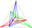
(b)

Figure 2: (a) The crossed dodecahedron graph, which does not admit a straight-line 2-planar drawing and (b) $K_{9}$, which has rectilinear thickness three. Dotted edges are uncrossed and can be colored arbitrarily.

A set of $k+\ell$ edges of a graph is said to form a $(k,\ell)$-grid [25, 26] if each of the first $k$ edges crosses all of the remaining $\ell$ edges, see Fig. 3. A $(k,\ell)$-grid is radial if, in addition, the first $k$ edges are incident to the same vertex, that is they form a fan, and natural if all $k+\ell$ edges are independent. Hence, a graph is $k$-planar, fan-crossing and fan-crossing free, respectively, if and only if it avoids $(k+1,1)$, natural $(2,1)$ and radial $(2,1)$-grids, respectively. We call a graph tri-fan-crossing if it admits a drawing so that each edge is crossed by edges of a fan if the edge is crossed at least three times.

(a)

(b)

(c)

(d)

Figure 3: (a) A radial $(3,1)$-grid or a fan-crossing, (b) a natural $(3,1)$-grid and a fan-crossing free drawing, (c) a $(3,1)$-grid, and (d) three pairwise crossing edges.

The thickness of a graph [27] is the minimum number of planar graphs into which the edges can be partitioned. Thickness has received much attention [28]. It has applications in VLSI design [29], where crossed edges must be embedded in different layers, and in graph visualization, where there is an edge coloring so that edges of the same color do not cross. The thickness of a graph is bounded by its arboricity, which is the minimum number of forests into which a graph can be decomposed. The arboricity of a graph is the maximum density of any subgraph, that is $\max\{\lceil\frac{|E[U]|}{|U|-1}\rceil\}$, where $U$ is a subset of vertices and $E[U]$ is the set of edges with both vertices in $U$ [30]. It can be computed in $O(n^{3/2})$ time if graphs have $O(n)$ many edges [31]. One third of the arboricity is a lower bound for the thickness.

The rectilinear thickness of a graph G, also known as real linear thickness [32] or geometric thickness [33], is the minimum number of colors in a straight-line drawing of $G$, so that edges of the same color do not cross. It is a real restriction, since complete graphs have thickness $\lfloor(n+7)/6\rfloor$ for $n\neq 9,10$ [34], whereas they have geometric thickness at least $\lceil(n+1)/5.646\rceil$ [35]. Moreover, Eppstein [33] showed that for every $k$, there are graphs with thickness three and rectilinear thickness at least $k$. Hence, geometric thickness is not bounded by thickness.

Graphs with thickness two, also called biplanar graphs [36], were studied by Hutchinson et al. [37]. They showed that graphs with rectilinear thickness two have at most $6n-18$ edges, and that the complete graph $K_{8}$ is the largest complete graph with rectilinear thickness two, since $K_{9}$ and $K_{10}$ have thickness three [34]. Note that $K_{9}$ has rectilinear thickness three, as shown in Fig. 2(b).

Geometric thickness specializes to book thickness if all vertices are placed in convex position. It is known that planar graphs have book thickness four [38], where the lower bound was proved just recently [39, 40], and that the book thickness of 1-planar graphs is bounded by a constant [41].

In the remainder of this work, we introduce basic notions in Section 2 and recall methods for straight-line drawings of planar graphs. In Section 3, we first show that every 3-connected 1-planar graph admits a straight-line biplanar grid drawing. Such drawings scaled down for the general case so that they fit into the first inner face.

2 Preliminaries

We consider simple undirected graphs with $n$ vertices and colored edges and assume that graphs are biconnected and are given with a drawing (or a simple topological embedding) in the plane. For convenience, we do not distinguish between a graph and its 1-planar drawing, a vertex, its point in a drawing, and its position in a canonical ordering, and an edge and its line in a drawing. We also refer to a leftmost lower neighbor or a lower (left) subgraph if this is clear from the drawing of a planar graph.

Straight-line grid drawings of planar graphs can be constructed by using the canonical ordering and the shift method, introduced by de Fraysseix et al. [9]. Alternatively, Schnyder realizers can be used [10]. A canonical ordering of a triconnected planar graph $G$ is a bucket order $V_{1},\ldots,V_{m}$ of its vertices, so that further properties are satisfied [13]. A bucket $V_{i}$ consists of a single vertex or a set of vertices forming a path that is a part of the boundary of a face of a planar drawing of $G$. The first bucket consists of two vertices $v_{1}$ and $v_{2}$ in the outer face, called the base. The last bucket consists of another vertex in the outer face. Let $G_{k}$ denote the subgraph induced by the vertices from the first $k$ buckets. Its outer face, called contour, contains $v_{1},v_{2}$ and the vertices of $V_{i}$. Every $G_{k}$ is biconnected and internally triconnected, so that separation pairs are on the contour.

A canonical ordering of a triconnected planar graph can be computed in linear time [13]. In general, a planar graph has many canonical orderings, for example a leftmost and a rightmost one [13]. In particular, if the base is fixed, then any other vertex in the outer face can be chosen as the last vertex. If the last vertex $t_{1}$ is in a separating triangle $(t_{1},t_{2},t_{3})$, then there are canonical orderings $t_{2}<t_{3}<w<t_{1}$ and $t_{3}<t_{2}<w<t_{1}$, where vertex $w$ is in the interior of $(t_{1},t_{2},t_{3})$, since there is a canonical ordering of a subgraph with $t_{1}$ and the vertices in the interior of $(t_{1},t_{2},t_{3})$ removed and with $t_{2}$ or $t_{3}$ as last vertex. The vertices in the interior of $(t_{1},t_{2},t_{3})$ follow $t_{2}$ and $t_{3}$ by biconnectivity.

The drawing of a graph in the plane is 1-planar if each edge is crossed at most once. Then edges cross in pairs. The crossing point partitions a crossed edge into two uncrossed segments, whereas an uncrossed edge consists of a single segment. A graph $G$ is 1-planar if it admits a 1-planar drawing. A 1-planar drawing is planar-maximal if no uncrossed edge can be added without violating 1-planarity. This property is assumed from now on. Alternatively, one may consider maximal 1-planar drawings, which do not admit the addition of any edge without violation. The planar skeleton is obtained by removing all pairs of crossed edges. For an algorithmic treatment, we use the planarization, which is obtained from a 1-planar drawing by treating each crossing point as a special vertex of degree four [15]. Clearly, a 1-planar drawing can be augmented to a planar-maximal one in linear time.

A separation pair $\langle u,v\rangle$ partitions a graph into components, so that $G-\{u,v\}=H_{0}^{-},\ldots,H_{r}^{-}$ for some $r\geq 1$. Let $H_{i}$ denote the subgraph induced by the vertices of $H_{i}^{-}$ and the vertices from the separation pair, so that the common edge $(u,v)$ is in the outer face. The (edges between $u$ and vertices of the) components $H_{0},\ldots,H_{k}$ are ordered clockwise at $u$ and counter clockwise at $v$. Two consecutive components are separated by one or two pairs of crossed edges if $G$ is planar-maximal 1-planar. The outer component $H_{0}$ contains vertices in the outer face if all crossed edges are removed. All other components are called inner components. Every inner component $H_{i}$ has a first inner face, which is the face next to edge $(u,v)$ in the subgraph induced by $H_{0},\ldots,H_{i}$, that is the later inner components $H_{i+1},\ldots H_{r}$ are removed.

There is a B- or a W-configuration if a pair of edges crosses in the outer face of a component [14]. Alam et al. [42] observed that B-configurations can be avoided if the embedding is changed by a flip, see Figs. 1(b) and 1(c). A W-configuration consists of six vertices $v_{1},v_{2},u_{1},u_{2},t_{1},t_{2}$, so that there are two pairs of crossed edges $(v_{1},u_{2})$, $(v_{2},u_{1})$ and $(v_{1},t_{2})$, $(v_{2},t_{1})$, see Fig. 1(a). Vertices $v_{1}$ and $v_{2}$ are the base with edge $(u,v)$ uncrossed and vertices $t_{1}$ and $t_{2}$ are on top. By a flip, the pairs $(t_{1},t_{2})$ and $(u_{1},u_{2})$ can be exchanged, so that $u_{1}$ and $u_{2}$ are on top in another embedding.

The drawing of an edge-colored 1-planar graph is called specialized if there are vertices $v_{1},v_{2},t_{1}$ and $t_{2}$, so that the outer face is an isosceles triangle $(v_{1},v_{2},t_{2})$ and edges incident to $v_{2}$ are black. Moreover, the drawing is 1-planar, except for edge $(v_{1},t_{1})$, which is crossed by edges incident to $t_{2}$ and edges crossing $(v_{1},t_{1})$ are crossed at most twice.

Hence, a specialized drawing is tri-fan-crossing. It is 1-planar if either edge $(v_{1},t_{1})$ or vertex $t_{2}$ is removed, see Figs. 5(b) and 6(c).

Alam et al. [42] have shown that every triconnected 1-planar graph can be drawn straight line on a grid of quadratic size, except, possibly, for one edge in the outer face. They use the algorithm by Chroback and Kant [12] for a drawing of the planar skeleton, whereas we prefer the one by Kant [13], which creates edges with slope $-1,0$ and $+1$ on the contour.

Lemma 1

A triconnected 1-planar graph $G$ admits a straight-line 1-planar drawing if and only if $G$ has at most $4n-9$ edges. If existing, there is a specialized drawing on a grid of size at most $(4n-8)\times(2n-4)$, so that the outer face is an isosceles right-angled triangle. An edge is uncrossed in the straight-line drawing if and only if it is uncrossed in (the 1-planar drawing of) $G$. Its length $\ell$ is bounded by $1\leq\ell\leq 4n-8$.

Proof

Form [43, 44] and [16] we obtain that a 1-planar drawing of a planar-maximal 1-planar graph $G$ has a triangular face with three uncrossed edges if and only if $G$ has at most $4n-9$ edges. Choose this triangle as the outer face. As shown by Kant [13], there is a convex drawing of the planar skeleton on a grid of size at most $(2n-4)\times(n-2)$, so that the outer face is an isosceles right-angled triangle. The drawing can be turned into a strictly convex drawing on a grid of size at most $(4n-8)\times(2n-4)$ if two extra shifts are used for any two edges of a quadrangle that are in a line, as shown in [42, 45]. See Fig. 4 for an illustration. Every pair of crossed edges is reinserted into the quadrangle from which it was removed. Uncrossed edges are colored black. There is a black and a red edge if two edges cross, where the coloring is chosen so that all edges incident to vertex $v_{2}$ are black. Then the drawing is specialized. At its creation, an uncrossed edge has length at least one, since there is a grid drawing. Later on, edges are stretched by horizontal shifts. The base is the longest edge and is a horizontal line of length at most $4n-8$.

(a)

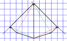
(b)

Figure 4: Placement of vertex $v$ (a) in general and (b) for strict convexity.

3 Straight-line Biplanar Drawings of 1-Planar Graphs

It is clear that every 1-planar graph is biplanar. In fact, every 1-planar graph can be decomposed into a planar graph and a forest [46]. Towards a straight-line biplanar drawing, we first consider triconnected 1-planar graphs with a pair of edges crossing in the outer face. These edges must be redrawn. We show that there is a straight-line biplanar grid drawing, which is 1-planar with the exception of edges incident to the top vertices of a W-configuration. In general, there is a separation pair if there is a pair of crossed edges in the outer face of a component. By induction, every inner component at a separation pair has a straight-line biplanar drawing, which is scaled down, so that it fits into the first inner face of the outer component. So we obtain a biplanar drawing of a 1-planar graph. By upper and lower bounds on the length of (segments of) edges, we can estimate that a single inner component is scaled down at most by $c/n^{5}$ for some $c>0$. In return, the outer component is scaled up by $O(n^{5})$. By induction on the number of inner components and recursion on separation pairs, the upscaling is bounded by $O(n^{n})$, so that we use high precision arithmetic with numbers with $O(n\log n)$ many digits.

Lemma 2

Let $G$ be a 3-connected 1-planar graph with a W-configuration in the outer face, so that the vertices $v_{1}$ and $v_{2}$ from the base are the first and the vertices $t_{1}$ and $t_{2}$ on top are the last two vertices in a canonical ordering of the planar skeleton of $G$. Then $G$ admits a specialized straight-line biplanar drawing $\Gamma(G)$ on a grid of quadratic size. A segment of an edge $e$ has length $\ell$ with $1\leq\ell\leq 8n-16$ in $\Gamma(G)$ if $e$ is uncrossed in (the 1-planar drawing of) $G$.

Proof

The outer face of the planar skeleton of $G$ is a quadrangle with vertices $v_{1},v_{2},t_{1}$ and $t_{2}$ from the W-configuration. Let $t_{2}$ be the last vertex and assume that there is no inner quadrangle containing $v_{2}$ and $t_{2}$. Otherwise, let $t_{1}$ be the last vertex. The canonical ordering is $\{v_{1},v_{2}\}<v<t_{1}<t_{2}$ for any other vertex $v$. A bucket consists of one or two vertices, since the faces of the planar skeleton are triangles or quadrangles. There is a quadrangle if and only if it contains a pair of crossed edges in the 1-planar drawing of $G$.

Our algorithm uses the shift method and incrementally adds a vertex or the pair of vertices with a horizontal edge in between to an intermediate drawing. Similar to Alam et al. [42], we extend the algorithms by de Fraysseix et al. [9] and Kant [13], so that there are strictly convex inner faces for a planar drawing of the planar skeleton. Our algorithm is based on the algorithm for 3-connected planar graphs by Kant [13], which constructs a drawing with convex inner faces on a grid of size $(2n-4)\times(n-2)$. Strict convexity for inner quadrangles is obtained by extra shifts, so that there is a straight-line planar drawing of the planar skeleton on a grid of size at most $(4n-8)\times(2n-4)$ [42, 45], see Fig. 4.

In detail, we construct the biplanar drawing $\Gamma(G)$ as follows. The planar subgraph of $G-\{t_{1},t_{2}\}$ is drawn as described before with a horizontal line for $(v_{1},v_{2})$. All quadrangles containing $t_{2}$ are prepared for strict convexity, so that edges $(a,b)$ and $(b,c)$ are not in a line for a quadrangle $(a,b,c,t_{2})$. Crossed edges are inserted in the interior of the quadrangle from which they were removed if they are not incident to $t_{1}$ or $t_{2}$. By Lemma 1, the intermediate drawing is straight-line and 1-planar on a grid of size at most $(4n-16)\times(2n-8)$. The uncrossed edges have length at least one and at most $4n-16$.

By the restrictions for a canonical ordering [13], the last two vertices are placed one after another. First, add $t_{1}$ and its incident edges to lower vertices including the crossed edge $(t_{1},v_{1})$, so that there is an isosceles right-angled triangle $(v_{1},v_{2},t_{1})$ with $t_{1}$ on top. Edge $(t_{1},v_{1})$ is colored red, so that it is transparent for black edges incident to $t_{2}$, see Fig. 5(a). The lower neighbors of $t_{2}$ are on the contour of the drawing of $G-t_{2}$ if edge $(t_{1},v_{1})$ is ignored. Let $v$ be the rightmost lower neighbor of $t_{2}$ so that $v\neq v_{2}$. If $v$ is $x\geq 0$ units to the right of $t_{1}$, then shift $v_{2}$ by $2x+2$ extra units to the right and place $t_{1}$ at the intersection of the diagonals through $v_{1}$ and $v_{2}$, so that it moves by $(x+1,x+1)$ from its former position. Clearly, $2x+2\leq 4n-8$. Thereafter, all neighbors of $t_{2}$ are to the left of $t_{1}$, except for $v_{2}$, which is the rightmost vertex. At last, shift $v_{1}$ one unit to the left and $v_{2}$ one unit to the right and place $t_{2}$ at the intersection of the diagonals, so that $t_{2}$ is one unit vertically above $t_{1}$, and draw all edges incident to $t_{2}$ straight line, see Fig. 5(b).

All uncrossed edges of $G$ are colored black. Edge $(t_{1},v_{1})$ is colored red. The edges incident to $t_{2}$ and $v_{2}$ are colored black, so that all edges crossing an edge incident to $t_{2}$ or $v_{2}$ in the interior of a quadrangle are colored red. Recall that there is no inner quadrangle with $t_{2}$ and $v_{2}$. For all other pairs of crossed edges in a quadrangle choose any coloring, so that one crossed edge is red and the other is black.

By Lemma 1 and the placement of $t_{1}$, the drawing of $G-t_{2}$ is straight-line 1-planar. The red edge $(t_{1},v_{1})$ is the leftmost edge when $t_{1}$ is placed, so that it does not cross any red edge. Hence, red edges do not cross, since edges incident to $t_{2}$ are black and other red edges are in the interior of strictly convex quadrangles. Black edges do not cross if they are not incident to $t_{2}$ by Lemma 1. Edges $(t_{2},v_{1})$ and $(t_{2},v_{2})$ are in the outer face and are uncrossed. Any other edge incident to $t_{2}$ is crossed by the red edge $(t_{1},v_{1})$, which is not crossed by other edges, so that $(t_{1},v_{1})$ is crossed by edges of a fan at $t_{2}$. Edge $(t_{2},v)$ is crossed by an edge $(u,u^{\prime})\neq(t_{1},v_{1})$ in $\Gamma(G)$ if and only if edges $(t_{2},v)$ and $(u,u^{\prime})$ cross in the 1-planar drawing of $G$. Then $(u,u^{\prime})$ is colored red and there is a strictly convex quadrangle $(t_{2},u,v,u^{\prime})$ in $\Gamma(G)$. Edge $(t_{2},v)$ is not crossed by any further edge, so that it is crossed at most twice. Hence, $\Gamma(G)$ is a specialized straight-line biplanar grid drawing.

The grid has size at most $(8n-16)\times(4n-8)$, since the size of at most $(4n-8)\times(2n-4)$ by Lemma 1 is extended by at most $4n-8$ additional shifts for vertex $t_{2}$. Clearly, edge $(v_{1},v_{2})$ is the longest edge in $\Gamma(G)$ with a length bounded by $8n-16$. Uncrossed edges of $G$, that is edges of the planar skeleton, are uncrossed in $\Gamma(G)$ if they are not incident to $t_{2}$, and uncrossed edges incident to $t_{2}$ are only crossed by $(t_{1},v_{1})$ in $\Gamma(G)$. An uncrossed edge has length at least one by Lemma 1. If $(t_{2},v)$ is uncrossed in $G$, then it has two segments from $t_{2}$ to the crossing point with $(t_{1},v_{1})$ and from there to $v$, see Fig. 5(c). The first segment has length greater than one, since $t_{2}$ is placed one unit above $t_{1}$, and the second segment has length $\ell>1$, since $v$ is at least two units below $t_{1}$ and $(t_{1},v_{1})$ has slope $(h-1)/h$, where $h$ is the height (or half of the width) of the drawing. Hence, segments of uncrossed edges of $G$ have length at least one, whereas segments of crossed edges can be very short.

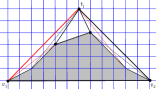
(a)

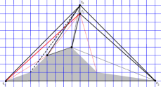
(b)

(c)

Figure 5: Illustration to the proof of Lemma 2. (a) The drawing up to vertex $t_{1}$. (b) Extra shifts for $t_{1}$, the insertion of $t_{2}$ and an edge coloring, and (c) the length of segments of edges crossed by $(t_{1},v_{1})$.

We now consider a W-configuration with last vertex $t_{1}$, so that the second top vertex $t_{2}$ cannot be the last but one vertex in the canonical ordering. Then there are separating triangles with vertices $t_{1}$ and $t_{2}$. We can assume that a flip of the component at the base, as in Figs. 1(b) and 1(c), does not help to avoid a separating triangle with the top vertices. Otherwise, Lemma 1 or Lemma 2 are used for the changed embedding.

Lemma 3

Every 3-connected 1-planar graph $G$ with a pair of crossed edges in the outer face admits a specialized straight-line biplanar drawing $\Gamma(G)$ on a grid of size $O(n^{7})$. In addition, the outer face is an isosceles obtuse angled triangle, and a segment of edge $e$ in $\Gamma(G)$ has length $\ell$ with $1\leq\ell\leq cn^{5}$ for some $c>0$ if $e$ is uncrossed in (the 1-planar drawing of) $G$.

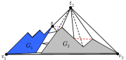
(a)

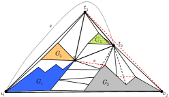
(b)

(c)

Figure 6: Illustration to the proof of Lemma 3. (a) A 1-planar drawing of $G$ up to vertex $t_{2}$, and (b) a 1-planar drawing of $G^{-}$, in which edge $e=(v_{1},t_{2})$, drawn black and dotted, is missing. Crossed edges are drawn dashed. (c) A biplanar drawing of $G$, which is obtained from the 1-planar drawing by moving $t_{2}$ along edge $(s,t_{2})$ above $t_{1}$ and shifting $G_{2}$.

Proof

Consider a canonical ordering $v_{1},v_{2},\ldots,t_{1}$ of the planar skeleton of $G$, so that there is a W-configuration with base $v_{1},v_{2}$ and top vertices $t_{1}$ and $t_{2}$ in $G$ with $v_{1}$ left of $v_{2}$. There is a separating triangle $(s,t_{1},t_{2})$ if $t_{2}$ cannot be the last but one vertex in a canonical ordering. Choose $s$ so that $(s,t_{1},t_{2})$ is maximal in the sense that its vertices are not contained in another separating triangle with vertices $t_{1}$ and $t_{2}$. In other words, $s$ is the least vertex in a separating triangle with $t_{1}$ and $t_{2}$. Vertices $s$ and $t_{2}$ are in the outer face of the planar skeleton of $G-t_{1}$. Since there is a W-configuration, we have $s\neq v_{1}$ and $s\neq v_{2}$. Assume $s<t_{2}$ in the canonical ordering. If this order is impossible, then there is a separating triangle $(s^{\prime},t_{1},t_{2})$ containing $s$, so that $(s,t_{1},t_{2})$ is not maximal and $s$ is not the least such vertex, contradicting our assumption. Vertex $s$ is the leftmost lower neighbor of $t_{2}$, so that $t_{2}$ is first placed at the intersection of the diagonals through $s$ and $v_{2}$, as shown in Fig. 6(a).

Let $G^{-}$ be the subgraph of $G$ without the crossed edge $e=(v_{1},t_{2})$, drawn black and dotted in Fig. 6(b). Graph $G^{-}$ decomposes into four subgraphs. Subgraph $G_{4}$ consist of the vertices in the interior of the separating triangle $(s,t_{1},t_{2})$ including $s,t_{1}$ and $t_{2}$, so that $s<t_{2}<v<t_{1}$ for every vertex $v$ in the separating triangle. Subgraph $G_{3}$ is induced by the vertices $v>s$ and $v\not\in G_{4}$. Subgraph $G_{2}$ consists of the vertices $v<s$ under $t_{2}$, as described in [12, 47, 48, 9, 13], and $G_{1}$ is the remainder with vertices $v<s$. If $s$ is to the left of $t_{2}$, then $G_{1}$ is to the left of $G_{2}$ and $G_{3}$ is to the left of $G_{4}$. By the shift method, the vertices of $G_{2}$ are shifted horizontally with $t_{2}$.

We first construct a 1-planar drawing of $G^{-}$ as described in Lemma 1, with the following modifications for horizontal edges in $G_{4}$ and vertex $t_{2}$. Vertex $t_{2}$ is first placed at the intersection of the diagonals through $s$ and $v_{2}$, so that it is $h\geq 1$ units above $s$. Every vertex $v$ of $G_{4}$ with $t_{2}<v<t_{1}$ is placed above the line $(s,t_{2})$, using the shift method as described in Lemma 1, with the following exception. If there is a bucket in the canonical ordering with vertices $y$ and $z$, so that $t_{2}$ is the rightmost lower neighbor of $z$, then there is a quadrangle $(x,y,z,t_{2})$ in the planar skeleton, so that $x$ is the leftmost lower neighbor of $y$ and $(y,t_{2})$ is crossed by $(x,z)$ in $G$. The previous algorithm [13] draws edge $(y,z)$ as a horizontal line of length two. We draw it with slope $h/(h+2)$, so that $(x,y,z,t_{2})$ is a strictly convex quadrangle. This is achieved by $2h$ extra shifts for $t_{2}$, so that $y$ is placed at $(h,h)$ from its former position. Edges $(x,y)$ and $(t_{2},z)$ have slope +1 and -1, respectively, when $y$ and $z$ are placed. The slope of $(x,t_{2})$ is negative if $x\neq s$, since $x$ is placed after $t_{2}$ in this case. If there is a quadrangle $(s,y,z,t_{2})$ just above $(s,t_{2})$, then edge $(s,t_{2})$ has slope $h/(3h+4)$ at the placement of $y$ and $z$, which is less than the slope of $h/(h+2)$ for $(y,z)$. Later on, edges are flattened by the shift method, which reduces the angular resolution, whereas a positive angle between adjacent adjacent edges is preserved. If there is a triangle $(a,b,t_{2})$ in the 1-planar drawing of $G_{1}$, then $t_{2}$ is the rightmost lower neighbor of $b$, so that $(t_{2},b)$ has slope -1 when $b$ is placed. The slope of $(a,b)$ is at least one if it is positive. It may be negative.

Since only techniques from the shift method [9, 13] are used, there is a straight-line strictly convex drawing of the planar skeleton of $G$ (or $G^{-}$) on a grid of size at most $h(4n-8)\times h(2n-4)$, where $h$ is the vertical distance between $s$ and $t_{2}$. In this drawing, edge $(s,t_{2})$ has slope $\alpha$ with $\frac{h}{4hn_{4}}\leq\alpha<1$, where $n_{4}$ is the number of vertices of $G_{4}$ in the interior of the triangle $(s,t_{1},t_{2})$, since $t_{2}$ is shifted horizontally at most $4h$ units per vertex of $G_{4}$ according to Lemma 1. The height $h$ is bounded by $1\leq h\leq 2n_{2}-4$, since only vertices of $G_{2}$ shift $v_{2}$ relative to $s$, where $n_{2}$ is the set of vertices of $G_{2}$. The length of an uncrossed edge is at least one and at most $h(4n-8)<8n^{2}$. The crossed edges are inserted into the quadrangles from which they were removed, so that there is a 1-planar drawing of $G^{-}$.

This drawing is modified by moving $t_{2}$ above $t_{1}$, so that the missing edge $(v_{1},t_{2})$ can be added for a specialized straight-line biplanar drawing $\Gamma(G)$. Note that $t_{2}$ has further neighbors only in $G_{2}$ and $G_{4}$, since $(s,t_{1},t_{2})$ is a separating triangle and $s$ is the leftmost lower neighbor of $t_{2}$. Extend edge $(s,t_{2})$ until it crosses the horizontal line two units above $t_{1}$, and move $t_{2}$ to the grid point at or next right of the crossing point. Thereby, $t_{2}$ is moved $x_{2}$ units to the right and $y_{2}$ units upward. Edge $(s,t_{2})$ is flattened, since $y_{2}/x_{2}\leq\alpha\leq y_{2}/(x_{2}-1)$. By the shift method, the vertices of $G_{2}$ are shifted horizontally with $t_{2}$, that is $x_{2}$ units to the right. Next, reroute edge $(t_{2},v_{1})$ from $t_{2}$ through the grid point one above $t_{1}$ until it crosses the x-axis, that is the horizontal line through $v_{1}$ and $v_{2}$, and shift $v_{1}$ to the grid point at or just left of the crossing point. Edge $(t_{1},v_{2})$ is rerouted and is drawn along a ray through the grid point one unit above $G_{2}$, which is obtained by the tangent from $t_{1}$ to the convex hull of the drawing of $G_{2}$. Then $v_{2}$ is shifted horizontally to the grid point at or next right of the crossing point of the ray and the x-axis, see Fig. 6(c). Finally, shift $v_{1}$ or $v_{2}$ horizontally so that there is an isosceles triangle with top $t_{2}$.

Edge $(t_{1},v_{2})$ is colored red. Edges incident to $t_{2}$ are colored black, and their crossing edges are colored red. All uncrossed edges and all crossed edges incident to $v_{1}$ are colored black, whereas the coloring of the remaining pairs of crossed edges can be chosen arbitrarily. This completes the construction of $\Gamma(G)$.

We claim that $\Gamma(G)$ is a specialized straight-line biplanar grid drawing. Since there is a straight-line 1-planar grid drawing for $G^{-}$, it suffices to consider the modifications for $\Gamma(G)$. By construction, all edges are drawn straight line and all vertices are placed on grid points. Red edges do not cross, since they do not cross in the 1-planar drawing of $G^{-}$ and $(t_{1},v_{2})$ crosses only edges incident to $t_{2}$, which are black. Such an edge may be crossed by a red edge in the interior of a convex quadrangle. Two black edges do not cross if none of them is incident to $t_{2}$, since they are drawn as in $\Gamma(G^{-})$, or a vertex of the edge (or both) is shifted horizontally if a vertex is in $G_{2}$. Recall that horizontal shifts preserve planarity and convexity, as observed at several places [12, 9, 13]. Clearly, two edges incident to $t_{2}$ do not cross, since the edges are not drawn on top of one another. It remains to consider a black edge incident to $t_{2}$ and black edges of $G_{2}$ and $G_{4}$, see Fig. 6.

Vertex $t_{2}$ and the vertices of $G_{2}$ are shifted $x_{2}$ units to the right, and then $t_{2}$ is shifted $y_{2}$ units upward to its final position. As observed by de Fraysseix et al. [9], such shifts do not create crossings, and they preserve strict convexity. In particular, a strict convexity of a quadrangle $(t_{2},s,u,u^{\prime})$ with vertices $u,u^{\prime}\in G_{2}$ is preserved, so that the crossed edge $(t_{2},u)$ is drawn straight-line in $\Gamma(G)$ and is crossed by the red edge $(s,u^{\prime})$. Hence, edges $(t_{2},v)$ and $(u,u^{\prime})$ with $u\in G_{2}$ cross in $\Gamma(G)$ if and only if they cross in in the 1-planar drawing of $G^{-}$.

At last consider edges $(v,t_{2})$ with $v\in G_{4}$ in the 1-planar drawing of $G^{-}$. Vertex $v$ is placed above $t_{2}$ in $\Gamma(G^{-})$, but it is below $t_{2}$ in $\Gamma(G)$ after moving $t_{2}$, so that the slope of $(v,t_{2})$ changes from negative to positive, see Fig. 6. We claim that moving $t_{2}$ does not create new crossings with edges in $G_{4}$, since $(s,t_{2})$ is flat and horizontal edges in quadrangles with $t_{2}$ are lifted. Consider the drawing of $G_{4}$ without vertex $t_{2}$, which is obtained from the 1-planar drawing of $G^{-}$ by removing $t_{2}$. The part of the outer face of $\Gamma(G-t_{2})$ and $\Gamma(G^{-}-t_{2})$ between $s$ and $t_{1}$ consists of the neighbors $u_{0},\ldots,u_{r}$ of $t_{2}$ in clockwise order, so that $s=u_{0}$ and $t_{1}=u_{r}$. These vertices are ordered in the canonical ordering, so that $u_{i}$ is placed after $u_{i-1}$. There are three cases: (1) $u_{i-1}$ is the leftmost lower neighbor of $u_{i}$, (2) there is a quadrangle with vertices $u_{i-2},u_{i-1},u_{i}$ and $t_{2}$, so that $(u_{i-1},t_{2})$ is crossed by $(u_{i-2},u_{i})$ or (3) $u_{i-1}$ is in the under-set of $u_{i}$. In case (1), $u_{i}$ is placed on the +1 diagonal through $u_{i-1}$, so that $(u_{i-1},u_{i})$ has slope +1 when it is created. In case (2), edge $(u_{i-1},u_{i})$ is lifted and is not drawn as a horizontal line, as in [13]. Edge $(u_{i},u_{i-2})$ is red, since its crossing edge is incident to $t_{2}$. Edge $(u_{i-2},u_{i-1})$ has slope +1 and $(u_{i-1},u_{i})$ has slope $h/(h+2)$ when $u_{i-1}$ and $u_{i}$ are placed. At this moment, edge $(s,t_{2})$ has slope $h/W_{i}$ so that $W_{i}>h+2$. In case (3), vertex $u_{i-1}$ is in the under-set of $u_{i}$, so that (the slope of) edge $(u_{i-1},u_{i})$ is fixed, and is only shifted from now on. Its slope is greater than one or may be negative, which is even simpler, since $u_{i-1}$ is visible from $t_{2}$ in $\Gamma(G)$ in the sense that there is an unobstructed (uncrossed) line of sight between $u_{i-1}$ and $t_{2}$ if the red edge $(t_{1},v_{2})$ is ignored.

Consider case (2) for the drawing of $G^{-}$. Cases (1) and (3) are similar. Edge $(u_{i-1},u_{i})$ has slope $h/w_{i}$ and edge $(s,t_{2})$ has slope $h/W_{i}$ with $w_{i}<W_{i}$, when edge and $(u_{i-1},u_{i})$ is drawn first. Edge $(u_{i-1},u_{i})$ is flattened if vertices are placed above it, so that $u_{i-1}$ and $u_{i}$ are shifted apart. Vertex $t_{2}$ is shifted by the same quantity. Hence, the slope of $(s,t_{2})$ remains less than the slope of $(u_{i-1},u_{i})$, since $h/w_{i}<h/W_{i}$ implies $h/(w_{i}+x)<h/(W_{i}+x)$ if there is a horizontal shift by $x$ units. In other words, edge $(s,t_{2})$ in $\Gamma(G)$ is flatter that any edge $(u_{i-1},u_{i})$ for with $1\leq i<r$. By induction, edge $(u_{i},t_{2})$ with $1\leq i<r$ is uncrossed in $\Gamma(G)$ if the red edges $(t_{1},v_{2})$ and $(u_{i-1},u_{i+1})$ in quadrangles $(u_{i-1},u_{i},u_{i+1},t_{2})$ are ignored. In other words, moving $t_{2}$ in direction of $(s,t_{2})$ preserves the visibility of its neighbors in $G_{4}$. Hence, the obtained drawing $\Gamma(G)$ is biplanar. In addition, the edges incident to $v_{1}$ are black, edge $(t_{1},v_{2})$ is crossed by edges of a fan at $t_{2}$, and edges incident to $t_{2}$ are crossed twice if they are crossed in the 1-planar drawing of $G^{-}$. Hence, the drawing is specialized.

Consider the size of the drawing. The 1-planar drawing of $G^{-}$ has size at most $h(4n-8)\times h(2n-4)$, where $h\leq 2n-4$ is the difference between $s$ and $t_{2}$ in y-dimension. Edge $(s,t_{2})$ has slope at least $1/4n$. Vertex $t_{1}$ is at most $h(2n-4)$ units above $t_{2}$. Hence, $t_{2}$ is shifted at most $16n^{3}$ units to the right. The ray from $t_{2}$ along $t_{1}$ crosses the x-axis at most $128n^{5}$ units to the left of $v_{1}$, since its slope is at least $1/16n^{3}$ and $t_{1}$ is at height at most $8n^{2}$. Similarly, the ray from $t_{1}$ along the top of $G_{3}$ to $v_{2}$ crosses the x-axis at most $32n^{4}$ units to the right of $t_{1}$. Hence, the width of the drawing is $O(n^{5})$, and the height is $O(n^{2})$.

The upper bound on the length of an edge is $O(n^{5})$. The lower bound is one for an uncrossed edge, since there is a grid drawing. An uncrossed edge of $G$ is crossed in $\Gamma(G)$ if it is incident to $t_{2}$ and is crossed by $(t_{1},v_{2})$, see Fig. 6(c). The first segment from $t_{2}$ has length at least two, since $t_{2}$ is two units above $t_{1}$ and the slope of $(t_{1},v_{2})$ is negative. The crossing point of $(t_{1},v_{2})$ and $(t_{2},v)$ for a vertex in $G_{2}$ or $G_{4}$ is at least one unit above $v$, where $t_{1}$ is placed at least two units above the vertices of $G_{4}$ in the drawing of $G^{-}$, so that the second segment of $(t_{2},v)$ has length at least one.

If $\langle u,v\rangle$ is a separation pair with components $H_{0},\ldots,H_{r}$, then $(u,v)$ is an uncrossed edge if the graph is planar-maximal 1-planar or it can be rerouted so that it is uncrossed, see Fig. 7. There is a first inner face next to $(u,v)$ for $H_{i}$ if the inner components $H_{j}$ with $j>i\geq 0$ are removed. Hence, $H_{i+1},\ldots,H_{r}$ are drawn in the interior of the first inner face for $H_{i}$. This face is a triangle whose third vertex is a crossing point or the first vertex of $H_{i}^{-}$. In a biplanar drawing, the triangle can be intersected by a red edge from a previous component, for example if $v$ is the top of the outer triangle, as stated in Lemmas 2 and 3 and illustrated in Figs. 5(b) and 6(c). Since the last vertex can be chosen among the two top vertices of a W-configuration, for every inner component $H_{i}$, there is a specialized biplanar drawing so that the edges incident to $v$ are black.

(a)

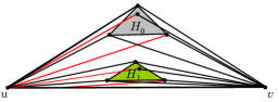
(b)

Figure 7: (a) A 1-planar drawing with W-configurations for the outer component $H_{0}$ and inner component $H_{1}$. (b) A biplanar drawing with $H_{1}$ drawn in the first inner face of $H_{0}$. Note that quadrangles in the outer face of the planar skeleton of a 1-planar drawing are turned into a triangles in the biplanar drawing. Drawing (b) is scaled down.

The vertices of an uncrossed edge are a candidate for a separation pair. In fact, there is a 1-planar drawing if every uncrossed edge $e$ of a 1-planar drawing is substituted by a 1-planar graph $G_{e}$, so that $e$ is uncrossed in $G_{e}$. For example, edge $e$ can be substituted by $K_{6}$, drawn as a W-configuration. In general, this property does not hold for the vertices of a crossed edge, since the addition of a component violates 1-planarity or the edge is uncrossed in another drawing.

Lemma 4

A 1-planar graph admits a specialized straight-line biplanar drawing if it has a single separation pair with an inner and an outer component. The drawing of the outer component is scaled by $O(n^{5})$ and segments of uncrossed edges have length at least one.

Proof

Suppose that $\langle u,v\rangle$ is a separation pair so that $G-\{u,v\}$ partitions into an outer component $H_{0}$ and an inner component $H_{1}$. Edge $(u,v)$ is uncrossed in a 1-planar drawing of $G$. It is the uncrossed base of $H_{1}$. It is uncrossed in a specialized straight-line biplanar drawing of $H_{0}$ if $u$ and $v$ are not part of a W-configuration of $H_{0}$ by Lemma 1. Otherwise, there is a red edge that crosses black edges incident to $v$ by Lemmas 2 and 3, see Fig. 8(a).

Independently, compute specialized straight-line biplanar drawings $\Gamma(H_{0})$ and $\Gamma(H_{1})$, which each include edge $(u,v)$. Let $w_{1}$ and $h_{1}$ be the width and the height of $\Gamma(H_{1})$, so that $(u,v)$ is a horizontal line of length $w_{1}$. In the drawing of $H_{0}$ it is a line of length $w_{0}$ with slope $\alpha$. The first inner face of $\Gamma(H_{0})$ next to $(u,v)$ is a triangle with height $h_{0}$. By Lemmas 2 and  3, the width and height of $\Gamma(H_{0})$ and $\Gamma(H_{1})$ is at most $128n^{5}$ and $2n^{2}$, respectively, and the first inner face has height $h\geq 1/(256n^{5})$, since it is a triangle $(v_{1},v_{2},p)$, where $(v_{1},v_{2})$ is a horizontal line of length at most $128n^{5}$ and $p$ is the third vertex one unit above $(u,v)$ or the crossing point of edges with slope at least $1/(128n^{5})$.

Scale $\Gamma(H_{1})$ in x-dimension by $w_{0}/w_{1}$ and in y-dimension by $h_{0}/2h_{1}$. Then $\Gamma(H_{1})$ fits into the first inner face of $\Gamma(H_{0})$ if it is rotated by $\alpha$. The line for edge $(u,v)$ coincides in both drawings and the height of $\Gamma(H_{1})$ is scaled down to half of the height of the first inner face. Clearly, edges of $H_{0}$ and $H_{1}$ do not cross. In reverse, the drawing of $H_{0}$ is scaled by $O(n^{5})$ if $H_{1}$ is drawn as described in Lemma 3.

If $(u,v)$ is crossed in $\Gamma(H_{0})$, then there is a W-configuration, so that one of $u$ and $v$ is the top of a W-configuration by Lemmas 2 and 3. Assume that edges incident to $v$ are crossed by a red edge $e$ in $\Gamma(H_{0})$, that is $v=t_{2}$ in Figs. 5(c) and 6(c). The edges incident to $v$ are black in $\Gamma(H_{0})$ and $\Gamma(H_{1})$ by the specialization. Let $p$ be the crossing point of $e$ and $(u,v)$. First, $\Gamma(H_{1})$ is scaled down so that its base $(u,v)$ is mapped onto the line between $u$ and a point in the middle between $u$ and $p$ in $\Gamma(H_{0})$, see Fig. 8(c). As before, $\Gamma(H_{1})$ is compressed, so that it fits into the first inner face of $\Gamma(H_{0})$, which is a quadrangle with a segment of $e$ in its boundary. In reverse, the scaling of $H_{0}$ is bounded by $O(n^{5})$. Thereafter, apply the shift method to vertex $v$ in $\Gamma(H_{1})$ and move it to (the copy of) $v$ in $\Gamma(H_{0})$. Thereby, all edges incident to $v$ in $\Gamma(H_{1})$ cross the red edge $e$. The segment of an edge between $u$ and the crossing point with $e$ has length at least one if $\Gamma(H_{1})$ is unscaled, since $v$ is at half the distance between $u$ and $p$ before its shift. By the previous lemmas, every segment of an uncrossed edge of $G$ has length at least one.

Since $\Gamma(H_{1})$ is specialized, the edges incident to $v$ are black. Hence, the combined drawing of $H_{1}$ and $H_{0}$ is specialized, straight-line and biplanar.

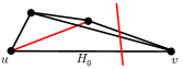
(a)

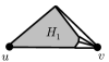
(b)

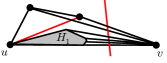
(c)

Figure 8: Illustration to the proof of Lemma 4. (a) A biplanar drawing of a part of $H_{0}$ with base $\{u,v\}$, (b) a specialized drawing of $H_{1}$ with base $\{u,v\}$, and (c) the composition of $H_{0}$ and $H_{1}$, so that $H_{1}$ is drawn in the first inner face of $H_{0}$.

We now proceed by induction on the number of inner components at every separation pair, and by recursion on inner components at separation pairs.

Theorem 3.1

Every 1-planar graph has a tri-fan-crossing straight-line biplanar drawing. The drawing uses numbers with $O(n\log n)$ many digits and can be computed in linear time.

Proof

Assume that $G$ is planar-maximal 1-planar. Otherwise, use the planarization and compute a planar-maximal augmentation from a 1-planar drawing. Decompose $G$ into its 3-connected components and store it in a decomposition tree, which may be an SPQR-tree [49]. Let $H_{0}$ be the outer component which remains from $G$ if all inner components at separation pairs are removed. Then $H_{0}$ is triconnected. Compute a straight-line specialized biplanar grid drawing of $H_{0}$ according to Lemmas 1, 2 or 3.

Let $H_{1},\ldots,H_{k}$ be inner components at a separation pair $\langle u,v\rangle$ of $H_{0}$. Then $(u,v)$ is an uncrossed edge of the 1-planar drawing of $H_{0}$. By induction, every $H_{i}$ admits a specialized straight-line biplanar drawing with a horizontal line for $(u,v)$. If $H_{i}$ has a pair of crossed edge in its outer face, then choose the last vertex so that the edges incident to $v$ are black. By induction, there are specialized biplanar drawings $\Gamma(H_{0},\ldots,H_{i})$ and $\Gamma(H_{i+1})$, which can be composed to a specialized biplanar drawing of $H_{0},\ldots,H_{i+1}$ by Lemma 4. By induction there is a tri-fan-crossing straight-line biplanar drawing for the inner components at a separation pair of $H_{0}$.

Note that two separation pairs are independent in the sense that there are distinct first inner faces, so that the biplanar drawings of components at two separation pairs do not interfere. By induction and Lemma 4, there is a tri-fan-crossing straight-line biplanar drawing $\Gamma(G)$.

A 1-planar graph with a single W-configuration can be drawn on a grid of size $O(n^{7})$ by Lemma 3. For every single inner component there is a scaling by $O(n^{5})$ by Lemma 4. Otherwise, a scaling by $O(n^{2})$ suffices. By induction and recursion this leads to a scaling of $O(n^{n})$, since at least six vertices are necessary for a W-configuration. Hence, the coordinates of the drawing have $O(n\log n)$ many digits.

It takes linear time to compute $\Gamma(G)$ from a 1-planar drawing of $G$, since every step can be done in linear time, such as the planar-maximal augmentation, the SPQR-decomposition, the biplanar drawing of single inner components, and the scaling by an affine transformation.

Corollary 1

Every 1-planar graph has geometric thickness at most two.

By a planarity test, we obtain:

Corollary 2

The thickness and the geometric thickness of a 1-planar graph can be computed in linear time.

4 Conclusion

We have shown that every 1-planar graph admits a straight-line biplanar drawing, that is it has geometric thickness two. The following problems remain.

(1) Does every 1-planar graph admit a straight-line biplanar drawing on a grid of polynomial size?

(2) Does every 1-planar graph admit a rectangle visibility representation? Rectangle visibility [37] specializes T-shape visibility [50].

(3) What is the geometric (general, book) thickness of other beyond planar graphs, for example $k$-planar, fan-crossing, fan-crossing free and quasi-planar graphs [51]?

References

- [1] E. Steinitz, H. Rademacher, Vorlesungen über die Theorie der Polyeder, Julius Springer, Berlin, 1934. doi:10.1007/978-3-642-65609-5.
- [2] K. Wagner, Bemerkungen zum Vierfarbenproblem, Jahresbericht Deutsche Math.-Vereinigung 46 (1936) 26–32.
- [3] I. Fáry, On straight line representation of planar graphs, Acta Sci. Math. Szeged 11 (1948) 229–233.
- [4] S. Stein, Convex maps, Proc. Amer. Math. Soc. 2 (1951) 464–466. doi:10.2307/2031777.
- [5] N. Chiba, K. Onoguchi, T. Nishizeki, Drawing plane graphs nicely, Acta Informatica 22 (2) (1985) 187–201. doi:10.1007/BF00264230.
- [6] N. Chiba, T. Yamanouchi, T. Nishizeki, Linear time algorithms for convex drawings of planar graphs, in: Progress in Graph Theory, Acadedmic Press, 1984, pp. 153–173.
- [7] W. T. Tutte, Convex representations of graphs, Proc. London Math. Soc 10 (1960) 302–320.
- [8] W. T. Tutte, How to draw a graph, Proc. London Math. Soc. 13 (1963) 743–768.
- [9] H. de Fraysseix, J. Pach, R. Pollack, How to draw a planar graph on a grid, Combinatorica 10 (1990) 41–51. doi:10.1007/BF02122694.
- [10] W. Schnyder, Embedding planar graphs on the grid, in: ACM-SIAM Symposium on Discrete Algorithms, SODA 1990, SIAM, 1990, pp. 138–147. doi:citation.cfm?id=320176.320191.
- [11] N. Bonichon, S. Felsner, M. Mosbah, Convex drawings of 3-connected plane graphs, Algorithmica 47 (4) (2007) 399–420. doi:10.1007/s00453-006-0177-6.
- [12] M. Chrobak, G. Kant, Convex grid drawings of 3-connected planar graphs, Internat. J. Comput. Geom. Appl. 7 (3) (1997) 211–223. doi:10.1142/S0218195997000144.
- [13] G. Kant, Drawing planar graphs using the canonical ordering, Algorithmica 16 (1996) 4–32. doi:10.1007/BF02086606.
- [14] C. Thomassen, Rectilinear drawings of graphs, J. Graph Theor. 12 (3) (1988) 335–341. doi:10.1002/jgt.3190120306.
- [15] S.-H. Hong, P. Eades, G. Liotta, S.-H. Poon, Fáry’s theorem for 1-planar graphs, in: J. Gudmundsson, J. Mestre, T. Viglas (Eds.), COCOON 2012, Vol. 7434 of LNCS, Springer, 2012, pp. 335–346. doi:10.1007/978-3-642-32241-9_29.
- [16] W. Didimo, Density of straight-line 1-planar graph drawings, Inform. Process. Lett. 113 (7) (2013) 236–240. doi:10.1016/j.ipl.2013.01.013.
- [17] R. Bodendiek, H. Schumacher, K. Wagner, Über 1-optimale Graphen, Mathematische Nachrichten 117 (1984) 323–339. doi:10.1002/mana.3211170125.
- [18] F. J. Brandenburg, On fan-crossing graphs, Theor. Comput. Sci. 841 (2020) 39–49. doi:10.1016/j.tcs.2020.07.002.
- [19] F. J. Brandenburg, Fan-crossing free graphs and their relationship to other classes of beyond-planar graphs, Theor. Comput. Sci. 867 (2021) 85–100. doi:10.1016/j.tcs.2021.03.031.
- [20] O. Cheong, S. Har-Peled, H. Kim, H. Kim, On the number of edges of fan-crossing free graphs, Algorithmica 73 (4) (2015) 673–695. doi:10.1007/s00453-014-9935-z.
-
[21]
M. A. Bekos, M. Kaufmann, C. N. Raftopoulou,
On optimal 2- and 3-planar
graphs, in: B. Aronov, M. J. Katz (Eds.), SoCG 2017, Vol. 77 of LIPIcs,
Schloss Dagstuhl - Leibniz-Zentrum für Informatik, 2017, pp.
16:1–16:16.
URL https://doi.org/10.4230/LIPIcs.SoCG.2017.16 - [22] F. J. Brandenburg, A first order logic definition of beyond-planar graphs, J. Graph Algorithms Appl. 22 (1) (2018) 51–66. doi:10.7155/jgaa.00455.
- [23] F. J. Brandenburg, On fan-crossing and fan-crossing free graphs, Inf. Process. Lett. 138 (2018) 67–71. doi:10.1016/j.ipl.2018.06.006.
- [24] M. Kaufmann, T. Ueckerdt, The density of fan-planar graphs, Tech. Rep. arXiv:1403.6184 [cs.DM], Computing Research Repository (CoRR) (March 2014).
- [25] E. Ackerman, J. Fox, J. Pach, A. Suk, On grids in topological graphs, Comput. Geom. 47 (7) (2014) 710–723. doi:10.1016/j.comgeo.2014.02.003.
- [26] J. Pach, R. Pinchasi, M. Sharir, G. Tóth, Topological graphs with no large grids, Graphs and Combinatorics 21 (3) (2005) 355–364. doi:10.1007/s00373-005-0616-1.
- [27] W. T. Tutte, The thickness of a graph, Indag. Math. 25 (1963) 567–577.
- [28] P. Mutzel, T. Odenthal, M. Scharbrodt, The thickness of graphs: A survey, Graphs and Combinatorics 14 (1) (1998) 59–73. doi:10.1007/PL00007219.
- [29] A. Aggarwal, M. M. Klawe, P. W. Shor, Multilayer grid embeddings for VLSI, Algorithmica 6 (1) (1991) 129–151. doi:10.1007/BF01759038.
- [30] C. S. J. A. Nash-Williams, Edge-disjoint spanning trees of finite graphs, Journal of the London Mathematical Society 36 (1) (1961) 445–450. doi:10.1112/jlms/s1-36.1.445.
- [31] H. N. Gabow, H. H. Westermann, Forests, frames, and games: Algorithms for matroid sums and applications, Algorithmica 7 (1992) 465–497. doi:10.1007/BF01758774.
- [32] P. Kainen, Thickness and coarseness of graphs, Abh. Math. Sem. Univ. Hamburg 39 (1973) 88–95.
- [33] D. Eppstein, Separating thickness from geometric thickness, in: S. G. Kobourov, M. T. Goodrich (Eds.), GD 2002, Vol. 2528 of Lecture Notes in Computer Science, Springer, 2002, pp. 150–161. doi:10.1007/3-540-36151-0_15.
- [34] V. Alekseev, V. Gonc̆akov, The thickness of arbitrary complete graphs, Math. Sbornik 30 (2) (1976) 187–202.
- [35] M. B. Dillencourt, D. Eppstein, D. D. Hirschberg, Geometric thickness of complete graphs, J. Graph Algorithms Appl. 4 (3) (2000) 5–15. doi:10.7155/jgaa.00023.
- [36] F. Harary, Research problem, Bull. Amer. Math. Soc. 67 (542).
- [37] J. P. Hutchinson, T. Shermer, A. Vince, On representations of some thickness-two graphs, Computational Geometry 13 (1999) 161–171. doi:10.1016/S0925-7721(99)00018-8.
- [38] M. Yannakakis, Embedding planar graphs in four pages, J. Comput. System. Sci 31 (1) (1989) 36–67. doi:10.1016/0022-0000(89)90032-9.
-
[39]
M. A. Bekos, M. Kaufmann, F. Klute, S. Pupyrev, C. N. Raftopoulou, T. Ueckerdt,
Four
pages are indeed necessary for planar graphs, J. Comput. Geom. 11 (1) (2020)
332–353.
URL https://journals.carleton.ca/jocg/index.php/jocg/article/view/504 - [40] M. Yannakakis, Planar graphs that need four pages, J. Comb. Theory, Ser. B 145 (2020) 241–263. doi:10.1016/j.jctb.2020.05.008.
- [41] M. A. Bekos, T. Bruckdorfer, M. Kaufmann, C. N. Raftopoulou, The book thickness of 1-planar graphs is constant, Algorithmica 79 (2) (2017) 444–465. doi:10.1007/s00453-016-0203-2.
- [42] M. J. Alam, F. J. Brandenburg, S. G. Kobourov, Straight-line drawings of 3-connected 1-planar graphs, in: S. Wismath, A. Wolff (Eds.), Proc. 21st GD 2013, Vol. 8242 of LNCS, Springer, 2013, pp. 83–94. doi:10.1007/978-3-319-03841-4_8.
- [43] R. Bodendiek, H. Schumacher, K. Wagner, Bemerkungen zu einem Sechsfarbenproblem von G. Ringel, Abh. aus dem Math. Seminar der Univ. Hamburg 53 (1983) 41–52. doi:10.1002/mana.3211170125.
- [44] J. Pach, G. Tóth, Graphs drawn with a few crossings per edge, Combinatorica 17 (1997) 427–439. doi:10.1007/BF01215922.
- [45] I. Bárány, G. Rote, Strictly convex drawings of planar graphs, Documenta Mathematica 11 (2006) 369–391.
- [46] E. Ackerman, A note on 1-planar graphs, Discrete Applied Mathematics 175 (2014) 104–108. doi:10.1016/j.dam.2014.05.025.
- [47] M. Chrobak, G. Kant, S. Nakano, Minimum-width grid drawings of plane graphs, Comput. Geomet. 11 (1998) 29–54. doi:10.1016/S0925-7721(98)00016-9.
- [48] M. Chrobak, T. Payne, A linear-time algorithm for drawing a planar graph on a grid, Inform. Process. Lett. 54 (1995) 241–246. doi:10.1016/0020-0190(95)00020-D.
- [49] G. Di Battista, P. Eades, R. Tamassia, I. G. Tollis, Graph Drawing: Algorithms for the Visualization of Graphs, Prentice Hall, 1999.
-
[50]
F. J. Brandenburg, T-shape
visibility representations of 1-planar graphs, Comput. Geom. 69 (2018)
16–30.
doi:10.1016/j.comgeo.2017.10.007.
URL https://doi.org/10.1016/j.comgeo.2017.10.007 - [51] W. Didimo, G. Liotta, F. Montecchiani, A survey on graph drawing beyond planarity, ACM Comput. Surv. 52 (1) (2019) 4:1–4:37. doi:10.1145/3301281.