ALLWAS: Active Learning on Language models in WASserstein space

Abstract

Active learning has emerged as a standard paradigm in areas with scarcity of labeled training data, such as in the medical domain. Language models have emerged as the prevalent choice of several natural language tasks due to the performance boost offered by these models. However, in several domains, such as medicine, the scarcity of labeled training data is a common issue. Also, these models may not work well in cases where class imbalance is prevalent. Active learning may prove helpful in these cases to boost the performance with a limited label budget. To this end, we propose a novel method using sampling techniques based on submodular optimization and optimal transport for active learning in language models, dubbed ALLWAS. We construct a sampling strategy based on submodular optimization of the designed objective in the gradient domain. Furthermore, to enable learning from few samples, we propose a novel strategy for sampling from the Wasserstein barycenters. Our empirical evaluations on standard benchmark datasets for text classification show that our methods perform significantly better ($>20\%$ relative increase in some cases) than existing approaches for active learning on language models.

1 Introduction

Active learning is a technique for improving model performance over a fixed annotation budget Cohn et al. (1996). Generally, the data is obtained for labeling iteratively after alternating training phases until the desired performance is achieved. This contrasts with passive learning, where one assumes access to labels for the entire pool of data. There are three scenarios for active learning Settles (2009): (1) pool-based, where a set of unlabeled data points are available (2) stream-based, in which the data points are received in an online fashion, and (3) membership query synthesis, where the data points are generated for labeling. In this work, our focus will be on the pool-based setting for active learning.

Active learning has benefited a wide gamut of applications such as text classification Tong and Koller (2002); Hoi et al. (2006), named entity recognition Tomanek and Hahn (2009); Shen et al. (2004), and machine translation Haffari and Sarkar (2009), to name a few. Transformer-based language models Devlin et al. (2019) have shown improved performance on NLP tasks. These models with a large number of parameters require comparable amounts of data to produce good results Margatina et al. (2021) and thus pose a challenge in the active learning setting. There has been a recent surge in the study of language models in the active learning setup Ein-Dor et al. (2020); Margatina et al. (2021). However, many of these approaches are based on uncertainty sampling, which may not work well for uncalibrated deep models Guo et al. (2017). Other approaches look at the embedding space Sener and Savarese (2018) or the gradient space Huang et al. (2016). However, these methods generally assume a Euclidean metric between the data points in the respective spaces, which fails to judiciously capture the complex interactions. In this paper, we hypothesize that finding a core set of points using the Wasserstein metric would result in better performance than simply selecting a set of points that minimizes or maximizes a measure.

Such large language models require considerable amounts of representative data, which makes it infeasible for fine-tuning in the active learning scenario that work with a limited annotation budget. This drawback is effectively alleviated by data augmentation in the image domain Ratner et al. (2017). However, data augmentation is not a straightforward exercise for textual data. There have been numerous attempts to augment data by generating samples to label in the token space Liu et al. (2020); Quteineh et al. (2020) and the feature space Kumar et al. (2019b); Feng et al. (2021). Generating tokens could render the labels erroneous because of the nature of the hard assignment. To this end, we propose an over-sampling strategy based on Wasserstein barycenters Cuturi and Doucet (2014) in the embedding space. Our rationale here is that augmenting data by such a sampling technique benefits active learning because it operates well in both the low data regime as well as the class imbalance scenarios.

To the best of our knowledge we are the first to propose such an augmentation method for active learning with language models. Our key contributions are:

1. We propose a novel sampling strategy based on the Wasserstein distance in the gradient space. We prove its submodularity and propose a $1-\frac{1}{e}$ optimal greedy algorithm.

2. We design an over-sampling technique based on the Wasserstein barycenter of the embeddings of the data points for better performance in the cases with few labeled samples.

3. We demonstrate the effectiveness of our method by running extensive experiments on real world scenarios of few labeled samples and class imbalance. We also conduct experiments on the multi-class settings which have not been considered in previous works.

2 Related Work

Prior works on active learning have focused on uncertainty based sampling such as entropy Lewis and Gale (1994), least model confidence Settles et al. (2008) and diversity based methods Settles et al. (2008); Xu et al. (2007); Wei et al. (2015). Settles et al. (2008); Hsu and Lin (2015) have tried to use a combination of the diversity and uncertainty based approaches. Active learning has been effectively used in previous works for CNN based models Sener and Savarese (2018); Gal and Ghahramani (2016); Gissin and Shalev-Shwartz (2019). Coresets have been used for importance sampling Cohen et al. (2017), $k$-means and medians clustering Har-Peled and Mazumdar (2004) and for Gaussian mixture models (GMMs) Lucic et al. (2018). Work in Mirzasoleiman et al. (2020) used coresets in the gradient domain for subsampling data points for accelerated training. Wei et al. (2015) combines the uncertainty sampling methods with a submodular optimization method for subset selection. Ramalingam et al. (2021) uses a combination of submodular functions for balancing constraints of class labels and decision boundaries using matroids. A study of the theoretical performance of batch mode active learning with submodularity is given in Chen and Krause (2013). Submodular functions have also been used in NLP for text summarization Lin and Bilmes (2011), machine translation Kirchhoff and Bilmes and goal oriented chatbots Dimovski et al. (2018). In contrast to previous works we propose a novel submodular function for query sampling that operates in the gradient space. We argue that this would help select samples that are most representative of the gradients.

Data Augmentation techniques using Wasserstein barycenters and optimal transport have been adopted in the literature Zhu et al. (2020); Bespalov et al. (2021); Nadeem et al. (2020); Yan et al. (2019) for the image domain. In contrast, NLP researchers have primarily focused on generating data in the token space Liu et al. (2020); Quteineh et al. (2020) for data augmentation Wang and Yang (2015); Kobayashi (2018), paraphrase generation Kumar et al. (2019a) etc. There exist methods that use mixups in the feature space Kumar et al. (2019b); Feng et al. (2021) for data augmentation. However, to the best of our knowledge this is the first work to explore data augmentation using Wasserstein barycenters for active learning using language models. We argue that our method is advantageous in the low sample and imbalanced class settings.

3 Problem Statement and Approach

3.1 Problem Formulation

Typical pool based active learning methods have the following components: a pool of unlabelled data $U_{pool}$, a model $M$ on which to train the data for the downstream task, and an annotation budget $b$, which is a limit on the amount of labeled data that can be obtained. The last component is an acquisition or query function $q(.)$ that would be used for querying over $U_{pool}$ to obtain the data to be labeled. This is an iterative process in which, at every iteration, the query function $q(.)$ acquires a query set of size $k(<b)$. Finally, the model $M$ is trained over the samples provided by the query function and is evaluated on a validation set $D_{val}$. The aim is to maximize the performance on $D_{val}$ with a minimum labeled sample set Siddhant and Lipton (2018). The process is repeated until the annotation budget $b$ is exceeded or the desired performance on the validation set is achieved.

3.2 Approach

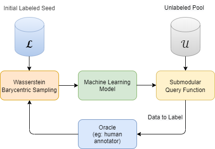
Figure 1: ALLWAS Process Flow. It uses Wasserstein Barycenters for data augmentation. The submodular query function is used for unlabeled data acquisition. These two steps aims to enhance performance of underlying ML model (BERT in our case).

Figure 1 outlines the flow of our proposed approach. First, the initial labeled seed of data is given to the barycentric sampling module for upsampling. Next, a model, in this case, a language model, is trained on this initial seed. The query function then uses the model to sample data points labeled by an oracle and a human annotator. The newly labeled data points are fed to the upsampling module, and the process repeats until the labeling budget is reached or the desired performance is achieved. The details of the individual components, along with some preliminaries, are explained in the following sections.

3.2.1 Optimal Transport and Wasserstein Barycenters

Let $\Omega$ be any space, $D$ be a distance metric in $\Omega$, and $P(\Omega)$ be the set of probability measures in that space. Let $x,y\in\Omega$ be the dirac masses with probability measures $\mu$ and $\nu$ respectively. The Optimal transport Monge (1781) problem is to minimize the cost in transporting $x$ to $y$ . The Wasserstein distance defines the optimal transport plan to move an amount of matter from one location to another.

Definition 3.1.

Let $p\in[1,\infty)$ and D: $\Omega\times\Omega$ $\xrightarrow{}[0,\infty)$ be the cost of transporting the measure $\mu$ to $\nu$, then the $p^{th}$ Wasserstein distance Villani between the measures is given by

$$W_{p}(\mu,\nu)=\inf_{\gamma\in\Pi(\mu,\nu)}\left(\int_{\Omega\times\Omega}D(x,y)^{p}\partial{\gamma}\right)^{\frac{1}{p}}$$ (1)

where $\Pi$ is the set of all the possible transport plans with the marginals $\mu$ and $\nu$.

Definition 3.2 (Wasserstein Barycenter, Agueh and Carlier (2011)).

A Wasserstein barycenter of $n$ measures $\{v_{1},v_{2},...,v_{n}\}$ in $\mathbb{P}\subset P(\Omega)$ is a measure that minimizes the weighted sum of the $p^{th}$ Wasserstein distance over $\mathbb{P}$ i.e. it is a minimiser of $f$ defined as below

$$f(\mu)=\sum_{i=1}^{N}\lambda_{i}W_{p}^{p}(\mu,\nu_{i})$$ (2)

Here we consider a convex combination of $W_{p}^{p}$ i.e. $\lambda_{i}\leq 1$ and $\sum_{i}\lambda_{i}=1$. If $D$ is the $L_{2}$ distance and $p=2$ that is when $P(\Omega,D)$ is the euclidean distance metric, minimizing $f$ results in the k means solution Kaufman and Rousseeuw (1987).

Sampling using Wasserstein Barycenters: The definition of the Wasserstein barycenter in 3.2 allows us to sample from a set of data points as illustrated in this section.

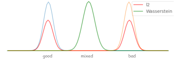
Figure 2: Example of a 1D Distribution (in orange and blue) showing the Wasserstein and $\ell_{2}$ barycenters

The intuition for using Wasserstein barycenters instead of euclidean barycenters is outlined in Figure 2. The figure shows a distribution of 1-dimensional word vectors, with the words ”good” and ”bad” at the extremes and the word ”mixed” in between them. We see from the distribution that the data contains the words ”good” and ”bad”. Sampling using the Wasserstein barycenter with equal weights gives us the word ”mixed.” In contrast, the $\ell_{2}$ barycenter would sample either of the words ”good” or ”bad” with equal probability. This implies that in a sentiment classification task, a pair of sentences ”The movie was good” and ”The movie was bad” would enable us to sample a neutral sentence ”The movie was mixed” using the Wasserstein barycenter. We argue that in contrast to sampling from the $\ell_{2}$ barycenter (see subsection 5.4) or no over-sampling (augmentation), sampling technique incorporating Wasserstein barycenters would result in superior performance for the few sample and imbalanced case.

Consider an machine learning (language) model such as Bert Devlin et al. (2019) with the output $d$ dimensional contextual embeddings as $e_{1},e_{2},\cdots e_{n}$ from a layer $l$ for the input tokens $w_{1},w_{2},\cdots w_{n}$ respectively. Now let us consider $s$ sentences each with number of tokens given by $n_{1},n_{2},\cdots n_{s}$ respectively. The contextual embeddings of a sentence $s_{i}$ would be represented as $E_{i}=[e_{1},e_{2},\cdots,e_{n_{i}}]$, where $E_{i}\in R^{d\times n_{i}}$. The Wasserstein barycenter of these samples would then be given by,

$$E_{c}=\underset{E_{c}\in R^{d\times n_{i}}}{argmin}\sum_{i=1}^{N}\lambda_{i}W_{p}^{p}(E_{c},E_{i})$$ (3)

Thus, we obtain the barycenter in the embedding space. We also modify the labels by taking a weighted average as follows:

$$L_{c}=\sum_{i=1}^{N}\lambda_{i}L_{i}$$ (4)

Where $L_{i}$ is the true class probabilities of the sentence $s_{i}$. Varying the values of the $\lambda$s could enable picking multiple data points, enabling over-sampling from the pool of labeled data.

3.2.2 Submodular Acquisition function

Let $V$ be the set of all points in the space $\Omega$ under consideration. Let $A$, $B$ be two subsets of V such that $A\subseteq B$. Let F be a set function (acting on a set $S$) $\Omega^{|S|}\xrightarrow[]{}R$, then F is said to be submodular if, on adding an element $e\in V\setminus B$ to $A$ and $B$, it satisfies the below condition

$$F\{A\cup e\}-F\{A\}\geq F\{B\cup e\}-F\{B\}$$

Previous works have used gradient spaces for subset selection in active learning Huang et al. (2016) and to speed up training Mirzasoleiman et al. (2020). Selecting a subset of points with gradients that are representative of the gradients of the entire set of points would intuitively result in steering the model parameters in the right direction of the optimum value. This motivates our approach of using the gradient space to perform the acquisition of the data points. One issue that remains is that unlike in Mirzasoleiman et al. (2020) we do not have the true labels beforehand. Huang et al. (2016) proposes to use the expected gradient length with the expectation over the predicted logits. However, the predicted probabilities do not always correlate with the model confidence Guo et al. (2017) and calibration of the model may be required. We differ in our approach where we use the Wasserstein distances between the points in the gradient space to find the most representative sample set. Specifically, we select the subset that minimizes the below function.

$$L\{S\}=\sum_{i\in V}\underset{j\in S}{min}(W_{p}^{p}(i,j))$$ (5)

where $W_{p}^{p}(i,j)$ is the $p^{th}$ Wasserstein distance between the $i^{th}$ and the $j^{th}$ sample in the gradient space. Minimizing L is equivalent to finding the k medoids Kaufman and Rousseeuw (1987) and in general, finding an exact solution is an NP-Hard problem. However, optimizing a submodular function enables us to obtain a $1-\frac{1}{e}$ optimal Nemhauser et al. solution in a greedy manner. We define a submodular function using $L$ as below:

$$F\{S\}=L\{s_{0}\}-L\{s_{0}\cup S\}$$ (6)

Here $s_{0}$ is an auxillary set element and $L\{s_{0}\}$ can be considered a constant. We prove the submodularity of equation 6 below.

Lemma 3.1.

The function $L\{S\}$ is monotone decreasing.

Proof.

From the definition of $L$ we have,

$$L=\sum_{i\in V}\underset{j\in S}{min}(W_{p}^{p}(i,j))$$

where $W_{p}^{p}(i,j)$ is the $p^{th}$ Wasserstein distance in the gradient space. On adding an element $e\in V\setminus S$ to $S$, we get the new set $S^{{}^{\prime}}=S\cup e$. The metric for the new set then becomes $L^{{}^{\prime}}=\sum_{i\in V}\underset{j\in S^{{}^{\prime}}}{min}(W_{p}^{p}(i,j))$. Now let’s assume that $L^{{}^{\prime}}>L$. This means that for some point $i\in V$, the newly added point $e$ was selected and the distance $W_{p}^{p}(i,e)$ is greater than the previous minimum $W_{p}^{p}(i,j)$, which is a contradiction. Thus, we have that $L^{{}^{\prime}}\leq L$. ∎

Corollary 3.1.

The function $F=L\{s_{0}\}-L\{S\cup s_{0}\}$ is monotone increasing.

Proof.

If we fix $L\{s_{0}\}$ to a constant and since $L\{S\}$ is monotone decreasing from lemma 3.1 , we have $F$ is monotone increasing. ∎

Proposition 3.1.

The rate of increase of $F$ at $A\in V$ is greater than or equal to that at $B(\in V)\supseteq A$.

To understand proposition 3.1 we note that adding $e\in V\setminus B$ to $A$ causes an increase in $F$ or maintains the value as it is monotone increasing from corollary 3.1 and since $A\subseteq B$ adding $e$ to $B$ will only cause the same or lesser increase in $F\{B\}$ by definition of $F$.

Theorem 3.1.

$F$ is a submodular function.

Proof.

Assume set of points in the gradient space, $B\in V$ and a set $A\subseteq B$. We assume a continuous space of the elements such that adding a fraction of it would cause a fractional change in the output. Note that an interpolation does not change the function definition for the discrete case where the direct mass is concentrated. Consider adding an element(s) $e\in V\setminus B$ to the sets $A$ and $B$. By the gradient theorem for path integral we get,

$$F(A\cup e)-F(A) =\int_{0}^{1}\frac{\partial F(A+\alpha(A\cup e-A))}{\partial\alpha}d\alpha$$

$$=\int_{0}^{1}\frac{\partial F(A+\alpha(A\cup e-A))}{\partial x}\frac{\partial x}{\partial\alpha}d\alpha$$

(using chain rule)

$$=(A\cup e-A)\int_{0}^{1}\frac{\partial F(A+\alpha(A\cup e-A))}{\partial x}d\alpha$$

$$\text{(as }\frac{\partial x}{\partial\alpha}=A\cup e-A=\text{constant }K\text{)}$$

$$=K\int_{0}^{1}\frac{\partial F(A+\alpha(A\cup e-A))}{\partial x}d\alpha$$

Similarly,

$$F(B\cup e)-F(B)=K\int_{0}^{1}\frac{\partial F(B+\alpha(B\cup e-B))}{\partial x}d\alpha$$

From proposition 3.1 we have $\frac{\partial F(A)}{\partial x}_{|x=A}\geq\frac{\partial F(B)}{\partial x}_{|x=B}$ for addition of the same element $e$ and this will be true in the entire interval $\alpha\in[0,1]$. Thus we get,

$$F(A\cup e)-F(A)\geq F(B\cup e)-F(B)$$

Thus we can conclude that $F$ is submodular. ∎

Since we have a submodular function in $F$, we could use a greedy algorithm to find a set that is $(1-\frac{1}{e})$ of the optimal set $S$ that maximizes $F$ (minimizes $L$). It further runs in polynomial time. The greedy algorithm begins with an empty set $S=\phi$ and at each iteration keeps adding an element $e\in V\setminus S$ that maximizes $F(e|S_{i-1})=F(e\cup S_{i-1})-F(S_{i-1})$ i.e. $S_{i}=S_{i-1}\cup\ \underset{e\in V}{argmax}F(e|S_{i-1})$. The iterations continue till a specified labeling budget is attained. In practice, computing the gradients with respect to the entire set of weights could be computationally expensive in language models that could have millions of parameters. Fortunately for deep networks most of the variation in gradients with respect to the loss is captured by the last layer Katharopoulos and Fleuret (2019). Also, Mirzasoleiman et al. (2020) efficiently upper bounds the norm of the difference between the gradients by the norm of the gradients of the loss with respect to the inputs to the last layer. Thus for computational efficiency we restrict to finding the gradients with respect to the weights of the last layer. The outline is sketched in Algorithm 1.

Input: Unlabeled pool $\mathcal{U}$, Total Budget $B$, Samples to label per iteration $k$, Model $M$, Initial labeled set $\mathcal{L}$;
while $|\mathcal{L}|\leq|B|$ do

1. Train model M on $\mathcal{L}$

2. $V\xleftarrow[]{}\phi$
   for $x\in\mathcal{U}$ do

           $e\xleftarrow[]{}\frac{\partial\mathcal{M}(x)}{\partial x}$

           $V=V\cup e$

           end for

$S_{0}\xleftarrow[]{}\mathcal{L}$

for i = 1, 2, …, k do

                $e=\underset{e\in V}{argmax}\ F(e|S_{i-1})$ $S_{i}=S_{i-1}\cup e$

                end for

$L\xleftarrow[]{}S$

      end while

Algorithm 1 Greedy Algorithm to sample from the pool of unlabeled data points for Active learning

4 Experimental Setup

4.1 Datasets

We use 7 standard text classification datasets and their 10 variants as used by Ein-Dor et al. (2020). Specifically, the datasets used are Wiki Attack Wulczyn et al. (2017), ISEAR Shao et al. (2015), TREC Li and Roth (2002), CoLA Warstadt et al. (2019) , AG’s News Zhang et al. (2015), Subjectivity Pang and Lee (2004), and Polarity Pang and Lee (2005). The experimental setup considers three settings: (1) Balanced, in which the prior probability of a class occurrence is $\geq$ 15%. Here the initial seed for labeling is obtained by random sampling. (2) Imbalanced and (3) Imbalanced practical in which the prior probability of a class occurrence is $\leq$ 15%. The initial seed for labeling is obtained by assuming a high precision algorithm or a query. For more details on the datasets and experimental setups, we refer the readers to Ein-Dor et al. (2020) and the Appendix.

4.2 Comparative Methods

The acquisition methods are used to query and obtain samples from the unlabeled pool for labeling. In the implementation 25 samples are queried per iteration. We use the active learning acquisition strategies as in Ein-Dor et al. (2020) namely Random, Least Confidence (LC, Lewis and Gale (1994)), Monte Carlo Dropout (Dropout, Gal and Ghahramani (2016)), Perceptron Ensemble (PE, Ein-Dor et al. (2020)), Expected Gradient Length (EGL, Huang et al. (2016)) , Core-Set (Sener and Savarese (2018)), Discriminative Active Learning (DAL, Gissin and Shalev-Shwartz (2019)). For details refer to the Appendix.

4.3 Implementation Details

The $\text{BERT}_{\text{BASE}}$ model (110 M parameters) is used with a batch size of 50 and a maximum token length of 100 tokens. In each active learning iteration, the model is trained for five epochs from scratch. A learning rate of $5\times 10^{-5}$ has been used. The other parameters are the same as in the PyTorch implementation of BERT. We run each active learning method for five runs starting from the same initial seed (of 25 samples) for every model for a given run and average the result as in Ein-Dor et al. (2020).

5 Results and Discussion

We aim to answer the below Research Questions:

1. RQ1: Is ALLWAS beneficial in the low resource and imbalanced setting?

2. RQ2: Does the proposed Wasserstein barycentric over-sampling help in the few sample settings compared to the control of no over-sampling?

3. RQ3: Does the proposed gradient-domain submodular query function perform better than existing approaches in the same space?

4. RQ4: Is barycentric over-sampling in the wasserstein space significantly better than that in the $\ell_{2}$ space?

5.1 Active Learning Results on the Binary class settings

The results, for the imbalanced practical binary setting, are shown in the graphs in figures 10. The results for the other settings can be found in the Appendix. For brevity we show the results on the same set of the active learning methods as in Ein-Dor et al. (2020). From the Figures in 10, we observe that in most of the datasets our method outperforms all the other methods in all settings. For the balanced setting, we find that our method performs exceptionally well in the start with lesser data. Then as the training data increases with iterations, the performance of the other methods catches up. Thus we could say that our method converges faster in scenarios where the data is balanced. In the two imbalanced settings, we observe an apparent gain in performance. Thus, we conclude that combining submodular query function and barycentric sampling benefits performance in class imbalance cases of active learning (answering RQ1).

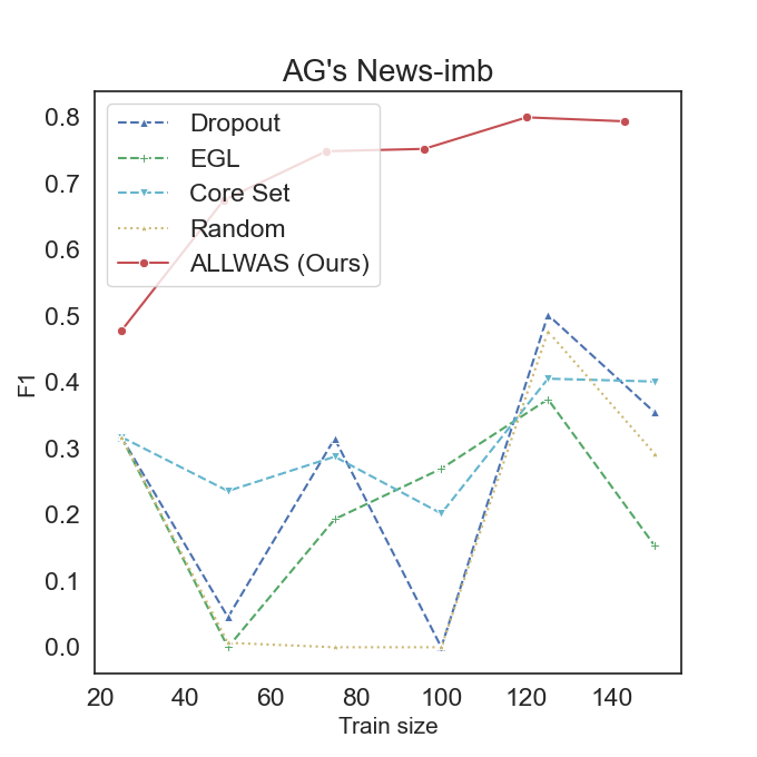
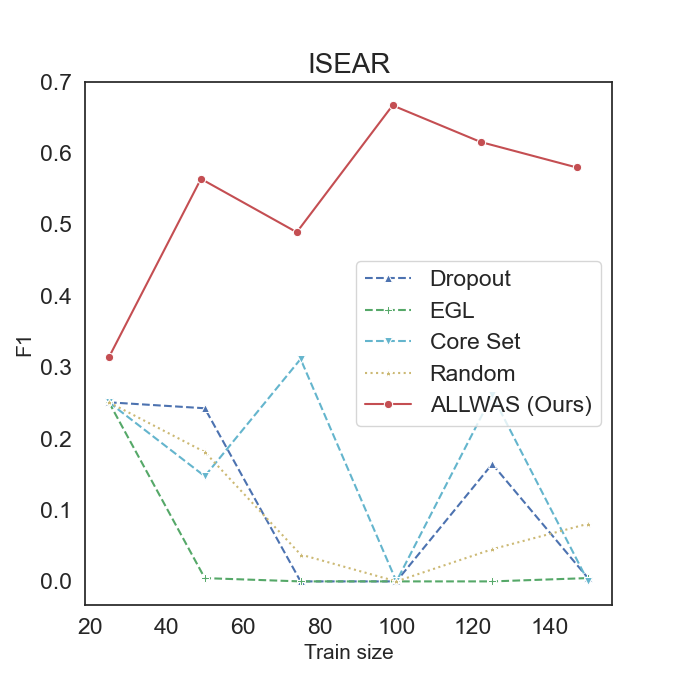
Figure 3: Results on the Imbalanced Practical setting. Our Model clearly outperforms the baselines.

5.2 Few Sample Results

In the few sample settings, we test the barycentric sampling on a few data points sampled incrementally. The augmentation factor is kept at 20 as a default. The results are plotted in Figure 4. We observe a stark improvement in the results, in some cases the relative increase being as high as 24%. This shows that in such cases of data scarcity, the task, in this case, classification, could benefit by sampling from the Wasserstein barycenter of the original samples as an augmentation technique independent of the sampling technique used in the query function (answering RQ2).

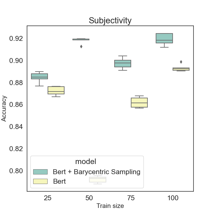
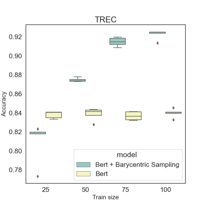
Figure 4: Few sample setting. Our setting (BERT+barycentric sampling) illustrates superior performance.

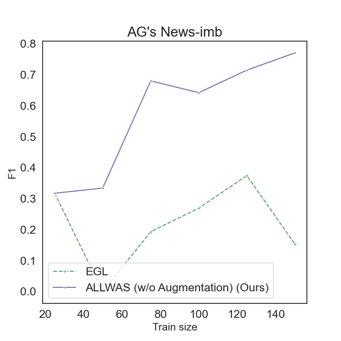
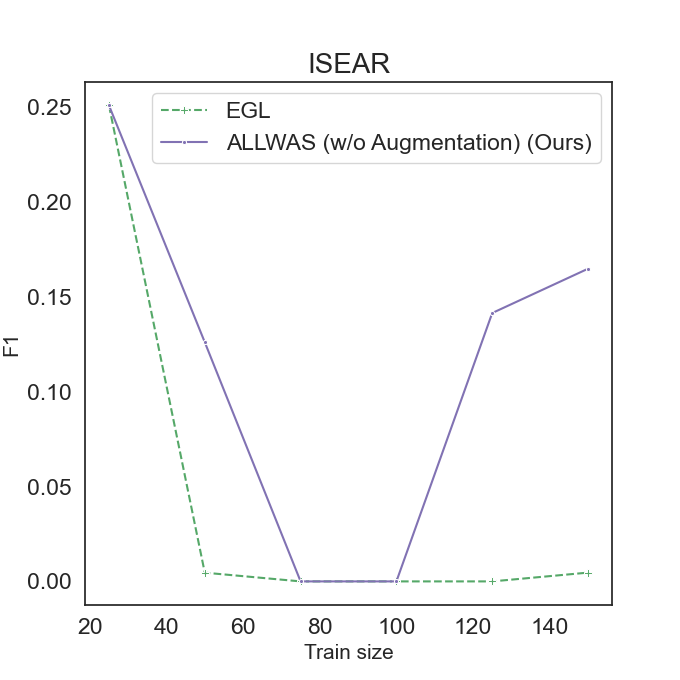
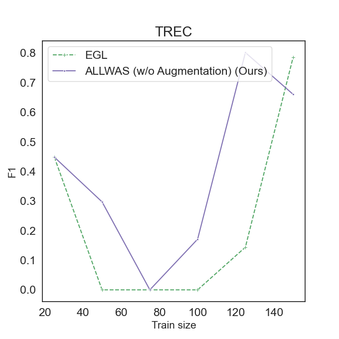
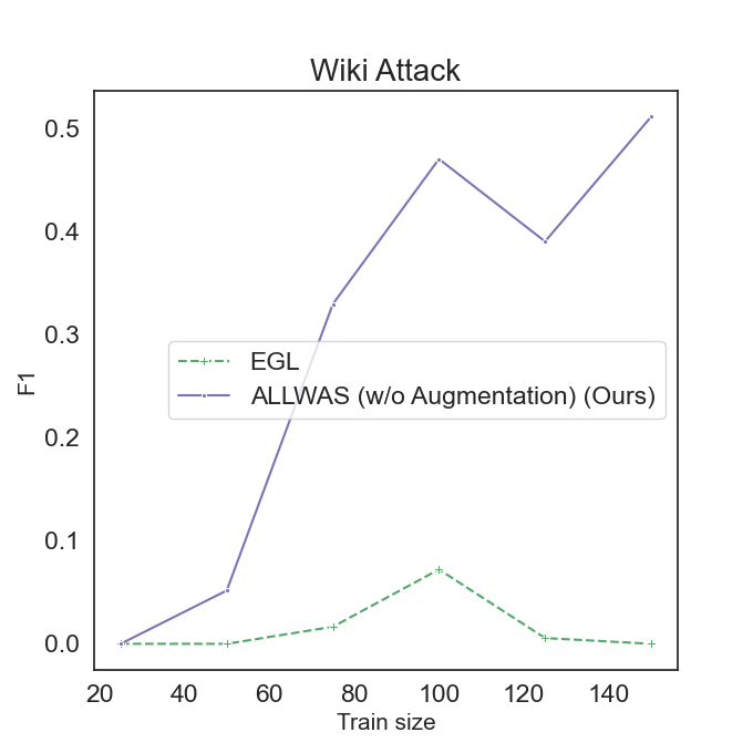
Figure 5: Comparison between selection based on maximum and coreset in the gradient domain

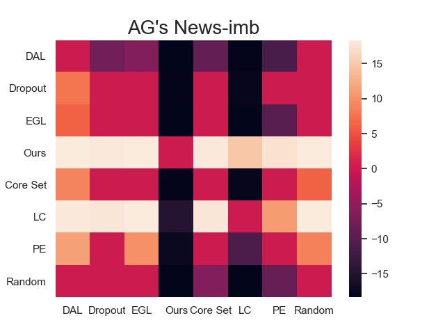
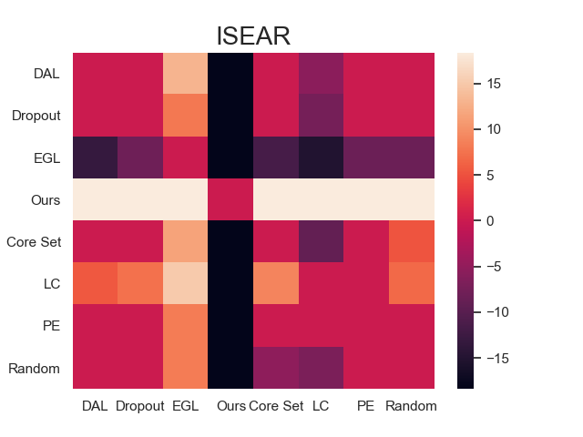
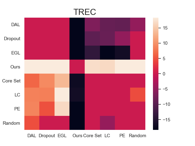
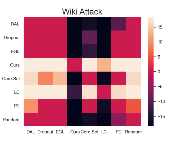
Figure 6: Statistical significance. Our model is statistically significant compared to baseline, illustrating the robustness of our proposed approach.

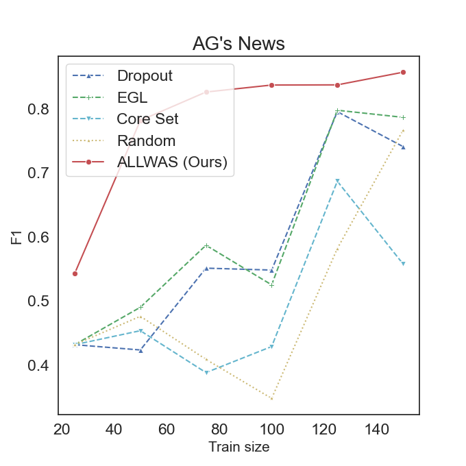
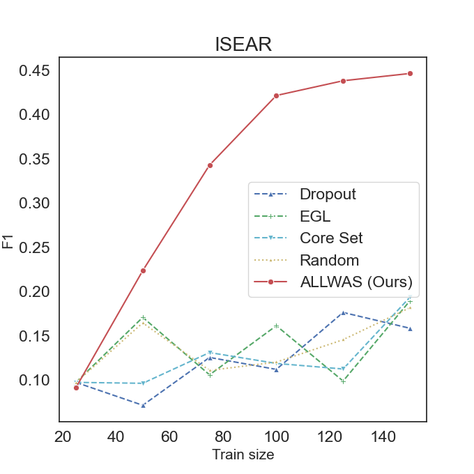
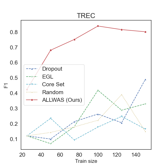
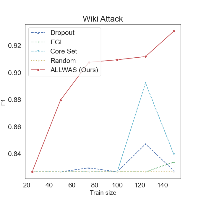
Figure 7: Results on the Multiclass setting. Our model performs significantly better than baselines.

5.3 Coreset vs Maximum Gradient

In this section, we study the performance of our query function (ALLWAS w/o Augmentation) that selects a coreset of the gradients against the expected gradient length method that picks samples with the largest expected gradient magnitudes (EGL, Huang et al. (2016)). The plots in figure 5 show that our query sampling technique outperforms the EGL method. Thus we conclude that selecting core-sets is the better approach against picking samples with extreme values in the gradient domain in assertion of RQ3.

5.4 Sampling from Wasserstein vs $\ell_{2}$ barycenter

In order to confirm the claim made in subsection 3.2.1, we perform a comparison between $\ell_{2}$ barycentric and Wasserstein barycentric over-sampling on the imbalanced practical setting. Sampling from $\ell_{2}$ is done by performing a kernel density estimation in the embedding space and then sampling from the resulting distribution. We report the Wilcoxon signed-rank test statistics in table 1 with Bonferroni correction to take into account the runs from all the datasets, settings, and iterations. Statistically significant (better) results are reported of the two sampling techniques against each other and a control of no over-sampling (augmentation). The results indicate that while both the over-sampling methods perform better than no sampling, reaffirming RQ2, sampling from the Wasserstein barycenter performs better than sampling from the $\ell_{2}$ barycenter confirming the claim in 3.2.1 and asserting RQ4.

Significance wrt	$\ell_{2}$	Wasserstein
No over-sampling	$<10^{-20}$	$<10^{-26}$
$\ell_{2}$	–	$<10^{-12}$
Wasserstein	–	–

Table 1: Comparison of over-sampling (for augmentation) from the $\ell_{2}$ vs Wasserstein barycenters, indicating p-values if the method of the column is significantly better than that of the row. – indicates statistically insignificant or worse performance

5.5 Statistical Significance

We study if the performance of our methods is statistically significant concerning the baselines for each dataset. We perform the Wilcoxon signed-rank test for significance with Bonferroni correction. We select the Wilcoxon test due to its nonparametric nature. The significant results in the form of heatmaps of the logarithms of the p-values are shown in figure 6. The insignificant results have their values at 0. From the heatmaps, our method outperforms the baselines in all datasets, indicating the increase is indeed statistically significant. The results echo the observation made by Ein-Dor et al. (2020) that no single sampling strategy is better than all others. However, in the low data regime that we operate in, many of the methods are not significantly better than the random sampling baseline.

5.6 Multi class Active Learning Results

Similar to the binary settings, we also study the performance of our method in the multi-class setting. We find that in the multi-class setting, too, our method works better than the baselines, as can be seen in figure 11. This shows that our method is not restricted to the binary classification setting but also to the more generic multi-class cases.

5.7 Effect of augmentation factor

We study the effect of the multiplicative factor while augmenting the samples using barycentric sampling technique. Here the number of samples of which to compute the barycenter is kept at two. The results are given in the appendix. It is observed that as the augmentation factor is increased, the performance increases initially when the data is low. However, as more data is acquired from the unlabeled pool, the gap reduces. This indicates that we may benefit more by keeping the augmentation factor high in the low data regime.

5.8 Effect of number of samples to find the barycenter

Similar to subsection 5.7, we study the effect of the number of data points used to find the barycenter. Keeping the augmentation factor fixed at 20, we vary the number of samples to find the barycenter. Results are in the Appendix. It is observed that as the data points to the sample increases, the performance marginally drops. This becomes intuitive if we think of computing the barycenter as averaging over the samples. If we average out many samples, we effectively get the representative sample which would be similar in most iterations.

6 Conclusion

This paper presents and studies novel approaches of data sampling using concepts from submodular optimization and optimal transport theory for active learning in language models. We find that augmenting data using the Wasserstein barycenter helps to learn in the few sample setting. Further, we conclude that using a submodular function based on the Wasserstein distance for sampling in the gradient domain helps in active learning. Future works could explore data subset distances using optimal transport to find the subset of data that would benefit the model. It also remains to be explored if using core-sets obtained in this manner would help speed up the training of language models without affecting its accuracy by a large margin. We point readers to the open questions in this domain as next viable steps.

Appendix A Appendix

A.1 Details of Dataset

We use seven standard text classification datasets and their ten variants as used by Ein-Dor et al. (2020). Specifically, the datasets used are Wiki Attack Wulczyn et al. (2017) which annotates wikipedia discussions for offensive content, ISEAR Shao et al. (2015) which reports for personal accounts of emotions, TREC Shao et al. (2015) which classifies question categories, CoLA Warstadt et al. (2019) which identifies the content for linguistic acceptability, AG’s News Zhang et al. (2015) which categorises news articles, Subjectivity Pang and Lee (2004) which classifies movie snippets into subjective and objective and Polarity Pang and Lee (2005) which provides sentiment categories of movie reviews. The datasets which contain labels with a prior of greater than 15% are taken into the balanced setting and those with less than a 15% prior are considered in the imbalanced setting as in Ein-Dor et al. (2020). The experimental setup considers 3 settings: (1) Balanced, in which the prior probability of a class occurrence is $\geq$ 15%. Here the initial seed for labeling is obtained by random sampling. (2) Imbalanced and (3) Imbalanced practical in which the prior probability of a class occurrence is $\leq$ 15%. In the case of the Imbalanced setting the initial seed is taken by randomly sampling from the class with the low prior. Here the assumption is that there exists a heuristic to obtain an unbiased sample set with high precision of the low prior class. As this may not always hold true the Imbalanced practical setting samples using a simple and empirical heuristic such as a query based search for the samples belonging to the low prior class. This gives a (biased) set of samples of the class which are then used for labeling . For the class with a high prior probability random samples are drawn from the dataset and are labeled as such for both the imbalanced settings.

No.	Dataset	Size	Class	Prior
1	Subjectivity-imb	5,556	subjective	10%
2	Polarity-imb	5,923	positive	10%
3	AG’s News-imb	17,538	world	10%
4	Wiki attack	21,000	general	12%
5	ISEAR	7,666	fear	14%
6	TREC	5,952	location	15%
7	AG’s News	21,000	world	25%
8	CoLA	9,594	unacceptable	30%
9	Subjectivity	10,000	subjective	50%
10	Polarity	10,662	positive	50%

Table 2: Dataset Statistics

A.2 Details of Comparative Methods

The acquisition methods are used to query and obtain samples from the unlabeled pool for labeling. In the implementation 25 samples are queried per iteration. We use the active learning acquisition strategies as in Ein-Dor et al. (2020) as below:

1. Random: The data for labeling are randomly sampled from the unlabeled pool.

2. Least Confidence (LC, Lewis and Gale (1994)): This method picks the top $k$ samples for which the model uncertainty is the highest.

3. Monte Carlo Dropout (Dropout, Gal and Ghahramani (2016)): This uses Monte Carlo dropout during inference for multiple runs and averages the probabilities followed by sampling the least certain instances.

4. Perceptron Ensemble (PE, Ein-Dor et al. (2020)): Here the output of an ensemble of models is used to pick the instances with highest uncertainty. To avoid the computational cost associated with training an ensemble of BERT models, this method uses the perceptron models trained on the CLS output of the finetuned BERT.

5. Expected Gradient Length (EGL, Huang et al. (2016)): The samples are selected based on the largest expected gradient norm as in Huang et al. (2016). The expectation is over the model predicted probabilities.

6. Core-Set (Sener and Savarese (2018)): This method picks samples that best cover the dataset in the embedding space (CLS) using the greedy method desribed in Sener and Savarese (2018).

7. Discriminative Active Learning (DAL, Gissin and Shalev-Shwartz (2019)): This technique selects samples that make the L most representative instances of the entire pool as per Gissin and Shalev-Shwartz (2019).

A.3 Additional Results

A.3.1 Active Learning Results on the Binary class settings

The results for the three binary settings are shown in the graphs in figures 8, 9 and 10. From the figures we observe that in most of the datasets our method outperforms all the other methods in all settings. We report the $f_{1}$ scores for all settings, since in the balanced case also there may be a slight class imbalance (upto $60\%$). For the balanced setting we find that our method performs exceptionally well in the start with lesser data and then as the training data increases with iterations the performance of the other methods catch up. Thus we could say that our method converges faster in scenarios where the data is balanced. There was one exception with the Cola dataset in which the metric drops as compared to others. Upon further investigating we find that the upsampling causes a drop in performance in this case. Thus, while sampling in this manner may cause an increase in performance in most of the cases it may require the practitioner to fine tune the factor by which to augment the data. In the other 2 settings, namely the imbalanced settings, we observe a clear gain in performance. Thus we conclude that the combination of our submodular query function and barycentric sampling benefits performance in active learning scenarios where there is prevalence of class imbalance.

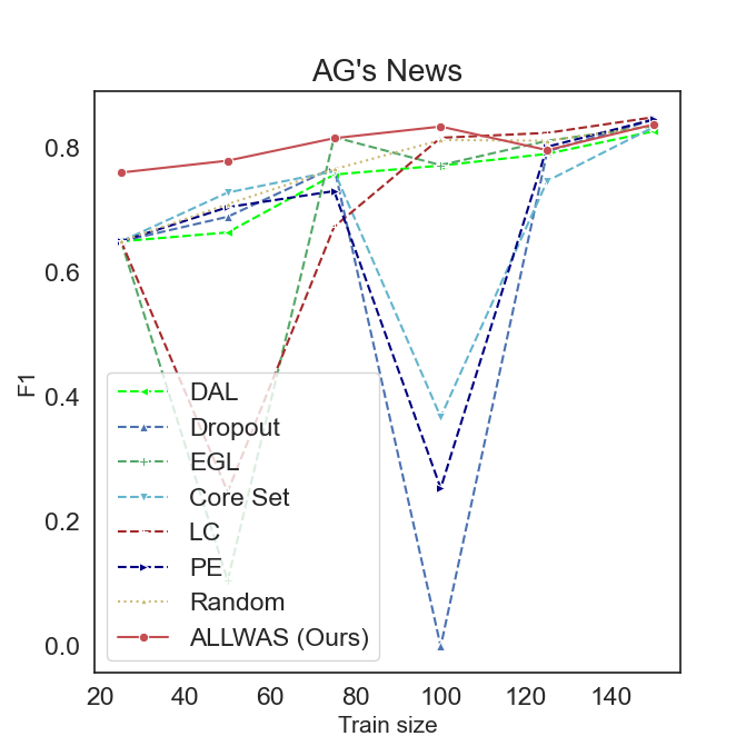
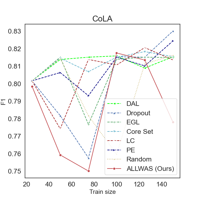
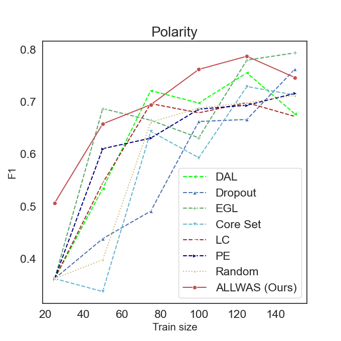
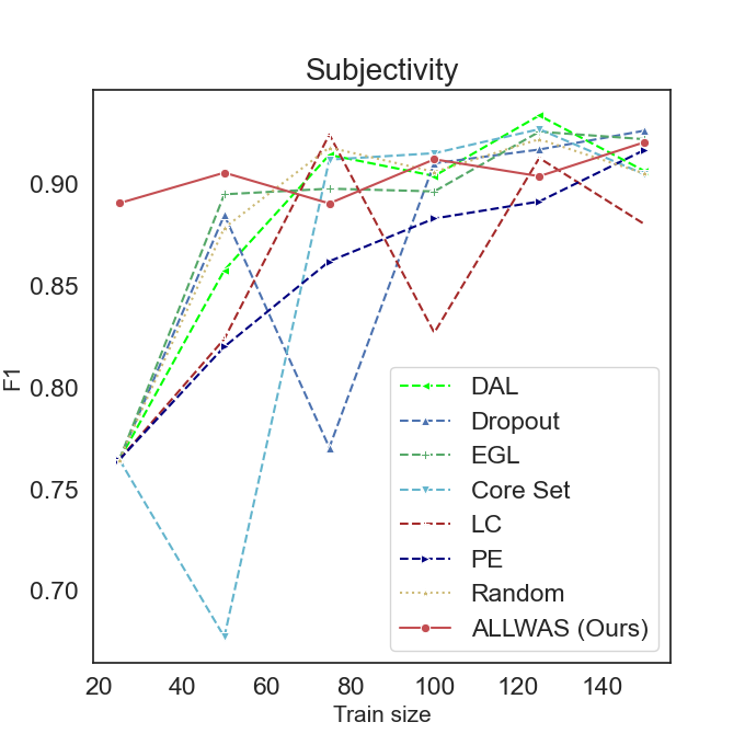
Figure 8: Results on the Balanced setting

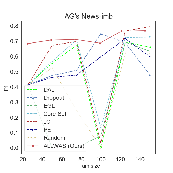
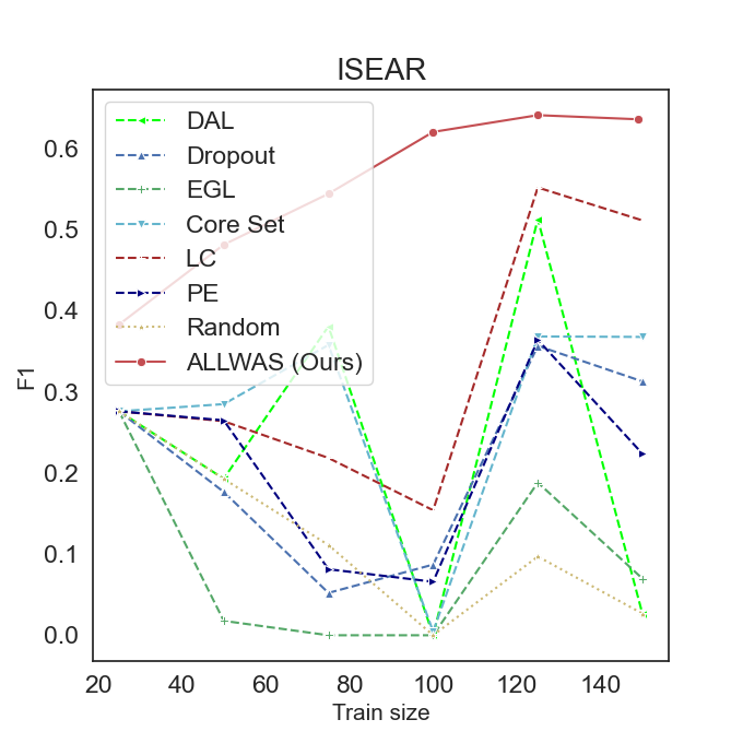
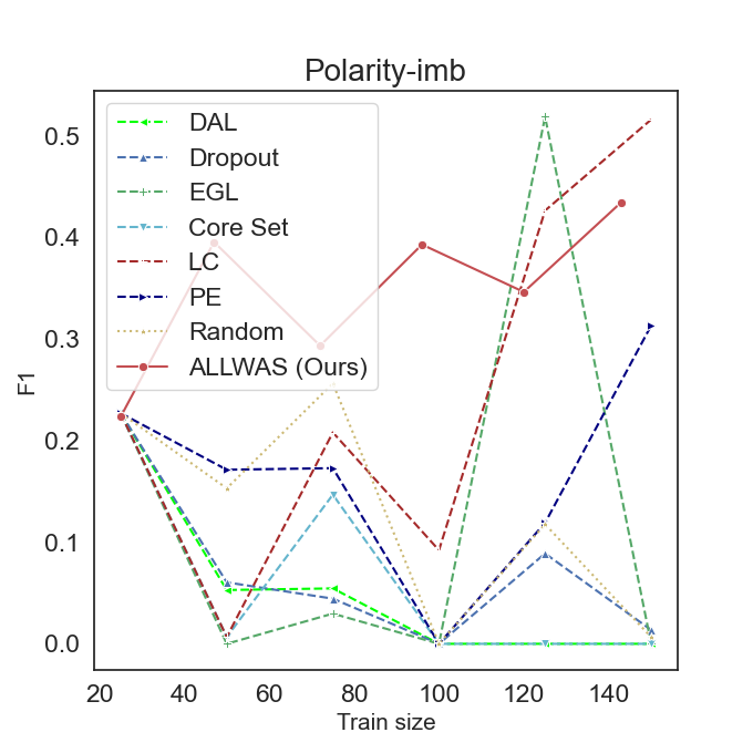
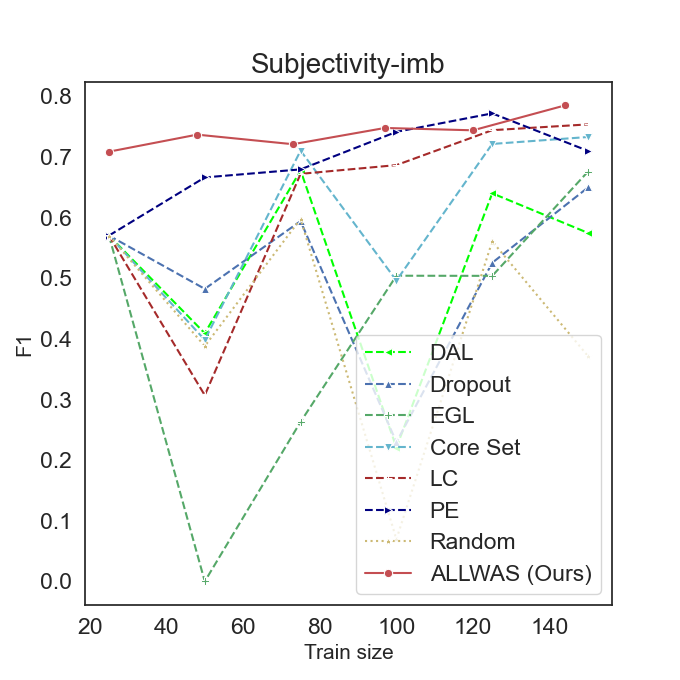
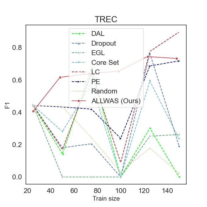
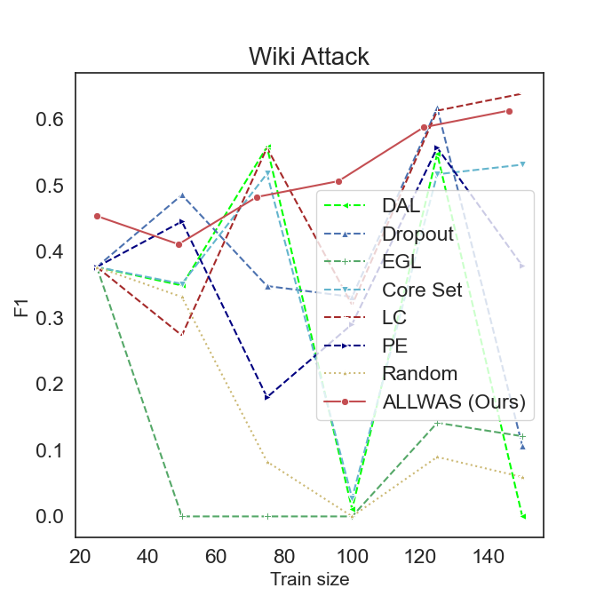
Figure 9: Results on the Imbalanced setting

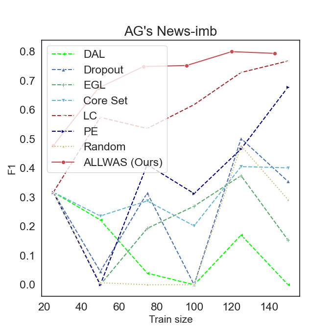
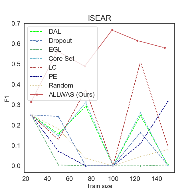
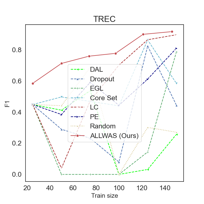
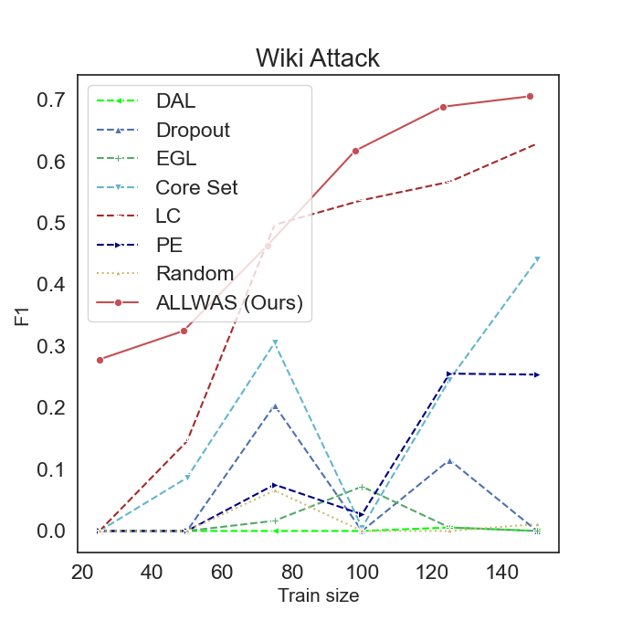
Figure 10: Results on the Imbalanced Practical setting

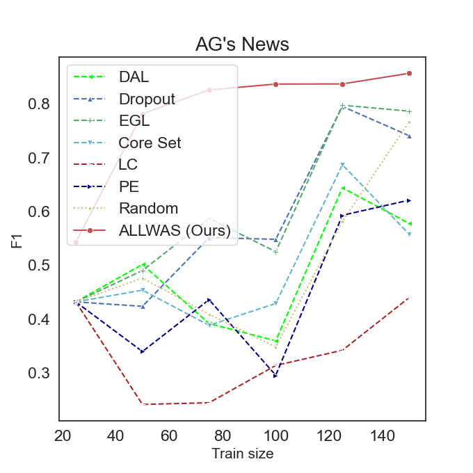
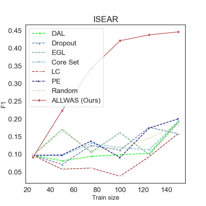
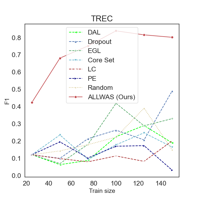
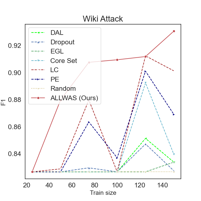
Figure 11: Results in the Multi-class setting

A.3.2 Multi class Active Learning Results

In addition to the results in the main paper, here we report the results on all methods for the multi-class setting in figure 11.

A.3.3 Effect of augmentation factor

We would like to study the effect of the multiplicative factor while augmenting the samples using barycentric sampling technique. Here the number of samples of which to compute the barycenter are kept at 2. The results are shown in figure 12. It can be seen that as the augmentation factor is increased the performance increases initially, when the data is low, but as more data is acquired from the unlabeled pool the gap reduces and also reverses. This indicates that we may benefit more by keeping the augmentation factor high in the low data regime.

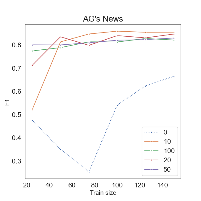
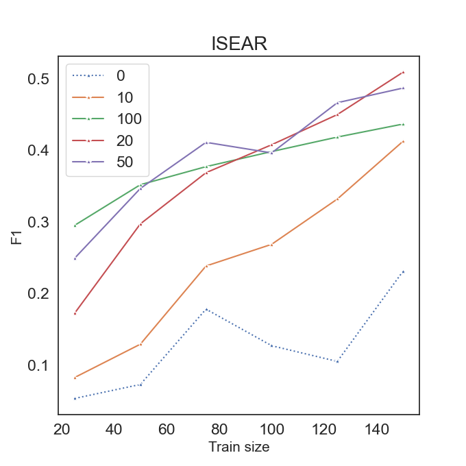
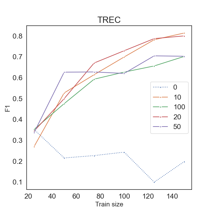
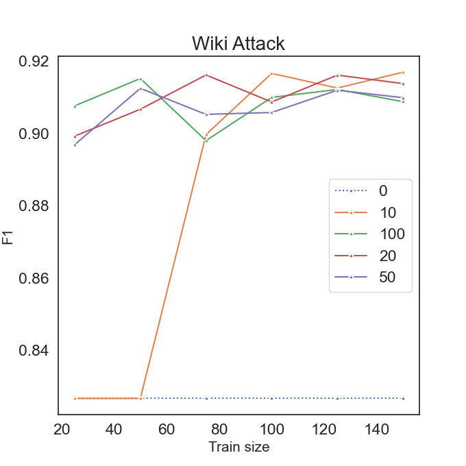
Figure 12: Ablation study on the augmentation factor

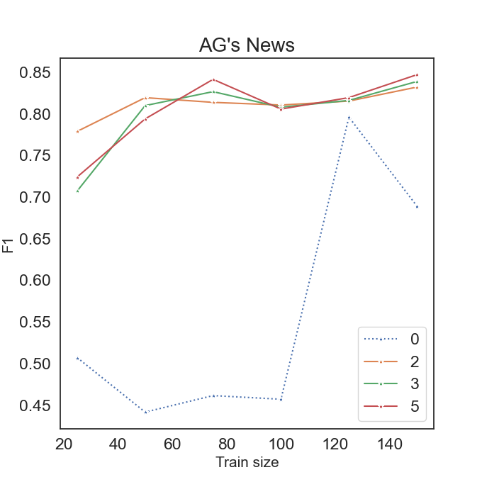
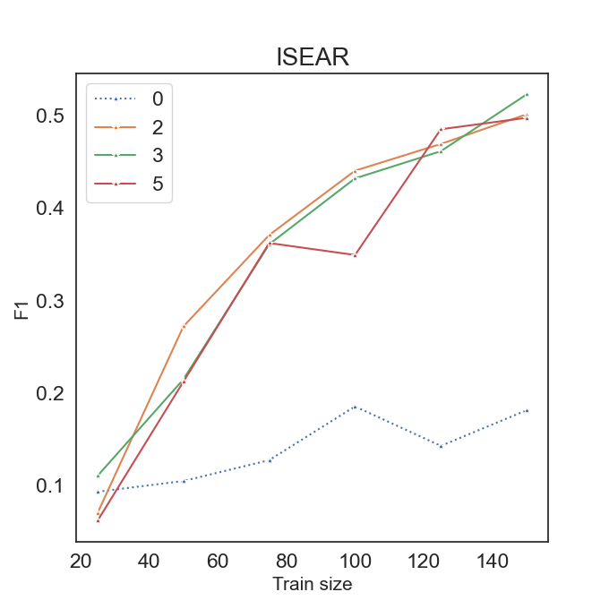
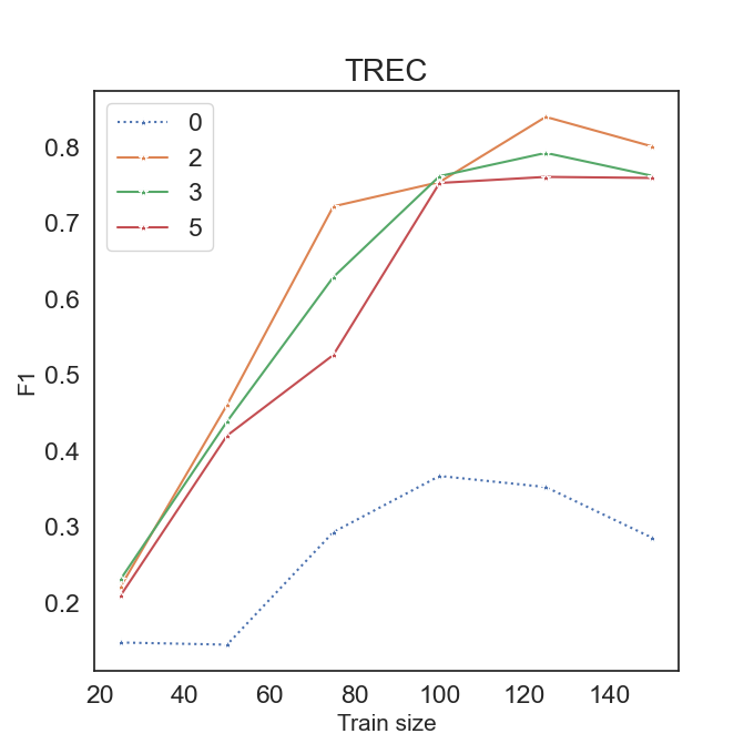
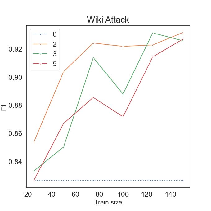
Figure 13: Ablation study on the number of samples to compute the barycenter

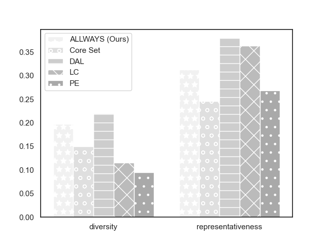
Figure 14: Diversity and Representativeness

A.3.4 Effect of number of samples to find the barycenter

Similar to section A.3.3, we would like to study the effect of the number of data points used to find the barycenter. Keeping the augmentation factor fixed at 20, we vary the number of samples to find the barycenter. As can be seen in figure 13, it can be understood that as the data points to sample from increases the performance marginally drops. This becomes intuitive if we think of computing the barycenter as averaging over the samples and if we average out many samples we effectively get the representative sample which would similar in most iterations especially in the labels space.

A.3.5 Diversity and Representativeness

We compute the diversity and representativeness of the selected samples as outlined in Ein-Dor et al. (2020). From figure 14 we see that our method gives comparable values of these metrics. DAL performs well on both the metrics as it was designed for maximising them. This shows there is some room for improvement in the proposed method with regards to the diversity and representativeness metrics. We leave this for future works.

References

- Agueh and Carlier (2011) Martial Agueh and Guillaume Carlier. 2011. Barycenters in the wasserstein space. SIAM Journal on Mathematical Analysis, 43(2):904–924.
- Bespalov et al. (2021) Iaroslav Bespalov, Nazar Buzun, Oleg Kachan, and Dmitry V. Dylov. 2021. Data augmentation with manifold barycenters.
- Chen and Krause (2013) Yuxin Chen and Andreas Krause. 2013. Near-optimal batch mode active learning and adaptive submodular optimization. In Proceedings of the 30th International Conference on Machine Learning, volume 28 of Proceedings of Machine Learning Research, pages 160–168, Atlanta, Georgia, USA. PMLR.
- Cohen et al. (2017) Michael B. Cohen, Cameron Musco, and Christopher Musco. 2017. Input sparsity time low-rank approximation via ridge leverage score sampling. In Proceedings of the Twenty-Eighth Annual ACM-SIAM Symposium on Discrete Algorithms, SODA ’17, page 1758–1777, USA. Society for Industrial and Applied Mathematics.
- Cohn et al. (1996) David A. Cohn, Zoubin Ghahramani, and Michael I. Jordan. 1996. Active learning with statistical models. J. Artif. Int. Res., 4(1):129–145.
- Cuturi and Doucet (2014) Marco Cuturi and Arnaud Doucet. 2014. Fast computation of wasserstein barycenters. In Proceedings of the 31st International Conference on Machine Learning, volume 32 of Proceedings of Machine Learning Research, pages 685–693, Bejing, China. PMLR.
- Devlin et al. (2019) Jacob Devlin, Ming-Wei Chang, Kenton Lee, and Kristina Toutanova. 2019. BERT: Pre-training of deep bidirectional transformers for language understanding. In Proceedings of the 2019 Conference of the North American Chapter of the Association for Computational Linguistics: Human Language Technologies, Volume 1 (Long and Short Papers), pages 4171–4186, Minneapolis, Minnesota. Association for Computational Linguistics.
- Dimovski et al. (2018) Mladen Dimovski, Claudiu Musat, Vladimir Ilievski, Andreea Hossmann, and Michael Baeriswyl. 2018. Submodularity-inspired data selection for goal-oriented chatbot training based on sentence embeddings. In Proceedings of the 27th International Joint Conference on Artificial Intelligence, IJCAI’18, page 4019–4025. AAAI Press.
- Ein-Dor et al. (2020) Liat Ein-Dor, Alon Halfon, Ariel Gera, Eyal Shnarch, Lena Dankin, Leshem Choshen, Marina Danilevsky, Ranit Aharonov, Yoav Katz, and Noam Slonim. 2020. Active learning for BERT: An empirical study. In Proceedings of the 2020 Conference on Empirical Methods in Natural Language Processing (EMNLP), pages 7949–7962, Online. Association for Computational Linguistics.
- Feng et al. (2021) Steven Y Feng, Varun Gangal, Jason Wei, Sarath Chandar, Soroush Vosoughi, Teruko Mitamura, and Eduard Hovy. 2021. A survey of data augmentation approaches for nlp. arXiv e-prints, pages arXiv–2105.
- Gal and Ghahramani (2016) Yarin Gal and Zoubin Ghahramani. 2016. Dropout as a bayesian approximation: Representing model uncertainty in deep learning. In Proceedings of The 33rd International Conference on Machine Learning, volume 48 of Proceedings of Machine Learning Research, pages 1050–1059, New York, New York, USA. PMLR.
- Gissin and Shalev-Shwartz (2019) Daniel Gissin and Shai Shalev-Shwartz. 2019. Discriminative active learning. CoRR, abs/1907.06347.
- Guo et al. (2017) Chuan Guo, Geoff Pleiss, Yu Sun, and Kilian Q. Weinberger. 2017. On calibration of modern neural networks. CoRR, abs/1706.04599.
- Haffari and Sarkar (2009) Gholamreza Haffari and Anoop Sarkar. 2009. Active learning for multilingual statistical machine translation. In Proceedings of the Joint Conference of the 47th Annual Meeting of the ACL and the 4th International Joint Conference on Natural Language Processing of the AFNLP, pages 181–189, Suntec, Singapore. Association for Computational Linguistics.
- Har-Peled and Mazumdar (2004) Sariel Har-Peled and Soham Mazumdar. 2004. On coresets for k-means and k-median clustering. In Proceedings of the Thirty-Sixth Annual ACM Symposium on Theory of Computing, STOC ’04, page 291–300, New York, NY, USA. Association for Computing Machinery.
- Hoi et al. (2006) Steven C. H. Hoi, Rong Jin, and Michael R. Lyu. 2006. Large-scale text categorization by batch mode active learning. In Proceedings of the 15th International Conference on World Wide Web, WWW ’06, page 633–642, New York, NY, USA. Association for Computing Machinery.
- Hsu and Lin (2015) Wei-Ning Hsu and Hsuan-Tien Lin. 2015. Active learning by learning.
- Huang et al. (2016) Jiaji Huang, Rewon Child, Vinay Rao, Hairong Liu, Sanjeev Satheesh, and Adam Coates. 2016. Active learning for speech recognition: the power of gradients. CoRR, abs/1612.03226.
- Katharopoulos and Fleuret (2019) Angelos Katharopoulos and François Fleuret. 2019. Not all samples are created equal: Deep learning with importance sampling.
- Kaufman and Rousseeuw (1987) Leonard Kaufman and Peter J. Rousseeuw. 1987. Clustering by means of medoids.
- (21) Katrin Kirchhoff and Jeff Bilmes. Submodularity for data selection in statistical machine translation.
- Kobayashi (2018) Sosuke Kobayashi. 2018. Contextual augmentation: Data augmentation by words with paradigmatic relations. In Proceedings of the 2018 Conference of the North American Chapter of the Association for Computational Linguistics: Human Language Technologies, Volume 2 (Short Papers), pages 452–457, New Orleans, Louisiana. Association for Computational Linguistics.
- Kumar et al. (2019a) Ashutosh Kumar, Satwik Bhattamishra, Manik Bhandari, and Partha Talukdar. 2019a. Submodular optimization-based diverse paraphrasing and its effectiveness in data augmentation. In Proceedings of the 2019 Conference of the North American Chapter of the Association for Computational Linguistics: Human Language Technologies, Volume 1 (Long and Short Papers), pages 3609–3619, Minneapolis, Minnesota. Association for Computational Linguistics.
- Kumar et al. (2019b) Varun Kumar, Hadrien Glaude, Cyprien de Lichy, and William Campbell. 2019b. A closer look at feature space data augmentation for few-shot intent classification. CoRR, abs/1910.04176.
- Lewis and Gale (1994) David D. Lewis and William A. Gale. 1994. A sequential algorithm for training text classifiers. CoRR, abs/cmp-lg/9407020.
- Li and Roth (2002) Xin Li and Dan Roth. 2002. Learning question classifiers. In COLING 2002: The 19th International Conference on Computational Linguistics.
- Lin and Bilmes (2011) Hui Lin and Jeff Bilmes. 2011. A class of submodular functions for document summarization. In Proceedings of the 49th Annual Meeting of the Association for Computational Linguistics: Human Language Technologies, pages 510–520, Portland, Oregon, USA. Association for Computational Linguistics.
- Liu et al. (2020) Pei Liu, Xuemin Wang, Chao Xiang, and Weiye Meng. 2020. A survey of text data augmentation. In 2020 International Conference on Computer Communication and Network Security (CCNS), pages 191–195.
- Lucic et al. (2018) Mario Lucic, Matthew Faulkner, Andreas Krause, and Dan Feldman. 2018. Training gaussian mixture models at scale via coresets. Journal of Machine Learning Research, 18(160):1–25.
- Margatina et al. (2021) Katerina Margatina, Loïc Barrault, and Nikolaos Aletras. 2021. Bayesian active learning with pretrained language models. CoRR, abs/2104.08320.
- Mirzasoleiman et al. (2020) Baharan Mirzasoleiman, Jeff Bilmes, and Jure Leskovec. 2020. Coresets for data-efficient training of machine learning models. In Proceedings of the 37th International Conference on Machine Learning, volume 119 of Proceedings of Machine Learning Research, pages 6950–6960. PMLR.
- Monge (1781) Gaspard Monge. 1781. Memoir on the theory of cuttings and embankments. Histoire de l’Acad ’e mie Royale des Sciences de Paris.
- Nadeem et al. (2020) Saad Nadeem, Travis Hollmann, and Allen Tannenbaum. 2020. Multimarginal wasserstein barycenter for stain normalization and augmentation. In Medical Image Computing and Computer Assisted Intervention – MICCAI 2020, pages 362–371, Cham. Springer International Publishing.
- (34) G.L. Nemhauser, L.A. Wolsey, and M.L. Fisher. An analysis of approximations for maximizing submodular set functions—i. Mathematical Programming, 14:265–294.
- Pang and Lee (2004) Bo Pang and Lillian Lee. 2004. A sentimental education: Sentiment analysis using subjectivity summarization based on minimum cuts. In Proceedings of the 42nd Annual Meeting on Association for Computational Linguistics, ACL ’04, page 271–es, USA. Association for Computational Linguistics.
- Pang and Lee (2005) Bo Pang and Lillian Lee. 2005. Seeing stars: Exploiting class relationships for sentiment categorization with respect to rating scales. In Proceedings of the 43rd Annual Meeting on Association for Computational Linguistics, ACL ’05, page 115–124, USA. Association for Computational Linguistics.
- Quteineh et al. (2020) Husam Quteineh, Spyridon Samothrakis, and Richard Sutcliffe. 2020. Textual data augmentation for efficient active learning on tiny datasets. In Proceedings of the 2020 Conference on Empirical Methods in Natural Language Processing (EMNLP), pages 7400–7410, Online. Association for Computational Linguistics.
- Ramalingam et al. (2021) Srikumar Ramalingam, Daniel Glasner, Kaushal Patel, Raviteja Vemulapalli, Sadeep Jayasumana, and Sanjiv Kumar. 2021. Balancing constraints and submodularity in data subset selection.
- Ratner et al. (2017) Alexander J. Ratner, Henry R. Ehrenberg, Zeshan Hussain, Jared Dunnmon, and Christopher Ré. 2017. Learning to compose domain-specific transformations for data augmentation. In Proceedings of the 31st International Conference on Neural Information Processing Systems, NIPS’17, page 3239–3249, Red Hook, NY, USA. Curran Associates Inc.
- Sener and Savarese (2018) Ozan Sener and Silvio Savarese. 2018. Active learning for convolutional neural networks: A core-set approach. In International Conference on Learning Representations.
- Settles (2009) Burr Settles. 2009. Active learning literature survey. Computer Sciences Technical Report 1648, University of Wisconsin–Madison.
- Settles et al. (2008) Burr Settles, Mark Craven, and Soumya Ray. 2008. Multiple-instance active learning. In Advances in Neural Information Processing Systems, volume 20. Curran Associates, Inc.
- Shao et al. (2015) Bo Shao, Lorna Doucet, and David R. Caruso. 2015. Universality versus cultural specificity of three emotion domains: Some evidence based on the cascading model of emotional intelligence. Journal of Cross-Cultural Psychology, 46(2):229–251.
- Shen et al. (2004) Dan Shen, Jie Zhang, Jian Su, Guodong Zhou, and Chew-Lim Tan. 2004. Multi-criteria-based active learning for named entity recognition. In Proceedings of the 42nd Annual Meeting of the Association for Computational Linguistics (ACL-04), pages 589–596, Barcelona, Spain.
- Siddhant and Lipton (2018) Aditya Siddhant and Zachary C. Lipton. 2018. Deep bayesian active learning for natural language processing: Results of a large-scale empirical study. CoRR, abs/1808.05697.
- Tomanek and Hahn (2009) Katrin Tomanek and Udo Hahn. 2009. Reducing class imbalance during active learning for named entity annotation. In Proceedings of the Fifth International Conference on Knowledge Capture, K-CAP ’09, page 105–112, New York, NY, USA. Association for Computing Machinery.
- Tong and Koller (2002) Simon Tong and Daphne Koller. 2002. Support vector machine active learning with applications to text classification. J. Mach. Learn. Res., 2:45–66.
- (48) C. Villani. Optimal transport: old and new, volume 338. Springer Verlag.
- Wang and Yang (2015) William Yang Wang and Diyi Yang. 2015. That’s so annoying!!!: A lexical and frame-semantic embedding based data augmentation approach to automatic categorization of annoying behaviors using #petpeeve tweets. In Proceedings of the 2015 Conference on Empirical Methods in Natural Language Processing, pages 2557–2563, Lisbon, Portugal. Association for Computational Linguistics.
- Warstadt et al. (2019) Alex Warstadt, Amanpreet Singh, and Samuel R. Bowman. 2019. Neural network acceptability judgments. Transactions of the Association for Computational Linguistics, 7:625–641.
- Wei et al. (2015) Kai Wei, Rishabh Iyer, and Jeff Bilmes. 2015. Submodularity in data subset selection and active learning. In Proceedings of the 32nd International Conference on Machine Learning, volume 37 of Proceedings of Machine Learning Research, pages 1954–1963, Lille, France. PMLR.
- Wulczyn et al. (2017) Ellery Wulczyn, Nithum Thain, and Lucas Dixon. 2017. Ex machina: Personal attacks seen at scale. In Proceedings of the 26th International Conference on World Wide Web, WWW ’17, page 1391–1399, Republic and Canton of Geneva, CHE. International World Wide Web Conferences Steering Committee.
- Xu et al. (2007) Zuobing Xu, Ram Akella, and Yi Zhang. 2007. Incorporating diversity and density in active learning for relevance feedback. In Advances in Information Retrieval, pages 246–257, Berlin, Heidelberg. Springer Berlin Heidelberg.
- Yan et al. (2019) Yuguang Yan, Mingkui Tan, Yanwu Xu, Jiezhang Cao, Michael Ng, Huaqing Min, and Qingyao Wu. 2019. Oversampling for imbalanced data via optimal transport. Proceedings of the AAAI Conference on Artificial Intelligence, 33(01):5605–5612.
- Zhang et al. (2015) Xiang Zhang, Junbo Zhao, and Yann LeCun. 2015. Character-level convolutional networks for text classification. In Proceedings of the 28th International Conference on Neural Information Processing Systems - Volume 1, NIPS’15, page 649–657, Cambridge, MA, USA. MIT Press.
- Zhu et al. (2020) Jianchao Zhu, Liangliang Shi, Junchi Yan, and Hongyuan Zha. 2020. Automix: Mixup networks for sample interpolation via cooperative barycenter learning. In Computer Vision – ECCV 2020, pages 633–649, Cham. Springer International Publishing.