Statistical Estimation and Inference via Local SGD in Federated Learning

Abstract

Federated Learning (FL) makes a large amount of edge computing devices (e.g., mobile phones) jointly learn a global model without data sharing. In FL, data are generated in a decentralized manner with high heterogeneity. This paper studies how to perform statistical estimation and inference in the federated setting. We analyze the so-called Local SGD, a multi-round estimation procedure that uses intermittent communication to improve communication efficiency. We first establish a functional central limit theorem that shows the averaged iterates of Local SGD weakly converge to a rescaled Brownian motion. We next provide two iterative inference methods: the plug-in and the random scaling. Random scaling constructs an asymptotically pivotal statistic for inference by using the information along the whole Local SGD path. Both the methods are communication efficient and applicable to online data. Our theoretical and empirical results show that Local SGD simultaneously achieves both statistical efficiency and communication efficiency.

1 Introduction

Federated Learning is a novel distributed computing paradigm for collaboratively training a global model from data that remote clients hold (McMahan et al., 2017). The clients can only cooperate with a central server (e.g., service provider) to train the global model without sharing local datasets. Thus, federated learning can protect sensitive information that data often contain, such as personal identity information and state of health information, from unauthorized access of service providers. The challenge arises when limited data access together with memory constraints, communication budget, and computation restrictions make the traditional statistical estimation and inference methods (Li et al., 2020b; Fan et al., 2021) no longer applicable in the federated learning scenario.

A typical federated learning system considers a pool of $K$ clients, in which the $k$-th client has a local dataset consisting of i.i.d. samples from some unknown distribution ${\mathcal{D}}_{k}$. The central server faces the following distributed optimization problem:

$$\min_{{\bm{x}}}\;f({\bm{x}})=\sum_{k=1}^{K}p_{k}f_{k}({\bm{x}}):=\sum_{k=1}^{K}p_{k}{\mathbb{E}}_{\xi_{k}\sim{\mathcal{D}}_{k}}f_{k}({\bm{x}};\xi_{k}),$$ (1)

where $p_{k}$ is the weight of the $k$-th client and $f_{k}(\cdot;\xi_{k})$ is the user-specified loss with $\xi_{k}$ being the generated sample from ${\mathcal{D}}_{k}$. Due to the decentralized nature of data generation, a discrepancy among local data distributions occurs, i.e., $\{{\mathcal{D}}_{k}\}_{k=1}^{K}$ are no longer necessarily identical. In addition, communication is highly restrictive because data with immense volume are scattered across different remote clients.

Many efficient algorithms are proposed to cope with both statistical heterogeneity and expensive communication cost. Perhaps one of the simplest and most celebrated algorithms for federated learning is Local SGD (Stich, 2018) (see Algorithm 1). Local SGD runs stochastic gradient descent (SGD) independently in parallel on different clients and averages the sequences only once in a while. Put simple, it learns a shared global model via infrequent communication. It has been shown to have superior performance in training efficiency and scalability (Lin et al., 2018), and converge fast in terms of communication (Li et al., 2019b; Bayoumi et al., 2020; Koloskova et al., 2020; Woodworth et al., 2020a, b; Koloskova et al., 2020). In order to reduce the communication frequency, Local SGD might also be the best choice.

Algorithm 1 Local SGD

  Input: functions $\{f_{k}\}_{k=1}^{K}$, initial point ${\bm{x}}_{0}$, step size $\eta_{0}$, communication set ${\mathcal{I}}=\{t_{0},t_{1},\cdots\}$.

  Initialization: let ${\bm{x}}_{0}^{k}={\bm{x}}_{0}$ for all $k$.

  for round $m=0$ to $T-1$ do

     for iteration $t=t_{m}+1$ to $t_{m+1}$ do

        for each device $k=1$ to $K$ do

           ${\bm{x}}_{t}^{k}={\bm{x}}_{t-1}^{k}-\eta_{m}\nabla f_{k}({\bm{x}}_{t-1}^{k};\xi_{t-1}^{k}).$  # perform $E_{m}=t_{m+1}-t_{m}$ steps of local updates.

        end for

        The central server aggregates: $\bar{\bm{x}}_{t_{m+1}}=\sum_{k=1}^{K}p_{k}{\bm{x}}_{t_{m+1}}^{k}.$

        Synchronization: ${\bm{x}}_{t_{m+1}}^{k}\leftarrow\bar{\bm{x}}_{t_{m+1}}$ for all $k$.

     end for

  end for

  Return: $\widehat{{\bm{x}}}=\frac{1}{T}\sum_{m=1}^{T}\bar{\bm{x}}_{t_{m}}$.

From a statistical viewpoint, it is vital to perform statistical inference in federated learning because it helps us infer properties of the underlying data distribution. However, it is still open how to do that and adapt to the peculiarity of federated learning. In this paper we would like to address statistical estimation and inference via Local SGD due to its elegant performance mentioned earlier and representativeness in federated learning.

In Local SGD, communication happens at iterations in a prescribed set (denoted ${\mathcal{I}}=\{t_{0},t_{1},t_{2},\ldots\}$). Our goal is to obtain an efficient estimate of ${\bm{x}}^{*}=\mathop{\rm argmin}_{\bm{x}}f({\bm{x}})$ only through the SGD iterates $\{{\bm{x}}_{t_{m}}^{k}\}_{m\in[T],k\in[K]}$, and provide asymptotic confidence intervals for further inference. Here $[N]=\{1,2,\ldots,N\}$ and ${\bm{x}}_{t}^{k}$ denotes the parameter hosted by the $k$-th client at iteration $t$. Note that we do not have direct access to $\{{\bm{x}}_{t}^{k}\}_{k\in[K]}$ if $t\notin{\mathcal{I}}$ due to intermittent communication. It makes the analysis of asymptotic behaviors of Local SGD totally different from that of so-called parallel SGD (Zinkevich et al., 2010), which alternates between one independent step of SGD in parallel and one synchronization. Clearly, the parallel SGD is equivalent to the single-machine SGD, whose asymptotic convergence has been studied extensively (Blum, 1954; Polyak and Juditsky, 1992; Anastasiou et al., 2019; Mou et al., 2020).

The following questions emerge: (i) how one constructs the estimator from Local SGD iterates; (ii) how local updates (or intermittent communication) affect its asymptotic behavior; (iii) how one quantifies the variability and randomness of the estimator. Ruppert (1988); Polyak and Juditsky (1992) introduced averaged SGD, a simple modification of SGD where iterates are averaged as the final estimator, and established asymptotic normality via martingale central limit theorem (CLT). It is known that the averaged SGD estimator obtains the optimal asymptotic variance without any problem-dependent knowledge (e.g., the Hessian at the optima) under certain regularity conditions. We are motivated to employ the average of Local SGD iterates as the estimator, that is,

$$\widehat{{\bm{x}}}=\frac{1}{T}\sum_{m=1}^{T}\bar{\bm{x}}_{t_{m}}\quad\text{where}\quad\bar{\bm{x}}_{t_{m}}=\sum_{k=1}^{K}p_{k}{\bm{x}}_{t_{m}}^{k}.$$

The second question has been partially answered in optimization literature (Bayoumi et al., 2020; Woodworth et al., 2020a, b, 2021). It is found local updates slightly slow down the $L_{2}$ convergence rate of Local SGD, with an additional high-order residual error term dominated by the statistical error term. It suggests the Local SGD estimator might still have the optimal asymptotic variance even though it has communications with possibly enlarging intermittency. However, the analysis on its asymptotic behavior is a different story because local updates together with data heterogeneity push local parameters towards different directions before the next-round communication arrives.

As for the last question, we prefer a fully online approach to avoiding repeated large-scale computation. We further can adapt two recent developments in SGD inference. One is the plug-in method (Chen et al., 2020), which is available when there is an explicit formula for the covariance matrix of the estimator, though having a vast computation cost if the parameter dimension $d$ is too large. The other borrows insights from time series regression in econometrics (Kiefer et al., 2000; Sun, 2014). It does not attempt to estimate the asymptotic variance but to construct an asymptotically pivotal statistic by normalizing the estimator with its random transformation. So it is also known as random scaling (Lee et al., 2021).

In this paper we explore possible ways to conduct statistical estimation and inference via Local SGD in FL. Under common assumptions, we show the proposed estimator $\widehat{{\bm{x}}}$ exactly has the optimal asymptotic variance up to a known scale $\nu(\geq 1)$ which is determined by the sequence $\{E_{m}\}_{m}$, where $E_{m}:=t_{m+1}-t_{m}$ is the length of the $m$-th communication round. $\nu$ barely affects the variance optimality because there exist many diverging sequences $\{E_{m}\}_{m}$ satisfying $E_{m}=o(m)$ and $\nu=1$. In this case, the averaged communication frequency (ACF, i.e., ${T}/{t_{T}}$) converges to zero, implying we trade almost all computation for asymptotically zero communication. Therefore, our estimator simultaneously has statistical efficiency and communication efficiency.

Then, we provide two fully online approaches quantifying the uncertainty of $\widehat{{\bm{x}}}$ with provable guarantees. One is the plug-in method which estimates the covariance matrix using the iterates from Local SGD. The other approach constructs an asymptotically pivotal statistic via random scaling without formulating the Hessian matrix. We establish a functional central limit theorem (FCLT) for the average of Local SGD iterates under mild conditions, which rigorously underpins this approach. In particular, we develop inequalities to show the non-asymptotic term uniformly vanishes in probability. We believe that the advanced proof technique we developed beyond the current work would be of independent interest.

The remainder of this paper is organized as follows. In Section 2 we formulate our problem and review related work. In Section 3 we explore the asymptotic properties for the averaged sequence of Local SGD. In Section 4 we introduce two online methods (namely the plug-in method and random scaling) to provide asymptotic confidence intervals and perform hypothesis tests. We illustrate the numerical performance of our methods in synthetic data in Section 5. We conclude our article in Section 6 with a discussion of our results and future research directions. We defer all the proofs to the appendix.

2 Problem Formulation

In this section, we detail some preliminaries to prepare the readers for our results. We are concerned with multi-round distributed learning methods. At iteration $t$, we use ${\bm{x}}_{t}^{k}$ to denote the parameter held by the $k$-th client and $\xi_{t}^{k}$ the sample it generates according to ${\mathcal{D}}_{k}$. A typical example of multi-round methods is the parallel stochastic gradient descent (P-SGD) (Zinkevich et al., 2010) that runs

$${\bm{x}}_{t+1}^{k}=\sum_{k=1}^{K}p_{k}\left[{\bm{x}}_{t}^{k}-\eta_{t}\nabla f_{k}({\bm{x}}_{t}^{k};\xi_{t}^{k})\right]$$

for $k\in[K]$. Other variants have been successively proposed (Jordan et al., 2019; Fan et al., 2019; Chen et al., 2021). It is easy to analyze the statistical property of P-SGD due to its equivalence to the single-machine counterpart. The classical work provides an analysis paradigm for P-SGD, showing it obtains an asymptotically unbiased and efficient estimate (Polyak and Juditsky, 1992). In particular, with $\bar{\bm{x}}_{t}=\sum_{k=1}^{K}p_{k}{\bm{x}}_{t}^{k}$, P-SGD achieves the following asymptotic normality with the asymptotic variance satisfying the Cramér-Rao lower bound

$$\sqrt{T}\left(\frac{1}{T}\sum_{t=1}^{T}\bar{\bm{x}}_{t}-{\bm{x}}^{*}\right)\overset{d}{\longrightarrow}{\mathcal{N}}\left({\bf 0},\;\bm{G}^{-1}\bm{S}\bm{G}^{-\top}\right),$$

where $\bm{G}:=\nabla^{2}f({\bm{x}}^{*})=\sum_{k=1}^{K}p_{k}\nabla^{2}f_{k}({\bm{x}}^{*})$ is the Hessian at the optima ${\bm{x}}^{*}$ and $\bm{S}={\mathbb{E}}({\varepsilon}({\bm{x}}^{*}){\varepsilon}({\bm{x}}^{*})^{\top})$ is the covariance matrix at it. Here ${\varepsilon}({\bm{x}}^{*})=\sum_{k=1}^{K}p_{k}\left(\nabla f_{k}({\bm{x}}^{*};\xi_{k})-\nabla f_{k}({\bm{x}}^{*})\right)$ is the noise of corresponding aggregated gradients.

An obvious drawback of P-SGD is its huge communication because it requires synchronization at each iteration. By contrast, Local SGD hopes improve the communication efficiency by lowering the communication frequency (Lin et al., 2018; Stich, 2018; Bayoumi et al., 2020; Woodworth et al., 2020a, b).

2.1 Local SGD

We now turn to Local SGD and summarize its details in Algorithm 1. Put simple, it obtains the solution estimate using the following recursive algorithm

$${\bm{x}}_{t+1}^{k}=\left\{\begin{array}[]{ll}{\bm{x}}_{t}^{k}-\eta_{t}\nabla f_{k}({\bm{x}}_{t}^{k};\xi_{t}^{k})&\text{ if }t+1\notin{\mathcal{I}},\\ \sum_{k=1}^{K}p_{k}\left[{\bm{x}}_{t}^{k}-\eta_{t}\nabla f_{k}({\bm{x}}_{t}^{k};\xi_{t}^{k})\right]&\text{ if }t+1\in{\mathcal{I}},\end{array}\right.$$ (4)

where $\eta_{t}$ is the learning rate, $\xi_{t}^{k}$ is an independent realization of ${\mathcal{D}}_{k}$, and ${\mathcal{I}}$ denotes the set of communication iterations. At iteration $t$, each client runs always SGD independently in parallel ${\bm{x}}_{t+1}^{k}={\bm{x}}_{t}^{k}-\eta_{t}\nabla f_{k}({\bm{x}}_{t}^{k};\xi_{t}^{k})$. However, when $t+1\in{\mathcal{I}}$, the central server aggregates local parameters $\sum_{k=1}^{K}p_{k}{\bm{x}}_{t+1}^{k}$ and broadcasts it to all clients, which amounts to the following update rule ${\bm{x}}_{t+1}^{k}=\sum_{k=1}^{K}p_{k}\left[{\bm{x}}_{t}^{k}-\eta_{t}\nabla f_{k}({\bm{x}}_{t}^{k};\xi_{t}^{k})\right]$. We remark that our setting also incorporates the finite-sum minimization beyond the stochastic approximation by setting ${\mathcal{D}}_{k}$ as a uniform distribution on a finite set of discrete sample points.

Different choices of ${\mathcal{I}}$ lead to different communication efficiency for Local SGD. If ${\mathcal{I}}=\{0,1,2,\cdots\}$, then Local SGD is reduced to P-SGD. A famous example in practice is constant communication interval (McMahan et al., 2017), i.e., ${\mathcal{I}}=\{0,E,2E,\cdots\}$ for a predefined integer $E(\geq 1)$, which reduces communication frequency from $1$ to $1/E$. Local SGD differs from P-SGD if ${\mathcal{I}}$ has a general form of $\{t_{0},t_{1},t_{2},\cdots\}$ with some $t_{m}-t_{m-1}>1$ where $t_{m}$ is the $m$-th communication iteration. For example, when $t_{m}<t<t_{m+1}$ for some $m$, ${\bm{x}}_{t}^{k}$ is not likely to equal to ${\bm{x}}_{t}^{k^{\prime}}$ for $k\neq k^{\prime}$ due to data heterogeneity, while we always have ${\bm{x}}_{t}^{k}={\bm{x}}_{t}^{k^{\prime}}$ for all $k,k^{\prime}$ for P-SGD. This difference makes theoretical analysis difficult and different from previous analysis.

For seek of simplicity, we assume $\eta_{t}$ is a constant when $t_{m}<t\leq t_{m+1}$ and denote it by $\eta_{m}$ with a little abuse of notation (which has been already adopted in Algorithm 1). In this paper, we study statistical estimation and inference via Local SGD (see Sections 3 and 4). First of all, we present some related work, which motivates us to to address the multi-round distributed Local SGD.

2.2 Related Work

Federated learning enables a large amount of edge computing devices to jointly learn a global model without data sharing (Kairouz et al., 2019). In the seminal paper McMahan et al. (2017) proposed Federated Average (FedAvg) for FL, which is slightly different from Local SGD that we focus on in this work. The main difference is that FedAvg randomly samples a small portion of clients at the beginning of each communication round to alleviate the straggler effect caused by massively distributed clients. When all clients are forced to participate, FedAvg is reduced to Local SGD. Their theoretical convergence does not vary too much with an additional statistical error incurred when clients participate partially (Li et al., 2019a). There has been a rapidly growing line of work concerning various aspects of FedAvg and its variants recently (Zhao et al., 2018; Sahu et al., 2018; Nishio and Yonetani, 2018; Koloskova et al., 2020; Yuan and Ma, 2020; Yuan et al., 2021; Zheng et al., 2021).

In the context of statistical inference, as we know that no works consider the asymptotic properties of Local SGD or FedAvg, letting alone conduct inference. Most works focus on the optimization properties of Local SGD (or their proposed variants).  Woodworth et al. (2020b, a) gave the state-of-the-art convergence analysis for Local SGD in convex settings, showing its convergence rate is dominated by the statistical error incurred by stochastic approximation of gradients. However, it additionally suffers a relatively minor residual error caused by local updates. As a complementary, our work shows that when the effective step size is set to $\gamma_{m}=E_{m}\eta_{m}\propto m^{-\alpha}(\alpha\in(0.5,1),m\geq 1)$, Local SGD enjoys the optimal asymptotic variance, even though the communication length increases at a sub-linear rate (i.e., $E_{m}=o(t_{m}^{1/2})$). It corresponds to the previous non-asymptotic result (Wang and Joshi, 2018) that shows $E_{m}$ can be set as large as $O(t_{m}^{1/2})$ for convergence. Later, Haddadpour et al. (2019) provided a tighter analysis showing $E_{m}$ can be set as large as $O(t_{m}^{2/3})$. However, they used a smaller learning rate $\gamma_{m}\propto m^{-1}$ that cannot guarantee asymptotic normality in our theory. Indeed, the choice of learning rate plays an important role in chasing the non-asymptotic goal of a fast finite-time convergence rate and the asymptotic goal of achieving limiting optimal normality, as noted in Li et al. (2020a) who instead proposed a new SGD variant to achieve both together. In addition, Karimireddy et al. (2020); Liang et al. (2019); Pathak and Wainwright (2020); Zhang et al. (2020) removed the effect of statistical heterogeneity via control variates or primal-dual techniques. From our theory, statistical heterogeneity will not affect the asymptotic variance.

Statistical estimation and inference via SGD attracts great attention.  Ruppert (1988); Polyak and Juditsky (1992) showed averaging iterates along the SGD trajectory has favorable statistical properties in the asymptotic setting, while Anastasiou et al. (2019); Mou et al. (2020) supplemented it with a non-asymptotic analysis. Many papers recently developed iterative algorithms for constructing asymptotically valid confidence intervals.  Chen et al. (2020) proposed a consistent plug-in estimator. However, the computation of the Hessian matrix of loss function is not always tractable. Then, Chen et al. (2020) adapted the non-overlapping batch-means method (Glynn and Whitt, 1991) and obtained an offline consistent covariance estimator by using time-increasing batch sizes. Later on, Zhu et al. (2021) extended it to a fully online setting via a recursive counterpart using overlapping batches. In one latest work,  Lee et al. (2021) proposed random scaling, which uses nested batches instead. But the analysis in their corrected version requires a stronger condition on the gradient noises that should not only be $\alpha$-mixing but also have at least forth-order moment (see their Assumption 2). The $\alpha$-mixing assumption forces gradient noises to be asymptotic stationary in a fast rate. By contrast, we provide a valid analysis for random scaling under only $2+\delta$ moment assumptions (see Assumption 3.2), which is much weaker and can be of independent interest, In addition, Fang et al. (2018); Fang (2019) proposed online bootstrap procedures for the estimation of confidence intervals via randomly perturbed SGD. Meanwhile, Li et al. (2018); Su and Zhu (2018); Liang and Su (2019) proposed variants of the SGD algorithm to facilitate inference in a non-asymptotic fashion.

3 Statistical Estimation in Federated Learning

This section aims to provide asymptotic properties for Local SGD. We start by stating the assumptions needed for the main theoretical results. These assumptions are quite standard and most of them have been used previously (Polyak and Juditsky, 1992; Su and Zhu, 2018; Chen et al., 2020; Li et al., 2020a).

Assumption 3.1 (Regularity of the objective).

For each $k\in[K]$, we assume the objective function $f_{k}(\cdot)$ is differentiable and strongly convex with parameter $\mu>0$, i.e., for any ${\bm{x}},{\bf y}$,

$$f_{k}({\bm{x}})\geq f_{k}({\bf y})+\langle\nabla f_{k}({\bf y}),{\bm{x}}-{\bf y}\rangle+\frac{\mu}{2}\|{\bm{x}}-{\bf y}\|^{2}.$$

In addition, each $f_{k}(\cdot)$ is $L$-average smooth, i.e.,

$$\sqrt{{\mathbb{E}}_{\xi_{k}}\|\nabla f_{k}({\bm{x}};\xi_{k})-\nabla f_{k}({\bf y};\xi_{k})\|^{2}}\leq L\|{\bm{x}}-{\bf y}\|$$ (5)

for some $L>0$. Finally, the Hessian matrix of the global $f(\cdot)$ exists and is Lipschitz continuous in a neighborhood of the global optimal ${\bm{x}}^{*}$, i.e., there exist some $\delta_{1}>0$ and $L^{\prime}>0$ such that

$$\|\nabla^{2}f({\bm{x}})-\nabla^{2}f({\bm{x}}^{*})\|\leq L^{\prime}\|{\bm{x}}-{\bm{x}}^{*}\|$$

whenever $\|{\bm{x}}-{\bm{x}}^{*}\|\leq\delta_{1}$.

Assumption 3.1 imposes regularity conditions on the objective functions. It requires the global function $f(\cdot)$ to be $\mu$-strongly convex and $L$-average smooth. The $L$-average smoothness is stronger than $L$-smoothness because $\|\nabla f_{k}({\bm{x}})-\nabla f_{k}({\bf y})\|\leq\sqrt{{\mathbb{E}}_{\xi_{k}}\|\nabla f_{k}({\bm{x}};\xi_{k})-\nabla f_{k}({\bf y};\xi_{k})\|^{2}}\leq L\|{\bm{x}}-{\bf y}\|$ from Jensen’s inequality. The $L$-average smoothness follows if $\max_{{\bm{x}}}{\mathbb{E}}_{\xi_{k}}\|\nabla^{2}f_{k}({\bm{x}};\xi_{k})\|^{2}<\infty$ which holds for many statistical learning models such as linear and logistic regression.

Define ${\varepsilon}_{k}({\bm{x}})=\nabla f_{k}({\bm{x}};\xi_{k})-\nabla f_{k}({\bm{x}})$ as the gradient noise at $\nabla f_{k}({\bm{x}})$, $\bm{S}_{k}={\mathbb{E}}_{\xi_{k}}({\varepsilon}_{k}({\bm{x}}^{*}){\varepsilon}_{k}({\bm{x}}^{*})^{\top})$, and ${\varepsilon}({\bm{x}})=\sum_{k=1}^{K}p_{k}{\varepsilon}_{k}({\bm{x}})$. Then ${\varepsilon}_{k}({\bm{x}})$ (as well as ${\varepsilon}({\bm{x}})$) has zero mean and its distribution typically depends on ${\bm{x}}$. The following assumption regularizes the behavior of each noise $\xi_{k}$.

Assumption 3.2 (Regularized gradient noise).

We assume the $\xi_{k}$ on different devices are independent, though they likely have different distributions. There exists some $C>0$ such that for each $k\in[K]$,

$$\left\|{\mathbb{E}}_{\xi_{k}}({\varepsilon}_{k}({\bm{x}}){\varepsilon}_{k}({\bm{x}})^{\top})-\bm{S}_{k}\right\|\leq C\left[\|{\bm{x}}-{\bm{x}}^{*}\|+\|{\bm{x}}-{\bm{x}}^{*}\|^{2}\right].$$ (6)

Moreover, we assume there exists a constant $\delta_{2}>0$ such that

$$\sup_{\|{\bm{x}}-{\bm{x}}^{*}\|\leq\delta_{2}}\;{\mathbb{E}}\|{\varepsilon}({\bm{x}})\|^{2+\delta_{2}}<\infty.$$

Assumption 3.2 first requites the $\xi_{k}$ are mutually independent. Note that $\bm{S}=\sum_{k=1}^{K}p_{k}^{2}\bm{S}_{k}$ is the Hessian at the optimum ${\bm{x}}^{*}$ because $\bm{S}=\sum_{k=1}^{K}p_{k}^{2}{\mathbb{E}}_{\xi_{k}}({\varepsilon}_{k}({\bm{x}}^{*}){\varepsilon}_{k}({\bm{x}}^{*})^{\top})={\mathbb{E}}_{\xi}({\varepsilon}({\bm{x}}^{*}){\varepsilon}({\bm{x}}^{*})^{\top})$ from the independence assumption. It then forces the difference between covariance matrices ${\mathbb{E}}_{\xi_{k}}({\varepsilon}_{k}({\bm{x}}){\varepsilon}_{k}({\bm{x}})^{\top})$ and $\bm{S}_{k}$ controlled by $\|{\bm{x}}-{\bm{x}}^{*}\|$. It implies $\left\|{\mathbb{E}}_{\xi}({\varepsilon}({\bm{x}}){\varepsilon}({\bm{x}})^{\top})-\bm{S}\right\|\leq C^{\prime}\left[\|{\bm{x}}{-}{\bm{x}}^{*}\|+\|{\bm{x}}{-}{\bm{x}}^{*}\|^{2}\right]$. Finally, the imposed uniformly finite $(2+\delta_{2})$ moment of ${\varepsilon}(\cdot)$ around the optimum ${\bm{x}}^{*}$ establishes the Lindeberg-Feller condition for martingales.

Assumption 3.3 (Slowly decaying effective step sizes).

Define $\gamma_{m}=E_{m}\eta_{m}$ as the effective step size, and assume it is non-increasing in $m$ and satisfies (i) $\sum_{m=1}^{\infty}\gamma_{m}^{2}<\infty$; (ii) $\sum_{m=1}^{\infty}\gamma_{m}=\infty$; and (iii) $\frac{\gamma_{m}-\gamma_{m+1}}{\gamma_{m}}=o(\gamma_{m})$.

In our analysis, $\gamma_{m}=E_{m}\eta_{m}$ serves as the effective step size. Indeed, the previous analysis of Li et al. (2019a) shows that the effect of $E_{m}$ steps of local updates with step-size $\eta_{t}$ is similar to one-step update with a larger step-size $E_{m}\eta_{m}$. It implies that it is the multiplication of $E_{m}$ and $\eta_{m}$, rather than either of them alone effecting the convergence. A typical example satisfying the assumption is $\gamma_{m}=\gamma m^{-\alpha}$ with $\alpha\in(0.5,1)$, which is also frequently used in previous works (Polyak and Juditsky, 1992; Chen et al., 2020; Su and Zhu, 2018). Because we impose restriction to $\{E_{m}\}$ latter, in practice, we can first determine the sequence of $\{E_{m}\}$ and then set $\eta_{m}=\gamma_{m}/E_{m}$ to meet the requirement of $\{\gamma_{m}\}$.

Assumption 3.4 (Slowly increasing communication intervals).

The sequence $\{E_{m}\}$ satisfies

1. $\{E_{m}\}$ is either uniformly bounded or non-decreasing;

2. There exists some $\delta_{3}>0$ such that $\limsup\limits_{T\to\infty}\frac{1}{T^{2}}(\sum_{m=0}^{T-1}E_{m}^{1+\delta_{3}})(\sum_{m=0}^{T-1}E_{m}^{-(1+\delta_{3})})<\infty$;

3. $$\lim\limits_{T\to\infty}\frac{1}{T^{2}}(\sum_{m=0}^{T-1}E_{m})(\sum_{m=0}^{T-1}E_{m}^{-1})=\nu(\nu\geq 1);$$

4. $\lim\limits_{T\to\infty}\frac{\sqrt{t_{T}}}{T}\cdot\left(\sum\limits_{m=0}^{T}\gamma_{m}\right)=0$ and $\lim\limits_{T\to\infty}\frac{\sqrt{t_{T}}}{T}\frac{1}{\sqrt{\gamma_{T}}}=0$ where $t_{T}=\sum_{m=0}^{T-1}E_{m}$.

Assumption 3.4 restricts the growth of $\{E_{m}\}$. Intuitively, if $E_{m}$ increases too fast, each ${\bm{x}}_{t}^{k}$ might converge to their local minimizer ${\bm{x}}_{k}^{*}$ rapidly before the next communication. Therefore, their average $\bar{\bm{x}}_{t}$ is asymptotically biased for ${\bm{x}}^{*}$ with the bias $\sum_{k=1}^{K}p_{k}{\bm{x}}_{k}^{*}-{\bm{x}}^{*}$, which is unlikely zero in FL. Because $\sum\limits_{m=0}^{T-1}\gamma_{m}\geq\gamma_{0}$, we have $\sqrt{t_{T}}/T={\sqrt{\sum_{m=0}^{T-1}E_{m}}}/{T}\to 0$ from (iv). This, combined with (iii), implies $\sum_{m=0}^{T}E_{m}^{-1}\to\infty$. It forbids $\{E_{m}\}$ from growing too fast. In practice, we can choose $E_{m}\sim\ln m$, $E_{m}\sim\ln\ln m$ or $E_{m}\sim m^{\beta}$ with $\beta\in(0,1)$, all of them satisfying (ii) and (iii). If $\gamma_{m}\sim m^{-\alpha}$ with $\alpha\in(0.5,1)$, all the choices of $E_{m}$ above satisfy (iv).

The following proposition provides another way to check (ii) and (iii) in Assumption 3.4 via investigating the relative difference of $E_{m}$ and $E_{m-1}$.

Proposition 3.1.

Assume $\{E_{m}\}$ is non-decreasing. If $\limsup\limits_{m\to\infty}m(1-\frac{E_{m-1}}{E_{m}})<1$, then $(ii)$ in Assumption 3.4 holds for some $\delta_{3}>0$. Furthermore, if $\lim\limits_{m\to\infty}m(1-\frac{E_{m-1}}{E_{m}})$ exists (denoted $\rho$), once $\rho<1$, then $(iii)$ in Assumption 3.4 holds with

$$\nu=\frac{1}{1-\rho^{2}}.$$

According to the aforementioned regularity assumptions, the following asymptotic normality property of the averaged iterates generated by Local SGD is investigated in Theorem 3.1.

Theorem 3.1 (Asymptotic Normality).

Let Assumptions 3.1, 3.2 and 3.3 hold. Then $\bar{\bm{x}}_{t_{m}}$ converges to ${\bm{x}}^{*}$ not only almost surely but also in $L_{2}$ convergence sense with rate

$${\mathbb{E}}\|\bar{\bm{x}}_{t_{m}}-{\bm{x}}^{*}\|^{2}\lesssim\gamma_{m}.$$

Moreover, if Assumption 3.4 holds additionally, the asymptotic normality follows

$$\sqrt{t_{T}}\left(\frac{1}{T}\sum_{m=1}^{T}\bar{{\bm{x}}}_{t_{m}}-{\bm{x}}^{*}\right)\overset{d}{\longrightarrow}{\mathcal{N}}\left({\bf 0},\;\nu\bm{G}^{-1}\bm{S}\bm{G}^{-\top}\right),$$

where $t_{T}=\sum_{m=0}^{T-1}E_{m}$, $\bar{\bm{x}}_{t_{m}}=\sum_{k=1}^{K}p_{k}{\bm{x}}_{t_{m}}^{k}$, $\bm{G}=\sum_{k=1}^{K}p_{k}\nabla^{2}f_{k}({\bm{x}}^{*})$ is the Hessian matrix at the optima ${\bm{x}}^{*}$, and $\bm{S}$ is the covariance matrix of aggregated gradient noise.

Table 1: Statistical efficiency and communication efficiency under different choices of $E_{m},\gamma_{m}$ and $\eta_{m}$. The statistical efficiency is measured by $\nu$, while the communication efficiency is measured by averaged communication frequency (ACF), i.e., ${T}/{\sum_{m=0}^{T-1}E_{m}}$.

Case	$E_{m}(\geq 1)$	$\gamma_{m}$	$\eta_{m}$	$\nu(\geq 1)$	ACF
Base	$1$	$\gamma m^{-\alpha}$ $\alpha\in(0.5,1)$	${\gamma}m^{-\alpha}$	1	$1$
1	$E$		${\gamma}m^{-\alpha}/{E}$	1	$E^{-1}$
2	any $E_{m}\leq E$		${\gamma}m^{-\alpha}/{E_{m}}$	1	$[E^{-1},1]$
3	$E\ln^{\beta}m\ (\beta>0)$		$\gamma m^{-\alpha}/(E\ln^{\beta}m)$	1	$E^{-1}\ln^{-\beta}T$
4	$E\ln^{\beta}\ln m\ (\beta>0)$		$\gamma m^{-\alpha}/(E\ln^{\beta}\ln m)$	1	$E^{-1}\ln^{-\beta}\ln T$
5	$Em^{\beta}\ (\beta\in(0,1))$		${\gamma}m^{-(\alpha+\beta)}/{E}$	$(1-\beta^{2})^{-1}$	$(1+\beta)E^{-1}T^{-\beta}$

Theorem 3.1 shows that the averaged sequence generated by Local SGD has an asymptotic normal distribution with the asymptotic variance depending on how communication happens (i.e., the sequence $\{E_{m}\}$) and the problem parameters (i.e., $\bm{S}$ and $\bm{G}$). For one thing, the effect of data heterogeneity doesn’t show up in the asymptotic normality. The asymptotic variance as well as $L_{2}$ convergence rate is the same with that of P-SGD. This is because the residual error caused by data heterogeneity typically has relatively low order than the statistical error incurred by stochastic gradients (Woodworth et al., 2020b, a). With the choice of $\gamma_{m}$, the residual error vanishes much faster and then seems to disappear. For another thing, it is quite interesting that the whole optimization process affects the asymptotic variance. At the worst case, the way how communication frequency is determined only enlarges the asymptotic variance by a known scale $\nu(\geq 1)$. If $E_{m}\equiv 1$ for all $m$ (which implies no local update is called), $\nu=1$ and the result is identical to the typical single-machine central limit theorem (CLT) for SGD (Polyak and Juditsky, 1992). When $E_{m}$ varies, it is still possible to get communication saved and the asymptotic variance unchanged (i.e., $\nu=1$) simultaneously (see Table 1). If $E_{m}$ is uniformly bounded or grows in a rate slower than $E\ln^{\beta}m(\beta>0)$, we maintain $\nu=1$ and obtain a smaller average communication frequency (ACF). In the latter case, the ACF is asymptotic zero, which implies that we trade almost all computation for nearly zero communication without any sacrifice for statistical efficiency. However, if $E_{m}$ grows like $Em^{\beta}\ (\beta\in(0,1))$, though its ACF decays much more rapidly than that of $E\ln^{\beta}m$, the asymptotic variance is increased by a factor of $\nu=(1-\beta^{2})^{-1}$. It depicts a trade-off between communication efficiency and statistical efficiency when $E_{m}$ grows too fast. Finally, $E_{m}$ could not grows like $Em^{\beta}\ (\beta>1)$ or even exponentially fast, because this will violate the requirement $\sum_{m=0}^{T-1}E_{m}^{-1}\to\infty$ that is inherent from Assumption 3.4.

4 Statistical Inference in Federated Learning

We now conduct statistical inference via Local SGD in the FL setting. As argued in the introduction, the central server only has access to $\{{\bm{x}}_{t}^{k}\}_{k\in[K]}$ when $t\in{\mathcal{I}}$. In terms of the established CLT (Theorem 3.1), the average of $\{\bar{\bm{x}}_{t_{m}}\}_{m\in[T]}$ achieves an asymptotic normality. Thus it is natural to use $\{\bar{\bm{x}}_{t_{m}}\}_{m\in[T]}$ as the main iterate to construct asymptotically valid confidence intervals. We will refer to $\{\bar{\bm{x}}_{t_{m}}\}_{m\in[T]}$ as the path of Local SGD.

In this section, we assume the data are generated locally in a fully online fashion because it not only can be reduced to the finite-sample setting via bootstrapping, but also covers many realistic FL settings where data are generated sequentially, typical examples including the records of web search, online shopping, and bank credits. In particular, we propose two inference methods depending on whether the second order information of the loss function is available. One is the plug-in method that uses the Hessian information directly and the other is the random scaling method that uses only the information among the path of Local SGD.

4.1 The Plug-in Method

The plug-in method first estimates $\bm{G}$ and $\bm{S}$ by $\widehat{\bm{G}}$ and $\widehat{\bm{S}}$, respectively, and obtains the estimator of the covariance matrix with $\widehat{\bm{G}}^{-1}\widehat{\bm{S}}\widehat{\bm{G}}^{-\top}$. The key is to obtain consistent estimators $\widehat{\bm{G}}$ and $\widehat{\bm{S}}$. An intuitive way to construct $\widehat{\bm{G}}$ and $\widehat{\bm{S}}$ is to use the sample estimate as follows

$$\widehat{\bm{G}}_{T} := \frac{1}{T}\sum_{m=1}^{T}\sum\limits_{k=1}^{K}p_{k}\nabla^{2}f_{k}(\bar{\bm{x}}_{t_{m}};\xi_{t_{m}}^{k}),$$

$$\widehat{\bm{S}}_{T} := \frac{1}{T}\sum_{m=1}^{T}\left(\sum_{k=1}^{K}p_{k}\nabla f_{k}(\bar{\bm{x}}_{t_{m}};\xi_{t_{m}}^{k})\right)\left(\sum_{k=1}^{K}p_{k}\nabla f_{k}(\bar{\bm{x}}_{t_{m}};\xi_{t_{m}}^{k})\right)^{\top}$$

as long as each $\nabla^{2}f_{k}(\bar{\bm{x}}_{t_{m}};\xi_{t_{m}}^{k})$ is available. It is worth noting that with $\bar{\bm{x}}_{t_{m}}$, as well as each local Hessian and gradient evaluated at it, communicated to the central server, we can update $\widehat{\bm{G}}_{m-1}$ to $\widehat{\bm{G}}_{m}$ and $\widehat{\bm{S}}_{m-1}$ to $\widehat{\bm{S}}_{m}$. Therefore, they can be computed in an online manner without the need of storing all the data.

Assumption 4.1.

There are some constants $L{{}^{\prime\prime}}>0$ such that for any $k\in[K]$,

$${\mathbb{E}}_{\xi_{k}}\|\nabla^{2}f_{k}({\bm{x}};\xi_{k})-\nabla^{2}f_{k}({\bm{x}}^{*};\xi_{k})\|\leq L{{}^{\prime\prime}}\|{\bm{x}}-{\bm{x}}^{*}\|.$$

Following Chen et al. (2020), we make Assumption 4.1, which slightly strengthens the Hessian smoothness assumption in Assumption 3.1. Accordingly, we establish the consistency of the sample estimate $\widehat{\bm{G}}_{T}$ and $\widehat{\bm{S}}_{T}$ in the following theorem.

Theorem 4.1.

Under Assumptions 3.1, 3.2, 3.3 and 4.1, $\widehat{\bm{G}}_{T}$ and $\widehat{\bm{S}}_{T}$ converge to $\bm{G}$ and $\bm{S}$ in probability as $T\to\infty$. As a result of Slutsky’s theorem, $\widehat{\bm{G}}_{T}^{-1}\widehat{\bm{S}}_{T}\widehat{\bm{G}}_{T}^{-\top}$ is consistent to $\bm{G}^{-1}\bm{S}\bm{G}^{-\top}$.

Theorem 4.1 implies that $(\bm{G}^{-1}\bm{S}\bm{G}^{-\top})_{jj}$ can be estimated by $\widehat{\sigma}_{T,j}^{2}=(\widehat{\bm{G}}_{T}^{-1}\widehat{\bm{S}}_{T}\widehat{\bm{G}}_{T}^{-\top})_{jj}$ for the construction of confidence intervals. Denoting $\bar{\bm{y}}_{T}=\frac{1}{T}\sum_{m=1}^{T}\bar{\bm{x}}_{t_{m}}$ and $\bar{\bm{y}}_{T,j}$ its $j$-th coordinate, we have the following corollary which shows that $\bar{\bm{y}}_{T,j}\pm z_{\frac{\alpha}{2}}\sqrt{\frac{\widehat{\nu}_{T}}{t_{T}}}\widehat{\sigma}_{T,j}$ constructs an asymptotic exact confidence interval for the $j$-th coordinate of ${\bm{x}}^{*}$. Here $\widehat{\nu}_{T}$ is any sequence converging to $\nu$.

Corollary 4.1.

Under the assumption of Theorem 4.1,

$${\mathbb{P}}\left(\bar{\bm{y}}_{T,j}-z_{\frac{\alpha}{2}}\sqrt{\frac{\widehat{\nu}_{T}}{t_{T}}}\widehat{\sigma}_{T,j}\leq{\bm{x}}_{j}^{*}\leq\bar{\bm{y}}_{T,j}+z_{\frac{\alpha}{2}}\sqrt{\frac{\widehat{\nu}_{T}}{t_{T}}}\widehat{\sigma}_{T,j}\right)\to 1-\alpha,$$

where $\widehat{\nu}_{T}\to\nu$ and $z_{\frac{\alpha}{2}}$ is $(1-\alpha/2)$-quantile of the standard normal distribution.

We remark that using an estimate $\widehat{\nu}_{T}$ instead of the true value $\nu$ for inference is for the purpose of practice. We find in experiments that directly using the true value $\nu$ often results in an unstable confidence interval due to slow convergence of (iii) in Assumption 3.4. As a remedy, we use an estimate $\widehat{\nu}_{T}=\frac{1}{T^{2}}(\sum_{m=1}^{T}E_{m})(\sum_{m=1}^{T}E_{m}^{-1})$ which performs better and more stable.

The plug-in method typically works well in practice due to its simplicity and well-established theoretical guarantees. However, it has some drawbacks. The most obvious one is the requirement of the Hessian information, which is not always accessible. Besides, the formulation and sharing of each $\nabla^{2}f_{k}(\bar{\bm{x}}_{t_{m}};\xi_{t_{m}}^{k})$ requires at least $O(d^{2})$ memory and communication cost. Furthermore, it may be computationally expensive when $d$ is large because it involves matrix inversion with computation complexity $O(d^{3})$. Finally, the inverse operation is unstable empirically. In practice, we need to set the round $T$ sufficiently large to avoid singularity and ensure stable estimation. The estimator introduced in the next subsection provides a fully online approach, which is cheap in memory, computation, and communication.

4.2 Random Scaling

Random scaling does not attempt to estimate the asymptotic variance, but studentize $\bar{\bm{y}}_{T}=\frac{1}{T}\sum_{m=1}^{T}\bar{\bm{x}}_{t_{m}}$ with a matrix constructed using iterates along the Local SGD path. In this way, an asymptotically pivotal statistic, though not asymptotically normal, can be obtained. To clarify the method, we should first figure out the asymptotic behavior of the whole Local SGD path rather than its simple average $\bar{\bm{y}}_{T}$. In particular, we have the following functional central limit theorem that shows the standardized partial-sum process converges in distribution to a rescaled Brownian motion.

Theorem 4.2 (Functional CLT).

Let Assumptions 3.1, 3.2, 3.3 and 3.4 hold, and define

$$h(r,T)=\max\left\{n\in{\mathbb{Z}},n>0\bigg{|}r\sum_{m=1}^{T}\frac{1}{E_{m}}\geq\sum_{m=1}^{n}\frac{1}{E_{m}}\right\}\quad\text{for}\quad r\in(0,1].$$

As $T\to\infty$, the following random function weakly converges to a scaled Brownian motion, i.e.,

$$\phi_{T}(r):=\frac{\sqrt{t_{T}}}{T}\sum_{m=1}^{h(r,T)}\left(\bar{\bm{x}}_{t_{m}}-{\bm{x}}^{*}\right)\Rightarrow\sqrt{\nu}\bm{G}^{-1}\bm{S}^{1/2}{\bf B}_{d}(r)$$

where $t_{T}=\sum_{m=0}^{T-1}E_{m}$, $\bar{\bm{x}}_{t_{m}}=\sum_{k=1}^{K}p_{k}{\bm{x}}_{t_{m}}^{k}$, and ${\bf B}_{d}(\cdot)$ is the $d$-dimensional standard Brownian motion.

Theorem 4.2 has many implications. First, the result is stronger than Theorem 3.1 though under the same assumptions. By applying the continuous mapping theorem to Theorem 4.2 with $\psi:C[0,1]\mapsto\psi(1)$, we directly prove Theorem 3.1. Hence, we only give the proof of Theorem 4.2 in Appendix A. Second, the sequence $\{E_{m}\}$ makes a difference via the time scale $h(r,T)$, which extends previous FCLT results on SGD. For example, if $E_{m}\equiv E$, then $\nu=1,t_{T}=ET$ and $h(r,T)=\lfloor rT\rfloor$, the result turning to be

$$\frac{1}{\sqrt{T}}\sum_{m=1}^{\lfloor rT\rfloor}\left(\bar{\bm{x}}_{t_{m}}-{\bm{x}}^{*}\right)\Rightarrow\sqrt{\frac{1}{E}}\bm{G}^{-1}\bm{S}^{1/2}{\bf B}_{d}(r).$$

When $E=1$, it reduces to the single-machine result that is recently obtained by Lee et al. (2021). Once $E>1$, an interesting observation is that local updates reduce the scale of the Brown motion. As an extreme case, the scale vanishes and the Brown motion degenerates when $E=\infty$. It makes sense because when $E=\infty$, ${\bm{x}}_{t_{m}}^{k}\equiv{\bm{x}}_{k}^{*}$ and $\bar{\bm{x}}_{t_{m}}\equiv\sum_{k=1}^{K}p_{k}{\bm{x}}_{t_{m}}^{k}$, the process degenerates. Beyond constant $E_{m}\equiv E$, Theorem 4.2 also embraces mildly increasing $\{E_{m}\}$ (see Table 1).

With Theorem 4.2, we are ready to describe the inference method. Define $r_{0}=0$ and

$$r_{m}=\frac{\sum_{n=1}^{m}\frac{1}{E_{n}}}{\sum_{n=1}^{T}\frac{1}{E_{n}}},\;\mbox{ for }m\geq 1.$$

The choice of $r_{m}$ satisfies that $\phi_{T}(r_{m})=\frac{\sqrt{t_{T}}}{T}\sum_{n=1}^{m}(\bar{\bm{x}}_{t_{n}}-{\bm{x}}^{*})$. Note that $\phi_{T}(1)=\frac{\sqrt{t_{T}}}{T}\sum_{n=1}^{T}(\bar{\bm{x}}_{t_{n}}-{\bm{x}}^{*})=\sqrt{t_{T}}(\bar{\bm{y}}_{T}-{\bm{x}}^{*})$. Hence, $\phi_{T}(r_{m})-\frac{m}{T}\phi_{T}(1)=\frac{\sqrt{t_{T}}}{T}\sum_{n=1}^{m}(\bar{\bm{x}}_{t_{n}}-m\bar{\bm{y}}_{T})$ cancels the dependence on ${\bm{x}}^{*}$. To remove the dependence on the unknown scale $\bm{G}^{-1}\bm{S}^{1/2}$, we studentize $\phi_{T}\left(1\right)$ via

$$\Pi_{T}=\sum_{m=1}^{T}\left(\phi_{T}(r_{m})-\frac{m}{T}\phi_{T}(1)\right)\left(\phi_{T}(r_{m})-\frac{m}{T}\phi_{T}\left(1\right)\right)^{\top}(r_{m}-r_{m-1}).$$

Corollary 4.2.

Under the same assumptions of Theorem 4.2 and assuming $g(r_{m})\asymp\frac{m}{T}$ for some continuous function $g$ on $[0,1]$ , we have that

$$\phi_{T}\left(1\right)^{\top}\Pi_{T}^{-1}\phi_{T}\left(1\right)\overset{d}{\to}{\bf B}_{d}(1)^{\top}\left[\int_{0}^{1}\left({\bf B}_{d}(r){-}g(r){\bf B}_{d}(1)\right)\left({\bf B}_{d}(r){-}g(r){\bf B}_{d}(1)\right)^{\top}dr\right]^{-1}{\bf B}_{d}(1).$$

This corollary follows immediately from Theorem 4.2 and the continuous mapping theorem. It implies $\phi_{T}\left(1\right)^{\top}\Pi_{T}^{-1}\phi_{T}\left(1\right)$ is asymptotically pivotal and thus can be used to construct valid asymptotic confidence intervals. Up to a constant factor, studentizing $\phi_{T}\left(1\right)$ via $\Pi_{T}$ is equivalent to studentizing $\bar{\bm{y}}_{T}=\frac{1}{T}\sum_{m=1}^{T}\bar{\bm{x}}_{t_{m}}$ via $\widehat{\bm{V}}_{T}$ where

$$\widehat{\bm{V}}_{T}=\frac{1}{T^{2}\sum_{m=1}^{T}\frac{1}{E_{m}}}\sum_{m=1}^{T}\frac{1}{E_{m}}\left(\sum_{n=1}^{m}\bar{\bm{x}}_{t_{n}}-m\bar{\bm{y}}_{T}\right)\left(\sum_{n=1}^{m}\bar{\bm{x}}_{t_{n}}-m\bar{\bm{y}}_{T}\right)^{\top}.$$

$\widehat{\bm{V}}_{T}$ can be updated in an online manner. To state its online updating rule, recall that $\bar{\bm{y}}_{m}=\frac{1}{m}\sum_{n=1}^{m}\bar{\bm{x}}_{t_{n}}$ and note that

$$\widehat{\bm{V}}_{T} =\frac{1}{T^{2}\sum_{m=1}^{T}\frac{1}{E_{m}}}\sum_{m=1}^{T}\frac{m^{2}}{E_{m}}\left(\bar{\bm{y}}_{m}-\bar{\bm{y}}_{T}\right)\left(\bar{\bm{y}}_{m}-\bar{\bm{y}}_{T}\right)^{\top}$$

$$=\frac{1}{T^{2}\sum_{m=1}^{T}\frac{1}{E_{m}}}\left[\sum_{m=1}^{T}\frac{m^{2}}{E_{m}}\bar{\bm{y}}_{m}\bar{\bm{y}}_{m}^{\top}-\sum_{m=1}^{T}\frac{m^{2}}{E_{m}}\bar{\bm{y}}_{T}\bar{\bm{y}}_{m}^{\top}-\sum_{m=1}^{T}\frac{m^{2}}{E_{m}}\bar{\bm{y}}_{m}\bar{\bm{y}}_{T}^{\top}+\sum_{m=1}^{T}\frac{m^{2}}{E_{m}}\bar{\bm{y}}_{T}\bar{\bm{y}}_{T}^{\top}\right].$$

Hence, to update $\widehat{\bm{V}}_{m-1}$ to $\widehat{\bm{V}}_{m}$ when a new observation $\bar{\bm{x}}_{t_{m}}$ is available, we only need to keep the following quantities, namely $s_{m-1}=\sum_{n=1}^{m-1}\frac{1}{E_{n}}$, $q_{m-1}=\sum_{n=1}^{m-1}\frac{n^{2}}{E_{n}}$, $\bar{\bm{y}}_{m-1}=\frac{1}{m-1}\sum_{n=1}^{m-1}\bar{\bm{x}}_{t_{n}}$,

$$\bm{A}_{m-1}=\sum_{n=1}^{m-1}\frac{n^{2}}{E_{n}}\bar{\bm{y}}_{n}\bar{\bm{y}}_{n}^{\top}\quad\text{and}\quad\bm{b}_{m-1}=\sum_{n=1}^{m-1}\frac{n^{2}}{E_{n}}\bar{\bm{y}}_{n},$$

all of which can be updated in online. The formal formulation is presented in Algorithm 2.

Algorithm 2 Online Inference with Local SGD via Random Scaling

  Input: functions $\{f_{k}\}_{k=1}^{n}$, initial point ${\bm{x}}_{0}$, step size $\eta_{t}$, communication set ${\mathcal{I}}=\{t_{0},t_{1},\cdots\}$.

  Initialization: set ${\bm{x}}_{0}^{(k)}={\bm{x}}_{0}$ for all $k$, let $\bm{A}_{0}={\bf 0}$ and $\bm{b}_{0}={\bf 0}$ and $s_{0}=q_{0}=0$.

  for $m=1$ to $T$ do

     Obtain the synchronized variable from Local SGD: $\bar{\bm{x}}_{t_{m}}=\sum_{k=1}^{K}p_{k}{\bm{x}}_{t_{m}}^{k}.$

     $\bar{\bm{y}}_{m}=\frac{m-1}{m}\bar{\bm{y}}_{m-1}+\frac{1}{m}\bar{\bm{x}}_{t_{m}},$

     $\bm{A}_{m}=\bm{A}_{m-1}+\frac{m^{2}}{E_{m}}\bar{\bm{y}}_{m}\bar{\bm{y}}_{m}^{\top},$

     $\bm{b}_{m}=\bm{b}_{m-1}+\frac{m^{2}}{E_{m}}\bar{\bm{y}}_{m},$

     $s_{m}=s_{m-1}+\frac{1}{E_{m}},$

     $q_{m}=q_{m-1}+\frac{m^{2}}{E_{m}}.$

     Obtain $\widehat{\bm{V}}_{m}$ by

$$\widehat{\bm{V}}_{m}=\frac{1}{m^{2}s_{m}}\left(\bm{A}_{m}-\bar{\bm{y}}_{m}\bm{b}_{m}^{\top}-\bm{b}_{m}\bar{\bm{y}}_{m}^{\top}+q_{m}\bar{\bm{y}}_{m}\bar{\bm{y}}_{m}^{\top}\right).$$

     Return: $\bar{\bm{y}}_{m}$ and $\widehat{\bm{V}}_{m}$.

  end for

Once $\bar{\bm{y}}_{T}$ and $\widehat{\bm{V}}_{T}$ are obtained, it is straightforward to carry out inference. For example, we construct the $(1{-}\alpha)$ asymptotic confidence interval for the $j$-th element ${\bm{x}}_{j}^{*}$ of ${\bm{x}}^{*}$ as follows

Corollary 4.3.

Under the same conditions of Corollary 4.2, we have that

$${\mathbb{P}}\left(\left[\bar{\bm{y}}_{T,j}-q_{\frac{\alpha}{2},g}\sqrt{\widehat{\bm{V}}_{T,jj}}\leq{\bm{x}}_{j}^{*}\leq\bar{\bm{y}}_{T,j}+q_{\frac{\alpha}{2},g}\sqrt{\widehat{\bm{V}}_{T,jj}}\right]\right)\to 1-\alpha,$$

where $q_{\frac{\alpha}{2},g}$ is $(1-\alpha/2)$-quantile of the following random variable

$${B_{1}(1)}\bigg{/}{\left(\int_{0}^{1}(B_{1}(r)-g(r)B_{1}(1))^{2}dr\right)^{1/2}}$$ (7)

with $B_{1}(\cdot)$ a one-dimensional standard Brownian motion.

Table 2: Asymptotic critic values $q_{\alpha,\beta}$ of $t^{*}(\beta)$ defined by $q_{\alpha,\beta}=\min\{t:{\mathbb{P}}(t^{*}(\beta)\leq t)\geq 1-\alpha\}$.

	$1\%$	$2.5\%$	$5\%$	$10\%$	$50\%$	$90\%$	$95\%$	$97.5\%$	$99\%$
0	-8.634	-6.753	-5.324	-3.877	0.000	3.877	5.324	6.753	8.634
$1/3$	-8.0945	-6.339	-5.048	-3.712	0.000	3.712	5.048	6.339	8.0945
$1/2$	-7.386	-5.851	-4.621	-3.446	0.000	3.446	4.621	5.851	7.386
$2/3$	-6.292	-4.993	-4.012	-3.027	0.000	3.027	4.012	4.993	6.292

The remaining issue is about the specific form of $g$ and the computation of $q_{\alpha,g}$. $g$ actually depends on the growth of $\{E_{m}\}$. Direct computation reveals that $r_{m}\asymp\left(\frac{m}{T}\right)^{1-\beta}$ if $E_{m}\asymp m^{\beta}$ and $r_{m}\asymp\frac{m}{T}$ if $E_{m}\asymp\ln^{\beta}(m)$. Hence, we are motivated to consider the following family of $g$: $g_{\beta}(r)=r^{\frac{1}{1-\beta}}$ indexed by $\beta\in[0,1)$.

With this $g_{\beta}(\cdot)$, we denote the random variable given in (7) by $t^{*}(\beta)$ and the corresponding critical value by $q_{\alpha,\beta}:=\min\{t:{\mathbb{P}}(t^{*}(\beta)\leq t)\geq 1-\alpha\}$. The limiting distribution $t^{*}(\beta)$ is mixed normal and symmetric around zero. For easy reference, critical values of $t^{*}(\beta)$ are computed via simulations and listed in Table 2. In particular, the Brownian motion $B_{1}(\cdot)$ is approximated by normalized sums of i.i.d. ${\mathcal{N}}(0,1)$ pseudo random deviates using 1,000 steps and 50,000 replications. We then smooth the 50,000 realizations by standard Gaussian-kernels techniques with the bandwidth selected according to Scott’s rule (Scott, 2015). Kernel density estimation is a way to estimate the probability density function of a random variable in a non-parametric way. Because we smooth the data, our critical values of the case $\beta=0$ are slightly different from previous computations by Kiefer et al. (2000). In particular, when $1-\alpha=97.5\%$ and $\beta=0$, our critical value $6.753$ is smaller than previous $6.811$, which shrinks the length of our confidence intervals.

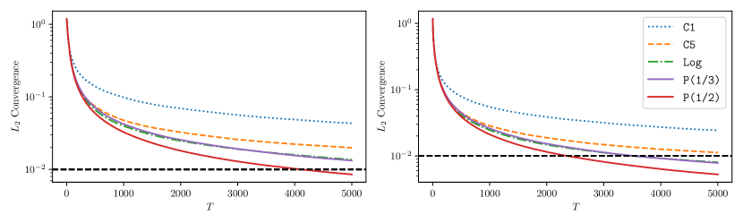
Figure 1: $L_{2}$ convergence $\|\bar{\bm{y}}_{T}-{\bm{x}}^{*}\|$ in terms of communication $T$. Left: Results of linear regression. Right: Results of logistic regression. Black dashed line denotes the nominal coverage rate of 95%.

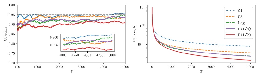
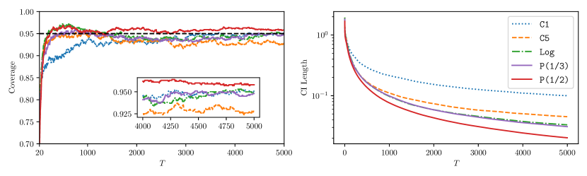
Figure 2: Comparison of the plug-in (the top row) and random scaling (the bottom row) in linear regression. Left: Empirical coverage rate against the number of communication. Black dashed line denotes the nominal coverage rate of 95%. Right: Length of confidence intervals.

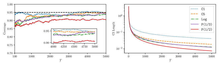
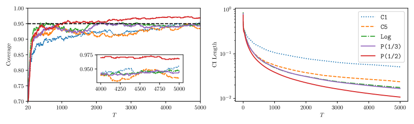
Figure 3: Comparison of the plug-in (the top row) and random scaling (the bottom row) estimators in logistic regression. Left: Empirical coverage rate against the number of communication. Black dashed line denotes the nominal coverage rate of 95%. Right: Length of confidence intervals.

5 Numerical Simulations

This section investigates the empirical performance of the plug-in and random scaling methods via Monte Carlo experiments. We consider both the linear and logistic regression models. At iteration $t$, the $k$-th client observes the pair $(\bm{a}_{t}^{k},b_{t}^{k})$ with $\bm{a}_{t}^{k}$ the $d$-dimensional covariates generated from the multivariate normal distribution ${\mathcal{N}}({\bf 0},{\bf I}_{d})$ and $b_{t}^{k}$ the response generated according to the model. We detail the data generation process as follows:

• In linear regression, $b_{t}^{k}=(\bm{a}_{t}^{k})^{\top}{\bm{x}}_{k}^{*}+\varepsilon_{t}^{k}$ where the $\varepsilon_{t}^{k}$ are i.i.d. according to ${\mathcal{N}}({\bf 0},{\bf I}_{d})$ and ${\bm{x}}_{k}^{*}$ is the true local parameter which we also generate from ${\mathcal{N}}({\bf 0},{\bf I}_{d})$. In this case, the global parameter ${\bm{x}}^{*}$ is the average of ${\bm{x}}_{k}^{*}$’s.

• In logistic regression, $b_{t}^{k}\in\{0,1\}$ is generated to be $1$ with probability $\sigma((\bm{a}_{t}^{k})^{\top}{\bm{x}}^{*})$ and $0$ with probability $1-\sigma((\bm{a}_{t}^{k})^{\top}{\bm{x}}^{*})$. Here $\sigma(\theta)=1/(1+\exp(-\theta))$ is the sigmoid function. We do not impose data heterogeneity for logistic regression in order to avoid numerical error in the calculation of ${\bm{x}}^{*}$. Here ${\bm{x}}^{*}$ is equi-spaced on the interval $[0,1]$ following previous works (Chen et al., 2020; Lee et al., 2021).

We set $\gamma_{m}=\gamma_{0}/m^{0.505}$ with $\gamma_{0}=0.5$ for linear regression and $\gamma_{0}=2$ for logistic regression. The initial value $\bar{\bm{x}}_{0}$ is set as zero. We fix $K=10$ in all our experiments and vary the number of rounds $T$. In all cases, we set $E_{m}=1$ for the first 5% observations as a warm-up and then increase $E_{m}$ from scratch, i.e., $E_{m}=E_{m-5\%*T}^{\prime}$ for another sequence $\{E_{m}^{\prime}\}$. We consider five choices of $\{E_{m}^{\prime}\}_{m}$, namely $(i)$ C1: constant $E_{m}^{\prime}\equiv 1$, $(ii)$ C5: constant $E_{m}^{\prime}\equiv 5$, $(iii)$ Log: logarithmic $E_{m}^{\prime}=\lceil\log_{2}(m+1)\rceil$, $(iv)$ P(1/3): power $E_{m}^{\prime}=\lceil m^{1/3}\rceil$, and $(v)$ P(1/2): power $E_{m}^{\prime}=\lceil m^{1/2}\rceil$. The nominal coverage probability is set at $95\%$. The performance is measured by three statistics: the coverage rate, the average length of the 95% confidence interval, and the average communication frequency. For brevity, we focus on the first coefficient ${\bm{x}}_{1}^{*}$ hereafter. All the reported results are obtained by taking the average of 1000 independent runs.

We first turn to study the communication efficiency for Local SGD. From Figure 1, we find the faster $E_{m}$ grows, the faster the $L_{2}$ convergence in terms of communication, which is consistent with previous studies from optimization perspective (McMahan et al., 2017; Lin et al., 2018). Figure 2 shows the empirical coverage rates and confidence interval lengths in linear regression, both obtained by averaging over 1000 Local SGD paths. The result of logistic regression is depicted in Figure 3. For plug-in, though wandering above $90\%$, the faster $E_{m}$ family (namely, Log, P(1/3) and P(1/2)) has relatively inferior coverage rate than the slower $E_{m}$ family (namely, C1 and C5). For random scaling, it is clear that the coverage rate of all the methods fluctuates around $95\%$. Though with a much smaller deviation from $95\%$, the slow $E_{m}$ family has the slower shrinkage rate for its confidence interval. By contrast, the faster $E_{m}$ family achieves comparable coverage with faster shrinkage of confidence intervals. It implies that Local SGD has high efficiency of communication and maintains a good statistic efficiency via random scaling.

Table 3: Simulation results of linear regression with $d=5$. The standard errors of coverage rates $\widehat{p}$ are computed via $\sqrt{\widehat{p}(1-\widehat{p})/1000}\times 100\%$ and reported inside the parentheses.

Methods	Items		$t_{T}=5000$	$t_{T}=10000$	$t_{T}=20000$	$t_{T}=40000$
Plug-in	Cov Rate (%)	C1	95.70(0.641)	94.20(0.739)	94.20(0.739)	93.80(0.763)
		C5	93.70(0.768)	94.00(0.751)	94.30(0.733)	93.10(0.801)
		Log	91.70(0.872)	93.20(0.796)	93.80(0.763)	93.80(0.763)
		P(1/3)	91.90(0.863)	92.70(0.823)	93.90(0.757)	93.60(0.774)
		P(1/2)	91.10(0.900)	92.60(0.828)	93.90(0.757)	93.80(0.763)
	Avg Len ($10^{-2}$)	C1	7.857(0.099)	5.547(0.050)	3.917(0.025)	2.768(0.013)
		C5	9.737(0.242)	6.868(0.121)	4.847(0.061)	3.423(0.031)
		Log	12.168(0.371)	8.953(0.204)	6.602(0.106)	4.864(0.058)
		P(1/3)	11.372(0.336)	8.656(0.195)	6.613(0.110)	5.059(0.063)
		P(1/2)	15.431(0.559)	12.100(0.327)	9.433(0.188)	7.300(0.112)
Random Scaling	Cov Rate (%)	C1	95.00(0.689)	93.90(0.757)	93.70(0.768)	94.80(0.702)
		C5	97.70(0.474)	96.90(0.548)	97.20(0.522)	96.90(0.548)
		Log	98.20(0.420)	98.70(0.358)	98.90(0.330)	98.80(0.344)
		P(1/3)	97.60(0.484)	98.20(0.420)	98.50(0.384)	98.00(0.443)
		P(1/2)	96.00(0.620)	97.20(0.522)	96.40(0.589)	96.60(0.573)
	Avg Len ($10^{-2}$)	C1	10.011(4.343)	7.081(3.106)	5.010(2.092)	3.605(1.511)
		C5	14.434(6.950)	10.043(4.923)	7.078(3.389)	4.946(2.448)
		Log	19.187(9.763)	14.120(7.154)	10.430(5.219)	7.611(3.895)
		P(1/3)	16.781(8.397)	12.810(6.460)	9.821(4.906)	7.440(3.777)
		P(1/2)	20.888(10.842)	16.127(8.004)	12.379(6.027)	9.314(4.460)

Table 4: Simulation results of logistic regression with $d=5$. The standard errors of coverage rates $\widehat{p}$ are computed via $\sqrt{\widehat{p}(1-\widehat{p})/1000}\times 100\%$ and reported inside the parentheses.

Methods	Items		$t_{T}=5000$	$t_{T}=10000$	$t_{T}=20000$	$t_{T}=40000$
Plug-in	Cov Rate (%)	C1	94.70(0.708)	93.50(0.780)	94.60(0.715)	95.40(0.662)
		C5	93.00(0.807)	92.30(0.843)	93.50(0.780)	94.10(0.745)
		Log	92.30(0.843)	92.10(0.853)	92.60(0.828)	92.90(0.812)
		P(1/3)	92.70(0.823)	92.00(0.858)	92.50(0.833)	92.90(0.812)
		P(1/2)	90.80(0.914)	92.20(0.848)	91.70(0.872)	92.10(0.853)
	Avg Len ($10^{-2}$)	C1	4.113(0.046)	2.903(0.022)	2.049(0.011)	1.448(0.005)
		C5	5.081(0.118)	3.587(0.057)	2.534(0.029)	1.790(0.014)
		Log	6.347(0.175)	4.681(0.093)	3.453(0.049)	2.544(0.027)
		P(1/3)	5.949(0.146)	4.526(0.091)	3.456(0.049)	2.647(0.027)
		P(1/2)	8.062(0.256)	6.320(0.149)	4.927(0.088)	3.821(0.052)
Random Scaling	Cov Rate (%)	C1	95.50(0.656)	92.40(0.838)	94.10(0.745)	94.70(0.708)
		C5	96.00(0.620)	95.90(0.627)	96.80(0.557)	95.80(0.634)
		Log	97.60(0.484)	97.40(0.503)	97.80(0.464)	98.20(0.420)
		P(1/3)	96.10(0.612)	96.60(0.573)	97.50(0.494)	97.90(0.453)
		P(1/2)	94.40(0.727)	94.30(0.733)	94.50(0.721)	95.10(0.683)
	Avg Len ($10^{-2}$)	C1	5.112(2.302)	3.612(1.502)	2.646(1.162)	1.877(0.816)
		C5	7.296(3.714)	5.166(2.535)	3.687(1.836)	2.637(1.316)
		Log	9.703(5.176)	7.241(3.713)	5.383(2.787)	4.023(2.063)
		P(1/3)	8.499(4.465)	6.569(3.345)	5.071(2.621)	3.924(1.999)
		P(1/2)	10.574(5.688)	8.278(4.193)	6.340(3.194)	4.880(2.366)

We then turn to the empirical performance of Local SGD with limited computation or finite samples. Table 3 shows the empirical performance of the five methods under linear models with four different $t_{T}$’s. $t_{T}$ is actually the total iteration each client runs through $T$ rounds or equivalently the number of observations they receive. From the table, all the methods achieve good performance. The random scaling gives better average coverage rates than the plug-in method, because its average coverage rates of all different communication intervals are near (or even exceed) $95\%$. However, its average length is usually larger than that of plug-in. Furthermore, its average length usually has a much larger deviation than that of plug-in. For example, when $t_{T}=5000$, for C5, the standard deviation of average lengths for plug-in is $0.807\times 10^{-2}$, while it increases to $3.714\times 10^{-2}$ for random scaling. Such a wider average length might account for the unexpected advantage on the average coverage rates. However, as the communication round increases and more observations are available, both the average length and its deviations decrease.

In addition, comparing the results of Log, P(1/3), and P(1/2), we can find that the faster $E_{m}$ increases, the larger average length as well as its standard deviations. However, they all have satisfactory performance when observations are sufficient. Indeed, Local SGD trades more computation for less communication, resulting in a residual error gradually accumulated when communication is off, slowing down the convergence rate and enlarging asymptotic variance (e.g., the existence of $\nu$). However, the benefit is also attractive: the averaged communication frequency is substantially reduced and the convergence in terms of communication largely increases. It implies that Local SGD obtains both statistical efficiency and communication efficiency as expected. We further consider the logistic regression, which is a standard non-linear model. The result is given in Table 4. A similar pattern is observed: random scaling has higher average coverage rates at the price of wider average lengths which typically shrink as more observations are generated.

6 Conclusion and Future Work

This paper studies how to perform statistical inference via Local SGD in federated learning. We have established a functional central limit theorem for the averaged iterates of Local SGD and presented two fully online inference methods. We have shown that the Local SGD has statistical efficiency with its asymptotic variance achieving the Cramér–Rao lower bound and communication efficiency with the averaged communication efficiency vanishing asymptotically.

There are many interesting issues for future work. One is to relax the current assumptions and consider Local SGD for more challenging optimization problems (e.g., non-smooth or non-convex problems). Our theory shows that Local SGD enjoys statistical optimality in an asymptotic sense, and it is definitely not also optimal in finite-time convergence (Woodworth et al., 2021). It is then interesting to analyze the statistical properties of other state-of-the-art algorithms in federated learning. For example, Karimireddy et al. (2020) proposed a new algorithm using control variates to remove the effect of data heterogeneity, which achieves a better non-asymptotic convergence rate. It is also interesting to devise more powerful algorithms as well inference methods to handle the challenge in the decentralized big data era (Fan et al., 2021).

Supplementary Material to "Statistical Estimation and Inference via Local SGD in Federated Learning"

Appendix A Proofs for the FCLT

This appendix provides a self-contained proof of Theorem 4.2 as well as the first statement of Theorem 3.1.

A.1 Main Proof

We follows the perturbed iterate framework that is derived by Mania et al. [2017] and widely used in recent works [Stich, 2018, Stich et al., 2018, Li et al., 2019a, Bayoumi et al., 2020, Koloskova et al., 2020, Woodworth et al., 2020a, b]. Then we define a virtual sequence $\bar{\bm{x}}_{t}$ in the following way:

$$\bar{\bm{x}}_{t}=\sum_{k=1}^{K}p_{k}{\bm{x}}_{t}^{k}.$$

Fix a $m\geq 0$ and consider $t_{m}\leq t<t_{m+1}$. Local SGD yields that for any device $k\in[K]$,

$${\bm{x}}_{t+1}^{k} = {\bm{x}}_{t}^{k}-\eta_{m}\nabla f_{k}({\bm{x}}_{t}^{k};\xi_{t}^{k}),$$

$${\bm{x}}_{t_{m+1}}^{k} = \sum_{k=1}^{K}p_{k}\left({\bm{x}}_{t_{m+1}-1}^{k}-\eta_{m}\nabla f_{k}({\bm{x}}_{t_{m+1}-1}^{k};\xi_{t_{m+1}-1}^{k})\right),$$

which implies that we always have

$$\bar{\bm{x}}_{t+1}=\bar{\bm{x}}_{t}-\eta_{m}\bar{\bm{g}}_{t},\quad\text{where}\quad\bar{\bm{g}}_{t}=\sum_{k=1}^{K}p_{k}\nabla f_{k}({\bm{x}}_{t}^{k};\xi_{t}^{k}).$$ (8)

Define ${\bm{s}}_{m}=\bar{\bm{x}}_{t_{m}}-{\bm{x}}^{*}$ and recall that $E_{m}=t_{m+1}-t_{m}$ and $\gamma_{m}=\eta_{m}E_{m}$. Iterating (8) from $t=t_{m}$ to $t_{m+1}-1$ gives

$${\bm{s}}_{m+1}={\bm{s}}_{m}-\eta_{m}\sum_{t=t_{m}}^{t_{m+1}-1}\bar{\bm{g}}_{t}={\bm{s}}_{m}-\gamma_{m}\bm{v}_{m},\quad\text{where}\quad\bm{v}_{m}=\frac{1}{E_{m}}\sum_{t=t_{m}}^{t_{m+1}-1}\bar{\bm{g}}_{t}.$$ (9)

We further decompose $\bm{v}_{m}$ into four terms.

$$\bm{v}_{m} =\bm{G}{\bm{s}}_{m}+\left(\nabla f(\bar{\bm{x}}_{t_{m}})-\bm{G}{\bm{s}}_{m}\right)+(\bm{h}_{m}-\nabla f(\bar{\bm{x}}_{t_{m}}))+(\bm{v}_{m}-\bm{h}_{m})$$

$$:=\bm{G}{\bm{s}}_{m}+\bm{r}_{m}+\bm{{\varepsilon}}_{m}+\bm{\delta}_{m}$$ (10)

where $\bm{G}=\nabla^{2}f({\bm{x}}^{*})$ is the Hessian at the optimum ${\bm{x}}^{*}$ which is non-singular from our assumption, and

$$\bm{h}_{m}=\frac{1}{E_{m}}\sum_{t=t_{m}}^{t_{m+1}-1}\sum_{k=1}^{K}p_{k}\nabla f_{k}(\bar{\bm{x}}_{t_{m}};\xi_{t}^{k}).$$ (11)

Note that $\bm{h}_{m}$ is almost identical to $\bm{v}_{m}$ except that all the stochastic gradients in $\bm{h}_{m}$ are evaluated at $\bar{\bm{x}}_{t_{m}}$ while those in $\bm{v}_{m}$ are evaluated at local variables ${\bm{x}}_{t}^{k}$’s.

Making use of (9) and (10), we have

$${\bm{s}}_{m+1}=(\bm{I}-\gamma_{m}\bm{G}){\bm{s}}_{m}-\gamma_{m}(\bm{r}_{m}+\bm{{\varepsilon}}_{m}+\bm{\delta}_{m}):=\bm{B}_{m}{\bm{s}}_{m}-\gamma_{m}\bm{U}_{m},$$ (12)

where $\bm{B}_{m}:=\bm{I}-\gamma_{m}\bm{G}$ and $\bm{U}_{m}:=\bm{r}_{m}+\bm{{\varepsilon}}_{m}+\bm{\delta}_{m}$ for short. Recurring (12) gives

$${\bm{s}}_{m+1}=\left(\prod_{j=0}^{m}\bm{B}_{j}\right){\bm{s}}_{0}-\sum\limits_{j=0}^{m}\left(\prod\limits_{i=j+1}^{m}\bm{B}_{i}\right)\gamma_{j}\bm{U}_{j}.$$ (13)

Here we use the convention that $\prod\limits_{i=m+1}^{m}\bm{B}_{i}=\bm{I}$ for any $m\geq 0$.

For any $r\in[0,1]$ and $T\geq 1$, define

$$h(r,T)=\max\left\{n\in{\mathbb{Z}}_{+}\bigg{|}r\sum_{m=1}^{T}\frac{1}{E_{m}}\geq\sum_{m=1}^{n}\frac{1}{E_{m}}\right\}.$$ (14)

From Assumption 3.4, we know that $\sum_{m=1}^{T}\frac{1}{E_{m}}\to\infty$ as $T\to\infty$, which implies $h(r,T)\to\infty$ meanwhile. Summing (13) from $m=0$ to $h(r,T)$ gives

$$\frac{\sqrt{t_{T}}}{T}\sum_{m=0}^{h(r,T)}{\bm{s}}_{m+1} =\frac{\sqrt{t_{T}}}{T}\sum_{m=0}^{h(r,T)}\left[\left(\prod_{j=0}^{m}\bm{B}_{j}\right){\bm{s}}_{0}-\sum\limits_{j=0}^{m}\left(\prod\limits_{i=j+1}^{m}\bm{B}_{i}\right)\gamma_{j}\bm{U}_{j}\right]$$

$$=\frac{\sqrt{t_{T}}}{T}\sum_{m=0}^{h(r,T)}\left(\prod_{j=0}^{m}\bm{B}_{j}\right){\bm{s}}_{0}-\frac{\sqrt{t_{T}}}{T}\sum_{j=0}^{h(r,T)}\sum\limits_{m=j}^{h(r,T)}\left(\prod\limits_{i=j+1}^{m}\bm{B}_{i}\right)\gamma_{j}\bm{U}_{j}.$$ (15)

Lemma A.1 (Lemma 1 in Polyak and Juditsky [1992]).

Recall that $\bm{B}_{i}:=\bm{I}-\gamma_{i}\bm{G}$ and $\bm{G}$ is non-singular. For any $n\geq j$, define $\bm{A}_{j}^{n}$ as

$$\bm{A}_{j}^{n}=\sum\limits_{l=j}^{n}\left(\prod\limits_{i=j+1}^{l}\bm{B}_{i}\right)\gamma_{j}.$$ (16)

Under Assumption 3.3, there exists some universal constant $C_{0}>0$ such that for any $n\geq j\geq 0$, $\|\bm{A}_{j}^{n}\|\leq C_{0}$. Furthermore, it follows that $\lim\limits_{n\to\infty}\frac{1}{n}\sum_{j=0}^{n}\|\bm{A}_{j}^{n}-\bm{G}^{-1}\|=0.$

Using the notation of $\bm{A}_{j}^{n}$, we can further simplify (A.1) as

$$\frac{\sqrt{t_{T}}}{T}\sum_{m=0}^{h(r,T)}{\bm{s}}_{m+1}=\frac{\sqrt{t_{T}}}{T\gamma_{0}}\bm{A}_{0}^{h(r,T)}\bm{B}_{0}{\bm{s}}_{0}-\frac{\sqrt{t_{T}}}{T}\sum_{m=0}^{h(r,T)}\bm{A}_{m}^{h(r,T)}\bm{U}_{m}.$$

Since $\bm{U}_{m}=\bm{r}_{m}+\bm{{\varepsilon}}_{m}+\bm{\delta}_{m}$, then

$$\frac{\sqrt{t_{T}}}{T}\sum_{m=0}^{h(r,T)}{\bm{s}}_{m+1}+\frac{\sqrt{t_{T}}}{T}\sum_{m=0}^{h(r,T)}\bm{G}^{-1}\bm{{\varepsilon}}_{m} =\frac{\sqrt{t_{T}}}{T\gamma_{0}}\bm{A}_{0}^{h(r,T)}\bm{B}_{0}{\bm{s}}_{0}-\frac{\sqrt{t_{T}}}{T}\sum_{m=0}^{h(r,T)}\bm{A}_{m}^{h(r,T)}(\bm{r}_{m}+\bm{\delta}_{m})$$

$$\qquad-\frac{\sqrt{t_{T}}}{T}\sum_{m=0}^{h(r,T)}(\bm{A}_{m}^{T}-\bm{G}^{-1})\bm{{\varepsilon}}_{m}$$

$$\qquad-\frac{\sqrt{t_{T}}}{T}\sum_{m=0}^{h(r,T)}(\bm{A}_{m}^{h(r,T)}-\bm{A}_{m}^{T})\bm{{\varepsilon}}_{m}$$

$$:={\mathcal{T}}_{0}-{\mathcal{T}}_{1}-{\mathcal{T}}_{2}-{\mathcal{T}}_{3},$$

where for simplicity we denote

$${\mathcal{T}}_{0}=\frac{\sqrt{t_{T}}}{T\gamma_{0}}\bm{A}_{0}^{h(r,T)}\bm{B}_{0}{\bm{s}}_{0},\quad{\mathcal{T}}_{1}=\frac{\sqrt{t_{T}}}{T}\sum_{m=0}^{h(r,T)}\bm{A}_{m}^{h(r,T)}(\bm{r}_{m}+\bm{\delta}_{m}),$$

$${\mathcal{T}}_{2}=\frac{\sqrt{t_{T}}}{T}\sum_{m=0}^{h(r,T)}(\bm{A}_{m}^{T}-\bm{G}^{-1})\bm{{\varepsilon}}_{m},\quad{\mathcal{T}}_{3}=\frac{\sqrt{t_{T}}}{T}\sum_{m=0}^{h(r,T)}(\bm{A}_{m}^{h(r,T)}-\bm{A}_{m}^{T})\bm{{\varepsilon}}_{m}.$$

With the last equation, we are ready to prove the main theorem which illustrates the partial-sum asymptotic behavior of $\frac{\sqrt{t_{T}}}{T}\sum_{m=0}^{h(r,T)}{\bm{s}}_{m+1}$. The main idea is that we first figure out the partial-sum asymptotic behavior of $\frac{\sqrt{t_{T}}}{T}\sum_{m=0}^{h(r,T)}\bm{G}^{-1}\bm{{\varepsilon}}_{m}$ and then show that their difference is uniformly small, i.e.,

$$\sup_{r\in[0,1]}\left\|\frac{\sqrt{t_{T}}}{T}\sum_{m=0}^{h(r,T)}{\bm{s}}_{m+1}+\frac{\sqrt{t_{T}}}{T}\sum_{m=0}^{h(r,T)}\bm{G}^{-1}\bm{{\varepsilon}}_{m}\right\|=o_{{\mathbb{P}}}(1).$$

For the second step, it suffices to show that the four separate terms: $\sup_{r\in[0,1]}\|{\mathcal{T}}_{0}\|,\sup_{r\in[0,1]}\|{\mathcal{T}}_{1}\|$, $\sup_{r\in[0,1]}\|{\mathcal{T}}_{2}\|$, and $\sup_{r\in[0,1]}\|{\mathcal{T}}_{4}\|$ are $o_{{\mathbb{P}}}(1)$, respectively. With this idea, our following proof is naturally divided into fives parts.

The establishment of almost sure and $L_{2}$ convergence in Lemma A.2 will ease our proof. The following lemma proves the first statement of Theorem 3.1. The second statement of Theorem 3.1 follows directly from Theorem 4.2 which we are going to prove via an argument of the continuous mapping theorem.

Lemma A.2 (Almost sure and $L_{2}$ convergence).

Under Assumptions 3.1, 3.2, and 3.3, $\bar{\bm{x}}_{t_{m}}\to{\bm{x}}^{*}$ almost surely when $m$ goes to infinity. In addition, there exists some $\widetilde{C}_{0}>0$ such that

$${\mathbb{E}}\|\bar{\bm{x}}_{t_{m}}-{\bm{x}}^{*}\|^{2}\leq\widetilde{C}_{0}\gamma_{m}.$$

Part 1: Partial-sum asymptotic behavior of $\frac{\sqrt{t_{T}}}{T}\sum_{m=0}^{h(r,T)}\bm{G}^{-1}\bm{{\varepsilon}}_{m}$.

Lemma A.3.

Under Assumptions 3.1, 3.2, 3.3 and 3.4, the functional martingale CLT holds, namely, for any $r\in[0,1]$,

$$\frac{\sqrt{t_{T}}}{T}\sum_{m=0}^{h(r,T)}\bm{G}^{-1}\bm{{\varepsilon}}_{m}\Rightarrow\sqrt{\nu}\bm{G}^{-1}\bm{S}^{1/2}{\bf B}_{d}(r),$$

where $h(r,T)$ is defined in (14) and ${\bf B}_{d}(r)$ is the $d$-dimensional standard Brownian motion.

Part 2: Uniform negligibility of ${\mathcal{T}}_{0}$.

Lemma A.1 characterizes the asymptotic behavior of $\bm{A}_{j}^{n}$. It is uniformly bounded. It implies

$$\sup_{r\in[0,1]}\|{\mathcal{T}}_{0}\|=\frac{\sqrt{t_{T}}}{T\gamma_{0}}\sup_{r\in[0,1]}\|\bm{A}_{0}^{h(r,T)}\bm{B}_{0}{\bm{s}}_{0}\|\leq\frac{\sqrt{t_{T}}}{T\gamma_{0}}C_{0}\|\bm{B}_{0}{\bm{s}}_{0}\|\to 0,$$

as a result of $\frac{\sqrt{t_{T}}}{T}\to 0$ when $T\to\infty$.

Part 3: Uniform negligibility of ${\mathcal{T}}_{1}$.

The uniform boundedness of $\bm{A}_{j}^{n}$ implies

$$\sup_{r\in[0,1]}\|{\mathcal{T}}_{1}\| =\sup_{r\in[0,1]}\frac{\sqrt{t_{T}}}{T}\left\|\sum_{m=0}^{h(r,T)}\bm{A}_{m}^{h(r,T)}(\bm{r}_{m}+\bm{\delta}_{m})\right\|$$

$$\leq\sup_{r\in[0,1]}\frac{\sqrt{t_{T}}}{T}\sum_{m=0}^{h(r,T)}C_{0}(\|\bm{r}_{m}\|+\|\bm{\delta}_{m}\|)$$

$$=\frac{\sqrt{t_{T}}}{T}\sum_{m=0}^{T}C_{0}(\|\bm{r}_{m}\|+\|\bm{\delta}_{m}\|),$$

where the last inequality uses the fact that $h(r,T)$ increases in $r$ and $h(1,T)=T$. The following two lemmas together imply that $\sup_{r\in[0,1]}\|{\mathcal{T}}_{1}\|=o_{{\mathbb{P}}}(1)$.

Lemma A.4.

Under Assumptions 3.1, 3.2 and 3.3, we have that

$$\frac{\sqrt{t_{T}}}{T}\sum_{m=0}^{T}\left\|\bm{r}_{m}\right\|=o_{{\mathbb{P}}}(1).$$

Lemma A.5.

Under Assumptions 3.1, 3.2 and 3.3, we have that

$$\frac{\sqrt{t_{T}}}{T}\sum_{m=0}^{T}\left\|\bm{\delta}_{m}\right\|=o_{{\mathbb{P}}}(1).$$

Part 4: Uniform negligibility of ${\mathcal{T}}_{2}$.

By Doob’s maximum inequality, it follows that

$${\mathbb{E}}\sup_{r\in[0,1]}\|{\mathcal{T}}_{2}\|^{2} ={\mathbb{E}}\sup_{r\in[0,1]}\frac{t_{T}}{T^{2}}\left\|\sum_{m=0}^{h(r,T)}(\bm{A}_{m}^{T}-\bm{G}^{-1})\bm{{\varepsilon}}_{m}\right\|^{2}$$

$$\leq\frac{t_{T}}{T^{2}}{\mathbb{E}}\left\|\sum_{m=0}^{T}(\bm{A}_{m}^{T}-\bm{G}^{-1})\bm{{\varepsilon}}_{m}\right\|^{2}$$

$$=\frac{t_{T}}{T^{2}}\sum_{m=0}^{T}{\mathbb{E}}\left\|(\bm{A}_{m}^{T}-\bm{G}^{-1})\bm{{\varepsilon}}_{m}\right\|^{2}$$

$$\leq\frac{t_{T}}{T^{2}}\sum_{m=0}^{T}\left\|\bm{A}_{m}^{T}-\bm{G}^{-1}\right\|^{2}{\mathbb{E}}\left\|\bm{{\varepsilon}}_{m}\right\|^{2}.$$

Because $\bm{{\varepsilon}}_{m}=\bm{h}_{m}-\nabla f(\bar{\bm{x}}_{t_{m}})=\frac{1}{E_{m}}\sum_{t=t_{m}}^{t_{m+1}-1}\left(\nabla f(\bar{\bm{x}}_{t_{m}};\xi_{t})-\nabla f(\bar{\bm{x}}_{t_{m}})\right)$ is the mean of $E_{m}$ i.i.d. copies of ${\varepsilon}(\bar{\bm{x}}_{t_{m}}):=\nabla f(\bar{\bm{x}}_{t_{m}};\xi_{t_{m}})-\nabla f(\bar{\bm{x}}_{t_{m}})$ at a fixed $\bar{\bm{x}}_{t_{m}}$, it implies that

$${\mathbb{E}}\left\|\bm{{\varepsilon}}_{m}\right\|^{2}=\frac{1}{E_{m}}{\mathbb{E}}\|{\varepsilon}(\bar{\bm{x}}_{t_{m}})\|^{2}\leq\frac{1}{E_{m}}\left(C_{1}+C_{2}{\mathbb{E}}\|\bar{\bm{x}}_{t_{m}}-{\bm{x}}^{*}\|^{2}\right)\precsim\frac{1}{E_{m}},$$ (17)

where the first inequality is from Lemma A.9 with $C_{1},C_{2}$ two universal constants defined therein and the second inequality uses Lemma A.2. Using the last result, we have that

$${\mathbb{E}}{\mathcal{T}}_{2}\precsim\frac{t_{T}}{T^{2}}\sum_{m=0}^{T}\frac{1}{E_{m}}\left\|\bm{A}_{m}^{T}-\bm{G}^{-1}\right\|^{2}.$$

By Lemma A.1, it follows that as $T\to\infty$,

$$\frac{1}{T}\sum_{m=0}^{T}\left\|\bm{A}_{m}^{T}-\bm{G}^{-1}\right\|^{2}\leq(C_{0}+\|\bm{G}^{-1}\|)\cdot\frac{1}{T}\sum_{m=0}^{T}\left\|\bm{A}_{m}^{T}-\bm{G}^{-1}\right\|\to 0.$$

Lemma A.6 implies that ${\mathbb{E}}\sup_{r\in[0,1]}\|{\mathcal{T}}_{2}\|^{2}=o(1)$.

Lemma A.6.

Let $\{E_{m}\}$ be the positive-integer-valued sequence that satisfies Assumption 3.4. Let $\{a_{m,T}\}_{m\in[T],T\geq 1}$ be a non-negative uniformly bounded sequence satisfying $\lim\limits_{T\to\infty}\frac{1}{T}\sum_{m=0}^{T-1}a_{m,T}=0$. Then

$$\lim\limits_{T\to\infty}\frac{(\sum_{m=0}^{T-1}E_{m})(\sum_{m=0}^{T-1}E_{m}^{-1}a_{m,T})}{T^{2}}=0.$$

Part 5: Uniform negligibility of ${\mathcal{T}}_{3}$.

It is subtle to handle ${\mathcal{T}}_{3}$ because its coefficient depends on $r$.

$$\|{\mathcal{T}}_{3}\| =\frac{\sqrt{t_{T}}}{T}\left\|\sum_{m=0}^{h(r,T)}(\bm{A}_{m}^{T}-\bm{A}_{m}^{h(r,T)})\bm{{\varepsilon}}_{m}\right\|$$

$$=\frac{\sqrt{t_{T}}}{T}\left\|\sum_{m=0}^{h(r,T)}\sum_{l=h(r,T)+1}^{T}\left(\prod\limits_{i=m+1}^{l}\bm{B}_{i}\right)\gamma_{m}\bm{{\varepsilon}}_{m}\right\|$$

$$=\frac{\sqrt{t_{T}}}{T}\left\|\sum_{l=h(r,T)+1}^{T}\sum_{m=0}^{h(r,T)}\left(\prod\limits_{i=m+1}^{l}\bm{B}_{i}\right)\gamma_{m}\bm{{\varepsilon}}_{m}\right\|$$

$$=\frac{\sqrt{t_{T}}}{T}\left\|\sum_{l=h(r,T)+1}^{T}\left(\prod\limits_{i=h(r,T)+1}^{l}\bm{B}_{i}\right)\sum_{m=0}^{h(r,T)}\left(\prod\limits_{i=m+1}^{h(r,T)}\bm{B}_{i}\right)\gamma_{m}\bm{{\varepsilon}}_{m}\right\|$$

$$\precsim\frac{\sqrt{t_{T}}}{T}\left\|\frac{1}{\gamma_{h(r,T)+1}}\sum_{m=0}^{h(r,T)}\left(\prod\limits_{i=m+1}^{h(r,T)}\bm{B}_{i}\right)\gamma_{m}\bm{{\varepsilon}}_{m}\right\|,$$

where the last inequality uses

$$\left\|\sum_{l=h(r,T)+1}^{T}\left(\prod\limits_{i=h(r,T)+1}^{l}\bm{B}_{i}\right)\gamma_{h(r,T)+1}\right\|=\left\|\bm{A}_{h(r,T)+1}^{T}\bm{B}_{h(r,T)+1}\right\|\precsim 1.$$

Lemma A.7 shows that $\sup_{r\in[0,1]}\|{\mathcal{T}}_{3}\|=o_{{\mathbb{P}}}(1)$.

Lemma A.7.

Under Assumptions 3.2 and 3.4, it follows that

$$\sup_{r\in[0,1]}\frac{\sqrt{t_{T}}}{T}\left\|\frac{1}{\gamma_{h(r,T)+1}}\sum_{m=0}^{h(r,T)}\left(\prod\limits_{i=m+1}^{h(r,T)}\bm{B}_{i}\right)\gamma_{m}\bm{{\varepsilon}}_{m}\right\|=o_{{\mathbb{P}}}(1).$$

Remark A.1.

There is a more user-friendly version of Lemma A.7 for a plug-and-play use. Define an auxiliary sequence $\{{\bf Y}_{m}\}_{m\geq 0}$ as following: ${\bf Y}_{0}={\bf 0}$ and for $m\geq 0$,

$${\bf Y}_{m+1}=\bm{B}_{m}{\bf Y}_{m}+\gamma_{m}\bm{{\varepsilon}}_{m}=(\bm{I}-\gamma_{m}\bm{G}){\bf Y}_{m}+\gamma_{m}\bm{{\varepsilon}}_{m}.$$ (18)

It is easy to verify that

$${\bf Y}_{t+1}=\sum_{t=0}^{t}\left(\prod\limits_{i=m+1}^{t}\bm{B}_{i}\right)\gamma_{m}\bm{{\varepsilon}}_{m}.$$

Under this notation, Lemma A.7 is equivalent to

$$\sup_{0\leq t\leq T}\frac{\sqrt{t_{T}}}{T}\frac{\|{\bf Y}_{t+1}\|}{\gamma_{t+1}}=o_{{\mathbb{P}}}(1).$$

More formally, we have the following lemma which one can prove from Lemma A.7.

Lemma A.8.

If the martingale difference sequence $\{\bm{{\varepsilon}}_{m}\}_{m\geq 0}$ satisfies $\sup_{m\geq 0}{\mathbb{E}}\|\bm{{\varepsilon}}_{m}\|^{2+\delta}<\infty$ for some $\delta>0$ and Assumption 3.4 holds with $E_{m}\equiv 1$, for the sequence $\{{\bf Y}_{m}\}_{m\geq 0}$ defined in (18), we have

$$\sup_{0\leq t\leq T}\frac{1}{\sqrt{T}}\frac{\|{\bf Y}_{t+1}\|}{\gamma_{t+1}}=o_{{\mathbb{P}}}(1).$$

A.2 Proof of Lemma A.2

Define ${\mathcal{F}}_{t}=\sigma(\{\xi_{\tau}^{k}\}_{1\leq k\leq K,0\leq\tau<t})$ by the natural filtration generated by $\xi_{\tau}^{k}$’s, so $\{{\bm{x}}_{t}^{k}\}_{t}$ is adapted to $\{{\mathcal{F}}_{t}\}_{t}$ and $\{\bar{\bm{x}}_{t_{m}}\}_{m}$ is adapted to $\{{\mathcal{F}}_{t_{m}}\}_{m}$. Notice that $\bm{v}_{m}=\bm{h}_{m}+\bm{\delta}_{m}$ where

$$\bm{h}_{m}=\frac{1}{E_{m}}\sum_{t=t_{m}}^{t_{m+1}-1}\nabla f(\bar{\bm{x}}_{t_{m}};\xi_{t})\quad\text{and}\quad\nabla f(\bar{\bm{x}}_{t_{m}};\xi_{t})=\sum_{k=1}^{K}p_{k}\nabla f(\bar{\bm{x}}_{t_{m}};\xi_{t}^{k}),$$

implying ${\mathbb{E}}[\bm{h}_{m}|{\mathcal{F}}_{t_{m}}]=\nabla f(\bar{\bm{x}}_{t_{m}})$. The $L$-smoothness of $f(\cdot)$ gives that

$$f(\bar{\bm{x}}_{t_{m+1}}) \leq f(\bar{\bm{x}}_{t_{m}})+\langle\nabla f(\bar{\bm{x}}_{t_{m}}),\bar{\bm{x}}_{t_{m+1}}-\bar{\bm{x}}_{t_{m}}\rangle+\frac{L}{2}\|\bar{\bm{x}}_{t_{m+1}}-\bar{\bm{x}}_{t_{m}}\|^{2}$$

$$=f(\bar{\bm{x}}_{t_{m}})-\gamma_{m}\langle\nabla f(\bar{\bm{x}}_{t_{m}}),\bm{v}_{m}\rangle+\frac{\gamma_{m}^{2}L}{2}\|\bm{v}_{m}\|^{2}.$$

Conditioning on ${\mathcal{F}}_{t_{m}}$ in the last inequality gives

$${\mathbb{E}} [f(\bar{\bm{x}}_{t_{m+1}})|{\mathcal{F}}_{t_{m}}]$$

$$\leq f(\bar{\bm{x}}_{t_{m}})-\gamma_{m}\langle\nabla f(\bar{\bm{x}}_{t_{m}}),{\mathbb{E}}[\bm{v}_{m}|{\mathcal{F}}_{t_{m}}]\rangle+\frac{\gamma_{m}^{2}L}{2}{\mathbb{E}}[\|\bm{v}_{m}\|^{2}|{\mathcal{F}}_{t_{m}}]$$

$$=f(\bar{\bm{x}}_{t_{m}})-\gamma_{m}\|\nabla f(\bar{\bm{x}}_{t_{m}})\|^{2}-\gamma_{m}\langle\nabla f(\bar{\bm{x}}_{t_{m}}),{\mathbb{E}}[\bm{\delta}_{m}|{\mathcal{F}}_{t_{m}}]\rangle+\frac{\gamma_{m}^{2}L}{2}{\mathbb{E}}[\|\bm{h}_{m}+\bm{\delta}_{m}\|^{2}|{\mathcal{F}}_{t_{m}}]$$

$$\leq f(\bar{\bm{x}}_{t_{m}})-\gamma_{m}\|\nabla f(\bar{\bm{x}}_{t_{m}})\|^{2}+\frac{\gamma_{m}}{2}\|\nabla f(\bar{\bm{x}}_{t_{m}})\|^{2}+\frac{\gamma_{m}}{2}\|{\mathbb{E}}[\bm{\delta}_{m}|{\mathcal{F}}_{t_{m}}]\|^{2}$$

$$\qquad\qquad+\gamma_{m}^{2}L{\mathbb{E}}[\|\bm{h}_{m}\|^{2}|{\mathcal{F}}_{t_{m}}]+\gamma_{m}^{2}L{\mathbb{E}}[\|\bm{\delta}_{m}\|^{2}|{\mathcal{F}}_{t_{m}}]$$

$$=f(\bar{\bm{x}}_{t_{m}})-\frac{\gamma_{m}}{2}\|\nabla f(\bar{\bm{x}}_{t_{m}})\|^{2}+\gamma_{m}^{2}L{\mathbb{E}}[\|\bm{h}_{m}\|^{2}|{\mathcal{F}}_{t_{m}}]+\left(\frac{\gamma_{m}}{2}+\gamma_{m}^{2}L\right){\mathbb{E}}[\|\bm{\delta}_{m}\|^{2}|{\mathcal{F}}_{t_{m}}],$$ (19)

where we use the conditional Jensen’s inequality $\|{\mathbb{E}}[\bm{\delta}_{m}|{\mathcal{F}}_{t_{m}}]\|^{2}\leq{\mathbb{E}}[\|\bm{\delta}_{m}\|^{2}|{\mathcal{F}}_{t_{m}}]$.

We then bound the last two terms in the right hand side of (A.2).

Part 1:

For ${\mathbb{E}}[\|\bm{h}_{m}\|^{2}|{\mathcal{F}}_{t_{m}}]$, it follows that

$${\mathbb{E}}[\|\bm{h}_{m}\|^{2}|{\mathcal{F}}_{t_{m}}] =\|{\mathbb{E}}[\bm{h}_{m}|{\mathcal{F}}_{t_{m}}]\|^{2}+{\mathbb{E}}[\|\bm{h}_{m}-{\mathbb{E}}[\bm{h}_{m}|{\mathcal{F}}_{t_{m}}]\|^{2}|{\mathcal{F}}_{t_{m}}]$$

$$=\|\nabla f(\bar{\bm{x}}_{t_{m}})\|^{2}+{\mathbb{E}}[\|\bm{h}_{m}-\nabla f(\bar{\bm{x}}_{t_{m}})\|^{2}|{\mathcal{F}}_{t_{m}}]$$

$$=\|\nabla f(\bar{\bm{x}}_{t_{m}})\|^{2}+\frac{1}{E_{m}}{\mathbb{E}}[\|\nabla f(\bar{\bm{x}}_{t_{m}};\xi_{t_{m}})-\nabla f(\bar{\bm{x}}_{t_{m}})\|^{2}|{\mathcal{F}}_{t_{m}}],$$

where the last equality uses the fact that $\bm{h}_{m}$ is the mean of $E_{m}$ i.i.d. copies of $\nabla f(\bar{\bm{x}}_{t_{m}};\xi_{t_{m}}):=\sum_{k=1}^{K}p_{k}\nabla f_{k}(\bar{\bm{x}}_{t_{m}};\xi_{t_{m}}^{k})$ given ${\mathcal{F}}_{t_{m}}$, so its conditional variance is $E_{m}$ times smaller than the latter,

$${\mathbb{E}}[\|\bm{h}_{m}-\nabla f(\bar{\bm{x}}_{t_{m}})\|^{2}|{\mathcal{F}}_{t_{m}}]=\frac{1}{E_{m}}{\mathbb{E}}[\|\nabla f(\bar{\bm{x}}_{t_{m}};\xi_{t_{m}})-\nabla f(\bar{\bm{x}}_{t_{m}})\|^{2}|{\mathcal{F}}_{t_{m}}].$$ (20)

Lemma A.9.

Recall that ${\varepsilon}(\bar{\bm{x}}_{t_{m}}):=\nabla f(\bar{\bm{x}}_{t_{m}};\xi_{t_{m}})-\nabla f(\bar{\bm{x}}_{t_{m}})$ and ${\varepsilon}_{k}({\bm{x}}_{t}^{k}):=\nabla f({\bm{x}}_{t}^{k};\xi_{t}^{k})-\nabla f({\bm{x}}_{t}^{k})$. Under Assumption 3.2, it follows that

$${\mathbb{E}}_{\xi_{t}^{k}}\|{\varepsilon}_{k}({\bm{x}}_{t}^{k})\|^{2}\leq C_{1}+C_{2}\|{\bm{x}}_{t}^{k}-{\bm{x}}^{*}\|^{2}\quad\text{and}\quad{\mathbb{E}}_{\xi_{t_{m}}}\|{\varepsilon}(\bar{\bm{x}}_{t_{m}})\|^{2}\leq C_{1}+C_{2}\|\bar{\bm{x}}_{t_{m}}-{\bm{x}}^{*}\|^{2}$$

where $C_{1}=d\max_{k\in[K]}\|\bm{S}_{k}\|+\frac{dC}{2}$ and $C_{2}=\frac{3dC}{2}$ with $C$ defined in Assumption 3.2.

With Lemma A.9, we have

$${\mathbb{E}}[\|\nabla f(\bar{\bm{x}}_{t_{m}};\xi_{t_{m}})-\nabla f(\bar{\bm{x}}_{t_{m}})\|^{2}|{\mathcal{F}}_{t_{m}}]\leq C_{1}+C_{2}\|\bar{\bm{x}}_{t_{m}}-{\bm{x}}^{*}\|^{2}.$$

Then, it follows that

$${\mathbb{E}}[\|\bm{h}_{m}\|^{2}|{\mathcal{F}}_{t_{m}}] \leq\|\nabla f(\bar{\bm{x}}_{t_{m}})\|^{2}+\frac{C_{1}}{E_{m}}+\frac{C_{2}}{E_{m}}\|\bar{\bm{x}}_{t_{m}}-{\bm{x}}^{*}\|^{2}.$$

Part 2:

For ${\mathbb{E}}[\|\bm{\delta}_{m}\|^{2}|{\mathcal{F}}_{t_{m}}]$, by Jensen’s inequality, we have

$${\mathbb{E}}[\|\bm{\delta}_{m}\|^{2}|{\mathcal{F}}_{t_{m}}] ={\mathbb{E}}[\|\bm{v}_{m}-\bm{h}_{m}\|^{2}|{\mathcal{F}}_{t_{m}}]$$

$$={\mathbb{E}}\left[\left\|\frac{1}{E_{m}}\sum_{t=t_{m}}^{t_{m+1}-1}\sum_{k=1}^{K}p_{k}\nabla f_{k}({\bm{x}}_{t}^{k};\xi_{t}^{k})-\frac{1}{E_{m}}\sum_{t=t_{m}}^{t_{m+1}-1}\sum_{k=1}^{K}p_{k}\nabla f_{k}(\bar{\bm{x}}_{t_{m}};\xi_{t}^{k})\right\|^{2}\bigg{|}{\mathcal{F}}_{t_{m}}\right]$$

$$\leq\frac{1}{E_{m}}\sum_{t=t_{m}}^{t_{m+1}-1}\sum_{k=1}^{K}p_{k}{\mathbb{E}}\left[\left\|\nabla f_{k}({\bm{x}}_{t}^{k};\xi_{t}^{k})-\nabla f_{k}(\bar{\bm{x}}_{t_{m}};\xi_{t}^{k})\right\|^{2}\big{|}{\mathcal{F}}_{t_{m}}\right].$$

Because ${\bm{x}}_{t}^{k},\bar{\bm{x}}_{t_{m}}\in{\mathcal{F}}_{t}$ and ${\mathcal{F}}_{t_{m}}\subseteq{\mathcal{F}}_{t}$ for $t_{m}\leq t<t_{m+1}$, we have that

$${\mathbb{E}}[\|\nabla f_{k}({\bm{x}}_{t}^{k};\xi_{t}^{k})-\nabla f_{k}(\bar{\bm{x}}_{t_{m}};\xi_{t}^{k})\|^{2}|{\mathcal{F}}_{t_{m}}] ={\mathbb{E}}[{\mathbb{E}}[\|\nabla f_{k}({\bm{x}}_{t}^{k};\xi_{t}^{k})-\nabla f_{k}(\bar{\bm{x}}_{t_{m}};\xi_{t}^{k})\|^{2}|{\mathcal{F}}_{t}]|{\mathcal{F}}_{t_{m}}]$$

$$={\mathbb{E}}[{\mathbb{E}}_{\xi_{t}^{k}}\|\nabla f_{k}({\bm{x}}_{t}^{k};\xi_{t}^{k})-\nabla f_{k}(\bar{\bm{x}}_{t_{m}};\xi_{t}^{k})\|^{2}|{\mathcal{F}}_{t_{m}}]$$

$$\leq L^{2}{\mathbb{E}}[\|{\bm{x}}_{t}^{k}-\bar{\bm{x}}_{t_{m}}\|^{2}|{\mathcal{F}}_{t_{m}}],$$

where the first equality follows from the tower rule of conditional expectation and the second inequality follows from the expected $L$-smoothness in Assumption 3.1.

Combining the last two results, we have

$${\mathbb{E}}[\|\bm{\delta}_{m}\|^{2}|{\mathcal{F}}_{t_{m}}]\leq\frac{L^{2}}{E_{m}}\sum_{t=t_{m}}^{t_{m+1}-1}\sum_{k=1}^{K}p_{k}{\mathbb{E}}[\|{\bm{x}}_{t}^{k}-\bar{\bm{x}}_{t_{m}}\|^{2}|{\mathcal{F}}_{t_{m}}]:=\frac{L^{2}}{E_{m}}\sum_{t=t_{m}}^{t_{m+1}-1}V_{t},$$

where $V_{t}$ is the residual error defined by

$$V_{t}=\sum_{k=1}^{K}p_{k}{\mathbb{E}}[\|{\bm{x}}_{t}^{k}-\bar{\bm{x}}_{t_{m}}\|^{2}|{\mathcal{F}}_{t_{m}}].$$ (21)

The residual error is incurred by multiple local gradient descents. Intuitively, if no local update is used (i.e., $E_{m}=1$), such a residual error would disappear. The following lemma helps us bound $\frac{1}{E_{m}}\sum_{t=t_{m}}^{t_{m+1}-1}V_{t}$ in terms of $\gamma_{m}$ and $\|\bar{\bm{x}}_{t_{m}}-{\bm{x}}^{*}\|^{2}$.

Lemma A.10.

Under Assumptions 3.1 and 3.2, there exist some universal constants $C_{3},C_{4}>0$ such that for any $m$ with $\gamma_{m}^{2}\frac{E_{m}-1}{E_{m}}C_{4}\leq 1$, it follows that

$$\frac{1}{E_{m}}\sum_{t=t_{m}}^{t_{m+1}-1}V_{t}\leq\gamma_{m}^{2}\frac{E_{m}-1}{E_{m}}\left(C_{3}+C_{4}\|\bar{\bm{x}}_{t_{m}}-{\bm{x}}^{*}\|^{2}\right).$$

Almost sure convergence:

Denote $\Delta_{m}=f(\bar{\bm{x}}_{t_{m}})-f({\bm{x}}^{*})$ for simplicity, then from the $\mu$-strongly convexity and $L$-smoothness of $f(\cdot)$, it follows that

$$\frac{\mu}{2}\|\bar{\bm{x}}_{t_{m}}-{\bm{x}}^{*}\|^{2}\leq\Delta_{m}\leq\frac{1}{2\mu}\|\nabla f(\bar{\bm{x}}_{t_{m}})\|^{2}\quad\text{and}\quad\frac{1}{2L}\|\nabla f(\bar{\bm{x}}_{t_{m}})\|^{2}\leq\Delta_{m}\leq\frac{L}{2}\|\bar{\bm{x}}_{t_{m}}-{\bm{x}}^{*}\|^{2}.$$

Note that $\gamma_{m}\to 0$ when $m$ goes to infinity, which means there exists some $m_{0}$, such that for any $m\geq m_{0}$, we have $\gamma_{m}^{2}C_{4}\leq 1$ and $\gamma_{m}\leq\min\{\frac{1}{2L},1\}$. It implies that we can apply Lemma A.10 for sufficiently large $m$. Combining the two parts and plugging them into (A.2) yield for any $m\geq m_{0}$,

$${\mathbb{E}}[\Delta_{m+1}|{\mathcal{F}}_{t_{m}}] \leq\Delta_{m}-\frac{\gamma_{m}}{2}\|\nabla f(\bar{\bm{x}}_{t_{m}})\|^{2}+\gamma_{m}^{2}L\cdot\left[\|\nabla f(\bar{\bm{x}}_{t_{m}})\|^{2}+\frac{C_{1}}{E_{m}}+\frac{C_{2}}{E_{m}}\|\bar{\bm{x}}_{t_{m}}-{\bm{x}}^{*}\|^{2}\right]$$

$$\qquad\qquad+\left(\frac{\gamma_{m}}{2}+\gamma_{m}^{2}L\right)\gamma_{m}^{2}L^{2}\left(C_{3}+C_{4}\|\bar{\bm{x}}_{t_{m}}-{\bm{x}}^{*}\|^{2}\right)$$

$$\leq\Delta_{m}-\gamma_{m}\mu\Delta_{m}+\gamma_{m}^{2}L\cdot\left[\frac{C_{1}}{E_{m}}+\left(2L+\frac{2C_{2}}{\mu E_{m}}\right)\Delta_{m}\right]$$

$$\qquad\qquad+\left(\frac{\gamma_{m}}{2}+\gamma_{m}^{2}L\right)\gamma_{m}^{2}L^{2}\left(C_{3}+\frac{2C_{4}}{\mu}\Delta_{m}\right)$$

$$\leq\Delta_{m}-\gamma_{m}\mu\Delta_{m}+\gamma_{m}^{2}L\cdot\left[C_{1}+\left(2L+\frac{2C_{2}}{\mu}\right)\Delta_{m}\right]+\gamma_{m}^{3}L^{2}\left(C_{3}+\frac{2C_{4}}{\mu}\Delta_{m}\right)$$

$$\leq\Delta_{m}-\gamma_{m}\mu\Delta_{m}+\gamma_{m}^{2}L\cdot\left[C_{1}+\left(2L+\frac{2C_{2}}{\mu}\right)\Delta_{m}\right]+\gamma_{m}^{2}L^{2}\left(C_{3}+\frac{2C_{4}}{\mu}\Delta_{m}\right)$$

$$=\left(1+c_{1}\gamma_{m}^{2}\right)\Delta_{m}+c_{2}\gamma_{m}^{2}-\mu\gamma_{m}\Delta_{m},$$ (22)

where

$$c_{1}=2L^{2}+\frac{2(LC_{2}+L^{2}C_{4})}{\mu}\quad\text{and}\quad c_{2}=LC_{1}+L^{2}C_{3}.$$

To conclude the proof, we need to apply the Robbins-Siegmund theorem [Robbins and Siegmund, 1971].

Lemma A.11 (Robbins-Siegmund theorem).

Let $\{D_{m},\beta_{m},\alpha_{m},\zeta_{m}\}_{m=0}^{\infty}$ be non-negative and adapted to a filtration $\{{\mathcal{G}}_{m}\}_{m=0}^{\infty}$, satisfying

$${\mathbb{E}}[D_{m+1}|{\mathcal{G}}_{m}]\leq(1+\beta_{m})D_{m}+\alpha_{m}-\zeta_{m}$$

for all $m\geq 0$ and both $\sum_{m}\beta_{m}<\infty$ and $\sum_{m}\alpha_{m}<\infty$ almost surely. Then, with probability one, $D_{m}$ converges to a non-negative random variable $D_{\infty}\in[0,\infty)$ and $\sum_{m}\zeta_{m}<\infty$.

From Assumption 3.3, we have that $c_{1}\sum_{m=m_{0}}^{\infty}\gamma_{m}^{2}<\infty$ and $c_{2}\sum_{m=m_{0}}^{\infty}\gamma_{m}^{2}<\infty$. Hence, based on (A.2), Lemma A.11 implies that $\Delta_{m}=f(\bar{\bm{x}}_{t_{m}})-f({\bm{x}}^{*})$ converges to a finite non-negative random variable $\Delta_{\infty}$ almost surely. Moreover, Lemma A.11 also ensures that

$$\mu\sum_{m=m_{0}}^{\infty}\gamma_{m}\Delta_{m}<\infty.$$ (23)

If ${\mathbb{P}}(\Delta_{m}>0)>0$, then the left-hand side of (23) would be infinite with positive probability due to the fact $\sum_{m=m_{0}}^{\infty}\gamma_{m}=\infty$. It reveals that ${\mathbb{P}}(\Delta_{m}=0)=1$ and thus $f(\bar{\bm{x}}_{t_{m}})\to f({\bm{x}}^{*})$ as well as $\bar{\bm{x}}_{t_{m}}\to{\bm{x}}^{*}$ with probability one when $m$ goes to infinity.

$L_{2}$ convergence:

We will obtain the $L_{2}$ convergence rate from (A.2). This part follows the same argument of Su and Zhu [2018] (see Page 37-38 therein). For completeness, we conclude this section by presenting the proof of it. Taking expectation on both sides of (A.2),

$$\frac{{\mathbb{E}}\Delta_{m+1}}{\gamma_{m}}\leq\frac{\gamma_{m-1}\left(1-\mu\gamma_{m}+c_{1}\gamma_{m}^{2}\right)}{\gamma_{m}}\frac{{\mathbb{E}}\Delta_{m}}{\gamma_{m-1}}+c_{2}\gamma_{m}.$$

Because $\gamma_{m}\to 0$, we have that for sufficiently large $m$, $c_{1}\gamma_{m}^{2}\leq 0.5\mu\gamma_{m}$, and hence,

$$\frac{{\mathbb{E}}\Delta_{m+1}}{\gamma_{m}}\leq\frac{\gamma_{m-1}\left(1-\frac{\mu}{2}\gamma_{m}\right)}{\gamma_{m}}\frac{{\mathbb{E}}\Delta_{m}}{\gamma_{m-1}}+c_{2}\gamma_{m}.$$

Lemma A.12 (Lemma A.10 in Su and Zhu [2018]).

Let $c_{1},c_{2}$ be arbitrary positive constants. Assume $\gamma_{m}\to 0$ and $\frac{\gamma_{m-1}}{\gamma_{m}}=1+o(\gamma_{m})$. If $B_{m}>0$ satisfies $B_{m}\leq\frac{\gamma_{m-1}\left(1-c_{1}\gamma_{m}\right)}{\gamma_{m}}B_{m-1}+c_{2}\gamma_{m}$, then $\sup_{m}B_{m}<\infty$.

With the above lemma, we claim that there exists some $C_{5}>0$ such that

$$\sup_{0<m<\infty}\frac{{\mathbb{E}}\Delta_{m}}{\gamma_{m-1}}<C_{5},$$ (24)

which immediately concludes that

$${\mathbb{E}}\|\bar{\bm{x}}_{t_{m}}-{\bm{x}}^{*}\|^{2}\leq\frac{2}{\mu}{\mathbb{E}}\Delta_{m}\leq\frac{2C_{5}}{\mu}\gamma_{m-1}=\frac{2C_{5}}{\mu}(1+o(\gamma_{m}))\gamma_{m}\leq C_{0}\gamma_{m}.$$

A.3 Proof of Lemma A.9

Proof.

By Assumption 3.2, we know that ${\varepsilon}(\bar{\bm{x}}_{t_{m}}):=\nabla f(\bar{\bm{x}}_{t_{m}};\xi_{t_{m}})-\nabla f(\bar{\bm{x}}_{t_{m}})$ satisfies

$$\|{\mathbb{E}}_{\xi_{t_{m}}}{\varepsilon}(\bar{\bm{x}}_{t_{m}}){\varepsilon}(\bar{\bm{x}}_{t_{m}})^{\top}-\bm{S}\|\leq C\left(\|\bar{\bm{x}}_{t_{m}}-{\bm{x}}^{*}\|+\|\bar{\bm{x}}_{t_{m}}-{\bm{x}}^{*}\|^{2}\right).$$

Therefore, it follows that

$${\mathbb{E}}[\|\nabla f(\bar{\bm{x}}_{t_{m}};\xi_{t_{m}})-\nabla f(\bar{\bm{x}}_{t_{m}})\|^{2}|{\mathcal{F}}_{t_{m}}] ={\mathbb{E}}[\|{\varepsilon}(\bar{\bm{x}}_{t_{m}})\|^{2}|{\mathcal{F}}_{t_{m}}]={\mathbb{E}}_{\xi_{t_{m}}}\|{\varepsilon}(\bar{\bm{x}}_{t_{m}})\|^{2}$$

$$=\mathrm{tr}({\mathbb{E}}_{\xi_{t_{m}}}{\varepsilon}(\bar{\bm{x}}_{t_{m}}){\varepsilon}(\bar{\bm{x}}_{t_{m}})^{\top})$$

$$\leq d\|{\mathbb{E}}_{\xi_{t_{m}}}{\varepsilon}(\bar{\bm{x}}_{t_{m}}){\varepsilon}(\bar{\bm{x}}_{t_{m}})^{\top}\|$$

$$\leq d\|\bm{S}\|+dC\|\bar{\bm{x}}_{t_{m}}-{\bm{x}}^{*}\|+dC\|\bar{\bm{x}}_{t_{m}}-{\bm{x}}^{*}\|^{2}$$

$$\leq\left(d\|\bm{S}\|+\frac{dC}{2}\right)+\frac{3dC}{2}\|\bar{\bm{x}}_{t_{m}}-{\bm{x}}^{*}\|^{2}$$

$$\leq C_{1}+C_{2}\|\bar{\bm{x}}_{t_{m}}-{\bm{x}}^{*}\|^{2}$$

with $C_{1}=d\max_{k}\|\bm{S}_{k}\|+\frac{dC}{2}$ and $C_{2}=\frac{3dC}{2}$. Here we use the fact that $\bm{S}=\sum_{k=1}^{K}p_{k}^{2}\bm{S}_{k}$ and thus $\|\bm{S}\|\leq\sum_{k=1}^{K}p_{k}^{2}\|\bm{S}_{k}\|\leq\sum_{k=1}^{K}p_{k}\|\bm{S}_{k}\|\leq\max_{k\in[K]}\|\bm{S}_{k}\|$.

With a similar argument, it follows that

$${\mathbb{E}}_{\xi_{t}^{k}}\|{\varepsilon}_{k}({\bm{x}}_{t}^{k})\|^{2}\leq d\|\bm{S}_{k}\|+\frac{dC}{2}+\frac{3dC}{2}\|{\bm{x}}_{t}^{k}-{\bm{x}}^{*}\|^{2}\leq C_{1}+C_{2}\|{\bm{x}}_{t}^{k}-{\bm{x}}^{*}\|^{2}.$$

∎

A.4 Proof of Lemma A.10

For a fixed $m\geq 0$, let us consider the case where $t_{m+1}>t_{m}+1$, otherwise the result follows directly due to $V_{t_{m}}=0$. For $t_{m}\leq t<t_{m+1}-1$ and $k\in[K]$, we have ${\bm{x}}_{t_{m}}^{k}=\bar{\bm{x}}_{t_{m}}$ and

$${\bm{x}}_{t+1}^{k}={\bm{x}}_{t}^{k}-\eta_{m}\nabla f_{k}({\bm{x}}_{t}^{k};\xi_{t}^{k})\quad\Rightarrow\quad{\bm{x}}_{t+1}^{k}=\bar{\bm{x}}_{t_{m}}-{\color[rgb]{1,0,0}\eta_{m}}\sum_{\tau=t_{m}}^{t}\nabla f_{k}({\bm{x}}_{\tau}^{k};\xi_{\tau}^{k}).$$

Using the last iteration relation, we obtain that

$${\mathbb{E}}[\|{\bm{x}}_{t+1}^{k}-\bar{\bm{x}}_{t_{m}}\|^{2}|{\mathcal{F}}_{t_{m}}] =\eta_{m}^{2}{\mathbb{E}}\left[\left\|\sum_{\tau=t_{m}}^{t}\nabla f_{k}({\bm{x}}_{\tau}^{k};\xi_{\tau}^{k})\right\|^{2}\bigg{|}{\mathcal{F}}_{t_{m}}\right]$$

$$\leq\eta_{m}^{2}(t+1-t_{m})\sum_{\tau=t_{m}}^{t}{\mathbb{E}}[\|\nabla f_{k}({\bm{x}}_{\tau}^{k};\xi_{\tau}^{k})\|^{2}\big{|}{\mathcal{F}}_{t_{m}}]$$

$$\leq\eta_{m}^{2}E_{m}\sum_{\tau=t_{m}}^{t}{\mathbb{E}}[\|\nabla f_{k}({\bm{x}}_{\tau}^{k};\xi_{\tau}^{k})\|^{2}\big{|}{\mathcal{F}}_{t_{m}}]$$

$$=\eta_{m}^{2}E_{m}\sum_{\tau=t_{m}}^{t}{\mathbb{E}}\left[{\mathbb{E}}(\|\nabla f_{k}({\bm{x}}_{\tau}^{k};\xi_{\tau}^{k})\|^{2}\big{|}{\mathcal{F}}_{\tau})\big{|}{\mathcal{F}}_{t_{m}}\right].$$

We then turn to bound ${\mathbb{E}}[\|\nabla f_{k}({\bm{x}}_{\tau}^{k};\xi_{\tau}^{k})\|^{2}\big{|}{\mathcal{F}}_{\tau}]$ as follows:

$${\mathbb{E}}[\|\nabla f_{k}({\bm{x}}_{\tau}^{k};\xi_{\tau}^{k})\|^{2}\big{|}{\mathcal{F}}_{\tau}] ={\mathbb{E}}[\|\nabla f_{k}({\bm{x}}_{\tau}^{k};\xi_{\tau}^{k})-\nabla f_{k}({\bm{x}}_{\tau}^{k})\|^{2}\big{|}{\mathcal{F}}_{\tau}]+\|\nabla f_{k}({\bm{x}}_{\tau}^{k})\|^{2}$$

$$\leq{\mathbb{E}}_{\xi_{\tau}^{k}}\|{\varepsilon}_{k}({\bm{x}}_{\tau}^{k})\|^{2}+2\|\nabla f_{k}({\bm{x}}_{\tau}^{k})-\nabla f_{k}({\bm{x}}^{*})\|^{2}+2\|\nabla f_{k}({\bm{x}}^{*})\|^{2}$$

$$\leq\left(C_{1}+2\|\nabla f_{k}({\bm{x}}^{*})\|^{2}\right)+\left(C_{2}+2L^{2}\right)\|{\bm{x}}_{\tau}^{k}-{\bm{x}}^{*}\|^{2}$$

$$\leq C_{3}+\frac{C_{4}}{2}\|{\bm{x}}_{\tau}^{k}-{\bm{x}}^{*}\|^{2}$$

$$\leq C_{3}+C_{4}\|{\bm{x}}_{\tau}^{k}-\bar{\bm{x}}_{t_{m}}\|^{2}+C_{4}\|\bar{\bm{x}}_{t_{m}}-{\bm{x}}^{*}\|^{2},$$

where $C_{3}=C_{1}+2\max_{k\in[K]}\|\nabla f_{k}({\bm{x}}^{*})\|^{2}$ and $C_{4}=2C_{2}+4L^{2}$. The second inequality uses the $L$-smoothness to bound $\|\nabla f_{k}({\bm{x}}_{\tau}^{k})-\nabla f_{k}({\bm{x}}^{*})\|$ and Lemma A.9 to bound ${\mathbb{E}}_{\xi_{\tau}^{k}}\|{\varepsilon}_{k}({\bm{x}}_{\tau}^{k})\|^{2}$ which yields

$${\mathbb{E}}_{\xi_{\tau}^{k}}\|{\varepsilon}_{k}({\bm{x}}_{\tau}^{k})\|^{2}\leq C_{1}+C_{2}\|{\bm{x}}_{\tau}^{k}-{\bm{x}}^{*}\|^{2}.$$

Therefore, by combing the last two results, we have

$${\mathbb{E}}[\|{\bm{x}}_{t+1}^{k}-\bar{\bm{x}}_{t_{m}}\|^{2}|{\mathcal{F}}_{t_{m}}]\leq\eta_{m}^{2}E_{m}\sum_{\tau=t_{m}}^{t}\left[C_{3}+C_{4}\|\bar{\bm{x}}_{t_{m}}-{\bm{x}}^{*}\|^{2}+C_{4}{\mathbb{E}}[\|{\bm{x}}_{\tau}^{k}-\bar{\bm{x}}_{t_{m}}\|^{2}|{\mathcal{F}}_{t_{m}}]\right].$$

Hence, for $t_{m}\leq t<t_{m+1}-1$, we have

$$V_{t+1}=\sum_{k=1}^{K}p_{k}{\mathbb{E}}(\|{\bm{x}}_{t+1}^{k}-\bar{\bm{x}}_{t_{m}}\|^{2}|{\mathcal{F}}_{t_{m}})\leq\eta_{m}^{2}E_{m}\sum_{\tau=t_{m}}^{t}\left(C_{3}+C_{4}\|\bar{\bm{x}}_{t_{m}}-{\bm{x}}^{*}\|^{2}+C_{4}V_{\tau}\right).$$ (25)

Because $V_{t_{m}}=0$, it then follows that

$$\frac{1}{E_{m}}\sum_{t=t_{m}}^{t_{m+1}-1}V_{t} =\frac{1}{E_{m}}\sum_{t=t_{m}}^{t_{m+1}-2}V_{t+1}$$

$$\leq\eta_{m}^{2}\sum_{t=t_{m}}^{t_{m+1}-2}\sum_{\tau=t_{m}}^{t}\left(C_{3}+C_{4}\|\bar{\bm{x}}_{t_{m}}-{\bm{x}}^{*}\|^{2}+C_{4}V_{\tau}\right)$$

$$=\eta_{m}^{2}\sum_{t=t_{m}}^{t_{m+1}-2}(t_{m+1}-t-1)\left(C_{3}+C_{4}\|\bar{\bm{x}}_{t_{m}}-{\bm{x}}^{*}\|^{2}+C_{4}V_{t}\right)$$

$$\leq\eta_{m}^{2}(E_{m}-1)\sum_{t=t_{m}}^{t_{m+1}-1}\left(C_{3}+C_{4}\|\bar{\bm{x}}_{t_{m}}-{\bm{x}}^{*}\|^{2}+C_{4}V_{t}\right)$$

$$\leq\gamma_{m}^{2}\frac{E_{m}-1}{E_{m}}\left(C_{3}+C_{4}\|\bar{\bm{x}}_{t_{m}}-{\bm{x}}^{*}\|^{2}+\frac{C_{4}}{E_{m}}\sum_{t=t_{m}}^{t_{m+1}-1}V_{t}\right),$$

where we use the definition of $E_{m}=t_{m+1}-t_{m}$ and $\gamma_{m}=\eta_{m}E_{m}$.

Hence, rearranging the last inequality and using the condition $\gamma_{m}^{2}\frac{E_{m}-1}{E_{m}}C_{4}\leq\frac{1}{2}$ gives

$$\frac{1}{E_{m}}\sum_{t=t_{m}}^{t_{m+1}-1}V_{t}\leq 2\gamma_{m}^{2}\frac{E_{m}-1}{E_{m}}\left(C_{3}+C_{4}\|\bar{\bm{x}}_{t_{m}}-{\bm{x}}^{*}\|^{2}\right).$$

Finally redefining $C_{3}:=2C_{3}$ and $C_{4}:=2C_{4}$ completes the proof and the restriction on $\gamma_{m}$ becomes $\gamma_{m}^{2}\frac{E_{m}-1}{E_{m}}C_{4}\leq 1$ under the new notation of $C_{4}$.

A.5 Proof of Lemma A.3

Recall that

$$\bm{{\varepsilon}}_{m}=\bm{h}_{m}-\nabla f(\bar{\bm{x}}_{t_{m}})=\frac{1}{E_{m}}\sum_{t=t_{m}}^{t_{m+1}-1}\left(\nabla f(\bar{\bm{x}}_{t_{m}};\xi_{t})-\nabla f(\bar{\bm{x}}_{t_{m}})\right)$$

where $\nabla f(\bar{\bm{x}}_{t_{m}};\xi_{t})=\sum_{k=1}^{K}p_{k}\nabla f(\bar{\bm{x}}_{t_{m}};\xi_{t}^{k})$ and $\xi_{t}=\{\xi_{t}^{k}\}_{k\in[K]}$, and recall that ${\varepsilon}(\bar{\bm{x}}_{t_{m}})=\nabla f(\bar{\bm{x}}_{t_{m}};\xi_{t_{m}})-\nabla f(\bar{\bm{x}}_{t_{m}})$. Hence $\bm{{\varepsilon}}_{m}$ is the mean of $E_{m}$ i.i.d. copies of ${\varepsilon}(\bar{\bm{x}}_{t_{m}})$ at a fixed $\bar{\bm{x}}_{t_{m}}$.

Define ${\mathcal{F}}_{t}=\sigma(\{\xi_{\tau}^{k}\}_{1\leq k\leq K,0\leq\tau<t})$ by the natural filtration generated by $\xi_{\tau}^{k}$’s and ${\mathcal{G}}_{m-1}={\mathcal{F}}_{t_{m}}$. Then $\{\bm{{\varepsilon}}_{m}\}_{m=1}^{\infty}$ is a martingale difference with respect to $\{{\mathcal{G}}_{m}\}_{m=0}^{\infty}$ (for convention ${\mathcal{G}}_{0}=\{\emptyset,\Omega\}$ if $\bar{\bm{x}}_{0}$ is deterministic, otherwise ${\mathcal{G}}_{0}=\sigma(\bar{\bm{x}}_{0})$): ${\mathbb{E}}[\bm{{\varepsilon}}_{m}|{\mathcal{G}}_{m-1}]={\bf 0}$.

The following lemma establishes an invariance principle which allows us to extend traditional martingale CLT. Interesting readers can find its proof in Hall and Heyde [2014] (see Theorems 4.1, 4.2 and 4.4 therein).

Lemma A.13 (Invariance principles in the martingale CLT).

Let $\{S_{n},{\mathcal{G}}_{n}\}_{n\geq 1}$ be a zero-mean, square-integrable martingale with difference $X_{n}=S_{n}-S_{n-1}(S_{0}=0)$. Let $U_{n}^{2}=\sum_{m=1}^{n}{\mathbb{E}}[X_{m}^{2}|{\mathcal{G}}_{m-1}]$ and $s_{n}^{2}={\mathbb{E}}U_{n}^{2}={\mathbb{E}}S_{n}^{2}$. Define $\zeta_{n}(t)$ as the linear interpolation among the points $(0,0)$, $(U_{n}^{-2}U_{1}^{2},U_{n}^{-1}S_{1})$, $(U_{n}^{-2}U_{2}^{2},U_{n}^{-1}S_{2})$, $\dots$, $(1,U_{n}^{-1}S_{n})$, namely, for $t\in[0,1]$ and $0\leq i\leq n-1$,

$$\zeta_{n}(t):=U_{n}^{-1}\left[S_{i}+(U_{i+1}^{2}-U_{i}^{2})^{-1}(tU_{n}^{2}-U_{i}^{2})X_{i+1}\right]\quad\text{if}\quad U_{i}^{2}\leq tU_{n}^{2}<U_{i+1}^{2}.$$

As $n\to\infty$, if (i) the Linderberg conditions holds, namely for any ${\varepsilon}>0$,

$$s_{n}^{-2}\sum_{m=1}^{n}{\mathbb{E}}[X_{m}^{2}I(|X_{m}|\geq{\varepsilon}s_{n})]\to 0,$$ (26)

and (ii) $s_{n}^{-2}U_{n}^{2}\to 1$ almost surely and $s_{n}^{2}\to\infty$, then

$$\zeta_{n}(t)\Rightarrow B(t)\quad\text{in the sense of}\quad(C,\rho).$$

Here $B(t)$ is the standard Brownian motion on $[0,1]$ and $C=C[0,1]$ is the space of real, continuous functions on $[0,1]$ with the uniform metric $\rho:C[0,1]\to[0,\infty)$, $\rho(\omega)=\max_{t\in[0,1]}|\omega(t)|$.

Lemma A.13 is for univariate martingales. We will use the Cramér-Wold device to reduce the issue of convergence of multivariate martingales to univariate ones. To that end, we fix any uni-norm vector $\bm{a}$ and define $X_{m}=\bm{a}^{\top}\bm{{\varepsilon}}_{m}$. We then check the two conditions in Lemma A.13 hold for such $\{X_{m},{\mathcal{G}}_{m}\}_{m\geq 1}$.

The Linderberg condition:

For one thing, since $\bar{\bm{x}}_{t_{m}}\to{\bm{x}}^{*}$ almost surely from Lemma A.2, we have ${\mathbb{E}}\|{\varepsilon}(\bar{\bm{x}}_{t_{m}})\|^{2+\delta_{2}}\precsim 1$ from Assumption 3.2 when $m$ is sufficiently large.

Lemma A.14 (Marcinkiewicz–Zygmund inequality and Burkholder inequality).

If $Z_{1},\dots,Z_{n}$ are independent random vectors such that ${\mathbb{E}}Z_{m}=0$ and ${\mathbb{E}}|Z_{m}|^{p}<\infty$ for $1\leq p<\infty$, then

$${\mathbb{E}}\left|\frac{1}{n}\sum_{m=1}^{n}Z_{m}\right|^{p}\leq\frac{C_{p}}{n^{\frac{p}{2}}}{\mathbb{E}}\left(\frac{1}{n}\sum_{m=1}^{n}\left|Z_{m}\right|^{2}\right)^{\frac{p}{2}},$$

where the $C_{p}$ are positive constants which depend only on $p$ and not on the underlying distribution of the random variables involved. If $Z_{1},\dots,Z_{n}$ are martingale difference sequence, the above inequality still holds. It is named as Burkholder’s inequality [Dharmadhikari et al., 1968].

Notice that we can rewrite $X_{m}$ as the mean of $E_{m}$ i.i.d. random variables which have the same distribution as $Z_{1}=\bm{a}^{\top}{\varepsilon}(\bar{\bm{x}}_{t_{m}})$: $X_{m}=\frac{1}{E_{m}}\sum_{i=1}^{E_{m}}Z_{i}$. With the Marcinkiewicz–Zygmund inequality and Jensen inequality, it follows that

$${\mathbb{E}}|X_{m}|^{2+\delta_{2}} \precsim E_{m}^{-(1+\frac{\delta_{2}}{2})}{\mathbb{E}}\left(\frac{1}{n}\sum_{m=1}^{n}\left|Z_{m}\right|^{2}\right)^{1+\frac{\delta_{2}}{2}}\precsim E_{m}^{-(1+\frac{\delta_{2}}{2})}{\mathbb{E}}\left|Z_{1}\right|^{2+\delta_{2}}$$

$$\precsim E_{m}^{-(1+\frac{\delta_{2}}{2})}\|\bm{a}\|^{2+\delta_{2}}{\mathbb{E}}\|{\varepsilon}(\bar{\bm{x}}_{t_{m}})\|^{2+\delta_{2}}\precsim E_{m}^{-1}.$$ (27)

Moreover, from Assumption 3.2 and Lemma A.2, we have that

$$\left|{\bm{a}^{\top}\left[{\mathbb{E}}{\varepsilon}(\bar{\bm{x}}_{t_{m}}){\varepsilon}(\bar{\bm{x}}_{t_{m}})^{\top}-\bm{S}\right]\bm{a}}\right| \leq C\left[{\mathbb{E}}\|\bar{\bm{x}}_{t_{m}}-x^{*}\|+{\mathbb{E}}\|\bar{\bm{x}}_{t_{m}}-x^{*}\|^{2}\right]$$

$$\leq C(\sqrt{\gamma_{m}}+\gamma_{m})\to 0.$$

Recall that $\sum_{m=1}^{T}{E_{m}}^{-1}\to\infty$ as $T\to\infty$. The Stolz–Cesàro theorem (Lemma A.15) implies that

$$\lim_{T\to\infty}\frac{s_{T}^{2}}{\sum_{m=1}^{T}\frac{1}{E_{m}}\bm{a}^{\top}\bm{S}\bm{a}}=\lim_{T\to\infty}\frac{\sum_{m=1}^{T}\frac{\bm{a}^{\top}{\mathbb{E}}{\varepsilon}(\bar{\bm{x}}_{t_{m}}){\varepsilon}(\bar{\bm{x}}_{t_{m}})^{\top}\bm{a}}{E_{m}}}{\sum_{m=1}^{T}\frac{1}{E_{m}}\bm{a}^{\top}\bm{S}\bm{a}}=\lim_{T\to\infty}\frac{\bm{a}^{\top}{\mathbb{E}}{\varepsilon}(\bar{\bm{x}}_{t_{T}}){\varepsilon}(\bar{\bm{x}}_{t_{T}})^{\top}\bm{a}}{\bm{a}^{\top}\bm{S}\bm{a}}=1.$$ (28)

Hence, for any ${\varepsilon}>0$, as $T\to\infty$, we have that

$$s_{T}^{-2}\sum_{m=1}^{T}{\mathbb{E}}[X_{m}^{2}I(|X_{m}|\geq{\varepsilon}s_{T})] \leq{\varepsilon}^{-{\delta_{2}}}s_{T}^{-(2+{\delta_{2}})}\sum_{m=1}^{T}{\mathbb{E}}[|X_{m}|^{2+{\delta_{2}}}I(|X_{m}|\geq{\varepsilon}s_{T})]$$

$$\leq{\varepsilon}^{-{\delta_{2}}}s_{T}^{-(2+{\delta_{2}})}\sum_{m=1}^{T}{\mathbb{E}}|X_{m}|^{2+{\delta_{2}}}$$

$$\precsim{\varepsilon}^{-{\delta_{2}}}s_{T}^{-(2+{\delta_{2}})}\sum_{m=1}^{T}\frac{1}{E_{m}}$$

$$\asymp{\varepsilon}^{-{\delta_{2}}}s_{T}^{-{\delta_{2}}}\to 0.$$

The second condition:

We have established the divergence of $\{{\bm{s}}_{T}^{2}\}_{T}$ in (28). Notice that

$$U_{T}^{2} =\sum_{m=1}^{T}{\mathbb{E}}[X_{m}^{2}|{\mathcal{G}}_{m-1}]=\sum_{m=1}^{T}\frac{1}{E_{m}}\bm{a}^{\top}{\mathbb{E}}[{\varepsilon}(\bar{\bm{x}}_{t_{m}}){\varepsilon}(\bar{\bm{x}}_{t_{m}})^{\top}|{\mathcal{G}}_{m-1}]\bm{a}$$

$$=\sum_{m=1}^{T}\frac{1}{E_{m}}\bm{a}^{\top}{\mathbb{E}}_{\xi_{t_{m}}}{\varepsilon}(\bar{\bm{x}}_{t_{m}}){\varepsilon}(\bar{\bm{x}}_{t_{m}})^{\top}\bm{a}.$$

Therefore, from (28) and the Stolz–Cesàro theorem (Lemma A.15), it follows almost surely that

$$\lim_{T\to\infty}\left|\frac{U_{T}^{2}}{s_{T}^{2}}-1\right| \leq\lim_{T\to\infty}\frac{C}{s_{T}^{2}}\sum_{m=1}^{T}\frac{1}{E_{m}}\left[\|\bar{\bm{x}}_{t_{m}}-{\bm{x}}^{*}\|+\|\bar{\bm{x}}_{t_{m}}-{\bm{x}}^{*}\|^{2}\right]$$

$$=\lim_{T\to\infty}\frac{C}{\bm{a}^{\top}\bm{S}\bm{a}}\left[\|\bar{\bm{x}}_{t_{T}}-{\bm{x}}^{*}\|+\|\bar{\bm{x}}_{t_{T}}-{\bm{x}}^{*}\|^{2}\right]\to 0.$$

Lemma A.15 (Stolz–Cesàro theorem).

Let $\{a_{n}\}_{n\geq 1}$ and $\{b_{n}\}_{n\geq 1}$ be two sequences of real numbers. Assume that $\{b_{n}\}_{n\geq 1}$ is a strictly monotone and divergent sequence. We have that

$$\text{if}\ \lim_{n\to\infty}\frac{a_{n+1}-a_{n}}{b_{n+1}-b_{n}}=l,\ \text{then}\ \lim_{n\to\infty}\frac{a_{n}}{b_{n}}=l.$$

We have shown that the two conditions in Lemma A.13 hold. Hence, by definition, $\zeta_{T}(r)\Rightarrow B(r)$ where

$$\zeta_{T}(r):=U_{T}^{-1}\left[S_{i}+(U_{i+1}^{2}-U_{i}^{2})^{-1}(rU_{T}^{2}-U_{i}^{2})X_{i+1}\right]\quad\text{if}\quad U_{i}^{2}\leq rU_{T}^{2}<U_{i+1}^{2}$$

and $S_{i}=\sum_{m=1}^{i}X_{m}$. Since $s_{T}/U_{T}\to 1$ almost surely and (28), it follows that

$$\frac{\sqrt{t_{T}}}{T}U_{T}\zeta_{T}(r)\Rightarrow\sqrt{\nu}\sqrt{\bm{a}^{\top}\bm{S}\bm{a}}B(r)\overset{d.}{=}\sqrt{\nu}\bm{a}^{\top}\bm{S}^{1/2}{\bf B}_{d}(r),$$

where ${\bf B}_{d}(r)$ is the $d$-dimensional standard Brownian motion. Recall that

$$h(r,T)=\max\left\{n\in{\mathbb{Z}}_{+}\bigg{|}r\sum_{m=1}^{T}\frac{1}{E_{m}}\geq\sum_{m=1}^{n}\frac{1}{E_{m}}\right\}.$$

Lemma A.16.

Under the same condition of Lemma A.3, it follows that

$$\sup_{r\in[0,1]}\left|\frac{\sqrt{t_{T}}}{T}U_{T}\zeta_{T}\left(\frac{U_{h(r,T)}^{2}}{U_{T}^{2}}\right)-\frac{\sqrt{t_{T}}}{T}U_{T}\zeta_{T}\left(r\right)\right|\to 0\quad\text{in probability}.$$

Hence,

$$\frac{\sqrt{t_{T}}}{T}\sum_{m=1}^{h(r,T)}\bm{a}^{\top}\bm{{\varepsilon}}_{m}=\frac{\sqrt{t_{T}}}{T}S_{h(r,T)}=\frac{\sqrt{t_{T}}}{T}U_{T}\zeta_{T}\left(\frac{U_{h(r,T)}^{2}}{U_{T}^{2}}\right)\Rightarrow\sqrt{\nu}\bm{a}^{\top}\bm{S}^{1/2}{\bf B}_{d}(r).$$

By the arbitrariness of $\bm{a}$, it follows that

$$\frac{\sqrt{t_{T}}}{T}\sum_{m=1}^{h(r,T)}\bm{{\varepsilon}}_{m}\Rightarrow\sqrt{\nu}\bm{S}^{1/2}{\bf B}_{d}(r).$$

Applying the continuous mapping theorem to the linear function $\bm{{\varepsilon}}:\bm{{\varepsilon}}\mapsto\bm{G}^{-1}\bm{{\varepsilon}}$, we have

$$\frac{\sqrt{t_{T}}}{T}\sum_{m=1}^{h(r,T)}\bm{G}^{-1}\bm{{\varepsilon}}_{m}\Rightarrow\sqrt{\nu}\bm{G}^{-1}\bm{S}^{1/2}{\bf B}_{d}(r).$$

Finally, since ${\mathbb{E}}\frac{\sqrt{t_{T}}}{T}\|\bm{G}^{-1}\bm{{\varepsilon}}_{0}\|\to 0$, it implies that $\frac{\sqrt{t_{T}}}{T}\bm{G}^{-1}\bm{{\varepsilon}}_{0}=o_{{\mathbb{P}}}(1)$. Then it is clear that $\frac{\sqrt{t_{T}}}{T}\sum_{m=0}^{h(r,T)}\bm{G}^{-1}\bm{{\varepsilon}}_{m}\Rightarrow\sqrt{\nu}\bm{G}^{-1}\bm{S}^{1/2}{\bf B}_{d}(r).$

A.6 Proof of Lemma A.16

From the Theorem A.2 of Hall and Heyde [2014], if some random function $\phi_{n}\Rightarrow\phi$ in the sense of $(C,\rho)$, $\{\phi_{n}\}$ must be tight in the sense that for any ${\varepsilon}>0$, ${\mathbb{P}}(\sup_{|s-t|\leq\delta}|\phi_{n}(s)-\phi_{n}(t)|\geq{\varepsilon})\to 0$ uniformly in $n$ as $\delta\to 0$. Since $\frac{\sqrt{t_{T}}}{T}U_{T}\zeta_{T}(r)\Rightarrow\sqrt{\nu}\bm{a}^{\top}\bm{S}^{1/2}{\bf B}_{d}(r)$, $\{\frac{\sqrt{t_{T}}}{T}U_{T}\zeta_{T}\}_{T}$ is tight. We denote the following notation for simplicity

$$\phi_{T}(r)=\frac{\sqrt{t_{T}}}{T}U_{T}\zeta_{T}(r)\quad\text{and}\quad p_{T}(r)=\frac{U_{h(r,T)}^{2}}{U_{T}^{2}}.$$

Since $p_{T}(r)$ satisfies $p_{T}(0)=1-p_{T}(1)=0$ and $p_{T}(r)$ is non-decreasing and right-continuous in $r$, we can view $p_{T}(r)$ as the cumulative distribution function of some random variable on $[0,1]$ and $p(r):r\mapsto r$ is the cumulative distribution function of uniform distribution on $[0,1]$. It is clearly that $p_{T}(r)\to p(r)$ for every $r\in[0,1]$ almost surely, because

$$\lim_{T\to\infty}p_{T}(r)=\lim_{T\to\infty}\frac{U_{h(r,T)}^{2}}{U_{T}^{2}}=\lim_{T\to\infty}\frac{s_{h(r,T)}^{2}}{s_{T}^{2}}=\lim_{T\to\infty}\frac{\sum_{m=1}^{h(r,T)}\frac{1}{E_{m}}}{\sum_{m=1}^{T}\frac{1}{E_{m}}}=r=p(r).$$

Here we use $h(r,T)\to\infty$ for any $r\in[0,1]$ as $T\to\infty$. Since $p(\cdot)$ is additionally continuous, weak convergence implies uniform convergence in cumulative distribution functions, i.e.,

$$\lim_{T\to\infty}\sup_{r\in[0,1]}\left|p_{T}(r)-r\right|=0.$$ (29)

By the tightness of $\{\phi_{n}\}$, for any ${\varepsilon},\eta>0$, we can find a sufficiently small $\delta$ such that

$$\limsup_{T\to\infty}{\mathbb{P}}\left(\sup_{|s-t|\leq\delta}|\phi_{T}(s)-\phi_{T}(t)|\geq{\varepsilon}\right)\leq\eta.$$

With (29), for this $\delta$, ${\mathbb{P}}(\sup_{r\in[0,1]}|p_{T}(r)-r|>\delta)\to 0$ as $T\to\infty$. It implies that

$$\limsup_{T\to\infty}{\mathbb{P}}\left(\sup_{r\in[0,1]}|\phi_{T}\left(p_{T}(r)\right)-\phi_{T}(r)|\geq{\varepsilon}\right)$$

$$\leq \limsup_{T\to\infty}{\mathbb{P}}\left(\sup_{r\in[0,1]}|\phi_{T}\left(p_{T}(r)\right)-\phi_{T}(r)|\geq{\varepsilon},\sup_{r\in[0,1]}|p_{T}(r)-r|\leq\delta\right)$$

$$\qquad+\lim_{T\to\infty}{\mathbb{P}}\left(\sup_{r\in[0,1]}|p_{T}(r)-r|>\delta\right)$$

$$\leq \limsup_{T\to\infty}{\mathbb{P}}\left(\sup_{|s-t|\leq\delta}|\phi_{T}(s)-\phi_{T}(t)|\geq{\varepsilon}\right)\leq\eta.$$

Because $\eta$ is arbitrary, we have shown that

$$\sup_{r\in[0,1]}|\phi_{T}\left(p_{T}(r)\right)-\phi_{T}(r)|\to 0\quad\text{in probability}.$$

A.7 Proof of Lemma A.4

Recall that $\bm{G}=\nabla^{2}f({\bm{x}}^{*}),{\bm{s}}_{m}=\bar{\bm{x}}_{t_{m}}-{\bm{x}}^{*}$ and

$$\bm{r}_{m}=\nabla f(\bar{\bm{x}}_{t_{m}})-\bm{G}{\bm{s}}_{m}.$$

When $\|{\bm{s}}_{m}\|\leq\delta_{1}$, by Assumption 3.1, $\|\nabla^{2}f(s{\bm{s}}_{m}+{\bm{x}}^{*})-\nabla^{2}f({\bm{x}}^{*})\|\leq sL^{\prime}\|{\bm{s}}_{m}\|$, then

$$\|\bm{r}_{m}\| =\|\nabla f({\bm{s}}_{m}+{\bm{x}}^{*})-\nabla f({\bm{x}}^{*})-\nabla^{2}f({\bm{x}}^{*}){\bm{s}}_{m}\|$$

$$=\left\|\int_{0}^{1}\nabla^{2}f(s{\bm{s}}_{m}+{\bm{x}}^{*}){\bm{s}}_{m}ds-\nabla^{2}f({\bm{x}}^{*}){\bm{s}}_{m}\right\|$$

$$\leq\int_{0}^{1}\left\|\nabla^{2}f(s{\bm{s}}_{m}+{\bm{x}}^{*})-\nabla^{2}f({\bm{x}}^{*})\right\|\|{\bm{s}}_{m}\|ds$$

$$\leq\frac{L^{\prime}}{2}\|{\bm{s}}_{m}\|^{2}.$$

When $\|{\bm{s}}_{m}\|>\delta_{1}$, $\|\bm{r}_{m}\|\leq\|\nabla f(\bar{\bm{x}}_{t_{m}})\|+\|\bm{G}{\bm{s}}_{m}\|\leq L\|{\bm{s}}_{m}\|+L\|{\bm{s}}_{m}\|=2L\|{\bm{s}}_{m}\|$. Applying the results above yields

$$\|\bm{r}_{m}\|\leq L^{\prime}\|{\bm{s}}_{m}\|^{2}1_{\{\|{\bm{s}}_{m}\|\leq\delta_{1}\}}+2L\|{\bm{s}}_{m}\|1_{\{\|{\bm{s}}_{m}\|>\delta_{1}\}}.$$

Hence,

$$\frac{\sqrt{t_{T}}}{T}\sum_{m=0}^{T}\left\|\bm{r}_{m}\right\| \leq\frac{\sqrt{t_{T}}}{T}\sum_{m=0}^{T}\left[L^{\prime}\|{\bm{s}}_{m}\|^{2}1_{\{\|{\bm{s}}_{m}\|\leq\delta_{1}\}}+2L\|{\bm{s}}_{m}\|1_{\{\|{\bm{s}}_{m}\|>\delta_{1}\}}\right].$$

By Lemma A.2, ${\bm{s}}_{m}\to 0$ almost surely, which implies

$$\frac{\sqrt{t_{T}}}{T}\sum_{m=0}^{T}\|{\bm{s}}_{m}\|1_{\{\|{\bm{s}}_{m}\|>\delta_{1}\}}\to 0\quad\text{almost surely}.$$

It then suffices to show that $\frac{\sqrt{t_{T}}}{T}\sum_{m=0}^{T}\|{\bm{s}}_{m}\|^{2}1_{\{\|{\bm{s}}_{m}\|\leq\delta_{1}\}}=o_{{\mathbb{P}}}(1)$, which is implied by

$$\frac{\sqrt{t_{T}}}{T}\sum_{m=0}^{T}{\mathbb{E}}\|{\bm{s}}_{m}\|^{2}=o(1).$$

It holds because $\frac{\sqrt{t_{T}}}{T}\sum_{m=0}^{T}{\mathbb{E}}\|{\bm{s}}_{m}\|^{2}\precsim\frac{\sqrt{t_{T}}}{T}\sum_{m=0}^{T}\gamma_{m}\to 0$ from Lemma A.2 and Assumption 3.4.

A.8 Proof of Lemma A.5

In the proof of Lemma A.2 (see the Part 2 therein), we have established for sufficiently large $m$,

$${\mathbb{E}}[\|\bm{\delta}_{m}\|^{2}|{\mathcal{F}}_{t_{m}}]\leq\frac{L^{2}}{E_{m}}\sum_{t=t_{m}}^{t_{m+1}-1}V_{t}\leq L^{2}\gamma_{m}^{2}\frac{E_{m}-1}{E_{m}}\left(C_{3}+C_{4}\|\bar{\bm{x}}_{t_{m}}-{\bm{x}}^{*}\|^{2}\right),$$

where $V_{t}$ is the residual error defined in (21) and $C_{3},C_{4}>0$ are universal constants defined in Lemma A.10. Besides, Lemma A.2 implies that ${\mathbb{E}}\|\bar{\bm{x}}_{t_{m}}-{\bm{x}}^{*}\|^{2}\precsim\gamma_{m}\precsim 1$. It follows that

$${\mathbb{E}}\|\bm{\delta}_{m}\|^{2}\leq L^{2}\gamma_{m}^{2}\left(C_{3}+C_{4}{\mathbb{E}}\|\bar{\bm{x}}_{t_{m}}-{\bm{x}}^{*}\|^{2}\right)\precsim\gamma_{m}^{2}.$$

In order to prove the conclusion, it suffices to show that $\frac{\sqrt{t_{T}}}{T}\sum_{m=0}^{T}{\mathbb{E}}\left\|\bm{\delta}_{m}\right\|\to 0$, which is satisfied because

$$\frac{\sqrt{t_{T}}}{T}\sum_{m=0}^{T}{\mathbb{E}}\left\|\bm{\delta}_{m}\right\|\leq\frac{\sqrt{t_{T}}}{T}\sum_{m=0}^{T}\sqrt{{\mathbb{E}}\left\|\bm{\delta}_{m}\right\|^{2}}\precsim\frac{\sqrt{t_{T}}}{T}\sum_{m=0}^{T}\gamma_{m}\to 0$$

from Lemma A.2 and Assumption 3.4.

A.9 Proof of Lemma A.6

If $\{E_{m}\}$ is uniformly bounded (i.e., there exists some $C$ such that $1\leq E_{m}\leq C$ for all $m$), the conclusion follows because

$$0\leq\frac{(\sum_{m=0}^{T-1}E_{m})(\sum_{m=0}^{T-1}E_{m}^{-1}a_{m,T})}{T^{2}}\leq\frac{CT(\sum_{m=0}^{T-1}a_{m,T})}{T^{2}}=\frac{1}{T}\sum_{m=0}^{T-1}a_{m,T}\to 0\quad\text{when}\quad T\to\infty.$$

In the following, we instead assume $E_{m}$ is non-decreasing in $m$ (i.e., $1\leq E_{m}\leq E_{m+1}$ for all $m$). Let $H_{k}=\sum_{m=0}^{k}a_{m,T}$. For any $\varepsilon$, there exist some $N=N(\varepsilon)$, such that for any $m\geq N$, $0\leq H_{m}\leq m\varepsilon$. Then

$$\sum_{n=N}^{T}\frac{a_{m,T}}{E_{m}} =\sum_{n=N}^{T}\frac{H_{m}-H_{m-1}}{E_{m}}=\frac{H_{T}}{E_{T}}+\sum_{n=N}^{T-1}\left(\frac{1}{E_{m}}-\frac{1}{E_{m+1}}\right)H_{m}-\frac{H_{N-1}}{E_{N}}$$

$$\leq\frac{H_{T}}{E_{T}}+\sum_{n=N}^{T-1}\left(\frac{1}{E_{m}}-\frac{1}{E_{m+1}}\right)m\varepsilon-\frac{H_{N-1}}{E_{N}}$$

$$=\frac{H_{T}-T\varepsilon}{E_{T}}+\left[\frac{T\varepsilon}{E_{T}}+\sum_{n=N}^{T-1}\left(\frac{1}{E_{m}}-\frac{1}{E_{m+1}}\right)m\varepsilon-\frac{(N-1)\varepsilon}{E_{N}}\right]-\frac{H_{N-1}-(N-1)\varepsilon}{E_{N}}$$

$$=\varepsilon\cdot\sum_{n=N}^{T}\frac{1}{E_{m}}+\frac{H_{T}-T\varepsilon}{E_{T}}-\frac{H_{N-1}-(N-1)\varepsilon}{E_{N}}$$

$$\leq\varepsilon\cdot\sum_{n=N}^{T}\frac{1}{E_{m}}+\frac{N\varepsilon}{E_{N}}$$

Recall $t_{T}=\sum_{m=0}^{T-1}E_{m}$. Therefore,

$$\frac{t_{T}(\sum_{m=0}^{T-1}E_{m}^{-1}a_{m,T})}{T^{2}}= \frac{t_{T}(\sum_{m=0}^{N-1}E_{m}^{-1}a_{m,T})}{T^{2}}+\frac{t_{T}(\sum_{m=N}^{T-1}E_{m}^{-1}a_{m,T})}{T^{2}}$$

$$\leq \frac{t_{T}(\sum_{m=0}^{N-1}E_{m}^{-1}a_{m,T})}{T^{2}}+\varepsilon\frac{t_{T}(\sum_{m=N}^{T}E_{m}^{-1})}{T^{2}}+\frac{t_{T}N\varepsilon}{T^{2}E_{N}}.$$

Taking superior limit on both sides and noting $a_{m,T}\precsim 1$ uniformly and $\lim\limits_{T\to\infty}\frac{t_{T}}{T^{2}}=0$, we have

$$0\leq\limsup\limits_{T\to\infty}\frac{t_{T}(\sum_{m=0}^{T-1}E_{m}^{-1}a_{m,T})}{T^{2}}\leq\varepsilon\nu.$$

By the arbitrariness of $\varepsilon$, we complete the proof.

A.10 Proof of Lemma A.7

Without loss of generality, we assume $\bm{G}^{-1}$ is a positive diagonal matrix. Otherwise, we apply the spectrum decomposition to $\bm{G}=\bm{V}{\bf D}\bm{V}^{\top}$ and focus on the coordinates of each $\bm{{\varepsilon}}_{m}$ with respect to the orthogonal base $\bm{V}$. This simplification reduces our multivariate case to a univariate one. Hence, it is enough to show that the result holds for one-dimensional $\bm{{\varepsilon}}_{m}$ and $\bm{G}$. In the following argument, we focus on an eigenvalue $\lambda$ of $\bm{G}$ and its eigenvector $\bm{v}$, and denote ${\varepsilon}_{m}=\bm{v}^{\top}\bm{{\varepsilon}}_{m}$ and $B_{m}=1-\gamma_{m}\lambda\in{\mathbb{R}}$ for simplicity. Clearly, $\lambda\geq 0$ and $0<B_{m}\leq 1$ for sufficiently large $m$.

Given a positive integer $n$, we separate the time interval $[0,T]$ uniformly into $n$ portions with $h_{i}=\left[\frac{iT}{n}\right](i=0,1,\dots,n)$ the $i$-th endpoint. The choice of $n$ is independent of $T$, which implies that $\lim_{T\to\infty}h_{i}=\infty$ for any $i$. Define an event $\mathcal{A}$ whose complement is

$$\mathcal{A}^{c}=\left\{\exists h_{i}\text{ s.t. }\left\|\frac{\sqrt{t_{T}}}{T\gamma_{h_{i}+1}}\sum_{m=0}^{h_{i}}\left(\prod\limits_{i=m+1}^{h_{i}}B_{i}\right)\gamma_{m}{\varepsilon}_{m}\right\|\geq{\varepsilon}\right\}.$$

We claim that $\limsup\limits_{T\to\infty}{\mathbb{P}}({\mathcal{A}}^{c})=0$. Indeed, by the union bound and Markov’s inequality,

$$\mathbb{P}(\mathcal{A}^{c}) \leq\sum_{i=0}^{n}\mathbb{P}\left\{\left\|\frac{\sqrt{t_{T}}}{T\gamma_{h_{i}+1}}\sum_{m=0}^{h_{i}}\prod_{j=m+1}^{h_{i}}B_{j}\gamma_{m}{\varepsilon}_{m}\right\|\geq{\varepsilon}\right\}$$

$$\precsim\sum_{i=0}^{n}\frac{t_{T}}{{\varepsilon}^{2}T^{2}\gamma_{h_{i}+1}^{2}}\sum_{m=0}^{h_{i}}\left(\prod_{j={m+1}}^{h_{i}}B_{j}\right)^{2}\gamma_{m}^{2}$$

$$\precsim\frac{t_{T}}{{\varepsilon}^{2}T^{2}}\sum_{i=0}^{n}\frac{1}{\gamma_{h_{i}+1}}$$

$$\leq\frac{t_{T}(n+1)}{{\varepsilon}^{2}T^{2}\gamma_{T+1}}\to 0\quad\text{as}\quad T\to\infty.$$

Here the last two inequality uses for any $i\in[n]$,

$$\frac{1}{\gamma_{h_{i}+1}}\sum_{m=0}^{h_{i}}\left(\prod_{j={m+1}}^{h_{i}}B_{j}\right)^{2}\gamma_{m}^{2}\precsim 1,$$

which is implied by

$$\lim_{h_{i}\to\infty}\left\{\sum_{m=0}^{h_{i}}\gamma_{m}^{2}\left(\prod_{j=0}^{m}B_{j}\right)^{-2}\right\}\bigg{/}\left\{\gamma_{h_{i}}\left(\prod_{j=0}^{h_{i}}B_{j}\right)^{-2}\right\}$$

$$=\lim_{h_{i}\to\infty}\left\{\gamma_{h_{i}}^{2}\left(\prod_{j=0}^{h_{i}}B_{j}^{-2}\right)\right\}\bigg{/}\left\{o(\gamma_{h_{i}-1})\gamma_{h_{i}-1}\prod_{j=0}^{h_{i}}B_{j}^{-2}+\gamma_{h_{i}}\prod_{j=0}^{h_{i}}B_{j}^{-2}(1-B_{h_{i}}^{2})\right\}$$

$$=\lim_{h_{i}\to\infty}\frac{\gamma_{h_{i}}^{2}}{o(1)\gamma_{h_{i}-1}^{2}+2\lambda\gamma_{h_{i}}^{2}-\lambda^{2}\gamma_{h_{i}}^{3}}$$

$$=\frac{1}{2\lambda}<\infty$$

as a result of the Stolz–Cesàro theorem (Lemma A.15). Here we observe that the denominator $\gamma_{h_{i}}\left(\prod_{j=0}^{h_{i}}B_{j}\right)^{-2}$ increases in $h_{i}$ and diverges when $h_{i}$ is sufficiently large.

Since the event $\mathcal{A}^{c}$ has diminishing probability, we focus on the event $\mathcal{A}$. We will prove that on the event $\mathcal{A}$ our target random sequence is uniformly tight. For notation simplicity, we define

$$X_{m}^{h}=\prod_{i=m}^{h}B_{i}.$$

It follows that

$$\mathbb{P}\left\{\frac{\sqrt{t_{T}}}{T}\sup_{0\leq h\leq T}\left|\frac{1}{\gamma_{h+1}}\sum_{m=0}^{h}\left(\prod_{i=m+1}^{h}B_{i}\right)\gamma_{m}{\varepsilon}_{m}\right|\geq 2{\varepsilon}\text{ ; }\mathcal{A}\right\}$$

$$=\mathbb{P}\left\{\frac{\sqrt{t_{T}}}{T}\sup_{0\leq h\leq T}\left|\frac{1}{\gamma_{h+1}X_{h+1}^{T}}\sum_{m=0}^{h}X_{m+1}^{T}\gamma_{m}{\varepsilon}_{m}\right|\geq 2{\varepsilon}\text{ ; }\mathcal{A}\right\}$$

$$\leq\sum_{i=0}^{n-1}\mathbb{P}\left\{\frac{\sqrt{t_{T}}}{T}\sup_{h\in[h_{i},h_{i+1})}\left|\frac{1}{\gamma_{h+1}X_{h+1}^{T}}\left(\sum_{m=0}^{h}X_{m+1}^{T}\gamma_{m}{\varepsilon}_{m}\right)\right|\geq 2{\varepsilon}\text{ ; }\mathcal{A}\right\}$$

$$\leq\sum_{i=0}^{n-1}\mathbb{P}\left\{\frac{\sqrt{t_{T}}}{T}\sup_{h\in[h_{i},h_{i+1})}\frac{1}{\gamma_{h+1}X_{h+1}^{T}}\left|\sum_{m=0}^{h_{i}}X_{m+1}^{T}\gamma_{m}{\varepsilon}_{m}+\sum_{m=h_{i}+1}^{h}X_{m}^{T}\gamma_{m}{\varepsilon}_{m}\right|\geq 2{\varepsilon}\text{ ; }\mathcal{A}\right\}$$

$$\leq\sum_{i=0}^{n-1}\mathbb{P}\left\{\frac{\sqrt{t_{T}}}{T}\sup_{h\in[h_{i},h_{i+1})}\left[\frac{1}{\gamma_{h+1}X_{h+1}^{T}}\left|\sum_{m=0}^{h_{i}}X_{m+1}^{T}\gamma_{m}{\varepsilon}_{m}\right|+\left|\frac{1}{\gamma_{h}X_{h+1}^{T}}\sum_{m=h_{i}+1}^{h}X_{m}^{T}\gamma_{m}{\varepsilon}_{m}\right|\right]\geq 2{\varepsilon}\text{ ; }\mathcal{A}\right\}$$

$$\leq\sum_{i=0}^{n-1}\mathbb{P}\left\{\frac{\sqrt{t_{T}}}{T}\sup_{h\in[h_{i},h_{i+1})}\left|\frac{1}{\gamma_{h+1}X_{h+1}^{T}}\sum_{m=h_{i}+1}^{h}X_{m+1}^{T}\gamma_{m}{\varepsilon}_{m}\right|\geq{\varepsilon}\text{ ; }\mathcal{A}\right\}$$

$$\leq\sum_{i=0}^{n-1}\mathbb{P}\left\{\frac{\sqrt{t_{T}}}{T}\sup_{h\in[h_{i},h_{i+1})}\left|\frac{1}{\gamma_{h+1}X_{h+1}^{T}}\sum_{m={h_{i}+1}}^{h}X_{m+1}^{T}\gamma_{m}{\varepsilon}_{m}\right|\geq{\varepsilon}\right\}$$

$$=\sum_{i=0}^{n-1}\mathbb{P}\left\{\left(\frac{\sqrt{t_{T}}}{T}\right)^{2+\delta}\sup_{h\in[h_{i},h_{i+1})}\left(\frac{1}{\gamma_{h+1}X_{h+1}^{T}}\right)^{2+\delta}\left|\sum_{m={h_{i}+1}}^{h}X_{m+1}^{T}\gamma_{m}{\varepsilon}_{m}\right|^{2+\delta}\geq{\varepsilon}^{2+\delta}\right\}$$

$$:=\sum_{i=0}^{n-1}\mathcal{P}_{i},$$

where $\delta$ is any positive real number less than $\min\{\delta_{2},\delta_{3}\}$.

Let $Y_{h}=\left|\sum_{m=h_{i}+1}^{h}X_{m+1}^{T}\gamma_{m}{\varepsilon}_{m}\right|^{2+\delta}$. It is clear that $Y_{h}$ is a sub-martingale adapted to the natural filtration. Let $c_{h}=\frac{1}{(\gamma_{h}X_{h}^{T})^{2+\delta}}$. Then $\{c_{h}\}$ is a non-increasing sequence when $h$ is sufficiently large because

$$\gamma_{h}X_{h}^{T}=\frac{\gamma_{h}}{\gamma_{h+1}}(1-\lambda\gamma_{h})\gamma_{h+1}X_{h+1}^{T}=(1+o(\gamma_{h}))(1-\lambda\gamma_{h})\gamma_{h+1}X_{h+1}^{T}\leq\gamma_{h+1}X_{h+1}^{T}$$

for sufficiently large $h$. Indeed, since $h\geq h_{i}=\left[\frac{iT}{n}\right]\to\infty$ as $T\to\infty$, $(1+o(\gamma_{h}))(1-\lambda\gamma_{h})\leq 1$ is solid and $X_{h}^{T}$ is non-negative when $T$ goes to infinity. Hence, each $\mathcal{P}_{i}$ is the probability of the event where the maximum of a sub-martingale multiplied by a non-increasing sequence is larger than a threshold. To bound each $\mathcal{P}_{i}$, we use Chow’s inequality which is a generalization of Doob’s inequality [Chow, 1960]. It follows that

$$\mathcal{P}_{i} =\mathbb{P}\left\{\frac{t_{T}^{1+\delta/2}}{T^{2+\delta}}\sup_{h\in[h_{i},h_{i+1})}c_{h}Y_{h}\geq{\varepsilon}^{2+\delta}\right\}$$

$$\leq\frac{t_{T}^{1+\delta/2}}{{\varepsilon}^{2+\delta}T^{2+\delta}}\left\{c_{h_{i+1}-1}\mathbb{E}Y_{h_{i+1}-1}+\sum_{j=h_{i}+1}^{h_{i+1}-2}(c_{i}-c_{i+1})\mathbb{E}Y_{j}\right\}.$$ (30)

We then apply Burkholder’s inequality to bound each ${\mathbb{E}}Y_{j}$. Burkholder’s inequality is a generalization of the Marcinkiewicz–Zygmund inequality (Lemma A.14) to martingale differences [Dharmadhikari et al., 1968]. That is,

$$\mathbb{E}Y_{j} =\mathbb{E}\left|\sum_{m=h_{i}+1}^{j}X_{m+1}^{T}\gamma_{m}{\varepsilon}_{m}\right|^{2+\delta}$$

$$\precsim(j-h_{i})^{\delta/2}\sum_{m=h_{i}+1}^{j}{\mathbb{E}}\left|X_{m+1}^{T}\gamma_{m}{\varepsilon}_{m}\right|^{2+\delta}$$

$$\precsim(j-h_{i})^{\delta/2}\sum_{m=h_{i}+1}^{j}(X_{m+1}^{T}\gamma_{m})^{2+\delta}/E_{m}^{1+\delta/2}$$

$$\precsim(j-h_{i})^{\delta/2}\sum_{m=h_{i}+1}^{j}c_{m}^{-1}/E_{m}^{1+\delta/2},$$

where we use ${\mathbb{E}}\left|{\varepsilon}_{m}\right|^{2+\delta}\precsim 1/E_{m}^{1+\delta/2}$ for sufficiently large $m$ that is already derived in (A.5).

Plugging it into (A.10) yields that $\mathcal{P}_{i}$ is bounded by

$$\frac{t_{T}^{1+\delta/2}}{{\varepsilon}^{2+\delta}T^{2+\delta}}\left\{c_{h_{i+1}-1}\mathbb{E}Y_{h_{i+1}-1}+\sum_{j=h_{i}+1}^{h_{i+1}-2}(c_{i}-c_{i+1})\mathbb{E}Y_{j}\right\}$$

$$\precsim\frac{t_{T}^{1+\delta/2}}{{\varepsilon}^{2+\delta}T^{2+\delta}}\left\{c_{h_{i+1}{-}1}(h_{i+1}{-}h_{i})^{\frac{\delta}{2}}\sum_{m=h_{i}+1}^{h_{i+1}{-}1}\frac{c_{m}^{-1}}{E_{m}^{1+\delta/2}}+\sum_{j=h_{i}+1}^{h_{i+1}{-}2}(c_{j}{-}c_{j+1})(j{-}h_{i})^{\frac{\delta}{2}}\sum_{m=h_{i}{+}1}^{j}\frac{c_{m}^{-1}}{E_{m}^{1+\delta/2}}\right\}$$

$$\leq\frac{t_{T}^{1+\delta/2}}{{\varepsilon}^{2+\delta}T^{2+\delta}}\left(\frac{T}{n}\right)^{\delta/2}\left\{c_{h_{i+1}-1}\sum_{m=h_{i}+1}^{h_{i+1}-1}\frac{c_{m}^{-1}}{E_{m}^{1+\delta/2}}+\sum_{j=h_{i}+1}^{h_{i+1}-2}(c_{j}-c_{j+1})\sum_{m=h_{i}+1}^{j}\frac{c_{m}^{-1}}{E_{m}^{1+\delta/2}}\right\}$$

$$=\frac{t_{T}^{1+\delta/2}}{{\varepsilon}^{2+\delta}T^{2+\delta}}\left(\frac{T}{n}\right)^{\delta/2}\left\{c_{h_{i+1}-1}\sum_{m=h_{i}+1}^{h_{i+1}-1}\frac{c_{m}^{-1}}{E_{m}^{1+\delta/2}}+\sum_{m=h_{i}+1}^{h_{i+1}-2}(c_{m}-c_{h_{i+1}-1})\frac{c_{m}^{-1}}{E_{m}^{1+\delta/2}}\right\}$$

$$=\frac{t_{T}^{1+\delta/2}}{{\varepsilon}^{2+\delta}T^{2+\delta}}\left(\frac{T}{n}\right)^{\delta/2}\left\{\sum_{m=h_{i}+1}^{h_{i+1}-1}c_{m}\frac{c_{m}^{-1}}{E_{m}^{1+\delta/2}}\right\}$$

$$=\frac{t_{T}^{1+\delta/2}}{{\varepsilon}^{2+\delta}T^{2+\delta}}\left(\frac{T}{n}\right)^{\delta/2}\sum_{m=h_{i}+1}^{h_{i+1}-1}\frac{1}{E_{m}^{1+\delta/2}}.$$

Recall $t_{T}=\sum_{m=0}^{T-1}E_{m}$. Summing the last bound over $i=0,1,\dots,n-1$ gives

$$\sum_{i=0}^{n-1}\mathcal{P}_{i} \precsim\frac{t_{T}^{1+\delta/2}}{{\varepsilon}^{2+\delta}T^{2+\delta}}\left(\frac{T}{n}\right)^{\delta/2}\sum_{m=0}^{T-1}\frac{1}{E_{m}^{1+\delta/2}}$$

$$=\frac{1}{{\varepsilon}^{2+\delta}n^{\delta/2}}\frac{(\frac{1}{T}\sum_{m=0}^{T-1}E_{m})^{1+\delta/2}}{\frac{1}{T}\sum_{m=0}^{T-1}E_{m}^{1+\delta/2}}\frac{\sum_{m=0}^{T-1}E_{m}^{1+\delta/2}\sum_{m=0}^{T-1}1/E_{m}^{1+\delta/2}}{T^{2}}$$

$$\precsim\frac{1}{n^{\delta/2}},$$

where we use $(ii)$ in Assumption 3.4 which implies

$$\sup_{T}\frac{\sum_{m=0}^{T-1}E_{m}^{1+\delta/2}\sum_{m=0}^{T-1}1/E_{m}^{1+\delta/2}}{T^{2}}\leq\sup_{T}\frac{\sum_{m=0}^{T-1}E_{m}^{1+\delta_{3}}\sum_{m=0}^{T-1}1/E_{m}^{1+\delta_{3}}}{T^{2}}<\infty$$

as a result of $\delta<\delta_{3}$.

Summing them all, we have

$$\limsup_{T\to\infty}\mathbb{P}\left\{\frac{\sqrt{t_{T}}}{T}\sup_{0\leq h\leq T}\left|\frac{1}{\gamma_{h+1}}\sum_{m=0}^{h}\left(\prod_{i=m+1}^{h}B_{i}\right)\gamma_{m}{\varepsilon}_{m}\right|\geq 2{\varepsilon}\right\}$$

$$\leq\limsup_{T\to\infty}\mathbb{P}\left\{\frac{\sqrt{t_{T}}}{T}\sup_{0\leq h\leq T}\left|\frac{1}{\gamma_{h+1}}\sum_{m=0}^{h}\left(\prod_{i=m+1}^{h}B_{i}\right)\gamma_{m}{\varepsilon}_{m}\right|\geq 2{\varepsilon}\text{ ; }\mathcal{A}\right\}+\limsup_{T\to\infty}{\mathbb{P}}({\mathcal{A}}^{c})$$

$$\leq\limsup_{T\to\infty}\sum_{i=0}^{n-1}\mathcal{P}_{i}$$

$$\precsim\frac{1}{n^{\delta/2}}.$$

Since the probability of the left hand side has nothing to do with $n$, letting $n\to\infty$ concludes the proof.

Appendix B Proofs of Proposition 3.1

To prove the proposition, we make two following claims.

Claim 1:

For any positive sequences $\{a_{n}\}$ and $\{b_{n}\}$ with $\sum\limits_{n=1}^{T}b_{n}\rightarrow\infty$, we have

$$\limsup\limits_{T\to\infty}\frac{\sum_{n=1}^{T}a_{n}}{\sum_{n=1}^{T}b_{n}}\leq\limsup\limits_{T\to\infty}\frac{a_{T}}{b_{T}}.$$ (31)

Without loss of generality, we assume the right hand side is finite, otherwise (31) follows obviously. We denote that $\limsup\limits_{T\to\infty}\frac{a_{T}}{b_{T}}=\lambda$ for simplicity. Based on the definition of limit superior, for any ${\varepsilon}>0$, there exists $N_{\varepsilon}$ subject to $a_{n}<(\lambda+{\varepsilon})b_{n}$ for $\forall n\geq N_{\varepsilon}$. As a result,

$$\sum\limits_{n=1}^{T}a_{n}=\sum\limits_{n=1}^{N_{\varepsilon}}a_{n}+\sum\limits_{n=N_{\varepsilon}+1}^{T}a_{n}\leq\sum\limits_{n=1}^{N_{\varepsilon}}a_{n}+(\lambda+{\varepsilon})\sum\limits_{n=N_{\varepsilon}+1}^{T}b_{n},$$

which implies

$$\frac{\sum_{n=1}^{T}a_{n}}{\sum_{n=1}^{T}b_{n}}\leq\frac{\sum_{n=1}^{N_{\varepsilon}}a_{n}+(\lambda+{\varepsilon})\sum_{n=N_{\varepsilon}+1}^{T}b_{n}}{\sum_{n=1}^{T}b_{n}}.$$

Taking limit superior on both sides and noting that $\sum\limits_{n=1}^{T}b_{n}\rightarrow\infty$, we have $\frac{\sum_{n=1}^{T}a_{n}}{\sum_{n=1}^{T}b_{n}}\leq\lambda+2{\varepsilon}$. By the arbitrariness of ${\varepsilon}$, (31) follows.

Claim 2:

For any non-decreasing sequence $\{E_{m}\}$ satisfying $\limsup\limits_{T\to\infty}T(1-\frac{E_{T-1}}{E_{T}})<1$, we can find $\delta>0$ such that

$$T\left(\frac{1}{E_{T}}\right)^{1+\delta}-(T-1)\left(\frac{1}{E_{T-1}}\right)^{1+\delta}>0.$$

In fact, we can choose any $\delta<1{-}\limsup\limits_{T\to\infty}T(1{-}\frac{E_{T-1}}{E_{T}})$. In this way, for sufficiently large $T$, we have

$$T\left(\frac{1}{E_{T}}\right)^{1+\delta}-(T-1)\left(\frac{1}{E_{T-1}}\right)^{1+\delta} =\left(\frac{1}{E_{T-1}}\right)^{1+\delta}\left(T\left(\frac{E_{T-1}}{E_{T}}\right)^{1+\delta}-T+1\right)$$

$$\geq T\left(\frac{1}{E_{T-1}}\right)^{1+\delta}\left[\left(1-\frac{1-\delta}{T}\right)^{1+\delta}-1+\frac{1}{T}\right].$$

To lower bound the right hand side, we consider the auxiliary function $h(x)=(1-(1-\delta)x)^{1+\delta}+x$ where $x\in(0,1)$. We claim that $h(x)>1$ for any $x\in(0,1)$. We check it by investigating the derivative of $h(\cdot)$,

$$\dot{h}(x)=-(1+\delta)(1-(1-\delta)x)^{1+\delta}(1-\delta)+1>-(1+\delta)(1-\delta)+1=\delta^{2}>0.$$

Therefore, by mean value theorem, $h(x)>h(0)=1$ which proves the claim.

Now we are well prepared to prove the proposition. It follows that

$$\limsup\limits_{T\to\infty}T\left[1-\left(\frac{E_{T-1}}{E_{T}}\right)^{1+\delta}\right] =\limsup\limits_{T\to\infty}T\frac{(1+\delta)(\theta_{T}E_{T}+(1-\theta_{T})E_{T-1})^{\delta}(E_{T}-E_{T-1})}{E_{T}^{1+\delta}}$$

$$\leq(1+\delta)\limsup\limits_{T\to\infty}\left(\frac{\theta_{T}E_{T}+(1-\theta_{T})E_{T-1}}{E_{T}}\right)^{\delta}\limsup\limits_{T\to\infty}T\frac{E_{T}-E_{T-1}}{E_{T}}$$

$$\leq(1+\delta)(1-\delta)\limsup\limits_{T\to\infty}\left(\frac{\theta_{T}E_{T}+(1-\theta_{T})E_{T-1}}{E_{T}}\right)^{\delta}$$

$$\leq 1-\delta^{2},$$

where the first equality uses mean value theorem with some $\theta_{T}\in[0,1]$.

Therefore,

$$\limsup\limits_{T\to\infty}\frac{(\sum_{m=1}^{T}E_{m}^{1+\delta})(\sum_{m=1}^{T}(1/E_{m})^{1+\delta})}{T^{2}}$$

$$\overset{(a)}{\leq} \limsup\limits_{T\to\infty}\frac{E_{T}^{1+\delta}\sum_{m=1}^{T}(1/E_{m})^{1+\delta}+(\sum_{m=1}^{T}E_{m}^{1+\delta})/(E_{T})^{1+\delta}}{2T-1}$$

$$\leq \limsup\limits_{T\to\infty}\frac{\sum_{m=1}^{T}(1/E_{m})^{1+\delta}}{(2T-1)/E_{T}^{1+\delta}}+\frac{1}{2}$$

$$< \limsup\limits_{T\to\infty}\frac{\sum_{m=1}^{T}(1/E_{m})^{1+\delta}}{T(1/E_{T})^{1+\delta}}$$

$$\overset{(b)}{\leq} \limsup\limits_{T\to\infty}\frac{(1/E_{T})^{1+\delta}}{T(1/E_{T})^{1+\delta}-(T-1)(1/E_{T-1})^{1+\delta}}$$

$$\leq \limsup\limits_{T\to\infty}\frac{1}{1-T\left[1-\left(\frac{E_{T-1}}{E_{T}}\right)^{1+\delta}\right]}$$

$$\leq \left\{1-\limsup\limits_{T\to\infty}T\left[1-\left(\frac{E_{T-1}}{E_{T}}\right)^{1+\delta}\right]\right\}^{-1}\leq\delta^{-2}<\infty,$$

where (a) uses Claim 1 and (b) uses Claim 1 and Claim 2 together.

Furthermore, if the sequence $\{E_{m}\}$ satisfies $\lim\limits_{T\to\infty}T\left(1-\frac{E_{T-1}}{E_{T}}\right)=\rho<1$, then by the Stolz–Cesàro theorem (Lemma A.15), we have

$$\lim\limits_{T\to\infty}\frac{(\sum_{m=1}^{T}E_{m})(\sum_{m=1}^{T}1/E_{m})}{T^{2}}$$

$$= \lim\limits_{T\to\infty}\frac{E_{T}(\sum_{n=1}^{T}1/E_{n})+(\sum_{n=1}^{T-1}E_{n})/E_{T}}{2T-1}$$

$$= \frac{1}{2}\left\{\lim\limits_{T\to\infty}\frac{\sum_{n=1}^{T}1/E_{n}}{T/E_{T}}+\lim\limits_{T\to\infty}\frac{\sum_{n=1}^{T}E_{n}}{TE_{T}}\right\}$$

$$= \frac{1}{2}\left\{\lim\limits_{T\to\infty}\frac{1/E_{T}}{T/E_{T}-(T-1)/E_{T-1}}+\lim\limits_{T\to\infty}\frac{E_{T}}{TE_{T}-(T-1)E_{T-1}}\right\}$$

$$= \frac{1}{2}\left\{\lim\limits_{T\to\infty}\frac{E_{T-1}}{E_{T}}\times\frac{1}{1-T(1-E_{T-1}/E_{T})}+\lim\limits_{T\to\infty}\frac{1}{1+(T-1)(1-E_{T-1}/E_{T})}\right\}$$

$$= \frac{1}{2}\left\{\frac{1}{1-\rho}+\frac{1}{1+\rho}\right\}=\frac{1}{1-\rho^{2}},$$

which completes the proof.

Appendix C Proof for the Plug-in Method, Theorem 4.1

For simplicity, we denote $\nabla f({\bm{x}};\xi_{t})=\sum_{k=1}^{K}p_{k}\nabla f_{k}({\bm{x}};\xi_{t}^{k})$ and $\nabla^{2}f({\bm{x}};\xi_{t})=\sum_{k=1}^{K}p_{k}\nabla^{2}f_{k}({\bm{x}};\xi_{t}^{k})$ where $\xi_{t}=\{\xi_{t}^{k}\}_{k\in[K]}$. We decompose $\widehat{\bm{G}}_{T}-\bm{G}$ into the following terms:

$$\widehat{\bm{G}}_{T}-\bm{G} =\frac{1}{T}\sum_{m=1}^{T}\nabla^{2}f(\bar{\bm{x}}_{t_{m}};\xi_{t_{m}})-\bm{G}$$

$$=\left[\frac{1}{T}\sum_{m=1}^{T}\nabla^{2}f({\bm{x}}^{*};\xi_{t_{m}})-\bm{G}\right]+\frac{1}{T}\sum_{m=1}^{T}\left[\nabla^{2}f(\bar{\bm{x}}_{t_{m}};\xi_{t_{m}})-\nabla^{2}f({\bm{x}}^{*};\xi_{t_{m}})\right].$$ (32)

The first term in (C) is asymptotically zero due to the strong law of large number. With Theorem 3.1, we have known that under the condition, ${\mathbb{E}}\|\bar{\bm{x}}_{t_{m}}-{\bm{x}}^{*}\|\leq\sqrt{{\mathbb{E}}\|\bar{\bm{x}}_{t_{m}}-{\bm{x}}^{*}\|^{2}}\lesssim\sqrt{\gamma_{m}}$. Then the second term in (C) can be bounded via Assumption 4.1

$${\mathbb{E}}\left\|\frac{1}{T}\sum_{m=1}^{T}\left[\nabla^{2}f(\bar{\bm{x}}_{t_{m}};\xi_{t_{m}})-\nabla^{2}f({\bm{x}}^{*};\xi_{t_{m}})\right]\right\| \leq\frac{1}{T}\sum_{m=1}^{T}{\mathbb{E}}\left\|\nabla^{2}f(\bar{\bm{x}}_{t_{m}};\xi_{t_{m}})-\nabla^{2}f({\bm{x}}^{*};\xi_{t_{m}})\right\|$$

$$\leq\frac{L^{\prime\prime}}{T}\sum_{m=1}^{T}{\mathbb{E}}\left\|\bar{\bm{x}}_{t_{m}}-{\bm{x}}^{*}\right\|$$

$$\lesssim\frac{1}{T}\sum_{m=1}^{T}\sqrt{\gamma_{m}}\to 0$$

as $T\to\infty$. Hence, $\widehat{\bm{G}}_{T}$ converges to $\bm{G}$ in probability.

For $\widehat{\bm{S}}_{T}$, note that

$$\nabla f(\bar{\bm{x}}_{t_{m}};\xi_{t_{m}})=\nabla f({\bm{x}}^{*};\xi_{t_{m}})+\left[\nabla f(\bar{\bm{x}}_{t_{m}};\xi_{t_{m}})-\nabla f({\bm{x}}^{*};\xi_{t_{m}})\right]:=\bm{C}_{m}+\bm{D}_{m}.$$

We decompose $\widehat{\bm{S}}_{T}-\bm{S}$ into the following terms:

$$\widehat{\bm{S}}_{T}-\bm{S}=\left(\frac{1}{T}\sum\limits_{m=1}^{T}\bm{C}_{m}\bm{C}_{m}^{\top}-\bm{S}\right)+\frac{1}{T}\sum\limits_{m=1}^{T}\bm{C}_{m}\bm{D}_{m}^{\top}+\frac{1}{T}\sum\limits_{m=1}^{T}\bm{D}_{m}\bm{C}_{m}^{\top}+\frac{1}{T}\sum\limits_{m=1}^{T}\bm{D}_{m}\bm{D}_{m}^{\top}.$$

Because $\{\bm{C}_{m}\}_{m}$ are i.i.d. and ${\mathbb{E}}\bm{C}_{m}\bm{C}_{m}^{\top}=\bm{S}$, the first term is asymptotically zero due to the strong law of large number. Note that ${\mathbb{E}}\|\bm{C}_{m}\|^{2}={\mathbb{E}}\|\bm{C}_{m}\bm{C}_{m}^{\top}\|\leq\mathrm{tr}({\mathbb{E}}\bm{C}_{m}\bm{C}_{m}^{\top})=\mathrm{tr}(\bm{S})$ and

$${\mathbb{E}}\|\bm{D}_{m}\|^{2} ={\mathbb{E}}\left\|\sum_{k=1}^{K}p_{k}\left(\nabla f_{k}(\bar{\bm{x}}_{t_{m}};\xi_{t_{m}}^{k})-\nabla f({\bm{x}}^{*};\xi_{t_{m}}^{k})\right)\right\|^{2}$$

$$\leq\sum_{k=1}^{k}p_{k}{\mathbb{E}}\left\|\nabla f_{k}(\bar{\bm{x}}_{t_{m}};\xi_{t_{m}}^{k})-\nabla f({\bm{x}}^{*};\xi_{t_{m}}^{k})\right\|^{2}$$

$$\leq L^{2}{\mathbb{E}}\|\bar{\bm{x}}_{t_{m}}-{\bm{x}}^{*}\|^{2}\lesssim\gamma_{m}.$$

Then, the second and third terms can be bounded via

$${\mathbb{E}}\left\|\frac{1}{T}\sum\limits_{m=1}^{T}\bm{C}_{m}\bm{D}_{m}^{\top}\right\| \leq\frac{1}{T}\sum\limits_{m=1}^{T}{\mathbb{E}}\|\bm{C}_{m}\|\|\bm{D}_{m}\|$$

$$\leq\frac{1}{T}\sum\limits_{m=1}^{T}\sqrt{{\mathbb{E}}\|\bm{C}_{m}\|^{2}{\mathbb{E}}\|\bm{D}_{m}\|^{2}}$$

$$\lesssim\frac{1}{T}\sum\limits_{m=1}^{T}\sqrt{\gamma_{m}}\to 0.$$

Finally, for the last term, we have that

$${\mathbb{E}}\left\|\frac{1}{T}\sum\limits_{m=1}^{T}\bm{D}_{m}\bm{D}_{m}^{\top}\right\|\leq\frac{1}{T}\sum\limits_{m=1}^{T}{\mathbb{E}}\left\|\bm{D}_{m}\right\|^{2}\lesssim\frac{1}{T}\sum\limits_{m=1}^{T}\gamma_{m}\to 0.$$

Hence, $\widehat{\bm{S}}_{T}$ converges to $\bm{S}$ in probability.

References

- Anastasiou et al. (2019) Andreas Anastasiou, Krishnakumar Balasubramanian, and Murat A Erdogdu. Normal approximation for stochastic gradient descent via non-asymptotic rates of martingale CLT. In Conference on Learning Theory, pages 115–137. PMLR, 2019.
- Bayoumi et al. (2020) Ahmed Khaled Ragab Bayoumi, Konstantin Mishchenko, and Peter Richtárik. Tighter theory for local SGD on identical and heterogeneous data. In International Conference on Artificial Intelligence and Statistics, pages 4519–4529, 2020.
- Blum (1954) Julius R Blum. Approximation methods which converge with probability one. The Annals of Mathematical Statistics, pages 382–386, 1954.
- Chen et al. (2020) Xi Chen, Jason D Lee, Xin T Tong, Yichen Zhang, et al. Statistical inference for model parameters in stochastic gradient descent. The Annals of Statistics, 48(1):251–273, 2020.
- Chen et al. (2021) Xi Chen, Weidong Liu, and Yichen Zhang. First-order newton-type estimator for distributed estimation and inference. Journal of the American Statistical Association, pages 1–40, 2021.
- Chow (1960) YS Chow. A martingale inequality and the law of large numbers. Proceedings of the American Mathematical Society, 11(1):107–111, 1960.
- Dharmadhikari et al. (1968) SW Dharmadhikari, V Fabian, K Jogdeo, et al. Bounds on the moments of martingales. The Annals of Mathematical Statistics, 39(5):1719–1723, 1968.
- Fan et al. (2019) Jianqing Fan, Yongyi Guo, and Kaizheng Wang. Communication-efficient accurate statistical estimation. arXiv preprint arXiv:1906.04870, 2019.
- Fan et al. (2021) Jianqing Fan, Cong Ma, Kaizheng Wang, and Ziwei Zhu. Modern data modeling: Cross-fertilization of the two cultures. Observational Studies, 7(1):65–76, 2021.
- Fang (2019) Yixin Fang. Scalable statistical inference for averaged implicit stochastic gradient descent. Scandinavian Journal of Statistics, 46(4):987–1002, 2019.
- Fang et al. (2018) Yixin Fang, Jinfeng Xu, and Lei Yang. Online bootstrap confidence intervals for the stochastic gradient descent estimator. The Journal of Machine Learning Research, 19(1):3053–3073, 2018.
- Glynn and Whitt (1991) Peter W Glynn and Ward Whitt. Estimating the asymptotic variance with batch means. Operations Research Letters, 10(8):431–435, 1991.
- Haddadpour et al. (2019) Farzin Haddadpour, Mohammad Mahdi Kamani, Mehrdad Mahdavi, and Viveck Cadambe. Local sgd with periodic averaging: Tighter analysis and adaptive synchronization. Advances in Neural Information Processing Systems, 32:11082–11094, 2019.
- Hall and Heyde (2014) Peter Hall and Christopher C Heyde. Martingale limit theory and its application. Academic press, 2014.
- Jordan et al. (2019) Michael I Jordan, Jason D Lee, and Yun Yang. Communication-efficient distributed statistical inference. Journal of the American Statistical Association, 114(526):668–681, 2019.
- Kairouz et al. (2019) Peter Kairouz, H Brendan McMahan, Brendan Avent, Aurélien Bellet, Mehdi Bennis, Arjun Nitin Bhagoji, Keith Bonawitz, Zachary Charles, Graham Cormode, Rachel Cummings, et al. Advances and open problems in federated learning. arXiv preprint arXiv:1912.04977, 2019.
- Karimireddy et al. (2020) Sai Praneeth Karimireddy, Satyen Kale, Mehryar Mohri, Sashank Reddi, Sebastian Stich, and Ananda Theertha Suresh. Scaffold: Stochastic controlled averaging for federated learning. In International Conference on Machine Learning, pages 5132–5143. PMLR, 2020.
- Kiefer et al. (2000) Nicholas M Kiefer, Timothy J Vogelsang, and Helle Bunzel. Simple robust testing of regression hypotheses. Econometrica, 68(3):695–714, 2000.
- Koloskova et al. (2020) Anastasia Koloskova, Nicolas Loizou, Sadra Boreiri, Martin Jaggi, and Sebastian Stich. A unified theory of decentralized SGD with changing topology and local updates. In International Conference on Machine Learning, pages 5381–5393. PMLR, 2020.
- Lee et al. (2021) Sokbae Lee, Yuan Liao, Myung Hwan Seo, and Youngki Shin. Fast and robust online inference with stochastic gradient descent via random scaling. arXiv preprint arXiv:2106.03156v3, 2021.
- Li et al. (2020a) Chris Junchi Li, Wenlong Mou, Martin J Wainwright, and Michael I Jordan. Root-sgd: Sharp nonasymptotics and asymptotic efficiency in a single algorithm. arXiv preprint arXiv:2008.12690, 2020a.
- Li et al. (2020b) Tian Li, Anit Kumar Sahu, Ameet Talwalkar, and Virginia Smith. Federated learning: Challenges, methods, and future directions. IEEE Signal Processing Magazine, 37(3):50–60, 2020b.
- Li et al. (2018) Tianyang Li, Liu Liu, Anastasios Kyrillidis, and Constantine Caramanis. Statistical inference using sgd. In Thirty-Second AAAI Conference on Artificial Intelligence, 2018.
- Li et al. (2019a) Xiang Li, Kaixuan Huang, Wenhao Yang, Shusen Wang, and Zhihua Zhang. On the convergence of FedAvg on non-iid data. In International Conference on Learning Representations, 2019a.
- Li et al. (2019b) Xiang Li, Wenhao Yang, Shusen Wang, and Zhihua Zhang. Communication efficient decentralized training with multiple local updates. arXiv preprint arXiv:1910.09126, 2019b.
- Liang and Su (2019) Tengyuan Liang and Weijie J Su. Statistical inference for the population landscape via moment-adjusted stochastic gradients. Journal of the Royal Statistical Society, 2019.
- Liang et al. (2019) Xianfeng Liang, Shuheng Shen, Jingchang Liu, Zhen Pan, Enhong Chen, and Yifei Cheng. Variance reduced local sgd with lower communication complexity. arXiv preprint arXiv:1912.12844, 2019.
- Lin et al. (2018) Tao Lin, Sebastian U Stich, and Martin Jaggi. Don’t use large mini-batches, use local sgd. arXiv preprint arXiv:1808.07217, 2018.
- Mania et al. (2017) Horia Mania, Xinghao Pan, Dimitris Papailiopoulos, Benjamin Recht, Kannan Ramchandran, and Michael I Jordan. Perturbed iterate analysis for asynchronous stochastic optimization. SIAM Journal on Optimization, 27(4):2202–2229, 2017.
- McMahan et al. (2017) Brendan McMahan, Eider Moore, Daniel Ramage, Seth Hampson, and Blaise Aguera y Arcas. Communication-efficient learning of deep networks from decentralized data. In Artificial Intelligence and Statistics (AISTATS), 2017.
- Mou et al. (2020) Wenlong Mou, Chris Junchi Li, Martin J Wainwright, Peter L Bartlett, and Michael I Jordan. On linear stochastic approximation: Fine-grained polyak-ruppert and non-asymptotic concentration. In Conference on Learning Theory, pages 2947–2997. PMLR, 2020.
- Nishio and Yonetani (2018) Takayuki Nishio and Ryo Yonetani. Client selection for federated learning with heterogeneous resources in mobile edge. arXiv preprint arXiv:1804.08333, 2018.
- Pathak and Wainwright (2020) Reese Pathak and Martin J Wainwright. Fedsplit: an algorithmic framework for fast federated optimization. In Advances in Neural Information Processing Systems, volume 33, pages 7057–7066, 2020.
- Polyak and Juditsky (1992) Boris T Polyak and Anatoli B Juditsky. Acceleration of stochastic approximation by averaging. SIAM journal on control and optimization, 30(4):838–855, 1992.
- Robbins and Siegmund (1971) Herbert Robbins and David Siegmund. A convergence theorem for non negative almost supermartingales and some applications. In Optimizing methods in statistics, pages 233–257. Elsevier, 1971.
- Ruppert (1988) David Ruppert. Efficient estimations from a slowly convergent robbins-monro process. Technical report, Cornell University Operations Research and Industrial Engineering, 1988.
- Sahu et al. (2018) Anit Kumar Sahu, Tian Li, Maziar Sanjabi, Manzil Zaheer, Ameet Talwalkar, and Virginia Smith. Federated optimization for heterogeneous networks. arXiv preprint arXiv:1812.06127, 2018.
- Scott (2015) David W Scott. Multivariate density estimation: theory, practice, and visualization. John Wiley & Sons, 2015.
- Stich (2018) Sebastian U Stich. Local SGD converges fast and communicates little. arXiv preprint arXiv:1805.09767, 2018.
- Stich et al. (2018) Sebastian U Stich, Jean-Baptiste Cordonnier, and Martin Jaggi. Sparsified SGD with memory. In Advances in Neural Information Processing Systems (NIPS), pages 4447–4458, 2018.
- Su and Zhu (2018) Weijie J Su and Yuancheng Zhu. Uncertainty quantification for online learning and stochastic approximation via hierarchical incremental gradient descent. arXiv preprint arXiv:1802.04876, 2018.
- Sun (2014) Yixiao Sun. Let’s fix it: Fixed-b asymptotics versus small-b asymptotics in heteroskedasticity and autocorrelation robust inference. Journal of Econometrics, 178:659–677, 2014.
- Wang and Joshi (2018) Jianyu Wang and Gauri Joshi. Cooperative SGD: A unified framework for the design and analysis of communication-efficient SGD algorithms. arXiv preprint arXiv:1808.07576, 2018.
- Whitt (2002) Ward Whitt. Stochastic-process limits: an introduction to stochastic-process limits and their application to queues. Springer Science & Business Media, 2002.
- Woodworth et al. (2020a) Blake Woodworth, Kumar Kshitij Patel, Sebastian Stich, Zhen Dai, Brian Bullins, Brendan Mcmahan, Ohad Shamir, and Nathan Srebro. Is local SGD better than minibatch SGD? In International Conference on Machine Learning, pages 10334–10343. PMLR, 2020a.
- Woodworth et al. (2021) Blake Woodworth, Brian Bullins, Ohad Shamir, and Nathan Srebro. The min-max complexity of distributed stochastic convex optimization with intermittent communication. arXiv preprint arXiv:2102.01583, 2021.
- Woodworth et al. (2020b) Blake E Woodworth, Kumar Kshitij Patel, and Nati Srebro. Minibatch vs local SGD for heterogeneous distributed learning. In Advances in Neural Information Processing Systems, volume 33, pages 6281–6292, 2020b.
- Yuan and Ma (2020) Honglin Yuan and Tengyu Ma. Federated accelerated stochastic gradient descent. Advances in Neural Information Processing Systems, 33, 2020.
- Yuan et al. (2021) Honglin Yuan, Manzil Zaheer, and Sashank Reddi. Federated composite optimization. In International Conference on Machine Learning, pages 12253–12266. PMLR, 2021.
- Zhang et al. (2020) Xinwei Zhang, Mingyi Hong, Sairaj Dhople, Wotao Yin, and Yang Liu. Fedpd: A federated learning framework with optimal rates and adaptivity to non-iid data. arXiv preprint arXiv:2005.11418, 2020.
- Zhao et al. (2018) Yue Zhao, Meng Li, Liangzhen Lai, Naveen Suda, Damon Civin, and Vikas Chandra. Federated learning with non-iid data. arXiv preprint arXiv:1806.00582, 2018.
- Zheng et al. (2021) Qinqing Zheng, Shuxiao Chen, Qi Long, and Weijie Su. Federated f-differential privacy. In International Conference on Artificial Intelligence and Statistics, pages 2251–2259. PMLR, 2021.
- Zhu et al. (2021) Wanrong Zhu, Xi Chen, and Wei Biao Wu. Online covariance matrix estimation in stochastic gradient descent. Journal of the American Statistical Association, (just-accepted):1–30, 2021.
- Zinkevich et al. (2010) Martin Zinkevich, Markus Weimer, Lihong Li, and Alex J Smola. Parallelized stochastic gradient descent. In Advances in neural information processing systems, pages 2595–2603, 2010.