The SVS13-A Class I chemical complexity as revealed by S-bearing species. SOLIS XIII

Abstract

Context. Recent results in astrochemistry revealed that some molecules such as interstellar complex organic species and deuterated species represent precious tools to investigate star forming regions. Sulphuretted species can also be used to follow the chemical evolution of the early stages of the Sun-like star forming process.

Aims. The goal is to obtain a census of S-bearing species using interferometric images, towards SVS13-A, a Class I object associated with a hot corino rich in interstellar complex organic molecules.

Methods. To this end, we used the NGC1333 SVS13-A data at3mm and 1.4mm obtained with the IRAM-NOEMA interferometer in the framework of the Large Program SOLIS. The line emission of S-bearing species has been imaged and analysed using LTE and LVG approaches.

Results. We imaged the spatial distribution on $\leq$ 300 au scale of the line emission of ³²SO, ³⁴SO, C³²S, C³⁴S, C³³S, OCS, H₂C³²S, H₂C³⁴S, and NS. The low excitation (9 K) ³²SO line is tracing (i) the low-velocity SVS13-A outflow and (ii) the fast (up to 100 km s^-1 away from the systemic velocity) collimated jet driven by the nearby SVS13-B Class 0 object. Conversely, the rest of the lines are confined in the inner SVS13-A region, where complex organics have been previously imaged. More specifically the non-LTE LVG analysis of SO, SO₂, and H₂CS indicates a hot corino origin (size in the 60-120 au range). Temperatures between 50 K and 300 K, and volume densities larger than 10⁵ cm^-3 have been derived. The abundances of the sulphuretted are in the following ranges: 0.3–6 $\times$ 10^-6 (CS), 7 $\times$ 10^-9 – 1 $\times$ 10^-7 (SO), 1–10 $\times$ 10^-7 (SO₂), a few 10^-10 (H₂CS and OCS), and 10^-10–10^-9 (NS). The N(NS)/N(NS⁺) ratio is larger than 10, supporting that the NS⁺ ion is mainly formed in the extended envelope.

Conclusions. The [H₂CS]/[H₂CO] ratio, once measured at high-spatial resolutions, increases with time (from Class 0 to Class II objects) by more than one order of magnitude (from $\leq$ 10^-2 to a few 10^-1). This suggests that [S]/[O] changes along the Sun-like star forming process. Finally, the estimate of the [S]/[H] budget in SVS13-A is 2%-17% of the Solar System value (1.8 $\times$ 10^-5), being consistent with what was previously measured towards Class 0 objects (1%-8%). This supports that the enrichment of the sulphuretted species with respect to dark clouds keeps constant from the Class 0 to the Class I stages of low-mass star formation. The present findings stress the importance of investigating the chemistry of star forming regions using large observational surveys as well as sampling regions on a Solar System scale.

1 Introduction

Molecular complexity builds up at each step of the process leading to Sun-like star formation. Searches for exoplanets have shown a large degree of diversity in the planetary systems, and it is unclear how common a System like our own is. In this context, the role of the pre-solar chemistry in the formation of the Solar System bodies is far from being understood. A breakthrough question (see e.g. Ceccarelli et al., 2007; Herbst & van Dishoeck, 2009; Caselli & Ceccarelli, 2012; Jørgensen et al., 2020, and references therein) is to understand whether planetary systems inherited at least part of the chemical composition of the earliest stages of the Sun-like star forming process, such as prestellar cloud, Class 0 ($\leq$ 10⁵ yr), Class I ($>$ 10⁵ yr), and Class II ($>$ 10⁶ yr) objects. To progress, it is of paramount importance: (i) to observe objects representing all the evolutionary stages of the star forming process sampling regions on a Solar System scale, and (ii) to combine high-sensitivity spectral surveys collecting a large number of species and emitting lines to constrain their abundances.

In the last years, ALMA revolutionised our comprehension of planet formation, delivering images of rings and gaps (see e.g., Sheehan & Eisner, 2017; Fedele et al., 2018; Andrews et al., 2018) in the dust distribution around objects with an age less than 1 Myr. This clearly supports that planet formation occurs earlier than what was postulated before, more specifically already in the Class I phase. This in turn stresses the importance of investigating Class I objects, a sort of bridge between the prototellar phase and the protoplanetary disks around Class II young objects. Several projects focused on the chemical complexity of Class I objects have been recently performed, mainly focusing the attention on interstellar small or complex (with at least 6 atom) organic molecules and/or deuteration using both single-dishes and interferometer (see e.g., Öberg et al., 2014; Bianchi et al., 2017; Bergner et al., 2017, 2019; Bianchi et al., 2019a, b, 2020; Le Gal et al., 2020; Yang et al., 2021).

In the dense gas typical of star forming regions, [S]/[H] is far to the value measured in our Solar System (1.8 $\times$ 10^-5 Anders & Grevesse, 1989), given sulphur is depleted by several orders of magnitude (e.g. Tieftrunk et al., 1994; Wakelam et al., 2004a; Phuong et al., 2018; Laas & Caselli, 2019; van ’t Hoff et al., 2020). On grains, sulphur is expected to be very refractory, likely in the form of FeS (Kama et al., 2019) or S₈ (Shingledecker et al., 2020), while it is still debated which is the main reservoir on dust mantles. For years, H₂S and possibly OCS have been postulated to be the solution, but so far they have never been directly detected in interstellar ices (Boogert et al., 2015), so that it seems that other, not yet identified, frozen species contain the majority of sulphur.

The abundance of gaseous S-bearing species drastically increases in the regions where the species frozen out onto the dust mantles are injected into the gas-phase either due to thermal evaporation in the heated central zone of protostars (e.g. in the Class 0/I hot corinos) or because of gas-grain sputtering and grain-grain shattering in shocked regions (e.g. Charnley et al., 1997; Bachiller et al., 2001; Wakelam et al., 2004a; Codella et al., 2005; Sakai et al., 2014b, a; Podio et al., 2014; Imai et al., 2016; Holdship et al., 2016; Taquet et al., 2020; Feng et al., 2020). In both cases, S-bearing species have proved to be extremely useful in the reconstruction of both the chemical history and dynamics of the studied objects. In addition, S-bearing species have been recently imaged in relatively older protoplanetary disks using CS, SO, H₂S, and H₂CS line emission (e.g. Teague et al., 2018; Booth et al., 2018; Phuong et al., 2018; Le Gal et al., 2019; Loomis et al., 2020; Codella et al., 2020; Garufi et al., 2020, 2021; Podio et al., 2020a, b; Oya & Yamamoto, 2020). All these studies (i) have shown that S-bearing species are a powerful tool to follow the evolution of the chemistry until the latest stages of star formation, and (ii) call for more studies of S-bearing species towards the Class I protostars, which, as mentioned above, represent a crucial transition from the youngest Class 0 protostars and the more evolved Class II protoplanetary disk sources.

In the present paper, we report a survey of the S-bearing species in the Class I source prototype SVS13-A observed in the framework of the IRAM-NOEMA SOLIS (Seeds Of Life In Space) (Ceccarelli et al., 2017). The article is organised as follows. In Sect. 2, we report the description of target source, SVS13-A. We describe the observations in Sect. 3 and the results in Sect. 4. In Sect. 5, we carry out a non-LTE analysis of the obtained data and derive the physical and chemical parameters of the detected S-bearing in the molecules emitting gas. We discuss the implications of our findings in Sect. 6 and summarise the conclusions of this work in Sect. 7.

2 The SVS13-A Class I prototypical source

The SVS13-A object is located in the NGC1333 cluster, in the Perseus region, at a distance of 299 $\pm$ 14 pc (Zucker et al., 2018). SVS13-A is in turn a 0$\aas@@fstack{\prime\prime}$3 binary source (VLA4A, VLA4B; Anglada et al. 2000; Tobin et al. 2016, 2018), so far not disentangled using mm-wavelengths observations (e.g. Lefèvre et al. 2017; Maury et al. 2019), located close ($\sim$ 4$\arcsec$) is a third object called VLA3. The three objects are surrounded by a large molecular envelope (Lefloch et al., 1998). The bolometric luminosity of SVS13-A is $\sim$ 50 $L_{\rm bol}$, and it is considered as one of the archetypical Class I sources (at least 10⁵ yr, e.g. Chini et al. 1997), having been observed in the last decades at different spectral windows (see e.g. Chini et al. 1997; Bachiller et al. 1998; Looney et al. 2000; Chen et al. 2009; Tobin et al. 2016; Maury et al. 2019, and references therein). SVS13-A is driving an extended molecular outflow (Lefloch et al., 1998; Codella et al., 1999; Sperling et al., 2020; Dionatos et al., 2020), associated with the Herbig-Haro (HH) chain 7–11 (Reipurth et al., 1993) as well as younger flows moving towards Southern-Eastern directions (Lefèvre et al., 2017).

A hot corino has been revealed towards SVS13-A using deuterated water observed with the IRAM 30-m by Codella et al. (2016) and then imaged by De Simone et al. (2017) using the IRAM PdBI and HCOCH₂OH (glycolaldehyde) emission lines, finding a 90 au diameter. The first iCOMs census of interstellar Complex Organic Species (iCOMs; organic molecules with at least 6 atoms) has been reported by Bianchi et al. (2019a) thanks to the ASAI (Astrochemical Surveys At IRAM) Large Program (Lefloch et al., 2017) unbiased survey in the IRAM spectral windows. In this context, Bianchi et al. (2017, 2019b) analysed fractionation and deuteration of a large number of species. Several iCOMs have been also detected by Belloche et al. (2020) using high-resolution PdBI observations. Unfortunatly, even the interferometric campaigns did not allow the observers to clearly identify which component of the binary system is associated with a rich chemistry, noting only that the emission peak is offset ($\sim$ 1$\aas@@fstack{\prime\prime}$5 to West) from VLA4A (see also Lefèvre et al., 2017).

3 Observations

The SVS13-A region was observed at 1.4mm and 3mm in two different setups (hereafter labelled 5 and 6: see also: Ceccarelli et al., 2017) with the IRAM NOEMA interferometer. The phase center of the obtained images is $\alpha_{2000}$ = 03^h29^m03^s.73, $\delta_{2000}$ = +31^∘16^′03^′′.8.

Setup 6, at 3mm, was observed in A configuration (1 track) using 9 antennas in March 2018. The frequency ranges are 80.2–88.3 GHz and 95.7–103.9 GHz. The shortest and longest projected baselines are 64 m and 760 m, respectively. The field of view is about 60$\arcsec$, while the Largest Angular Scale (LAS) is $\simeq$ 8$\arcsec$. Line images were produced by subtracting continuum image, using natural weighting, and restored with a clean beam, for continuum, of 1$\aas@@fstack{\prime\prime}$8 $\times$ 1$\aas@@fstack{\prime\prime}$1 (PA $\simeq$ 41^∘). Note that the scope of the present project is to focus on the hot corino and not the extended emission. The Polyfix correlator was used, with a total spectral band of about 8 GHz, and a spectral resolution of 2 MHz ($\simeq$ 7 km s^-1). Setup 5, at 1.4mm, was observed in A and C configurations (3 tracks) using 8 antennas in December 2016. The frequency range is 204.0–207.6 GHz. The shortest and longest projected baselines are 24 m and 760 m, respectively, for a field of view of 24$\arcsec$ and LAS $\sim$ 9 $\arcsec$. The clean beam is, for the continuum at 1.4 mm, 0$\aas@@fstack{\prime\prime}$6 $\times$ 0$\aas@@fstack{\prime\prime}$6 (PA $\simeq$ –46^∘). The WideX backend has been used providing a bandwidth of $\sim$ 3.6 GHz with a spectral resolution of $\sim$ 2 MHz (2.8–2.9 km s^-1). In addition, 320 MHz wide narrowband backends providing a spectral resolution of $\sim$ 0.9 km s^-1 have been used.

For both setups, calibration was carried out following standard procedures, using GILDAS-CLIC. The bandpass was fixed on 3C84, while the absolute flux was calibrated on LkH$\alpha$101, MWC249, and 0333+321. The final uncertainty on the absolute flux scale is $\leqslant$ 10$\%$ (3mm) and $\leqslant$ 15$\%$ (1.4mm). The phase rms was $\leqslant$ 50^∘, and the typical precipitable water vapor (pwv) was $\sim$ 5-15 mm. Finally, the system temperature was $\sim$ 50-200 K. The final rms noise in the broadband cubes is $\sim$ 20–50 mJy beam^-1 (3mm), and $\sim$ 700–1000 mJy beam^-1 (1.4mm).

Figures A.1-A.4 compares the NOEMA-SOLIS spectra with those derived at the same frequency with the IRAM 30-m Lefloch et al. (2018), smoothed to the 2 MHz spectral resolution of the SOLIS data). Red labels indicate the S-bearing species analysed in this paper (see Table 1). As expected, the single-dish observations are detecting the photons emitted by the multiple components inside the IRAM 30-m HPBW (25$\arcsec$–30$\arcsec$ at 3mm, and 12$\arcsec$ at 1.4mm), such as the cold extended envelope or the large-scale SVS13-A outflow. On the other hand, NOEMA-SOLIS, filtering out the emission at scales larger than $\sim$ 8$\arcsec$ is well suited for the analysis of the inner 100 au protostellar region as long as the filtering does not affect the line profile which traces the hot corino.

4 Results

4.1 Continuum images

Figure 1–Left shows the the SVS13-A region as observed in dust continuum emission at 3mm. Several protostars are detected: SVS13-A (without disentangling the binary components VLA4A and 4B at the present 1$\aas@@fstack{\prime\prime}$3 angular resolution), VLA3, SVS13-B, and, out of the primary beam, also SVS13-C. Figure 1-Right shows the 1.4mm map of the inner 30$\arcsec$ (the primary beam is, in this case, 24$\arcsec$): while there is a tentative 5$\sigma$ signature of VLA3, SVS13-A and SVS13-B are clearly detected. Still, at an angular resolution of 0$\aas@@fstack{\prime\prime}$6, the SVS13-A binary system (separated by 0$\aas@@fstack{\prime\prime}$3) is not disentangled.

The J2000 coordinates of the protostars are in agreement with the previous continuum imaging in both cm- and mm-wavelengths (see e.g. Looney et al. 2000; Anglada et al. 2000; Tobin et al. 2018; Maury et al. 2019), namely: SVS13-A: 03^h29^m03^s.757, +31^∘16^′03$\aas@@fstack{\prime\prime}$74; VLA3: 03^h29^m03^s.386, +31^∘16^′01$\aas@@fstack{\prime\prime}$56; SVS13-B: 03^h29^m03^s.064, +31^∘15^′51$\aas@@fstack{\prime\prime}$50; SVS13-C: 03^h29^m01^s.947, +31^∘15^′37$\aas@@fstack{\prime\prime}$71. Finally, the peak fluxes, for the sources imaged inside the primary beams, are: SVS13-A: 26.6$\pm$0.1 mJy beam^-1 (90 GHz), and 94$\pm$1 mJy beam^-1 (205 GHz); VLA3: 2.2$\pm$0.1 mJy beam^-1 (90 GHz), and 5$\pm$1 mJy beam^-1 (205 GHz); SVS13-B: 19.2$\pm$0.1 mJy beam^-1 (90 GHz).

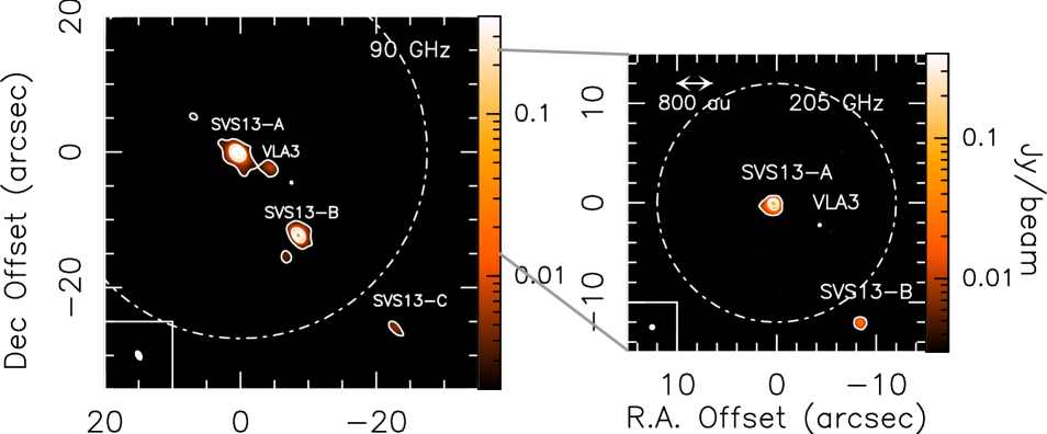
Figure 1: Left Panel: The SVS13-A region as observed in dust continuum emission at 3mm (see Sect. 2) using IRAM NOEMA. Angular offset are with respect to the phase center (see Sect. 3). First contour and steps are, respectively, 5$\sigma$ (1$\sigma$ = 100 $\mu$Jy) and 50$\sigma$. The filled ellipse shows the synthesised beam (HPBW): 1$\aas@@fstack{\prime\prime}$6 $\times$ 1$\aas@@fstack{\prime\prime}$1 (PA= 41^∘). The SVS13-B, SVS13-C, and VLA3 protostars are also labelled. White dashed circle indicate the primary beam: $\sim$ 55$\arcsec$. Right Panel: Zoom-in of the inner SVS13-A region as observed in dust continuum at 1.3mm. First contour and steps are, respectively, 5$\sigma$ (1$\sigma$ = 1 mJy) and 30$\sigma$. Symbols are as in the Left panel. The synthesised beam (HPBW) is 0$\aas@@fstack{\prime\prime}$6 $\times$ 0$\aas@@fstack{\prime\prime}$6 (PA= –46^∘), while the primary beam is 24$\arcsec$.

4.2 Line images and spectra

We imaged, at both 1.4 mm and 3mm, a large (32) number of lines of S-bearing species, listed in Table 1. Namely, 4 ³²SO (hereafter SO) lines ($E_{\rm u}$ in the 9–39 K range), 2 ³⁴SO lines (9–19 K), 7 SO₂ lines (37–549 K), 2 ³⁴SO₂ lines (55–70 K), 1 C³²S (hereafter CS) line (7 K), 1 C³⁴S line (6 K), 1 C³³S line (7 K), 3 OCS lines (16–89 K), 9 H₂C³²S (hereafter H₂CS) lines (including two pairs blended at the present spectral resolution; 10–244 K), 1 H₂C³⁴S line (48 K), and 1 NS line (27 K). In the following, for sake of clarity, the results of each species will be reported separately. The overall picture will be discussed in Sect. 6.

4.2.1 SO

Figure 2-Left shows the spatial distribution of the low-$E_{\rm u}$ (9 K) SO(2₃–1₂) emission observed at 86 GHz. The emission peaks are towards SVS13-A and SVS13-B (3mm continuum drawn in black) and are spatially unresolved. In addition, a contribution from the extended envelope is suggested. Figure 3 reports the SVS13-A spectrum. The used low-spectral resolution (7 km s^-1) prevents us from a proper kinematical analysis. However, the peak velocity is centred at the systemic velocity of +8.6 km s^-1 (Chen et al., 2009). By imaging the SO(2₃–1₂) per velocity range, Fig. 2-Left shows some blue-shifted emission flowing towards South-East, i.e. tracing signatures of the well-known extended ($\gg$ 8$\arcsec$) outflow associated with HH7-11 (see e.g. Lefloch et al. 1998; Codella et al. 1999; Lefèvre et al. 2017). In addition, a well collimated (and more compact) bipolar outflow driven by SVS13-B is observed. Very high-velocity emission, up to +20 km s^-1 and down to –94 km s^-1, is detected. This outflow, located along the NW-SE direction, had been discovered by (Bachiller et al., 1998) using SiO, and recently imaged in the context of the CALYPSO IRAM Large Program Maury et al. (2019) by Podio et al. (2021) in the SiO(5–4), CO(2–1), and SO(5₆-4₅) lines. The outflow collimation is consistent with SVS13-B being in an earliest evolutionary stage (Class 0) with respect to SVS13-A (Class I) driving a more extended, and less collimated flow.

Moving towards slightly higher excitation lines (up to 39 K), the SO lines observed at 3mm with $\sim$ 1$\aas@@fstack{\prime\prime}$5 (450 au) angular resolution appear spatially unresolved and centred on SVS13-A. SVS13-B is detected only through the 2₂–1₁ and 2₃–1₂ lines. On the other hand, the images of the SO lines at 1.4mm (synthesised beam $\sim$ 180 au) reveal a structure with a size $\sim$ 300 au, plausibly associated with the molecular envelope. An elongation (due to low-velocity blue-shifted emission) towards the blue-shifted outflow SE direction is clearly visible. The SO(4₅–3₄) line ($E_{\rm u}$ = 39 K) profile, observed with a spectral resolution of 2.8 km s^-1, has a FWHM line width of 9.2 km s^-1.

Finally, the ratio between the integrated fluxes as derived towards SVS13-A of the SO and ³⁴SO 2₃–1₂ or 2₂–1₁ lines is $\sim$10–12, which, assuming optically thin ³⁴SO emission and ³²S/³⁴S = 22 (Wilson & Rood, 1994), leads to an SO opacity $\sim$ 1.

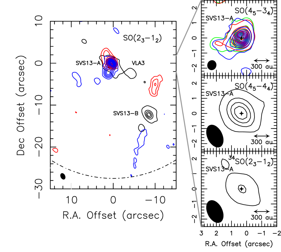
Figure 2: Left Panel: Spatial distribution of the SVS13-A region obtained using the SO(2₃–1₂) red- and blue-shifted emission overlaid with the 90 GHz continuum map (see Fig. 1). Red-shifted emission maps have been derived by integrating the SO emission from the systemic velocity (+8.6 km s^-1, Chen et al. (2009)) up to +20 km s^-1. Blue-shifted image has been obtained by integrating down to –94 km s^-1 in absolute values). Angular offset are with respect to the phase center (see Sect. 3). First contour and steps are, respectively, 3$\sigma$, and 4$\sigma$, respectively. The 1$\sigma$ value is 5 mJy km s^-1 and 14 mJy km s^-1 for the red- and blue-shifted emission, respectively. The filled ellipse shows the synthesised beam (HPBW): 1$\aas@@fstack{\prime\prime}$6 $\times$ 1$\aas@@fstack{\prime\prime}$1 (PA= 41^∘). The SVS13-B protostar is also labelled. White dashed circle indicate the primary beam: $\sim$ 55$\arcsec$. Upper-Right Panel: Zoom-in of the inner SVS13-A region as observed using the SO(4₅–3₄) emission. Green contours are for the emission in the 3 km s^-1 around the systemic velocity. Red-shifted emission maps has been derived by integrating the SO emission from the systemic velocity up to +20 km s^-1. Blue-shifted image has been obtained by integrating down to –5 km s^-1. First contour and steps are, respectively, 3$\sigma$, and 10$\sigma$. The 1$\sigma$ value is 10 mJy km s^-1 (systemic velocity), 13 mJy km s^-1 (red), and 11 mJy km s^-1 (blue). Symbols are as in the Left panel. The black cross indicates the positions of the 205 GHz continuum peak (see Fig. 1). The synthesised beam (HPBW) is 0$\aas@@fstack{\prime\prime}$65 $\times$ 0$\aas@@fstack{\prime\prime}$58 (PA= –46^∘). Middle-Right Panel: Zoom-in of the inner SVS13-A region as observed using the SO(4₅–4₄) emission. The whole velocity emitting region has been used (see Fig. 3). First contour and steps are, respectively, 3$\sigma$ (9 mJy km s^-1), and 10$\sigma$. Symbols are as in the Left panel. The synthesised beam (HPBW) is: 1$\aas@@fstack{\prime\prime}$6 $\times$ 1$\aas@@fstack{\prime\prime}$1 (PA= 41^∘). Bottom-Right Panel: Zoom-in of the inner SVS13-A region as observed using the ³⁴SO(2₃–1₂) emission. First contour and steps are, respectively, 3$\sigma$ (12 mJy km s^-1), and 10$\sigma$. Symbols are as in the Left panel. The synthesised beam is as in the Middle-Right panel.

Figure 3: Observed SO, and ³⁴SO spectra (in T_B scale, see Table 1) extracted at the emission peak: $\alpha_{2000}$ = 03^h29^m03^s.75, $\delta_{2000}$ = +31^∘16^′03^′′.8. Transitions and corresponding upper level energies are reported. The vertical dashed line stands for the ambient LSR velocity (+8.6 km s^-1, Chen et al. (2009)). Note that the p-H₂CS(6_2,4–5_2,3) appears close to the SO(4₅–3₄) profile (see Tab. 1).

4.2.2 CS

We imaged the $J$ = 2–1 line emission of the CS, C³⁴S, and C³³S isotoplogues, emitting in the 96.4–98.0 GHz spectral range (Table 1). Figure 4 shows how the main isotopologue is tracing the molecular envelope around SVS13-A. The rarer isotopologues are emitting towards the CS emission peak, having a spatially unresolved structure ($\leq$ 450 au). The spectra corresponding to the CS peak are drawn in Fig. 5. The line ratios observed towards SVS13-A are: CS/C³⁴S $\simeq$ 3 and CS/C³³S $\simeq$ 11. In turn, assuming the C³³S emission to be optically thin and ³²S/³³S = 138 (Wilson & Rood, 1994), this implies optically thick ($\tau$ $\sim$ 14) CS emission. The C³⁴S emission results to be moderately thick ($\tau_{\rm C^{34}S}$ $\simeq$ 2).

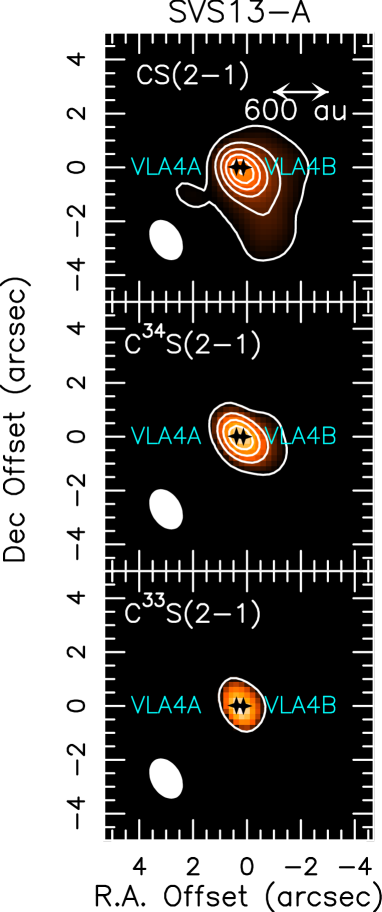
Figure 4: Spatial distribution of the SVS13-A region obtained using the $J$ = 2–1 CS (Upper panel), C³⁴S (Middle), and C³³S (Bottom) line emission (contours and colour). The whole velocity emitting region has been used (down to – 5 km s^-1 and up to +25 km s^-1, depending on the line, see Fig. 5). Angular offset are respect to the phase center (see Sect. 3). First contour and steps are, respectively, 5$\sigma$, and 10$\sigma$, respectively. The 1$\sigma$ value is 10 mJy km s^-1 (CS), and 4 mJy km s^-1 (C³⁴S, C³³S). The filled ellipse shows the synthesised beam (HPBW): 1$\aas@@fstack{\prime\prime}$6 $\times$ 1$\aas@@fstack{\prime\prime}$1 (PA= 41^∘). The black crosses indicate the positions of the VLA4A and VLA4B sources as imaged using the VLA array by Tobin et al. (2018).

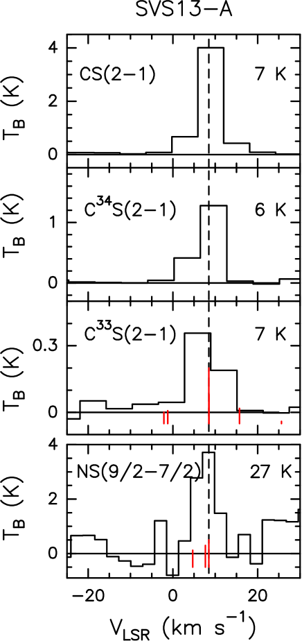
Figure 5: Observed CS, C³⁴S, C³³S, and NS spectra (in T_B scale, see Table 1) extracted at the emission peak: $\alpha_{2000}$ = 03^h29^m03^s.75, $\delta_{2000}$ = +31^∘16^′03^′′.8. Transitions and corresponding upper level energies are reported. The vertical dashed line stands for the ambient LSR velocity (+8.6 km s^-1, Chen et al. (2009)). The C³³S(2–1) line consists of 6 hyperfine components with $S\mu^{2}$ in the 0.5–12.2 D² range (Bogey et al., 1981; Lovas, 2004; Müller et al., 2005) spread on a 9 MHz frequency interval. The vertical red lines (in scales according to their $S\mu^{2}$) indicated their relative offset in velocity scale with respect to the brightest $F$=5/2–3/2 line. The NS 9/2–7/2 $\Omega$=1/2 line consists of 3 hyperfine components (Lee et al., 1995) associated with $S\mu^{2}$ in the 10.9–17.4 D² range spread on a 0.6 MHz frequency interval. The vertical red lines (in scales according to their $S\mu^{2}$) indicated their relative offset in velocity scale with respect to the brightest $F$=11/2–9/2 line (see Table 1).

4.2.3 SO₂

A large number of SO₂ (and ³⁴SO₂) lines has been detected at both 3mm and 1.4mm, covering a very large range of the upper level energies, from 37 K to 549 K. Figure 6 reports a selection of the spatial distributions of the SO₂ lines, peaking towards SVS13-A. All the spectra are reported in Fig. 7: when observed with a spectral resolution of 2.9 km s^-1, the profiles peak close to the systemic velocity (+8.6 km s^-1, Chen et al. 2009), and are $\sim$ 7–8 km s^-1 broad.

Contrarily to SO and CS, the SO₂ emission is spatially unresolved both at 3mm and 1.4mm, indicating an emitting size less than 180 au. In other words, there is neither signature of outflows (as for SO) nor of the envelope revealed by SO and CS. The SO₂ and ³⁴SO₂ emission is tracing the inner protostellar region. By fitting the position of the brightest SO₂ line (204.2 GHz) using a Gaussian fit in the $uv$ domain, we found $\alpha_{2000}$ = 03^h29^m03^s.755, $\delta_{2000}$ = +31^∘16^′03^′′.782. The $uv$ fit error is 3 mas. This position lies between the coordinates of the binary components VLA4A and VLA4B (see Fig. 6-Right panels), more specifically at $\simeq$ 0$\aas@@fstack{\prime\prime}$13 (39 au) from both protostars. This shift perfectly agrees with what was found using iCOMs emission as imaged with an angular resolution of 0$\aas@@fstack{\prime\prime}$4–1$\aas@@fstack{\prime\prime}$3 (at 1.3–3mm) in the context of the CALYPSO project (De Simone et al., 2017; Belloche et al., 2020).

Finally, since we have not detected common SO₂ and ³⁴SO₂ lines, the estimate on the SO₂ opacity will be discussed in Sect. 5 in light of the Large Velocity Gradient (LVG) analysis.

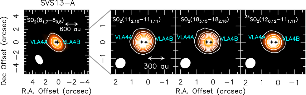
Figure 6: Spatial distribution (contours and colour) of the SVS13-A region obtained using different SO₂, and ³⁴SO₂ line emission (see Table 1). Angular offset are respect to the phase center (see Sect. 3). The whole velocity emitting region has been used (from 0 km s^-1 to +20 km s^-1, see Fig. 7). The SO₂(11_2,10–11_1,11) profile has been deblended by the CH₃OCHO line fitting the profile with two Gaussians (see Table 1). First contour and steps are, respectively, 5$\sigma$, and 10$\sigma$, respectively. The 1$\sigma$ value is: 7 mJy km s^-1 for SO₂(8_1,7–8_0,8 (Left panel), 14 mJy km s^-1 for SO₂(11_2,10–11_1,11), SO₂(18_3,15–18_2,16), and ³⁴SO₂(12_0,12–11_1,11). The filled ellipse shows the synthesised beam (HPBW): 1$\aas@@fstack{\prime\prime}$6 $\times$ 1$\aas@@fstack{\prime\prime}$1 (PA= 41^∘) for the SO₂(8_1,7–8_0,8) maps (Left panel), and 0$\aas@@fstack{\prime\prime}$65 $\times$ 0$\aas@@fstack{\prime\prime}$58 (PA= –46^∘) for the the other images. The black crosses indicate the positions of the VLA4A and VLA4B sources as imaged using the VLA array by Tobin et al. (2018).

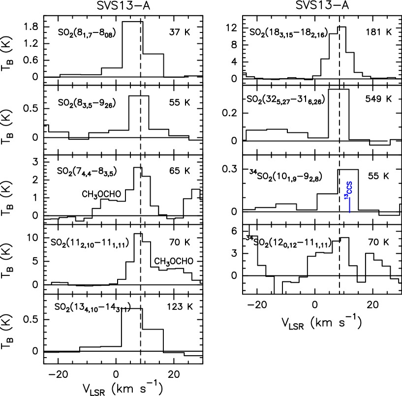
Figure 7: Observed SO₂, ³⁴SO₂, and ³³SO₂ spectra (in T_B scale, see Table 1) extracted at the emission peak: $\alpha_{2000}$ = 03^h29^m03^s.75, $\delta_{2000}$ = +31^∘16^′03^′′.8. Transitions and corresponding upper level energies are reported. The vertical dashed line stands for the ambient LSR velocity (+8.6 km s^-1, Chen et al. (2009)). The ³⁴SO₂ line at $E_{\rm u}$ = 55 K could be contaminated by ¹³CCS emission with $E_{\rm u}$ = 22 K (see Table 1).

4.2.4 OCS

Figure 8 shows the spatial distribution of the three detected OCS lines. The $J$ = 7–6 and 8–7 transitions fall in the 3mm band: the emitting size is clearly unresolved with the spatial resolution of 1$\aas@@fstack{\prime\prime}$5. Also the OCS(17–16) line, imaged with a synthesised beam of 0$\aas@@fstack{\prime\prime}$6, is spatially unresolved. The $uv$ analysis leads to a peak coordinates of $\alpha_{2000}$ = 03^h29^m03^s.754, $\delta_{2000}$ = +31^∘16^′03^′′.778, with an error of 5 mas. This position is consistent with what found using SO₂, lying between the VLA4A and VLA4B positions. The OCS spectra are reported in Fig. 9: the peak velocity is in agreement with the SVS13-A systemic velocity of +8.6 km s^-1 (Chen et al., 2009). In addition the OCS(17–16) profile, samples with a 2.8 km s^-1, shows a FWHM of 7 km s^-1, consistent with those of the SO₂ lines observed at the same angular resolution.

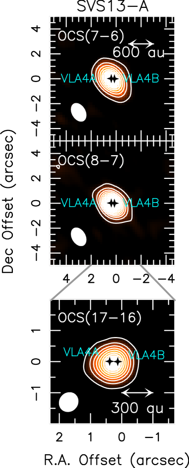
Figure 8: Spatial distribution of the SVS13-A region obtained using the OCS(7–6) (Upper panel), OCS(8–7) (Middle), and OCS(17–16) (Bottom) line emission (contours and colour). The whole velocity emitting region has been used (from 0 km s^-1 to +20 km s^-1, see Fig. 9). Angular offset are with respect to the phase center (see Sect. 3). First contour and steps are, respectively, 5$\sigma$, and 10$\sigma$, respectively. The 1$\sigma$ value is 5 mJy km s^-1 ($J$ = 7–6, and 8–7), and 26 mJy km s^-1 ($J$ = 17–16). The filled ellipse shows the synthesised beam (HPBW): 1$\aas@@fstack{\prime\prime}$6 $\times$ 1$\aas@@fstack{\prime\prime}$1 (PA= 41^∘) for OCS(7–6) and OCS(8–7), and and 0$\aas@@fstack{\prime\prime}$65 $\times$ 0$\aas@@fstack{\prime\prime}$58 (PA= –46^∘) for OCS(17–16). The black crosses indicate the positions of the VLA4A and VLA4B sources as imaged using the VLA array by Tobin et al. (2018).

Figure 9: Observed OCS spectra (in T_B scale, see Table 1) extracted at the emission peak: $\alpha_{2000}$ = 03^h29^m03^s.75, $\delta_{2000}$ = +31^∘16^′03^′′.8. Transitions and corresponding upper level energies are reported. The vertical dashed line stands for the ambient LSR velocity (+8.6 km s^-1, Chen et al. (2009)).

4.2.5 H₂CS

As reported in Table 1, ten H₂CS and H₂CS³⁴S lines, with $E_{\rm u}$ in the 10–244 K range, have been revealed using both setups at 3mm and 1.4mm. Two pairs of SO₂ lines are blended at the present spectral resolution. Figure 10 shows examples of the spatial distributions of the H₂CS lines: as SO₂ and OCS, the emission is peaking towards SVS13-A, being spatially unresolved at both 3mm and 1.4mm.

The peak coordinates, according to the $uv$ fit, are $\alpha_{2000}$ = 03^h29^m03^s.752, $\delta_{2000}$ = +31^∘16^′03^′′.786, with an error of 8 mas, in agreement with the SO₂ and OCS ones. The profiles at the peak emission are shown in Fig. 11. Interestingly, o-H₂C³⁴S(6_1,5–5_1,4) has been observed with a spectral resolution of 0.9 km s^-1, i.e. definitely better than that of the other lines (3–7 km s^-1). For this line the profile is well sampled, peaking at the SVS13-A systemic velocity (+8.6 km s^-1, Chen et al. 2009), and with a FWHM of 2.7 km s^-1.

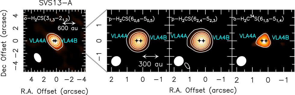
Figure 10: Spatial distribution (contours and colour) of the SVS13-A region obtained using different H₂CS, and H₂C³⁴S line emission (see Table 1). The whole velocity emitting region has been used (from 0 km s^-1 to +20 km s^-1, see Fig. 11). The p-H₂CS(6_2,4–5_2,3) emission has been deblended from the SO emission (see Table 1) applying two Gaussian profiles. Angular offset are relative to the phase center (see Sect. 2). First contour and steps are, respectively, 5$\sigma$, and 10$\sigma$, respectively. The 1$\sigma$ value, from Left to Right, is 5, 13, 11, and 9 mJy km s^-1, respectively. The filled ellipse shows the synthesised beam (HPBW): 1$\aas@@fstack{\prime\prime}$6 $\times$ 1$\aas@@fstack{\prime\prime}$1 (PA= 41^∘) for the o-H₂CS(3_1,3–2_1,2) line (Left panel), and 0$\aas@@fstack{\prime\prime}$65 $\times$ 0$\aas@@fstack{\prime\prime}$58 (PA= –46^∘) for the p-H₂CS(6_0,6–5_0,5), p-H₂CS(6_2,4–5_2,3), and o-H₂C³⁴S(6_1,5–5_1,4) lines (Middle and Right panels). The black crosses indicate the positions of the VLA4A and VLA4B sources as imaged using the VLA array by Tobin et al. (2018).

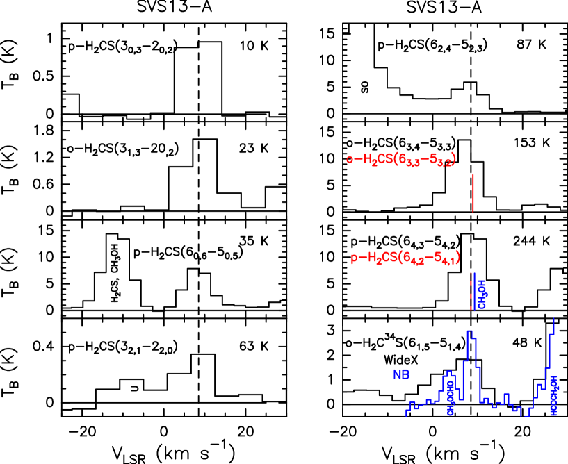
Figure 11: Observed H₂CS, and H₂C³⁴S spectra (in T_B scale, see Table 1) extracted at the emission peak: $\alpha_{2000}$ = 03^h29^m03^s.75, $\delta_{2000}$ = +31^∘16^′03^′′.8. Transitions and corresponding upper level energies are reported. The vertical dashed line stands for the ambient LSR velocity (+8.6 km s^-1, Chen et al. (2009)). Red labels and red vertical segments denote two H₂CS profiles with the same $E_{\rm u}$ value and blended at the present spectral resolution (Table 1). The black vertical labels indicate that the line is reported in another panel of the present figure. The H₂CS doublets at $E_{\rm u}$ = 244 K could be contaminated by CH₃OH emission with $E_{\rm u}$ = 317 K (see Table 1). The H₂C³⁴S(6_1,5–5_1,4) profile has been observed using both low- (black histogram) and high-spectral (blue) backends (see Sect. 2: labelled Widex and NB, respectively).

4.2.6 NS

The NS(9/2–7/2) $\Omega$=1/2 line, with $E_{\rm u}$ = 27 K, has been detected towards SVS13-A. The profile consists of three hyperfine components, blended with the 2.8 km s^-1 spectral resolution (see Fig. 5). The frequency transitions is 207.4 GHz and the corresponding spatial distribution is shown in Fig. 12. The emitting size is unresolved, being less than the 0$\aas@@fstack{\prime\prime}$6 synthesised beam. The emission peaks between the positions of the VLA4A and VLA4B, namely at $\alpha_{2000}$ = 03^h29^m03^s.750, $\delta_{2000}$ = +31^∘16^′03^′′.808, with an error of 14 mas. In summary, NS, OCS, SO₂, H₂CS, once observed with the present spatial resolution ($\sim$ 100 au) are tracing the same spatially unresolved region, being consistent with what expected from a chemical enriched region around the protostar(s), i.e. the hot corino(s). These findings will be discussed in Sect. 6 in light of the physical parameters derived in Sect. 5.

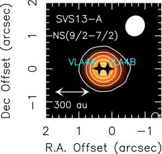
Figure 12: Spatial distribution (contours and colour) of the SVS13-A region obtained using the NS(9/2–7/2) $\Omega$=1/2 emission. The whole velocity emitting region has been used (from 0 km s^-1 to +15 km s^-1. The line profile consists of three hyperfine components, blended at the present spectral resolution (see Fig. 5 and Table 1). Angular offset are relative to the phase center (see Sect. 3). First contour and steps are, respectively, 5$\sigma$ (50 mJy km s^-1), and 10$\sigma$, respectively. The filled ellipse shows the synthesised beam (HPBW): 0$\aas@@fstack{\prime\prime}$65 $\times$ 0$\aas@@fstack{\prime\prime}$58 (PA= –46^∘). The black crosses indicate the positions of the VLA4A and VLA4B sources as imaged using the VLA array by Tobin et al. (2018).

Table 1: List of transitions of S-bearing species detected towards SVS13-A. The Gaussian fit parameters (in $T_{\rm MB}$ scale) refer to the spectra extracted at the emission peak: $\alpha_{2000}$ = 03^h29^m03^s.75, $\delta_{2000}$ = +31^∘16^′03^′′.8.

Transition	$\nu$a	$E_{\rm up}$a	$S\mu^{2}$a	$d$v	rms	$T_{\rm peak}$	$V_{\rm peak}$	FWHM	$I_{\rm int}$
	(MHz)	(K)	(D2)	(km s-1)	(mK)	(mK)	(km s-1)	(km s-1)	(K km s-1)
SO
22–11	86093.95	19	3.5	7.0	22	2765(98)	+8.9(0.2)	9.7(0.5)	27.69(0.23)
23–12	99299.87	9	6.9	6.0	42	4191(42)	+8.7(0.2)	9.4(0.7)	44.30(1.99)
45–44	100029.64	39	0.8	6.0	23	1209(43)	+8.8(0.2)	7.5(0.5)	9.55(0.27)
45–34	206176.01	39	8.9	2.8	920	43142(777)	+8.3(0.2)	9.2(0.2)	422.00(7.38)
34SO
22–11	84410.69	19	3.5	7.1	54	296(12)	+9.2(4.2)	7.2(5.1)	2.29(0.68)
23–12	97715.32	9	6.9	6.1	120	436(4)	+8.2(1.1)	9.7(7.0)	4.48(1.20)
SO2
134,10–143,11	82951.94	123	5.1	7.1	57	751(23)	+7.6(1.7)	9.9(1.5)	7.96(0.68)
81,7–80,8	83688.09	37	17.0	7.2	72	2071(24)	+7.0(0.3)	10.3(0.5)	22.65(0.94)
325,27–316,26	84320.88	549	13.5	7.1	40	364(30)	+8.0(2.3)	7.1(6.1)	2.76(0.65)
83,5–92,6	86639.09	55	3.0	6.9	53	719(22)	+8.1(1.3)	8.9(1.4)	6.82(0.73)
183,15–182,16	204246.76	181	34.5	2.9	780	12609(160)	+8.2(0.2)	7.6(0.5)	102.64(5.5)
74,4–83,5	204384.30	65	1.7	2.9	540	2757(210)	+8.0(0.7)	7.9(1.6)	23.09(4.12)
112,10–111,11	205300.57	70	12.1	2.9	197	11235(230)	+8.7(0.8)	7.3(1.9)	87.28(19.24)
34SO2
101,9–92,8b	82124.35	55	6.5	7.1	160	6998(55)	+9.4(1.2)	8.3(3.2)	63.29(3.03)
120,12–111,11	204136.23	70	22.7	2.9	1400	5982(780)	+9.1(0.7)	5.4(2.0)	34.56 (9.4)
CS
2–1	97980.95	7	7.6	6.1	38	5196(12)	+8.6(0.2)	7.0(0.3)	38.72(0.62)
C34S
2–1	96412.95	6	7.6	6.2	45	2088(27)	+7.8(1.4)	6.4(4.8)	14.26(4.38)
C33S
2–1 $F$=5/2–3/2c	97171.84	7	12.2	6.2	29	388(32)	+8.2(0.5)	8.6(1.2)	3.56(0.33)
OCS
7–6	85139.10	16	3.5	7.0	36	3787(50)	+8.5(0.4)	7.1(0.2)	28.39(0.34)
8–7	97301.21	21	4.1	6.1	29	5031(86)	+8.6(0.2)	7.6(0.2)	40.73(1.18)
17–16	206745.16	89	8.7	2.8	471	40764(140)	+8.4(0.3)	7.1(0.7)	308.66(4.89)
H2CS
o-31,3–21,2	101477.81	23	21.8	5.9	20	1576(12)	+8.6(1.4)	10.0(3.3)	17.12(4.50)
p-30,3–20,2	103040.45	10	8.2	5.8	33	1603(93)	+8.5(1.3)	6.2(3.3)	10.49(2.26)
p-32,1–22,0	103051.87	63	4.5	5.8	46	318(18)	+7.8(4.7)	9.9(4.5)	3.79(1.15)
p–60,6–50,5	205987.86	35	16.3	2.8	159	7702(79)	+8.2(0.2)	7.0(0.2)	57.35(0.56)
p-64,3–54,2d	206001.88d	244	9.0
				} 2.8	115	15074(260)	+8.8(0.2)	7.3(0.2)	116.65(1.84)
p-64,2–54,1d	206001.88d	244	9.0
o-63,4–53,3d	206051.94d	153	36.6
				} 2.8	161	13512(120)	+7.1(0.8)	7.6(2.1)	108.84(24.75)
o-63,3–53,2d	206052.24d	153	36.6
p-62,4–52,3e	206158.60e	87	14.5	2.8	160	6004(120)	+7.9(0.2)	7.7(0.5)	48.87(0.49)
H2C34S
o-61,5–51,4	205583.13	48	47.5	0.9	560	3113(190)	+8.6(0.2)	2.7(0.5)	8.91(1.36)
NS
9/2–7/2 $\Omega$=1/2f l=e	207436.05	27	17.4	2.8	1100	3968(840)	+7.9(0.8)	5.7(1.7)	24.22(6.41)
NS+
2–1	100198.55	7	8.7	6.0	28	–	–	–	$\leq$ 1g

^a Spectral parameters from the Cologne Database for Molecular Spectroscopy (Müller et al., 2001, 2005) for all the species, with the exception of those of the H₂CS isotoplogues, derived from the Jet Propulsion Laboratory (JPL Pickett et al., 1998), and those of NS⁺, from Cernicharo et al. (2018). ^b Possible contamination with ¹³CCS emission at 82123.376 MHz ($E_{\rm u}$ = 22 K, $S\mu^{2}$ = 0.7 D²). ^c The C³³S(2–1) line consists of 6 hyperfine components (Bogey et al., 1981; Lovas, 2004; Müller et al., 2005) in a 9 MHz frequency interval. The line with the highest $S\mu^{2}$ is reported (see Fig. 5). ^d Lines blended at the present spectral resolution (2 MHz). Possible contamination with CH₃OH emission at 206001.30 MHz ($E_{\rm u}$ = 317 K, $S\mu^{2}$ = 10.2 D²). ^e Contaminated by SO(4₅–3₄) high-velocity emission. ^f The 9/2–7/2 $\Omega$=1/2 line consists of 3 hyperfine components (Lee et al., 1995) in a 0.6 MHz frequency interval. The line with the highest $S\mu^{2}$ $F$=11/2–9/2 is reported (see Fig. 5). ^g 3$\sigma$ upper limit.

5 Physical parameters

We analysed the SO, SO₂ and H₂CS (and their isotopologues) spectra extracted at the emission peak ($\alpha_{2000}$ = 03^h29^m03^s.75, $\delta_{2000}$ = +31^∘16^′03^′′.8) via the non-LTE (Local Thermodynamic Equilibrium) Large Velocity Gradient (LVG) approach using the code grelvg described in Ceccarelli et al. (2003). We assumed a Boltzmann distribution for the H₂ ortho-to-para ratio. For SO, we used the collisional coefficients with p-H₂ computed by Lique et al. (2007) and retrieved from the BASECOL database (Dubernet et al., 2013). For SO₂, we used the collisional coefficients with ortho- and para-H₂ computed by Balança et al. (2016) and retrieved from the LAMDA database (Schöier et al., 2005). For H₂CS, we used the H₂CO-H₂ collisional coefficients with ortho- and para-H₂ derived by Wiesenfeld & Faure (2013), scaled them for the mass ratio, and provided by the LAMDA database (Schöier et al., 2005).

We assumed a semi-infinite slab geometry to compute the line escape probability (Scoville & Solomon, 1974) and assumed a line width equal to 8 km s^-1. We used the ³²S/³⁴S equal to 22 (Wilson & Rood, 1994), and an H₂CS ortho-to-para ratio equal to 3. Finally, the errors on the observed line intensities have been obtained adding the spectral r.m.s. to the uncertainties due to calibration (see Sect. 3). We ran large grids of models varying the kinetic temperature ($T_{\rm kin}$) from 20 to 500 K, the volume density ($n_{\rm H_{2}}$) from 10⁴ cm^-3 to 10⁹ cm^-3, the emitting sizes from 0$\aas@@fstack{\prime\prime}$1 to 30$\arcsec$ and the SO, SO₂ and H₂CS column densities from 10¹⁵ cm^-2 to 10²¹ cm^-2. The best fit for each species is obtained by simultaneously minimizing the difference between the predicted and observed integrated intensities of both used isotopologues (e.g. SO and ³⁴SO; SO₂ and ³⁴SO₂; H₂CS and H₂C³⁴S).

The results obtained for SO show a best solution, characterised by $\chi^{2}$ $\simeq$ 2, with a total column density N_SO of 10¹⁷ cm^-2, a kinetic temperature $T_{\rm kin}$ equal to 280 K, and the volume density $n_{\rm H_{2}}$ being 10⁸ cm^-3. The size is 0$\aas@@fstack{\prime\prime}$3 (90 au). The line opacities lies between 0.1 and 1.4. If we consider an uncertainty of 1 $\sigma$, which correspond to a probability of 30% to exceeding $\chi^{2}$, we have $T_{\rm kin}$ $\geq$ 150 K, $n_{\rm H_{2}}$ $\geq$ 6 $\times$ 10⁶ cm^-3, N_SO = 0.2–3 $\times$ 10¹⁷ cm^-2, and sizes in the 0$\aas@@fstack{\prime\prime}$2–0$\aas@@fstack{\prime\prime}$5 range.

The analysis of SO₂ leads to a best solution ($\chi^{2}$ $\simeq$ 3) with the N${}_{\rm SO_{2}}$ = 10¹⁸ cm^-2, $T_{\rm kin}$ = 210 K, and 10⁸ cm^-3. The size is 0$\aas@@fstack{\prime\prime}$2 ($\sim$ 60 au). The line emission is moderately thick, being the opacity between 0.30 and 4.5. Once considered the uncertainty of 1 $\sigma$, we obtain $T_{\rm kin}$ $\simeq$ 100–300 K, and $n_{\rm H_{2}}$ $\geq$ 5 $\times$ 10⁶ cm^-3, N${}_{\rm SO_{2}}$ = 0.3–3 $\times$ 10¹⁸ cm^-2, and the size between 0$\aas@@fstack{\prime\prime}$1 and 0$\aas@@fstack{\prime\prime}$3.

The best fit obtained for H₂CS, identified by $\chi^{2}$ $\simeq$ 0.1, indicates the total column density equal to 2 $\times$ 10¹⁵ cm^-2, a size of 0$\aas@@fstack{\prime\prime}$4 (120 au), the kinetic temperature $T_{\rm kin}$ = 100 K, and the volume density $n_{\rm H_{2}}$ = $2\times$ 10⁵ cm^-3. The line opacities are all in the 0.04–0.4 range but that of the 6_0,6–5_0,5 para line which is 0.86. Taking into account 1 $\sigma$, the following constraints are derived: $T_{\rm kin}$ $\geq$ 50 K, $n_{\rm H_{2}}$ $\geq$ 10⁵ cm^-3, N${}_{\rm H_{2}CS}$ = 0.7–2 $\times$ 10¹⁵ cm^-2, and sizes in the 0$\aas@@fstack{\prime\prime}$2–0$\aas@@fstack{\prime\prime}$8 range.

Figure 13 shows the comparison between observations and best-fit line predictions for SO, SO₂, and H₂CS, while Table 2 summarises the excitation ranges found for the three molecules. As a matter of fact, all the SO, SO₂ and H₂CS analysis are consistent with the occurrence of hot corino emission. This will allow us to compare the present results with what previously found using iCOMs (see Sect. 6).

Table 2: 1$\sigma$ Confidence Level (range) from the Non-LTE LVG Analysis of the SO, SO₂, and H₂CS lines towards SVS13-A as imaged with NOEMA. The OCS, CS, and NS column densities, derived assuming LTE conditions, are also reported. The last row with H₂S, is based on IRAM 30-m data at 1.4mm. The last column is for the abundance with respect to H₂.

Species	Ntot	n${}_{\rm H_{2}}$	Tkin	size	X${}_{\rm H_{2}}$d
	(cm-2)	(cm-3)	(K)	(arcsec)
SO	0.2-3 $\times$ 1017	$\geq$ 6 $\times$ 106	$\geq$ 150 K	0$\aas@@fstack{\prime\prime}$2–0$\aas@@fstack{\prime\prime}$5	7 $\times$ 10-9 – 1 $\times$ 10-7
SO2	0.3-3 $\times$ 1018	$\geq$ 5 $\times$ 106	100–300	0$\aas@@fstack{\prime\prime}$1–0$\aas@@fstack{\prime\prime}$3	1–10 $\times$ 10-7
H2CS	0.7-2 $\times$ 1015	$\geq$ 105	$\geq$ 50 K	0$\aas@@fstack{\prime\prime}$2–0$\aas@@fstack{\prime\prime}$8	2–7 $\times$ 10-10
	Ntot	n${}_{\rm H_{2}}$	Trot	size	X${}_{\rm H_{2}}$d
	(cm-2)	(cm-3)	(K)	(arcsec)
OCSa	1-2 $\times$ 1015	–	70–170	0$\aas@@fstack{\prime\prime}$3a	3–7 $\times$ 10-10
CSb	0.8-17 $\times$ 1018	–	37.5c–300	0$\aas@@fstack{\prime\prime}$3b	0.3–6 $\times$ 10-6
NSb	1-6 $\times$ 1015	–	37.5c–300	0$\aas@@fstack{\prime\prime}$3b	0.2–3 $\times$ 10-9
NS+b	$\leq$ 8 $\times$ 1014	–	37.5c–300	0$\aas@@fstack{\prime\prime}$3b	$\leq$ 3 $\times$ 10-10
H2Sb,e	0.5–1 $\times$ 1018	–	37.5c–300	0$\aas@@fstack{\prime\prime}$3b	2–4 $\times$ 10-7

^a Estimate derived using the RD approach, and assuming a source size of 0$\aas@@fstack{\prime\prime}$3 following the SO, SO₂, and H₂CS LVG analysis. ^b Estimates derived using one line, and assuming: (i) a source size of 0$\aas@@fstack{\prime\prime}$3, and a temperature in the 37.5–300 K range (from LVG analysis of SO, SO₂, and H₂CS). For CS, we took into account the line opacity of 14 derived from the comparison with the emission of C³⁴S and C³³S. ^c For T_rot we conservatively used a lower limit of 37.5 K, according to the partition function tabulated in the Jet Propulsion Laboratory (JPL, Pickett et al., 1998) database. ^d We assume N${}_{\rm H_{2}}$= 3 $\times$ 10²⁴ cm^-2 (Chen et al., 2009). ^e Estimated based on the 2_2,0–2_1,1 line observed with a HPBW = 11$\arcsec$ using the IRAM 30-m antenna (see Sect. 6.4).

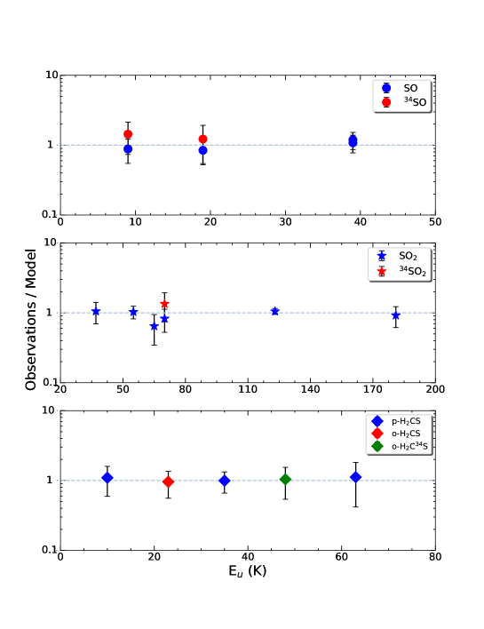
Figure 13: Ratio of the observed and best-fit theoretical line integrated intensities of SO (Upper panel), SO₂ (Middle), and H₂CS (Bottom) as a function of the line upper-level energy (see the text and Table 2). Different symbols indicate different isotopologues as well as ortho and para species.

For OCS, having detected three lines, two of them at very similar upper level excitation (16 K and 21 K), we did not apply the LVG analysis, adopting instead the rotational diagram (RD) approach, where LTE population and optically thin lines are assumed. Under these assumptions, for a given molecule, the relative population distribution of all the energy levels, is described by a Boltzmann temperature, that is the rotational temperature $T_{\rm rot}$. Given the OCS emission is peaking towards SVS13-A and spatially unresolved (Fig. 8), we corrected the line intensities assuming a size of 0$\aas@@fstack{\prime\prime}$3, i.e. the average size obtained from the LVG results for SO, SO₂, and H₂CS. The RD analysis which provides a column density of 1–2 $\times 10^{15}$ cm^-2, and a rotational temperature T_rot = 120$\pm$50 K (see Fig. 14).

Finally, for CS and NS, having detected only one transition, in light of the previous LVG results we adopted again a source size of 0$\aas@@fstack{\prime\prime}$3 and conservatively assumed the overall temperature range (37.5–300 K, see Table 2). We consequently derived: 0.8–17 $\times 10^{18}$ cm^-2 for CS, and 1–6 $\times 10^{15}$ cm^-2 for NS.

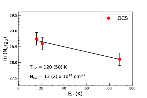
Figure 14: Rotational diagrams for OCS derived using the emission lines observed towards SVS13-A (see Table 1 and Fig. 9). The parameters N_u, g_u, and $E_{\rm up}$ are, respectively, the column density, the degeneracy and the energy (with respect to the ground state of each symmetry) of the upper level. A source size of 0$\aas@@fstack{\prime\prime}$3 has been assumed, following the SO, SO₂, and H₂CS LVG analysis. The derived values of the rotational temperature are reported in the panels.

6 Discussion

6.1 The chemical census of the SVS13-A hot corino

The SVS13-A system has been recently subject of IRAM 30-m (ASAI: Lefloch et al., 2018) and IRAM PdBI (CALYPSO: Maury et al., 2019) observations aimed to obtain its chemical census. More specifically, Bianchi et al. (2017, 2019a) reported the analysis of a large sample of iCOMs using the ASAI single dish unbiased spectral survey: the large number of lines allowed the authors to: (i) analyse using the LVG approach the methanol isotopologues, and (ii) consequently derive the column densities of more complex organic species (CH₃CHO, H₂CCO, HCOOCH₃, CH₃OCH₃, CH₃CH₂OH, NH₂CHO). On the other hand, De Simone et al. (2017) and Belloche et al. (2020) used the PdBI images (synthesised beams between 0$\aas@@fstack{\prime\prime}$5 and 1$\aas@@fstack{\prime\prime}$7) of iCOMs emitting in selected spectral windows to derive the column densities in LTE conditions of, again, a large number of iCOMs, namely those reported by Bianchi et al. (2019a) plus C₂H₅CN, a-(CH₂OH)₂, and HCOCH₂OH. Both the ASAI and the CALYPSO analysis led to an emitting size, for iCOMs, of 0$\aas@@fstack{\prime\prime}$3, perfectly consistent with what is found in the present analysis of S-bearing species (see Table 2). The column densities are also well in agreement, being different by less than a factor of 2 for all the iCOMs in common except for methanol and formamide (a factor of 3–4). Very recently, also Yang et al. (2021) reported the results of the PEACHES ALMA survey on the chemical content of star forming regions in Perseus, SVS13-A among them. A large number of iCOMs are detected, in agreement with the ASAI and CALYPSO results. Column densities, measured in this case of a 0$\aas@@fstack{\prime\prime}$5 source size, are also consistent considering the uncertainties. In conclusion, once observed with a $\sim$ 1$\arcsec$ resolution, it looks that S-bearing species are emitting from a region similar to that associated with the hot corino chemistry.

In order to derive the abundances of S-bearing species we assumed N${}_{\rm H_{2}}$ = 3 $\times$ 10²⁴ cm^-2 as the typical value for the inner 0$\aas@@fstack{\prime\prime}$3 region, following what was adopted by Bianchi et al. (2019a) and Belloche et al. (2020) for the iCOMs analysis, using the continuum images by Chen et al. (2009). The abundances are reported in Table 2: the most abundant S-species are CS (0.3–6 $\times$ 10^-6), SO (7 $\times$ 10^-9 – 1 $\times$ 10^-7), and SO₂ (1–10 $\times$ 10^-7). On the other hand, H₂CS and OCS have similar, lower, abundances (a few 10^-10), while X_NS $\sim$ 10^-10–10^-9. Interestingly, the H₂CS abundance in SVS13-A is four orders of magnitude higher with respect to the recently measured in the H₂CS ring in the protoplanetary disk around the Class II HL Tau (Codella et al., 2020). This strongly supports that sulfur chemistry is indeed definitely evolving during the star-forming process.

Finally, Figure 15 summarises the abundances derived here for the sulfuretted molecules as well as (i) those of iCOMs reported by Bianchi et al. (2019a), (ii) and those derived using the CALYPSO datatset De Simone et al. (2017); Belloche et al. (2020) applying the same H₂ column density. For completeness, we also added 5-atoms molecules such as H₂CCO (Bianchi et al., 2019a), and CH₃CN, and NH₂CN (Belloche et al., 2020). The present census of the S-bearing molecules thus contribute to building up a suite of abundances representative of the inner 90 au SVS13-A region, calling for modelling (out of the scope of this paper) to constraint the chemical evolution in star-forming regions. Obviously, any theoretical approach in modelling the SVS13-A chemical richness will face the long-standing problem on the main reservoir of sulfuretted molecules on dust mantles. A progress in that direction would surely unlock the interpretation of the chemical richness (also) around protostars. Meanwhile, a little step can be done by comparing the H₂CS emission of H₂CO, which is not properly an iCOM, but is key molecule for the production of more complex species (see e.g. Caselli & Ceccarelli, 2012; Jørgensen et al., 2020, and references therein).

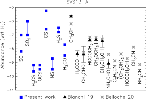
Figure 15: Summary of the abundances with respect to H₂ derived for the hot corino observed towards SVS13-A (N${}_{\rm H_{2}}$ = 3 $\times$ 10²⁴ cm^-2 Chen et al., 2009). Blue points are for the S-species reported in the present paper, while blue triangles (Bianchi et al., 2019a) and grey diamonds (Belloche et al., 2020) are for iCOMs (see Sect. 6.1).

6.2 H₂CS versus H₂CO

One of the main reasons of astrochemical studies of protostellar regions is to understand the chemical composition of the gas where planets start their formation process. As a matter of fact, to understand if the planetary composition has the marks of where planets formed would definitely be a breakthrough result (e.g. Turrini et al., 2021, and references therein). Obviously, several processes are expected to be at work to sculpt the characteristics of planetary atmospheres. Many intermediate steps should intervene between the interstellar chemistry and the planetary chemistry, and consequently, a complete chemical reset cannot be excluded. Whatever is the path leading to planets, the elemental abundance ratios are the root where the atmospheric chemistry is anchored (e.g. Booth & Ilee, 2019; Cridland et al., 2019, and references therein). Together with O, C, N, sulfur is playing a major role in this aspect (e.g. Semenov et al., 2018; Fedele & Favre, 2020; Turrini et al., 2021). With time, the number of S-bearing species around protoplanetary disks is definitely increasing. First, several detections of CS and SO has been reported (e.g. Dutrey et al., 1997, 2017; Fuente et al., 2010; Guilloteau et al., 2013, 2016; Pacheco-Vázquez et al., 2016). More recently, thanks to the advent of ALMA, also H₂S, H₂CS have been imaged towards disk around Class I/II objects showing rings and gaps (Phuong et al., 2018; Le Gal et al., 2019; Codella et al., 2020; Loomis et al., 2020). These findings allow us to compare what we found for the Class I SVS13-A with more evolved star forming regions, namely Class I/II (10⁵–10⁶ yr old).

In this context, as recently remarked by Fedele & Favre (2020), the abundance ratio between H₂CS and H₂CO could be used to investigate the S/O abundance ratio provided that both molecules in the gas-phase are mainly formed by reacting O or S with the methyl group CH₃. In order to estimate [H₂CS]/[H₂CO] in SVS13-A, we used the emission of the o–H₂CO(6_1,5–6_1,6) transition at 101332.991 MHz (E_u = 88 K; from the Cologne Database for Molecular Spectroscopy (CDMS, Müller et al., 2001, 2005). falling in the present Setup 6 at 3mm. Figure 16 reports the H₂CO spatial distribution as well as the spectrum extracted at the peak emission, both perfectly consistent with that of H₂CS as observed with the same spatial and spectral resolution (see Figs. 10 and 11). We then adopted the same size and kinetic temperature range inferred for H₂CS (see Table 2), the ortho/para ratio equal to 3 and, assuming LTE conditions, we derived a total column density N${}_{\rm H_{2}CO}$ = 2-8 $\times$ 10¹⁷ cm^-2. The [H₂CS]/[H₂CO] ratio is then between 9 $\times$ 10^-4 and 2 $\times$ 10^-2.

The present values obtained for a Class I object can be compared with other measurements obtained from interferometric observations sampling Solar System scales around protostars at different evolutionary stages:

• the prototypical Class 0 hot corino IRAS 16293-2422B as revealed with ALMA on a 60 au scale (PILS project: Jørgensen et al., 2016; Persson et al., 2018; Drozdovskaya et al., 2018, 2019): 7 $\times$ 10^-4;

• late Class I or II protoplanetary disks as imaged with ALMA on a 40 au scale (ALMA-DOT project: Podio et al., 2020a; Codella et al., 2020; Garufi et al., 2021): 0.1–0.2 (HL Tau), and 0.4–0.7 (IRAS 04302+2247).

The comparison suggests an increase with time of the [H₂CS]/[H₂CO] ratio in the gaseous compositions around stars by more than one order of magnitude. Obviously, we cannot quantify [S]/[O] from [H₂CS]/[H₂CO] given the complexity of the overall S and O chemistry, but the present findings suggest that [S]/[O] could change along the Sun-like star forming process.

Finally, we inspected what has been measured with the ROSINA spectrometer towards the comet 67P/Churyumov-Garasimenko (C-G) in the context of the ESA Rosetta space mission Rubin et al. (2020). ROSINA derived the chemical composition of the volatiles in the coma, reporting the H₂CS and H₂CO abundance with respect to water. The corresponding [H₂CS]/[H₂CO] ratio ranges in the 7 $\times$ 10^-4 – 4 $\times$ 10^-2 range, i.e. a quite wide spread which does not allow us to verify if a relic of the early stages of our Solar System supports the tentative [H₂CS]/[H₂CO] dependence on time from Class 0 to Class II objects. Clearly, more measurements are needed to perform a statistical study.

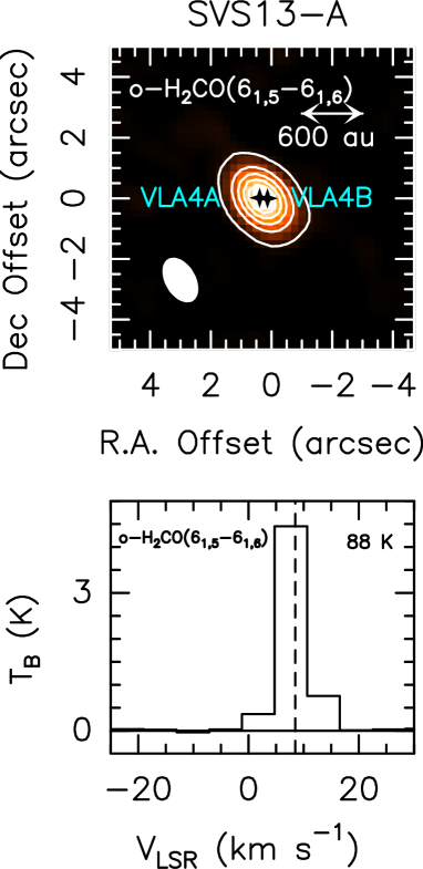
Figure 16: Upper panel: Spatial distribution of the SVS13-A region obtained using the o–H₂CO(6_1,5–6_1,6) emission. The whole velocity emitting region has been used (from –5 km s^-1 to +20 km s^-1). The angular offsets are relative to the phase center (see Sect. 2). First contour and steps are, respectively, 5$\sigma$ (25 mJy km s^-1), and 20$\sigma$, respectively. The filled ellipse shows the synthesised beam (HPBW): 1$\aas@@fstack{\prime\prime}$6 $\times$ 1$\aas@@fstack{\prime\prime}$1 (PA= 41^∘). The black crosses indicate the positions of the VLA4A and VLA4B sources as imaged using the VLA array by Tobin et al. (2018). Lower panel: Observed o–H₂CO(6_1,5–6_1,6) spectrum (in T_B scale, see Table 1) extracted at the emission peak: $\alpha_{2000}$ = 03^h29^m03^s.75, $\delta_{2000}$ = +31^∘16^′03^′′.8. The upper level energy is reported. The vertical dashed line stands for the ambient LSR velocity (+8.6 km s^-1, Chen et al. (2009)).

6.3 NS versus NS⁺

The cation NS⁺ has been very recently discovered in interstellar space using IRAM 30-m observations in the mm-spectral window of a sample of low-mass star-forming regions (Cernicharo et al., 2018). More specifically, NS⁺ has been revealed towards cold molecular clouds and prestellar cores as well as in shocked protostellar regions and in the direction of hot corinos (e.g. NGC1333-IRAS4A). Cernicharo et al. (2018) derived the NS/NS⁺ ratio, lying in the 30–50 range, which has been modelled adopting the following chemical routes (see e.g. Agúndez & Wakelam, 2013): NS is formed by reaction of SH with N or of NH with S, while NS⁺ is formed when the atomic nitrogen reacts with the SO⁺ and SH⁺ ions. On the other hand, both NS and NS⁺ should be destroyed via reactions with the O, N, or C atoms. NS⁺ should go first through dissociative recombination. Cernicharo et al. (2018) fit the observations by using a relatively cold gas, even for the NGC1333-IRAS4A region (T_kin $\simeq$ 30 K), which in turn means that NS⁺ is not released in the hot corino, but instead from a more extended molecular envelope.

In the present SOLIS observations of SVS13-A, NS is clearly tracing the protostellar region with a source size less than 100 au, then it is plausibly emitted in the hot corino (see Fig. 12). In fact, in Sect. 4 we derived the NS column density by assuming a kinetic temperature in the 50–300 K range.

Interestingly, the present SOLIS NOEMA setup is covering (with a $\sim$ 1$\aas@@fstack{\prime\prime}$3 spatial resolution) the frequency of the NS⁺(2–1) line (100198.55 GHz), characterised by E_u = 7 K, $S\mu^{2}$ = 9 D² (Cernicharo et al., 2018). However, this line was not detected and only an upper limit on NS⁺ column density can be derived by assuming the same emitting size as well as the same kinetic temperatures adopted for the NS analysis (see Table 2). The 3$\sigma$ upper limit on the velocity integrated emission is 1 K km s^-1, which in turn allows us to fix an upper limit on N${}_{\rm NH^{+}}$ $\leq$ 8 $\times$ 10¹⁴ cm^-2. In summary, we can derive N(NS)/N(NS⁺) $\geq$ 10, a number in agreement with those reported by Cernicharo et al. (2018), in particular for the NGC1333-IRAS4A hot corino ($\sim$ 40). Note that these findings are also consistent with the inspection of the spectra of the IRAM 30-m ASAI Legacy (Lefloch et al., 2018), which provides an unbiased spectral survey at 1, 2, and 3mm of SVS13-A. ASAI covered not only the NS⁺(2-1) line, but also the $J$ = 3–2 and 5–4 ones, at 150295.607 MHz and 250481.463 MHz, respectively (Cernicharo et al., 2018). No detection has been found, providing an upper limit on the NS⁺ column density of a few 10¹⁴ cm^-2, similarly to what was obtained with NOEMA SOLIS. The present findings, providing the first constraint on the N(NS)/N(NS⁺) ratio based on interferometric data, call for a comparison with predictions from astrochemical modelling at work at kinetic temperatures typical of hot corinos ($\geq$ 100 K).

6.4 SO versus SO₂

The importance of the SO₂ over SO abundance ratio in star forming regions has been discussed since the end of the last century. The starting assumption was that H₂S is the main S-bearing species in the dust mantles. As a consequence, the injection of the material frozen on ices due either to thermal heating (hot cores, hot corinos) or due to sputtering (shocks), or even for chemical desorption caused by the excess energy of an exothermic reaction (Oba et al., 2018), increases the H₂S abundance in the gas-phase, which in turn forms first SO and successively SO₂ (e.g. Pineau des Forets et al., 1993; Charnley et al., 1997; Hatchell et al., 1998). As a result, [SO₂]/[SO] has been proposed to be a chemical clock to date the evaporation/sputtering process. However, successive attempts to apply this tool in young ($\geq$ 10³ yr) shocked regions did not result to be efficient (Codella et al., 1999; Wakelam et al., 2004a; Codella et al., 2005) given all the uncertainties associated with the S-chemistry starting from the still open question on the main S-bearing species frozen on ices (e.g. Laas & Caselli, 2019; Taquet et al., 2020, and references therein). On the other hand, a Kitt Peak single-dish (HPBW = 43$\arcsec$) survey of Class 0 and Class I hot corinos (10⁴–10⁵ yr) by Buckle & Fuller (2003) suggested an evolutionary trend, with [SO₂]/[SO] $\simeq$ 0.1 for Class 0 and [SO₂]/[SO] $\simeq$ 0.4 for Class I.

Moving to interferometric observations, the present dataset shows for the Class I SVS13-A target [SO₂]/[SO] $\sim$ 10, a value larger than what measured with ALMA towards the Class 0 IRAS16293-2422 hot corino (PILS: Drozdovskaya et al., 2018, 2019): [SO₂]/[SO] ratios $\sim$ 3. Both measurements are higher than what measured using IRAM-NOEMA (in the SOLIS context) of the young shocked regions L1157 and L1448 outflows: [SO₂]/[SO] $\simeq$ 0.2 (NGC1333-IRAS4A Taquet et al., 2020), and 0.1–0.3 (L1157 Feng et al., 2020). In conclusion, these recent findings support the use the [SO₂]/[SO] ratio to date gas enriched in sulphur around protostars, using high-spatial interferometric images to disentangle contributions due to different physical components.

6.5 On the sulfur budget in SVS13-A

The recent results by Kama et al. (2019) and Shingledecker et al. (2020) indicates that a large fraction ($\sim$ 90%) of sulphur in dense star forming regions is in very refractory forms such as FeS or S₈. In this context, in order to evaluate the sulfur budget in the Class I SVS13-A hot corino, we need an estimate of the abundance of H₂S, which, as reported in the Sect. 1, is postulated to be a major S-bearing molecule on dust mantles. Unfortunately, the NOEMA SOLIS spectral windows do not cover H₂S line frequencies. However, the H₂S column density can be measured using the line of the para 2_2,0–2_1,1 transition observed at 1.4mm in the context of the IRAM 30-m ASAI Large Program (Lefloch et al., 2018). The line is emitting at 216710.4365 MHz: the HPBW is 11$\arcsec$ and the energy of the upper level is quite high, 84 K . This combination minimises the contaminations expected from the cold envelope with respect to the SVS13-A hot corino, and excludes any possible contribution due to SVS13-B (see Fig. 1). Figure 17 reports the observed spectra, with the p–H₂S(2_2,0–2_1,1) profile peaking at +8.1(0.1) km s^-1, with a FWHM line width equal to 3.2(0.1) km s^-1, and an integrated area (in T_MB scale) of 534(14) mK km s^-1. Given S$\mu^{2}$ = 2.1 D², assuming LTE conditions, an emitting size equal to 0$\aas@@fstack{\prime\prime}$3 and a temperature range of 50–300 K (as for the other S-species here imaged by NOEMA), an ortho/para ratio equal to 3, we obtain a total column density of 0.5–1 $\times$ 10¹⁸ cm^-2. Assuming again N${}_{\rm H_{2}}$ = 3 $\times$ 10²⁴ cm^-2 (Chen et al., 2009), the H₂S abundance results to be 2–4 $\times$ 10^-7. Table 2 and Fig. 15 summarises the column density and abundances of the S-bearing molecules observed in the SVS13-A hot corino. Overall, if we take all of them into account we reach [S]/[H] = 3.0 $\times$ 10^-7 – 3.8 $\times$ 10^-6, i.e. 2%–17% of the Solar System [S]/[H] value (1.8 $\times$ 10^-5; Anders & Grevesse, 1989). Obviously, not all the S-species observed around low-mass protostars have been revealed in the present survey, missing mainly CCS as well as the SO⁺ and HCS⁺ ions. However, we can reasonably assume that the contribution due to CCS (a standard envelope tracer), and the SO⁺ and HCS⁺ ions (two orders of magnitude less abundant than CS in the warm shocked gas in the L1157 outflow Podio et al. (2014)) do not significantly contribute to the total S budget in SVS13-A.

The present measurements can be compared with what obtained in surveys of other prototypical regions associated with Sun-like star-forming regions:

• the Taurus dark cloud TMC 1 has been recently investigated in the context of the GEMS project (Fuente et al., 2019) using the IRAM 30-m and Yebes 40-m antennas in CS, SO, and HCS⁺ (plus rarer isotoplogues of these molecules). The authors found a strong sulfur depletion both in the traslucent low-density phase (where [S]/[H] is 2%–12% of the Solar System one, very similar to what is found in SVS13-A) and in the dense core (where this percentage falls down to 0.4%). Additional GEMS H₂S observations reported by Navarro-Almaida et al. (2020) did not significantly change these results;

• the L1689N star forming region, hosting the well known Class 0 hot corinos IRAS16293-2422A and B has been sampled using SO, and SO₂, and H₂S as observed by Wakelam et al. (2004b) with the IRAM 30-m single-dish. The authors estimate, for the hot corino region, the [S]/[H] ratio to be $\sim$ 8% of the Solar System value. Successively, in the context of the PILS Large Program (Jørgensen et al., 2016), Drozdovskaya et al. (2018, 2019) report the census of S-bearing species as observed with ALMA towards the hot corino IRAS16293-2422B (SO, SO₂, H₂S, CS, H₂CS, and CH₃SH). Assuming an H₂ column density of 10²⁵ cm^-2 derived in the PILS context by (Jørgensen et al., 2016), the [S]/[H] ratio is then $\sim$ 1% of the Solar System measurement;

• Holdship et al. (2019) measured the sulfur budget in the $\sim$ 100 K shocked regions associated with the protostellar L1157 jet. In this case, the sampled region is chemically enriched due to sputtering and shuttering induced by a shock with a velocity of $\simeq$ 20–40 km s^-1 (e.g. Flower et al., 2010; Viti et al., 2011). For the bright L1157-B1 shock Holdship et al. (2019) report [S]/[H] $\sim$ 10% of the Solar System, a value in agreement with what found in SVS13-A.

Figure 17: Spectrum of the p–H₂S(2_2,0–2_1,1) line (in T_MB scale) as observed towards SVS13-A at 1.4mm using the IRAM 30-m antenna. Transition and corresponding upper level energy are reported. The HPBW is also indicated. The vertical dashed line stands for the ambient LSR velocity (+8.6 km s^-1, Chen et al. (2009)).

In summary, the measurements of percentage of the [S]/[H] value with respect to the Solar System value are: 0.4% (dense core), 1%-8% (Class 0 object), 2%-17% (Class I object), 10% (shock). Obviously, these estimates are strongly dependent on the uncertainties associated with the adopted H₂ column densities. For instance Jørgensen et al. (2016) use N(H₂) = 10²⁵ cm^-2 for IRAS16293-2422B, while Bianchi et al. (2019a) and Belloche et al. (2020) adopt 3 $\times$ 10²⁴ cm^-2 for SVS13-A. With these caveats in mind, we can speculate that (i) the increase of S-bearing molecules in the gas-phase due to thermally evaporation in a Class 0 hot corino seems to keep constant also in the more evolved Class I stage; (ii) the enrichment of sulfuretted molecules (with respect to dense cold clouds) due to thermal evaporation seems to be quantitatively the same than that in shocks, where sputtering rules.

7 Summary and conclusions

In the context of the IRAM NOEMA SOLIS Large Program we observed the SVS13-A Class I object at both 3mm (beam $\simeq$ 1$\aas@@fstack{\prime\prime}$5) and 1.4mm (beam $\simeq$ 0$\aas@@fstack{\prime\prime}$6) in order to obtain a census of the S-bearing species. The main results can be summarised as follows:

• We obtained 32 images of emission lines of ³²SO, ³⁴SO, C³²S, C³⁴S, C³³S, OCS, H₂C³²S, H₂C³⁴S, and NS, sampling $E_{\rm u}$ up to 244 K. The low-excitation (9 K) SO is peaking towards SVS13-A. This emission traces also the molecular envelope and the low-velocity outflow emission driven by SVS13-A. SO is also imaging the collimated high-velocity (up to 100 km s^-1 shifted with respect to the systemic velocity) jet driven by the nearby SVS13-B Class 0. In general, the molecular envelope contributes to the low-excitation (less than 40 K) SO and CS emission. Conversely, all the rest of the observed species and transitions show a compact emission around the SVS13-A coordinates indicating the inner $\sim$ 100 au protostellar region.

• The non-LTE LVG analysis of SO, SO₂, and H₂CS indicates a hot corino origin. The emitting size is about 90 au (SO), 60 au (SO₂), and 120 au (H₂CS). For SO, we have $T_{\rm kin}$ $\geq$ 150 K, and $n_{\rm H_{2}}$ $\geq$ 6 $\times$ 10⁶ cm^-3. The analysis of SO₂ leads $T_{\rm kin}$ $\simeq$ 100–300 K, and $n_{\rm H_{2}}$ $\geq$ 5 $\times$ 10⁶ cm^-3. Finally, for H₂CS, $T_{\rm kin}$ $\geq$ 50 K, and $n_{\rm H_{2}}$ $\geq$ 10⁵ cm^-3. For OCS we used the rotation diagram approach using LTE obtaining a $T_{\rm rot}$ of 120$\pm$50 K, consistent with the temperatures expected for a hot corino.

• The bright emission from S-bearing molecules is confirmed to arise from the SVS13-A hot corino, where the iCOMs, previously imaged, are abundant De Simone et al. (2017); Bianchi et al. (2019a); Belloche et al. (2020). The abundances of the sulphuretted species are in the following ranges: 0.3–6 $\times$ 10^-6 (CS), 0.7–10 $\times$ 10^-7 (SO), 1– 10 $\times$ 10^-7 (SO₂), a few 10^-10 (H₂CS and OCS), and 10^-10–10^-9 (NS).

• Also NS is tracing a region with a size less than 100 au. We constrain for the first time the N(NS)/N(NS⁺) using interferometric observations: $\geq$ 10. This is in agreement with what is previously reported for the NGC1333-IRAS4A hot corino by Cernicharo et al. (2018) using single-dish measurements, supporting that NS⁺ is mainly formed in the extended envelope.

• Once measured using the NOEMA array, the [SO₂]/[SO] ratio towards SVS13-A is $\sim$ 10, a value slightly larger (by a factor 3) than what measured with ALMA towards the Class 0 IRAS16293-2422B hot corino (PILS: Drozdovskaya et al., 2018, 2019). This is clearly not enough to support the use of the [SO₂]/[SO] as chemical clock. However, after several unsuccessful attempts done in the past using observations sampling gas on large scales (mainly using single-dish antennas), the present measurements suggest to verify the use of [SO₂]/[SO] as chemical clock, but sampling the inner 100 au around the protostars.

• Considering that in the gas-phase H₂CS and H₂CO (i) are mainly formed by reacting O or S with the methyl group CH₃, and (ii) they are among the fews species detected from protostars to protoplanetary disks, we derived their abundance ratio in SVS13-A, obtaining 0.9 $\times$ 10^-3 – 2 $\times$ 10^-2. The comparison between the few interferometric observations sampling Solar System scales (IRAS 16293-2422B, SVS13-A, HL Tau, and IRAS 04302+2247) suggests an increase with time of the [H₂CS]/[H₂CO] ratio in the gaseous compositions around stars by more than one order of magnitude. It is then tempting to speculate that [S]/[O] could vary along the Sun-like star forming process.

• The estimate of the [S]/[H] budget in SVS13-A is 2%-17% of the Solar System value (1.8 $\times$ 10^-5). This number is consistent with what was previously measured towards Class 0 objects (1%-8%). As a matter of fact, it seems that the enrichment of the S-bearing molecules in Class 0 hot corinos (with respect to dense and cold clouds) remain in the Class I stage.

To conclude, the present results are in agreement with the results reported by Kama et al. (2019), who analysed a sample of young stars photospheres concluding that 89%$\pm$8% of elemental sulfur in their disks is locked in refractory form. Kama et al. (2019) conclude that the main S-carrier in the dust has to be more refractory than water, suggesting sulfide minerals such as FeS. Note also that recently (Shingledecker et al., 2020) have shown that radiation chemistry converts a large fraction of S in allotropic form, in particular S₈, which cannot be detected (except for possible desorption products due to photo-processes or shocks, such as S₂, S₃ and S₄, as also detected in the coma of the 67P/Churyumov-Gerasimenko comet (Calmonte et al., 2016). Indeed, this is supported by the fact that even in a shocked region such as L1157-B1, associated with both C and J-shocks (Benedettini et al., 2012) and indeed rich in water (H₂O/H₂ = 10^-4; Busquet et al., 2014), the [S]/[H] ratio is not significantly larger than what is found in both Class 0 and Class I hot corinos.

Appendix A Comparison between NOEMA-SOLIS and IRAM 30m-ASAI

Figures A.1 and A.2 show the comparison between the IRAM 30-m 1.4mm and 3mm spectrum obtained in the context of the ASAI Large Program Lefloch et al. (2018) and the spectra derived by integrating the emission in the NOEMA-SOLIS images in a region equal to the HPBW of the IRAM 30-m. The output is clearly different, with the single-dish observations collecting not only the emission imaged with NOEMA (LAS $\simeq$ 8$\arcsec$–9$\arcsec$), but also the large scale structure (e.g. molecular envelope around SVS13-A, extended outflow.). More specifically, Figs. A.3 and A.4 report zoomed-in portions of the 3mm and 1.4mm spectra to enlight lines of selected S-bearing molecules. The comparison confirms that, as expected, the NOEMA-SOLIS maps are well suited to image hot corinos. A particular case is represented by the SO single-dish spectra, which are collecting a considrable amount of flux due to extnded emission. On the other hand, the lines due to e.g. SO₂ and H₂CS are less affected by emission filtering.

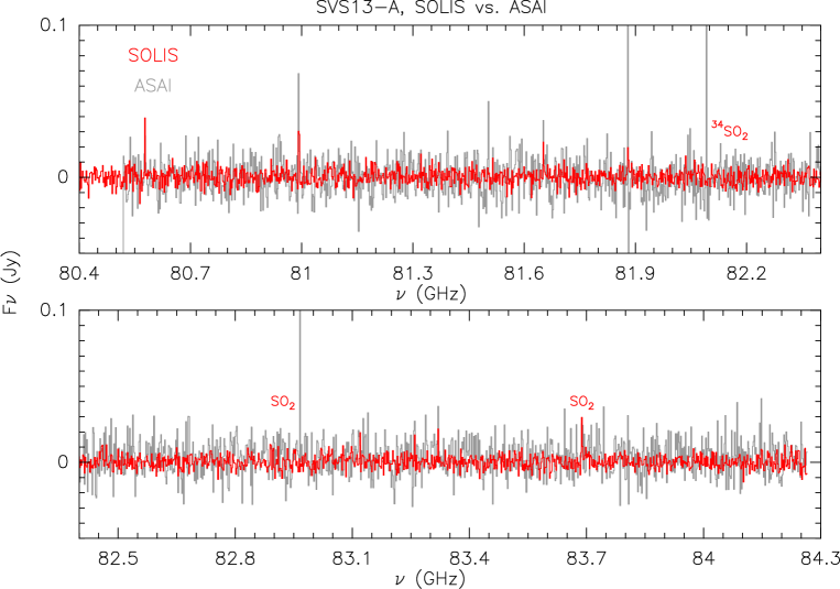
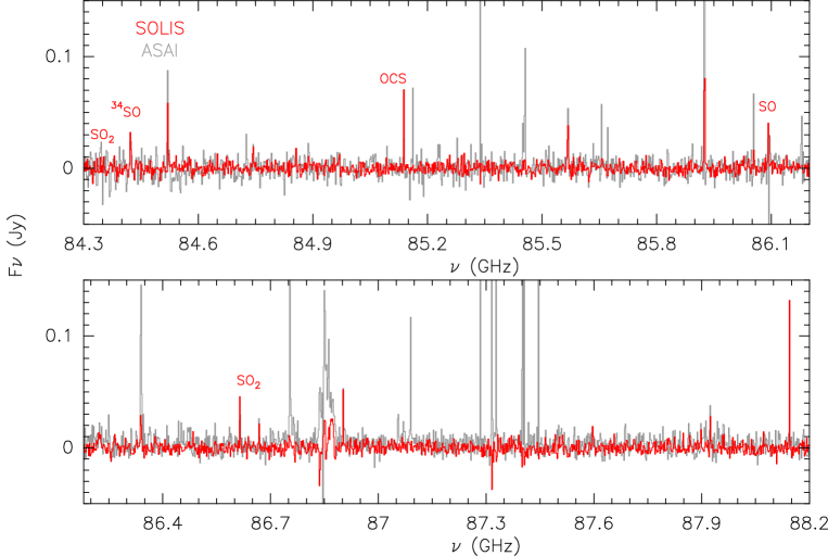
Figure 18: Comparison (in flux density scale) of the 3mm spectrum as observed using the IRAM 30-m antenna (grey; in the ASAI LP context Lefloch et al. (2018)) and that extracted from the present NOEMA SOLIS maps (red) from a circular region equal to the IRAM 30-m HPBW (24$\arcsec$ at 104 GHz, 31$\arcsec$ at 80 GHz). The ASAI spectrum has been smoothed to match the SOLIS velocity resolution (2 MHz, see Sect. 2). Red labels indicate the S-bearing species analysed in this paper (see Table 1).

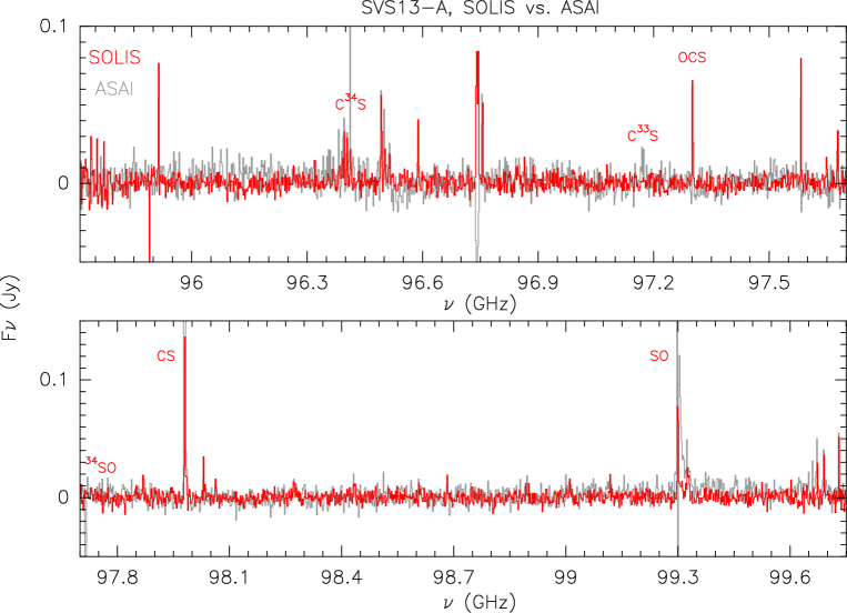
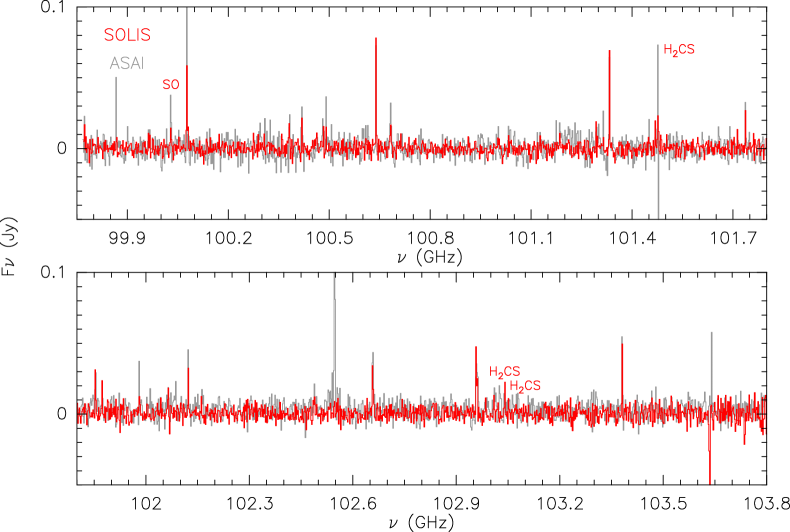
Figure 18: Continued. Comparison (in flux density scale) of the 3mm spectrum as observed using the IRAM 30-m antenna (grey; in the ASAI LP context Lefloch et al. (2018)) and that extracted from the present NOEMA SOLIS maps (red) from a circular region equal to the IRAM 30-m HPBW (24$\arcsec$ at 104 GHz, 31$\arcsec$ at 80 GHz). The ASAI spectrum has been smoothed to match the SOLIS velocity resolution (2 MHz, see Sect. 3). Red labels indicate the S-bearing species analysed in this paper (see Table 1).

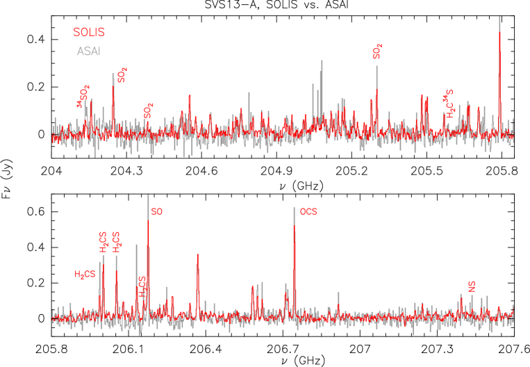
Figure 19: Comparison (in flux density scale) of the 1.4mm spectrum as observed using the IRAM 30-m antenna (grey; in the ASAI LP context Lefloch et al. (2018)) and that extracted from the present NOEMA SOLIS maps (red) from a circular region equal to the IRAM 30-m HPBW (12$\arcsec$). The ASAI spectrum has been smoothed to match the SOLIS velocity resolution (2 MHz, see Sect. 3). Red labels indicate the S-bearing species analysed in this paper (see Table 1).

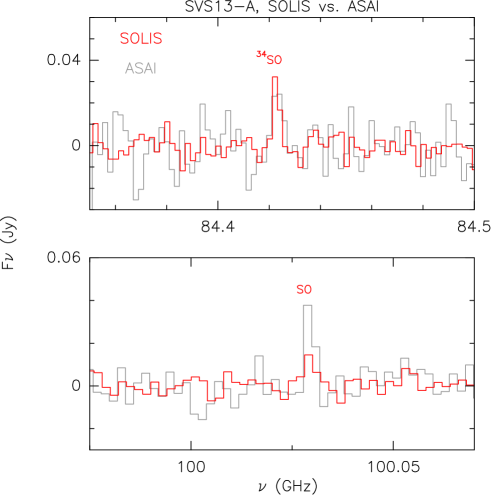
Figure 20: Zoom-in of Fig. A.1 to enlight selected emission lines of S-bearing species: comparison (in flux density scale) of the 3mm spectrum as observed using the IRAM 30-m antenna (grey; in the ASAI LP context Lefloch et al. (2018)) and that extracted from the present NOEMA SOLIS maps (red) from a circular region equal to the IRAM 30-m HPBW (25$\arcsec$ at 100 GHz, 29$\arcsec$ at 84 GHz). The ASAI spectrum has been smoothed to match the SOLIS velocity resolution (2 MHz, see Sect. 3). Red labels indicate the S-bearing species analysed in this paper (see Table 1).

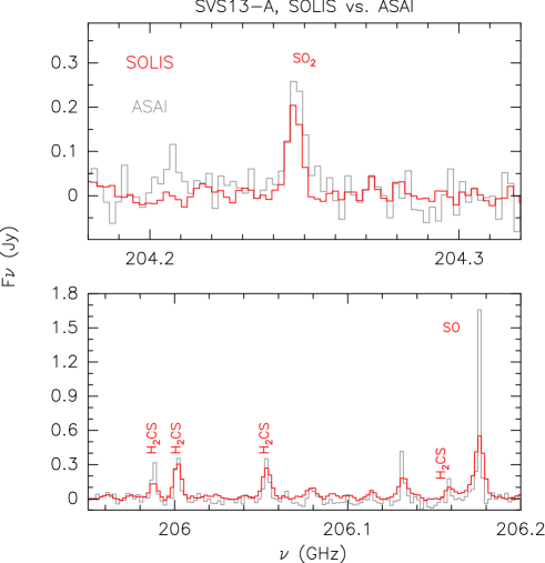
Figure 21: Zoom-in of Fig. A.2 to enlight selected emission lines of S-bearing species: comparison (in flux density scale) of the 1.4mm spectrum as observed using the IRAM 30-m antenna (grey; in the ASAI LP context Lefloch et al. (2018)) and that extracted from the present NOEMA SOLIS maps (red) from a circular region equal to the IRAM 30-m HPBW (12$\arcsec$). The ASAI spectrum has been smoothed to match the SOLIS velocity resolution (2 MHz, see Sect. 3). Red labels indicate the S-bearing species analysed in this paper (see Table 1).