Vacuum currents in partially compactified Rindler spacetime
with an application to cylindrical black holes

Abstract

The vacuum expectation value of the current density for a charged scalar field is investigated in Rindler spacetime with a part of spatial dimensions compactified to a torus. It is assumed that the field is prepared in the Fulling-Rindler vacuum state. For general values of the phases in the periodicity conditions and the lengths of compact dimensions, the expressions are provided for the Hadamard function and vacuum currents. The current density along compact dimensions is a periodic function of the magnetic flux enclosed by those dimensions and vanishes on the Rindler horizon. The obtained results are compared with the corresponding currents in the Minkowski vacuum. The near-horizon and large-distance asymptotics are discussed for the vacuum currents around cylindrical black holes. In the near-horizon approximation the lengths of compact dimensions are determined by the horizon radius. At large distances from the horizon the geometry is approximated by a locally anti-de Sitter spacetime with toroidally compact dimensions and the lengths of compact dimensions are determined by negative cosmological constant.

Keywords: Topological Casimir effect, Rindler spacetime, vacuum currents, Fulling-Rindler vacuum

1 Introduction

In quantum field theory the vacuum state, in general, depends on the choice of the complete set of mode functions used for the expansion of the field operator (see, for instance, [1]). Among the most known examples are the Minkowski and Fulling-Rindler (FR) vacua in Minkowski spacetime. The first one is realized by the plane-wave modes most frequently used in considerations of quantum field-theoretical effects on background of flat spacetime. The FR vacuum [2] corresponds to the quantization of fields in the reference frame with the coordinate lines corresponding to the worldlines of uniformly accelerated observers (Rindler coordinates). On the base of the equivalence principle, we can expect that properties of quantum fluctuations in the FR vacuum will have common qualitative features with those for vacuum states of quantum fields in classical gravitational backgrounds. In particular, the Rindler metric is the leading approximation of the near-horizon geometry for most black holes. A better understanding of quantum vacuum effects in Rindler spacetime serves as a handle in considerations of more complicated background geometries like Schwarzschild. Another motivation for the study of the properties of the FR vacuum is related to the conformal connection of the Rindler metric tensor to the metric tensors of de Sitter spacetime and of the Friedmann-Robertson-Walker spacetime with negative spatial curvature [1]. By using these conformal relations, the expectation values of local physical observables for conformally invariant fields in those spacetimes are obtained from the Rindler expectation values by conformal transformations. Rindler observers in anti-de Sitter (AdS) spacetime and the related AdS/CFT correspondence have been discussed in [3]-[8].

Among the interesting topics in the investigations of the properties for a given vacuum state is the influence of background topology and of boundaries having different physical nature. The corresponding quantum field-theoretical effects are known under the general name Casimir effect (for reviews see [9]-[12]). The influence of uniformly accelerated planar boundaries on both the local and global characteristics of the FR vacuum has been studied in [13]-[19]. The bulk and surface Casimir densities for a spherical boundary in Rindler-like spacetimes were discussed in [20, 21]. In the present paper we consider the effects of nontrivial topology on the expectation value of the current density for a charged scalar field in a locally Rindler spacetime with a part of spatial dimensions compactified to a torus. In appendix B we show that the corresponding metric tensor describes the near-horizon geometry of cylindrical black holes (black strings in another terminology, for geometrical properties see [22]-[28] and references therein). The field-theoretical models with compact dimensions appear in a large number of physical problems including the Kaluza-Klein-type theories, supergravity and string theories, and effective field-theoretical models in condensed matter physics (for example, the Dirac model in the long-wavelength description of graphene nanotubes and nanoloops). The topological Casimir effect has been considered previously as a stabilization mechanism in theories with extra spatial dimensions and as a source of the dark energy driving the accelerated expansion of the universe. In addition, the vacuum expectation values (VEVs) of the current densities along compact dimensions may serve as a source for large scale magnetic fields in models with extra dimensions.

The paper is organized as follows. In the next section we describe the geometry of the problem and present the complete set of scalar modes. The properties of the vacuum state are encoded in two-point functions and in Section 3 we evaluate the Hadamard function for a general number of compact and uncompact dimensions. By using the expression for the Hadamard function, the VEV of the current density along compact dimensions is investigated in Section 4. The main results of the paper are summarized in Section 5. In Appendix A, a representation of the Hadamard function for the Minkowski vacuum is provided that is used in the main text for the investigation of the effects induced by acceleration. In Appendix B we demonstrate that the near-horizon geometry of cylindrical black holes is approximated by Rindler spacetime with toral spatial dimensions.

2 Scalar field modes in Rindler spacetime with compact dimensions

We start by the description of the background geometry. The latter is given by $(D+1)$-dimensional locally Rindler line element

$$ds^{2}=\xi^{2}d\tau^{2}-d\xi^{2}-\sum_{i=2}^{D}\left(dx^{i}\right)^{2},$$ (1)

with the Rindler coordinates $x^{\mu}=\left(x^{0}=\tau,x^{1}=\xi,\mathbf{x}_{p},\mathbf{x}_{q}\right)$ and $0<\xi<\infty$. The $p$-dimensional subspace with Cartesian coordinates $\mathbf{x}_{p}=(x^{2},...,x^{p+1})$ has trivial topology $R^{p}$ with $-\infty<x^{l}<\infty$ for $l=2,..,p+1$. The $q$-dimensional subspace covered by the coordinates $\mathbf{x}_{q}=(x^{p+2},...,x^{D})$ is compactified to a torus $(S^{1})^{q}$, $q=D-p-1$. In the discussion below the length of the compact dimension $x^{l}$ will be denoted by $L_{l}$ and $0\leqslant x^{l}\leqslant L_{l}$ for $l=p+2,...,D$. Hence, the subspace with the coordinates $(x^{2},x^{3},\ldots,x^{D})$ has spatial topology $R^{p}\times(S^{1})^{q}$. Introducing the coordinates

$$t_{\mathrm{M}}=\xi\sinh\tau,\quad x_{\mathrm{M}}^{1}=\xi\cosh\tau,$$ (2)

in the subspace $(\tau,\xi)$, the line element (1) is written in the locally Minkowskian form

$$ds^{2}=\eta_{\mu\nu}dx_{\mathrm{M}}^{\mu}dx_{\mathrm{M}}^{\nu},$$ (3)

where $\eta_{\mu\nu}=\mathrm{diag}(1,-1,\ldots,-1)$ is the Minkowski metric tensor and $x_{\mathrm{M}}^{0}=t_{\mathrm{M}}$, $x_{\mathrm{M}}^{\mu}=x^{\mu}$ for $\mu=2,\ldots,D$. As seen from (2), the coordinates $x^{\mu}$ cover the right Rindler wedge $x_{\mathrm{M}}^{1}>|t_{\mathrm{M}}|$. The worldline for given $(\xi,x^{2},\ldots,x^{D})$ corresponds to an observer with constant proper acceleration $1/\xi$. The proper time for that observer is expressed in terms of the dimensionless time coordinate $\tau$ as $t=\xi\tau$.

Having specified the geometry we turn to the field content. We consider a quantum charged scalar field $\varphi(x)$. Assuming the presence of an external classical gauge field with the vector potential $A_{\mu}$, the field equation reads

$$\left(g^{\mu\nu}D_{\mu}D_{\nu}+m^{2}\right)\varphi=0,$$ (4)

where $D_{\mu}=\nabla_{\mu}+ieA_{\mu}$, the operator $\nabla_{\mu}$ stands for the standard covariant derivative in coordinates $x^{\mu}=\left(\tau,\xi,\mathbf{x}_{p},\mathbf{x}_{q}\right)$ and $e$ is the charge of the field quanta. Note that the background geometry is flat and the equation (4) is valid for general case of the curvature coupling parameter. The spatial topology is nontrivial and for the theory to be defined in addition to the field equation we need to specify the periodicity conditions on the field operator along compact dimensions. In what follows generic quasiperiodic conditions

$$\varphi(t,\xi,\mathbf{x}_{p},\mathbf{x}_{q}+L_{l}\mathbf{e}_{l})=e^{i\alpha_{l}}\varphi(t,\xi,\mathbf{x}_{p},\mathbf{x}_{q}),$$ (5)

will be imposed for $l=p+2,\ldots,D$. In (5), $\mathbf{e}_{l}$ is the unit vector along the compact dimension $x^{l}$ and the constant phases $\alpha_{l}$ can differ for different directions. The special cases of untwisted and twisted fields, most frequently considered in the literature, are realized by the choice $\alpha_{l}=0$ and $\alpha_{l}=\pi$, respectively, for all values of $l=p+2,\ldots,D$.

For an external gauge field $A_{\mu}$ we will take a simple configuration with the only nonzero components $A_{\mu}=\mathrm{const}$ along compact dimensions $x^{\mu}$, $\mu=p+2,\ldots,D$. By making use of the gauge transformation

$$\varphi^{\prime}(x)=e^{ie\chi}\varphi(x),\;A_{\mu}^{\prime}=A_{\mu}-\partial_{\mu}\chi,$$ (6)

with $\chi=A_{\mu}x^{\mu}$ we get $A_{\mu}^{\prime}=0$ and the vector potential does no enter in the field equation for $\varphi^{\prime}(x)$. However, the gauge transformation modifies the periodicity conditions for the new field as

$$\varphi^{\prime}(t,\mathbf{x}_{p},\mathbf{x}_{q}+L_{l}\mathbf{e}_{l})=e^{i\tilde{\alpha}_{l}}\varphi^{\prime}(t,\mathbf{x}_{p},\mathbf{x}_{q}),$$ (7)

with the new phases

$$\tilde{\alpha}_{l}=\alpha_{l}+eA_{l}L_{l}.$$ (8)

The physical observables depend on the phases $\alpha_{l}$ and on the constant components $A_{l}$ through the gauge invariant combination (8). The effect of a constant gauge field is related to the nontrivial spatial topology and is of the Aharonov-Bohm-type. The consideration below will be presented in terms of the field $\varphi^{\prime}(x)$. Omitting the prime, the corresponding field equation is given by (4) with $D_{\mu}=\nabla_{\mu}$.

The properties of the vacuum state in the problem under consideration are completely determined by the two-point functions. For the evaluation of those functions we will use the representation in the form of the summation over complete set of mode functions. The mode functions realizing the FR vacuum are specified by the energy $\omega$ and the momentum $\mathbf{k}$ and are given by the expression (for quantization of fields in Rindler spacetime with trivial topology see, for example, [1, 29])

$$\varphi_{\omega,\mathbf{k}}^{(\pm)}(x)=C_{\omega,\mathbf{k}}e^{i\mathbf{k}\cdot\mathbf{x}\mp i\omega\tau}K_{i\omega}(\lambda\xi),\;\lambda=\sqrt{k^{2}+m^{2}},$$ (9)

where the upper and lower signs correspond to the positive and negative energy modes, $\mathbf{x}=(\mathbf{x}_{p},\mathbf{x}_{q})$, $k=|\mathbf{k}|$, and $K_{\nu}(x)$ is the modified Bessel function [30]. The momentum $\mathbf{k}$ is decomposed as $\mathbf{k}=(\mathbf{k}_{p},\mathbf{k}_{q})$, with the components $\mathbf{k}_{p}=(k_{2},\ldots,k_{p+1})$ and $\mathbf{k}_{q}=(k_{p+2},\ldots,k_{D})$ corresponding to the uncopmact and compact subspaces (with topologies $R^{p}$ and $(S^{1})^{q}$), respectively. For the components along uncompact dimensions we have $-\infty<k_{n}<+\infty$, $n=2,\ldots,p+1$. The components along the compact dimensions are quantized by the periodicity conditions (7) with the eigenvalues

$$k_{l}=\left(2\pi n_{l}+\tilde{\alpha}_{l}\right)/L_{l},$$ (10)

where $n_{l}=0,\pm 1,\pm 2,\ldots.,$ and $l=p+2,...,D$. Note that the energy $\omega$ in (9) is dimensionless. The energy measured by an observer with proper acceleration $1/\xi$ is expressed as $\omega/\xi$. The mode functions (9) are normalized by the condition

$$\int d{\mathbf{x}}\int_{0}^{\infty}\frac{d\xi}{\xi}\varphi_{\omega,\mathbf{k}}^{(s)}\overset{\leftrightarrow}{\partial}_{\tau}\varphi_{\omega^{\prime},\mathbf{k}^{\prime}}^{(s^{\prime})\ast}=i\delta_{ss^{\prime}}\delta\left(\omega-\omega^{\prime}\right)\delta\left(\mathbf{k}_{p}-\mathbf{k}_{p}^{\prime}\right)\delta_{\mathbf{k}_{q}\mathbf{k}_{q}^{\prime}},$$ (11)

where $\delta_{\mathbf{k}_{q}\mathbf{k}_{q}^{\prime}}=\delta_{n_{p+2},n_{p+2}^{\prime}}....\delta_{n_{D},n_{D}^{\prime}}$. By using the result (see, for example, [31])

$$\int_{0}^{\infty}\frac{dy}{y}\,K_{i\omega}(y)K_{i\omega^{\prime}}(y)=\frac{\pi^{2}\delta\left(\omega-\omega^{\prime}\right)}{2\omega\sinh(\omega\pi)},$$ (12)

for the coefficient in (9) we get

$$|C_{\omega,\mathbf{k}}|^{2}=\frac{\sinh\left(\pi\omega\right)}{(2\pi)^{p}\pi^{2}V_{q}}.$$ (13)

Here and below, for the volume of the compact subspace we use the notation $V_{q}=L_{p+2}....L_{D}$. In the present paper we are interested in the VEV of the current density (for quantum effects in models with toroidally compact dimensions see [32] and references therein)

$$j_{\mu}(x)=ie[\varphi^{\dagger}(x)\partial_{\mu}\varphi(x)-(\partial_{\mu}\varphi^{\dagger}(x))\varphi(x)],$$ (14)

for the field $\varphi(x)$. It can be evaluated by using the two-point function. As such a function in the next section we consider the Hadamard function.

3 Hadamard function

The Hadamard function for a charged scalar field $\varphi(x)$ is defined as the VEV

$$G(x,x^{\prime})=\left\langle 0\right|\varphi(x)\varphi^{\dagger}(x^{\prime})+\varphi^{\dagger}(x^{\prime})\varphi(x)\left|0\right\rangle,$$ (15)

with $\left|0\right\rangle$ being the vacuum state (the FR vacuum in our consideration). Having the mode functions, the Hadamard function for the FR vacuum can be written in the form of the mode sum

$$G(x,x^{\prime})=\int d\mathbf{k}_{p}\int_{0}^{\infty}d\omega\sum_{\mathbf{n}_{q}}\sum_{s=\pm}\varphi_{\mathbf{k}}^{(s)}(x)\varphi_{\mathbf{k}}^{(s)\ast}(x^{\prime}),$$ (16)

where $\mathbf{n}_{q}=(n_{p+2},n_{p+3},\ldots,n_{D})$ and

$$\sum_{\mathbf{n}_{q}}=\sum_{n_{p+2}=-\infty}^{+\infty}\cdots\sum_{n_{D}=-\infty}^{+\infty}.$$ (17)

Substituting the mode functions from (9) we get

$$G(x,x^{\prime})=\frac{2^{1-p}}{\pi^{p+2}V_{q}}\int d{\mathbf{k}}_{p}\,\sum_{\mathbf{n}_{q}}e^{i{\mathbf{k}}\cdot\Delta{\mathbf{x}}}\int_{0}^{\infty}d\omega\sinh(\pi\omega)\cos\left(\omega\Delta\tau\right)K_{i\omega}(\lambda_{\mathbf{k}}\xi)K_{i\omega}(\lambda_{\mathbf{k}}\xi^{\prime}),$$ (18)

where $\Delta{\mathbf{x=x}}-{\mathbf{x}^{\prime}}$, $\Delta\tau=\tau-\tau^{\prime}$ and

$$\lambda_{\mathbf{k}}=\sqrt{\mathbf{k}_{p}^{2}+\mathbf{k}_{q}^{2}+m^{2}},\;\mathbf{k}_{q}^{2}=\sum_{l=p+2}^{D}\left(\frac{2\pi n_{l}+\tilde{\alpha}_{l}}{L_{l}}\right)^{2}.$$ (19)

In order to compare the effects of compactification on the FR and Minkowski vacua let us consider the Hadamard function for the Minkowski vacuum $\left|0\right\rangle_{\mathrm{M}}$ in the locally Minkowski spacetime with the line element (3) and the spatial topology $R^{p+1}\times(S^{1})^{q}$ (for a recent discussion of relations between the Minkowski and Rindler propagators see [33] and references therein). In Appendix A we show that the Minkowskian Hadamard function $G_{\mathrm{M}}(x,x^{\prime})$ is presented in the form

$$G_{\mathrm{M}}(x,x^{\prime})=\frac{2^{1-p}}{\pi^{p+2}V_{q}}\int d\mathbf{k}_{p}\sum_{\mathbf{n}_{q}}e^{i\mathbf{k}\cdot\Delta{\mathbf{x}}}\int_{0}^{\infty}d\omega\,\cosh\left(\pi\omega\right)\cos\left(\omega\Delta\tau\right)K_{i\omega}(\lambda_{\mathbf{k}}\xi)K_{i\omega}(\lambda_{\mathbf{k}}\xi^{\prime}).$$ (20)

This form is convenient for the investigation of the difference between the VEVs in the FR and Minkowski vacua.

By using the representations (18) and (20), the difference of the Hadamard functions is expressed as

$$G(x,x^{\prime})-G_{\mathrm{M}}(x,x^{\prime}) = -\frac{2^{1-p}}{\pi^{p+2}V_{q}}\int d{\mathbf{k}}_{p}\,\sum_{\mathbf{n}_{q}}e^{i{\mathbf{k}}\cdot\Delta{\mathbf{x}}}\int_{0}^{\infty}d\omega\,e^{-\pi\omega}$$ (21)

$$\times\cos\left(\omega\Delta\tau\right)K_{i\omega}(\lambda_{\mathbf{k}}\xi)K_{i\omega}(\lambda_{\mathbf{k}}\xi^{\prime}).$$

For the further transformation of (21) we employ the integral representation [34] (in [34] there is a missprint, instead of $\left(x^{2}+X^{2}\right)/u$ should be $-\left(x^{2}+X^{2}\right)/2u$)

$$K_{\nu}(X)K_{\nu}(x)=\frac{1}{2}\int_{0}^{\infty}dT\int_{0}^{\infty}\frac{du}{u}\cosh\left(\nu T\right)e^{-(xX/u)\cosh T}\exp\left[-\left(\frac{u}{2}+\frac{x^{2}+X^{2}}{2u}\right)\right],$$ (22)

for the product of the modified Bessel functions. Substituting (22) in (21), we first integrate over $\omega$ and then over $u$ and ${\mathbf{k}}_{p}$. This leads to the final result

$$G(x,x^{\prime}) = G_{\mathrm{M}}(x,x^{\prime})-\frac{2^{-p/2}}{\pi^{p/2+1}V_{q}}\sum_{\mathbf{n}_{q}}\omega_{\mathbf{n}_{q}}^{p}e^{i{\mathbf{k}}_{q}\cdot({\mathbf{x}}_{q}-{\mathbf{x}_{q}^{\prime}})}\int_{0}^{\infty}dT\sum_{s=\pm 1}\frac{1}{\left(T-s\Delta\tau\right)^{2}+\pi^{2}}$$ (23)

$$\times f_{p/2}\left(\omega_{\mathbf{n}_{q}}\sqrt{|{\mathbf{x}}_{p}-{\mathbf{x}_{p}^{\prime}}|^{2}+\xi^{2}+\xi^{\prime 2}+2\xi\xi^{\prime}\cosh T}\right),$$

where we have introduced the notations $f_{\nu}(x)=K_{\nu}(x)/x^{\nu}$ and $\omega_{\mathbf{n}_{q}}=\sqrt{\mathbf{k}_{q}^{2}+m^{2}}$. Note that the divergences for $G(x,x^{\prime})$ and $G_{\mathrm{M}}(x,x^{\prime})$ in the coincidence limit $x^{\prime}\rightarrow x$ are the same and the last term in (23) is finite in that limit.

4 Current density

4.1 General expression

Having the Hadamard function we can evaluate the expectation value for the current density (14) in the FR vacuum by using the formula

$$\left\langle 0\right|j_{\mu}(x)\left|0\right\rangle\equiv\left\langle j_{\mu}\right\rangle=\frac{i}{2}e\lim_{x^{\prime}\rightarrow x}(\partial_{\mu}-\partial_{\mu}^{\prime})G(x,x^{\prime}).$$ (24)

First we can see that the VEVs for the charge density and for the components along the uncompact directions vanish, $\left\langle j_{\mu}\right\rangle=0$, $\mu=0,1,\ldots,p+1$. By making use of (24) and the expression (23) of the Hadamard function, for the contravariant component of the current density along the $l$-th compact dimension we get:

$$\langle j^{l}\rangle=\langle j^{l}\rangle_{\mathrm{M}}-\frac{2^{-p/2}e}{\pi^{p/2+1}V_{q}}\sum_{\mathbf{n}_{q}}k_{l}\omega_{\mathbf{n}_{q}}^{p}\int_{0}^{\infty}dx\,\frac{f_{p/2}\left(2\xi\omega_{\mathbf{n}_{q}}\cosh x\right)}{x^{2}+\pi^{2}/4},$$ (25)

where $k_{l}$ is given by (10) and $\langle j^{l}\rangle_{\mathrm{M}}$ is the current density for the Minkowski vacuum. The latter has been investigated in [35]. The corresponding formula is obtained from [35] by the replacement $p\rightarrow p+1$:

$$\langle j^{l}\rangle_{\mathrm{M}}=\frac{4eL_{l}^{2}V_{q}^{-1}}{(2\pi)^{\left(p+3\right)/2}}\sum_{n_{l}=1}^{\infty}n_{l}\sin(n_{l}\tilde{\alpha}_{l})\sum_{\mathbf{n}_{q-1}^{l}}\omega_{\mathbf{n}_{q-1}}^{p+3}f_{\frac{p+3}{2}}(n_{l}L_{l}\omega_{\mathbf{n}_{q-1}}),$$ (26)

where $\mathbf{n}_{q-1}^{l}=(n_{p+2},\ldots,n_{l-1},,n_{l+1},\ldots,n_{D})$ and $\omega_{\mathbf{n}_{q-1}}=\sqrt{\mathbf{k}_{q-1}^{2}+m^{2}}$ with $\mathbf{k}_{q-1}^{2}=\mathbf{k}_{q}^{2}-k_{l}^{2}$. An equivalent expression is given by [35]

$$\langle j^{l}\rangle_{\mathrm{M}}=\frac{2eL_{l}m^{D+1}}{(2\pi)^{(D+1)/2}}\sum_{\mathbf{n}_{q}}n_{l}\sin\left(\mathbf{n}_{q}\cdot\boldsymbol{\tilde{\alpha}}\right)f_{\frac{D+1}{2}}\left(m\sqrt{\sum\nolimits_{i=p+2}^{D}n_{i}^{2}L_{i}^{2}}\right),$$ (27)

with $\mathbf{n}_{q}\cdot\boldsymbol{\tilde{\alpha}}=\sum\nolimits_{i=p+2}^{D}n_{i}\tilde{\alpha}_{i}$. Note that the Minkowskian part is homogeneous. Both the contributions in (25) are odd periodic functions of $\tilde{\alpha}_{l}$ with the period $2\pi$ and even periodic functions of $\tilde{\alpha}_{i}$, $i\neq l$,with the same period. By making use of a gauge transformation similar to (6) with $\chi\left(x\right)=-\sum_{i=p+2}^{D}\alpha_{i}x^{i}/eL_{i}$ we can pass to a new gauge with the fields $(\tilde{\varphi}(x),\tilde{A}_{\mu})$, where $\tilde{A}_{i}=\tilde{\alpha}_{i}/eL_{i}$, $i=p+2,\ldots,D$, and the function $\tilde{\varphi}(x)$ is periodic along compact dimensions. In this gauge, the formal magnetic flux enclosed by the $i$th compact dimension is given as $\tilde{\Phi}_{i}=-\tilde{A}_{i}L_{i}$. The parameter $\tilde{\alpha}_{i}$ is expressed as $\tilde{\alpha}_{i}=-2\pi\tilde{\Phi}_{i}/\Phi_{0}$, where $\Phi_{0}=2\pi/e$ ($2\pi\hbar c/e$ in standard units) is the flux quantum. As seen, the periodicity with respect to $\tilde{\alpha}_{i}$ is translated to a periodicity with respect to the magnetic flux $\tilde{\Phi}_{i}$ with the period of flux quantum.

An alternative expression for the current density $\langle j^{l}\rangle$ in the FR vacuum is obtained by using the formula [35]

$$\sum_{\mathbf{n}}\cos(\mathbf{n}\cdot\boldsymbol{\beta})f_{\nu}(c\sqrt{b^{2}+\sum\nolimits_{i=1}^{r}a_{i}^{2}n_{i}^{2}})=\frac{(2\pi)^{r/2}}{a_{1}\cdots a_{r}c^{2\nu}}\sum_{\mathbf{n}}w_{\mathbf{n}}^{2\nu-r}f_{\nu-\frac{r}{2}}(bw_{\mathbf{n}}),$$ (28)

where $\mathbf{n}=(n_{1},\ldots,n_{r})$, $\boldsymbol{\beta}=(\beta_{1},\ldots,\beta_{r})$, and $w_{\mathbf{n}}^{2}=\sum\nolimits_{i=1}^{r}(2\pi n_{i}+\beta_{i})^{2}/a_{i}^{2}+c^{2}$. By taking the derivative with respect to $\beta_{l}$ from here we find

$$\sum_{\mathbf{n}}\frac{2\pi n_{l}+\beta_{l}}{a_{l}^{2}}w_{\mathbf{n}}^{2\nu-r-2}f_{\nu-\frac{r}{2}-1}(bw_{\mathbf{n}})=\frac{a_{1}\cdots a_{r}c^{2\nu}}{(2\pi)^{r/2}}\sum_{\mathbf{n}}n_{l}\sin(\mathbf{n}\cdot\boldsymbol{\beta})f_{\nu}(c\sqrt{b^{2}+\sum\nolimits_{i=1}^{r}a_{i}^{2}n_{i}^{2}}).$$ (29)

Choosing $r=D-p-1$, $c=m$, $\nu=(D+1)/2$, $\beta_{i}=\tilde{\alpha}_{p+i+1}$ and $a_{i}=L_{p+i+1}$, one gets the formula

$$\sum_{\mathbf{n}_{q}}k_{l}\omega_{\mathbf{n}_{q}}^{p}f_{\frac{p}{2}}(b\omega_{\mathbf{n}_{q}})=\frac{V_{q}L_{l}m^{D+1}}{(2\pi)^{(D-p-1)/2}}\sum_{\mathbf{n}_{q}}n_{l}\sin(\mathbf{n}_{q}\cdot\boldsymbol{\tilde{\alpha}})f_{\frac{D+1}{2}}(m\sqrt{b^{2}+\sum\nolimits_{i=p+2}^{D}L_{i}^{2}n_{i}^{2}}).$$ (30)

By using this relation with $b=2\xi\cosh x$ in (25), the following formula is obtained

$$\langle j^{l}\rangle = \langle j^{l}\rangle_{\mathrm{M}}-\frac{2em^{D+1}L_{l}}{(2\pi)^{(D+1)/2}}\sum_{\mathbf{n}_{q}}n_{l}\sin\left(\mathbf{n}_{q}\cdot\boldsymbol{\tilde{\alpha}}\right)$$ (31)

$$\times\int_{0}^{\infty}\,\frac{dx}{x^{2}+\pi^{2}/4}f_{\frac{D+1}{2}}(m\sqrt{4\xi^{2}\cosh^{2}x+\sum\nolimits_{i=p+2}^{D}L_{i}^{2}n_{i}^{2}}).$$

Note that in this formula we can make the replacement

$$\sum_{\mathbf{n}_{q}}n_{l}\sin\left(\mathbf{n}_{q}\cdot\boldsymbol{\tilde{\alpha}}\right)\rightarrow 2\sum_{n_{l}=1}^{\infty}n_{l}\sin(n_{l}\tilde{\alpha}_{l})\sum_{\mathbf{n}_{q-1}^{l}}\cos\left(\sum\nolimits_{i=p+2,\neq l}^{D}n_{i}\tilde{\alpha}_{i}\right).$$ (32)

The general expression (31) is further simplified for a massless field. By taking into account that

$$f_{\nu}(x)\approx 2^{\nu-1}\Gamma(\nu)x^{-2\nu},\;x\ll 1,$$ (33)

we get

$$\langle j^{l}\rangle = \langle j^{l}\rangle_{\mathrm{M}}-\frac{e\Gamma((D+1)/2)}{\pi^{(D+1)/2}}L_{l}\sum_{\mathbf{n}_{q}}n_{l}\sin\left(\mathbf{n}_{q}\cdot\boldsymbol{\tilde{\alpha}}\right)$$ (34)

$$\times\int_{0}^{\infty}\,\frac{dx}{x^{2}+\pi^{2}/4}(4\xi^{2}\cosh^{2}x+\sum\nolimits_{i=p+2}^{D}L_{i}^{2}n_{i}^{2})^{-\frac{D+1}{2}}.$$

We can also make the replacement (32). The corresponding formula for the Minkowskian part is obtained from (27):

$$\langle j^{l}\rangle_{\mathrm{M}}=\frac{e\Gamma((D+1)/2)}{\pi^{(D+1)/2}}L_{l}\sum_{\mathbf{n}_{q}}n_{l}\sin\left(\mathbf{n}_{q}\cdot\boldsymbol{\tilde{\alpha}}\right)\left(\sum\nolimits_{i=p+2}^{D}n_{i}^{2}L_{i}^{2}\right)^{-\frac{D+1}{2}}.$$

The numerical results below will be given for the geometry with a single compact dimension $x^{D}$ of the length $L$. In this special case one has $q=1$, $p=D-2$ and the general formulas are simplified to

$$\langle j^{D}\rangle=\langle j^{D}\rangle_{\mathrm{M}}-\frac{2^{1-D/2}e}{\pi^{D/2}L}\sum_{n=-\infty}^{+\infty}k_{D}\omega_{D}^{D-2}\int_{0}^{\infty}dx\,\frac{f_{D/2-1}\left(2\xi\omega_{D}\cosh x\right)}{x^{2}+\pi^{2}/4},$$ (35)

with $k_{D}=\left(2\pi n+\tilde{\alpha}_{D}\right)/L$ and $\omega_{D}=\sqrt{k_{D}^{2}+m^{2}}$. The Minkowskian part takes the form

$$\langle j^{D}\rangle_{\mathrm{M}}=\frac{4em^{D+1}L}{(2\pi)^{(D+1)/2}}\sum_{n=1}^{\infty}n\sin(n\tilde{\alpha}_{D})f_{\frac{D+1}{2}}\left(nmL\right).$$ (36)

Note that in this special case the representations (26) and (27) coincide. An equivalent representation is obtained from (31):

$$\langle j^{D}\rangle=\langle j^{D}\rangle_{\mathrm{M}}-\frac{4em^{D+1}L}{(2\pi)^{(D+1)/2}}\sum_{n=1}^{\infty}n\sin\left(n\tilde{\alpha}_{D}\right)\int_{0}^{\infty}\,dx\,\frac{f_{(D+1)/2}(m\sqrt{4\xi^{2}\cosh^{2}x+n^{2}L^{2}})}{x^{2}+\pi^{2}/4}.$$ (37)

For a massless field this is reduced to

$$\langle j^{D}\rangle=\langle j^{D}\rangle_{\mathrm{M}}-2eL\frac{\Gamma((D+1)/2)}{\pi^{(D+1)/2}}\sum_{n=1}^{\infty}n\sin\left(n\tilde{\alpha}_{D}\right)\int_{0}^{\infty}\,dx\frac{(4\xi^{2}\cosh^{2}x+n^{2}L^{2})^{-\frac{D+1}{2}}}{x^{2}+\pi^{2}/4},$$ (38)

with the Minkowskian current density

$$\langle j^{D}\rangle_{\mathrm{M}}=\frac{2e\Gamma((D+1)/2)}{\pi^{(D+1)/2}L^{D}}\sum_{n=1}^{\infty}\frac{\sin(n\tilde{\alpha}_{D})}{n^{D}}.$$ (39)

4.2 Asymptotic analysis and numerical results

Let us consider the behavior of the current density in the asymptotic regions of the coordinate $\xi$. For points near the Rindler horizon one has $\xi\ll L_{i}$. In this limit it is convenient to use the representation (31). Directly putting $\xi=0$, the integral over $x$ gives 1 and we can see that the leading term in the expansion over $\xi$ of the last term in (31) coincides with the current density $\langle j^{l}\rangle_{\mathrm{M}}$. From here we conclude that the current density $\langle j^{l}\rangle$ vanishes on the Rindler horizon. In the opposite limit $\xi\gg L_{i}$ it is more convenient to use the representation (25). By using the asymptotic expression for the modified Bessel function for large arguments [30], we see that the dominant contribution to the series over $\mathbf{n}_{q}$ comes from the term with the smallest value of $\omega_{\mathbf{n}_{q}}$ that will be denoted here by $\omega_{0}$. Assuming that $|\tilde{\alpha}_{i}|\leqslant\pi$, one has

$$\omega_{0}=\sqrt{\sum\nolimits_{i=p+2}^{D}\tilde{\alpha}_{i}^{2}/L_{i}^{2}+m^{2}}.$$ (40)

In addition, the main contribution to the integral over $x$ comes from the integration range near the lower limit. In this way we can see that, to the leading order,

$$\langle j^{l}\rangle\approx\langle j^{l}\rangle_{\mathrm{M}}-\frac{e\tilde{\alpha}_{l}\omega_{0}^{p/2-1}e^{-2\xi\omega_{0}}}{2^{p}\pi^{p/2+2}V_{q}L_{l}\xi^{p/2+1}},$$ (41)

and the difference of the current densities in the Minkowski and FR vacua is exponentially suppressed.

Now we turn to the asymptotics with respect to the length $L_{l}$ of the compact dimension. Under the condition $L_{l}\ll\xi$, the behavior of the current density is described by (41). If in addition one has $L_{l}\ll 1/m$, we can substitute $\omega_{0}\approx|\tilde{\alpha}_{l}|/L_{l}$. The asymptotic for the Minkowskian part $\langle j^{l}\rangle_{\mathrm{M}}$ has been discussed in [35]. The leading term coincides with the current density for a massless scalar field in the space with topology $R^{D-1}\times S^{1}$. It is obtained from (36) in the limit $m\rightarrow 0$ and making the replacements $\tilde{\alpha}_{D}\rightarrow\tilde{\alpha}_{l}$, $L\rightarrow L_{l}$. This shows that the Minkowskian part behaves as $1/L_{l}^{D}$ and it dominates in the asymptotic region under consideration.

For large values of $L_{l}$, compared with other length scales, and for $m=0$, $\tilde{\alpha}_{i}=0$, $i\neq l$, the Minkowskian part behaves as

$$\langle j^{l}\rangle_{\mathrm{M}}\approx\frac{2e\Gamma((p+3)/2)}{\pi^{(p+3)/2}L_{l}^{p+1}V_{q}}\sum_{n_{l}=1}^{\infty}\frac{\sin(n_{l}\tilde{\alpha}_{l})}{n_{l}^{p+2}}.$$ (42)

The behavior of $\langle j^{l}\rangle_{\mathrm{M}}$ is essentially different for $\omega_{0l}=\sqrt{\sum\nolimits_{i=p+1,\neq l}^{D}\tilde{\alpha}_{i}^{2}/L_{i}^{2}+m^{2}}\neq 0$. In this case the suppression of the current density $\langle j^{l}\rangle_{\mathrm{M}}$ is exponential:

$$\langle j^{l}\rangle_{\mathrm{M}}\approx\frac{2e\omega_{0l}^{p/2+1}\sin\tilde{\alpha}_{l}}{(2\pi)^{p/2+1}V_{q}^{1}L_{l}^{p/2}}e^{-L_{l}\omega_{0l}}.$$ (43)

Considering the part induced by acceleration, for large values of $L_{l}$, in the leading order, we can ignore the term $4\xi^{2}\cosh^{2}x$ under the sign of square root in (31). The integral over $x$ gives 1 and the leading term in the expansion of the difference $\langle j^{l}\rangle-\langle j^{l}\rangle_{\mathrm{M}}$ coincides with that for $-\langle j^{l}\rangle_{\mathrm{M}}$ (see (27)). Hence, the decay of the current density $\langle j^{l}\rangle$ for large $L_{l}$ is stronger than that for $\langle j^{l}\rangle_{\mathrm{M}}$. For large values of $L_{i}$, $i\neq l$, the main contribution in (31) comes from the term with $n_{i}=0$ and the leading term in the expansion for $\langle j^{l}\rangle$ coincides with the current density in the model where the dimension $x^{i}$ is decompactified.

In figures below the graphs are plotted for the model $D=4$ with a single compact dimension of the length $L$. Figure 1 presents the dependence of the current density on $m\xi$ for different values of $mL$ (the numbers near the curves) and for $\tilde{\alpha}_{D}/2\pi=0.2$. In the limit $m\xi\rightarrow\infty$ the current density tends to $\langle j^{D}\rangle_{\mathrm{M}}$. As it has been shown above by the asymptotic analysis, the current density vanishes on the Rindler horizon $\xi=0$.

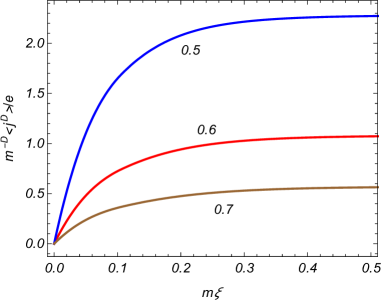
Figure 1: The current density along the compact dimension in the $D=4$ model as a function of $m\xi$. The graphs are plotted for $\tilde{\alpha}_{D}/2\pi=0.2$ and the numbers near the curves correspond to the values of $mL$.

In Figure 2 we have plotted the difference in the current densities for the FR and Minkowski vacua (in units of $em^{D}$) versus the parameter $\tilde{\alpha}_{D}/2\pi$ (left panel) and the length of the compact dimension (right panel) in the model with $D=4$ for a single compact dimension. The numbers near the curves are the values for $m\xi$. On the left panel, for the length of the compact dimension we have taken the value corresponding to $mL=0.5$. The current density is a periodic function of $\tilde{\alpha}_{D}/2\pi$ with the period 1 and the graphs are plotted for a single period. We recall that $\tilde{\alpha}_{D}/2\pi$ is expressed in terms of the magnetic flux threading the compact dimension in units of the flux quantum. The graphs on the right panel are plotted for $\tilde{\alpha}_{D}/2\pi=0.2$. As it has been shown by asymptotic analysis, for $L\ll\xi$ the difference $\langle j^{D}\rangle-\langle j^{D}\rangle_{\mathrm{M}}$ is suppressed by the factor $e^{-2|\tilde{\alpha}_{D}|\xi/L}$ and that is confirmed by the numerical data on the right panel.

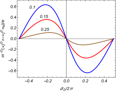
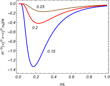
Figure 2: The dependence of the difference of the current densities in the FR and Minkowski vacua on the parameter $\tilde{\alpha}_{D}/2\pi$ (left panel) and on the length of the compact dimension (right panel). The left and right panels are plotted for $mL=0.5$ and $\tilde{\alpha}_{D}/2\pi=0.2$, respectively, and the numbers near the curves correspond to the values of $m\xi$.

4.3 Near-horizon and large-distance vacuum currents around cylindrical black holes

The cylindrical black holes are axially symmetric solutions of the Einstein equations with negative cosmological constant (see, for example, [22]-[28] and references therein). They have also been studied in the context of cosmic strings, supergravity and low energy string theories. The line element for the exterior geometry of a non-rotating and uncharged cylindrical black hole in $(D+1)$-dimensional spacetime has the form (the generalization for rotating and charged black holes can be found in [27])

$$ds_{\mathrm{bh}}^{2}=f(r)dt^{2}-\frac{dr^{2}}{f(r)}-r^{2}\sum_{i=1}^{p}\left(dy^{i}\right)^{2}-r^{2}\sum_{i=1}^{q}\left(d\phi_{i}\right)^{2},$$ (44)

where $p+q+1=D$, $0\leq\phi_{i}<2\pi$, $-\infty<y^{i}<+\infty$, and

$$f(r)=\frac{r^{2}}{a^{2}}-\frac{M}{r^{D-2}}.$$ (45)

The parameters $a$ and $M$ are expressed in terms of negative cosmological constant $\Lambda$ and mass $\mathcal{M}$ per unit volume of the subspace $(y_{1},\ldots,y_{p})$ as

$$a=\sqrt{D\frac{1-D}{2\Lambda}},\;M=\frac{16\pi G_{D+1}}{D-1}\mathcal{M},$$ (46)

where $G_{D+1}$ is the Newton gravitational constant in $(D+1)$-dimensional spacetime. The gravitational field is characterized by two length scales: $a$ and $r_{G}=M^{1/(D-2)}$. For the event horizon one has $r=r_{H}$ with $r_{H}=\left(a^{2}M\right)^{1/D}=r_{G}(a/r_{G})^{2/D}$. In the special case of a $D=3$ cylindrical black hole one has $p=q=1$. For $(2+1)$-dimensional black holes $p=0$ and $q=1$. Some approximate and numerical results for the VEVs of the field squared and energy-momentum tensor for a massless real scalar field in the geometry of 4-dimensional cylindrical black hole were presented in [36, 37].

In Appendix B we show that in the near-horizon limit the line element (44) takes a locally Rindler form (1) with the lengths of the compact dimensions determined by the radius of the horizon $r_{H}$: $L_{l}=2\pi r_{H}$ for $l=p+2,\ldots,D$. From here we conclude that near the horizon the current density along the direction $\phi_{i}$ is expressed by the formulas (25) or (31) with $l=i+p+1$ and

$$\xi=\frac{2a}{\sqrt{D}}\sqrt{r/r_{H}-1}.$$ (47)

Note that these formulas give the physical components. The contravariant components in the coordinate system $(t,r,y_{1},\ldots,y_{p},\phi_{1},\ldots,\phi_{q})$ contain an additional factor $1/r$ that should be replaced by $1/r_{H}$ in the near-horizon limit. From the analysis presented in Appendix B it follows that the expressions (25) or (31) approximate the near-horizon currents for cylindrical black holes under the condition $\left(\xi/a\right)^{2}\ll 1$. For the ratio $\xi/L_{l}$ with $L_{l}=2\pi r_{H}$ one gets $\xi/L_{l}\ll\left(a/r_{G}\right)^{1-2/D}/(2\pi)$. If the length scales $a$ and $r_{G}$ have the same order of magnitude we have $\xi/L_{l}\ll 1$ and the corresponding asymptotics of the formulas (25) or (31) can be used to estimate the current density. In the case $a\gg r_{G}$ the ratio $\xi/L_{l}$ can be of the order of 1 and the exact expressions should be used.

Now let us consider the asymptotic geometry at large distances from the horizon, $r\gg r_{H}$. Expanding the metric tensor and introducing a new coordinate $z=a^{2}/r$, the line element is expressed as

$$ds_{\mathrm{bh}}^{2}\approx\frac{a^{2}}{z^{2}}\left[dt^{2}-dz^{2}-a^{2}\sum_{i=1}^{p}\left(dy^{i}\right)^{2}-a^{2}\sum_{i=1}^{q}\left(d\phi_{i}\right)^{2}\right].$$ (48)

With the new rescaled coordinates $x^{i+1}=ay^{i}$, $i=1,\ldots,p$, and $x^{p+i+1}=a\phi_{i}$, $i=1,\ldots,q$, it attains the form

$$ds_{\mathrm{bh}}^{2}\approx\frac{a^{2}}{z^{2}}\left[dt^{2}-dz^{2}-\sum_{i=2}^{D}\left(dx^{i}\right)^{2}\right],$$ (49)

with $-\infty<x^{i}<+\infty$ for $i=2,\ldots,p+1$, and $0\leq x^{i}\leq 2\pi a$ for $i=p+2,\ldots,D$. The expression in the right-hand side of (49) describes a locally AdS spacetime a part of the coordinates for which are compactified to a torus. The values $z=0$ and $z=\infty$ for the $z$-coordinate correspond to the AdS boundary and horizon, respectively. From the condition $r\gg r_{H}$ it follows that the line element in (49) describes the large-distance asymptotic for cylindrical black holes under the condition $z/a\ll(a/r_{G})^{1-2/D}$. For $a$ and $r_{G}$ having the same order of magnitude this corresponds to points near the AdS boundary.

The VEV of the current density for a scalar field in the geometry described by the right-hand side of (49) with general values $L_{l}$ of the lengths of compact dimensions has been investigated in [38]. In the special case under consideration with $L_{l}=2\pi a$ it is given by the expression

$$\langle j^{l}\rangle\approx\frac{2ea^{-D}}{(2\pi)^{(D-1)/2}}\sum_{\mathbf{n}_{q}}n_{l}\sin\left(\mathbf{n}_{q}\cdot\boldsymbol{\tilde{\alpha}}\right)q_{\nu-1/2}^{(D+1)/2}(1+2\left(\pi r/a\right)^{2}\sum_{i=p+2}^{D}n_{i}^{2}),$$ (50)

where $\nu=\sqrt{D^{2}/4-D(D+1)\zeta+m^{2}a^{2}}$ and $q_{\alpha}^{\mu}(x)=(x^{2}-1)^{-\mu/2}e^{-i\pi\mu}Q_{\alpha}^{\mu}(x)$. Here, $\zeta$ is the curvature coupling parameter and $Q_{\alpha}^{\mu}(x)$ is the associated Legendre function of the second kind [30]. From $r\gg r_{H}$ we get the constraint on the ratio $r/a$ in (50): $r/a\gg\left(r_{G}/a\right)^{1-2/D}$. If the length scales $r_{G}$ and $a$ are of the same order of magnitude, one has $r/a\gg 1$ and, by using the large argument asymptotic for the function $q_{\alpha}^{\mu}(x)$, from (50) we get

$$\langle j^{l}\rangle\approx\frac{4ea^{-D}\Gamma\left(\nu+D/2+1\right)}{\pi^{D/2-1}\Gamma\left(\nu+1\right)\left(2\pi r/a\right)^{D+2\nu+2}}\sideset{}{{}^{\prime}}{\sum}_{\mathbf{n}_{q}}\frac{n_{l}\sin\left(\mathbf{n}_{q}\cdot\boldsymbol{\tilde{\alpha}}\right)}{(n_{p+2}^{2}+\cdots+n_{D}^{2})^{\frac{D}{2}+\nu+1}},$$ (51)

where the prime on the summation sign means that the term with $n_{p+2}=\cdots=n_{D}=0$ should be excluded. For $r_{G}\ll a$ the ratio $r/a$ can be of the order of one and more general expression (50) has to be used.

The influence of branes on the vacuum current density for a charged scalar field in locally AdS spacetime with a toroidal subspace has been investigated in [39, 40]. Branes parallel to the AdS boundary have been considered and the corresponding formulas approximate the large-distance asymptotic for the current density around a cylindrical black hole in the presence of additional boundaries with $r=\mathrm{const}$ (spherical branes).

5 Conclusion

We have investigated the vacuum currents for a charged scalar field in Rindler spacetime with a toroidally compact subspace. It is assumed that the field is prepared in the FR vacuum state and obeys quasi-periodicity condition (5) along $l$th compact dimension. For an external gauge field $A_{\mu}$ a simple configuration is considered with constant components in the compact subspace. Those components and the phases in the condition (5) appear in the expressions for the VEVs of physical quantities in the form of combination (8). The latter is interpreted in terms of the magnetic flux threading the compact dimension. The complete set of scalar mode functions realizing the FR vacuum is given by (9). The components of the momentum in the compact subspace are quantized by the periodicity conditions and the corresponding eigenvalues are given by (10). We have started the investigation by evaluating the mode sum for the Hadamard function. The latter is presented in the form (23), where $G_{\mathrm{M}}(x,x^{\prime})$ is the corresponding function for the Minkowski vacuum in flat spacetime with spatial topology $R^{p+1}\times(S^{1})^{q}$ and the last term describes the difference in the correlations of the vacuum fluctuations in the FR and Minkowski vacua.

The VEV of the current density is obtained from the Hadamard function by using the formula (24). The charge and current densities along uncompact dimensions vanish. The current density along the $l$th compact dimension is presented in two equivalent forms, given by (25) and (31). In both the representations the corresponding current density in the Minkowski vacuum is explicitly extracted. The latter is investigated in the literature and the corresponding VEV is expressed as (26) or, equivalently, by (27). The projection of the current density on $l$th compact dimension is an odd periodic function of the parameter $\tilde{\alpha}_{l}$ and an even periodic function of the parameters $\tilde{\alpha}_{i}$, $i\neq l$, with period $2\pi$. In terms of the magnetic flux enclosed by compact dimensions, this corresponds to periodicity with period equal to the flux quantum. We have shown that the current density vanishes on the Rindler horizon that corresponds to the limit $\xi\rightarrow 0$. The large values of $\xi$ correspond to small accelerations and the difference in the current densities for the FR and Minkowski vacua is exponentially small (see (41)). For small values of the length of compact dimension the difference of the current densities between the FR and Minkowski vacua is exponentially suppressed and the separate current densities along the $l$th compact dimension behave like $1/L_{l}^{D}$. For large values of $L_{l}$ and for $m=0$, $\tilde{\alpha}_{i}=0$, $i\neq l$, one has power-law decay of the Minkowskian contribution, $\langle j^{l}\rangle_{\mathrm{M}}\propto 1/L_{l}^{p+1}$. For $\omega_{0l}\neq 0$ the large $L_{l}$ asymptotic of the VEV $\langle j^{l}\rangle_{\mathrm{M}}$ contains an exponential factor $e^{-L_{l}\omega_{0l}}$ and it falls off more rapidly. In the large $L_{l}$ limit the decay of the difference $\langle j^{l}\rangle-\langle j^{l}\rangle_{\mathrm{M}}$ is stronger than that for $\langle j^{l}\rangle_{\mathrm{M}}$.

As an application of the obtained results we have considered the near-horizon vacuum currents around cylindrical black holes. The corresponding exterior geometry is described by the line element (44). Near the horizon it is approximated by the Rindler-like metric (1) considered in Section 2 with the lengths of the compact dimensions $L_{l}=2\pi r_{H}$ for all $l=p+2,\ldots,D$. At large distances from the horizon the geometry of cylindrical black holes is approximated by a locally AdS spacetime with a toroidally compact subspace. The lengths of the corresponding compact dimensions are expressed in terms of the AdS curvature scale $a$ as $L_{l}=2\pi a$. Similar to the near-horizon approximation, all the compact dimensions have the same length. The vacuum currents in that geometry have been investigated in [38] and are given by the right-hand side of (50).

In the discussion above, as a local characteristic of the FR vacuum state the expectation value of the current density is considered. By using the Hadamard function (23), we can investigate the expectation values for other physical characteristics bilinear in the field operator. Among those characteristics, an important quantity is the VEV of the energy-momentum tensor and the corresponding results for the FR vacuum will be presented elsewhere. Here we mention that the influence of nontrivial spatial topology on the energy of the Minkowski vacuum has been widely considered in the literature for scalar, fermionic and vector fields (see, for example, [32],[42]-[47] and references therein).

Appendix A Representation for the Minkowskian Hadamard function

In this section we provide a representation for the Minkowskian Hadamard function that is convenient in order to compare the topological effects in Minkowski and Rindler spacetimes with compact dimensions. We consider a locally Minkowskian spacetime with the line element (3), where the subspace $(x^{2},x^{3},\ldots,x^{D})$ has the topology $R^{p}\times S^{q}$. By using the corresponding mode sum formula and the Minkowskian eigenfunctions it can be seen that the Minkowskian Hadamard function may be presented in the form

$$G_{\mathrm{M}}(x,x^{\prime})=\frac{2^{-p}}{\pi^{p+1}V_{q}}\int d\mathbf{k}_{p}\sum_{\mathbf{n}_{q}}e^{i\mathbf{k}\cdot\Delta{\mathbf{x}}}K_{0}\left(\lambda_{\mathbf{k}}\sqrt{\xi^{2}+\xi^{\prime 2}-2\xi\xi^{\prime}\cosh\Delta\tau}\right),$$ (52)

where $\xi^{2}+\xi^{\prime 2}-2\xi\xi^{\prime}\cosh\Delta\tau=(x_{\mathrm{M}}^{1}-x_{\mathrm{M}}^{\prime 1})^{2}-(t_{\mathrm{M}}-t_{\mathrm{M}}^{\prime})^{2}$. For the further transformation we use the integral representation [41]

$$K_{0}\left(\lambda\sqrt{\xi^{2}+\xi^{\prime 2}+2\xi\xi^{\prime}\cos b}\right)=\frac{2}{\pi}\int_{0}^{\infty}d\omega\,\cosh(b\omega)K_{i\omega}(\lambda\xi)K_{i\omega}(\lambda\xi^{\prime}),$$ (53)

Taking $b=\pi\pm i\Delta\tau$ we get

$$K_{0}\left(\lambda\sqrt{\xi^{2}+\xi^{\prime 2}+2\xi\xi^{\prime}\cos\left(\pi\pm i\Delta\tau\right)}\right)=\frac{2}{\pi}\int_{0}^{\infty}d\omega\,\cosh\left[\left(\pi\pm i\Delta\tau\right)\omega\right]K_{i\omega}(\lambda\xi)K_{i\omega}(\lambda\xi^{\prime}).$$ (54)

From here it follows that

$$K_{0}\left(\lambda\sqrt{\xi^{2}+\xi^{\prime 2}-2\xi\xi^{\prime}\cosh\Delta\tau}\right)=\frac{2}{\pi}\int_{0}^{\infty}d\omega\,\cosh\left(\pi\omega\right)\cos\left(\omega\Delta\tau\right)K_{i\omega}(\lambda\xi)K_{i\omega}(\lambda\xi^{\prime}).$$ (55)

Combining this relation with (52), the Minkowskian Hadamard function is presented in the form (20).

Appendix B Rindler spacetime with compact dimensions as a near-horizon geometry for cylindrical black holes

In this section we consider the near-horizon limit of the exterior geometry for a cylindrical black hole given by (44). We write $r=r_{H}\left(1+x/D\right)$ and expand the metric for small $x$. To the leading order one gets $f(r)\approx Mx/r_{H}^{D-2}$ and

$$ds_{\mathrm{bh}}^{2}\approx\frac{Mx}{r_{H}^{D-2}}dt^{2}-\frac{a^{2}dx^{2}}{D^{2}x}-r_{H}^{2}\sum_{i=1}^{p}\left(dy^{i}\right)^{2}-r_{H}^{2}\sum_{i=1}^{q}\left(d\phi_{i}\right)^{2}.$$ (56)

Introducing the coordinate $\xi$ in accordance with $x=\left(D\xi/2a\right)^{2}$, the line element is rewritten as

$$ds_{\mathrm{bh}}^{2}\approx\frac{D^{2}M}{4a^{2}r_{H}^{D-2}}\xi^{2}dt^{2}-d\xi^{2}-r_{H}^{2}\sum_{i=1}^{p}\left(dy^{i}\right)^{2}-r_{H}^{2}\sum_{i=1}^{q}\left(d\phi_{i}\right)^{2}.$$ (57)

In terms of the new coordinates

$$\tau=\frac{D\sqrt{M}}{2ar_{H}^{D/2-1}}t,\;x^{i+1}=r_{H}y^{i},\;x^{p+l+1}=r_{H}\phi_{l},$$ (58)

with $i=1,\ldots,p$, $l=1,\ldots,q$, this line element attains a locally Rindler form

$$ds_{\mathrm{bh}}^{2}\approx\xi^{2}d\tau^{2}-d\xi^{2}-\sum_{i=2}^{D}\left(dx^{i}\right)^{2},$$ (59)

where $-\infty<x^{i}<+\infty$ for $i=2,\ldots,p+1$, and $0\leq x^{i}\leq 2\pi r_{H}$ for $i=p+2,\ldots,D$.

References

• [1] N. D. Birrell and P. C. W. Davies, Quantum Fields in Curved Space (Cambridge University Press, Cambridge, 1982).
• [2] S. A. Fulling, Nonuniqueness of canonical field quantization in Riemannian space-time. Phys. Rev. D 7, 2850 (1973).
• [3] R. Emparan, AdS/CFT duals of topological black holes and the entropy of zero-energy states. J. Hihg Energy Phys. 06(1999)036.
• [4] A. Hamilton, D.N. Kabat, G. Lifschytz, and D.A. Lowe, Holographic representation of local bulk operators. Phys. Rev. D 74, 066009 (2006).
• [5] M. Parikh, P. Samantray, and E. Verlinde, Rotating Rindler-AdS space. Phys. Rev. D 86, 024005 (2012).
• [6] B. Czech, J. L. Karczmarek, F. Nogueira, and M. Van Raamsdonk, Rindler quantum gravity. Class. Quant. Grav. 29, 235025 (2012).
• [7] P. Samantray and T. Padmanabhan, Conformal symmetry, Rindler space, and the AdS/CFT correspondence. Phys. Rev. D 90, 047502 (2014).
• [8] M. Parikh and P. Samantray, Rindler-AdS/CFT. J. Hihg Energy Phys. 10(2018)129.
• [9] V. M. Mostepanenko and N. N. Trunov, The Casimir Effect and Its Applications (Clarendon,Oxford, 1997).
• [10] K. A. Milton, The Casimir Effect: Physical Manifestation of Zero-Point Energy (World Scientific, Singapore, 2002).
• [11] M. Bordag, G. L. Klimchitskaya, U. Mohideen, and V. M. Mostepanenko, Advances in the Casimir Effect (Oxford University Press, New York, 2009).
• [12] Casimir Physics, edited by D. Dalvit, P. Milonni, D. Roberts, and F. da Rosa, Lecture Notes in Physics Vol. 834 (Springer-Verlag, Berlin, 2011).
• [13] P. Candelas and D. Deutsch, Proc. R. Soc. London A 354, 79 (1977).
• [14] A. A. Saharian, Polarization of the Fulling-Rindler vacuum by a uniformly accelerated mirror. Class. Quantum Grav. 19, 5039 (2002).
• [15] R. M. Avagyan, A. A. Saharian, and A. H. Yeranyan, Casimir effect in the Fulling-Rindler vacuum. Phys. Rev. D 66, 085023 (2002).
• [16] A. A. Saharian, R. S. Davtyan, and A. H. Yeranyan, Casimir energy in the Fulling-Rindler vacuum. Phys. Rev. D 69, 085002 (2004).
• [17] A. A. Saharian and M. R. Setare, Surface vacuum energy and stresses on a plate uniformly accelerated through the Fulling-Rindler vacuum. Class. Quantum Grav. 21, 5261 (2004).
• [18] A. A. Saharian and M. R. Setare, Casimir energy-momentum tensor for a brane in de Sitter spacetime. Phys. Lett. B 584, 306 (2004).
• [19] A. A. Saharian, R. M. Avagyan, and R. S. Davtyan, Wightman function and Casimir densities for Robin plates in the Fulling-Rindler vacuum. Int. J. Mod. Phys. A 21, 2353 (2006).
• [20] A. A. Saharian and M. R. Setare, Casimir densities for a spherical brane in Rindler-like spacetimes. Nucl. Phys. B 724, 406 (2005).
• [21] A. A. Saharian and M. R. Setare, Surface Casimir densities on a spherical brane in Rindler-like spacetimes Phys. Lett. B 637, 5 (2006).
• [22] J. P. S. Lemos, Cylindrical black hole in general relativity. Phys. Lett. B 353, 46 (1995).
• [23] J. P. S. Lemos and V. T. Zanchin, Rotating charged black strings and three-dimensional black holes. Phys. Rev. D 54, 3840 (1996).
• [24] R.-G. Cai and Y.-Z. Zhang, Black plane solutions in four-dimensional spacetimes. Phys. Rev. D 54, 4891 (1996).
• [25] G. T. Horowitz and R. C. Myers, AdS-CFT correspondence and a new positive energy conjecture for general relativity. Phys. Rev. D 59, 026005 (1998).
• [26] C. Martinez, C. Teitelboim, and J. Zanelli, Charged rotating black hole in three space-time dimensions. Phys. Rev. D 61, 104013 (2000).
• [27] A. M. Awad, Higher dimensional charged rotating solutions in (A)dS space-times. Class. Quant. Grav. 20, 2827 (2003).
• [28] M. B. Gaete, L. Guajardo, and M. Hassaïne, A Cardy-like formula for rotating black holes with planar horizon. J. Hihg Energy Phys. 04(2017)092.
• [29] L. C. B. Crispino, A. Higuchi, and G. E. A. Matsas, The Unruh effect and its applications. Rev. Mod. Phys. 80, 787 (2008).
• [30] Handbook of Mathematical Functions, edited by M. Abramowitz, I. A. Stegun (Dover, New York, 1972).
• [31] P. Candelas and D. J. Raine, Quantum field theory on incomplete manifolds. J. Math. Phys. 17, 2101 (1976).
• [32] F. C. Khanna, A. P. C. Malbouisson, J. M. C. Malbouisson, and A. E. Santana, Quantum field theory on toroidal topology: Algebraic structure and applications. Phys. Rep. 539, 135 (2014).
• [33] K. Rajeev and T. Padmanabhan, Exploring the Rindler vacuum and the Euclidean plane. J. Math. Phys. 61, 062302 (2020).
• [34] G. N. Watson, A Treatise on the Theory of Bessel Functions (Cambridge University Press, Cambridge, England, 1966).
• [35] E. R. Bezerra de Mello and A. A. Saharian, Finite temperature current densities and Bose-Einstein condensation in topologically nontrivial spaces. Phys. Rev. D 87, 045015 (2013).
• [36] A. DeBenedictis, Gravitational effects of quantum fields in the interior of a cylindrical black hole. Class. Quantum Grav. 16, 1955 (1999).
• [37] A. DeBenedictis, $\langle\phi^{2}\rangle$ in the spacetime of a cylindrical black hole. Gen. Rel. Grav. 32, 1549 (1999).
• [38] E. R. Bezerra de Mello, A. A. Saharian, and V. Vardanyan, Induced vacuum currents in anti-de Sitter space with toral dimensions. Phys. Lett. B 741, 155 (2015).
• [39] S. Bellucci, A. A. Saharian, and V. Vardanyan, Vacuum currents in braneworlds on AdS bulk with compact dimensions. J. Hihg Energy Phys. 11(2015)092.
• [40] S. Bellucci, A. A. Saharian, and V. Vardanyan, Hadamard function and the vacuum currents in braneworlds with compact dimensions: Two-brane geometry. Phys. Rev. D 93, 084011 (2016).
• [41] A. P. Prudnikov, Yu. A. Brychkov, and O. I. Marichev, Integrals and Series (Gordon and Breach, New York, 1986), Vol. 2.
• [42] A. Edery and V. N. Marachevsky, Compact dimensions and the Casimir effect: the Proca connection. J. High Energy Phys. 12(2008)035.
• [43] E. Elizalde, S. D. Odintsov, and A. A. Saharian, Repulsive Casimir effect from extra dimensions and Robin boundary conditions: From branes to pistons. Phys. Rev. D 79, 065023 (2009).
• [44] S. Bellucci1 and A. A. Saharian, Fermionic Casimir densities in toroidally compactified spacetimes with applications to nanotubes. Phys. Rev. D 79, 085019 (2009).
• [45] L. P. Teo, Electromagnetic Casimir piston in higher-dimensional spacetimes. Phys. Rev. D 83, 105020 (2011).
• [46] C. J. Cao, M. van Caspel, and A. R. Zhitnitsky, Topological Casimir effect in Maxwell electrodynamics on a compact manifold. Phys. Rev. D 87, 105012 (2013).
• [47] S. R. Haridev and P. Samantray, Revisiting vacuum energy in compact spacetimes. arXiv:2106.12171.