Phenomenological theory of magnetic 90^∘ helical state

Abstract

We explore a phenomenological phase diagram for the magnetic helical state with 90^∘ turn angle between neighboring spins in the external magnetic field. Such state is formed by the Eu spin layers in the superconducting iron arsenide RbEuFe₄As₄. The peculiarity of this spin configuration is that it is not realized in the standard Heisenberg model with bilinear exchange interactions. A minimum model allowing for such a state requires the biquadratic nearest-neighbor interaction term. In addition, in tetragonal materials the 90^∘ helix state may be stabilized by the in-plane four-fold anisotropy term, which also fixes helix orientation with respect to the crystal lattice. Such a system has a very rich behavior in the external magnetic field. The magnetic field induces the metamagnetic transition to the double-periodic state with the moment angles ($\alpha$, $\alpha$, $-\alpha$, $-\alpha$) with respect to the field for the four subsequent spins. The transition field to this state from the deformed helix is determined by the strength of biquadratic interaction. The transition is second order for small biquadratic coupling and becomes first order when this coupling exceeds the critical value. On the other hand, the aligned state at high magnetic field becomes unstable with respect to formation of incommensurate fan state which transforms into the double-periodic state with decreasing magnetic field. The range of this incommensurate state near the saturation field is proportional to square of the biquadratic coupling. In addition, when the magnetic field is applied along one of four the equilibrium moment directions, the deformed helix state experience the first-order rotation transition at the field determined by the four-fold anisotropy.

I Introduction

Several magnetic materials have noncollinear helical ground states, in which spins ferromagnetically align within layers but rotate from layer to layer at a finite angle around the helix axis. In materials without inversion symmetry, such as MnSi[1], FeGe[2], and Fe${}_{1\text{\textendash}x}$Co_xSi[3, 4], these helical configurations are caused by Dzyaloshinskii-Moriya interaction and, due to the weakness of this interaction, the structure period is very large. Helical states are also realized in materials with inversion symmetry, such as EuNi₂As₂[5, 6] and EuCo₂P₂[7, 8]. In this case, they emerge due to competing exchange interactions[9, 10, 11, 12]. The simplest case is the next-nearest neighbor classical Heisenberg model described by the energy functional

$$E\! =\!-\sum_{n}\left(J_{z,1}\boldsymbol{s}_{n}\boldsymbol{s}_{n+1}\!+\!J_{z,2}\boldsymbol{s}_{n}\boldsymbol{s}_{n+2}\right)$$ (1)

$$=\!-\sum_{n}\left[J_{z,1}\cos\left(\phi_{n+1}\!-\!\phi_{n}\right)\!+\!J_{z,2}\cos\left(\phi_{n+2}\!-\!\phi_{n}\right)\right],$$

where $\boldsymbol{s}_{n}\!=\!\left(\cos\phi_{n},\sin\phi_{n},0\right)$ is the unit in-plane vector along the spin direction in n^th layer. For this model, the ground helical state $\phi_{n}^{(0)}=Qn$ is realized for the relation between the exchange constants $J_{z,2}\!<\!-|J_{z,1}|/4$ with $\cos Q\!=\!-J_{z,1}/(4J_{z,2})$ [9, 10, 11, 12]. In metallic magnets, the frustration may be caused by the oscillating interaction between spins mediated by conduction electrons, known as Ruderman-Kittel-Kasuya-Yosida (RKKY) interaction. A special case of helical magnetism is predicted in superconducting ferromagnets [13, 14, 15, 16], where the origin of frustration is the competition between the normal and superconducting RKKY interactions. Experimentally, a helical magnetic state has been established in the nickel borocarbide HoNi₂B₂C[17, 18]. Such state may also realize in superconducting compound ErRh₄B₄[13, 19].

Recently, the helical magnetic state has been found in the superconducting iron pnictide RbEuFe₄As₄ [20, 21]. In this state, the Eu moments align ferromagnetically in Eu layers and rotate 90^∘ from layer to layer. Such 90^∘ helix state is unique, because it does not exist within the above simple Heisenberg exchange model [11] and its stabilization requires spin interactions beyond common bilinear terms. Indeed, in the above framework, formally, the 90^∘ helix, $Q\!=\!\pi/2$, is supposed to realize when the nearest-neighbor constant vanishes, $J_{z,1}\!=\!0$, and the next-nearest-neighbor constant is negative, $J_{z,2}<0$. However, in this case, the interaction between two sublattices composed of odd and even spin layers is absent so that the energy is degenerate with respect to relative rotation of these sublattices[22, 12]. The 90^∘ helix is only one of such states corresponding to the orthogonal orientation of the sublattices moments. Adding interactions with more remote layers does not resolve this issue. Therefore, the stabilization of the 90^∘ helical state requires inclusions of nonconventional spin interactions. The simplest such interaction is the nearest-neighbor biquadratic term $J_{z,b}\left(\boldsymbol{s}_{n}\boldsymbol{s}_{n+1}\right)^{2}$. It breaks rotational degeneracy between two sublattices and, when the interaction constant is positive, $J_{z,b}>0$, favors 90^∘ helix.

Biquadratic spin interactions between local magnetic moments were considered before in different situations. Such interaction was first introduced in Ref. [23] to describe the interaction between Mn²⁺ moments inside MgO crystal. Later, the presence of the biquadratic interaction has been experimentally established in the Fe-Cr-Fe sandwiches [24, 25]. In particular, for certain thicknesses of interlayer Cr, this interaction leads to the perpendicular orientation of the magnetization in two Fe films. After this discovery, the presence of the biquadratic interaction has been demonstrated in many other sandwich structures, see review [25] and references therein. More recently, the biquadratic term was introduced to explain unusual ’up-up-down-down’ magnetic structure in several manganites, such as HoMnO₃[26]. Contrary to 90^∘ helix, such double-periodic state is realized for negative $J_{z,b}$. The most straightforward intrinsic origin of the biquadratic coupling between magnetic moments in metallic systems is the higher-order expansion terms of the energy with respect to the exchange interaction between the moments and conduction electrons, see, e.g., Refs. [27, 28]. Other mechanisms for this coupling were also theoretically proposed for different physical systems [26, 29, 30].

Biquadratic interactions are also likely are relevant for the magnetic properties of iron pnictides. For example, the biquadratic coupling between the Fe spins has to be taken into account to explain the domain-wall structure and the spin-wave spectrum in the stripe antiferromagnetic state in FeAs layers[31]. The biquadratic coupling between Eu and Fe spins in EuFe₂As₂ has been also introduced in Ref. [32, 33] to model magnetic detwinning. Therefore, the assumption of a noticeable biquadratic interaction between Eu spin layers in RbEuFe₄As₄ does not look too exotic. The vanishing of nearest-neighbor exchange in this material may be the result of an accidental compensation of the normal and superconducting contributions to the RKKY interaction [34]. The biquadratic term is most likely caused by the interaction between spins mediated by superconducting electrons.

In the model with only bilinear and biquadratic exchange interactions, the energy is degenerate with respect to helix rotation. This continuous degeneracy is eliminated by the 4-fold crystal anisotropy term, $-K_{4}(s_{x,\boldsymbol{i},n}^{4}+s_{y,\boldsymbol{i},n}^{4})$. In addition, such anisotropy term locks $Q\!=\!\pi/2$ state within a finite range of the small next-neighbor exchange constant $J_{z,1}$, see Appendix A. Nevertheless, since the 90^∘ helix only exists if $J_{z,1}$ is small, for simplicity, we assume that $J_{z,1}\!=\!0$ in the main text. Therefore, the 90^∘ helical state in the magnetic field applied perpendicular to the helix axis can be described by the following energy functional

$$\mathcal{E} =\sum_{n}\left[|J_{z,2}|\boldsymbol{s}_{n}\boldsymbol{s}_{n+2}+J_{z,b}\left(\boldsymbol{s}_{n}\boldsymbol{s}_{n+1}\right)^{2}+K_{4}\left(s_{x,n}^{4}+s_{y,n}^{4}-\frac{3}{4}\right)-\mu\boldsymbol{H}\boldsymbol{s}_{n}\right]$$

$$=\! \sum_{n}\left[|J_{z,2}|\cos\left(\phi_{n+2}\!-\!\phi_{n}\right)\!+\!J_{z,b}\cos^{2}\left(\phi_{n+1}\!-\!\phi_{n}\right)\!+\!\frac{K_{4}}{4}\cos(4\phi_{n})\!-\!\mu H\cos\left(\phi_{n}\!-\!\theta\right)\right],$$ (2)

where $\mu=g\mu_{B}S$ is the magnetic moment, $S$ is the spin, and $\theta$ is the in-plane angle of the external magnetic field $\boldsymbol{H}\!=\!H(\cos\theta,\sin\theta,0)$. At zero field the ground state of this model is given by the 90^∘ helix with one of the spins oriented at 45^∘ with respect to the $x$ axis. As other spirals, the ground state is chiral and degenerate with respect to the direction of rotation, i.e., the spiral can be either right hand or left hand.

The goal of this paper is to investigate the magnetic phase diagram following from the energy functional in Eq. (2). The overall behavior for this model is fully determined by the two dimensionless parameters, $r_{b}=J_{z,b}/|J_{z,2}|$ and $k_{4}\equiv K_{4}/|J_{z,2}|$, both of which are expected to be small. We also introduce the reduced magnetic field $\tilde{h}=\mu H/|J_{z,2}|$. The equilibrium spin angles $\phi_{n}$ determine the magnetization per spin, $m=\left\langle\cos\phi_{n}\right\rangle$. In real units it determines the bulk magnetization normalized to its saturation value, $m=M/M_{\mathrm{sat}}$, with $M_{\mathrm{sat}}=\mu n_{M}$, where $n_{M}$ is the bulk density of the moments.

A detailed investigation of helical magnetic structures with different commensurate modulation wave vectors $Q$ within the Heisenberg model in Eq. (1) has been performed in Ref. [12]. A small magnetic field applied perpendicular to the helix axis distorts the helix. With further increase of the field, the distorted helix transforms into the fanlike structure with $\phi_{n}=\phi_{\mathrm{max}}\sin[(n+\alpha)Q]$ first proposed in Ref. [9]. The nature of this transformation is determined by the modulation wave vectors $Q$ and several different scenarios may be realized[12]. For long-wave structures with $Q<4\pi/9$, the first-order transition takes place at a certain transition field $H_{t}$, at which the magnetization jumps. In the range $4\pi/9<Q<\pi$ the behavior is not universal. Typically, the transformation occurs as a smooth crossover but at several commensurate values of $Q$ either first- or second-order phase transitions take place. The fan state exists until the magnetic field reaches the saturation field, at which the fan angle $\phi_{\mathrm{max}}$ vanishes.

We will see that the phase diagram of 90^∘ helix following from Eq. (2) is very rich and has both similarities with and differences from other magnetic spiral structures. The main findings of this paper can be summarized as follows. (i)Small magnetic field distorts the helix and induces phase transition into the double-periodic state, in which the four subsequent spins form the angles ($\alpha$, $\alpha$, $-\alpha$, $-\alpha$) with respect to the field. This state is actually a particular case of a commensurate fan[12]. At small biquadratic coupling this transition is continuous and it becomes first order when the biquadratic coupling exceeds a certain critical value. (ii) The saturated state at high magnetic fields becomes unstable with respect to the incommensurate-fan state with decreasing field. This state occupies the field range proportional to the biquadratic coupling squared and transforms into the double-periodic state when magnetic field decreases below certain level. (iii)For the finite in-plane four-fold anisotropy and the magnetic field applied along one of the four easy-axis directions, there is an additional small-field first-order phase transition corresponding to 45^∘ rotation of the helix.

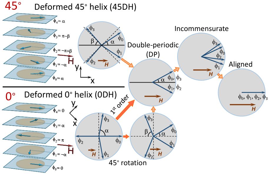
Figure 1: Spin configurations realized with increasing magnetic field for two field orientations for the model with four-fold anisotropy. The upper sequence also describes states for the rotationally-degenerate model with $k_{4}=0$.

The paper is organized as follows. In Sec. II, we investigate the phase diagram of the rotationally-degenerate model with $k_{4}\!=\!0$, which is determined by only one parameter $r_{b}$. We find the transition field to the double-periodic state as a function of this parameter and evaluate the value of $r_{b}$ above which the transition becomes first order. Analyzing the same system at high magnetic fields, we find that the incommensurate-fan state emerges below the saturation field. We evaluate the transition field between this state and the double-periodic state. We also compute the field dependences of the magnetization for different $r_{b}$ and find its features at the transition points. In Sec. III, we study the model with finite four-fold anisotropy which fixes helix orientation and sets four easy-axis directions. We investigate the phase diagrams and the magnetization for the magnetic field applied along the two symmetry directions, along the equilibrium spin orientation and at 45^∘ with respect to this direction. In particular, for the former field orientation, we investigate the first-order helix-rotation transition. Finally, we summarize and discuss the obtained results in Sec. IV.

II Rotationally-degenerate system without four-fold anisotropy

Before the investigation of the full model described by Eq. (2), we consider a simpler model without four-fold anisotropy, $K_{4}=0$, corresponding to a rotationally-degenerate helix. In this case, the magnetic response is controlled by one reduced parameter $r_{b}$. In general, the equilibrium configuration of the spin angles $\phi_{n}$ obeys the equations

$$\sin\left(\phi_{n+2}\!-\!\phi_{n}\right)\!+\!\sin\left(\phi_{n-2}\!-\!\phi_{n}\right)$$

$$+r_{b}\left(\sin\left[2\left(\phi_{n+1}\!-\!\phi_{n}\right)\right]\!+\!\sin\left[2\left(\phi_{n-1}\!-\!\phi_{n}\right)\right]\right)$$

$$+\tilde{h}\sin\left(\phi_{n}\!-\!\theta\right)=\!0.$$ (3)

If we assume that the four-spin periodicity is maintained in the magnetic field, $\phi_{n+4}=\phi_{n}$ then Eq. (3) gives four nonlinear equations for the four phases with $n=0,1,2,3$. Further analysis shows that for small $r_{b}$ the four-spin periodicity is maintained in the most part of the phase diagram but is violated near the saturation field.

The magnetic field breaks down the rotational degeneracy of the helix. In the energy expansion with respect to the magnetic field $\tilde{h}$, the quadratic term is isotropic with respect to the field orientation, while the quartic term, in addition to an isotropic contribution, has also the angle-dependent part proportional to $\tilde{h}^{4}(\cos^{4}\vartheta_{h}\!+\!\sin^{4}\vartheta_{h})$, where $\vartheta_{h}$ is the angle between the field and one of the equilibrium moment directions. The favorable helix orientation is determined by the sign of the coefficient in front of this term. To find this equilibrium helix orientation at a small magnetic field, we compare the energies for two symmetric orientations shown in Fig. 1, which we refer to as deformed 45^∘ helix (45DH) and deformed 0^∘ helix (0DH) shown in the upper and lower 3D picture, respectively. The energy difference between these orientations determines the coefficient in the above angle-dependent quartic term in the energy expansion.

For the 45^∘ helix, the four angles $\phi_{n}$ are determined by only two independent angles $\alpha$ and $\beta$, see the left picture in the upper part of Fig. 1,

$$\phi_{0}=\alpha,\,\phi_{1}=-\alpha,\,\phi_{2}=\pi+\beta,\,\phi_{3}=\pi-\beta,$$ (4)

and at zero field, we have $\alpha\!=\!\beta\!=\!\pi/4$. The reduced energy per spin, $E_{s}=\mathcal{E}_{\mathrm{lay}}/N|J_{z,2}|$, for this state

$$E_{s}\left(\alpha,\beta\right) \!=\!-\cos\left(\beta\!-\!\alpha\right)\!$$

$$+ \frac{r_{b}}{4}\left[\cos^{2}\left(2\alpha\right)\!+\!\cos^{2}\left(2\beta\right)\!+\!2\cos^{2}\left(\beta\!+\!\alpha\right)\right]$$

$$- \frac{\tilde{h}}{2}\left(\cos\alpha-\cos\beta\right)$$ (5)

yields the equations for the equilibrium angles $\alpha$ and $\beta$

$$2\sin\left(\beta\!-\!\alpha\right)\!+\!r_{b}\left(\sin(4\alpha)\!+\!\sin\left[2(\alpha\!+\!\beta)\right]\right)\!-\!\tilde{h}\sin\alpha\!=\!0,\ \ \ \$$ (6a)

$$2\sin\left(\beta\!-\!\alpha\right)\!-\!r_{b}\left(\sin(4\beta)\!+\!\sin\left[2(\alpha\!+\!\beta)\right]\right)\!-\!\tilde{h}\sin\beta\!=\!0.\ \ \ \$$ (6b)

These two angles determine the reduced magnetization per spin,

$$m=\left(\cos\alpha-\cos\beta\right)/2.$$ (7)

Small magnetic field induces small deviations, which we represent as $\alpha\!=\!\frac{\pi}{4}\!-\!\alpha_{+}\!-\frac{\alpha_{-}}{2}$, $\beta\!=\!\frac{\pi}{4}+\!\alpha_{+}\!-\frac{\alpha_{-}}{2}$. Expanding the energy with respect to the small deviations, $\alpha_{\pm}$, we obtain

$$E_{s}\left(\alpha_{+},\alpha_{-}\right) \approx-1+2\left(1+r_{b}\right)\alpha_{+}^{2}+r_{b}\alpha_{-}^{2}$$

$$- \frac{2(1\!+\!4r_{b})}{3}\alpha_{+}^{4}-\frac{r_{b}}{3}\left(12\alpha_{+}^{2}\alpha_{-}^{2}+\alpha_{-}^{4}\right)$$

$$- \frac{\sqrt{2}\tilde{h}}{4}\left(2\alpha_{+}\!-\!\alpha_{+}\alpha_{-}\!-\frac{1}{3}\alpha_{+}^{3}\!-\frac{1}{4}\alpha_{+}\alpha_{-}^{2}\right).$$ (8)

Minimization of this energy gives equations for equilibrium $\alpha_{\pm}$,

$$4\left(1\!+\!r_{b}\right)\alpha_{+}\!-\frac{8(1\!+\!4r_{b})}{3}\alpha_{+}^{3}\!-\!8r_{b}\alpha_{+}\alpha_{-}^{2}\!$$

$$-\frac{\sqrt{2}\tilde{h}}{4}\left(2\!-\!\alpha_{-}\!-\!\alpha_{+}^{2}\!-\!\frac{1}{4}\alpha_{-}^{2}\right)=0,$$ (9a)

$$2r_{b}\alpha_{-}\!-\frac{4r_{b}}{3}\left(6\alpha_{+}^{2}\alpha_{-}\!+\!\alpha_{-}^{3}\right)\!+\frac{\sqrt{2}\tilde{h}}{4}\left(\alpha_{+}\!+\frac{1}{2}\alpha_{+}\alpha_{-}\right)\!=\!0,$$ (9b)

which we expand with respect to $\tilde{h}$

$$\alpha_{\pm}=\sum_{n=1}^{\infty}\alpha_{\pm}^{(n)}\tilde{h}^{n}.$$ (10)

A simple analysis shows that only odd $\alpha_{+}^{(n)}$ and even $\alpha_{-}^{(n)}$ are finite, $\alpha_{+}^{(2k)}=\alpha_{-}^{(2k-1)}=0$. For the expansion coefficients, we derive from Eqs. (9b)

$$\alpha_{+}^{(1)} =\frac{\sqrt{2}}{8\left(1+r_{b}\right)},$$ (11a)

$$\alpha_{-}^{(2)} =-\frac{1}{32r_{b}\left(1+r_{b}\right)},$$ (11b)

$$\alpha_{+}^{(3)} =\frac{\sqrt{2}}{512\left(1\!+\!r_{b}\right)^{4}}\left[\frac{4(1\!+\!4r_{b})}{3}+\!1\!+\frac{1}{r_{b}}\right],$$ (11c)

Substituting the expansion in Eq. (10) with these coefficients into Eq. (8), we finally obtain the energy expansion

$$E_{s}(\tilde{h})\!\approx\!-1\!-\frac{\tilde{h}^{2}}{16\left(1\!+\!r_{b}\right)}-\frac{1\!+\!2r_{b}^{2}/\left(1\!+\!r_{b}\right)^{2}}{1024r_{b}\left(1\!+\!r_{b}\right)^{2}}\tilde{h}^{4}.$$ (12)

From this result, we can also obtain the magnetization at small fields, $m=-dE_{s}/d\tilde{h}$,

$$m(\tilde{h})\approx\frac{\tilde{h}}{8\left(1\!+\!r_{b}\right)}+\frac{1\!+\!2r_{b}^{2}/\left(1\!+\!r_{b}\right)^{2}}{256r_{b}\left(1\!+\!r_{b}\right)^{2}}\tilde{h}^{3}.$$ (13)

It is characterized by the upward curvature which becomes more pronounced at smaller $r_{b}$.

Consider now the deformed 0^∘ helix, see Fig. 1. This state is determined by just one angle $\alpha$ as $\phi_{0}=0$, $\phi_{3}=-\phi_{1}=\alpha$, $\phi_{2}=\pi$, and its energy is

$$E_{s} \!=-1+\left(1+r_{b}\right)\cos^{2}\alpha-\frac{\tilde{h}}{2}\cos\alpha.$$ (14)

Finding its minimum, we obtain

$$\cos\alpha =\frac{\tilde{h}}{4\left(1+r_{b}\right)},$$ (15a)

$$E_{s}(\tilde{h}) =-1-\frac{\tilde{h}^{2}}{16\left(1+r_{b}\right)}.$$ (15b)

Note that the quartic term is absent for this helix orientation. Comparing this result with Eq. (12), we find the quartic angle-dependent term in the energy

$$E_{s}^{(4)}(\vartheta_{h}) =C_{4}\tilde{h}^{4}\left[-1+\cos^{4}\vartheta_{h}\!+\!\sin^{4}\vartheta_{h}\right]$$

$$=-2C_{4}\tilde{h}^{4}\cos^{2}\vartheta_{h}\sin^{2}\vartheta_{h}$$ (16)

$$\text{with }\ C_{4}=\frac{1+2r_{b}^{2}/\left(1+r_{b}\right)^{2}}{512r_{b}\left(1+r_{b}\right)^{2}}$$

We see that the magnetic field breaks down the rotational degeneracy and favors the 45^∘ deformed helix state shown in Fig. 1. From now on, we consider the evolution of this state with increasing magnetic field.

A finite biquadratic coupling favors perpendicular orientation between the moments in odd and even layers. On the other hand, the magnetic field wants to orient the moments in both sublattices in the same way. This means that at small $r_{b}$, one can expect a metamagnetic transition to the double-periodic (DP) state with increasing the magnetic field with $\phi_{3}=\phi_{0}$ and $\phi_{2}=\phi_{1}$, (the state in the middle of Fig. 1). Importantly, a chiral nature of the state vanishes at this transition, since the mirror image can be matched with the original spin configuration. We proceed with the analysis of this double-periodic state and investigation of the transition to it.

II.1 Double-periodic state at high $\tilde{h}$

At high fields the double-periodic state is realized, in which $\beta=\pi-\alpha$, and

$$\phi_{0}=\phi_{3}=\alpha,\,\phi_{1}=\phi_{2}=-\alpha.$$ (17)

Since such angle distribution can also be presented as $\phi_{n}=-\sqrt{2}\alpha\sin\left[(n\!-\!1/2)\pi/2\right]$, this state formally belongs to the family of fanlike states[12]. The energy of this double-periodic state

$$E_{s}\left(\alpha,\pi\!-\!\alpha\right) \!=\!\cos\left(2\alpha\right)\!+\frac{r_{b}}{2}\left[1\!+\!\cos^{2}\left(2\alpha\right)\right]\!-\!\tilde{h}\cos\alpha$$ (18)

gives the equation for the equilibrium angle

$$4\cos\alpha_{0}\left[1+r_{b}\cos\left(2\alpha_{0}\right)\right] =\tilde{h}.$$ (19)

The limit $\alpha_{0}\!=\!0$ formally corresponds to saturation (the right state in Fig. 1). This condition gives the nominal saturation field $\tilde{h}_{\mathrm{sat}}^{\mathrm{DP}}\!=4\left(1\!+\!r_{b}\right)$. We will show in the next section, however, that the double-periodic state transforms into a incommensurate-fan state with increasing magnetic field. As a consequence, the true saturation field is somewhat higher than the above value.

To find the stability range of the double-periodic state, we consider a small deviation from the double periodicity, $\alpha\!=\!\alpha_{0}\!+\!\psi$, $\beta\!=\!\pi\!-\!\alpha_{0}\!+\!\psi$ with $\psi\!\ll\!1$. The energy expansion

$$\delta E_{s}^{(2)}\left(\psi\right) =\left[-4r_{b}\cos^{2}\left(2\alpha_{0}\right)+\frac{\tilde{h}}{2}\cos\alpha_{0}\right]\psi^{2}$$ (20)

obtained from Eq. (5) gives the stability condition

$$-8r_{b}\cos^{2}\left(2\alpha_{0}\right)+\tilde{h}\cos\alpha_{0}>0.$$ (21)

Combining this equation with Eq. (19) for the equilibrium angle, we find $\cos\left(2\alpha_{0}\right)$ at the instability point

$$\cos\left(2\alpha_{0}\right)=-\frac{2}{1\!+\!r_{b}\!+\!\mathcal{R}_{0}}$$ (22)

with $\mathcal{R}_{0}\equiv\sqrt{\left(1\!+\!r_{b}\right)^{2}\!+\!12r_{b}}.$ This gives

$$\cos\alpha_{0}=\frac{\sqrt{r_{b}}\left[r_{b}\!+\!7\!+\!\mathcal{R}_{0}\right]^{1/2}}{1+r_{b}+\mathcal{R}_{0}}.$$ (23)

For $r_{b}\rightarrow 0$, the instability angle approaches $\pi/2$. Eqs. (22) and (23) allow us to obtain the analytic result for the instability field from Eq. (21)

$$\tilde{h}_{i}=\frac{4\sqrt{r_{b}}\left[r_{b}\!+\!7\!+\!\mathcal{R}_{0}\right]^{1/2}\!\left(1\!-\!r_{b}\!+\!\mathcal{R}_{0}\right)}{\left(1+r_{b}+\mathcal{R}_{0}\right)^{2}}.$$ (24)

The double-periodic state is stable for $\tilde{h}>\tilde{h}_{i}$. In the limit $r_{b}\ll 1$, we obtain a simple asymptotics

$$\tilde{h}_{i}\simeq 4\sqrt{2r_{b}},$$ (25)

i. e., at small $r_{b}$ the instability field decrease proportionally to $\sqrt{r_{b}}$ and in this case the double-periodic state occupies a wide range of magnetic fields. In real units the result in Eq. (25) becomes $H_{i}\simeq 4\sqrt{2J_{z,b}|J_{z,2}|}/\mu$.

The instability field in Eq. (24) corresponds to a second-order phase transition only if the coefficient $c_{4}$ in the quartic energy expansion term, $\delta E_{s}^{(4)}=\frac{1}{4}c_{4}\psi^{4}$, is positive. Calculations described in Appendix B give the following result for the quartic coefficient at the instability point,

$$c_{4}(r_{b}) =20r_{b}u^{2}-\frac{\left(1-u^{2}\right)\left(1+15r_{b}u\right)^{2}}{2\left(r_{b}+u\right)},$$ (26)

$$u(r_{b})= -\cos\left(2\alpha_{0}\right)=\frac{2}{1\!+\!r_{b}\!+\!\sqrt{\left(1\!+\!r_{b}\right)^{2}\!+\!12r_{b}}}.$$

The parameter $c_{4}(r_{b})$ is positive at small $r_{b}$ and becomes negative at large $r_{b}$. This transition between the regimes takes place at $c_{4}(r_{0})=0$, giving

$$r_{0}=\frac{5+\sqrt{70}}{135}\approx 0.099$$ (27)

and $u(r_{0})=(19-2\sqrt{70})/3$. For $r_{b}>r_{0}$ the transition between the 45DH and DP states becomes first order. In this case, the first-order transition field exceeds the instability field in Eq. (24).

II.2 Incommensurate-fan instability near the saturation field

In this subsection, we turn to the region of high magnetic fields for the model with the rotational degeneracy and investigate the instability of the aligned state. Namely, we consider the general fanlike state

$$\phi_{n}=\vartheta\sin\left(qn+\varphi\right)$$ (28)

and find the minimum of energy with respect to the fan amplitude $\vartheta$, wave vector $q$, and, possibly, phase shift $\varphi$. Substituting this fan ansatz into the energy in Eq. (2) with $K_{4}\!=\!0$, we obtain the reduced energy per layer, $E_{\mathrm{fan}}\!=\!\mathcal{E}/N|J_{z,2}|$,

$$E_{\mathrm{fan}}\left(\vartheta,q,\varphi\right)=\frac{1}{N}\sum_{n}\Big{\{}\cos\left[2\vartheta\sin q\cos\left(nq\!+\!\varphi\right)\right]\!$$

$$+ \!\left.r\!_{b}\cos^{2}\!\left[\!2\vartheta\sin\frac{q}{2}\cos\!\left(nq\!+\!\frac{q}{2}\!+\!\varphi\right)\right]\!-\!\tilde{h}\cos\left[\vartheta\sin(nq\!+\!\varphi)\right]\!\right\}.$$ (29)

Near the saturation, we can expand this energy with respect to the fan amplitude $\vartheta$,

$$E_{\mathrm{fan}}\left(\vartheta,q,\varphi\right)\approx E_{\mathrm{fan}}\left(0,q,\varphi\right)+\frac{1}{2}a_{2}\left(q,\varphi\right)\vartheta^{2}+\frac{1}{4}a_{4}\left(q,\varphi\right)\vartheta^{4}.$$ (30)

For the quadratic term, we obtain

$$a_{2}\left(q,\varphi\right)=-2\sin^{2}q-2r_{b}(1-\cos q)+\frac{\tilde{h}}{2}$$

$$- \!\left(2\sin^{2}q\!+\frac{\tilde{h}}{2}\right)\left\langle\cos\left(2nq\!+\!2\varphi\right)\right\rangle_{n}$$

$$- 2r_{b}(1\!-\!\cos q)\left\langle\cos\left[\left(2n\!+\!1\right)q\!+\!2\varphi\right]\right\rangle_{n},$$ (31)

where $\left\langle\ldots\right\rangle_{n}$ notates the averaging over the layer index. The last two oscillating terms average to zero unless $q=\pi$ yielding

$$a_{2}\left(q\right) =\!-2\sin^{2}q-2r_{b}(1\!-\!\cos q)+\frac{\tilde{h}}{2},\mathrm{\,for}\,q\neq\pi.$$ (32)

Note that the quadratic coefficient does not depend on the phase shift $\varphi$. The saturated state with $\vartheta=0$ is stable at given $\tilde{h}$ if the coefficient $a_{2}\left(q\right)$ is positive for all $q$. The instability first develops at the wave vector $q\!=\!Q$ where $a_{2}\left(q\right)$ is minimal. From Eq. (32), we immediately obtain

$$\cos Q=-\frac{r_{b}}{2}$$ (33)

and $a_{2}\left(Q\right)=\!-2\left(1+\frac{r_{b}}{2}\right)^{2}+\frac{\tilde{h}}{2}$. For small $r_{b}$, this corresponds to a weakly incommensurate state with $Q$ slightly larger than $\pi/2$ and the period smaller than four layers. The instability develops at the field

$$\tilde{h}_{\mathrm{sat}}\!=\!\left(r_{b}\!+\!2\right)^{2},$$ (34)

or, in real units, $H_{\mathrm{sat}}\!=(2|J_{z,2}|+J_{b})^{2}/(\mu|J_{z,2}|)$. As expected, this field is larger than the nominal saturation field for the double-periodic state $4\left(1\!+\!r_{b}\right)$ introduced after Eq. (19), but the difference is quadratic in $r_{b}^{2}$ and is very small for $r_{b}<0.5$, see Fig. 2.

To find the energy and magnetization slightly below the instability field, we also need the quartic term in the energy expansion, for which the derivation similar to Eq. (31) yields

$$a_{4}\left(q,\varphi\right)=\sin^{4}q+8r_{b}\sin^{4}\frac{q}{2}-\frac{\tilde{h}}{16}$$

$$+ \frac{1}{3}\left(4\sin^{4}q\!+\frac{\tilde{h}}{4}\right)\left\langle\cos\left(2nq\!+\!2\varphi\right)\right\rangle_{n}\!+\frac{32}{3}r_{b}\sin^{4}\frac{q}{2}\left\langle\cos\left[\left(2n\!+\!1\right)q\!+\!2\varphi\right]\right\rangle_{n}$$

$$+ \frac{1}{6}\left(2\sin^{4}q\!-\frac{\tilde{h}}{8}\right)\left\langle\cos\left(4nq\!+\!4\varphi\right)\right\rangle_{n}\!+\frac{8}{3}r_{b}\sin^{4}\frac{q}{2}\left\langle\cos\left[2\left(2n\!+\!1\right)q\!+\!4\varphi\right]\right\rangle_{n}.$$

In this case, the oscillating terms average to zero for $q\neq\frac{\pi}{2},\pi$. For such incommensurate states, we obtain

$$a_{4}\left(q\right)=\sin^{4}q\!+\!2r_{b}\left(1\!-\!\cos q\right)^{2}\!-\frac{\tilde{h}}{16},\,\mathrm{for}\,q\!\neq\!\frac{\pi}{2},\pi$$ (35)

and $a_{4}\left(Q\right)\!=\!\left(1\!+\!\frac{r_{b}}{2}\right)^{4}\!-\frac{\tilde{h}}{16}\!\approx\!\frac{3}{4}\left(1\!+\!\frac{r_{b}}{2}\right)^{4}$. As the quadratic term in Eq. (32), the quartic term for incommensurate states does not depend on the phase angle $\varphi$. In contrast, the quartic term for the commensurate fan with four-layer period

$$a_{4}\left(\frac{\pi}{2},\varphi\right)\!=\!1\!+\!2r_{b}\!-\!\frac{\tilde{h}}{16}\!+\!\frac{1}{3}\left(1\!-\!2r_{b}\!-\!\frac{\tilde{h}}{16}\right)\cos\left(4\varphi\right)$$ (36)

does depend on $\varphi$. The value $\varphi$ giving the smallest $a_{4}\left(\frac{\pi}{2},\varphi\right)$ is energetically favorable. For $1\!-\!2r_{b}\!-\!\tilde{h}/16>0$ this minimum is realized at $\varphi\!=\!\pi/4$ corresponding to the double-periodic state yielding $a_{4}\left(\frac{\pi}{2},\frac{\pi}{4}\right)\!=\!\frac{1}{3}\left(2\!+\!8r_{b}\!-\!\frac{\tilde{h}}{8}\right)$. Near the instability field for the commensurate state, $\tilde{h}\lesssim 4(1\!+\!r_{b})$, the above inequality is valid if $r_{b}<1/3$. It is important to note that the quartic term for the four-layer-period state is smaller than for the incommensurate state.

Minimizing the energy of the incommensurate state with respect to the amplitude

$$\vartheta^{2} =\frac{2\left[\sin^{2}q\!+\!r_{b}\left(1\!-\!\cos q\right)-\frac{\tilde{h}}{4}\right]}{\sin^{4}q+2r_{b}\left(1-\cos q\right)^{2}-\tilde{h}/16},$$ (37)

we obtain the energy

$$E_{\mathrm{fan}}\left(q\right) \!\approx\!1\!+\!r_{b}\!-\!\tilde{h}-\frac{\left[\sin^{2}q\!+\!r_{b}\left(1\!-\!\cos q\right)\!-\frac{\tilde{h}}{4}\right]^{2}}{\sin^{4}q\!+\!2r_{b}\left(1\!-\!\cos q\right)^{2}\!-\!\tilde{h}/16}.$$ (38)

Near the instability, we can neglect the field dependence of the wave vector and set $q\!=\!Q$ yielding a simpler result

$$E_{\mathrm{fan}}\left(Q\right)\approx 1\!+\!r_{b}\!-\!\tilde{h}-\frac{\left[\left(1+\frac{r_{b}}{2}\right)^{2}\!-\frac{\tilde{h}}{4}\right]^{2}}{\left(1\!+\!\frac{r_{b}}{2}\right)^{4}-\frac{\tilde{h}}{16}}.$$ (39)

On the other hand, for the four-layer-period state with $q=\pi/2$, we have

$$E_{\mathrm{fan}}\left(\frac{\pi}{2},\varphi\right) \approx 1\!+\!r_{b}\!-\!\tilde{h}$$

$$- \frac{\left(1+r_{b}-\frac{\tilde{h}}{4}\right)^{2}}{1\!+\!2r_{b}\!-\!\frac{\tilde{h}}{16}+\frac{1}{3}\left[1\!-\!2r_{b}\!-\!\frac{\tilde{h}}{16}\right]\cos\left(4\varphi\right)}.$$ (40)

For $1\!-\!2r_{b}\!-\!\tilde{h}/16\!>\!0$, the ground state is at $\varphi\!=\!\pi/4$ with

$$E_{\mathrm{fan}}\left(\frac{\pi}{2},\frac{\pi}{4}\right)=1+r_{b}-\tilde{h}-\frac{3\left(1+r_{b}-\frac{\tilde{h}}{4}\right)^{2}}{2+8r_{b}-\tilde{h}/8}.$$ (41)

Even though the instability initially develops at the incommensurate wave vector defined by Eq. (33), with further field decrease the four-layer-period state wins due to the smaller quartic coefficient. At small $r_{b}$ this transition takes place at field slightly smaller than the instability field of the the double-periodic state, $4\left(1\!+\!r_{b}\right)$, within the validity range of the small-amplitude expansion. Compare energies in Eqs. (39) and (41), we obtain the value of the transition field in the main order with respect to $r_{b}\ll 1$

$$\tilde{h}_{\mathrm{i-c}} \approx 4\left(1\!+\!r_{b}\right)$$

$$- 2\left(\sqrt{\frac{3}{2}}\!+\!1\right)\left[1\!+\!4\left(1\!+\!\sqrt{\frac{2}{3}}\right)r_{b}\right]r_{b}^{2}.$$ (42)

The incommensurate-fan state is realized above this field up to the saturation field in Eq. (34). The field range of this state decreases roughly proportional to $r_{b}^{2}$. This transition field is shown in Fig. 2 by dotted red line. We can conclude that at small $r_{b}$ the most field range below the saturation field is occupied by the double-periodic state. Note that the transition field in Eq. (42) is approximate because it was obtained by the energy comparison assuming a simple periodic fan state in Eq. (28). It is possible that the emerging state is more complicated. The commensurate-incommensurate transition typically takes place via formation of a periodic lattice of solitons. Nevertheless, we expect that the range of such soliton-lattice state is very narrow meaning that the accurate transition field should be very close to the estimate in Eq. (42).

II.3 Phase diagram and magnetization curves

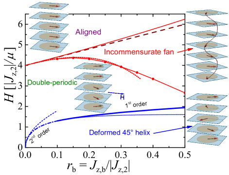
Figure 2: Magnetic phase diagram of the rotationally-isotropic model. The dotted blue line shows instability field of the double-periodic state, Eq. (24), which coincides with the second-order transition line for $r_{b}<0.099$ (dash-dotted line). The dashed line shows the low-$r_{b}$ asymptotics of this line, Eq. (25). The blue solid line at higher $r_{b}$ shows the location of the first-order transition to the double-periodic state. The upper red solid line shows the transition between the saturated and incommensurate fan states. The red dotted line shows the approximate transition line from incommensurate to double-periodic state obtained from Eq. (42). The solid red line with circles shows the more accurate transition line obtained by numerical minimization of the energy in Eq. (29) with respect to the fan state parameters. For comparison, the nominal saturation field for the double-periodic state is shown by the brown dashed line.

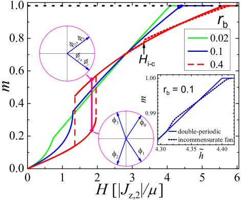
Figure 3: The representative magnetic-field dependences of the reduced magnetization for the rotationally-degenerate system for different values of the ratio $r_{b}=J_{z,b}/|J_{z,2}|$. The vertical solid line for $r_{b}\!=\!0.4$ shows the location of the $1^{\mathrm{st}}$-order phase transition and the picture insets show the computed spin configurations at the transition point. The dotted lines for $r_{b}\!=\!0.4$ and for $r_{b}\!=\!0.1$ in the inset show the magnetization for the incommensurate fan state. In the main plot, the range of this state for $r_{b}\!=\!0.1$ is marked by bold line. For reference, the solid lines showing the magnetization for the double-periodic state are extended to the high-field region where this state does not minimize the energy any more. For $r_{b}=0.02$ the range of incommensurate fan state is invisible in this scale.

Figure 2 summarizes the magnetic phase diagram in the $r_{b}$-$\tilde{h}$ plane for the model with rotational degeneracy. With increasing field, the system transforms from the deformed 45^∘ helix into the double-periodic state at the field monotonically increasing with the ratio $r_{b}=J_{z,b}/|J_{z,2}|$. At $r_{b}<r_{0}$, Eq. (27), the transition is second order at the field in Eq. (24). At higher $r_{b}$, the transition becomes first order and the second-order-transition line extends into the dotted instability line. The first-order line is obtained by direct numerical comparison of the energies in Eqs. (5) and (18) minimized with respect to the corresponding angles.

Further increase of the magnetic field leads to the transition from the double-periodic into incommensurate fan state. We show two approximate results for the boundary between two states. The red dotted line shows the analytical result in Eq. (42) valid for small $r_{b}$. The solid line with circles is obtained by numerical minimization of the energy in Eq. (29) with respect to fan states with different amplitudes and wave vectors. This procedure also provides independent numerical verification that the double-periodic state has the lowest energy in the intermediate field range. Finally, at even higher magnetic field, the continuous transition to the saturated aligned state takes place.

Figure 3 shows the representative magnetic-field dependences of the magnetization for different values of the ratio $r_{b}$. The solid lines are obtained for the symmetric states by minimizing the energy in Eq. (5) with respect to the angles $\alpha$ and $\beta$. The magnetization is then computed from Eq. (7). The dotted curves for $r_{b}=0.4$ in the main plot and for $r_{b}=0.1$ in the inset correspond to the incommensurate state. They are computed by minimizing the energy in Eq. (29) with respect to the fan amplitude $\vartheta$ and wave vector $q$. The magnetization is evaluated using the derivative of the energy with respect to the magnetic field. We see that the low-field behavior is characterized by upward curvature which becomes more pronounced at smaller $r_{b}$. The transition to the double-periodic state leads to noticeable features in the magnetization curves. At small $r_{b}$ the transition is manifested by a kink which becomes more pronounced with increasing $r_{b}$, while at high $r_{b}$, a kink is replaced with a first-order jump. With further increase of the field, the transition to the incommensurate-fan state takes place, which is accompanied by a small increase of the magnetization in comparison with the double-periodic state. With decreasing $r_{b}$, this increase becomes weaker and the field range for incommensurate state rapidly shrinks. At higher fields the magnetization drops below the double-periodic curve. Finally, the transition to the aligned state takes place at the saturation field, which monotonically increases with $r_{b}$. This transition is manifested as a kink in the magnetization curve. We also note that all curves intersect at one point. This feature occurs to be universal and we will discuss it in detail below.

III Finite four-fold anisotropy

In this section, we explore the magnetic phase diagram for finite in-plane four-fold anisotropy parameter $K_{4}$ using the full energy functional in Eq. (2). For a state with four-spin periodicity, this reduced energy per spin, $E_{s}=\mathcal{E}_{\mathrm{lay}}/N|J_{z,2}|$, can be written as

$$E_{s} =\frac{1}{2}\left[\cos\left(\phi_{2}\!-\!\phi_{0}\right)+\cos\left(\phi_{3}\!-\!\phi_{1}\right)\right]+\frac{k_{4}}{16}\sum_{n=0}^{3}\!\cos\left(4\phi_{n}\right)$$

$$+ \frac{r_{b}}{4}\left[\cos^{2}\left(\phi_{1}\!-\!\phi_{0}\right)\!+\!\cos^{2}\left(\phi_{2}\!-\!\phi_{1}\right)\right.$$

$$+ \left.\!\cos^{2}\left(\phi_{3}\!-\!\phi_{2}\right)\!+\!\cos^{2}\left(\phi_{0}\!-\!\phi_{3}\right)\right]\!-\frac{\tilde{h}}{4}\sum_{n=0}^{3}\!\cos\left(\phi_{n}\!-\!\theta\right).$$ (43)

This energy has the symmetry property

$$E_{s}(\phi_{n},\theta,k_{4})=E_{s}(\phi_{n}+\frac{\pi}{4},\theta+\frac{\pi}{4},-k_{4}),$$ (44)

i. e., the 45^∘ rotation is equivalent to sign change of the parameter $k_{4}$. Similar to the in-plane isotropic case, four-layer periodicity is violated in the vicinity of the saturation field.

The model in Eq. (43) assumes zero nearest-neighbor exchange constant $J_{z,1}$. As noted in the introduction, finite four-fold anisotropy stabilizes the 90^∘ helix within some range of this constant. This range is evaluated in Appendix A. Finite small $J_{z,1}$ does not significantly alter most results of this section. One key parameter which may be substantially affected by finite $J_{z,1}$ is the wave vector of the incommensurate-fan state near the saturation field, see Eq. (33). Influence of $J_{z,1}$ on this wave vector is evaluated in Appendix D.

The four-fold anisotropy fixes the orientation of the helix in zero magnetic field. For $k_{4}>0$ and $\tilde{h}=0$, the equilibrium angle configuration following from the energy in Eq. (43) is $\phi_{n}\!=\!\pi/4\!\mp\!\pi(n\!-\!1)/2$. This determines the four easy-axis directions in the $xy$ plane, at $\pm 45^{\circ}$ and $\pm 135^{\circ}$. In this case, the behavior is sensitive to the in-plane orientation of the magnetic field. In the following sections, we consider the phase diagrams for the two symmetric field orientations, 45^∘ with respect to the initial moment direction [$\theta\!=\!0$ in Eq. (43)] and along this direction ($\theta\!=\!45^{\circ}$).

III.1 Field angle 45^∘ with respect to easy axis

When the field is oriented at 45^∘ with respect to equilibrium moment direction, the behavior is qualitatively similar to the case $k_{4}\!=\!0$ with quantitative modifications of the typical fields and critical parameters caused by the finite anisotropy. Therefore, we follow the same route as in Sec. II and just revise the results accounting for the finite value of $k_{4}$. For the finite anisotropy, the energy of the symmetric state with angles defined in Eq. (4) becomes

$$E_{s}\left(\alpha,\beta\right)=\frac{r_{b}}{2}-\cos\left(\beta\!-\!\alpha\right)\!+\frac{r_{b}\!+\!k_{4}}{8}\left[\cos\left(4\alpha\right)\!+\!\cos\left(4\beta\right)\right]$$

$$+\frac{r_{b}}{4}\cos\left[2\left(\beta\!+\!\alpha\right)\right]-\frac{\tilde{h}}{2}\left(\cos\alpha\!-\!\cos\beta\right).$$ (45)

This gives equations for the equilibrium angles $\alpha$ and $\beta$

$$2\sin\left(\beta\!-\!\alpha\right) \!+\!k_{4}\sin(4\alpha)\!+\!r_{b}\left\{\sin(4\alpha)\!+\!\sin\left[2\left(\alpha\!+\!\beta\right)\right]\right\}\ \ \$$

$$-\tilde{h}\sin\alpha\!=\!0,$$ (46a)

$$2\sin\left(\beta\!-\!\alpha\right) \!-\!k_{4}\sin(4\beta)\!-\!r_{b}\left\{\sin(4\beta)\!+\!\sin\left[2\left(\alpha\!+\!\beta\right)\right]\right\}\ \ \$$

$$-\tilde{h}\sin\beta=\!0.$$ (46b)

First, we consider the small-$\tilde{h}$ expansion of the energy, similar to Eq. (12). The calculation details of the expansion of the angles and energy are presented in Appendix C.1 and the result for the energy is

$$E_{s}(\tilde{h})\approx-1-\frac{k_{4}}{4}-\frac{\tilde{h}^{2}}{16\left(1\!+\!r_{b}\!+\!k_{4}\right)}$$

$$- \frac{1}{512\left(2r_{b}\!+\!k_{4}\right)\!\left(1\!+\!r_{b}\!+\!k_{4}\right)^{2}}\!\left[1\!+\!\frac{\left(2r_{b}\!+\!k_{4}\right)\!\left(r_{b}\!+\!k_{4}\right)}{\left(1+r_{b}+k_{4}\right)^{2}}\right]\!\tilde{h}^{4}.$$ (47)

Contrary to the case considered in Sec. II, the rotational degeneracy of helix is already broken at zero magnetic field. Helix orientation considered in this subsection is favored by both the four-fold anisotropy and magnetic field. We will use this energy expansion later, in the consideration of the helix-rotation transition for different field orientation. The energy expansion in Eq. (47) gives the low-field behavior of the magnetization,

$$m(\tilde{h})\approx\frac{\tilde{h}}{8\left(1\!+\!r_{b}\!+\!k_{4}\right)}$$

$$+ \frac{1}{128\left(2r_{b}\!+\!k_{4}\right)\!\left(1\!+\!r_{b}\!+\!k_{4}\right)^{2}}\!\left[1\!+\!\frac{\left(2r_{b}\!+\!k_{4}\right)\!\left(r_{b}\!+\!k_{4}\right)}{\left(1+r_{b}+k_{4}\right)^{2}}\right]\!\tilde{h}^{3}.$$ (48)

We see that the four-fold anisotropy decreases the linear susceptibility. It also reduces the upward curvature. Similarly to the rotationally-degenerate case, at sufficiently high magnetic field the system transfers into the double-periodic state defined by Eq. (17). In the next subsection, we consider the influence of the four-fold anisotropy on this state.

III.1.1 Double-periodic state

For the finite four-fold anisotropy, the energy of the double-periodic state for considered field direction becomes

$$E_{s}\left(\alpha,\pi\!-\!\alpha\right) =\frac{r_{b}}{2}-\frac{k_{4}}{4}+\cos\left(2\alpha\right)+\frac{r_{b}\!+\!k_{4}}{2}\cos^{2}\left(2\alpha\right)$$

$$-\tilde{h}\cos\alpha$$ (49)

yielding the equation for the equilibrium angle

$$4\cos\alpha_{0}\left[1\!+\!\left(r_{b}\!+\!k_{4}\right)\cos\left(2\alpha_{0}\right)\right]-\tilde{h} =0.$$ (50)

For the double-periodic state, the magnetization would reach saturation at the field $\tilde{h}_{\mathrm{sat}}\!=\!4\left(1\!+\!r_{b}\!+\!k_{4}\right)$. However, as in the isotropic case, the double-periodic state transforms into the incommensurate fan with increasing magnetic field and therefore this field does not have a direct physical meaning. A peculiar property following from Eq. (50) is the presence of the universal point at the field $\tilde{h}\!=\!2\sqrt{2}$, where $\alpha_{0}\!=\!\pi/4$ and the neighboring moment pairs are orthogonal. The key observation is that the magnetization at this point $m\!=\!\sqrt{2}/2$ does not depend on the material’s parameters $r_{b}$ and $k_{4}$.

To evaluate stability of the state, we consider deviation from double periodicity, $\alpha=\alpha_{0}+\psi$, $\beta=\pi-\alpha_{0}+\psi$. Expansion of the energy in Eq. (45) with respect to $\psi$,

$$\delta E_{s}^{(2)}\left(\psi\right)\!=\!\left\{2\left[k_{4}\!-\!2(r_{b}\!+\!k_{4})\cos^{2}\left(2\alpha_{0}\right)\right]\!+\!\frac{\tilde{h}}{2}\cos\alpha_{0}\right\}\psi^{2}$$

gives the stability condition

$$4\left[k_{4}-2(r_{b}+k_{4})\cos^{2}\left(2\alpha_{0}\right)\right]+\tilde{h}\cos\alpha_{0}>0,$$ (51)

which determines the instability field $\tilde{h}_{i}$. Combining this result with the relation $\tilde{h}\cos\alpha_{0}\!=\!2\left[1\!+\!\cos\left(2\alpha_{0}\right)\right]\left[1\!+\!\left(r_{b}\!+\!k_{4}\right)\cos\left(2\alpha_{0}\right)\right]$ following from Eq. (50), we obtain a quadratic equation for $\cos\left(2\alpha_{0}\right)$

$$\left[1\!+\!\cos\left(2\alpha_{0}\right)\right]\left[1\!+\!\left(r_{b}\!+\!k_{4}\right)\cos\left(2\alpha_{0}\right)\right]$$

$$=\!4(r_{b}\!+\!k_{4})\cos^{2}\left(2\alpha_{0}\right)\!-\!2k_{4},$$

from which we obtain

$$\cos\left(2\alpha_{0}\right) =-\frac{2(1+2k_{4})}{1+r_{b}+k_{4}+\mathcal{R}},$$ (52)

$$\mathcal{R} =\left[\left(1\!+\!r_{b}\!+\!k_{4}\right)^{2}\!+\!12(1\!+\!2k_{4})(r_{b}\!+\!k_{4})\right]^{1/2}$$

giving

$$\cos\alpha_{0}\!= \frac{\left[6(1\!+\!2k_{4})(r_{b}\!+\!k_{4})\!+\!\left(1\!+\!r_{b}\!+\!k_{4}\right)\left(r_{b}\!-\!k_{4}\right)\!+\!\left(r_{b}\!-\!k_{4}\right)\mathcal{R}\right]^{1/2}}{1+r_{b}+k_{4}+\mathcal{R}}.$$

These results allow us to obtain the instability field for finite anisotropy from Eq. (51),

$$\tilde{h}_{i}(r_{b},k_{4})=4\cos\alpha_{0}\left[1+\left(r_{b}+k_{4}\right)\cos\left(2\alpha_{0}\right)\right]$$ (53)

$$=4\frac{\left[6(1\!+\!2k_{4})(r_{b}\!+\!k_{4})\!+\!\left(r_{b}\!-\!k_{4}\right)\left(1\!+\!r_{b}\!+\!k_{4}\!+\!\mathcal{R}\right)\right]^{1/2}\left[1\!-\!\left(r_{b}\!+\!k_{4}\right)\left(1\!+\!4k_{4}\right)\!+\!\mathcal{R}\right]}{\left[1+r_{b}+k_{4}+\mathcal{R}\right]^{2}}.$$

For $k_{4}\!=\!0$ this result reproduces Eq. (24). The double-periodic state is stable at $\tilde{h}>\tilde{h}_{i}(r_{b},k_{4})$. In general, the four-fold anisotropy affects the instability field in rather complicated way. In the expected case of small parameters, $r_{b},k_{4}\ll 1$, the instability field has a simple asymptotics

$$\tilde{h}_{i}(r_{b},k_{4})\simeq 4\sqrt{2r_{b}+k_{4}}.$$ (54)

We see that at small $r_{b}$, the four-fold anisotropy increases the instability field. However, the accurate analysis shows that this is only correct for $r_{b}<0.09$.

The nature of the phase transitions between the deformed 45^∘ helix and double-periodic states is determined by the sign of the quartic-term coefficient $c_{4}$ in the energy expansion with respect to the perturbation $\psi$, $\delta E_{s}^{(4)}=\frac{1}{4}c_{4}\psi^{4}$. The calculation of this quartic coefficient described in Appendix C.2 yields the result

$$c_{4}(r_{b},k_{4})\! =\!20\left(r_{b}\!+\!k_{4}\right)u^{2}\!-\!10k_{4}\!$$

$$- \frac{\left(1\!-\!u^{2}\right)\left(1\!+\!15\left(r_{b}\!+\!k_{4}\right)u\right)^{2}}{2\left(u+r_{b}\right)},$$ (55)

$$u= -\cos\left(2\alpha_{0}\right)=\frac{2(1+2k_{4})}{1\!+\!r_{b}\!+\!k_{4}\!+\!\mathcal{R}},$$

where the parameter $\mathcal{R}$ is defined in Eq. (52). At small $r_{b}$ and $k_{4}$, the quartic coefficient is positive corresponding to the second-order phase transition. The transition becomes first order with increasing of either $r_{b}$ or $k_{4}$. The boundary $c_{4}(r_{b},k_{4})=0$ is shown by the navy line in the Fig. 4. It is very close to the linear dependence, $r_{0}(k_{4})\approx 0.099-1.22k_{4}$. We see that the critical value of $r_{b}$, where the nature of the transition changes, decreases with increasing $k_{4}$ and for $k_{4}>0.081$ the transition is first order for any $r_{b}$.

As in the rotationally-isotropic case, the double-periodic state transforms into the incommensurate fan, Eq. (28), in the vicinity of the saturation field. In the next subsection, we consider the latter state in the case of finite four-fold anisotropy.

III.1.2 Influence of four-fold anisotropy on incommensurate-fan state near saturation

In this subsection, we consider modifications of the incommensurate-fan state caused by the finite four-fold anisotropy term, $K_{4}\left(\cos^{4}\phi_{n}\!+\!\sin^{4}\phi_{n}\!-\frac{3}{4}\right),$ in the energy functional, Eq. (2). In this case, the fan energy, Eq. (29) has the additional term $\frac{1}{N}\sum_{n}\frac{k_{4}}{4}\cos\left[4\vartheta\sin\left(qn+\varphi\right)\right]$. As a consequence, the quadratic term in the energy expansion with respect to the fan amplitude $\vartheta$, Eq. (32), acquires additional $q$-independent contribution

$$a_{2}\left(q\right) =\!-2k_{4}\!-\!2\sin^{2}q\!-\!2r_{b}(1\!-\!\cos q)\!+\!\frac{\tilde{h}}{2}.$$ (56)

This means that the four-fold anisotropy just increases the saturation field,

$$\tilde{h}_{sat}=(2+r_{b})^{2}+4k_{4}$$ (57)

but does not change much the overall behavior. In particular, the energy minimum is still realized at the wave vector in Eq. (33). However, as mentioned above, finite four-fold anisotropy stabilizes 90^∘ helix for some range of the nearest-neighbor exchange interaction constant $J_{z,1}$ and this constant does affect the wave vector of the incommensurate-fan state, see Appendix D. Importantly, with finite $J_{z,1}$, the period of this state can be both smaller and larger than four layers.

For the quartic coefficient, we obtain

$$a_{4}\left(q\right)\!=\!\sin^{4}q\!+\!2r_{b}\left(1\!-\!\cos q\right)^{2}\!+\!4k_{4}\!-\!\frac{\tilde{h}}{16}$$ (58)

for $q\neq\frac{\pi}{2},\pi$ and

$$a_{4}\left(\frac{\pi}{2},\varphi\right)\! =\!1\!+\!2r_{b}\!+\!4k_{4}\!-\!\frac{\tilde{h}}{16}$$

$$+ \frac{1}{3}\left(1\!-\!2r_{b}\!+\!4k_{4}\!-\frac{\tilde{h}}{16}\right)\cos\left(4\varphi\right).$$ (59)

From the above quadratic and quartic coefficients in Eqs. (56) and (58), we find that the energy of the incommensurate state below the saturation field, Eq. (38), is modified as

$$E_{\mathrm{fan}}\left(q\right)=1+r_{b}+\frac{k_{4}}{4}-\tilde{h}$$

$$-\frac{\left[\sin^{2}q+r_{b}\left(1\!-\!\cos q\right)+k_{4}-\frac{\tilde{h}}{4}\right]^{2}}{\sin^{4}q+2r_{b}\left(1\!-\!\cos q\right)^{2}+4k_{4}\!-\tilde{h}/16}.$$ (60)

For small $r_{b}$, near instability one can again neglect the field dependence of the optimal wave vector $q$ and use $\cos Q=-\frac{r_{b}}{2}$ from Eq. (33) yielding

$$E_{\mathrm{fan}}\left(Q\right)\approx 1+r_{b}+\frac{k_{4}}{4}-\tilde{h}$$

$$-\frac{\left[\left(1+\frac{r_{b}}{2}\right)^{2}+k_{4}-\frac{\tilde{h}}{4}\right]^{2}}{\left(1+\frac{r_{b}}{2}\right)^{4}+4k_{4}-\tilde{h}/16}.$$ (61)

On the other hand, for the state with $q=\pi/2$ we have

$$E_{\mathrm{fan}}\left(\pi/2,\varphi\right)=1+r_{b}+\frac{k_{4}}{4}-\tilde{h}$$

$$-\frac{\left(1+r_{b}+\frac{k_{4}}{4}-\frac{\tilde{h}}{4}\right)^{2}}{1\!+\!2r_{b}\!+\!4k_{4}\!-\!\frac{\tilde{h}}{16}+\frac{1}{3}\left[1\!-\!2r_{b}\!+\!4k_{4}\!-\frac{\tilde{h}}{16}\right]\cos\left(4\varphi\right)}.$$ (62)

For $1-2r_{b}+4k_{4}-\tilde{h}/16>0$ or, at the instability field, $3r_{b}-5k_{4}<1$, minimum energy is realized for the double-periodic state, $\varphi\!=\!\pi/4$, yielding

$$E_{\mathrm{fan}}\left(\pi/2,\pi/4\right) =1+r_{b}+\frac{k_{4}}{4}-\tilde{h}.$$

$$- \frac{3\left(1+r_{b}+k_{4}-\frac{\tilde{h}}{4}\right)^{2}}{2+8r_{b}+8k_{4}-\tilde{h}/8}.$$ (63)

Comparing the energies of two states in Eqs. (61) and (63), we can estimate the transition field in the limit $r_{b}\ll 1$

$$\tilde{h}_{\mathrm{i-c}}\approx 4\left(1\!+\!r_{b}\!+\!k_{4}\right)$$

$$-2\left(\sqrt{\frac{3}{2}}\!+\!1\right)\left[1\!+\!4\left(1\!+\!\sqrt{\frac{2}{3}}\right)\frac{r_{b}}{1\!+\!5k_{4}}\right]r_{b}^{2}.$$ (64)

From this result and the value of the saturation field in Eq. (57), we can conclude that the field range of the incommensurate state is still proportional to $r_{b}^{2}$ and the four-fold anisotropy has only a small influence on this range.

III.2 Field along easy axis

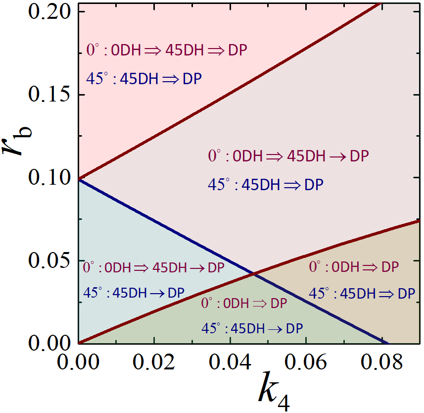
Figure 4: The parameter regions with different spin-state-transformations scenarios for two field orientations. Here 0DH, 45DH, and DP stand for deformed 0^∘ helix, deformed 45^∘ helix, and double-periodic state, respectively, see Fig. 1. Single ($\rightarrow$) and double ($\Rightarrow$) arrows indicate to a second- and first-order phase transitions, respectively. The upper brown and navy line corresponds to change from second- to first-order transition to the DP state for the magnetic field applied along the easy axis and at 45^∘, respectively. Above the lower brown line, for the easy-axis field direction, the system first has the helix-rotation transition from 0DH to 45DH state and then transfers into the DP state. Below this line, the system jumps directly from 0DH to DP state bypassing the intermediate 45DH state.

The case of field along the equilibrium moment direction is richer and more complicated than the previous cases. The reason is that for such field direction, the interaction with the field and the four-fold anisotropy favor different helix orientations. For $\theta=\pi/4$ in Eq. (43), it is convenient to utilize the symmetry property in Eq. (44) and make substitution $\phi_{n}\rightarrow\phi_{n}+\pi/4$ which transforms the energy to the same form as for $\theta=0$ except for the sign reverse in the $k_{4}$ term. Therefore, after this substitution, the energy per spin becomes

$$E_{s} =\frac{1}{2}\left[\cos\left(\phi_{2}\!-\!\phi_{0}\right)+\cos\left(\phi_{3}\!-\!\phi_{1}\right)\right]\!-\frac{k_{4}}{16}\sum_{n=0}^{3}\cos\left(4\phi_{n}\right)$$

$$+ \frac{r_{b}}{4}\left[\cos^{2}\left(\phi_{1}\!-\!\phi_{0}\right)\!+\!\cos^{2}\left(\phi_{2}\!-\!\phi_{1}\right)\right.$$

$$+\! \left.\cos^{2}\left(\phi_{3}\!-\!\phi_{2}\right)+\cos^{2}\left(\phi_{0}\!-\!\phi_{3}\right)\right]\!-\!\frac{\tilde{h}}{4}\sum_{n=0}^{3}\!\cos\left(\phi_{n}\right).$$ (65)

At low magnetic fields, the ground state is given by the deformed 0^∘ helix abbreviated as 0DH (lower 3D picture in Fig. 1), which is described by the angles $\phi_{0}=0$, $\phi_{3}=-\phi_{1}=\alpha$, $\phi_{2}=\pi$. Its energy is given by

$$E_{s} =\frac{1}{2}\left[-1+\cos\left(2\alpha\right)\right]-\frac{k_{4}}{8}\left[1+\cos\left(4\alpha\right)\right]$$

$$+r_{b}\cos^{2}\alpha-\frac{\tilde{h}}{2}\cos\alpha$$ (66)

and the equilibrium angle $\alpha_{0}$ is determined by the equation

$$4\cos\alpha_{0}\left[1+r_{b}-k_{4}\cos\left(2\alpha_{0}\right)\right]-\tilde{h}=0.$$ (67)

Using substitution $u=\cos\alpha_{0}$, we rewrite these equations as

$$E_{s} =-1-\frac{k_{4}}{4}+\left(1+r_{b}+k_{4}\right)u^{2}-k_{4}u^{4}-\frac{\tilde{h}}{2}u,$$ (68a)

$$4u\left[1+r_{b}+k_{4}-2k_{4}u^{2}\right]=\tilde{h}.$$ (68b)

Contrary to isotropic case, the second equation does not have a compact analytical solution similar to Eq. (15a). We start with the analytic analysis of helix configuration at small magnetic field.

III.2.1 Small $\tilde{h}$ expansion and first-order helix-rotation transition

At small magnetic field, we derive from Eq. (68b) the expansion of the parameter $u$ with respect to $\tilde{h}$,

$$u\! \approx\frac{\tilde{h}}{4\left(1\!+\!r_{b}\!+\!k_{4}\right)}+\frac{k_{4}\tilde{h}^{3}}{32\left(1\!+\!r_{b}\!+\!k_{4}\right)^{4}}.$$

Substituting this result into Eq. (68a), we obtain the expansion of the energy

$$E_{s}(\tilde{h})\!\approx\!-1\!-\frac{k_{4}}{4}-\frac{\tilde{h}^{2}}{16\left(1\!+\!r_{b}\!+\!k_{4}\right)}-\frac{k_{4}\tilde{h}^{4}}{256\left(1\!+\!r_{b}\!+\!k_{4}\right)^{4}},$$ (69)

which determines the low-field behavior of the magnetization

$$m(\tilde{h})\approx\frac{\tilde{h}}{8\left(1\!+\!r_{b}\!+\!k_{4}\right)}+\frac{k_{4}\tilde{h}^{3}}{64\left(1\!+r_{b}\!+k_{4}\right)^{4}}.$$ (70)

Comparing the cubic terms in this result and in Eq. (48), we can conclude that the small-field magnetization for the easy-axis direction is lower than for the 45^∘ direction.

As demonstrated in Sec. II, the magnetic field favors the 45^∘ helix orientations, which conflicts with the initial parallel orientation set by the four-fold anisotropy. Therefore, at small $k_{4}$, a sufficiently strong magnetic field should reorient the helix. This rotation transition is somewhat similar to the spin-flop transition in easy-axis antiferromagnets for the magnetic field applied along the easy axis, see, e. g., Ref. [35]. To find the field at which such helix-rotation spin-flop transition takes place, $\tilde{h}_{r}$, we have to compare the energy of the 0^∘ helix in Eq. (69) with the energy of the 45^∘ helix, which in our case can be obtained from Eq. (47) with the substitution $k_{4}\rightarrow-k_{4}$. In the limit $k_{4}\ll 1$, we can neglect $k_{4}$ in the field-dependent terms. This gives transition field in the lowest order with respect to $k_{4}$,

$$\tilde{h}_{r}\simeq 4\left(1+r_{b}\right)\left[\frac{2r_{b}k_{4}}{1+2r_{b}+3r_{b}^{2}}\right]^{1/4}.$$ (71)

In particular, $\tilde{h}_{r}\!\simeq\!4\left[2r_{b}k_{4}\right]^{1/4}$ for $r_{b},k_{4}\ll 1$. This corresponds to $\mu H_{r}\!\simeq\!4\left[2J_{z,b}K_{4}\right]^{1/4}\!\sqrt{|J_{z,2}|}$ in real units. Keeping $k_{4}$ in the expansion terms, we can derive a somewhat more accurate result with the next-order term,

$$\tilde{h}_{r}\!\simeq 4\left(1\!+r_{b}\right)\left(\frac{2r_{b}k_{4}}{1\!+\!2r_{b}\!+\!3r_{b}^{2}}\right)^{1/4}$$

$$\times \!\left(1\!-\!\sqrt{\frac{2r_{b}k_{4}}{1\!+\!2r_{b}\!+3r_{b}^{2}}}\right).$$ (72)

When $k_{4}$ is not very small, the precise location of transition can be found numerically by the energy comparison. With further increase of the magnetic field, the system again transforms into the double-periodic state. In addition, the accurate analysis shows that at sufficiently large $k_{4}$ the intermediate 45DH state may be bypassed and the 0DH state may jump directly into the DP state.

III.2.2 Double-periodic and incommensurate-fan states

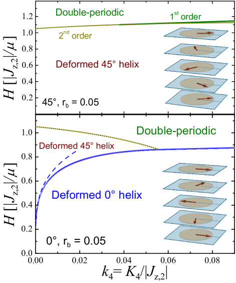
Figure 5: Phase diagrams in the plane four-fold anisotropy–magnetic field for the ratio $r_{b}=0.05$. The upper and lower panel is for the magnetic field oriented at 45^∘ and 0^∘ with respect to the equilibrium moment direction (easy axis). In former case, the transition field to the double-periodic state slowly increases with $k_{4}$ and the transition becomes first order at $k_{4}>0.0375$. For the parallel direction in the lower plot, the two subsequent transition 0DH$\Rightarrow$ 45DH$\rightarrow$DP are realized for $k_{4}<0.055$ and only one first-order transition 0DH$\rightarrow$DP is realized at higher $k_{4}$. The dashed line in the lower panel presents the low-$k_{4}$ asymptotics of the rotation transition field $\tilde{h}_{r}$ given by Eq. (71).

In the DP state, the energy and the equation for the equilibrium angle can be obtained from Eq. (50) by replacement $k_{4}\rightarrow-k_{4}$,

$$E_{s}\left(\alpha,\pi-\alpha\right)=\cos\left(2\alpha\right)+\frac{k_{4}}{4}$$

$$+\frac{r_{b}}{2}+\frac{r_{b}-k_{4}}{2}\cos^{2}\left(2\alpha\right)-\tilde{h}\cos\alpha,$$ (73a)

$$4\cos\alpha_{0}\left[1+\left(-k_{4}+r_{b}\right)\cos\left(2\alpha_{0}\right)\right]-\tilde{h}=0.$$ (73b)

Similarly, the instability field for the double-periodic state $\tilde{h}_{i}$ and the quartic coefficient $c_{4}$ for this field direction can be obtained from Eqs. (53) and (55) with the same replacement $k_{4}\!\rightarrow\!-k_{4}$. In particular, at small $r_{b}$ the four-fold anisotropy reduces the instability field for the easy-axis orientation. The parameter range where the 45DH $\rightarrow$ DP transition changes its order is now determined by the condition $c_{4}(r_{b},-k_{4})=0$ using Eq. (55). For the easy-axis field direction, the critical value of $r_{b}$ above which the transition becomes first order increases with $k_{4}$. This critical value is shown in Fig. 4 by the upper brown line.

At sufficiently large $k_{4}$, two subsequent phase transitions are replaced by a single first-order phase transition at which the system directly jumps from the 0DH to DP state. To find the parameter range where this scenario is realized, we find the field of such direct transition $\tilde{h}_{t}(r_{b},k_{4})$ by comparing the energies of two states in Eqs. (66) and (73a). The direct-transition scenario is realized when $\tilde{h}_{t}(r_{b},k_{4})>\tilde{h}_{i}(r_{b},-k_{4})$, where $\tilde{h}_{i}(r_{b},k_{4})$ is given by Eq. (53). At small $r_{b}$ and $k_{4}$ such direct first-order transition takes place for $k_{4}\!>\!1.04r_{b}$. The lower brown line in Fig. 4 shows the boundary below which the direct-transition scenario is realized.

As mentioned above, the universal point $\alpha_{0}\!=\!\pi/4$ is realized in the DP state at the field $\tilde{h}\!=\!2\sqrt{2}$, where magnetization $m\!=\!\sqrt{2}/2$ does not depend on $r_{b}$ and $k_{4}$. As a consequence, the magnetization is also identical for two field orientations, meaning that the magnetization curves $m(\tilde{h})$ always cross at this point.

As in other cases, the DP state transforms into the incommensurate-fan state at high fields. The results of subsection III.1.2 can be directly applied to the easy-axis orientation using the same substitution $k_{4}\!\rightarrow\!-k_{4}$. In particular, the saturation field for this orientation $\tilde{h}_{sat}=(2+r_{b})^{2}-4k_{4}$ is smaller than for the 45^∘ field orientation in Eq. (57), $\tilde{h}_{\mathrm{sat}}(45\text{\textdegree})\!-\!\tilde{h}_{\mathrm{sat}}(0\text{\textdegree})=8k_{4}$.

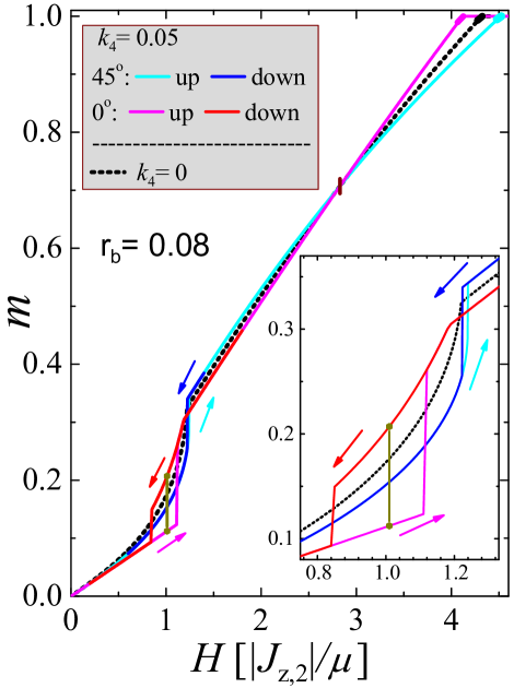
Figure 6: The representative field dependences of the magnetization for two field directions for parameters $r_{b}=0.08$ and $k_{4}=0.05$. The inset zooms into the transition’s regions. For comparison, we also show by the black dashed line the curve for rotationally-isotropic case, $k_{4}=0$. For both field orientations the kinks near $\tilde{h}=\mu H/|J_{z,2}|\approx 1.2$ correspond to the phase transitions from the deformed $45^{\circ}$ helix to double-periodic state. For the $0^{\circ}$ ($45^{\circ}$) orientation the anisotropy slightly decreased (increases) the transition field and for the $45^{\circ}$ orientation the transition becomes of the first order. For the parallel orientation, there is also the first-order phase transition near $\tilde{h}=\mu H/|J_{z,2}|\approx 1$ marked by the vertical line corresponding to the helix rotation, as illustrated in Fig. 1. All magnetization curves intersect at the point $\tilde{h}=\mu H/|J_{z,2}|=2\sqrt{2},$ $m=\sqrt{2}/2$ marked by the vertical bar. The bold lines near the saturation show the regions occupied by the incommensurate-fan state.

III.3 Phase diagrams and magnetization curves

Figure 5 shows the phase diagrams in the $k_{4}$-$\tilde{h}$ plane for $r_{b}=0.05$ and two field orientations for fields significantly lower than the saturation region. The upper and lower panel is for angle 45^∘ and 0^∘ between the magnetic field and the equilibrium moment direction, respectively. In the former case, the transition field to the double-periodic state slowly increases with $k_{4}$. The transition becomes first order at $k_{4}>0.0375$. In the lower panel, the two subsequent transition 0DH$\Rightarrow$ 45DH$\rightarrow$DP are realized at small $k_{4}$ with opposite dependences of the transition fields on $k_{4}$. At $k_{4}=0.055$ the transition lines cross and only one first-order transition 0DH$\rightarrow$DP is realized at higher $k_{4}$. The dashed line in the lower panel presents the low-$k_{4}$ asymptotics of the rotation transition field $\tilde{h}_{r}$ given by Eq. (71). We can see that it gives an accurate estimate of the transition field only at very small $k_{4}$, $k_{4}\lesssim 0.01$.

Figure 6 shows the field dependences of the magnetization curves for the two field orientations. The plots are made using the representative parameters $r_{b}=0.08$ and $k_{4}=0.05$. The curve for 45^∘ orientation is obtained in a way similar to $k_{4}\!=\!0$ case in Fig. 3. For 0^∘ orientation, we minimized the energy in Eq. (65) with respect to four angles $\phi_{i}$. In this case, we found that the ground-state configuration always corresponds to one of the symmetric states shown in Fig. 1. One can observe several key features. Both field orientations are characterized by the transition to the DP state near $\tilde{h}\approx 1.2$. For the 45^∘ orientation the transition is weak first-order one and is located at a somewhat higher field than for the parallel orientation. In addition, for the easy-axis orientation, the first-order helix rotation transition takes place at a somewhat lower field, near $\tilde{h}\approx 1$. The magnetization curves for the two field orientations cross three times: at smallest fields, the magnetization is lower for the easy-axis direction, it becomes larger for this direction after the first-order transition into the 45DH state and it remains larger until the transition into the DP state. Note that this small field range is not universal and vanishes for larger $k_{4}$. In the DP state, the magnetization is again lower for the easy-axis direction until two magnetization curves cross at the universal point $\tilde{h}=2\sqrt{2}$.

In both cases, there are narrow incommensurate-fan regions near the saturation. These regions are marked by bold lines in the plot. Small modifications of the magnetization in these regions are similar to one shown in the inset of Fig. 3. Finally, the magnetization in the easy-axis direction saturates at a smaller magnetic field than for the 45^∘ orientation. Qualitatively, these generic shapes of magnetization curves realize for other sets of parameters and their features can be used for experimental determination of the equilibrium helix orientation at zero magnetic field.

IV Summary and discussion

In summary, we investigated a phenomenological phase diagram for the magnetic helical state with a 90^∘ turn angle between neighboring spin layers in the external magnetic field applied perpendicular to the helix axis. We assumed that this unusual state is stabilized by the biquadratic nearest-neighbor interaction and in-plane four-fold anisotropy. We found the metamagnetic transition from the distorted helix into the double-periodic state. The corresponding transition field is mostly determined by the strength of the biquadratic interaction. In addition, this field depends on the four-fold anisotropy and field orientation. Depending on the parameters, the transition to the double-periodic state can be either second or first order. Such behavior is different from the helical structures realized within the frustrated Heisenberg model, where the nature of the transition is fully determined by the modulation wave vector [12]. When the magnetic field is applied along the equilibrium moment direction (easy axis) and the four-fold anisotropy $K_{4}$ is weak, we found an additional first-order spin-flop transition corresponding to the 45^∘ rotation of the distorted helix. The field of this transition behaves as $K_{4}^{1/4}$ for $K_{4}\rightarrow 0$. At sufficiently large $K_{4}$, this helix rotation is bypassed and there is only one first-order spin-flop transition directly into the double-periodic state.

In the vicinity of the saturation field, the double-periodic state transforms into the incommensurate fan. The field range of the latter state is proportional to the biquadratic coupling squared. In the model with rotational degeneracy, the fan period is always smaller than four layers. On the other hand, for the model with the four-fold anisotropy and finite nearest-neighbor exchange constant, the period may be both smaller and larger than four layers. Interestingly, recent neutron-scattering results [36] suggest that, at high magnetic fields, the structure period becomes a little bit larger than four layers corresponding to the wave vector dropping below $\pi/2$.

We evaluated the phase diagrams within a mean-field theory completely neglecting thermal spin fluctuations. These fluctuations grow when the temperature approaches the magnetic transition point $T_{m}$. We expect that the transition magnetic fields computed here will be reduced by the spin fluctuations and vanish as $T\rightarrow T_{m}$. The fluctuations also may significantly modify the shapes of magnetization features at the transitions.

The unusual helical state considered in this paper has been established in the superconducting iron arsenide RbEuFe₄As₄[21, 20], which has the superconducting transition at 36.5 K and magnetic transition at 15K. The most likely reason for very small nearest-neighbor bilinear exchange interaction $J_{z,1}$ in this material is an accidental compensation of the normal and superconducting RKKY contributions to this parameter [34]. In addition, the biquadratic nearest-neighbor term probably has a superconducting origin due to sensitivity of the superconducting energy to the exchange field.

Since the interlayer helical state emerges inside the superconducting state, the global magnetic response is hidden either by superconducting screening or by the presence of superconducting vortex lines. This complicates direct verification of the predicted fine features in the magnetization. The magnetic field is not uniform in the superconducting state. In the Meissner state, it drops at the scale of the London penetration depth from the surface and in the equilibrium vortex state it oscillates with the periods given by vortex-lattice spacings. Even more severe disturbing factor is the formation of the critical state due to vortex pinning in which the magnetic field is macroscopically nonuniform. Due to the temperature dependence of the magnetic susceptibility, such state is formed even for cooling in fixed external magnetic field[37, *VlaskoVlasovPhysRevB.101.104504]. The distinct features in the global magnetization at the transition fields will be smeared because of these field spatial variations.

The magnetic field varies at spatial scales much larger than the distance between the Eu²⁺ moments. Therefore, in the simplest scenario, we expect that the local spin configuration and magnetization follow the local magnetic field. The saturation field for the in-plane orientation is about 1 kG [39]. The metamagnetic transition fields depend on the material’s parameters $K_{4}$ and $J_{b}$ that are currently unknown. As these parameters are expected to be small in comparison with $J_{z,2}$, it is feasible that the metamagnetic transition fields may be smaller than the in-plane lower critical field $H_{c1}^{ab}$, which for this material is roughly 200 G at low temperatures. In this case, even in the Meissner state, the magnetic behavior becomes nontrivial: the spin configuration at the surface will transform with increasing magnetic field and the boundary between two different spin states will be formed parallel to the surface. Similarly, the spin configuration near the center of an isolated in-plane vortex line will be different from the configuration outside and the vortex core will be surrounded by the boundary with the shape of an elliptical cylinder. Such unusual magnetic vortex structure may have a substantial influence on the properties of the vortex state. In particular, it may be relevant for the understanding of clustering instabilities found in RbEuFe₄As₄ by magnetooptical imaging of side faces [37, *VlaskoVlasovPhysRevB.101.104504].

Appendix A Range of stability of 90^∘ helix for finite nearest-neighbor exchange interaction

With finite nearest-neighbor coupling, the energy in Eq. (2) at zero magnetic field becomes

$$E_{s} =\frac{1}{N}\sum_{n}\Big{[}|J_{z,2}|\cos\left(\phi_{n+2}\!-\!\phi_{n}\right)-J_{z,1}\cos\left(\phi_{n+1}\!-\!\phi_{n}\right)$$

$$+ J_{z,b}\cos^{2}\left(\phi_{n+1}-\phi_{n}\right)+\frac{K_{4}}{4}\cos\left(4\phi_{n}\right)\Big{]}.$$ (74)

We find the range of $J_{z,1}$ within which 90^∘ helix still gives the ground state. Substituting the helix ansatz, $\phi_{n}=qn+\pi/4$, we obtain

$$E_{s}\left(q\right) =-|J_{z,2}|+\left(2|J_{z,2}|+J_{z,b}\right)\cos^{2}q$$

$$-J_{z,1}\cos q-\frac{K_{4}}{4}\left\langle\cos\left(4qn\right)\right\rangle_{n}.$$ (75)

For the incommensurate state, the four-fold anisotropy vanishes. In this case, we find the optimal wave vector

$$\cos Q=\frac{J_{z,1}}{2\left(2|J_{z,2}|\!+\!J_{z,b}\right)}$$ (76)

and the corresponding incommensurate-state energy

$$E_{s}\left(Q\right)=-|J_{z,2}|-\frac{J_{z,1}^{2}}{4\left(2|J_{z,2}|\!+\!J_{z,b}\right)}.$$ (77)

On the other hand, the energy of 90^∘ helix is

$$E_{s}\left(\pi/2\right)=-|J_{z,2}|\!-\frac{K_{4}}{4}.$$ (78)

Comparing energies in Eqs. (77) and (78), we find that the 90^∘ helix gives ground state if the condition

$$|J_{z,1}|<\sqrt{\left(2|J_{z,2}|\!+\!J_{z,b}\right)K_{4}}.$$ (79)

is satisfied. This result is approximate, because we limit ourselves by a simple incommensurate helical state and did not consider more complicated nonuniform configurations which may emerge at the transition.

Appendix B Calculation of quartic coefficient in the energy expansion for $k_{4}=0$

Presenting the angles as $\alpha=\alpha_{0}+\psi+\vartheta$, $\beta=\pi-\alpha_{0}+\psi-\vartheta$, we derive expansion of the energy in Eq. (5) with respect to $\psi$ and $\vartheta$

$$\delta E_{s}\left(\psi,\vartheta\right)\approx\left[-2\cos\left(2\alpha_{0}\right)-2r_{b}\cos\left(4\alpha_{0}\right)+\frac{\tilde{h}}{2}\cos\alpha_{0}\right]\vartheta^{2}$$

$$+\left[\!-4r_{b}\cos^{2}\left(2\alpha_{0}\right)\!+\frac{\tilde{h}}{2}\cos\alpha_{0}\!\right]$$

$$+\!\left(8r_{b}\sin 4\alpha_{0}\!-\frac{\tilde{h}}{2}\sin\alpha_{0}\right)\vartheta\psi^{2}$$

$$+\left[\frac{16}{3}r_{b}\cos^{2}\left(2\alpha_{0}\right)-\frac{\tilde{h}}{24}\cos\alpha_{0}\right]\psi^{4}$$

Excluding $\vartheta$ for fixed $\psi$

$$\vartheta=-\frac{8r_{b}\sin(4\alpha_{0})-\frac{\tilde{h}}{2}\sin\alpha_{0}}{-4\cos\left(2\alpha_{0}\right)-4r_{b}\cos\left(4\alpha_{0}\right)+\tilde{h}\cos\alpha_{0}}\psi^{2},$$

we obtain the full quartic term for expansion with respect to $\psi$

$$E_{s}^{(4)} =\frac{1}{4}c_{4}\psi^{4},$$

$$c_{4} =\frac{64}{3}r_{b}\cos^{2}\left(2\alpha_{0}\right)-\frac{\tilde{h}}{6}\cos(\alpha_{0})$$

$$- \frac{\left(8r_{b}\sin 4\alpha_{0}-\frac{\tilde{h}}{2}\sin\alpha_{0}\right)^{2}}{-2\cos\left(2\alpha_{0}\right)-2r_{b}\cos\left(4\alpha_{0}\right)+\frac{\tilde{h}}{2}\cos\alpha_{0}}.$$

At the instability point, we have relations given by Eqs. (19) and (21). This allows us to exclude both $\tilde{h}$ and $\alpha_{0}$ and express $c_{4}$ at the instability point via $r_{b}$ leading to Eq. (26) of the main text.

Appendix C Calculations for finite four-fold anisotropy and for field angle 45^∘ with respect to the moment direction

C.1 Small-$\tilde{h}$ expansion

We follow essentially the same steps as in derivation of expansion in Eq. (12). Small magnetic field leads to small deviations, which we represent as $\alpha\!=\!\frac{\pi}{4}\!-\!\alpha_{+}\!-\frac{\alpha_{-}}{2},\beta\!=\!\frac{\pi}{4}+\!\alpha_{+}\!-\frac{\alpha_{-}}{2}$. The energy can be expanded as

$$E_{s}\left(\alpha_{+},\alpha_{-}\right)\approx\!-1\!-\frac{k_{4}}{4}+\!2\left(1\!+\!r_{b}\!+\!k_{4}\right)\alpha_{+}^{2}\!+\!\left(2r_{b}\!+\!k_{4}\right)\frac{\alpha_{-}^{2}}{2}$$

$$-\frac{2\left[1\!+\!4\left(r_{b}\!+\!k_{4}\right)\right]\alpha_{+}^{4}}{3}-4\left(r_{b}\!+\!k_{4}\right)\alpha_{+}^{2}\alpha_{-}^{2}\!-\frac{1}{6}\left(2r_{b}\!+\!k_{4}\right)\alpha_{-}^{4}$$

$$-\frac{\sqrt{2}\tilde{h}}{4}\left(2\alpha_{+}-\alpha_{+}\alpha_{-}-\frac{1}{3}\alpha_{+}^{3}-\frac{1}{4}\alpha_{+}\alpha_{-}^{2}\right).$$ (80)

This gives equation for equilibrium $\alpha_{\pm}$

$$4\left(1\!+\!r_{b}\!+\!k_{4}\right)\alpha_{+}\!-\frac{8}{3}\left[1\!+\!4\left(r_{b}\!+\!k_{4}\right)\right]\alpha_{+}^{3}\!-\!8\left(r_{b}\!+\!k_{4}\right)\alpha_{+}\alpha_{-}^{2}$$

$$-\frac{\sqrt{2}\tilde{h}}{4}\left(2\!-\!\alpha_{-}\!-\!\alpha_{+}^{2}\!-\frac{1}{4}\alpha_{-}^{2}\right)=\!0,$$ (81a)

$$\left(2r_{b}+k_{4}\right)\alpha_{-}-8\left(r_{b}+k_{4}\right)\alpha_{+}^{2}\alpha_{-}-\frac{2}{3}\left(2r_{b}+k_{4}\right)\alpha_{-}^{3}$$

$$+\frac{\sqrt{2}\tilde{h}}{4}\left(\alpha_{+}+\frac{1}{2}\alpha_{+}\alpha_{-}\right)=\!0.$$ (81b)

In the expansion with respect to $\tilde{h}$,

$$\alpha_{\pm}=\sum_{n=1}^{\infty}\alpha_{\pm}^{(n)}\tilde{h}^{n},$$

only odd $\alpha_{+}^{(n)}$ and even $\alpha_{-}^{(n)}$ are finite, $\alpha_{+}^{(2k)}=\alpha_{-}^{(2k-1)}=0$. For expansion coefficients, we obtain from Eqs. (81a) and (81b),

$$\alpha_{+}^{(1)}= \frac{\sqrt{2}}{8\left(1+r_{b}+k_{4}\right)},$$ (82a)

$$\alpha_{-}^{(2)}= \!-\frac{\sqrt{2}}{4\left(2r_{b}\!+\!k_{4}\right)}\alpha_{+}^{(1)}\!=\!-\frac{1}{16\left(2r_{b}\!+\!k_{4}\right)\left(1\!+\!r_{b}\!+\!k_{4}\right)},$$ (82b)

$$\alpha_{+}^{(3)}= \frac{\sqrt{2}}{512\left(1\!+\!r_{b}+k_{4}\right)^{4}}$$

$$\times \left\{\frac{4\left[1\!+\!4\left(r_{b}\!+\!k_{4}\right)\right]}{3}+\frac{\left(2\!+\!k_{4}\right)\left(1\!+\!r_{b}\!+\!k_{4}\right)}{\left(2r_{b}+k_{4}\right)}\right\}.$$ (82c)

Substituting this expansion into Eq. 80, we derive the energy expansion

$$E_{s}(\tilde{h})=\sum_{n=1}^{\infty}E_{s}^{(n)}\tilde{h}^{2n}$$

with

$$E_{s}^{(2)} =-\frac{1}{16\left(1+r_{b}+k_{4}\right)}$$ (83a)

$$E_{s}^{(4)} =-\frac{1}{512\left(2r_{b}\!+\!k_{4}\right)\left(1\!+\!r_{b}\!+\!k_{4}\right)^{2}}$$

$$\times \left[1\!+\!\frac{\left(2r_{b}\!+\!k_{4}\right)\left(r_{b}\!+\!k_{4}\right)}{\left(1+r_{b}+k_{4}\right)^{2}}\right].$$ (83b)

This result is presented in Eq. (47) of the main text.

C.2 Calculation of quartic coefficient in the energy expansion

To find the full quartic term, we present $\alpha=\alpha_{0}+\psi+\vartheta$, $\beta=\pi-\alpha_{0}+\psi-\vartheta$ and expand the energy in Eq. (45) with respect to small deviations $\psi$ and $\vartheta$,

$$E_{s} \approx\cos\left(2\alpha_{0}\right)+\frac{3r_{b}}{4}+\frac{r_{b}+k_{4}}{4}\cos\left(4\alpha_{0}\right)-\tilde{h}\cos\alpha_{0}$$

$$+ \left[-2\cos\left(2\alpha_{0}\right)-2\left(r_{b}+k_{4}\right)\cos\left(4\alpha_{0}\right)+\frac{\tilde{h}}{2}\cos\alpha_{0}\right]\vartheta^{2}$$

$$+ \left[-4\left(r_{b}+k_{4}\right)\cos^{2}\left(2\alpha_{0}\right)+2k_{4}+\frac{\tilde{h}}{2}\cos\alpha_{0}\right]\psi^{2}$$

$$+ \left(8\left(r_{b}+k_{4}\right)\sin(4\alpha_{0})-\frac{\tilde{h}}{2}\sin\alpha_{0}\right)\vartheta\psi^{2}$$

$$+ \left[\frac{16}{3}\left(r_{b}+k_{4}\right)\cos^{2}\left(2\alpha_{0}\right)-\frac{8}{3}k_{4}-\frac{\tilde{h}}{24}\cos\alpha_{0}\right]\psi^{4}.$$

Finding the minimal value of $\vartheta$ for fixed $\psi$

$$\vartheta=-\frac{8\left(r_{b}+k_{4}\right)\sin(4\alpha_{0})-\frac{\tilde{h}}{2}\sin\alpha_{0}}{-4\cos\left(2\alpha_{0}\right)\!-\!4\left(r_{b}\!+\!k_{4}\right)\cos\left(4\alpha_{0}\right)\!+\!\tilde{h}\cos\alpha_{0}}\psi^{2},$$

we derive the full quartic term,

$$\delta E_{s}^{(4)} =\frac{1}{4}c_{4}\psi^{4}$$

$$c_{4} =\frac{64}{3}\left(r_{b}\!+\!k_{4}\right)\cos^{2}\left(2\alpha_{0}\right)\!-\frac{32}{3}k_{4}\!-\frac{\tilde{h}}{6}\cos(\alpha_{0})$$

$$- \frac{\left(8\left(r_{b}+k_{4}\right)\sin(4\alpha_{0})-\frac{\tilde{h}}{2}\sin\alpha_{0}\right)^{2}}{-2\cos\left(2\alpha_{0}\right)\!-\!2\left(r_{b}\!+\!k_{4}\right)\cos\left(4\alpha_{0}\right)\!+\!\frac{\tilde{h}}{2}\cos\alpha_{0}}.$$

At the instability point, we have relations in Eqs. (50) and (51), which allows us to exclude both $\tilde{h}$ and $\alpha_{0}$ and express $c_{4}$ at the instability of the double-periodic state via $r_{b}$ and $k_{4}$ giving the result in Eq. (55).

Appendix D Incommensurate-fan state for finite four-fold anisotropy and nearest-neighbor exchange interaction

In this appendix, we consider the influence of the finite nearest-neighbor exchange interaction on the wave vector of the incommensurate fan, Eq. (28), emerging near the saturation field. With finite nearest-neighbor exchange constant $J_{z,1}$ and four-fold anisotropy $K_{4}$, the reduced fan energy in Eq. (29) acquires an additional contribution

$$\frac{1}{N}\sum_{n}\Big{\{}-j_{z,1}\cos\left[2\vartheta\sin\frac{q}{2}\cos\left(nq\!+\!\frac{q}{2}\!+\!\varphi\right)\right]$$

$$+\frac{k_{4}}{4}\cos\left[4\vartheta\sin\left(qn\!+\!\varphi\right)\right]\Big{\}}$$

with $j_{z,1}\!\equiv\!J_{z,1}/|J_{z,2}|$. Expanding the energy with respect to the fan amplitude $\vartheta$ near the saturation field, we obtain for the quadratic coefficient,

$$a_{2}\left(q\right)\!=\!-2\sin^{2}q\!+\!\left(-j_{z,1}\!+\!2r_{b}\right)(1\!-\!\cos q)\!-\!2k_{4}\!+\frac{\tilde{h}}{2}$$ (84)

for $q\neq\pi$. Contrary to the four-fold anisotropy, the nearest-neighbor exchange interaction influences $q$ dependence of the quadratic coefficient. The optimal wave vector corresponding to the minimum of $a_{2}\left(q\right)$ is given by

$$\cos Q=\frac{j_{z,1}-2r_{b}}{4}.$$ (85)

The important consequence of this result is that in the case of finite four-fold anisotropy the $\cos Q$ may be positive meaning that the period of the incommensurate fan may be longer than four layers. This may happen if $J_{z,1}$ is positive corresponding to ferromagnetic interaction and exceeds $2J_{b}$. On the other hand, at zero field, the 90^∘ helix is stable if the condition in Eq. (79) is satisfied. This means that the longer period may realize if the right-hand side of Eq. (79) exceeds $2J_{b}$ giving the condition for the four-fold anisotropy $K_{4}>4J_{b}^{2}/\left(2|J_{z,2}|\!+\!J_{z,b}\right)$. Evaluating the quadratic coefficient at the optimal wave vector

$$a_{2}\left(Q\right)\!=-\frac{\left(4\!-\!j_{z,1}\!+\!2r_{b}\right)^{2}}{8}-\!2k_{4}+\frac{\tilde{h}}{2},$$

we find that the saturation field

$$\tilde{h}_{\mathrm{sat}}=\left(2-j_{z,1}/2+r_{b}\right)^{2}+4k_{4}$$ (86)

is also shifted by $J_{z,1}$.

References

- Ishikawa et al. [1976] Y. Ishikawa, K. Tajima, D. Bloch, and M. Roth, Helical spin structure in manganese silicide MnSi, Solid State Commun. 19, 525 (1976).
- Lebech et al. [1989] B. Lebech, J. Bernhard, and T. Freltoft, Magnetic structures of cubic FeGe studied by small-angle neutron scattering, J. Phys.: Condens. Matter 1, 6105 (1989).
- Beille et al. [1983] J. Beille, J. Voiron, and M. Roth, Long period helimagnetism in the cubic B20 FexCo1-xSi and CoxMn1-xSi alloys, Solid State Commun. 47, 399 (1983).
- Uchida et al. [2006] M. Uchida, Y. Onose, Y. Matsui, and Y. Tokura, Real-space observation of helical spin order, Science 311, 359 (2006).
- Jin et al. [2019] W. T. Jin, N. Qureshi, Z. Bukowski, Y. Xiao, S. Nandi, M. Babij, Z. Fu, Y. Su, and T. Brückel, Spiral magnetic ordering of the eu moments in , Phys. Rev. B 99, 014425 (2019).
- Sangeetha et al. [2019] N. S. Sangeetha, V. Smetana, A.-V. Mudring, and D. C. Johnston, Helical antiferromagnetic ordering in single crystals, Phys. Rev. B 100, 094438 (2019).
- Reehuis et al. [1992] M. Reehuis, W. Jeitschko, M. H. Möller, and P. J. Brown, A neutron diffraction study of the magnetic structure of EuCo2P2, J. Phys. Chem. Solids 53, 687 (1992).
- Sangeetha et al. [2016] N. S. Sangeetha, E. Cuervo-Reyes, A. Pandey, and D. C. Johnston, : A model molecular-field helical heisenberg antiferromagnet, Phys. Rev. B 94, 014422 (2016).
- Enz [1961] U. Enz, Magnetization process of a helical spin configuration, Journal of Applied Physics 32, S22 (1961).
- Nagamiya [1968] T. Nagamiya, Helical spin ordering–1 Theory of helical spin configurations, in Solid State Physics, Vol. 20, edited by F. Seitz, D. Turnbull, and H. Ehrenreich (Academic Press, 1968) pp. 305–411.
- Johnston [2015] D. C. Johnston, Unified molecular field theory for collinear and noncollinear heisenberg antiferromagnets, Phys. Rev. B 91, 064427 (2015).
- Johnston [2017] D. C. Johnston, Magnetic structure and magnetization of helical antiferromagnets in high magnetic fields perpendicular to the helix axis at zero temperature, Phys. Rev. B 96, 104405 (2017).
- Bulaevskii et al. [1980] L. N. Bulaevskii, A. I. Rusinov, and M. Kulić, Helical ordering of spins in a superconductor, J. Low Temp. Phys. 39, 255 (1980).
- Bulaevskii et al. [1985] L. Bulaevskii, A. Buzdin, M. Kulić, and S. Panjukov, Coexistence of superconductivity and magnetism theoretical predictions and experimental results, Adv. Phys. 34, 175 (1985).
- Abrikosov [1988] A. A. Abrikosov, Fundamentals of the Theory of Metals (North-Holland, 1988).
- Kulić and Buzdin [2008] M. Kulić and A. I. Buzdin, Superconductivity, edited by K. H. Bennemann and J. B. Ketterson (Springer, Berlin, 2008) Chap. 4. Coexistence of Singlet Superconductivity and Magnetic Order in Bulk Magnetic Superconductors and SF Heterostructures, p. 163.
- Müller and Narozhnyi [2001] K.-H. Müller and V. N. Narozhnyi, Interaction of superconductivity and magnetism in borocarbide superconductors, Rep. Prog. Phys. 64, 943 (2001).
- Gupta [2006] L. C. Gupta, Superconductivity and magnetism and their interplay in quaternary borocarbides RNi2B2C, Adv. Phys. 55, 691 (2006).
- Wolowiec et al. [2015] C. T. Wolowiec, B. D. White, and M. B. Maple, Conventional magnetic superconductors, Physica C 514, 113 (2015).
- Iida et al. [2019] K. Iida, Y. Nagai, S. Ishida, M. Ishikado, N. Murai, A. D. Christianson, H. Yoshida, Y. Inamura, H. Nakamura, A. Nakao, K. Munakata, D. Kagerbauer, M. Eisterer, K. Kawashima, Y. Yoshida, H. Eisaki, and A. Iyo, Coexisting spin resonance and long-range magnetic order of Eu in , Phys. Rev. B 100, 014506 (2019).
- Islam et al. [2021] Z. Islam, O. Chmaissem, A. E. Koshelev, J.-W. Kim, H. Cao, A. Rydh, M. P. Smylie, K. Willa, J. Bao, D. Y. Chung, M. Kanatzidis, W.-K. Kwok, S. Rosenkranz, and U. Welp, unpublished (2021).
- Nagamiya et al. [1962] T. Nagamiya, K. Nagata, and Y. Kitano, Magnetization Process of a Screw Spin System, Progress of Theoretical Physics 27, 1253 (1962).
- Harris and Owen [1963] E. A. Harris and J. Owen, Biquadratic exchange between ions in MgO, Phys. Rev. Lett. 11, 9 (1963).
- Rührig et al. [1991] M. Rührig, R. Schäfer, A. Hubert, R. Mosler, J. A. Wolf, S. Demokritov, and P. Grünberg, Domain observations on Fe-Cr-Fe layered structures. Evidence for a biquadratic coupling effect, Phys. Status Solidi A 125, 635 (1991).
- Demokritov [1998] S. O. Demokritov, Biquadratic interlayer coupling in layered magnetic systems, J. Phys. D: Appl. Phys. 31, 925 (1998).
- Kaplan [2009] T. A. Kaplan, Frustrated classical Heisenberg model in one dimension with nearest-neighbor biquadratic exchange: Exact solution for the ground-state phase diagram, Phys. Rev. B 80, 012407 (2009).
- Bruno [1995] P. Bruno, Theory of interlayer magnetic coupling, Phys. Rev. B 52, 411 (1995).
- Hayami et al. [2017] S. Hayami, R. Ozawa, and Y. Motome, Effective bilinear-biquadratic model for noncoplanar ordering in itinerant magnets, Phys. Rev. B 95, 224424 (2017).
- Slonczewski [1993] J. C. Slonczewski, Origin of biquadratic exchange in magnetic multilayers (invited), Journal of Applied Physics 73, 5957 (1993).
- Bastardis et al. [2007] R. Bastardis, N. Guihéry, and C. de Graaf, Microscopic origin of isotropic non-Heisenberg behavior in magnetic systems, Phys. Rev. B 76, 132412 (2007).
- Wysocki et al. [2011] A. L. Wysocki, K. D. Belashchenko, and V. P. Antropov, Consistent model of magnetism in ferropnictides, Nature Physics 7, 485 (2011).
- Maiwald et al. [2018] J. Maiwald, I. I. Mazin, and P. Gegenwart, Microscopic theory of magnetic detwinning in iron-based superconductors with large-spin rare earths, Phys. Rev. X 8, 011011 (2018).
- Sanchez et al. [2021] J. J. Sanchez, G. Fabbris, Y. Choi, Y. Shi, P. Malinowski, S. Pandey, J. Liu, I. I. Mazin, J.-W. Kim, P. Ryan, and J.-H. Chu, Strongly anisotropic antiferromagnetic coupling in revealed by stress detwinning, Phys. Rev. B 104, 104413 (2021).
- Koshelev [2019] A. E. Koshelev, Helical structures in layered magnetic superconductors due to indirect exchange interactions mediated by interlayer tunneling, Phys. Rev. B 100, 224503 (2019).
- Gurevich and Melkov [1996] A. G. Gurevich and G. A. Melkov, Magnetization Oscillations and Waves (CRC Press, Boca Raton, New York, London, Tokyo, 1996).
- Ishida et al. [2021] S. Ishida, D. Kagerbauer, S. Holleis, K. Iida, K. Munakata, A. Nakao, A. Iyo, H. Ogino, K. Kawashima, M. Eisterer, and H. Eisaki, Superconductivity-driven ferromagnetism and spin manipulation using vortices in the magnetic superconductor EuRbFe4As4, Proceedings of the National Academy of Sciences 118, 10.1073/pnas.2101101118 (2021).
- Vlasko-Vlasov et al. [2019] V. K. Vlasko-Vlasov, A. E. Koshelev, M. Smylie, J.-K. Bao, D. Y. Chung, M. G. Kanatzidis, U. Welp, and W.-K. Kwok, Self-induced magnetic flux structure in the magnetic superconductor , Phys. Rev. B 99, 134503 (2019).
- Vlasko-Vlasov et al. [2020] V. K. Vlasko-Vlasov, U. Welp, A. E. Koshelev, M. Smylie, J.-K. Bao, D. Y. Chung, M. G. Kanatzidis, and W.-K. Kwok, Cooperative response of magnetism and superconductivity in the magnetic superconductor , Phys. Rev. B 101, 104504 (2020).
- Smylie et al. [2018] M. P. Smylie, K. Willa, J.-K. Bao, K. Ryan, Z. Islam, H. Claus, Y. Simsek, Z. Diao, A. Rydh, A. E. Koshelev, W.-K. Kwok, D. Y. Chung, M. G. Kanatzidis, and U. Welp, Anisotropic superconductivity and magnetism in single-crystal , Phys. Rev. B 98, 104503 (2018).