Primordial tensor bispectra in $\mu$-CMB cross-correlations

Abstract

Cross-correlations between Cosmic Microwave Background (CMB) temperature and polarization anisotropies and $\mu$-spectral distortions have been considered to measure (squeezed) primordial scalar bispectra in a range of scales inaccessible to primary CMB bispectra. In this work we address whether it is possible to constrain tensor non-Gaussianities with these cross-correlations. We find that only primordial tensor bispectra with statistical anisotropies leave distinct signatures, while isotropic tensor bispectra leave either vanishing or highly suppressed signatures. We discuss how the angular dependence of squeezed bispectra in terms of the short and long momenta determine the non-zero cross-correlations. We also discuss how these non-vanishing configurations are affected by the way in which primordial bispectra transform under parity. By employing the so-called BipoSH formalism to capture the observational effects of statistical anisotropies, we make Fisher-forecasts to assess the detection prospects from $\mu T$, $\mu E$ and $\mu B$ cross-correlations. Observing statistical anisotropies in squeezed $\langle\gamma\gamma\gamma\rangle$ and $\langle\gamma\gamma\zeta\rangle$ bispectra is going to be challenging as the imprint of tensor perturbations on $\mu$-distortions is subdominant to scalar perturbations, therefore requiring a large, independent amplification of the effect of tensor perturbations in the $\mu$-epoch. In absence of such a mechanism, statistical anisotropies in squeezed $\langle\zeta\zeta\gamma\rangle$ bispectrum are the most relevant sources of $\mu T$, $\mu E$ and $\mu B$ cross-correlations. In particular, we point out that in anisotropic inflationary models where $\langle\zeta\zeta\zeta\rangle$ leaves potentially observable signatures in $\mu T$ and $\mu E$, the detection prospects of $\langle\zeta\zeta\gamma\rangle$ from $\mu B$ are enhanced.

1 Introduction

It is well-known that the simplest single field slow-roll models of inflation predict a negligible level of non-Gaussianity (NG) in the statistics of both the scalar and tensor primordial perturbations [1, 2]. As a result, a net measurement of a non-Gaussian signal would be critical to falsify the simplest scenario and explore the true particle content and symmetry breaking pattern that characterizes the inflationary epoch. At present, the measurements of the bispectrum of the Cosmic Microwave Background (CMB) temperature and polarization anisotropies made by the Planck satellite have provided the tightest constraints on scalar primordial NGs [3]. However, NGs sourced by primordial gravitational waves are poorly constrained and have only been considered for a handful of models (see e.g. [4, 5] and refs. therein). These poor constraints are primarily caused by the fact that primordial gravitational waves are best constrained through CMB $B$ modes and attempts to use $B$ modes in search for NGs (partly) sourced by gravitational waves have not yet been made. Current best constraints are derived from the temperature $T$ and polarization $E$-mode measurements, which are dominated by the Gaussian scalar covariance.

Despite observations that suggest that primordial perturbations from inflation are almost Gaussian, the lack of a net observation of a NG signal does not allow us to disregard any valid alternative scenario. In fact, the current constraints allow for variety of non-conventional models, such as models with non-attractor phases [6, 7, 8, 9, 10, 11], multi-field models (see e.g. the reviews [12, 13]), models with extra (spinning) fields [14, 15] and extra gauge fields [16, 17, 18, 19, 20, 21], models with non-Bunch Davies initial states [22, 23, 24], and alternate symmetry breaking patterns [25, 26, 27, 28, 29, 30, 31, 32, 33, 34, 35, 36, 37]. Some of these alternative descriptions of the inflationary epoch lead to non-negligible primordial bispectra peaking in the so-called squeezed limit, i.e. in momentum configurations where one of the three momenta is much smaller than the other two, indicating a non-zero correlation between large and small scales. The amplitude of NGs associated to this configuration, $f_{\rm NL}^{\rm loc}$, has already been constrained by the Planck satellite for pure scalar bispectra as $f_{\rm NL}^{\rm loc,sss}=-0.9\pm 5.1$ [3]. Forthcoming CMB experiments involving $B$ modes aim to constrain also $f_{\rm NL}^{\rm loc,tss}\sim 1$, $f_{\rm NL}^{\rm loc,ttt}\sim 1$ [4]. However, recently several complementary approaches to test cross-correlations between long and short scales have been proposed. One example is the cross-correlation between CMB temperature and polarization anisotropies and $\mu$- and $y$-spectral distortions (SD) [38, 39, 40, 41, 42, 43, 44, 45]. Another example is the cross-correlation between the anisotropies in the stochastic gravitational wave background (SGWB) and CMB temperature anisotropies [46, 47, 48, 49]. Squeezed NGs may leave observable imprints also on galaxies [50, 51, 52, 53] and the 21-cm emission (see e.g. [54]). All these alternative observational channels aim to provide a measure of (squeezed) NG over a range of scales inaccessible by auto-correlating CMB $T$, $E$ and $B$ modes alone.

In this work we aim to review and extend existing analyses on the cross-correlation between $\mu$-spectral distortions and CMB temperature and polarization anisotropies by considering $B$ modes. By admitting statistical anisotropies in scalar and tensor squeezed bispectra, we compute their effects on the $\langle\mu_{\ell_{1}}T_{\ell_{2}}\rangle$, $\langle\mu_{\ell_{1}}E_{\ell_{2}}\rangle$, $\langle\mu_{\ell_{1}}B_{\ell_{2}}\rangle$ cross-correlations. Statistical anisotropies in squeezed NGs induce statistical anisotropies in these cross-correlations, resulting in non-zero off-diagonal ($\ell_{1}\neq\ell_{2}$) values. We will investigate how the angular dependence of anisotropic squeezed bispectra in terms of the short and long momenta influence the non-zero multipole configurations $\ell_{1}\ell_{2}$. We also discuss how these non-vanishing configurations are affected by the way in which primordial bispectra transform under parity transformation. These provide a new way to test theories admitting violation of statistical isotropy and parity symmetry in the primordial universe. To characterize the observational imprints of these statistical anisotropies, we introduce the so-called BipoSH coefficients [55, 56, 57] and make Fisher-forecasts to assess detectability. Besides reproducing previous results on the $\langle\zeta\zeta\zeta\rangle$ bispectrum, we show new results on NGs involving primordial gravitational waves. We find that for almost scale-invariant spectra in the $\mu$-distortion window $k\sim 1-10^{6}\,\mbox{Mpc}^{-1}$, in order to detect statistical anisotropies in $\langle\gamma\gamma\gamma\rangle$ and $\langle\gamma\gamma\zeta\rangle$ squeezed bispectra, we need an amplification mechanism that is able to enhance the tensor power spectrum by at least six orders of magnitude with respect to the level constrained at the characteristic scales of the Planck experiment ($k\lesssim 0.05\,\mbox{Mpc}^{-1}$). In absence of such a mechanism, we must rely on $\langle\zeta\zeta\gamma\rangle$ bispectrum to constrain the tensor sector. We point out that in models where statistical anisotropies in $\langle\zeta\zeta\zeta\rangle$ bispectrum leave potentially observable signatures in $\langle\mu_{\ell_{1}}T_{\ell_{2}}\rangle$ and $\langle\mu_{\ell_{1}}E_{\ell_{2}}\rangle$ cross-correlations, the detection prospects of statistical anisotropies in $\langle\zeta\zeta\gamma\rangle$ from $\langle\mu_{\ell_{1}}B_{\ell_{2}}\rangle$ are enhanced. This last statement is quite intriguing as it is totally model independent. The forecasts we present are valid assuming cosmic variance limited $T$, $E$ and $B$ modes and assuming PIXIE-like noise levels on the $\mu$ modes. Despite introducing generic statistical anisotropies in squeezed bispectra in terms of spin-weighted spherical harmonics (see eqs. (2.19)-(2.22)), the analysis can be repeated for a specific inflationary model through the implementation of publicly available numerical codes. Our results may be relevant in sight of the CMB experiments that are going after the first detection of CMB $B$ modes from tensor perturbations (LiteBIRD [58, 59], PICO [60]) and $\mu$-spectral distortions (PIXIE and its advanced iterations [61, 62] and possible probe class mission proposals [63]).

The paper is organized as follows. In sec. 2 we explain the conventions used to introduce statistical anisotropies in squeezed primordial NGs from inflation. We also briefly review CMB temperature and polarization anisotropies and $\mu$-spectral distortions, providing known results and computational conventions employed. In sec. 3 we compute the effects of statistical anisotropies in (squeezed) primordial bispectra on the cross-correlations between the CMB temperature and polarization anisotropies and $\mu$-spectral distortions. We comment on the results obtained. In sec. 4 we derive Fisher-forecasts on the detectability of the signatures discussed in sec. 3 by employing the BipoSH formalism. In sec. 5 we consider various phenomenological and model building aspects of our findings. Finally, in sec. 6 we conclude. Some technical details can be found in the appendix.

2 Preliminaries

2.1 Primordial perturbations from inflation

Here, we provide the conventions used to describe primordial perturbations from inflation. First, we define the Fourier transform decomposition of scalar and tensor perturbations as

$$\zeta(\vec{x})=\int\frac{d^{3}k}{(2\pi)^{3}}\,e^{i\vec{k}\cdot\vec{x}}\,\zeta_{\vec{k}}\,,$$ (2.1)

and

$$\gamma_{ij}(\vec{x})=\int\frac{d^{3}k}{(2\pi)^{3}}\,e^{i\vec{k}\cdot\vec{x}}\,\sum_{\lambda=R/L}\,\left[\gamma_{\vec{k}}^{\lambda}\,\epsilon_{ij}^{\lambda}(\hat{k})\right]\,.$$ (2.2)

Here, for the purpose of what follows, we are decomposing tensor perturbations in terms of the chiral polarization basis defined through

$$\epsilon_{ij}^{R,L} =\frac{1}{\sqrt{2}}\left[\epsilon_{ij}^{+}\pm i\,\epsilon_{ij}^{\times}\right]\,,$$ (2.3)

$$\gamma^{R,L} =\frac{1}{\sqrt{2}}\left[\gamma_{+}\pm i\,\gamma_{\times}\right]\,,$$ (2.4)

where $\gamma_{+,\times}$ and $\epsilon_{ij}^{+,\times}$ are the usual linear polarizations of tensor perturbations.

We remind that, if the tensor wave-vector is written in polar coordinates as

$$\hat{k}=(\sin\theta\cos\phi,\sin\theta\sin\phi,\cos\theta)\,,$$ (2.5)

we can define the linear polarization tensors in terms of two unit vectors perpendicular to $\hat{k}$ as

$$\epsilon_{ij}^{+} =(u_{1})_{i}(u_{1})_{j}-(u_{2})_{i}(u_{2})_{j}\,,$$ (2.6)

$$\epsilon_{ij}^{\times} =(u_{1})_{i}(u_{2})_{j}+(u_{2})_{i}(u_{1})_{j}\,,$$ (2.7)

where

$$u_{1}=\left(\sin\phi,-\cos\phi,0\right)\,,\qquad u_{2}=\begin{cases}\left(\cos\theta\cos\phi,\cos\theta\sin\phi,-\sin\theta\right)\qquad\mbox{if }\theta<\pi/2\\ -\left(\cos\theta\cos\phi,\cos\theta\sin\phi,-\sin\theta\right)\qquad\mbox{if }\theta>\pi/2\,.\end{cases}$$ (2.8)

The chiral polarization basis introduced is normalized such that it satisfies the following identities (see e.g. [64])

$$\epsilon_{ij}^{L}(\vec{k})\epsilon_{L}^{ij}(\vec{k}) =\epsilon_{ij}^{R}(\vec{k})\epsilon_{R}^{ij}(\vec{k})=0\,,$$

$$\epsilon_{ij}^{L}(\vec{k})\epsilon_{R}^{ij}(\vec{k}) =2\,,$$

$$\epsilon_{ij}^{R}(-\vec{k}) =\epsilon_{ij}^{L}(\vec{k})\,,$$

$$\epsilon^{R*}_{ij}(\vec{k}) =\epsilon^{L}_{ij}(\vec{k}),$$

$$\gamma^{R*}_{\vec{k}} =\gamma_{-\vec{k}}^{L}\,,$$

$$k_{l}\epsilon^{mlj}{\epsilon_{j}^{(\lambda)i}}(\vec{k}) =-i\alpha_{\lambda}k\epsilon^{(\lambda)im}(\vec{k})\,,$$ (2.9)

where $\alpha_{R}=+1$ and $\alpha_{L}=-1$, and $\epsilon^{mlj}$ denotes the Levi-Civita anti-symmetric symbol.

We define the primordial power spectra as

$$\langle\zeta_{\vec{k}_{1}}\zeta_{\vec{k}_{2}}\rangle =(2\pi)^{3}\delta^{(3)}(\vec{k}_{1}+\vec{k}_{2})\,P_{\zeta}(\vec{k}_{1})\,,$$ (2.10)

$$\langle\gamma_{ij}(\vec{k}_{1})\gamma^{ij}(\vec{k}_{2})\rangle =(2\pi)^{3}\delta^{(3)}(\vec{k}_{1}+\vec{k}_{2})\,P_{t}(\vec{k}_{1})\,,$$ (2.11)

where

$$\gamma_{ij}(\vec{k})=\sum_{\lambda=R/L}\,\left[\gamma_{\vec{k}}^{\lambda}\,\epsilon_{ij}^{\lambda}(\hat{k})\right]\,.$$ (2.12)

As usual, the isotropic parts of scalar and tensor power spectra from inflation can be expressed as

$$P_{\zeta}(k)=\frac{2\pi^{2}}{k^{3}}\mathcal{A}_{s}(k)\,,\qquad P_{t}(k)=\frac{2\pi^{2}}{k^{3}}\mathcal{A}_{t}(k)\,,$$ (2.13)

where $A_{s}(k)$ and $A_{t}(k)$ are dimensionless amplitudes. Here, we are implicitly assuming invariance under translations during inflation. Notice that we can also define the polarized-power spectra of tensor perturbations

$$\langle\gamma^{R}_{\vec{k}_{1}}\gamma^{R*}_{\vec{k}_{2}}\rangle =(2\pi)^{3}\delta^{(3)}(\vec{k}_{1}+\vec{k}_{2})P_{R}(\vec{k}_{1})\,,$$ (2.14)

$$\langle\gamma^{L}_{\vec{k}_{1}}\gamma^{L*}_{\vec{k}_{2}}\rangle =(2\pi)^{3}\delta^{(3)}(\vec{k}_{1}+\vec{k}_{2})P_{L}(\vec{k}_{1})\,.$$ (2.15)

These power spectra can be used to define the quantity $\chi$

$$\chi=\frac{P_{R}-P_{L}}{P_{R}+P_{L}}\,,$$ (2.16)

which is usually referred as chirality of tensor perturbations. This gives the asymmetry between the $R$- and $L$-handed power spectra caused by some parity violation mechanism arising in the primordial universe. Assuming parity is a symmetry of the theory, $P_{R,L}$ are related to $P_{t}$ by

$$P_{R,L}=\frac{P_{t}}{4}\,.$$ (2.17)

Finally, we define the primoridal bispectra

$$\langle\zeta_{\vec{k}_{1}}\zeta_{\vec{k}_{2}}\zeta_{\vec{k}_{3}}\rangle =(2\pi)^{3}\delta^{(3)}(\vec{k}_{1}+\vec{k}_{2}+\vec{k}_{3})\,B_{\zeta\zeta\zeta}(\vec{k}_{1},\vec{k}_{2},\vec{k}_{3})$$

$$\langle\zeta_{\vec{k}_{1}}\zeta_{\vec{k}_{2}}\gamma^{\lambda_{3}}_{\vec{k}_{3}}\rangle =(2\pi)^{3}\delta^{(3)}(\vec{k}_{1}+\vec{k}_{2}+\vec{k}_{3})\,B^{\lambda_{3}}_{\zeta\zeta\gamma}(\vec{k}_{1},\vec{k}_{2},\vec{k}_{3})$$

$$\langle\gamma^{\lambda_{1}}_{\vec{k}_{1}}\gamma^{\lambda_{2}}_{\vec{k}_{2}}\zeta_{\vec{k}_{3}}\rangle =(2\pi)^{3}\delta^{(3)}(\vec{k}_{1}+\vec{k}_{2}+\vec{k}_{3})\,B^{\lambda_{1}\lambda_{2}}_{\gamma\gamma\zeta}(\vec{k}_{1},\vec{k}_{2},\vec{k}_{3})$$

$$\langle\gamma^{\lambda_{1}}_{\vec{k}_{1}}\gamma^{\lambda_{2}}_{\vec{k}_{2}}\gamma^{\lambda_{3}}_{\vec{k}_{3}}\rangle =(2\pi)^{3}\delta^{(3)}(\vec{k}_{1}+\vec{k}_{2}+\vec{k}_{3})\,B^{\lambda_{1}\lambda_{2}\lambda_{3}}_{\gamma\gamma\gamma}(\vec{k}_{1},\vec{k}_{2},\vec{k}_{3})\,,$$ (2.18)

where we assumed invariance under translations. If we account for the invariance under rotations, the bispectra would depend only by the moduli of the momenta.

2.2 Statistical anisotropies in squeezed bispectra

As will become clearer later on, for an inflationary model to be testable via SD-CMB cross-correlations, it is essential for it to have two main features: non-trivial squeezed bispectra and scale dependent power spectra and bispectra, so that the amplitude of primordial (scalar and tensor) perturbations can grow at the scales sensitive to spectral distortions. Moreover, here we want to introduce statistical anisotropies in primordial correlators. In fact, as we will see later on, introducing statistical anisotropies will turn out to be crucial for tensor bispectra to leave non-negligible signatures on the observables under consideration.

Instead of relying on a specific model, we adopt a phenomenological approach to introduce statistical anisotropies in the squeezed bispectra of primordial perturbations . As we are admitting statistical anisotropies, we can allow bispectra to depend on the full three wave-vectors $\vec{k}_{i}$ appearing inside the bispectra. However, due to the residual translational symmetry, bispectra can be written in terms of only two independent momenta, which in the case of squeezed bispectra is convenient to take as the long and short momenta $\vec{k}_{l}$ and $\vec{k}_{s}$. Therefore, our bispectra will depend over the long and short modes wave-numbers $k_{l}$ and $k_{s}$, and their directions $\hat{k}_{l}$ and $\hat{k}_{s}$. In particular, the directional dependence can be expressed through an expansion in terms of spin-weighted spherical harmonics (defined as in eq. (A)) that capture all the possible ways in which we can introduce statistical anisotropies. Thus, the leading order contribution to the squeezed limit bispectra can be expressed as

$$B_{\zeta\zeta\zeta}(-\vec{k}_{l}/2+\vec{k}_{s},-\vec{k}_{l}/2-\vec{k}_{s},\vec{k}_{l})|_{\vec{k}_{l}\rightarrow 0} =4\pi\,\sum_{L_{1},M_{1}}\sum_{L_{2},M_{2}}Y_{L_{1}M_{1}}(\hat{k}_{l})\,Y_{L_{2}M_{2}}(\hat{k}_{s})$$

$$\qquad\qquad\qquad\times\,f_{L_{1},M_{1},L_{2},M_{2}}^{\rm sss}(k_{s},k_{l})\,P_{\zeta}(k_{l})P_{\zeta}(k_{s})\,,$$ (2.19)

$$B^{\lambda_{3}}_{\zeta\zeta\gamma}(-\vec{k}_{l}/2+\vec{k}_{s},-\vec{k}_{l}/2-\vec{k}_{s},\vec{k}_{l})|_{\vec{k}_{l}\rightarrow 0} =4\pi\,{\xi}_{\lambda_{3}}\sum_{L_{1},M_{1}}\sum_{L_{2},M_{2}}{}_{\pm 2}Y_{L_{1}M_{1}}(\hat{k}_{l})\,Y_{L_{2}M_{2}}(\hat{k}_{s})$$

$$\qquad\qquad\qquad\times\,f_{L_{1},M_{1},L_{2},M_{2}}^{\rm sst}(k_{s},k_{l})\,P_{t}(k_{l})P_{\zeta}(k_{s})\,,$$ (2.20)

$$B^{\lambda_{1}\lambda_{2}}_{\gamma\gamma\zeta}(-\vec{k}_{l}/2+\vec{k}_{s},-\vec{k}_{l}/2-\vec{k}_{s},\vec{k}_{l})|_{\vec{k}_{l}\rightarrow 0} =4\pi\,{\xi}_{\lambda_{1}\lambda_{2}}\sum_{L_{1},M_{1}}\sum_{L_{2},M_{2}}Y_{L_{1}M_{1}}(\hat{k}_{l})\,Y_{L_{2}M_{2}}(\hat{k}_{s})$$

$$\qquad\qquad\qquad\times\,f_{L_{1},M_{1},L_{2},M_{2}}^{\rm tts}(k_{s},k_{l})\,P_{\zeta}(k_{l})P_{t}(k_{s})\,,$$ (2.21)

$$B^{\lambda_{1}\lambda_{2}\lambda_{3}}_{\gamma\gamma\gamma}(-\vec{k}_{l}/2+\vec{k}_{s},-\vec{k}_{l}/2-\vec{k}_{s},\vec{k}_{l})|_{\vec{k}_{l}\rightarrow 0} =4\pi\,{\xi}_{\lambda_{1}\lambda_{2}\lambda_{3}}\sum_{L_{1},M_{1}}\sum_{L_{2},M_{2}}{}_{\pm 2}Y_{L_{1}M_{1}}(\hat{k}_{l})\,Y_{L_{2}M_{2}}(\hat{k}_{s})$$

$$\qquad\qquad\qquad\times\,f_{L_{1},M_{1},L_{2},M_{2}}^{\rm ttt}(k_{s},k_{l})\,P_{t}(k_{l})P_{t}(k_{s})\,,$$ (2.22)

where ${\xi}_{\lambda_{3}}$, ${\xi}_{\lambda_{1}\lambda_{2}}$, ${\xi}_{\lambda_{1}\lambda_{2}\lambda_{3}}$ are polarization coefficients sensitive to the polarization states of tensor perturbations appearing in the cosmological correlators, $f^{xxx}_{L_{i},M_{i}}$ are non-Gaussian amplitudes (which in principle may depend on the short and long momenta $k_{s}$ and $k_{l}$) and $P_{i}(k)$ are the isotropic parts of scalar and tensor power spectra as in eq. (2.13). Having used spherical harmonics to characterize the directional dependencies, a $4\pi$ normalization factor has been included.

While a pure scalar bispectrum is insensitive to parity violation unless $L_{1}+L_{2}=\mbox{odd}$ (see e.g. [77], or apply the parity transformation rule of spherical harmonics, eq. (A.7)), the violation of parity symmetry in bispectra involving tensors can be also introduced through the polarization coefficients. In this case, we would say that these coefficients are parity-even when

$$\xi_{L}=\xi_{R}\,,\qquad\xi_{LL}=\xi_{RR}\,,\qquad\xi_{LR}=\xi_{RL}\,,\qquad\xi_{LLL}=\xi_{RRR}\,,\qquad\xi_{RRL}=\xi_{LLR}\,,$$ (2.23)

while parity-odd when they obey

$$\xi_{L}=-\xi_{R}\,,\qquad\xi_{LL}=-\xi_{RR}\,,\qquad\xi_{LR}=-\xi_{RL}\,,\qquad\xi_{LLL}=-\xi_{RRR}\,,\qquad\xi_{RRL}=-\xi_{LLR}\,.$$ (2.24)

Bispectra involving tensors may also experience maximum violation of parity through

$$B^{L}_{\zeta\zeta\gamma}\gg B^{R}_{\zeta\zeta\gamma}\,,\qquad\qquad B^{LL}_{\gamma\gamma\zeta}\gg B^{RR}_{\gamma\gamma\zeta},B^{RL}_{\gamma\gamma\gamma}\,,\qquad\qquad B^{LLL}_{\gamma\gamma\gamma}\gg B^{RRR}_{\gamma\gamma\gamma},B^{LLR}_{\gamma\gamma\gamma},B^{RRL}_{\gamma\gamma\gamma}\,.$$ (2.25)

Notice, also, that the rotationally invariant case of eqs. (2.19) and (2.21) is recovered in the limit $L_{1}=L_{2}=M_{1}=M_{2}=0$, while a rationally invariant limit of eqs. (2.20) and (2.22) can not be defined.

In the following we assume scalar and tensor dimensionless power spectra to obey the power laws

$$\mathcal{A}_{s}(k)=G_{s}\,\mathcal{A}_{s}(k_{\rm CMB})\,\left(\frac{k}{k_{SD}}\right)^{n_{s}-1}\mathcal{\,},$$ (2.26)

and

$$\mathcal{A}_{t}(k)=G_{t}\,\mathcal{A}_{t}(k_{\rm CMB})\,\left(\frac{k}{k_{SD}}\right)^{n_{t}}\mathcal{\,},$$ (2.27)

where the pivot scales $k_{\rm CMB}$ and $k_{\rm SD}$ label characteristic CMB $T$, $E$ and $B$ modes anisotropies and SD scales, respectively. In this work we choose $k_{\rm CMB}=0.05\,\mbox{Mpc}^{-1}$ and $k_{\rm SD}=1\,\mbox{Mpc}^{-1}$, but an anologous analysis can be performed for different choices of these characteristic scales. In particular, our choice of $k_{\rm SD}$ here reflects the order of magnitude of the smallest primordial tensor mode that source $\mu$ modes (see fig. 1). Also, we introduced the quantities $G_{i}$’s defined as

$$G_{s}=\frac{\mathcal{A}_{s}(k_{\rm SD})}{\mathcal{A}_{s}(k_{\rm CMB})}\,,\qquad G_{t}=\frac{\mathcal{A}_{t}(k_{\rm SD})}{\mathcal{A}_{t}(k_{\rm CMB})}\,.$$ (2.28)

Physically, they represent the growth factor of scalar (tensor) perturbations on the characteristic SD scale with respect to the CMB scale. For the scalar and tensor amplitudes at the pivot CMB scale we consider the combined Planck + BICEP2/Keck Array BK15 upper limits [78]

$$\mathcal{A}_{s}(k_{\rm CMB})\simeq 2.1\times 10^{-9}\,,\qquad\qquad\mathcal{A}_{t}(k_{\rm CMB})<0.056\,\mathcal{A}_{s}(k_{\rm CMB})\,.$$ (2.29)

We leave the tilts $n_{t}$ and $n_{s}-1$ generic.

2.3 Review of CMB anisotropies

Here, we give a brief overview of the physics of the CMB and how we characterize CMB anisotropies. In general, the CMB fluctuation field includes four different polarization states, the so-called Stokes parameters, which are encoded in a $2\times 2$ density matrix

$$\rho_{ij}=\frac{1}{2}\left(\begin{array}[]{cc}\Delta_{T}+\Delta_{Q}&\Delta_{U}-i\Delta_{V}\\ \Delta_{U}+i\Delta_{V}&\Delta_{T}-\Delta_{Q}\\ \end{array}\right)~{},$$ (2.32)

where $\Delta_{T}$, $\Delta_{Q}$, $\Delta_{U}$, and $\Delta_{V}$ are the so-called CMB Stokes parameters (see e.g. [79]).

CMB fluctuations (both temperature and polarization) are functions of the position and direction on the sky ${\hat{n}}$, and they can be expanded on the sphere in terms of a spin-weighted basis [80]

$$\Delta_{T}({\hat{n}})=\sum_{\ell,m}a^{I}_{\ell m}Y_{\ell m}({\hat{n}})~{},$$ (2.33)

$$\Delta_{V}({\hat{n}})=\sum_{\ell,m}a^{V}_{\ell m}Y_{\ell m}({\hat{n}})~{},$$ (2.34)

$$\Delta_{P}^{\pm}({\hat{n}})=(\Delta_{Q}\pm i\Delta_{U})({\hat{n}})=\sum_{\ell,m}a^{\pm 2}_{\ell m}\,\,{}_{\pm 2\,}\!Y_{\ell m}({\hat{n}})\,,$$ (2.35)

where ${}_{s\,}\!Y_{\ell m}$ denotes again the spin-weighted spherical harmonics. This decomposition is possible since the $\Delta_{T}$ and $\Delta_{V}$ polarization fields turn out to be spin-0 fields on the sphere, while the $(\Delta_{Q}\pm i\Delta_{U})$ combination is a spin $\pm 2$ field [80]. In particular, this last feature implies that $\Delta_{Q}$ and $\Delta_{U}$ polarization modes are not invariant under a rotation on the polarization plane (while $\Delta_{T}$ and $\Delta_{V}$ modes are). In general, we would prefer a description of the CMB polarization in terms of spin-0 quantities that are invariant under rotations. In order to define these quantities, we need to act on $\Delta_{P}^{\pm}$ the spin raising and lowering operators $\eth$ and $\bar{\eth}$ (see app. A) as

$$\Delta_{E}({\hat{n}})=-\frac{1}{2}\left[\bar{\eth}^{2}\Delta_{P}^{+}({\hat{n}})+\eth^{2}\Delta_{P}^{-}({\hat{n}})\right]~{},$$ (2.36)

$$\Delta_{B}({\hat{n}})=\frac{i}{2}\left[\bar{\eth}^{2}\Delta_{P}^{+}({\hat{n}})-\eth^{2}\Delta_{P}^{-}({\hat{n}})\right]~{}.$$ (2.37)

Here, we have introduced the so-called $E$ and $B$ polarization modes. These modes offer an alternative description of CMB linear polarization which, differently from $Q$ and $U$ modes, is invariant under a rotation on the polarization plane. In the following, we will use the $E,B$ modes to refer to the linear polarization field.

The connection between primordial perturbations from inflation and CMB anisotropies is made through a set of Boltzmann equations (see e.g. [80, 81, 82]), which describe the time dependent evolution of CMB polarization modes at linear level and predict the expected amount of each polarization mode today. These equations take care of two main contributions: the Compton scattering between CMB photons and electrons and the gravitational redshift which relates CMB anisotropies to primordial perturbations.

In particular, we can define the so-called spherical harmonic coefficients of each (rotationally invariant) CMB mode on the sky as

$$a^{X}_{\ell m}=\int d^{2}{\hat{n}}\,Y_{\ell m}({\hat{n}})\,\Delta_{X}({\hat{n}})~{},$$ (2.38)

where $X=T,E,B,V$.

The coefficients of the unpolarized ($X=T$) and $E,B$-mode polarization ($X=E,B$) anisotropies given by the scalar ($\zeta$) and the tensor perturbations ($\gamma^{R,L}$) from inflation, are expressed, respectively, as [83, 84]

$$a_{\ell m}^{(s)X} =4\pi(-i)^{\ell}\int\frac{d^{3}\vec{k}}{(2\pi)^{3}}{\cal T}_{\ell(s)}^{X}(k)\,Y_{\ell m}^{*}(\hat{k})\,\zeta_{\vec{k}}~{},$$ (2.39)

$$a_{\ell m}^{(t)X} =4\pi(-i)^{\ell}\int\frac{d^{3}\vec{k}}{(2\pi)^{3}}{\cal T}_{\ell(t)}^{X}(k)\left[{}_{-2}Y_{\ell m}^{*}(\hat{k})\,\gamma_{\vec{k}}^{R}+\left(-1\right)^{x}{}_{+2}Y_{\ell m}^{*}(\hat{k})\,\gamma_{\vec{k}}^{L}\right]~{},$$ (2.40)

where ${\cal T}_{\ell(s)}^{X}(k)$ and ${\cal T}_{\ell(t)}^{X}(k)$ are the scalar and tensor CMB transfer functions, respectively, and $x$ takes $0$ ($1$) for $X=T,E$ ($X=B$). Due to the fact that the conventional physics of the CMB is invariant under parity transformations, usually $a_{\ell m}^{V}=0$.

It is clear from the equations just introduced that CMB fluctuations are closely related to initial primordial perturbations, which are set by the inflationary epoch, and thus they are a direct probe of the physics of the early universe. We evaluated CMB transfer functions using the publicly available Boltzmann numerical code CAMB [85] according to the best-fit Planck 2018 LCDM cosmology ($H_{0}=67.32\,\mbox{km}/\mbox{s}\,\mbox{Mpc}^{-1}$, $\Omega_{b}h^{2}=0.0224$, $\Omega_{c}h^{2}=0.120$, $\Omega_{k}h^{2}=0$, $T_{\rm CMB}=2.7255\,\mbox{\rm K}$, $\mathcal{A}_{s}(k_{*})=2.1\times 10^{-9}$ at the pivot scale $k_{*}=0.05\,\mbox{Mpc}^{-1}$, $n_{s}=0.966$, $\tau=0.0543$ [86]).

2.4 Review of $\mu$-type spectral distortions

Next, we provide a brief review of $\mu$-type SD. Primordial perturbations from inflation on super-horizon scales induce acoustic perturbations in the pre-recombination photon-baryon plasma. When these perturbations finally re-enter the horizon, they start to oscillate, dissipating energy in to the photon-baryon plasma – a phenomenon known as diffusion damping (also called Silk damping) [87, 88, 89, 90]. At very high redshift (redshifts $z\gtrsim 10^{6}$), Compton (and double Compton) scattering in the photon-baryon plasma is efficient enough to maintain kinetic equilibrium even in presence of heat injection. As a consequence, the photon number density distribution is forced to be the that of a Bose-Einstein fluid at equilibrium with zero chemical potential, i.e. a black body spectrum:

$$n(\nu)=1/[e^{x}-1]\,,$$ (2.41)

where $x=h\nu/k_{B}T_{\gamma}$, with $T_{\gamma}$ denoting the CMB temperature at a given time, and $h$ and $k_{B}$ are the Planck and Boltzmann constants, respectively.

At redshifts $5\times 10^{4}<z<10^{6}$ , some of the thermalization processes start to be inefficient, while photons can still maintain an internal thermal equilibrium and conserve the photon number density by means of electron-photon elastic Compton scattering. Thus, as a result of heat injection, the CMB photon number density distribution gets a non-zero chemical potential

$$n(\nu)|_{\mu}=1/[e^{x+\mu(\nu)}-1]\,.$$ (2.42)

This chemical potential $\mu$ is what we refer to as $\mu$ distortions of the CMB, or $\mu$ modes. Since the heat in the CMB is caused by perturbations seeded by primordial perturbations during inflation, $\mu$ distortions from acoustic dissipation have a primordial origin, and can therefore be expressed in terms of the primordial power spectra [90, 92]. In full generality, the expectation value of $\mu$ modes in the CMB monopole due to primordial perturbations can be parametrized as

$$\langle\mu^{\rm primord}(\vec{x})\rangle=\frac{1}{2\pi^{2}}\,\int_{0}^{\infty}dk\,k^{2}\,W_{i}(k)P_{i}(k)\,,$$ (2.43)

where $i={\zeta,t}$ and $W_{i}(k)$ are the SD-transfer function which for scalar and tensor perturbations can be evaluated analytically as (see e.g. [95])

$$W_{\zeta}(k)\approx 1.4\int_{z_{\mu,y}}^{\infty}\,dz\,\frac{32k^{2}}{45aH\dot{\tau}}\,D^{2}\,2\sin^{2}(kr_{s})\,e^{-2k^{2}/k_{D}^{2}}\,e^{-(z/z_{dc})^{5/2}}$$ (2.44)

and

$$W_{t}(k)\approx 1.4\int_{z_{\mu,y}}^{\infty}\,dz\,\frac{4aH}{45\dot{\tau}}\,\mathcal{T}_{\gamma}(k\eta)\,\mathcal{T}_{\theta}(k/\tau^{\prime})\,\,e^{-\Gamma\eta}\,e^{-(z/z_{dc})^{5/2}}\,.$$ (2.45)

Here we have introduced several quantities: $z_{\mu,y}\simeq 5\times 10^{4}$ is the $\mu$-$y$ distortions transition red-shift, and $z_{dc}\simeq 2\times 10^{6}$ is the red-shift at which thermalization processes are very efficient and $\mu$ modes can not arise. $a$ is the usual scale factor

$$a=\frac{1}{1+z}\,.$$ (2.46)

The quantity $\dot{\tau}$ is the differential optical depth, given by

$$\dot{\tau}=\sigma_{T}N_{e}c\simeq 4.4\times 10^{-21}\,(1+z)^{3}\,\mbox{sec}^{-1}=4.5\times 10^{-7}\,(1+z)^{3}\,\mbox{Mpc}^{-1}\,.$$ (2.47)

$D^{2}$ is the mode-specific efficiency factor

$$D^{2}=\left[1+4/15R_{\nu}\right]^{-2}\,,$$ (2.48)

where $R_{\nu}\simeq 0.41$ is the fractional contribution of massless neutrinos to the energy density of relativistic species. The quantity $r_{s}(z)$, defined as

$$r_{s}(z)=\frac{1}{\sqrt{3}}\int\frac{dt}{a}=\frac{1}{\sqrt{3}}\int_{0}^{z}\frac{dz^{\prime}}{H(z^{\prime})}$$ (2.49)

is the sound horizon at a given redshift.

$k_{D}$ is the damping scale

$$k_{D}(z)=4.0\times 10^{-6}\,(1+z)^{3/2}\,\mbox{Mpc}^{-1}\,.$$ (2.50)

The function $\mathcal{T}_{\gamma}(x)$ denotes the tensor transfer function from inflation and is given by

$$\mathcal{T}_{\gamma}(x)=2\left\{\sum_{n=0}^{6}a_{n}\left[nj_{n}(x)-xj_{n+1}(x)\right]\right\}^{2}\,,$$ (2.51)

where $j_{n}(x)$ denote spherical Bessel functions with the numerical coefficients $a_{0}=1$, $a_{2}=0.243807$, $a_{4}=5.28424\times 10^{-2}$ and $a_{6}=6.13545\times 10^{-3}$ (The odd values are vanishing).

$$e^{-\Gamma\eta}\approx 1\,,$$ (2.52)

$$T_{\theta}(\xi)\approx\frac{1+4.48\xi+91.0\xi^{2}}{1+4.64\xi+90.2\xi^{2}+100\xi^{3}+55.0\xi^{4}}\,,$$ (2.53)

where $\xi=k/\tau^{\prime}$, with $\tau^{\prime}=a\dot{\tau}=\dot{\tau}/(1+z)$.

For smooth power spectra, we can make the approximation $2\sin^{2}(kr_{s})\simeq 1$, which is very accurate for nearly scale invariant scalar perturbations. In such a case, the scalar transfer function would simplify considerably into [97]

$$W^{\rm approx}_{\zeta}(k)\approx 2.27\left[e^{-2k^{2}/k_{D}^{2}}\right]_{z_{\mu,y}}^{z_{\rm dc}}\,.$$ (2.54)

As it is shown e.g. in [95], eqs. (2.44) and (2.45) are efficient and optimal for forecast purposes.

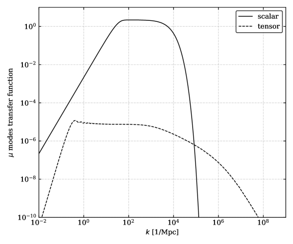
Figure 1: Plot of the $\mu$ modes transfer function for scalar and tensor perturbations.

Fig. 1 shows that tensor perturbations contribute to the generation of $\mu$-distortions over a vast range of scales, $k\simeq 1-10^{6}\,\mbox{Mpc}^{-1}$, and have a power-law decay for contributions $k>10^{6}\,\mbox{Mpc}^{-1}$. In contrast, the dissipation of scalar perturbations is limited to scales $k\simeq 50-10^{4}\,\mbox{Mpc}^{-1}$, with a strong exponential decay for contributions $k>10^{4}\,\mbox{Mpc}^{-1}$. The peak of the scalar transfer function is about five orders of magnitude greater than that of the tensor transfer function. These differences in the $\mu$-transfer functions arise because perturbations in the photon fluid sourced by primordial perturbations dissipate their energy differently. In general, perturbations in the photon fluid dissipate through photon-electron scattering and free-streaming effects. However, tensor perturbations dissipate only through free-streaming effects, and so the dissipation cuts off as a power law as rather than an exponential as is the case for scalar modes. Consequently, dissipation of the photon fluid perturbations sourced by tensor perturbations extends over a larger range of scales. Moreover, as transverse, traceless perturbations, tensor perturbations are not significantly attenuated by the CMB photon fluid (as is the case of longitudinal scalar perturbations), hence the tensor dissipation rate is suppressed relative to scalar dissipation. That is, the heat injection is much more inefficient in the case of tensor perturbations, leading to five orders of magnitude difference observed in fig. 1.

By removing the expectation value from eq. (2.43), we can write down its explicit connection to primordial perturbations as

$$\mu^{\rm primord,s}(\vec{x})=\int\frac{d^{3}\vec{k}_{1}\,d^{3}\vec{k}_{2}}{(2\pi)^{6}}\,\zeta(\vec{k}_{1})\,\zeta(\vec{k}_{2})\,\sqrt{W_{\zeta}\left(k_{1}\right)}\sqrt{W_{\zeta}\left(k_{2}\right)}\,e^{i\vec{k}_{+}\cdot\vec{x}}$$ (2.55)

for scalar perturbations and

$$\mu^{\rm primord,t}(\vec{x})=\int\frac{d^{3}\vec{k}_{1}\,d^{3}\vec{k}_{2}}{(2\pi)^{6}}\,\gamma_{ij}(\vec{k}_{1})\,\gamma^{ij}(\vec{k}_{2})\,\sqrt{W_{t}\left(k_{1}\right)}\sqrt{W_{t}\left(k_{2}\right)}\,e^{i\vec{k}_{+}\cdot\vec{x}}$$ (2.56)

for tensor perturbations, where $\vec{k}_{+}=\vec{k}_{1}+\vec{k}_{2}$ and $\vec{x}$ is the position on the last scattering surface.

As we have done with the CMB $T$, $E$ and $B$ modes, we can make an angular expansion of eqs. (2.55) and (2.56) in spherical harmonics as

$$a_{\ell m}^{\mu}=\int d\hat{x}\,Y^{*}_{\ell m}(\hat{x})\,\mu^{\rm primord}(\vec{x})~{},$$ (2.57)

which for scalar and tensor perturbations becomes respectively

$$a_{\ell m}^{\mu,s}=4\pi\,(-i)^{\ell}\,\int\frac{d^{3}\vec{k}_{1}\,d^{3}\vec{k}_{2}}{(2\pi)^{6}}\,Y^{*}_{\ell m}(\hat{k}_{+})\,\zeta(\vec{k}_{1})\,\zeta(\vec{k}_{2})\,\sqrt{W_{\zeta}\left(k_{1}\right)}\sqrt{W_{\zeta}\left(k_{2}\right)}\,j_{\ell}(k_{+}r_{L})$$ (2.58)

and

$$a_{\ell m}^{\mu,t}=4\pi\,(-i)^{\ell}\,\int\frac{d^{3}\vec{k}_{1}\,d^{3}\vec{k}_{2}}{(2\pi)^{6}}\,Y^{*}_{\ell m}(\hat{k}_{+})\,\gamma_{ij}(\vec{k}_{1})\,\gamma^{ij}(\vec{k}_{2})\,\sqrt{W_{t}\left(k_{1}\right)}\sqrt{W_{t}\left(k_{2}\right)}\,j_{\ell}(k_{+}r_{L})\,.$$ (2.59)

Here, $r_{L}\simeq 1.4\times 10^{4}\,\mbox{Mpc}$ is the distance to the last scattering surface and we have made use of the following identities

$$e^{i\vec{k}\cdot\vec{x}}=\sum_{\ell}(2\ell+1)i^{\ell}P_{\ell}(\hat{k}\cdot\hat{x})\,j_{\ell}(kx)\,,$$ (2.60)

and

$$P_{\ell}(\hat{k}\cdot\hat{x})=\frac{4\pi}{2\ell+1}\sum_{m}\,Y_{\ell m}(\hat{k})\,Y^{*}_{\ell m}(\hat{x})\,.$$ (2.61)

Using the conventions and the results summarized in this section, we proceed in the next section to compute all possible cross-correlations between CMB $\mu$-spectral distortions (which we henceforth refer to as "SD") and CMB $T$, $E$ and $B$ anisotropies (henceforth referred to as "CMB").

3 Non-Gaussianities from SD-CMB cross-correlations

3.1 Definition of SD-CMB cross-correlations

We start this section by defining the following $\langle\mu X\rangle$ angular cross-correlation

$$C^{\mu X}_{\ell_{1}\ell_{2}m_{1}m_{2}}=\langle a_{\ell_{1}m_{1}}^{\mu}\,a_{\ell_{2}m_{2}}^{X*}\rangle\,,$$ (3.1)

where $X=T,E,B$.

Note that, by construction, eq. (3.1) is sensitive to primordial NGs, since it is proportional to the expectation value of the products of three (primordial) fields. In [38, 98, 97, 99, 43] the effects of pure scalar NGs in the $\langle\mu T\rangle$ and $\langle\mu E\rangle$ cross-correlations were considered. As emphasized in these references, SD-CMB cross-correlations are sensitive to the squeezed limit of the scalar bispectrum. The physical reason behind this is that, even if we cross-correlate CMB anisotropies and $\mu$-distortions at the same angular scales, the primordial perturbations that seeded them refer to very different scales. In particular, $\mu$-distortions are generated by primordial perturbations evaluated at scales much smaller than CMB temperature and polarization anisotropies . Schematically, in the cross-correlations of the type (3.1) $\mu$-distortions and a CMB anisotropies mode $X$ take non-negligible contributions by short and long modes respectively, as

$$\mu\propto\zeta_{\vec{k}_{s}}\,\zeta_{-\vec{k}_{s}},\,\,\gamma_{\vec{k}_{s}}\,\gamma_{-\vec{k}_{s}}\qquad\qquad T,E\propto\zeta_{\vec{k}_{l}},\,\,\gamma_{\vec{k}_{l}}\qquad\qquad B\propto\gamma_{\vec{k}_{l}}\,,$$ (3.2)

where we have assumed that CMB $B$ modes are sourced by tensor perturbations only (on large scales).

In the following, we show an original computation of the effects of statistical anisotropies in primordial NGs defined in sec. 2.2 on the cross-correlations of the type (3.1). In fact the presence of arbitrary breakings of statistical isotropy in our primordial correlators as evident in eqs. (2.19)-(2.22) is something new with respect to previous analyses.

3.2 $\langle\mu T\rangle$

Here, we focus on the $\langle\mu T\rangle$ (angular) cross-correlation. Mathematically this reads

$$C^{\mu T}_{\ell_{1}\ell_{2}m_{1}m_{2}}=\langle a_{\ell_{1}m_{1}}^{\mu}\,a_{\ell_{2}m_{2}}^{T*}\rangle\,.$$ (3.3)

By considering the scheme in eq. (3.2) this cross-correlation is affected by all the types of primordial bispectra considered in sec. 2.2, i.e. schematically

$$C^{\mu T}_{\ell_{1}\ell_{2}m_{1}m_{2}}\propto\langle\zeta_{\vec{k}_{s}}\zeta_{-\vec{k}_{s}}\zeta_{\vec{k}_{l}}\rangle,\langle\gamma_{\vec{k}_{s}}\gamma_{-\vec{k}_{s}}\zeta_{\vec{k}_{l}}\rangle,\langle\gamma_{\vec{k}_{s}}\gamma_{-\vec{k}_{s}}\gamma_{\vec{k}_{l}}\rangle,\langle\zeta_{\vec{k}_{s}}\zeta_{-\vec{k}_{s}}\gamma_{\vec{k}_{l}}\rangle\,.$$ (3.4)

In the following, we compute all these contributions separately.

3-scalars contribution

The contributions from the 3-scalars primordial bispectrum is given by substituting eqs. (2.39) and (2.58) into (3.3). We get

$$C^{\mu T}_{\ell_{1}\ell_{2}m_{1}m_{2}}= i^{\ell_{2}-\ell_{1}}\,16\pi^{2}\int\frac{d^{3}k\,d^{3}k_{1}\,d^{3}k_{2}}{(2\pi)^{9}}{\cal T}_{\ell_{2}(s)}^{T}(k)\,j_{\ell_{1}}(k_{+}r_{L})\,\sqrt{W_{\zeta}\left(k_{1}\right)}\,\sqrt{W_{\zeta}\left(k_{2}\right)}$$

$$\qquad\qquad\qquad\qquad\qquad\qquad\times Y_{\ell_{1}m_{1}}^{*}(\hat{k}_{+})\,Y_{\ell_{2}m_{2}}(\hat{k})\left[\braket{\zeta_{\vec{k}_{1}}\zeta_{\vec{k}_{2}}\zeta_{-\vec{k}}}\right]\,.$$ (3.5)

We can integrate one of the three momenta by employing the Dirac delta in the definition of primordial bispectra (2.1). We obtain

$$C^{\mu T}_{\ell_{1}\ell_{2}m_{1}m_{2}}= i^{\ell_{2}-\ell_{1}}\,16\pi^{2}\int\frac{d^{3}k_{1}\,d^{3}k_{2}}{(2\pi)^{6}}\,{\cal T}_{\ell_{2}(s)}^{T}(k_{+})\,j_{\ell_{1}}(k_{+}r_{L})\,\sqrt{W_{\zeta}\left(k_{1}\right)}\,\sqrt{W_{\zeta}\left(k_{2}\right)}$$

$$\qquad\qquad\qquad\qquad\qquad\qquad\times Y_{\ell_{1}m_{1}}^{*}(\hat{k}_{+})\,Y_{\ell_{2}m_{2}}(\hat{k}_{+})\left[B_{\zeta\zeta\zeta}(\vec{k}_{1},\vec{k}_{2},-\vec{k}_{+})\right]\,.$$ (3.6)

Note that it is much more convenient switching the momenta integrations from $\vec{k}_{1},\vec{k}_{2}$ to $\vec{k}_{+},\vec{k}_{-}$ by the change of variable $\vec{k}_{\pm}=\vec{k}_{1}\pm\vec{k}_{2}$. This leads to

$$C^{\mu T}_{\ell_{1}\ell_{2}m_{1}m_{2}}= i^{\ell_{2}-\ell_{1}}2\pi^{2}\int\frac{d^{3}k_{+}\,d^{3}k_{-}}{(2\pi)^{6}}\,{\cal T}_{\ell_{2}(s)}^{T}(k_{+})\,j_{\ell_{1}}(k_{+}r_{L})\,\sqrt{W_{\zeta}\left(|(\vec{k}_{+}+\vec{k}_{-})/2|\right)}$$

$$\qquad\qquad\qquad\qquad\qquad\times\,\sqrt{W_{\zeta}\left(|(\vec{k}_{+}-\vec{k}_{-})/2|\right)}\,Y_{\ell_{1}m_{1}}^{*}(\hat{k}_{+})\,Y_{\ell_{2}m_{2}}(\hat{k}_{+})$$

$$\qquad\qquad\qquad\qquad\qquad\times\left[B_{\zeta\zeta\zeta}((\vec{k}_{+}+\vec{k}_{-})/2,(\vec{k}_{+}-\vec{k}_{-})/2,-\vec{k}_{+})\right]\,.$$ (3.7)

Due to the simultaneous presence of the SD and CMB transfer functions, the integration over $\vec{k}_{+}$ and $\vec{k}_{-}$ gives a non-negligible contribution only on the very squeezed configurations where $\vec{k}_{+}\rightarrow 0$, i.e. when a scalar wavelength-mode is much greater than the other two scalar modes.

By substituting the squeezed bispectrum (2.19) into (3.2), we get

$$C^{\mu T}_{\ell_{1}\ell_{2}m_{1}m_{2}}= i^{\ell_{2}-\ell_{1}}\,64\pi^{3}\,\int\frac{dk_{+}\,dk_{-}}{(2\pi)^{6}}\,k_{+}^{2}\,k_{-}^{2}\,{\cal T}_{\ell_{2}(s)}^{T}(k_{+})\,j_{\ell_{1}}(k_{+}r_{L})\,W_{\zeta}\left(k_{-}\right)P_{\zeta}(k_{-})P_{\zeta}(k_{+})$$

$$\times\,\left[\sum_{L_{1},M_{1}}\sum_{L_{2},M_{2}}f_{L_{1},M_{1},L_{2},M_{2}}^{\rm sss}\,\int d\hat{k}_{-}\,Y_{L_{2}M_{2}}(\hat{k}_{-})\,\int d\hat{k}_{+}\,Y_{L_{1}M_{1}}(-\hat{k}_{+})\,Y_{\ell_{2}m_{2}}(\hat{k}_{+})\,Y_{\ell_{1}m_{1}}^{*}(\hat{k}_{+})\right]\,,$$ (3.8)

where we have rescaled the momentum $k_{-}$ ($\vec{k}_{-}^{\prime}=\vec{k}_{-}/2$). Here, the angular integration over $\hat{k}_{-}$ is trivial as it is non-zero only if $L_{2}=M_{2}=0$, while the angular integration over $\hat{k}_{+}$ can be done in terms of Wigner 3-j symbols (see eq. (B) in app. B) and we get

$$C^{\mu T}_{\ell_{1}\ell_{2}m_{1}m_{2}}= i^{\ell_{2}-\ell_{1}}\,64\pi^{3}\int\frac{dk_{+}\,dk_{-}}{(2\pi)^{6}}\,k_{+}^{2}\,k_{-}^{2}\,{\cal T}_{\ell_{2}(s)}^{T}(k_{+})\,j_{\ell_{1}}(k_{+}r_{L})\,W_{\zeta}\left(k_{-}\right)P_{\zeta}(k_{-})P_{\zeta}(k_{+})$$

$$\times\left[\sum_{L_{1},M_{1}}\,f_{L_{1},M_{1}}^{\rm sss}\,(-1)^{m_{1}+L_{1}}\sqrt{(2\ell_{1}+1)(2\ell_{2}+1)(2L_{1}+1)}\,\begin{pmatrix}\ell_{1}&\ell_{2}&L_{1}\\ 0&0&0\end{pmatrix}\begin{pmatrix}\ell_{1}&\ell_{2}&L_{1}\\ -m_{1}&m_{2}&M_{1}\end{pmatrix}\right]\,,$$ (3.9)

where for brevity here and afterwards we will indicate $f_{L_{1},M_{1}}^{xxx}\equiv f_{L_{1},M_{1},0,0}^{xxx}$.

We can rewrite this equation in terms of dimensionless amplitudes as

$$C^{\mu T,\,\,\zeta\zeta\zeta}_{\ell_{1}\ell_{2}m_{1}m_{2}}= i^{\ell_{2}-\ell_{1}}\,\sum_{L_{1},M_{1}}\,(-1)^{m_{1}+L_{1}}\sqrt{(2\ell_{1}+1)(2\ell_{2}+1)(2L_{1}+1)}\,\begin{pmatrix}\ell_{1}&\ell_{2}&L_{1}\\ 0&0&0\end{pmatrix}\begin{pmatrix}\ell_{1}&\ell_{2}&L_{1}\\ -m_{1}&m_{2}&M_{1}\end{pmatrix}$$

$$\times\,4\pi\,\mathcal{I}^{\ell_{1}\ell_{2},L_{1}M_{1},T}_{\zeta\zeta\zeta}\,,$$ (3.10)

where we defined the integral

$$\mathcal{I}^{\ell_{1}\ell_{2},L_{1}M_{1},T}_{\zeta\zeta\zeta}=\int d\ln k_{+}\,d\ln k_{-}\,\,{\cal T}_{\ell_{2}(s)}^{T}(k_{+})\,j_{\ell_{1}}(k_{+}r_{L})\,W_{\zeta}\left(k_{-}\right)\,\mathcal{A}_{s}(k_{-})\,\mathcal{A}_{s}(k_{+})\,f_{L_{1},M_{1}}^{\rm sss}\,,$$ (3.11)

which is sensitive to the physical details of a given inflationary model.

1-scalar 2-tensors contribution

The contribution from the 1-scalar 2-tensors primordial bispectrum is obtained by substituting eqs. (2.39) and (2.59) into (3.3). We get

$$C^{\mu T}_{\ell_{1}\ell_{2}m_{1}m_{2}}= i^{\ell_{2}-\ell_{1}}\sum_{\lambda,\,\lambda^{\prime}}\,16\pi^{2}\int\frac{d^{3}k\,d^{3}k_{1}\,d^{3}k_{2}}{(2\pi)^{9}}{\cal T}_{\ell_{2}(s)}^{T}(k)\,j_{\ell_{1}}(k_{+}r_{L})Y_{\ell_{1}m_{1}}^{*}(\hat{k}_{+})$$

$$\qquad\qquad\qquad\qquad\qquad\qquad\qquad\times\epsilon_{ij}^{\lambda}(\vec{k}_{1})\epsilon^{ij,\lambda^{\prime}}(\vec{k}_{2})\,\sqrt{W_{t}\left(k_{1}\right)}\,\sqrt{W_{t}\left(k_{2}\right)}$$

$$\qquad\qquad\qquad\qquad\qquad\qquad\qquad\times Y_{\ell_{2}m_{2}}(\hat{k})\left[\braket{\gamma^{\lambda}_{\vec{k}_{1}}\gamma^{\lambda^{\prime}}_{\vec{k}_{2}}\zeta_{-\vec{k}}}\right]\,.$$ (3.12)

As before, we can integrate out one of the three momenta, employing the Dirac delta in the definition of the primordial bispectra and switching to the momenta $\vec{k}_{+},\vec{k}_{-}$. We obtain

$$C^{\mu T}_{\ell_{1}\ell_{2}m_{1}m_{2}}= i^{\ell_{2}-\ell_{1}}\sum_{\lambda,\,\lambda^{\prime}}2\pi^{2}\int\frac{d^{3}k_{+}\,d^{3}k_{-}}{(2\pi)^{6}}\,{\cal T}_{\ell_{2}(s)}^{T}(k_{+})\,j_{\ell_{1}}(k_{+}r_{L})$$

$$\qquad\qquad\qquad\qquad\times\sqrt{W_{t}\left(|(\vec{k}_{+}+\vec{k}_{-})/2|\right)}\sqrt{W_{t}\left(|(\vec{k}_{+}-\vec{k}_{-})/2|\right)}$$

$$\qquad\qquad\qquad\qquad\times\epsilon_{ij}^{\lambda}\left((\vec{k}_{+}+\vec{k}_{-})/2\right)\,\epsilon^{ij,\lambda^{\prime}}\left((\vec{k}_{+}-\vec{k}_{-})/2\right)\,Y_{\ell_{1}m_{1}}^{*}(\hat{k}_{+})\,Y_{\ell_{2}m_{2}}(\hat{k}_{+})$$

$$\qquad\qquad\qquad\qquad\qquad\times\left[B^{\lambda\lambda^{\prime}}((\vec{k}_{+}+\vec{k}_{-})/2,(\vec{k}_{+}-\vec{k}_{-})/2,-\vec{k}_{+})\right]\,.$$ (3.13)

Again, the integration over the momenta gives a non-negligible contribution only in the squeezed configurations when the scalar wavelength-mode is much greater than the two tensor modes.

By substituting the squeezed bispectrum (2.21) in eq. (3.2), and expressing the angular integrations in terms of the Wigner 3-j symbols as above, we get the final result

$$C^{\mu T}_{\ell_{1}\ell_{2}m_{1}m_{2}}= i^{\ell_{2}-\ell_{1}}\,128\pi^{3}\int\frac{dk_{+}\,dk_{-}}{(2\pi)^{6}}\,k_{+}^{2}\,k_{-}^{2}\,{\cal T}_{\ell_{2}(s)}^{T}(k_{+})\,j_{\ell_{1}}(k_{+}r_{L})\,W_{\zeta}\left(k_{-}\right)P_{t}(k_{-})P_{\zeta}(k_{+})$$

$$\times\left[\sum_{L_{1},M_{1}}\,f_{L_{1},M_{1}}^{\rm stt}\,(-1)^{m_{1}+L_{1}}\sqrt{(2\ell_{1}+1)(2\ell_{2}+1)(2L_{1}+1)}\,\begin{pmatrix}\ell_{1}&\ell_{2}&L_{1}\\ 0&0&0\end{pmatrix}\begin{pmatrix}\ell_{1}&\ell_{2}&L_{1}\\ -m_{1}&m_{2}&M_{1}\end{pmatrix}\right]$$

$$\times\left(\sum_{\lambda,\,\lambda^{\prime}}\xi_{\lambda\lambda^{\prime}}\right)\,.$$ (3.14)

We can express this result in terms of dimensionless amplitudes as

$$C^{\mu T,\,\,\gamma\gamma\zeta}_{\ell_{1}\ell_{2}m_{1}m_{2}}= \sum_{L_{1},M_{1}}\,(-1)^{m_{1}+L_{1}}\sqrt{(2\ell_{1}+1)(2\ell_{2}+1)(2L_{1}+1)}\,\begin{pmatrix}\ell_{1}&\ell_{2}&L_{1}\\ 0&0&0\end{pmatrix}\begin{pmatrix}\ell_{1}&\ell_{2}&L_{1}\\ -m_{1}&m_{2}&M_{1}\end{pmatrix}$$

$$\times\,8\pi\,\left(\sum_{\lambda,\,\lambda^{\prime}}\xi_{\lambda\lambda^{\prime}}\right)\,\mathcal{I}^{\ell_{1}\ell_{2},L_{1}M_{1},T}_{\gamma\gamma\zeta}\,,$$ (3.15)

where

$$\mathcal{I}^{\ell_{1}\ell_{2},L_{1}M_{1},T}_{\gamma\gamma\zeta}=\int d\ln k_{+}\,d\ln k_{-}\,\,{\cal T}_{\ell_{2}(s)}^{T}(k_{+})\,j_{\ell_{1}}(k_{+}r_{L})\,W_{t}\left(k_{-}\right)\,\mathcal{A}_{t}(k_{-})\,\mathcal{A}_{s}(k_{+})\,f_{L_{1},M_{1}}^{\rm stt}\,.$$ (3.16)

2-scalars 1-tensor contribution

The contribution from the 2-scalars 1-tensor primordial bispectrum is found by substituting eqs. (2.40) and (2.58) into (3.3). We get

$$C^{\mu T}_{\ell_{1}\ell_{2}m_{1}m_{2}}= i^{\ell_{2}-\ell_{1}}\,16\pi^{2}\int\frac{d^{3}k\,d^{3}k_{1}\,d^{3}k_{2}}{(2\pi)^{9}}{\cal T}_{\ell_{2}(t)}^{T}(k)\,j_{\ell_{1}}(k_{+}r_{L})\,\sqrt{W_{\zeta}\left(k_{1}\right)}\,\sqrt{W_{\zeta}\left(k_{2}\right)}$$

$$\qquad\qquad\qquad\quad\times Y_{\ell_{1}m_{1}}^{*}(\hat{k}_{+})\,\left[{}_{-2}Y_{\ell_{2}m_{2}}(\hat{k})\braket{\zeta_{\vec{k}_{1}}\zeta_{\vec{k}_{2}}\gamma_{-\vec{k}}^{L}}+{}_{+2}Y_{\ell_{2}m_{2}}(\hat{k})\braket{\zeta_{\vec{k}_{1}}\zeta_{\vec{k}_{2}}\gamma_{-\vec{k}}^{R}}\right]\,.$$ (3.17)

By integrating out one of the three momenta by employing the Dirac delta in the definition of the primordial bispectra and going through the same steps as above we arrive at

$$C^{\mu T}_{\ell_{1}\ell_{2}m_{1}m_{2}}= i^{\ell_{2}-\ell_{1}}\,2\pi^{2}\int\frac{d^{3}k_{+}\,d^{3}k_{-}}{(2\pi)^{6}}\,{\cal T}_{\ell_{2}(t)}^{T}(k_{+})\,j_{\ell_{1}}(k_{+}r_{L})$$

$$\qquad\qquad\qquad\times\sqrt{W_{\zeta}\left(|(\vec{k}_{+}+\vec{k}_{-})/2|\right)}\,\sqrt{W_{\zeta}\left(|(\vec{k}_{+}-\vec{k}_{-})/2|\right)}$$

$$\qquad\qquad\qquad\times Y_{\ell_{1}m_{1}}^{*}(\hat{k}_{+})\,\left[{}_{-2}Y_{\ell_{2}m_{2}}(\hat{k}_{+})B^{L}((\vec{k}_{+}+\vec{k}_{-})/2,(\vec{k}_{+}-\vec{k}_{-})/2,-\vec{k}_{+})\right.$$

$$\qquad\qquad\qquad\qquad\qquad\qquad\qquad\left.+{}_{+2}Y_{\ell_{2}m_{2}}(\hat{k}_{+})B^{R}((\vec{k}_{+}+\vec{k}_{-})/2,(\vec{k}_{+}-\vec{k}_{-})/2,-\vec{k}_{+})\right]\,.$$ (3.18)

By substituting the squeezed bispectrum (2.20) into (3.2), we can rewrite this as

$$C^{\mu T}_{\ell_{1}\ell_{2}m_{1}m_{2}}= i^{\ell_{2}-\ell_{1}}\,64\pi^{3}\int\frac{dk_{+}\,dk_{-}}{(2\pi)^{6}}\,k_{+}^{2}\,k_{-}^{2}\,{\cal T}_{\ell_{2}(t)}^{T}(k_{+})\,j_{\ell_{1}}(k_{+}r_{L})\,W_{\zeta}\left(k_{-}\right)P_{\zeta}(k_{-})P_{t}(k_{+})$$

$$\qquad\qquad\times\sum_{L_{1},M_{1}}\sum_{L_{2},M_{2}}\,f_{L_{1},M_{1},L_{2},M_{2}}^{\rm sst}\int d\hat{k}_{-}\,Y_{L_{2}M_{2}}(\hat{k}_{-})$$

$$\qquad\qquad\times\int d\hat{k}_{+}\left[\xi_{L}\,\,{}_{+2}Y_{L_{1}M_{1}}(-\hat{k}_{+})\,{}_{-2}Y_{\ell_{2}m_{2}}(\hat{k}_{+})\,Y_{\ell_{1}m_{1}}^{*}(\hat{k}_{+})\right.$$

$$\left.\qquad\qquad\qquad\qquad\qquad\qquad+\xi_{R}\,\,{}_{-2}Y_{L_{1}M_{1}}(-\hat{k}_{+})\,{}_{+2}Y_{\ell_{2}m_{2}}(\hat{k}_{+})\,Y_{\ell_{1}m_{1}}^{*}(\hat{k}_{+})\right]\,.$$ (3.19)

As before, we now express the angular integrations in terms of Wigner 3-j symbols

$$C^{\mu T}_{\ell_{1}\ell_{2}m_{1}m_{2}}= i^{\ell_{2}-\ell_{1}}\,64\pi^{3}\int\frac{dk_{+}\,dk_{-}}{(2\pi)^{6}}\,k_{+}^{2}\,k_{-}^{2}\,{\cal T}_{\ell_{2}(t)}^{T}(k_{+})\,j_{\ell_{1}}(k_{+}r_{L})\,W_{\zeta}\left(k_{-}\right)P_{\zeta}(k_{-})P_{t}(k_{+})$$

$$\times\,\sum_{L_{1},M_{1}}\,(-1)^{m_{1}+L_{1}}\,f_{L_{1},M_{1}}^{\rm sst}\sqrt{(2\ell_{1}+1)(2\ell_{2}+1)(2L_{1}+1)}\,\begin{pmatrix}\ell_{1}&\ell_{2}&L_{1}\\ 0&2&-2\end{pmatrix}\begin{pmatrix}\ell_{1}&\ell_{2}&L_{1}\\ -m_{1}&m_{2}&M_{1}\end{pmatrix}$$

$$\times\left[\xi_{L}+(-1)^{\ell_{1}+\ell_{2}+L_{1}}\,\xi_{R}\right]\,.$$ (3.20)

We can express the final result in terms of dimensionless amplitudes as

$$C^{\mu T,\,\,\zeta\zeta\gamma}_{\ell_{1}\ell_{2}m_{1}m_{2}}= i^{\ell_{2}-\ell_{1}}\,\sum_{L_{1},M_{1}}\,(-1)^{m_{1}+L_{1}}\,\sqrt{(2\ell_{1}+1)(2\ell_{2}+1)(2L_{1}+1)}\,\begin{pmatrix}\ell_{1}&\ell_{2}&L_{1}\\ 0&2&-2\end{pmatrix}\begin{pmatrix}\ell_{1}&\ell_{2}&L_{1}\\ -m_{1}&m_{2}&M_{1}\end{pmatrix}$$

$$\times\,4\pi\,\mathcal{I}^{\ell_{1}\ell_{2},L_{1}M_{1},T}_{\zeta\zeta\gamma}\,,$$ (3.21)

where

$$\mathcal{I}^{\ell_{1}\ell_{2},L_{1}M_{1},T}_{\zeta\zeta\gamma}=\int d\ln k_{+}\,d\`{\i}\ln k_{-}\, {\cal T}_{\ell_{2}(t)}^{T}(k_{+})\,j_{\ell_{1}}(k_{+}r_{L})\,W_{\zeta}\left(k_{-}\right)\,\mathcal{A}_{s}(k_{-})\,\mathcal{A}_{t}(k_{+})\,f_{L_{1},M_{1}}^{\rm sst}$$

$$\times\left[\xi_{L}+(-1)^{\ell_{1}+\ell_{2}+L_{1}}\,\xi_{R}\right]\,.$$ (3.22)

3-tensors contribution

The contribution from the 3-tensors primordial bispectrum is given by substituting eqs. (2.40) and (2.59) into (3.3). We get

$$C^{\mu T}_{\ell_{1}\ell_{2}m_{1}m_{2}}= i^{\ell_{2}-\ell_{1}}\,\sum_{\lambda,\,\lambda^{\prime}}\,16\pi^{2}\int\frac{d^{3}k\,d^{3}k_{1}\,d^{3}k_{2}}{(2\pi)^{9}}{\cal T}_{\ell_{2}(t)}^{T}(k)\,j_{\ell_{1}}(k_{+}r_{L})\,Y_{\ell_{1}m_{1}}^{*}(\hat{k}_{+})$$

$$\qquad\qquad\qquad\qquad\qquad\times\,\epsilon_{ij}^{\lambda}(\vec{k}_{1})\epsilon^{ij,\lambda^{\prime}}(\vec{k}_{2})\,\sqrt{W_{t}\left(k_{1}\right)}\sqrt{W_{t}\left(k_{2}\right)}\,$$

$$\qquad\qquad\qquad\qquad\qquad\times\left[{}_{-2}Y_{\ell_{2}m_{2}}(\hat{k})\braket{\mathcal{\gamma}^{\lambda}_{\vec{k_{1}}}\mathcal{\gamma}^{\lambda^{\prime}}_{\vec{k_{2}}}\gamma_{-\vec{k}}^{L}}+{}_{+2}Y_{\ell_{2}m_{2}}(\hat{k})\braket{\mathcal{\gamma}^{\lambda}_{\vec{k_{1}}}\mathcal{\gamma}^{\lambda^{\prime}}_{\vec{k_{2}}}\gamma_{-\vec{k}}^{R}}\right]\,.$$ (3.23)

By going through steps analogous to above we arrive at

$$C^{\mu T}_{\ell_{1}\ell_{2}m_{1}m_{2}}= i^{\ell_{2}-\ell_{1}}\,\sum_{\lambda,\,\lambda^{\prime}}\,2\pi^{2}\int\frac{d^{3}k_{+}\,d^{3}k_{-}}{(2\pi)^{6}}\,{\cal T}_{\ell_{2}(t)}^{T}(k_{+})\,j_{\ell_{1}}(k_{+}r_{L})\,\epsilon_{ij}^{\lambda}\left((\vec{k}_{+}+\vec{k}_{-})/2\right)$$

$$\qquad\qquad\qquad\times\,\epsilon^{ij,\lambda^{\prime}}\left((\vec{k}_{+}-\vec{k}_{-})/2\right)\sqrt{W_{t}\left(|(\vec{k}_{+}+\vec{k}_{-})/2|\right)}\sqrt{W_{t}\left(|(\vec{k}_{+}-\vec{k}_{-})/2|\right)}$$

$$\qquad\qquad\qquad\times Y_{\ell_{1}m_{1}}^{*}(\hat{k}_{+})\,\left[{}_{-2}Y_{\ell_{2}m_{2}}(\hat{k}_{+})B^{\lambda\lambda^{\prime}L}((\vec{k}_{+}+\vec{k}_{-})/2,(\vec{k}_{+}-\vec{k}_{-})/2,-\vec{k}_{+})\right.$$

$$\qquad\qquad\qquad\qquad\qquad\qquad\left.+{}_{+2}Y_{\ell_{2}m_{2}}(\hat{k}_{+})B^{\lambda\lambda^{\prime}R}((\vec{k}_{+}+\vec{k}_{-})/2,(\vec{k}_{+}-\vec{k}_{-})/2,-\vec{k}_{+})\right]\,.$$ (3.24)

By substituting the squeezed bispectrum (2.22) into (3.2), we find

$$C^{\mu T}_{\ell_{1}\ell_{2}m_{1}m_{2}}= i^{\ell_{2}-\ell_{1}}\,128\pi^{3}\int\frac{dk_{+}\,dk_{-}}{(2\pi)^{6}}\,k_{+}^{2}\,k_{-}^{2}\,{\cal T}_{\ell_{2}(t)}^{T}(k_{+})\,W_{t}\left(k_{-}\right)\,j_{\ell_{1}}(k_{+}r_{L})\,P_{t}(k_{+})P_{t}(k_{-})$$

$$\qquad\qquad\times\,\sum_{L_{1},M_{1}}\sum_{L_{2},M_{2}}\,f_{L_{1},M_{1},L_{2},M_{2}}^{\rm sst}\,\int d\hat{k}_{-}\,Y_{L_{2}M_{2}}(\hat{k}_{-})$$

$$\qquad\qquad\times\,\int d\hat{k}_{+}\,\left[(\xi_{LLL}+\xi_{LLR})\,{}_{+2}Y_{L_{1}M_{1}}(-\hat{k}_{+})\,{}_{-2}Y_{\ell_{2}m_{2}}(\hat{k}_{+})\,Y_{\ell_{1}m_{1}}^{*}(\hat{k}_{+})\right.$$

$$\left.\qquad\qquad\qquad\qquad\qquad\qquad+(\xi_{RRL}+\xi_{RRR})\,{}_{-2}Y_{L_{1}M_{1}}(-\hat{k}_{+})\,{}_{+2}Y_{\ell_{2}m_{2}}(\hat{k}_{+})\,Y_{\ell_{1}m_{1}}^{*}(\hat{k}_{+})\right]\,.$$ (3.25)

The angular integrations are expressed in terms of Wigner 3-j symbols as above and we obtain the final result

$$C^{\mu T,\,\,\gamma\gamma\gamma}_{\ell_{1}\ell_{2}m_{1}m_{2}}= i^{\ell_{2}-\ell_{1}}\,\sum_{L_{1},M_{1}}\,(-1)^{m_{1}+L_{1}}\,\sqrt{(2\ell_{1}+1)(2\ell_{2}+1)(2L_{1}+1)}\,\begin{pmatrix}\ell_{1}&\ell_{2}&L_{1}\\ 0&2&-2\end{pmatrix}\begin{pmatrix}\ell_{1}&\ell_{2}&L_{1}\\ -m_{1}&m_{2}&M_{1}\end{pmatrix}$$

$$\times\,8\pi\,\mathcal{I}^{\ell_{1}\ell_{2},L_{1}M_{1},T}_{\gamma\gamma\gamma}\,,$$ (3.26)

where

$$\mathcal{I}^{\ell_{1}\ell_{2},L_{1}M_{1},T}_{\gamma\gamma\gamma}=\int d\ln k_{+}\,d\ln k_{-}\, {\cal T}_{\ell_{2}(t)}^{T}(k_{+})\,j_{\ell_{1}}(k_{+}r_{L})\,W_{t}\left(k_{-}\right)\,\mathcal{A}_{t}(k_{+})\,\mathcal{A}_{t}(k_{-})\,f_{L_{1},M_{1}}^{\rm ttt}$$

$$\times\left[(\xi_{LLL}+\xi_{LLR})+(-1)^{\ell_{1}+\ell_{2}+L_{1}}\,(\xi_{RRL}+\xi_{RRR})\right]\,.$$ (3.27)

3.3 $\langle\mu E\rangle$

Here, we focus on the $\langle\mu E\rangle$ (angular) cross-correlation defined as

$$C^{\mu E}_{\ell_{1}\ell_{2}m_{1}m_{2}}=\langle a_{\ell_{1}m_{1}}^{\mu}\,a_{\ell_{2}m_{2}}^{E*}\rangle\,.$$ (3.28)

The computations resemble the $\langle\mu T\rangle$ case, apart for the substitution $T\rightarrow E$. Therefore, in the following we show only the final results.

3-scalars contribution

$$C^{\mu E,\,\,\zeta\zeta\zeta}_{\ell_{1}\ell_{2}m_{1}m_{2}}= \sum_{L_{1},M_{1}}\,(-1)^{m_{1}+L_{1}}\sqrt{(2\ell_{1}+1)(2\ell_{2}+1)(2L_{1}+1)}\,\begin{pmatrix}\ell_{1}&\ell_{2}&L_{1}\\ 0&0&0\end{pmatrix}\begin{pmatrix}\ell_{1}&\ell_{2}&L_{1}\\ -m_{1}&m_{2}&M_{1}\end{pmatrix}$$

$$\times\,4\pi\,\mathcal{I}^{\ell_{1}\ell_{2},L_{1}M_{1},E}_{\zeta\zeta\zeta}\,,$$ (3.29)

where

$$\mathcal{I}^{\ell_{1}\ell_{2},L_{1}M_{1},E}_{\zeta\zeta\zeta}=\int d\ln k_{+}\,d\ln k_{-}\,\,{\cal T}_{\ell_{2}(s)}^{E}(k_{+})\,j_{\ell_{1}}(k_{+}r_{L})\,W_{s}\left(k_{-}\right)\,\mathcal{A}_{s}(k_{-})\,\mathcal{A}_{s}(k_{+})\,f_{L_{1},M_{1}}^{\rm sss}\,.$$ (3.30)

1-scalar 2-tensors contribution

$$C^{\mu E,\,\,\gamma\gamma\zeta}_{\ell_{1}\ell_{2}m_{1}m_{2}}= \sum_{L_{1},M_{1}}\,(-1)^{m_{1}+L_{1}}\sqrt{(2\ell_{1}+1)(2\ell_{2}+1)(2L_{1}+1)}\,\begin{pmatrix}\ell_{1}&\ell_{2}&L_{1}\\ 0&0&0\end{pmatrix}\begin{pmatrix}\ell_{1}&\ell_{2}&L_{1}\\ -m_{1}&m_{2}&M_{1}\end{pmatrix}$$

$$\times\,8\pi\,\left(\sum_{\lambda,\,\lambda^{\prime}}\xi_{\lambda\lambda^{\prime}}\right)\,\mathcal{I}^{\ell_{1}\ell_{2},L_{1}M_{1},E}_{\gamma\gamma\zeta}\,,$$ (3.31)

where

$$\mathcal{I}^{\ell_{1}\ell_{2},L_{1}M_{1},E}_{\gamma\gamma\zeta}=\int d\ln k_{+}\,d\ln k_{-}\,\,{\cal T}_{\ell_{2}(s)}^{E}(k_{+})\,j_{\ell_{1}}(k_{+}r_{L})\,W_{t}\left(k_{-}\right)\,\mathcal{A}_{t}(k_{-})\,\mathcal{A}_{s}(k_{+})\,f_{L_{1},M_{1}}^{\rm stt}\,.$$ (3.32)

2-scalars 1-tensor contribution

$$C^{\mu E,\,\,\zeta\zeta\gamma}_{\ell_{1}\ell_{2}m_{1}m_{2}}= i^{\ell_{2}-\ell_{1}}\,\sum_{L_{1},M_{1}}\,(-1)^{m_{1}+L_{1}}\,\sqrt{(2\ell_{1}+1)(2\ell_{2}+1)(2L_{1}+1)}\,\begin{pmatrix}\ell_{1}&\ell_{2}&L_{1}\\ 0&2&-2\end{pmatrix}\begin{pmatrix}\ell_{1}&\ell_{2}&L_{1}\\ -m_{1}&m_{2}&M_{1}\end{pmatrix}$$

$$\times\,4\pi\,\mathcal{I}^{\ell_{1}\ell_{2},L_{1}M_{1},E}_{\zeta\zeta\gamma}\,,$$ (3.33)

where

$$\mathcal{I}^{\ell_{1}\ell_{2},L_{1}M_{1},E}_{\zeta\zeta\gamma}=\int d\ln k_{+}\,d\ln k_{-}\, {\cal T}_{\ell_{2}(t)}^{E}(k_{+})\,j_{\ell_{1}}(k_{+}r_{L})\,W_{t}\left(k_{-}\right)\,\mathcal{A}_{t}(k_{+})\,\mathcal{A}_{s}(k_{-})\,f_{L_{1},M_{1}}^{\rm sst}$$

$$\times\left[\xi_{L}+(-1)^{\ell_{1}+\ell_{2}+L_{1}}\,\xi_{R}\right]\,.$$ (3.34)

3-tensors contribution

$$C^{\mu E,\,\,\gamma\gamma\gamma}_{\ell_{1}\ell_{2}m_{1}m_{2}}= i^{\ell_{2}-\ell_{1}}\,\sum_{L_{1},M_{1}}\,(-1)^{m_{1}+L_{1}}\,\sqrt{(2\ell_{1}+1)(2\ell_{2}+1)(2L_{1}+1)}\,\begin{pmatrix}\ell_{1}&\ell_{2}&L_{1}\\ 0&2&-2\end{pmatrix}\begin{pmatrix}\ell_{1}&\ell_{2}&L_{1}\\ -m_{1}&m_{2}&M_{1}\end{pmatrix}$$

$$\times\,8\pi\,\mathcal{I}^{\ell_{1}\ell_{2},L_{1}M_{1},E}_{\gamma\gamma\gamma}\,,$$ (3.35)

where

$$\mathcal{I}^{\ell_{1}\ell_{2},L_{1}M_{1},E}_{\gamma\gamma\gamma}=\int d\ln k_{+}\,d\ln k_{-}\, {\cal T}_{\ell_{2}(t)}^{E}(k_{+})\,j_{\ell_{1}}(k_{+}r_{L})\,W_{t}\left(k_{-}\right)\,\mathcal{A}_{t}(k_{+})\,\mathcal{A}_{t}(k_{-})\,f_{L_{1},M_{1}}^{\rm ttt}$$

$$\times\left[(\xi_{LLL}+\xi_{LLR})+(-1)^{\ell_{1}+\ell_{2}+L_{1}}\,(\xi_{RRL}+\xi_{RRR})\right]\,.$$ (3.36)

3.4 $\langle\mu B\rangle$

Here, we focus on the $\langle\mu B\rangle$ (angular) cross-correlation defined as

$$C^{\mu B}_{\ell_{1}\ell_{2}m_{1}m_{2}}=\langle a_{\ell_{1}m_{1}}^{\mu}\,a_{\ell_{2}m_{2}}^{(t)B*}\rangle\,.$$ (3.37)

Again, following the scheme (3.2), this cross-correlation will be proportional to the 1-graviton 2 scalars and 3-gravitons squeezed bispectra

$$C^{\mu B}_{\ell_{1}\ell_{2}m_{1}m_{2}}\propto\langle\zeta_{\vec{k}_{s}}\zeta_{-\vec{k}_{s}}\gamma_{\vec{k}_{l}}\rangle,\langle\gamma_{\vec{k}_{s}}\gamma_{-\vec{k}_{s}}\gamma_{\vec{k}_{l}}\rangle\,.$$ (3.38)

The computations resemble the $\langle\mu T\rangle$ case, apart for the exchange $T\rightarrow B$ and the sign flip $+\rightarrow-$ inside the square parenthesis in eqs. (3.2) and (3.2). Therefore, in the following we give only the final results.

2-scalars 1-tensor contribution

$$C^{\mu B,\,\,\zeta\zeta\gamma}_{\ell_{1}\ell_{2}m_{1}m_{2}}= i^{\ell_{2}-\ell_{1}}\,\sum_{L_{1},M_{1}}\,(-1)^{m_{1}+L_{1}}\,\sqrt{(2\ell_{1}+1)(2\ell_{2}+1)(2L_{1}+1)}\,\begin{pmatrix}\ell_{1}&\ell_{2}&L_{1}\\ 0&2&-2\end{pmatrix}\begin{pmatrix}\ell_{1}&\ell_{2}&L_{1}\\ -m_{1}&m_{2}&M_{1}\end{pmatrix}$$

$$\times\,4\pi\,\mathcal{I}^{\ell_{1}\ell_{2},L_{1}M_{1},B}_{\zeta\zeta\gamma}\,,$$ (3.39)

where

$$\mathcal{I}^{\ell_{1}\ell_{2},L_{1}M_{1},B}_{\zeta\zeta\gamma}=\int d\ln k_{+}\,d\ln k_{-}\, {\cal T}_{\ell_{2}(t)}^{B}(k_{+})\,j_{\ell_{1}}(k_{+}r_{L})\,W_{t}\left(k_{-}\right)\,\mathcal{A}_{t}(k_{+})\,\mathcal{A}_{s}(k_{-})\,f_{L_{1},M_{1}}^{\rm sst}$$

$$\times\left[\xi_{L}-(-1)^{\ell_{1}+\ell_{2}+L_{1}}\,\xi_{R}\right]\,.$$ (3.40)

3-tensors contribution

$$C^{\mu B,\,\,\gamma\gamma\gamma}_{\ell_{1}\ell_{2}m_{1}m_{2}}= i^{\ell_{2}-\ell_{1}}\,\sum_{L_{1},M_{1}}\,(-1)^{m_{1}+L_{1}}\,\sqrt{(2\ell_{1}+1)(2\ell_{2}+1)(2L_{1}+1)}\,\begin{pmatrix}\ell_{1}&\ell_{2}&L_{1}\\ 0&2&-2\end{pmatrix}\begin{pmatrix}\ell_{1}&\ell_{2}&L_{1}\\ -m_{1}&m_{2}&M_{1}\end{pmatrix}$$

$$\times\,8\pi\,\mathcal{I}^{\ell_{1}\ell_{2},L_{1}M_{1},B}_{\gamma\gamma\gamma}\,,$$ (3.41)

where

$$\mathcal{I}^{\ell_{1}\ell_{2},L_{1}M_{1},B}_{\gamma\gamma\gamma}=\int d\ln k_{+}\,d\ln k_{-}\, {\cal T}_{\ell_{2}(t)}^{B}(k_{+})\,j_{\ell_{1}}(k_{+}r_{L})\,W_{t}\left(k_{-}\right)\,\mathcal{A}_{t}(k_{+})\,\mathcal{A}_{t}(k_{-})\,f_{L_{1},M_{1}}^{\rm ttt}$$

$$\times\left[(\xi_{LLL}+\xi_{LLR})-(-1)^{\ell_{1}+\ell_{2}+L_{1}}\,(\xi_{RRL}+\xi_{RRR})\right]\,.$$ (3.42)

3.5 Comments

Let us make a few comments about these results. It turns out that $\langle\mu_{\ell_{1}}X_{\ell_{2}}\rangle$ angular cross-correlations may get $m$-dependent off-diagonal values ($\ell_{1}\neq\ell_{2}$) as a result of statistical anisotropies (induced by the long-mode $\hat{k}_{l}$ angular dependence) introduced in the squeezed primordial bispectra defined in sec. 2.2.

By virtue of the angular momentum algebra of the Wigner symbols, non-vanishing signals are limited to $|\ell_{1}-\ell_{2}|\leq L_{1}$. For analogous reasons, in cases where the long-wavelength mode is a tensor ($\langle\zeta\zeta\gamma\rangle$ and $\langle\gamma\gamma\gamma\rangle$), a non-zero signature requires $L_{1}\geq 2$. This means that by introducing the $\hat{k}_{l}$ dependence, we generate at least quadrupolar statistical anisotropies. Moreover, depending by the way in which primordial bispectra transform under parity transformation, only a given $\ell_{1}$, $\ell_{2}$ doublet can get a non-zero contribution. By applying the property of the Wigner symbols (B.3) we can easily verify the following identities

$$C^{\mu X,\,\,\zeta\zeta\zeta}_{\ell_{1}\ell_{2}m_{1}m_{2}}= (-1)^{\ell_{1}+\ell_{2}+L_{1}}\,C^{\mu X,\,\,\zeta\zeta\zeta}_{\ell_{1}\ell_{2}m_{1}m_{2}}\,,$$ (3.43)

$$C^{\mu X,\,\,\gamma\gamma\zeta}_{\ell_{1}\ell_{2}m_{1}m_{2}}= (-1)^{\ell_{1}+\ell_{2}+L_{1}}\,C^{\mu X,\,\,\gamma\gamma\zeta}_{\ell_{1}\ell_{2}m_{1}m_{2}}\,,$$ (3.44)

with $X=T,E$. Therefore, by collecting together what we found in this section and eq. (2.23), it is straightforward to realize that for the $\langle\zeta\zeta\zeta\rangle$ bispectrum and bispectra involving tensors with parity-even polarization coefficients we get a non-zero contribution in $\ell_{1},\ell_{2}$ doublets satisfying

$$\ell_{1}+\ell_{2}+L_{1}=\begin{cases}\mbox{even \qquad when }$X = E, T$\\ \mbox{odd \qquad when }$X = B$\,.\end{cases}$$ (3.45)

The same holds for the $\langle\gamma\gamma\zeta\rangle$ bispectrum with maximum violation of parity as described in eq. (2.25). Moreover, a $\langle\gamma\gamma\zeta\rangle$ bispectrum with parity-odd polarization coefficients would leave no signatures as $\sum_{\lambda\lambda^{\prime}}\xi_{\lambda\lambda^{\prime}}=0$. On the other hand, by eq. (2.24) it follows that for $\langle\zeta\zeta\gamma\rangle$ and $\langle\gamma\gamma\gamma\rangle$ bispectra with parity-odd polarization coefficents a non-zero signal is confined to

$$\ell_{1}+\ell_{2}+L_{1}=\begin{cases}\mbox{odd \qquad when }$X = E, T$\\ \mbox{even \qquad when }$X = B$\,.\end{cases}$$ (3.46)

Finally, no general conditions (apart for the constraint $|\ell_{1}-\ell_{2}|\leq L_{1}$) apply to $\langle\zeta\zeta\gamma\rangle$ and $\langle\gamma\gamma\gamma\rangle$ bispectra with maximum parity violation.

From our explicit calculations we note that the $\hat{k}_{-}(\equiv\hat{k}_{s})$ dependence in the angular integrations is always through the spin-0 spherical harmonics $Y_{L_{2}M_{2}}(\hat{k}_{-})$ only (see e.g. eq. (3.2)). Therefore, the resultant angular integration over $\hat{k}_{-}$ is always zero unless $L_{2}=0$, i.e. in absence of a $\hat{k}_{-}$ angular dependence. It follows that statistical anisotropies induced by the $\hat{k}_{s}$ dependence (and labelled by $L_{2}\neq 0$) get erased and do not contribute to SD-CMB cross-correlations. The physical interpretation of this comes from the physics of the spectral distortions: when we compute the $\mu$-distortion from the dissipation of acoustic-waves, we need to average the effect of primordial perturbations inside a spherical shell around the last scattering surface with a radius of order the dissipation scale at recombination (see, e.g., [38]). As a consequence, any $\hat{k}_{s}$ explicit angular dependence is averaged out to zero. For the same reason a $\hat{k}_{s}$ angular dependence induced by a long tensor mode in a rotationally invariant squeezed bispectrum is erased when averaging over this same spherical shell. Therefore, isotropic squeezed $\langle\gamma\zeta\zeta\rangle$ and $\langle\gamma\gamma\gamma\rangle$ bispectra leave no signatures to SD-CMB cross-correlations. This motivates a-posteriori our decision to study the statistically anisotropic case as we are mostly interested on signatures from bispectra involving tensor perturbations.

We end this section by noting that a similar less general discussion was first pointed out in [40], where the authors found that diagonal and off-diagonal $\langle\mu T\rangle$ cross-correlations with $|\ell_{1}-\ell_{2}|=2$ arise in scalar bispectra with a quadrupolar asymmetry (corresponding to our $\langle\zeta\zeta\zeta\rangle$, $L_{1}=2$, $L_{2}=0$ case).

In the next section, we aim to quantify the detectability prospects of the signatures studied in this section.

4 Forecasts

In this section, we make Fisher forecasts on the detectability of statistical anisotropies in primordial NGs with the cross-correlations we have computed in sec. 3. We will look into both parity preserving and parity violating patterns. As shown above, statistical anisotropies in squeezed bispectra could lead to off-diagonal elements in the SD-CMB cross-correlations $C^{\mu T}_{\ell_{1}\ell_{2}}$, $C^{\mu E}_{\ell_{1}\ell_{2}}$ and $C^{\mu B}_{\ell_{1}\ell_{2}}$.

Such statistical anisotropies are most effectively analyzed with the so-called BipoSH formalism [55, 56, 57]. Here we give a brief description of this formalism, referring to the original literature for more details. We begin by considering a generic cross-correlation in real space between two observables $\mathcal{O}^{1}$ and $\mathcal{O}^{2}$

$$\langle\mathcal{O}^{1}(\hat{x}_{1})\mathcal{O}^{2}(\hat{x}_{2})\rangle\,,$$ (4.1)

where $\hat{x}_{1}$ and $\hat{x}_{2}$ correspond to two different directions in the sky. We can expand this quantity as

$$\langle\mathcal{O}^{1}(\hat{x}_{1})\mathcal{O}^{2}(\hat{x}_{2})\rangle=\sum_{\ell_{1}\ell_{2},LM}A_{\ell_{1}\ell_{2}}^{LM,\mathcal{O}^{1}\mathcal{O}^{2}}\left\{Y_{\ell_{1}}(\hat{x}_{1})\otimes Y_{\ell_{2}}(\hat{x}_{2})\right\}_{LM}\,,$$ (4.2)

where we have introduced the bipolar spherical harmonics

$$\left\{Y_{\ell_{1}}(\hat{x}_{1})\otimes Y_{\ell_{2}}(\hat{x}_{2})\right\}_{LM}=\sum_{m_{1}m_{2}}\mathcal{C}^{LM}_{\ell_{1}m_{1}\ell_{2}m_{2}}Y_{\ell_{1}m_{1}}(\hat{x}_{1})Y_{\ell_{2}m_{2}}(\hat{x}_{2})\,.$$ (4.3)

The quantities $\mathcal{C}^{LM}_{\ell_{1}m_{1}\ell_{2}m_{2}}$ are the so-called Clebsch-Gordan coefficients (see app. B). By inverting eq. (4.2) and doing the angular integrations we get the BipoSH coefficients

$$A_{\ell_{1}\ell_{2}}^{LM,\mathcal{O}^{1}\mathcal{O}^{2}}=\sum_{m_{1}m_{2}}(-1)^{m_{2}}\,\mathcal{C}^{LM}_{\ell_{1}m_{1}\ell_{2}-m_{2}}\,\langle\mathcal{O}^{1}_{\ell_{1}m_{1}}\mathcal{O}^{2}_{\ell_{2}m_{2}}\rangle\,.$$ (4.4)

When statistical isotropy holds, the BipoSH coefficients vanish for $L>0$ and for $L=0$ we recover the usual diagonal angular correlations

$$A_{\ell_{1}\ell_{2}}^{00,\mathcal{O}^{1}\mathcal{O}^{2}}=\delta_{\ell_{1}\ell_{2}}(-1)^{\ell_{1}}(2\ell_{1}+1)^{1/2}\,\langle\mathcal{O}^{1}_{\ell_{1}}\mathcal{O}^{2}_{\ell_{2}}\rangle\,.$$ (4.5)

On the other hand, when statistical isotropy is broken, we can use (4.4) for $L>0$ to characterize the anisotopies. In particular, we can build the following unbiased estimator for the BipoSH coefficients

$$\hat{A}_{\ell_{1}\ell_{2}}^{LM,\mathcal{O}^{1}\mathcal{O}^{2}}=\sum_{m_{1}m_{2}}(-1)^{m_{2}}\,\mathcal{C}^{LM}_{\ell_{1}m_{1}\ell_{2}-m_{2}}\,\mathcal{O}^{1}_{\ell_{1}m_{1}}\mathcal{O}^{2}_{\ell_{2}m_{2}}\,.$$ (4.6)

Assuming it depends on the parameters $\theta_{i}$ and $\theta_{j}$ of an underlying theory, we can define the resultant Fisher-matrix as

$$F_{\theta_{i},\theta_{j}}=\frac{\partial A_{\ell_{1}\ell_{2}}^{LM,\mathcal{O}^{1}\mathcal{O}^{2}}}{\partial\theta_{i}}\frac{\partial A_{\ell^{\prime}_{1}\ell^{\prime}_{2}}^{*L^{\prime}M^{\prime},\mathcal{O}^{1}\mathcal{O}^{2}}}{\partial\theta_{j}}\left(C^{-1}_{AA^{*}}\right)_{ij}\,,$$ (4.7)

where the covariance matrix reads

$$C_{AA^{*}}=\langle\hat{A}_{\ell_{1}\ell_{2}}^{LM,\mathcal{O}^{1}\mathcal{O}^{2}}\hat{A}_{\ell^{\prime}_{1}\ell^{\prime}_{2}}^{*L^{\prime}M^{\prime},\mathcal{O}^{1}\mathcal{O}^{2}}\rangle\,.$$ (4.8)

In the following we will use these BipoSH coefficients and eq. (4.7) to make Fisher forecasts on the detectability of statistical anisotropies in primordial (scalar and tensor) NGs in SD-CMB cross-correlations.

4.1 3-scalars bispectrum

The SD-CMB cross-correlators sensitive to this primordial bispectrum are $C^{\mu T}_{\ell_{1}\ell_{2}m_{1}m_{2}}$ and $C^{\mu E}_{\ell_{1}\ell_{2}m_{1}m_{2}}$ angular cross-spectra. By substituting (3.2) and (3.3) into (4.4) and employing the properties of the Wigner symbols (refer to eq. (B.4) of app. B) we get the following BipoSH coefficients

$$A_{\ell_{1}\ell_{2}}^{LM,\,\mu T}= \,\delta_{MM_{1}}\,\,i^{\ell_{1}-\ell_{2}}\,\sqrt{(2\ell_{1}+1)(2\ell_{2}+1)}\,\begin{pmatrix}\ell_{1}&\ell_{2}&L\\ 0&0&0\end{pmatrix}$$

$$\times\,4\pi\,\mathcal{I}^{\ell_{1}\ell_{2},LM,T}_{\zeta\zeta\zeta}\,,$$ (4.9)

and

$$A_{\ell_{1}\ell_{2}}^{LM,\,\mu E}= \,\,\,i^{\ell_{1}-\ell_{2}}\,\sqrt{(2\ell_{1}+1)(2\ell_{2}+1)}\,\begin{pmatrix}\ell_{1}&\ell_{2}&L\\ 0&0&0\end{pmatrix}$$

$$\times\,4\pi\,\mathcal{I}^{\ell_{1}\ell_{2},LM,E}_{\zeta\zeta\zeta}\,,$$ (4.10)

where $\mathcal{I}^{\ell_{1}\ell_{2},LM,T}_{\zeta\zeta\zeta}$ and $\mathcal{I}^{\ell_{1}\ell_{2},LM,E}_{\zeta\zeta\zeta}$ are as in eqs. (3.11) and (3.30).

The variance of the quantities just introduced reads

$$\sigma^{2}(A_{\ell_{1}\ell_{2}}^{LM,\,\mu X})=\sum_{m_{1}m_{1}^{\prime}}\,\sum_{m_{2}m_{2}^{\prime}} \left[C^{\mu\mu}_{\ell_{1}\ell_{1}m_{1}m_{1}^{\prime}}\,C^{XX}_{\ell_{2}\ell_{2}m_{2}m_{2}^{\prime}}\,+\,C^{\mu X}_{\ell_{1}\ell_{2}m_{1}m_{2}^{\prime}}\,C^{X\mu}_{\ell_{2}\ell_{1}m_{2}m_{1}^{\prime}}\right]$$ (4.11)

$$\times(-1)^{m_{2}+m_{2}^{\prime}}\mathcal{C}^{LM}_{\ell_{1}m_{1}\ell_{2}-m_{2}}\,\mathcal{C}^{LM}_{\ell_{1}m_{1}^{\prime}\ell_{2}-m_{2}^{\prime}}\simeq C^{\mu\mu}_{\ell_{1}}\,C^{XX}_{\ell_{2}}\,,$$ (4.12)

where $X=T,E$ and the last approximation holds in the regime of small primordial NGs, where we should expect

$$\left(C^{\mu X}_{\ell m}\right)^{2}\ll C^{XX}_{\ell m}C^{\mu\mu}_{\ell m}\,.$$ (4.13)

Here the $C^{XX}_{\ell m}$’s are the CMB total $X$-mode power spectra, which we will assume to be cosmic-variance limited on large scales. Moreover, given the current and planned experiments aiming to measure the $\mu$-spectral distortions of the CMB, we expect that the experimental noise in the $\mu$ modes angular power spectrum dominates over the signal, i.e. $C^{\mu\mu}_{\ell m,\rm N}\gg C^{\mu\mu}_{\ell m,\rm sign}$ .

For a PIXIE-like experiment the expected level of noise is given by [61, 62]

$$C^{\mu\mu,\rm PIXIE}_{\ell m,\rm N}=\mu_{N}^{2}\times e^{(\ell/84)^{2}}\,,$$ (4.14)

where $\mu_{N}=4.96\times 10^{-8}$. Under these assumptions, we get

$$\sigma^{2}(A_{\ell_{1}\ell_{2}}^{LM,\,\mu X})\simeq C^{\mu\mu}_{\ell_{1},\rm N}\,C^{XX}_{\ell_{2}}\,.$$ (4.15)

Therefore, we get the following Fisher matrix for the parameter $f^{sss}_{L}=f^{sss}_{L,M}$ from $A_{\ell_{1}\ell_{2}}^{LM,\,\mu X}$,

$$F_{L}=\sum_{\ell_{1},\ell_{2}=2}^{\ell_{\rm max}}\frac{\tilde{A}_{\ell_{1}\ell_{2}}^{LM,\,\mu X}\,\tilde{A}_{\ell_{1}\ell_{2}}^{*LM,\,\mu X}}{C^{\mu\mu}_{\ell_{1},\rm N}\,C^{XX}_{\ell_{2}}}\,,$$ (4.16)

where $\tilde{A}_{\ell_{1}\ell_{2}}^{LM,\,\mu X}=\partial A_{\ell_{1}\ell_{2}}^{LM,\,\mu X}/\partial f^{sss}_{L}$. Assuming that our observables are Gaussian distributed the expected 1-sigma error on $f_{L}^{sss}$ is given by

$$\Delta f_{L}^{sss}=F_{L}^{-1/2}\,.$$ (4.17)

If we want to combine the $T$ and $E$ modes in our estimate, we need to write down the following joint-Fisher matrix

$$F_{L}=\sum_{\ell_{1},\ell_{2}=2}^{\ell_{\rm max}}\,\mathbf{\tilde{A}}^{LM}_{\ell_{1}\ell_{2}}\cdot C_{AA*,\,\ell_{1}\ell_{2}}^{-1}\cdot\mathbf{\tilde{A}}^{*LM,T}_{\ell_{1}\ell_{2}}\,,$$ (4.18)

where

$$\mathbf{\tilde{A}}^{LM}_{\ell_{1}\ell_{2}}=\begin{pmatrix}\tilde{A}^{LM,\mu T}_{\ell_{1}\ell_{2}}\\ \\ \tilde{A}^{LM,\mu E}_{\ell_{1}\ell_{2}}\end{pmatrix}\,,\qquad C_{AA*,\,\ell_{1}\ell_{2}}\simeq\begin{pmatrix}C^{\mu\mu}_{\ell_{1},\rm N}C^{TT}_{\ell_{2}}&\,\,C^{\mu\mu}_{\ell_{1},\rm N}C^{TE}_{\ell_{2}}\\ \\ C^{\mu\mu}_{\ell_{1},\rm N}C^{TE}_{\ell_{2}}&\,\,C^{\mu\mu}_{\ell_{1},\rm N}C^{EE}_{\ell_{2}}\end{pmatrix}\,.$$ (4.19)

Therefore

$$C^{-1}_{AA*,\,\ell_{1}\ell_{2}}\simeq\begin{pmatrix}\frac{C^{EE}_{\ell_{2}}}{C^{\mu\mu}_{\ell_{1},\rm N}\left(C^{TT}_{\ell_{2}}C^{EE}_{\ell_{2}}-(C^{TE}_{\ell_{2}})^{2}\right)}&\,\,-\frac{C^{TE}_{\ell_{2}}}{C^{\mu\mu}_{\ell_{1},\rm N}\left(C^{TT}_{\ell_{2}}C^{EE}_{\ell_{2}}-(C^{TE}_{\ell_{2}})^{2}\right)}\\ \\ -\frac{C^{TE}_{\ell_{2}}}{C^{\mu\mu}_{\ell_{1},\rm N}\left(C^{TT}_{\ell_{2}}C^{EE}_{\ell_{2}}-(C^{TE}_{\ell_{2}})^{2}\right)}&\,\,\frac{C^{TT}_{\ell_{2}}}{C^{\mu\mu}_{\ell_{1},\rm N}\left(C^{TT}_{\ell_{2}}C^{EE}_{\ell_{2}}-(C^{TE}_{\ell_{2}})^{2}\right)}\end{pmatrix}\,.$$ (4.20)

It is worth to stress that our expressions for the Fisher matrix are valid when considering a full-sky experiment. In a real world experiment, the F-matrix is damped by a factor $f_{\rm sky}$, where $f_{\rm sky}$ is the portion of the sky covered by a given CMB survey.

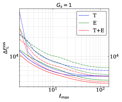
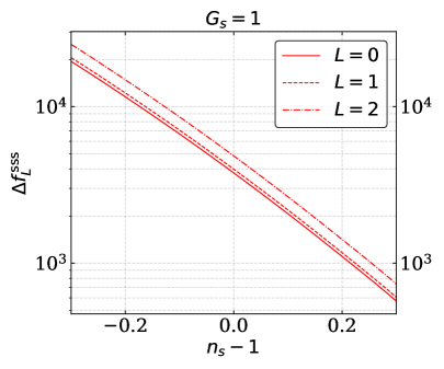
Figure 2: Plot of the expected 1-sigma error on $f^{\rm sss}_{L}$ from $\mu T$ and $\mu E$ for a PIXIE-like level of noise. Plain lines corresponds to $L=0$, dashed lines to $L=1$, dot-dashed lines to $L=2$. Left Panel: $\Delta f_{L}^{\rm sss}$ vs $\ell_{\rm max}$ for scale invariant scalar power spectrum. Right panel: $\Delta f_{L}^{\rm sss}$ vs $n_{s}-1$.

In fig. 2 we plot the expected 1-sigma error on $f_{L}^{sss}$ for different kind of statistical anisotropies labeled by $L=0,1,2$ obtained combining the $C^{\mu T}_{\ell m}$ and $C^{\mu E}_{\ell m}$ angular cross-spectra. The plots are made taking $G_{s}=1$ and varying the scalar-tilt at the SD scales. From our numerical results we obtain the following scaling formula

$$\Delta f_{L}^{sss}|_{T+E}=a\,10^{b(n_{s}-1)+c(n_{s}-1)^{2}}\,.$$ (4.21)

Analyzing the expression for the Fisher matrix (4.18), this formula can be generalized to $G_{s}\neq 1$ and with generic level of noise $\mu_{N}$ as

$$\Delta f_{L}^{sss}|_{T+E}=\frac{a}{G_{s}}\,\left(\frac{\mu_{\rm N}}{4.96\times 10^{-8}}\right)\,10^{b(n_{s}-1)+c(n_{s}-1)^{2}}\,.$$ (4.22)

In tab. 1 we summarize the values of the fit parameters $a$, $b$, $c$ for the various $L$-poles.

$L$	$a$	$b$	$c$
0	$3.7\times 10^{3}$	$-2.55$	$-0.58$
1	$3.9\times 10^{3}$	$-2.55$	$-0.58$
2	$4.8\times 10^{3}$	$-2.55$	$-0.58$

Table 1: Values of the parameters in eq. (4.22).

Our results suggest that the detectability prospects decrease by increasing the $L$-pole labelling a given statistical anisotropy. However, by admitting statistical anisotropies with $L\leq 2$, the detectability prospects remain commensurate.

4.2 2-tensors 1-scalar bispectrum

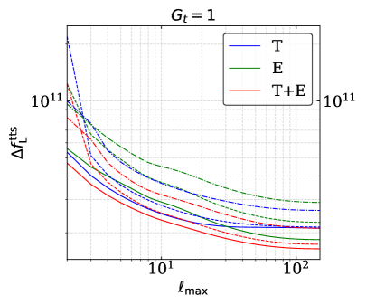
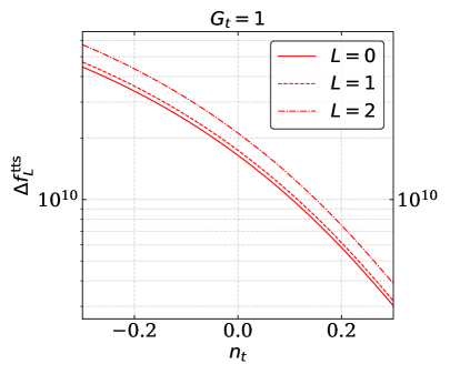
Figure 3: Plot of the expected 1-sigma error on $f^{\rm tts}_{L}$ from $\mu T$ and $\mu E$ for PIXIE-like noise. The tensor-to-scalar ratio at CMB scales is taken $r_{\rm CMB}=0.01$. Plain lines corresponds to $L=0$, dashed lines to $L=1$, dot-dashed lines to $L=2$. Left Panel: $\Delta f_{L}^{\rm tts}$ vs $\ell_{\rm max}$ for scale invariant tensor power spectrum. Right panel: $\Delta f_{L}^{\rm tts}$ vs $n_{t}$.

As in the previous subsection, SD-CMB cross-correlators sensitive to the 2-tensors 1-scalar primordial bispectrum are $C^{\mu T}_{\ell_{1}\ell_{2}m_{1}m_{2}}$ and $C^{\mu E}_{\ell_{1}\ell_{2}m_{1}m_{2}}$ angular cross-spectra. By substituting (3.2) and (3.3) into (4.4) we get

$$A_{\ell_{1}\ell_{2}}^{LM,\,\mu T}= \,\,\,i^{\ell_{1}-\ell_{2}}\,\sqrt{(2\ell_{1}+1)(2\ell_{2}+1)}\,\begin{pmatrix}\ell_{1}&\ell_{2}&L\\ 0&0&0\end{pmatrix}$$

$$\times\,8\pi\,\left(\sum_{\lambda\lambda^{\prime}}\xi_{\lambda\lambda^{\prime}}\right)\,\mathcal{I}^{\ell_{1}\ell_{2},LM,T}_{\gamma\gamma\zeta}\,,$$ (4.23)

and

$$A_{\ell_{1}\ell_{2}}^{LM,\,\mu E}= \,\,\,i^{\ell_{1}-\ell_{2}}\,\sqrt{(2\ell_{1}+1)(2\ell_{2}+1)}\,\begin{pmatrix}\ell_{1}&\ell_{2}&L\\ 0&0&0\end{pmatrix}$$

$$\times\,8\pi\,\left(\sum_{\lambda\lambda^{\prime}}\xi_{\lambda\lambda^{\prime}}\right)\,\mathcal{I}^{\ell_{1}\ell_{2},LM,E}_{\gamma\gamma\zeta}\,,$$ (4.24)

where $\mathcal{I}^{\ell_{1}\ell_{2},LM,T}_{\gamma\gamma\zeta}$ and $\mathcal{I}^{\ell_{1}\ell_{2},LM,E}_{\gamma\gamma\zeta}$ are as in eqs. (3.16) and (3.32). Here we adopt the convention $|\xi_{RR}|=|\xi_{LL}|=1$, and we assume $\xi_{LR}=\xi_{RL}=0$ . In fig. 3 we plot the expected 1-sigma error on $f^{tts}_{L}$ for $L=0,1,2$. Using the plots and the expression of the Fisher matrix we can get the following scaling formula of the expected 1-sigma error

$$\Delta f_{L}^{tts}|_{T+E}=\frac{a}{G_{t}}\,\left(\frac{\mu_{\rm N}}{4.96\times 10^{-8}}\right)\,\left(\frac{0.01}{r_{\rm CMB}}\right)10^{b(n_{t})+c(n_{t})^{2}}\,,$$ (4.25)

where $r_{\rm CMB}$ denotes the tensor-to-scalar ratio at CMB scales, and the values of the parameters are given in tab. 2.

$L$	$a$	$b$	$c$
0	$1.6\times 10^{10}$	$-1.91$	$-1.52$
1	$1.7\times 10^{10}$	$-1.91$	$-1.52$
2	$2.1\times 10^{10}$	$-1.91$	$-1.52$

Table 2: Values of the parameters in eq. (4.25).

Again, we notice a degradation in the detection prospects with increasing levels of statistical anisotropies, while the dependence on the other relevant parameters is not altered by the kind of statistical anisotropy.

4.3 2-scalars 1-tensor bispectrum

Intuitively, the SD-CMB cross-correlation most sensitive to the 2-scalars 1-tensor primordial bispectrum is the $C^{\mu B}_{\ell_{1}\ell_{2}m_{1}m_{2}}$ cross-spectrum. In fact, cross-correlations of $\mu$ modes with $T$ and $E$ modes generated by tensor perturbations are expected to be limited by the scalar induced cosmic variance-limited $T$- and $E$-mode power spectra. On large scales, the CMB tensor transfer functions ${\cal T}_{\ell(t)}^{X}$ are comparable in size to the scalar transfer functions ${\cal T}_{\ell(s)}^{X}$. Therefore, the $\mu T(\mu E)$ and $\mu B$ Fisher matrices per unit-$\ell$ scale as

$$\frac{F_{L}^{\mu T}}{F_{L}^{\mu B}}\Big{|}_{\ell}\sim\frac{C_{\ell}^{BB}}{C_{\ell}^{TT}}\sim r_{\rm CMB}\,.$$ (4.26)

As $r_{\rm CMB}<0.056$, we have an increase of at least 1 order of magnitude in the 1-sigma error on $f^{sst}_{L}$ by using $\mu T$ and $\mu E$ rather than $\mu B$.

By substituting eq. (3.4) into eq. (4.4) and employing the properties of the Wigner symbols we get

$$A_{\ell_{1}\ell_{2}}^{LM,\,\mu B}= \,\,i^{\ell_{1}-\ell_{2}}\,\sqrt{(2\ell_{1}+1)(2\ell_{2}+1)}\,\begin{pmatrix}\ell_{1}&\ell_{2}&L\\ 0&2&-2\end{pmatrix}$$

$$\times\,4\pi\,\mathcal{I}^{\ell_{1}\ell_{2},LM,B}_{\zeta\zeta\gamma}\,,$$ (4.27)

where $\mathcal{I}^{\ell_{1}\ell_{2},LM,B}_{\zeta\zeta\gamma}$ is as in eq. (3.4). Here we adopt the convention $|\xi_{R}|=|\xi_{L}|=1$.

The computation of the Fisher matrix for $f^{tss}_{L}$ resembles the computations above and we get

$$F_{L}=\sum_{\ell_{1},\ell_{2}=2}^{\ell_{\rm max}}\frac{\tilde{A}_{\ell_{1}\ell_{2}}^{LM,\,\mu B}\,\tilde{A}_{\ell_{1}\ell_{2}}^{*LM,\,\mu B}}{C^{\mu\mu}_{\ell_{1},\rm N}\,C^{BB}_{\ell_{2}}}\,,$$ (4.28)

where $\tilde{A}_{\ell_{1}\ell_{2}}^{LM,\,\mu B}=\partial A_{\ell_{1}\ell_{2}}^{LM,\,\mu B}/\partial f^{sst}_{L}$. In fig. 4 we plot the expected 1-sigma error on $f^{sst}_{L}$, with $L=2$, for the different ways in which the $\langle\zeta\zeta\gamma\rangle$ bispectrum transforms under parity transformation.

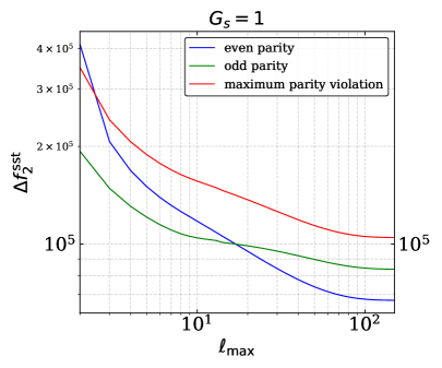
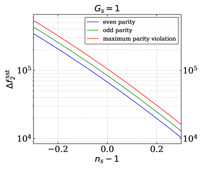
Figure 4: Plot of the expected 1-sigma error on $f^{\rm sst}_{2}$ from $\mu B$ for PIXIE-like level of noise and cosmic-variance limited fully delensed $B$ modes. The tensor-to-scalar ratio at CMB scales is taken $r_{\rm CMB}=0.01$. Left Panel: $\Delta f_{2}^{\rm sst}$ vs $\ell_{\rm max}$ for scale invariant scalar power spectrum. Right panel: $\Delta f_{2}^{\rm sst}$ vs $n_{s}-1$.

From the results of the forecasts and the expression of the Fisher matrix, we obtain the following scaling formula

$$\Delta f_{2}^{sst}|_{B}=\frac{a}{G_{s}}\,\left(\frac{\mu_{\rm N}}{4.96\times 10^{-8}}\right)\,\left(\frac{0.01}{r_{\rm CMB}}\right)^{1/2}\,10^{b(n_{s}-1)+c(n_{s}-1)^{2}}\,.$$ (4.29)

In tab. 3 we summarize the values of the fit parameters $a$, $b$, $c$.

Transformation under parity	$a$	$b$	$c$
even parity	$6.8\times 10^{4}$	$-2.55$	$-0.58$
odd parity	$8.5\times 10^{4}$	$-2.55$	$-0.58$
maximum parity violation	$1.0\times 10^{5}$	$-2.55$	$-0.58$

Table 3: Values of the parameters in eq. (4.29).

Here we have only explored the case of quadrupolar statistical anisotropies ($L=2$). Higher levels of statistical anisotropies can be studied as well, but we leave such a study for more model dependent settings. We found that detectability prospects slighly degrade when we consider parity violation signatures, even if the final results still remain commensurate.

4.4 3-tensors bispectrum

Analogously to the previous subsection, the SD-CMB cross-correlation most sensitive to the 3-tensors primordial bispectrum is the $C^{\mu B}_{\ell_{1}\ell_{2}m_{1}m_{2}}$ cross-spectrum. The Fisher matrix reads

$$F=\sum_{\ell_{1},\ell_{2}=2}^{\ell_{\rm max}}\frac{\tilde{A}_{\ell_{1}\ell_{2}}^{LM,\,\mu B}\,\tilde{A}_{\ell_{1}\ell_{2}}^{*LM,\,\mu B}}{C^{\mu\mu}_{\ell_{1},\rm N}\,C^{BB}_{\ell_{2}}}\,,$$ (4.30)

where $\tilde{A}_{\ell_{1}\ell_{2}}^{LM,\,\mu B}=\partial A_{\ell_{1}\ell_{2}}^{LM,\,\mu B}/\partial f^{ttt}_{L}$ and

$$A_{\ell_{1}\ell_{2}}^{LM,\,\mu B}= \,\,i^{\ell_{1}-\ell_{2}}\,\sqrt{(2\ell_{1}+1)(2\ell_{2}+1)}\,\begin{pmatrix}\ell_{1}&\ell_{2}&L\\ 0&2&-2\end{pmatrix}$$

$$\times\,8\pi\,\mathcal{I}^{\ell_{1}\ell_{2},LM,B}_{\gamma\gamma\gamma}\,,$$ (4.31)

where $\mathcal{I}^{\ell_{1}\ell_{2},LM,B}_{\gamma\gamma\gamma}$ is as in eq. (3.4). Here we adopt the convention $|\xi_{RRR}|=|\xi_{LLL}|=1$, and we assume $\xi_{RRL}=\xi_{LLR}=0$ . In fig. 5 we plot the expected 1-sigma error on $f^{ttt}_{L}$ with $L=2$ for the various ways in which the $\langle\gamma\gamma\gamma\rangle$ bispectrum transforms under parity transformation.

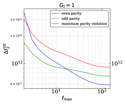
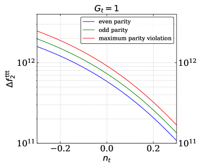
Figure 5: Plot of the expected 1-sigma error on $f^{\rm ttt}_{2}$ from $\mu B$ for a PIXIE-like level of noise and cosmic-variance limited fully delensed $B$ modes. The tensor-to-scalar ratio at CMB scales is taken $r_{\rm CMB}=0.01$. Left panel: $\Delta f_{2}^{\rm ttt}$ vs $\ell_{\rm max}$ for scale invariant tensor power spectrum. Right panel: $\Delta f_{2}^{\rm ttt}$ vs $n_{t}$.

From our plots and the Fisher matrix we obtain the following scaling formula

$$\Delta f_{2}^{ttt}|_{B}=\frac{a}{G_{t}}\,\left(\frac{\mu_{\rm N}}{4.96\times 10^{-8}}\right)\,\left(\frac{0.01}{r_{\rm CMB}}\right)^{1/2}\,10^{b(n_{t})+c(n_{t})^{2}}\,.$$ (4.32)

In tab. 4 we summarize the values of the fit parameters $a$, $b$, $c$.

Transformation under parity	$a$	$b$	$c$
even parity	$5.9\times 10^{11}$	$-1.91$	$-1.52$
odd parity	$7.3\times 10^{11}$	$-1.91$	$-1.52$
maximum parity violation	$9.0\times 10^{11}$	$-1.91$	$-1.52$

Table 4: Values of the parameters in eq. (4.32).

As before, we have a slight dependence on the level of parity violation, while the dependence on the other relevant parameters is not altered by the level of parity violation.

In the next section, we make some considerations about what we learn from these forecasts and their validity. We also discuss various classes of inflationary models that could be of relevance for the observables we are considering.

5 Model considerations

In this section, we consider various phenomenological and model building aspects of our findings. We begin by commenting on the assumption of weak NGs. In performing our Fisher matrix forecasts in the previous section, we implicitly assumed that primordial NGs are small compared to the Gaussian part of the primordial correlators. Demanding that non-linear effects from a given squeezed primordial correlation $\langle xx^{\prime}x^{\prime\prime}\rangle$ are subdominant than the linear results, translates into the following condition

$$k_{l}^{3}k_{s}^{3}\,\langle x(k_{l})x^{\prime}(k_{s})x^{\prime\prime}(k_{s})\rangle\ll\Delta_{x}(k_{l})\Delta_{x^{\prime}}(k_{s})\Delta_{x^{\prime\prime}}(k_{s})\,,$$ (5.1)

where $\Delta_{i}=(\mathcal{A}_{i})^{1/2}$ denote the square roots of the dimensionless power spectra. By applying eq. (5.1) to primordial bispectra we get the following constraints to our non-Gaussian amplitudes

$$f_{L}^{tts},\,f_{L}^{sss} \ll\Big{(}\mathcal{A}_{s}(k_{\rm CMB})\Big{)}^{-1}\simeq 10^{5}\,,$$ (5.2)

$$f_{L}^{sst},\,f_{L}^{ttt} \ll\Big{(}\mathcal{A}_{s}(k_{\rm CMB})\,r_{\rm CMB}\Big{)}^{-1}\simeq\frac{10^{5}}{r_{\rm CMB}}\,.$$ (5.3)

These theoretical upper bounds should be matched with the 1-sigma error derived from the plots above. Assuming almost scale invariant spectra in the window of scales where primordial perturbations source $\mu$-distortions, we got the following rough expressions for a PIXIE-like experiment

$$\Delta f_{L}^{tts}\approx\frac{10^{10}}{G_{T}}\left(\frac{0.01}{r_{\rm CMB}}\right)^{1/2}\,,\quad\Delta f_{L}^{sss}\approx\frac{10^{3}}{G_{s}}\,,\quad\Delta f_{L}^{sst}\approx\frac{10^{4}}{G_{s}}\left(\frac{0.01}{r_{\rm CMB}}\right)^{1/2}\,,\quad\Delta f_{L}^{ttt}\approx\frac{10^{11}}{G_{T}}\left(\frac{0.01}{r_{\rm CMB}}\right)^{1/2}\,.$$ (5.4)

Assuming $r_{\rm CMB}\sim 0.01-0.001$ and the absence of growth-mechanisms ($G_{i}=1$), we get that the expected 1-sigma error on $\langle\gamma\gamma\gamma\rangle$ and $\langle\gamma\gamma\zeta\rangle$ is larger than the theoretical upper bound. This is something that was expected if we look at fig. 1. The tensor $\mu$ modes transfer function is about five orders of magnitude smaller than the scalar transfer function. Therefore, in absence of mechanisms of amplifications of primordial perturbations we would expect

$$\Delta f_{L}^{tts}\approx 10^{-5}\,r_{\rm CMB}\,\Delta f_{L}^{sss}\,,\qquad\qquad\Delta f_{L}^{ttt}\approx 10^{-5}\,r_{\rm CMB}\,\Delta f_{L}^{sst}\,,$$ (5.5)

which is in agreement with (5.4) for $G_{i}=1$. From eq. (5.5) it follows that we need the following amplification of the tensor perturbations amplitude

$$G_{T}\approx\frac{10^{5}}{r_{\rm CMB}}$$ (5.6)

in order for $\langle\gamma\gamma\gamma\rangle$ and $\langle\gamma\gamma\zeta\rangle$ bispectra to reach the same level of detectability as $\langle\zeta\zeta\zeta\rangle$ and $\langle\zeta\zeta\gamma\rangle$. In absence of such an amplification of tensor perturbations, $\langle\gamma\gamma\gamma\rangle$ and $\langle\gamma\gamma\zeta\rangle$ bispectra are basically unconstrained by the cross-correlators between CMB $\mu$ modes and CMB temperature and polarization anisotropies. Given the current upper bound on $r_{\rm CMB}$ from the Planck experiment, we need an amplification factor of at least $G_{T}\gtrsim 10^{6}$, (and proportionally more if $G_{s}$ is also greater than one). Such a huge, independent amplification of tensor inflationary perturbations in the $\mu$ modes-era is typically not reachable within a controlled approximation in inflationary models known to us. As noticed e.g. in [96], only gravitational waves of post-inflationary origin appear to be realistic targets for $\mu$-distortions experiments. This suggests that from our current vantage point $\langle\zeta\zeta\zeta\rangle$ and $\langle\zeta\zeta\gamma\rangle$ are most likely the only bispectra we may put realistic constraints using the cross-correlations we are considering. However, model builders may some day concoct a model that successfully independently amplifies primordial tensor perturbations with $G_{T}\gtrsim 10^{6}$.

By including the sky-damping factor $f_{\rm sky}$, we also get the scaling formulas

$$\Delta f_{L}^{sss}|_{T+E}\sim\frac{10^{3}}{G_{s}\,f_{\rm sky}}\left(\frac{\mu_{\rm N}}{4.96\times 10^{-8}}\right)\,10^{-2.55(n_{s}-1)-0.58(n_{s}-1)^{2}}\,,$$

$$\Delta f_{L}^{sst}|_{B}\sim\frac{10^{4}}{G_{s}\,f_{\rm sky}}\left(\frac{\mu_{\rm N}}{4.96\times 10^{-8}}\right)\left(\frac{0.01}{r_{\rm CMB}}\right)^{1/2}\,10^{-2.55(n_{s}-1)-0.58(n_{s}-1)^{2}}\,.$$ (5.7)

Combining these equations we get the following scaling

$$\Delta f_{L}^{sst}|_{B}\sim 10\left(\frac{0.01}{r_{\rm CMB}}\right)^{1/2}\Delta f_{L}^{sss}|_{T+E}\,.$$ (5.8)

Assuming $r_{\rm CMB}=0.01$ we get that $\mathcal{O}(1)$ squeezed non-Gaussian $\langle\zeta\zeta\zeta\rangle$ ($\langle\zeta\zeta\gamma\rangle$) amplitudes can be measured if the amplification of scalar perturbations satisfies $G_{s}>10^{3}\,(10^{4})$. These results are particularly interesting since models with such amplification in the power spectra typically also share an analogous amplification of the non-Gaussian amplitudes.

Examples of such scenarios are inflationary models of primordial black hole (PBH) production (see, e.g., [101, 102, 103, 104, 105, 106, 107, 108]). As shown e.g. in [109], though an ultra-slow-roll mechanism we can enhance the power spectrum of scalar perturbations up to seven orders of magnitude, reaching $G_{s}=10^{7}$. Assuming such an amplification mechanism and an experiment with a PIXIE-like level of noise with $f_{\rm sky}=0.1$ and $r_{\rm CMB}=0.01$, this would lead to $\Delta f_{L}^{sss}\simeq 10^{-3}$ and $\Delta f_{L}^{sst}\simeq 10^{-2}$. However, it is worth to stress that the presence of even a low level of statistical anisotropies in these bispectra is necessary to get non-trivial signatures. To our knowledge, the effects of statistical anisotropies in such models is still unexplored.

Similarly, interesting detection prospects have already been considered in literature for the pure scalar (isotropic) bispectrum $\langle\zeta\zeta\zeta\rangle$ from the $\mu T$ and $\mu E$ cross-correlations (see e.g. [38, 43, 109]). Here we want to emphasize that in those models in which statistical anisotropies in the $\langle\zeta\zeta\zeta\rangle$ bispectrum leave detectable signatures in $\mu T$ and $\mu E$, there is also a possibility to detect a non-zero $\langle\zeta\zeta\gamma\rangle$ bispectrum signal from the $\mu B$ cross-correlator. This is relevant as the $\langle\zeta\zeta\gamma\rangle$ bispectrum reveals information on the underlying inflationary scenario that are usually not contained in the $\langle\zeta\zeta\zeta\rangle$ bispectrum. For example, a measurement or constraint on $\langle\zeta\zeta\gamma\rangle$ would allow us to probe: (i) the interactions between scalar and tensor primordial perturbations, (ii) the gravitational waves induced by second order scalar perturbations, (iii) a deeper insight in the violation of rotational and parity symmetries in the primordial universe. In particular, this last feature is rather interesting. As we have shown in sec. 3.5, depending on the kind of statistical anisotropy and the way in which the $\langle\zeta\zeta\gamma\rangle$ bispectrum transforms under parity symmetry we are able to predict the multipole configurations that provide a non-zero signal. This implies that a detection of a non-zero $\langle\mu_{\ell_{1}}B_{\ell_{2}}\rangle$ signal in certain $\ell_{1},\ell_{2}$ doublets may provide detailed information about the violation of the parity symmetry in inflationary models. Needless to say, a similar argument applies also to $\langle\mu_{\ell_{1}}T_{\ell_{2}}\rangle$ and $\langle\mu_{\ell_{1}}E_{\ell_{2}}\rangle$ cross-correlations. In this case, parity violation signatures may be left imprinted also by the $\langle\zeta\zeta\zeta\rangle$ bispectrum with $L_{1}=\mbox{odd}$, $L_{2}=0$ statistical anisotropies. However, when $L_{1}=\mbox{even}$, we must rely solely on $\langle\gamma\zeta\zeta\rangle$ to probe parity violation.

In order for tensor NGs to be meaningfully detectable via SD-CMB cross correlations, one evidently requires a large amplification of scalar and/or tensor modes at scales relevant for $\mu$-distortions, which moreover, must be sourced by a background that also violates statistical isotropy. Although this may seem like a doubly contrived demand, there is evidently a class of models for which the violation of statistical isotropy and the amplification of primordial perturbations may go hand in hand. Inflation realized via a scalar field charged under a U(1) symmetry with an inflaton dependent gauge kinetic coupling has been studied by the authors of [110, 111] as a means to generate observable levels of statistical anisotropy. The model action is given by

$$S=\int d^{4}x\sqrt{-g}\left[\frac{M_{P}^{2}}{2}R-\frac{1}{2}D_{\mu}\phi D^{\mu}\bar{\phi}-\frac{f^{2}(\phi)}{4}F_{\mu\nu}F^{\mu\nu}-V(\phi,\bar{\phi})\right].$$ (5.9)

A non-zero expectation value for the gauge potential (which breaks isotropy) is sustained during inflation through a combination of the gauge kinetic mixing and the minimal coupling of the charged scalar to the U(1) field. The inflaton potential can correspond to a range of universality classes, including hilltop, hybrid, and chaotic inflation, implying a large degree of parametric freedom in this class of models [110, 111]. The presence of higher dimensional terms (in the power counting sense) implicit in the operator $f^{2}(\phi)F^{2}$ forces us to consider the above as an effective action, for which the additional interaction $g^{2}(\phi)F\widetilde{F}$ appears with the same degree of (ir)relevance. The presence of the latter term, which for the modulus of the charged scalar mimics that of an axionic coupling to $F\widetilde{F}$ has been shown to generically source large, secondarily produced primordial perturbations (e.g. [18, 16]). Although such an iteration of the class of models represented by Eq. (5.9) has not been studied in the literature to our knowledge, it is of equal relevance from a power counting perspective, and places the violation of statistical isotropy and the generation of enhanced scalars and tensors on an equal footing. The parametric freedom in the choices of the three independent functions $f(\phi),g(\phi)$ and $V(\phi)$ ought to be suggestive to any interested model builders as a possibility to generate the level of SD-CMB cross correlations relevant to the considerations of this paper.

We conclude this section by discussing some limitations of our forecasts. First, we stress that the $\Delta f^{xxx}_{L}$’s derived above represent only the lower bound on the 1-sigma error, and they corresponds to the exact error only when our observables are Gaussian distributed. In our case the BipoSH coefficients $A_{\ell_{1}\ell_{2}}^{LM,\mathcal{O}^{1}\mathcal{O}^{2}}$ approach a Gaussian distribution only in the large-$\ell_{1},\ell_{2}$ limit (see e.g. [112]). Since we are looking to relatively large scale effects (low CMB multipoles), it is most likely that the real 1-sigma error is higher than what stated. Also, we did not account for the contribution of galactic foregrounds. As noticed in [113, 114], these should be taken into account for a real world experiment. On the other end, our forecasts are valid assuming that the non-Gaussian amplitudes $f^{xxx}_{L}$ are almost scale invariant functions of the parameters of an underlying inflationary model. As shown in eq. (2.19), the squeezed limit amplitudes $f^{xxx}_{L}$ may depend on the short and soft modes $k_{s}$ and $k_{l}$. A scale dependence over $k_{s}$ and $k_{l}$ stronger than a logarithmic or a soft power law may modify our forecasts in a non-trivial way. In such a case one should reabsorb the scale dependence in a parameter $\alpha$ as

$$f^{xxx}_{L}(k_{s},k_{l})=\alpha(k_{s},k_{l})\,\tilde{f}^{xxx}_{L}\,,$$ (5.10)

where $\tilde{f}^{xxx}_{L}$ is a scale-invariant quantity. Therefore, we can reabsorb the quantity $\alpha(k_{s},k_{l})$ inside the momenta integrations of e.g. eq. (3.11). The final forecast should be made on $\tilde{f}^{xxx}_{L}$. Finally, we like to discuss the degradation of the detectability of $\langle\zeta\zeta\gamma\rangle$ due to lensing contamination on CMB $B$ modes. By reproducing the plot in fig. 4 accounting for the contribution of the lensed $B$ modes in the cosmic variance limit we get the results summarized in fig. 6 . As shown, for values of the tensor-to-scalar-ratio within the aim of the forthcoming CMB experiments ($r_{\rm CMB}=0.01,0.001$) the 1-sigma error increases at most a factor $2$, remaining of the same order of magnitude as the fully delensed case. This suggests that accounting for the lensing contamination in the cosmic variance limit will not significantly change the detectability prospects for the values of $r_{\rm CMB}$ that next generation of CMB experiments aims to measure.

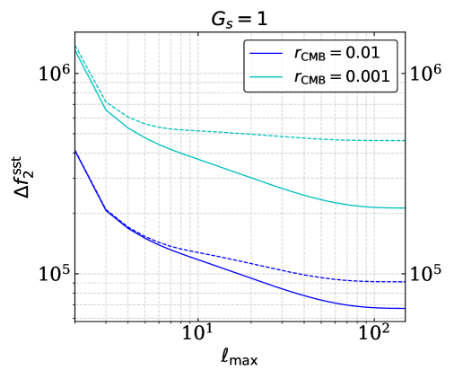
Figure 6: Plot of the expected 1-sigma error on $f^{\rm sst}_{2}$ for the parity even case as in fig. 4 obtained for different values of the tensor-to-scalar ratio at CMB scales. Straight lines: fully delensed $B$ modes. Dashed lines: lensed $B$ modes.

6 Conclusion

In this work we have explored new observational channels to probe tensor primordial NGs by exploiting the cross-correlations between the CMB $\mu$-distortions and temperature and polarization anisotropies. We have focused to the case where we introduce statistical anisotropies in squeezed NGs, as isotropic NGs leave either vanishing or highly suppressed signatures on the observables considered.

In detail, we have computed the effect of all the primordial (squeezed) bipectra involving both scalar and tensors on $\langle X_{\ell_{1}}\,\mu_{\ell_{2}}\rangle$ ($X=T,E,B$) cross-correlations. As statistical anisotropies in squeezed bispectra induce statistical anisotropies in these cross-correlations, we introduced the BipoSH formalism and BipoSH coefficients to study the detectability prospects through Fisher-matrix forecasts.

We found that $\langle\zeta\zeta\gamma\rangle$ and $\langle\zeta\zeta\zeta\rangle$ are the only bispectra where we could realistically observe statistical anisotropies by cross-correlating the observational channels of the current and forthcoming CMB experiments, like Planck, LiteBIRD, PICO and PIXIE-like or proble class missions. The signatures left by the $\langle\gamma\gamma\gamma\rangle$ and $\langle\gamma\gamma\zeta\rangle$ bispectra are limited by the corresponding $\langle\zeta\zeta\gamma\rangle$ and $\langle\zeta\zeta\zeta\rangle$ bispectra unless a mechanism generates huge, independent growth in tensor perturbations in the window of scales where primordial perturbations source $\mu$-distortions. In particular, tensor perturbations have to increase by over six orders of magnitude with respect to the current constraints placed by the Planck experiment. What makes the detection of $\langle\gamma\gamma\gamma\rangle$ and $\langle\gamma\gamma\zeta\rangle$ very challenging is that tensor perturbations dissipate their energy much more inefficiently than scalar perturbations.

We also found that for those inflationary models where the detection prospects of statistical anisotropies in the $\langle\zeta\zeta\zeta\rangle$ bispectrum are enhanced by combining the $\langle\mu_{\ell_{1}}T_{\ell_{2}}\rangle$ and $\langle\mu_{\ell_{1}}E_{\ell_{2}}\rangle$ information, also the detection prospects for probing statistical anisotropies in $\langle\zeta\zeta\gamma\rangle$ bispectrum from the cross-correlation $\langle\mu_{\ell_{1}}B_{\ell_{2}}\,\rangle$ are enhanced (see the model independent eq. (5.8)). This is relevant as it provides us with an observational channel complementary to the usual $\langle BB\rangle$ channel to find evidence of primordial gravitational waves in non-conventional models of inflation.

Our final eq. (5) aims to predict the level of detectability of the $\langle\zeta\zeta\zeta\rangle$ and $\langle\zeta\zeta\gamma\rangle$ non-Gaussian amplitudes defined in (2.19) and (2.20). Our forecasts are valid provided that in the window of scales where $\mu$ modes are produced we can approximate the scale dependence of the primordial power spectra as power-laws with almost constant spectral indexes, and assuming that the non-Gaussian amplitudes are almost constant. In case of more general scale-dependencies, a more detailed model-dependent analysis should be performed, using and adapting the results derived in sec. 3. However, the general claim that the detectability prospects of statistical anisotropies in $\langle\zeta\zeta\gamma\rangle$ bispectrum are enhanced wherever we realize a model able to enhance the detection prospects of statistical anisotropies in $\langle\zeta\zeta\zeta\rangle$ bispectrum, is universally valid, independently of the specific realization of inflation.

As a final remark, we stress that a detection of a net signature on the cross-correlations we have considered in this work would imply a realization of inflation containing very peculiar features, like huge growth mechanisms of primordial perturbations in a very localized window of scales, and the presence of a controlled level of statistical anisotropies which must be consistent with the bounds already placed by the current CMB experiments. These are stringent constraints on inflationary model building, where any candidate model has to simultaneously realize these two conditions. Henceforth, a detection of a signature through these channels with forthcoming CMB experiments would most likely be sourced by non-standard inflationary dynamics, possibly within the class of models represented in Eq. (5.9) with an additional interaction of the form $g^{2}(\phi)F\widetilde{F}$, although such a model has yet to be studied in the literature to our knowledge. We argue that the observational channels of primordial tensor NGs we proposed in this work will become important in a very futuristic scenario, where we will be able to exploit the cosmic variance limit level of noise in CMB experiments. In this regards, an analysis of the detection prospects of the signatures considered here in an ultimate survey is left for future research.

Acknowledgements

We want to thank Giovanni Cabass, Jens Chluba, Ema Dimastrogiovanni, Enrico Pajer, Andrea Ravenni, Maresuke Shiraishi, and Gianmassimo Tasinato for useful comments on the draft. We are grateful to Enrico Pajer for constructive criticism on our preliminary results. G.O. and P.D.M acknowledge support from the Netherlands organization for scientific research (NWO) VIDI grant (dossier 639.042.730).

Appendix A Spin-raising and lowering operators and spin-weighted spherical harmonics

Here, we briefly review the definitions of the spin-raising and lowering operators, giving an example on how we can use them to define the weighted spherical harmonics. We refer to e.g. [81] for more details. The spin raising $\;\raise 1.0pt\hbox{${}^{\prime}$}\hskip-6.0pt\partial\;$ and lowering $\;\overline{\raise 1.0pt\hbox{${}^{\prime}$}\hskip-6.0pt\partial}\;$ operators acting on a generic spin s function ${}_{s}f(\theta,\phi)$ defined on a 2D sphere are given by

$$\;\raise 1.0pt\hbox{${}^{\prime}$}\hskip-6.0pt\partial\;{}_{s}f(\theta,\phi) =-\sin^{s}\theta\left[\partial_{\theta}+i\csc\theta\partial_{\phi}\right]\sin^{-s}\theta{}_{s}f(\theta,\phi)~{},$$

$$\;\overline{\raise 1.0pt\hbox{${}^{\prime}$}\hskip-6.0pt\partial}\;{}_{s}f(\theta,\phi) =-\sin^{-s}\theta\left[\partial_{\theta}-i\csc\theta\partial_{\phi}\right]\sin^{s}\theta{}_{s}f(\theta,\phi)~{}.$$ (A.1)

In particular, the new functions $\;\raise 1.0pt\hbox{${}^{\prime}$}\hskip-6.0pt\partial\;{}_{s}f(\theta,\phi)$ and $\;\overline{\raise 1.0pt\hbox{${}^{\prime}$}\hskip-6.0pt\partial}\;{}_{s}f(\theta,\phi)$ have spin $s+1$ and $s-1$, respectively. For example, the spin raising and lowering operators acting twice on a generic spin-$\pm 2$ function ${}_{\pm 2}f(\mu,\phi)$ which is factorized as ${}_{\pm 2}f(\theta,\phi)={}_{\pm 2}\tilde{f}(\mu)e^{im\phi}$ (i.e. the CMB polarization fields) can be expressed as

$$\;\overline{\raise 1.0pt\hbox{${}^{\prime}$}\hskip-6.0pt\partial}\;^{2}{}_{2}f(\theta,\phi) =\left(-\partial_{\mu}+\frac{m}{1-\mu^{2}}\right)^{2}\left[(1-\mu^{2}){}_{2}f(\mu,\phi)\right]~{},$$

$$\;\raise 1.0pt\hbox{${}^{\prime}$}\hskip-6.0pt\partial\;^{2}{}_{-2}f(\theta,\phi) =\left(-\partial_{\mu}-\frac{m}{1-\mu^{2}}\right)^{2}\left[(1-\mu^{2}){}_{-2}f(\mu,\phi)\right]~{},$$ (A.2)

where $\mu\equiv\cos\theta$. In this way, just acting with a differential operator, we can easily define spin-0 quantities starting from spin-2 ones. This procedure is used in the case of CMB to pass from the $P^{\pm}$ spin-$\pm 2$ linear polarization fields to the $E$ and $B$ modes, which are spin-0 fields.

Using eqs. (A.1), we can express the spin-weighted spherical harmonic functions on a 2D sphere, ${}_{s}Y_{\ell m}(\theta,\phi)$, in terms of the common spherical harmonics ${}_{0}Y_{\ell m}(\theta,\phi)=Y_{\ell m}(\theta,\phi)$ by acting with the spin raising/lowering operator as

$${}_{s}Y_{\ell m}(\theta,\phi) =\left[\frac{(\ell-s)!}{(\ell+s)!}\right]^{\frac{1}{2}}\;\raise 1.0pt\hbox{${}^{\prime}$}\hskip-6.0pt\partial\;^{s}Y_{\ell m}(\theta,\phi)\ \ (0\leq s\leq\ell)~{},$$

$${}_{s}Y_{\ell m}(\theta,\phi) =\left[\frac{(\ell+s)!}{(\ell-s)!}\right]^{\frac{1}{2}}(-1)^{s}\;\overline{\raise 1.0pt\hbox{${}^{\prime}$}\hskip-6.0pt\partial}\;^{-s}Y_{\ell m}(\theta,\phi)\ \ (-\ell\leq s\leq 0)~{}.$$ (A.3)

Then, it is possible to show the validity of the following relations

$$\;\raise 1.0pt\hbox{${}^{\prime}$}\hskip-6.0pt\partial\;{}_{s}Y_{\ell m}(\theta,\phi) =\left[(\ell-s)(\ell+s+1)\right]^{\frac{1}{2}}\,{}_{s+1}Y_{\ell m}(\theta,\phi)~{},$$

$$\;\overline{\raise 1.0pt\hbox{${}^{\prime}$}\hskip-6.0pt\partial}\;{}_{s}Y_{\ell m}(\theta,\phi) =-\left[(\ell+s)(\ell-s+1)\right]^{\frac{1}{2}}\,{}_{s-1}Y_{\ell m}(\theta,\phi)~{},$$

$$\;\overline{\raise 1.0pt\hbox{${}^{\prime}$}\hskip-6.0pt\partial}\;\;\raise 1.0pt\hbox{${}^{\prime}$}\hskip-6.0pt\partial\;{}_{s}Y_{\ell m}(\theta,\phi) =-(\ell-s)(\ell+s+1)\,{}_{s}Y_{\ell m}(\theta,\phi)~{}m\,,$$ (A.4)

which can be used to derive the following explicit expression of the weighted spherical harmonics

$${}_{s}Y_{\ell m}(\theta,\phi) = e^{im\phi}\left[\frac{(\ell+m)!(\ell-m)!}{(\ell+s)!(\ell-s)!}\frac{(2\ell+1)}{4\pi}\right]^{1/2}\sin^{2\ell}(\theta/2)$$ (A.5)

$$\times\sum_{r}{\ell-s\choose r}{\ell+s\choose r+s-m}(-1)^{\ell-r-s+m}{\rm cot}^{2r+s-m}(\theta/2)~{}.$$

It is straightforward to verify the orthogonality and completeness conditions for the ${}_{s}Y_{\ell m}(\theta,\phi)$ as

$$\int_{0}^{2\pi}d\phi\int_{-1}^{1}d\cos\theta\,\,{}_{s}Y_{\ell^{\prime}m^{\prime}}^{*}(\theta,\phi)\,{}_{s}Y_{\ell m}(\theta,\phi) =\delta_{\ell^{\prime},\ell}\,\delta_{m^{\prime},m}~{},$$

$$\sum_{\ell m}{}_{s}Y_{\ell m}^{*}(\theta,\phi)\,{}_{s}Y_{\ell m}(\theta^{\prime},\phi^{\prime}) =\delta(\phi-\phi^{\prime})\delta(\cos\theta-\cos\theta^{\prime})\,,$$ (A.6)

as well as the following properties regarding the transformation under conjugate and parity

$${}_{s}Y^{*}_{\ell m}(\theta,\phi) =(-1)^{s+m}{}_{-s}Y_{\ell-m}(\theta,\phi)~{},$$

$${}_{s}Y_{\ell m}(\pi-\theta,\phi+\pi) =(-1)^{\ell}\,{}_{-s}Y_{\ell m}(\theta,\phi)~{}.$$ (A.7)

Appendix B 3-j symbols, Gaunt integral and Clebsch-Gordan coefficients

In this appendix, we give some useful formulas regarding the angular integrals of products of spherical harmonics. We will use $\hat{x}$ to denote a given direction on the 2D sphere and $d^{2}\Omega_{x}$ to indicate the infinitesimal solid angle on the sphere.

First, we define the quantity ${}_{s_{1}s_{2}s_{3}}\mathcal{G}_{\ell_{1}\ell_{2}\ell_{3}}^{m_{1}m_{2}m_{3}}$, which is known as "generalized" Gaunt integral and it represents the angular integral of the product of three (weighted) spherical harmonics. This can be written in terms of Wigner 3-j symbols as (see e.g. [115, 116])

$${}_{s_{1}s_{2}s_{3}}\mathcal{G}_{\ell_{1}\ell_{2}\ell_{3}}^{m_{1}m_{2}m_{3}} =\int d^{2}\Omega_{x}\,{}_{s_{1}}Y_{\ell_{1}m_{1}}(\hat{x})\,{}_{s_{2}}Y_{\ell_{2}m_{2}}(\hat{x})\,{}_{s_{3}}Y_{\ell_{3}m_{3}}(\hat{x})$$

$$=\sqrt{\frac{(2\ell_{1}+1)(2\ell_{2}+1)(2\ell_{3}+1)}{4\pi}}\begin{pmatrix}\ell_{1}&\ell_{2}&\ell_{3}\\ -s_{1}&-s_{2}&-s_{3}\end{pmatrix}\begin{pmatrix}\ell_{1}&\ell_{2}&\ell_{3}\\ m_{1}&m_{2}&m_{3}\end{pmatrix}\,.$$ (B.1)

The Wigner 3-j symbols are related to the spin-weighted spherical harmonics as

$$\prod_{i=1}^{2}{}_{s_{i}}Y_{\ell_{i}m_{i}}(\hat{x}) =\sum_{\ell_{3}m_{3}s_{3}}\,{}_{s_{3}}Y^{*}_{\ell_{3}m_{3}}(\hat{x})\,\sqrt{\frac{(2\ell_{1}+1)(2\ell_{2}+1)(2\ell_{3}+1)}{4\pi}}$$

$$\times\begin{pmatrix}\ell_{1}&\ell_{2}&\ell_{3}\\ -s_{1}&-s_{2}&-s_{3}\end{pmatrix}\begin{pmatrix}\ell_{1}&\ell_{2}&\ell_{3}\\ m_{1}&m_{2}&m_{3}\end{pmatrix}\,.$$ (B.2)

Notice that eq. (B) follows once putting together eqs. (A) and (B).

Some useful properties of the Wigner 3-j symbols that we used in this work are

$$\begin{pmatrix}\ell_{1}&\ell_{2}&\ell_{3}\\ m_{1}&m_{2}&m_{3}\end{pmatrix}=(-1)^{\sum_{i}\ell_{i}}\begin{pmatrix}\ell_{1}&\ell_{2}&\ell_{3}\\ -m_{1}&-m_{2}&-m_{3}\end{pmatrix}\,,$$ (B.3)

and

$$\sum_{m_{1},m_{2}}\begin{pmatrix}\ell_{1}&\ell_{2}&\ell_{3}\\ m_{1}&m_{2}&m_{3}\end{pmatrix}\begin{pmatrix}\ell_{1}&\ell_{2}&\ell^{\prime}_{3}\\ m_{1}&m_{2}&m^{\prime}_{3}\end{pmatrix}=(2\ell_{3}+1)^{-1}\,\delta_{\ell_{3},\ell^{\prime}_{3}}\,\delta_{m_{3},m^{\prime}_{3}}\,.$$ (B.4)

The 3-j symbols of the kind

$$\begin{pmatrix}\ell_{1}&\ell_{2}&\ell_{3}\\ m_{1}&m_{2}&-m_{3}\end{pmatrix}$$ (B.5)

are related to the Clebsh-Gordan coefficients

$$\mathcal{C}^{\ell_{2}m_{3}}_{\ell_{1}m_{1}\ell_{2}m_{2}}=\langle\ell_{1}m_{1}\ell_{2}m_{2}|\ell_{3}m_{3}\rangle$$ (B.6)

by [117]

$$\begin{pmatrix}\ell_{1}&\ell_{2}&\ell_{3}\\ m_{1}&m_{2}&-m_{3}\end{pmatrix}=\frac{(-1)^{\ell_{1}-\ell_{2}+m_{3}}}{\sqrt{2\ell_{3}+1}}\,\mathcal{C}^{\ell_{2}m_{3}}_{\ell_{1}m_{1}\ell_{2}m_{2}}\,.$$ (B.7)

Therefore, the 3-j symbols of the form (B.5) vanish unless the selection rules are satisfied as follows

$$|m_{1}|\leq\ell_{1}\,,\qquad|m_{2}|\leq\ell_{2}\,,\qquad|m_{3}|\leq\ell_{3}\,,\qquad m_{1}+m_{2}=m_{3}\,,$$ (B.8)

$$|\ell_{1}-\ell_{2}|\leq\ell_{3}\leq\ell_{1}+\ell_{2}\quad\mbox{(the triangle condition)}\,,\qquad\ell_{1}+\ell_{2}+\ell_{3}\in Z\,.$$ (B.9)

More properties of the Wigner 3-j symbols can be found in [117].

References

- [1] J. M. Maldacena, Non-Gaussian features of primordial fluctuations in single field inflationary models, JHEP 05 (2003) 013, [astro-ph/0210603].
- [2] X. Chen, Primordial Non-Gaussianities from Inflation Models, Adv. Astron. 2010 (2010) 638979, [1002.1416].
- [3] Planck collaboration, Y. Akrami et al., Planck 2018 results. IX. Constraints on primordial non-Gaussianity, 1905.05697.
- [4] M. Shiraishi, Tensor Non-Gaussianity Search: Current Status and Future Prospects, Front. Astron. Space Sci. 6 (2019) 49, [1905.12485].
- [5] V. De Luca, G. Franciolini, A. Kehagias, A. Riotto and M. Shiraishi, Constraining graviton non-Gaussianity through the CMB bispectra, Phys. Rev. D 100 (2019) 063535, [1908.00366].
- [6] M. Mylova, O. Özsoy, S. Parameswaran, G. Tasinato and I. Zavala, A new mechanism to enhance primordial tensor fluctuations in single field inflation, JCAP 12 (2018) 024, [1808.10475].
- [7] C. T. Byrnes, P. S. Cole and S. P. Patil, Steepest growth of the power spectrum and primordial black holes, JCAP 06 (2019) 028, [1811.11158].
- [8] P. Carrilho, K. A. Malik and D. J. Mulryne, Dissecting the growth of the power spectrum for primordial black holes, Phys. Rev. D 100 (2019) 103529, [1907.05237].
- [9] O. Özsoy and G. Tasinato, On the slope of the curvature power spectrum in non-attractor inflation, JCAP 04 (2020) 048, [1912.01061].
- [10] O. Ozsoy, M. Mylova, S. Parameswaran, C. Powell, G. Tasinato and I. Zavala, Squeezed tensor non-Gaussianity in non-attractor inflation, JCAP 09 (2019) 036, [1902.04976].
- [11] G. Tasinato, An analytic approach to non-slow-roll inflation, Phys. Rev. D 103 (2021) 023535, [2012.02518].
- [12] D. Wands, Multiple field inflation, Lect. Notes Phys. 738 (2008) 275–304, [astro-ph/0702187].
- [13] C. T. Byrnes and K.-Y. Choi, Review of local non-Gaussianity from multi-field inflation, Adv. Astron. 2010 (2010) 724525, [1002.3110].
- [14] L. Bordin, P. Creminelli, A. Khmelnitsky and L. Senatore, Light Particles with Spin in Inflation, JCAP 10 (2018) 013, [1806.10587].
- [15] E. Dimastrogiovanni, M. Fasiello, G. Tasinato and D. Wands, Tensor non-Gaussianities from Non-minimal Coupling to the Inflaton, JCAP 02 (2019) 008, [1810.08866].
- [16] N. Barnaby and M. Peloso, Large Nongaussianity in Axion Inflation, Phys. Rev. Lett. 106 (2011) 181301, [1011.1500].
- [17] A. Maleknejad and M. Sheikh-Jabbari, Gauge-flation: Inflation From Non-Abelian Gauge Fields, Phys. Lett. B 723 (2013) 224–228, [1102.1513].
- [18] J. L. Cook and L. Sorbo, An inflationary model with small scalar and large tensor nongaussianities, JCAP 11 (2013) 047, [1307.7077].
- [19] T. Fujita, J. Yokoyama and S. Yokoyama, Can a spectator scalar field enhance inflationary tensor mode?, PTEP 2015 (2015) 043E01, [1411.3658].
- [20] E. Dimastrogiovanni, M. Fasiello and T. Fujita, Primordial Gravitational Waves from Axion-Gauge Fields Dynamics, JCAP 01 (2017) 019, [1608.04216].
- [21] Y. Watanabe and E. Komatsu, Gravitational Wave from Axion-SU(2) Gauge Fields: Effective Field Theory for Kinetically Driven Inflation, 2004.04350.
- [22] R. Holman and A. J. Tolley, Enhanced Non-Gaussianity from Excited Initial States, JCAP 05 (2008) 001, [0710.1302].
- [23] N. Agarwal, R. Holman, A. J. Tolley and J. Lin, Effective field theory and non-Gaussianity from general inflationary states, JHEP 05 (2013) 085, [1212.1172].
- [24] S. Akama, S. Hirano and T. Kobayashi, Primordial tensor non-Gaussianities from general single-field inflation with non-Bunch-Davies initial states, Phys. Rev. D 102 (2020) 023513, [2003.10686].
- [25] S. Endlich, A. Nicolis and J. Wang, Solid Inflation, JCAP 1310 (2013) 011, [1210.0569].
- [26] S. Endlich, B. Horn, A. Nicolis and J. Wang, Squeezed limit of the solid inflation three-point function, Phys. Rev. D90 (2014) 063506, [1307.8114].
- [27] N. Bartolo, D. Cannone, A. Ricciardone and G. Tasinato, Distinctive signatures of space-time diffeomorphism breaking in EFT of inflation, JCAP 03 (2016) 044, [1511.07414].
- [28] N. Bartolo and G. Orlando, Parity breaking signatures from a Chern-Simons coupling during inflation: the case of non-Gaussian gravitational waves, JCAP 1707 (2017) 034, [1706.04627].
- [29] N. Bartolo, G. Orlando and M. Shiraishi, Measuring chiral gravitational waves in Chern-Simons gravity with CMB bispectra, JCAP 01 (2019) 050, [1809.11170].
- [30] A. Ricciardone and G. Tasinato, Primordial gravitational waves in supersolid inflation, Phys. Rev. D 96 (2017) 023508, [1611.04516].
- [31] A. Ricciardone and G. Tasinato, Anisotropic tensor power spectrum at interferometer scales induced by tensor squeezed non-Gaussianity, JCAP 02 (2018) 011, [1711.02635].
- [32] L. Mirzagholi, E. Komatsu, K. D. Lozanov and Y. Watanabe, Effects of Gravitational Chern-Simons during Axion-SU(2) Inflation, JCAP 06 (2020) 024, [2003.05931].
- [33] M. Celoria, D. Comelli, L. Pilo and R. Rollo, Boosting GWs in Supersolid Inflation, JHEP 01 (2021) 185, [2010.02023].
- [34] N. Bartolo, L. Caloni, G. Orlando and A. Ricciardone, Tensor non-Gaussianity in chiral scalar-tensor theories of gravity, JCAP 03 (2021) 073, [2008.01715].
- [35] L. Bordin and G. Cabass, Graviton non-Gaussianities and Parity Violation in the EFT of Inflation, 2004.00619.
- [36] G. Cabass, Zoology of Graviton non-Gaussianities, 2103.09816.
- [37] M. Celoria, D. Comelli, L. Pilo and R. Rollo, Primordial Non-Gaussianity in Supersolid Inflation, 2103.10402.
- [38] E. Pajer and M. Zaldarriaga, A New Window on Primordial non-Gaussianity, Phys. Rev. Lett. 109 (2012) 021302, [1201.5375].
- [39] R. Emami, E. Dimastrogiovanni, J. Chluba and M. Kamionkowski, Probing the scale dependence of non-Gaussianity with spectral distortions of the cosmic microwave background, Phys. Rev. D 91 (2015) 123531, [1504.00675].
- [40] M. Shiraishi, M. Liguori, N. Bartolo and S. Matarrese, Measuring primordial anisotropic correlators with CMB spectral distortions, Phys. Rev. D 92 (2015) 083502, [1506.06670].
- [41] R. Khatri and R. Sunyaev, Constraints on -distortion fluctuations and primordial non-Gaussianity from Planck data, JCAP 09 (2015) 026, [1507.05615].
- [42] A. Ota, Cosmological constraints from cross-correlations, Phys. Rev. D 94 (2016) 103520, [1607.00212].
- [43] A. Ravenni, M. Liguori, N. Bartolo and M. Shiraishi, Primordial non-Gaussianity with -type and y-type spectral distortions: exploiting Cosmic Microwave Background polarization and dealing with secondary sources, JCAP 09 (2017) 042, [1707.04759].
- [44] G. Cabass, E. Pajer and D. van der Woude, Spectral distortion anisotropies from single-field inflation, JCAP 08 (2018) 050, [1805.08775].
- [45] M. Remazeilles, A. Ravenni and J. Chluba, Leverage on small-scale primordial non-Gaussianity through cross-correlations between CMB -mode and -distortion anisotropies, 2110.14664.
- [46] L. Iacconi, M. Fasiello, H. Assadullahi and D. Wands, Small-scale Tests of Inflation, 2008.00452.
- [47] P. Adshead, N. Afshordi, E. Dimastrogiovanni, M. Fasiello, E. A. Lim and G. Tasinato, Multimessenger cosmology: Correlating cosmic microwave background and stochastic gravitational wave background measurements, Phys. Rev. D 103 (2021) 023532, [2004.06619].
- [48] A. Malhotra, E. Dimastrogiovanni, M. Fasiello and M. Shiraishi, Cross-correlations as a Diagnostic Tool for Primordial Gravitational Waves, JCAP 03 (2021) 088, [2012.03498].
- [49] E. Dimastrogiovanni, M. Fasiello, A. Malhotra, P. D. Meerburg and G. Orlando, Testing the Early Universe with Anisotropies of the Gravitational Wave Background, 2109.03077.
- [50] N. Dalal, O. Doré, D. Huterer and A. Shirokov, The imprints of primordial non-gaussianities on large-scale structure: scale dependent bias and abundance of virialized objects, Phys. Rev. D77 (2008) 123514, [0710.4560].
- [51] S. Matarrese and L. Verde, The effect of primordial non-Gaussianity on halo bias, Astrophys. J. 677 (2008) L77–L80, [0801.4826].
- [52] D. Jeong and M. Kamionkowski, Clustering Fossils from the Early Universe, Phys. Rev. Lett. 108 (2012) 251301, [1203.0302].
- [53] E. Dimastrogiovanni, M. Fasiello, D. Jeong and M. Kamionkowski, Inflationary tensor fossils in large-scale structure, JCAP 12 (2014) 050, [1407.8204].
- [54] J. B. Muñoz, Y. Ali-Haïmoud and M. Kamionkowski, Primordial non-gaussianity from the bispectrum of 21-cm fluctuations in the dark ages, Phys. Rev. D 92 (2015) 083508, [1506.04152].
- [55] A. Hajian and T. Souradeep, Measuring statistical isotropy of the CMB anisotropy, Astrophys. J. Lett. 597 (2003) L5–L8, [astro-ph/0308001].
- [56] T. Souradeep and A. Hajian, Statistical isotropy of the Cosmic Microwave Background, Pramana 62 (2004) 793–796, [astro-ph/0308002].
- [57] A. Hajian and T. Souradeep, The Cosmic microwave background bipolar power spectrum: Basic formalism and applications, astro-ph/0501001.
- [58] A. Suzuki et al., The LiteBIRD Satellite Mission - Sub-Kelvin Instrument, J. Low Temp. Phys. 193 (2018) 1048–1056, [1801.06987].
- [59] M. Hazumi et al., LiteBIRD: A Satellite for the Studies of B-Mode Polarization and Inflation from Cosmic Background Radiation Detection, J. Low Temp. Phys. 194 (2019) 443–452.
- [60] NASA PICO collaboration, S. Hanany et al., PICO: Probe of Inflation and Cosmic Origins, 1902.10541.
- [61] A. Kogut et al., The Primordial Inflation Explorer (PIXIE): A Nulling Polarimeter for Cosmic Microwave Background Observations, JCAP 1107 (2011) 025, [1105.2044].
- [62] A. Kogut, M. Abitbol, J. Chluba, J. Delabrouille, D. Fixsen, J. Hill et al., CMB Spectral Distortions: Status and Prospects, 1907.13195.
- [63] J. Delabrouille et al., Microwave Spectro-Polarimetry of Matter and Radiation across Space and Time, 1909.01591.
- [64] S. Alexander and J. Martin, Birefringent gravitational waves and the consistency check of inflation, Phys. Rev. D 71 (2005) 063526, [hep-th/0410230].
- [65] T. Tanaka and Y. Urakawa, Dominance of gauge artifact in the consistency relation for the primordial bispectrum, JCAP 1105 (2011) 014, [1103.1251].
- [66] P. Creminelli, A. Perko, L. Senatore, M. Simonović and G. Trevisan, The Physical Squeezed Limit: Consistency Relations at Order , JCAP 1311 (2013) 015, [1307.0503].
- [67] E. Pajer, F. Schmidt and M. Zaldarriaga, The Observed Squeezed Limit of Cosmological Three-Point Functions, Phys. Rev. D88 (2013) 083502, [1305.0824].
- [68] V. Sreenath, D. K. Hazra and L. Sriramkumar, On the scalar consistency relation away from slow roll, JCAP 02 (2015) 029, [1410.0252].
- [69] V. Sreenath and L. Sriramkumar, Examining the consistency relations describing the three-point functions involving tensors, JCAP 10 (2014) 021, [1406.1609].
- [70] L. Bordin, P. Creminelli, M. Mirbabayi and J. Noreña, Solid Consistency, JCAP 03 (2017) 004, [1701.04382].
- [71] R. Bravo, S. Mooij, G. A. Palma and B. Pradenas, A generalized non-Gaussian consistency relation for single field inflation, JCAP 05 (2018) 024, [1711.02680].
- [72] B. Finelli, G. Goon, E. Pajer and L. Santoni, Soft Theorems For Shift-Symmetric Cosmologies, Phys. Rev. D 97 (2018) 063531, [1711.03737].
- [73] Y.-F. Cai, X. Chen, M. H. Namjoo, M. Sasaki, D.-G. Wang and Z. Wang, Revisiting non-Gaussianity from non-attractor inflation models, JCAP 05 (2018) 012, [1712.09998].
- [74] S. Jazayeri, E. Pajer and D. van der Woude, Solid Soft Theorems, JCAP 06 (2019) 011, [1902.09020].
- [75] R. Bravo and G. A. Palma, Unifying attractor and non-attractor models of inflation under a single soft theorem, 2009.03369.
- [76] T. Suyama, Y. Tada and M. Yamaguchi, Revisiting non-Gaussianity in non-attractor inflation models in the light of the cosmological soft theorem, PTEP 2021 (2021) 073E02, [2101.10682].
- [77] M. Shiraishi, Parity violation in the CMB trispectrum from the scalar sector, Phys. Rev. D 94 (2016) 083503, [1608.00368].
- [78] Planck collaboration, Y. Akrami et al., Planck 2018 results. X. Constraints on inflation, 1807.06211.
- [79] A. Kosowsky, Cosmic microwave background polarization, Annals Phys. 246 (1996) 49–85, [astro-ph/9501045].
- [80] W. Hu and M. J. White, CMB anisotropies: Total angular momentum method, Phys. Rev. D 56 (1997) 596–615, [astro-ph/9702170].
- [81] M. Zaldarriaga and U. Seljak, An all sky analysis of polarization in the microwave background, Phys. Rev. D 55 (1997) 1830–1840, [astro-ph/9609170].
- [82] S. Dodelson, Modern Cosmology. Academic Press, Amsterdam, 2003.
- [83] M. Shiraishi, S. Yokoyama, K. Ichiki and K. Takahashi, Analytic formulae of the CMB bispectra generated from non-Gaussianity in the tensor and vector perturbations, Phys. Rev. D 82 (2010) 103505, [1003.2096].
- [84] M. Shiraishi, D. Nitta, S. Yokoyama, K. Ichiki and K. Takahashi, CMB Bispectrum from Primordial Scalar, Vector and Tensor non-Gaussianities, Prog. Theor. Phys. 125 (2011) 795–813, [1012.1079].
- [85] A. Lewis, “CAMB Notes.”.
- [86] Planck collaboration, N. Aghanim et al., Planck 2018 results. VI. Cosmological parameters, 1807.06209.
- [87] R. Sunyaev and Y. Zeldovich, Small scale fluctuations of relic radiation, Astrophys. Space Sci. 7 (1970) 3–19.
- [88] R. Daly, Spectral distortions of the microwave background radiation resulting from the damping of pressure waves, The Astrophysical Journal 371 (1991) 14–28.
- [89] J. D. Barrow and P. Coles, Primordial density fluctuations and the microwave background spectrum, Monthly Notices of the Royal Astronomical Society 248 (01, 1991) 52–57, [https://academic.oup.com/mnras/article-pdf/248/1/52/18195181/mnras248-0052.pdf].
- [90] W. Hu, D. Scott and J. Silk, Power spectrum constraints from spectral distortions in the cosmic microwave background, Astrophys. J. Lett. 430 (1994) L5–L8, [astro-ph/9402045].
- [91] J. Chluba et al., Spectral Distortions of the CMB as a Probe of Inflation, Recombination, Structure Formation and Particle Physics: Astro2020 Science White Paper, Bull. Am. Astron. Soc. 51 (2019) 184, [1903.04218].
- [92] J. Chluba and R. A. Sunyaev, The evolution of CMB spectral distortions in the early Universe, Mon. Not. Roy. Astron. Soc. 419 (2012) 1294–1314, [1109.6552].
- [93] J. Chluba, A. L. Erickcek and I. Ben-Dayan, Probing the inflaton: Small-scale power spectrum constraints from measurements of the CMB energy spectrum, Astrophys. J. 758 (2012) 76, [1203.2681].
- [94] A. Ota, T. Takahashi, H. Tashiro and M. Yamaguchi, CMB distortion from primordial gravitational waves, JCAP 1410 (2014) 029, [1406.0451].
- [95] J. Chluba, L. Dai, D. Grin, M. Amin and M. Kamionkowski, Spectral distortions from the dissipation of tensor perturbations, Mon. Not. Roy. Astron. Soc. 446 (2015) 2871–2886, [1407.3653].
- [96] T. Kite, A. Ravenni, S. P. Patil and J. Chluba, Bridging the gap: spectral distortions meet gravitational waves, 2010.00040.
- [97] J. Chluba, E. Dimastrogiovanni, M. A. Amin and M. Kamionkowski, Evolution of CMB spectral distortion anisotropies and tests of primordial non-Gaussianity, Mon. Not. Roy. Astron. Soc. 466 (2017) 2390–2401, [1610.08711].
- [98] J. Ganc and E. Komatsu, Scale-dependent bias of galaxies and mu-type distortion of the cosmic microwave background spectrum from single-field inflation with a modified initial state, Phys. Rev. D86 (2012) 023518, [1204.4241].
- [99] E. Dimastrogiovanni and R. Emami, Correlating CMB Spectral Distortions with Temperature: what do we learn on Inflation?, JCAP 12 (2016) 015, [1606.04286].
- [100] A. Kalaja, P. D. Meerburg, G. L. Pimentel and W. R. Coulton, Fundamental limits on constraining primordial non-Gaussianity, JCAP 04 (2021) 050, [2011.09461].
- [101] J. Garcia-Bellido and E. Ruiz Morales, Primordial black holes from single field models of inflation, Phys. Dark Univ. 18 (2017) 47–54, [1702.03901].
- [102] J. M. Ezquiaga, J. Garcia-Bellido and E. Ruiz Morales, Primordial Black Hole production in Critical Higgs Inflation, Phys. Lett. B 776 (2018) 345–349, [1705.04861].
- [103] G. Ballesteros and M. Taoso, Primordial black hole dark matter from single field inflation, Phys. Rev. D 97 (2018) 023501, [1709.05565].
- [104] M. P. Hertzberg and M. Yamada, Primordial Black Holes from Polynomial Potentials in Single Field Inflation, Phys. Rev. D 97 (2018) 083509, [1712.09750].
- [105] M. Cicoli, V. A. Diaz and F. G. Pedro, Primordial Black Holes from String Inflation, JCAP 06 (2018) 034, [1803.02837].
- [106] O. Özsoy, S. Parameswaran, G. Tasinato and I. Zavala, Mechanisms for Primordial Black Hole Production in String Theory, JCAP 07 (2018) 005, [1803.07626].
- [107] R. Mahbub, Primordial black hole formation in inflationary -attractor models, Phys. Rev. D 101 (2020) 023533, [1910.10602].
- [108] G. Ballesteros, J. Rey, M. Taoso and A. Urbano, Primordial black holes as dark matter and gravitational waves from single-field polynomial inflation, JCAP 07 (2020) 025, [2001.08220].
- [109] O. Özsoy and G. Tasinato, CMB cross-correlations as a probe of PBH scenarios, 2104.12792.
- [110] R. Emami, H. Firouzjahi and M. S. Movahed, Inflation from Charged Scalar and Primordial Magnetic Fields?, Phys. Rev. D 81 (2010) 083526, [0908.4161].
- [111] R. Emami, Anisotropic Inflation and Cosmological Observations. PhD thesis, Hong Kong U. Sci. Tech., 2015. 1511.01683.
- [112] N. Joshi, A. Rotti and T. Souradeep, Statistics of Bipolar Representation of CMB maps, Phys. Rev. D 85 (2012) 043004, [1109.0729].
- [113] M. H. Abitbol, J. Chluba, J. C. Hill and B. R. Johnson, Prospects for Measuring Cosmic Microwave Background Spectral Distortions in the Presence of Foregrounds, Mon. Not. Roy. Astron. Soc. 471 (2017) 1126–1140, [1705.01534].
- [114] M. Remazeilles and J. Chluba, Extracting foreground-obscured -distortion anisotropies to constrain primordial non-Gaussianity, Mon. Not. Roy. Astron. Soc. 478 (2018) 807–824, [1802.10101].
- [115] E. Komatsu, D. N. Spergel and B. D. Wandelt, Measuring primordial non-Gaussianity in the cosmic microwave background, Astrophys. J. 634 (2005) 14–19, [astro-ph/0305189].
- [116] M. Liguori, F. Hansen, E. Komatsu, S. Matarrese and A. Riotto, Testing primordial non-gaussianity in cmb anisotropies, Phys. Rev. D 73 (2006) 043505, [astro-ph/0509098].
- [117] M. Shiraishi, Probing the Early Universe with the CMB Scalar, Vector and Tensor Bispectrum. Springer Theses. Springer, 2013. 10.1007/978-4-431-54180-6.