Heisenberg homology on surface configurations

Abstract

Motivated by the Lawrence-Krammer-Bigelow representations of the classical braid groups, we study the homology of unordered configurations in an orientable genus-$g$ surface with one boundary component, over non-commutative local systems defined from representations of the discrete Heisenberg group. For a general representation of the Heisenberg group we obtain a twisted representation of the mapping class group. For the linearisation of the affine translation action of the Heisenberg group we obtain a genuine, untwisted representation of the mapping class group. In the case of the Schrödinger representation or its finite-dimensional analogues, by composing with a Stone-von Neumann isomorphism we obtain a representation to the projective unitary group, which lifts to a unitary representation of the stably universal central extension of the mapping class group.

2020 MSC: 57K20, 55R80, 55N25, 20C12, 19C09
Key words: Mapping class groups, configuration spaces, homological representations, discrete Heisenberg group, Schrödinger representation, Morita’s crossed homomorphism.

Introduction

The braid group $B_{m}$ was defined by Artin in terms of geometric braids in $\mathbb{R}^{3}$; equivalently, it is the fundamental group of the configuration space $\mathcal{C}_{m}(\mathbb{R}^{2})$ of $m$ unordered points in the plane. Another equivalent description is as the mapping class group $\mathfrak{M}(\mathbb{D}_{m})=\mathrm{Diff}(\mathbb{D}_{m},S^{1})/\mathrm{Diff}_{0}(\mathbb{D}_{m},S^{1})$ of the closed $2$-disc with $m$ interior points removed. (The mapping class group of a surface is the group of isotopy classes of self-diffeomorphisms fixing the boundary pointwise.)

There is also a natural action of $\mathrm{Diff}(\mathbb{D}_{m},S^{1})$ on configuration spaces $\mathcal{C}_{n}(\mathbb{D}_{m})$; considering the induced action on the homology of these configuration spaces, Lawrence [28] defined a representation of $B_{m}$ for each $n\geqslant 1$. The $n=2$ version is known as the Lawrence-Krammer-Bigelow representation, and a celebrated result of Bigelow [12] and Krammer [27] states that this representation of $B_{m}$ is faithful, i.e. injective.

On the other hand, for almost all other surfaces $\Sigma$, the question of whether the mapping class group $\mathfrak{M}(\Sigma)$ admits a faithful, finite-dimensional representation over a field (whether it is linear) is open. The mapping class group of the torus is $SL_{2}(\mathbb{Z})$, which is evidently linear, and the mapping class group of the closed orientable surface of genus $2$ was shown to be linear by Bigelow and Budney [13], as a corollary of the linearity of $B_{5}$. However, nothing is known in genus $g\geqslant 3$.

Our programme is to study the action of the positive-genus and connected-boundary mapping class groups $\mathfrak{M}(\Sigma_{g,1})$ on the homology of the configuration spaces $\mathcal{C}_{n}(\Sigma_{g,1})$, equipped with local systems that are similar to the Lawrence-Krammer-Bigelow construction. We first argue that abelian local systems would not be good enough. In general, for any surface $\Sigma$ and $n\geqslant 2$, the abelianisation of $\pi_{1}(\mathcal{C}_{n}(\Sigma))$ is canonically isomorphic to $H_{1}(\Sigma)\times C$, where $C$ is a cyclic group of order $\infty$ if $\Sigma$ is planar, of order $2n-2$ if $\Sigma=\mathbb{S}^{2}$ and of order $2$ in all other cases (see for example [16, Proposition 6.32]). In the case $\Sigma=\mathbb{D}_{m}$, the abelianisation is $\mathbb{Z}^{m}\times\mathbb{Z}$, and the Lawrence representations are defined using the local system given by the quotient $\pi_{1}(\mathcal{C}_{n}(\mathbb{D}_{m}))\twoheadrightarrow\mathbb{Z}^{m}\times\mathbb{Z}\twoheadrightarrow\mathbb{Z}\times\mathbb{Z}$, where the second map is addition of the first $m$ factors. However, in the non-planar case (in particular if $\Sigma=\Sigma_{g,1}$), we lose information by passing to the abelianisation, since the cyclic factor $C$ – which counts the self-winding or “writhe” of a loop of configurations – has order $2$ rather than order $\infty$.

To obtain a better analogue of the Lawrence representations in the setting $\Sigma=\Sigma_{g,1}$ for $g>0$, we consider instead a larger, non-abelian quotient of $\pi_{1}(\mathcal{C}_{n}(\Sigma))$, which is isomorphic to the discrete Heisenberg group $\mathcal{H}=\mathcal{H}(\Sigma)$, defined as the central extension of the first homology $H=H_{1}(\Sigma,\mathbb{Z})$ associated to the intersection $2$-cocycle. This is a $2$-nilpotent group that arises very naturally as a quotient of the surface braid group $\pi_{1}(\mathcal{C}_{n}(\Sigma))$ by forcing a single element to be central. In the case $n\geqslant 3$ it is known by [4] to be the $2$-nilpotentisation of the surface braid group (in fact it is the maximal nilpotent quotient of the surface braid group), but for $n=2$ it differs from the $2$-nilpotentisation. A key property of this Heisenberg quotient is that it still detects the self-winding (or “writhe”) of a loop of configurations without reducing modulo two. Any representation $V$ of the discrete Heisenberg group $\mathcal{H}(\Sigma)$ defines a local system on the configuration space $\mathcal{C}_{n}(\Sigma)$.

An and Ko studied in [1] extensions of the Lawrence-Krammer-Bigelow representations to homological representations of surface braid groups; see also [7]. Their purpose was to extend the homological representation of the classical braid group to some homology of configurations in an $n$-punctured surface and produce representations of the surface braid groups. In our case the surface has no punctures, and the goal is to represent the full mapping class group. Our constructions based on the Heisenberg quotient of the surface braid group have a similar flavour but are significantly simpler; moreover we obtain strong improvements by specialising to explicit representations.

We speculate about faithfulness results for our representations and linearity results for the mapping class group. This would involve two steps.

1. Prove that the action on the homology of the Heisenberg covering space of $\mathcal{C}_{n}(\Sigma)$ is faithful. Following Bigelow’s strategy, this would follow from a key lemma showing that an algebraic intersection form on homology detects the geometric intersection of curves on the surface.

2. Find a good finite-dimensional representation of the Heisenberg group that retains faithfulness.

It was shown in [14, 15] that the adjoint representation of quantum $sl(2)$ at roots of $1$ has a topological realisation as homology of configurations with local coefficients in the once-punctured torus. The local system used there is a special case of our construction which, although purely topological, has a strong quantum flavour. We believe that our contribution opens a programme for topological interpretations of quantum constructions and possible classical constructions of quantum invariants and TQFTs.

Notation 1.

Henceforth we will use the abbreviation $\Sigma=\Sigma_{g,1}$ for an integer $g\geqslant 1$.

General representations.

Our first main result is a calculation of a Borel-Moore relative homology group with coefficients twisted by any representation of the Heisenberg group, together with a twisted action of the mapping class group. In the following, $H_{*}^{BM}$ denotes Borel-Moore homology and $\mathcal{C}_{n}(\Sigma,\partial^{-}(\Sigma))$ is the properly embedded subspace of $\mathcal{C}_{n}(\Sigma)$ consisting of all configurations intersecting a given closed arc $\partial^{-}\Sigma\subset\partial\Sigma$. The twisted action is formulated as a representation of an action groupoid. The key point is that the mapping class group acts on the Heisenberg group which implies an action on our local systems. We denote by $f_{\mathcal{H}}\in\mathrm{Aut(\mathcal{H})}$ the automorphism induced by $f\in\mathfrak{M}(\Sigma)$. For a representation $\rho\colon\mathcal{H}\rightarrow GL(V)$ and $\tau\in\mathrm{Aut}(\mathcal{H})$, the $\tau$-twisted representation $\rho\circ\tau$ is denoted by ${}_{\tau}\!V$.

Theorem A (Theorems 10 and 21).

Let $n\geqslant 2$, $g\geqslant 1$ and let $V$ be a representation of the discrete Heisenberg group $\mathcal{H}=\mathcal{H}(\Sigma)$ over a ring $R$.
(a) The Borel-Moore homology module $H_{n}^{BM}(\mathcal{C}_{n}(\Sigma),\mathcal{C}_{n}(\Sigma,\partial^{-}(\Sigma));V)$ is isomorphic to the direct sum of $\left(\begin{array}[]{c}2g+n-1\\ n\\ \end{array}\right)$ copies of $V$. Furthermore, it is the only non-vanishing module in the graded module $H_{*}^{BM}(\mathcal{C}_{n}(\Sigma),\mathcal{C}_{n}(\Sigma,\partial^{-}(\Sigma));V)$.
(b) There is a natural twisted representation of the mapping class group $\mathfrak{M}(\Sigma)$ on the collection of $R$-modules

$$H_{n}^{BM}\bigl{(}\mathcal{C}_{n}(\Sigma),\mathcal{C}_{n}(\Sigma,\partial^{-}(\Sigma));{}_{\tau}\!V\bigr{)}\ ,\quad\tau\in\mathrm{Aut}(\mathcal{H})\ ,\$$

where the action of $f\in\mathfrak{M}(\Sigma)$ is

$$\mathcal{C}_{n}(f)_{*}\colon H_{n}^{BM}\bigl{(}\mathcal{C}_{n}(\Sigma),\mathcal{C}_{n}(\Sigma,\partial^{-}(\Sigma));{}_{\tau\circ f_{\mathcal{H}}}\!V\bigr{)}\longrightarrow H_{n}^{BM}\bigl{(}\mathcal{C}_{n}(\Sigma),\mathcal{C}_{n}(\Sigma,\partial^{-}(\Sigma));{}_{\tau}\!V\bigr{)}.$$ (1)

Remark 2.

The case of a trivial representation of $\mathcal{H}$ is already something interesting; indeed, connecting with Moriyama’s work [32], we will show that the Johnson filtration is recovered.

Remark 3.

The Heisenberg group $\mathcal{H}(\Sigma)$ can be realised as a group of $(g+2)\times(g+2)$ matrices; this gives a $(g+2)$-dimensional representation, which we refer to as its tautological representation. We then obtain, for each $n\geqslant 2$, a family of twisted representations with polynomially growing dimension equal to $(g+2)\left(\begin{array}[]{c}2g+n-1\\ n\\ \end{array}\right)$.

The linearised translation action.

The discrete Heisenberg group $\mathcal{H}$ has a natural affine structure over $\mathbb{Z}$ for which the left translation action $\mathcal{H}\curvearrowright\mathcal{H}$ is by affine automorphisms. The linearisation functor $\mathrm{Aff}_{\mathbb{Z}}\to\mathbb{Z}\text{-Mod}$ applied to this affine action gives a representation $L=\mathcal{H}\oplus\mathbb{Z}\cong\mathbb{Z}^{2g+2}$ of $\mathcal{H}$ over $\mathbb{Z}$. A key feature of this representation is that, for an automorphim $\tau$ of $\mathcal{H}$, the twisted representation ${}_{\tau}L$ is canonically isomorphic to $L$. We deduce a genuine (i.e. untwisted) representation of the mapping class group.

Theorem B (Theorem 25).

For each $n\geqslant 2$ and $g\geqslant 1$ there is a representation of the mapping class group ${\mathfrak{M}}(\Sigma)$ on the free $\mathbb{Z}$-module of rank $(2g+2)\left(\begin{array}[]{c}2g+n-1\\ n\\ \end{array}\right)$,

$$H_{n}^{BM}\bigl{(}\mathcal{C}_{n}(\Sigma),\mathcal{C}_{n}(\Sigma,\partial^{-}(\Sigma));L\bigr{)}.$$ (2)

The Schrödinger representation.

The famous Stone-von Neumann Theorem states that the Schrödinger representation $W\cong L^{2}(\mathbb{R}^{g})$ is, up to isomorphism, the unique unitary representation of the real Heisenberg group $\mathcal{H}_{\mathbb{R}}(\Sigma)$ with given non-trivial action of its centre determined by a non-zero real number $\hbar$ (the Planck constant). We also denote by $W$ this representation restricted to the discrete subgroup $\mathcal{H}=\mathcal{H}(\Sigma)\subset\mathcal{H}_{\mathbb{R}}(\Sigma)$. For $\tau\in\mathrm{Aut}(\mathcal{H})$ the twisted representation ${}_{\tau}W$ is isomorphic to $W$ as a unitary representation and the isomorphism is defined up to a unit complex number. Using such isomorphisms we may identify the twisted local system with the original one and obtain an untwisted representation of the mapping class group to the projective unitary group of the homology with local coefficients $W$. We build a linear lift of this projective action to the stably universal central extension $\widetilde{\mathfrak{M}}(\Sigma)$.

Theorem C (Theorem 37).

For each $n\geqslant 2$ and $g\geqslant 1$ there is a complex unitary representation of $\widetilde{\mathfrak{M}}(\Sigma)$ on the complex Hilbert space

$$\mathcal{V}_{n}=H_{n}^{BM}\bigl{(}\mathcal{C}_{n}(\Sigma),\mathcal{C}_{n}(\Sigma,\partial^{-}(\Sigma));W\bigr{)}$$ (3)

that lifts the natural projective action $\mathfrak{M}(\Sigma)\rightarrow PU(\mathcal{V}_{n})$.

The group $\widetilde{\mathfrak{M}}(\Sigma)$ on which we construct our linear representation is a central extension of the mapping class group $\mathfrak{M}(\Sigma)$ of the form:

$$1\to\mathbb{Z}\longrightarrow\widetilde{\mathfrak{M}}(\Sigma)\longrightarrow\mathfrak{M}(\Sigma)\to 1,$$ (4)

and is the stably universal central extension of $\mathfrak{M}(\Sigma)$, which we explain next.

The stably universal central extension.

A group $G$ has a universal central extension (an initial object in the category of central extensions of $G$) if and only if $H_{1}(G;\mathbb{Z})=0$ and it is of the form $0\to H_{2}(G;\mathbb{Z})\to\widetilde{G}\to G\to 1$ when it exists. For genus $g\geqslant 4$, we have $H_{1}(\mathfrak{M}(\Sigma_{g,1});\mathbb{Z})=0$ and $H_{2}(\mathfrak{M}(\Sigma_{g,1});\mathbb{Z})\cong\mathbb{Z}$. Moreover, there are natural inclusion maps

$$\mathfrak{M}(\Sigma_{1,1})\longrightarrow\mathfrak{M}(\Sigma_{2,1})\longrightarrow\cdots\longrightarrow\mathfrak{M}(\Sigma_{g,1})\longrightarrow\mathfrak{M}(\Sigma_{g+1,1})\longrightarrow\cdots,$$ (5)

which induce isomorphisms on $H_{1}(-;\mathbb{Z})$ and $H_{2}(-;\mathbb{Z})$ for $g\geqslant 4$ (by homological stability for mapping class groups of surfaces, due originally to Harer [23]; see [37, Theorem 1.1] for the optimal stability range). This implies that, for $g\geqslant 4$, the pullback along (5) of the universal central extension of $\mathfrak{M}(\Sigma_{g+1,1})$ to $\mathfrak{M}(\Sigma_{g,1})$ is the universal central extension of $\mathfrak{M}(\Sigma_{g,1})$. Hence we may define, for all $g\geqslant 1$, the stably universal central extension of $\mathfrak{M}(\Sigma_{g,1})$ to be the pullback along (5) of the universal central extension of $\mathfrak{M}(\Sigma_{h,1})$ for any $h\geqslant\mathrm{max}(g,4)$.

A finite-dimensional Schrödinger representation.

When the Planck constant is $2\pi$ times a rational number, the discrete Heisenberg group has finite-dimensional Schrödinger representations, which may be realised either by theta functions, by induction or by an abelian TQFT. We will follow [20, 21, 22], which connect nicely the different approaches when $\hbar=\frac{2\pi}{N}$ for a positive even integer $N$. We denote by $W_{N}=L^{2}((\mathbb{Z}/N)^{g})$ the $N^{g}$-dimensional representation that is the unique irreducible representation of the finite quotient $\mathcal{H}_{N}=\mathcal{H}/I_{N}$ of $\mathcal{H}$ by the normal subgroup $I_{N}=\{(2Nk,Nx)\mid k\in\mathbb{Z},x\in H\}$ where each central element $(k,0)$ acts by $e^{\frac{i\pi k}{N}}$. The analogue of the Stone-von Neumann Theorem in this context [21, Theorem 2.4] allows us to construct an untwisted representation of the mapping class group to a projective unitary group which also supports a linear lift to the stably universal central extension.

Theorem D (Theorem 38).

For each $g\geqslant 1$, $n\geqslant 2$ and $N\geqslant 2$ with $N$ even, there is a complex unitary representation of $\widetilde{\mathfrak{M}}(\Sigma)$ on the $\binom{2g+n-1}{n}N^{g}$-dimensional complex Hilbert space

$$\mathcal{V}_{N,n}=H_{n}^{BM}\bigl{(}\mathcal{C}_{n}(\Sigma),\mathcal{C}_{n}(\Sigma,\partial^{-}(\Sigma));W_{N}\bigr{)}$$ (6)

that lifts the natural projective action $\mathfrak{M}(\Sigma)\rightarrow PU(\mathcal{V}_{N,n})$.

Remark 4.

For any complex vector space $V$, the adjoint action of $GL(V)$ on $\mathrm{End}_{\mathbb{C}}(V)$ induces a canonical embedding $PGL(V)\hookrightarrow GL(\mathrm{End}_{\mathbb{C}}(V))$. Applying this to the natural projective action $\mathfrak{M}(\Sigma)\rightarrow PU(\mathcal{V}_{N,n})$, we obtain an untwisted complex representation

$$\mathfrak{M}(\Sigma)\longrightarrow GL(\mathrm{End}_{\mathbb{C}}(\mathcal{V}_{N,n}))$$ (7)

of dimension $\binom{2g+n-1}{n}^{2}N^{2g}$. We observe that:

Observation 5.

Injectivity of (7) is equivalent to the assertion that

$$\text{the pre-image of }\mathbb{C}^{*}\text{ along }\eqref{eq:athm:universal-central-fd}\colon\widetilde{\mathfrak{M}}(\Sigma)\to U(\mathcal{V}_{N,n})\text{ is equal to }\mathbb{Z},$$ (8)

where $\mathbb{C}^{*}$ means the scalar operators in $U(\mathcal{V}_{N,n})$ and $\mathbb{Z}$ refers to the kernel of (4). Thus a proof of (8) for any $(N,n)$ with $N,n\geqslant 2$ would imply that the mapping class group $\mathfrak{M}(\Sigma)$ is linear.

Kernels.

To describe an upper bound on the kernels of our representations, we first recall the Johnson filtration of the mapping class group.

The mapping class group $\mathfrak{M}(\Sigma)$ acts naturally on the fundamental group $\pi_{1}(\Sigma)$ of the surface. Each term of the lower central series of a group is fully invariant, so there is a well-defined induced action of $\mathfrak{M}(\Sigma)$ on the quotient $\pi_{1}(\Sigma)/\varGamma_{i+1}$, which is the largest $(i+1)$-step nilpotent quotient of $\pi_{1}(\Sigma)$. The Johnson filtration $\mathfrak{J}(*)$ is then defined by setting $\mathfrak{J}(i)$ to be the kernel of this induced action. Thus $\mathfrak{J}(0)$ is the whole mapping class group and $\mathfrak{J}(1)$ is the Torelli group. The intersection of all terms in the filtration is trivial, i.e., it is an exhaustive filtration of the mapping class group [26].

One may also consider the induced action of the mapping class group $\mathfrak{M}(\Sigma)$ on the universal metabelian quotient $\pi_{1}(\Sigma)/\pi_{1}(\Sigma)^{(2)}$ of the fundamental group of the surface (the quotient by its second derived subgroup); its kernel is the Magnus kernel of $\mathfrak{M}(\Sigma)$, which we denote by $\mathrm{Mag}(\Sigma)\subseteq\mathfrak{M}(\Sigma)$. In §6 (Proposition 41) we prove:

Proposition E (Proposition 41).

For each $n\geqslant 2$, $g\geqslant 1$, considering the regular representation $V=\mathbb{Z}[\mathcal{H}]$ of the discrete Heisenberg group $\mathcal{H}=\mathcal{H}(\Sigma)$, the kernel of the representation constructed in Theorem A is contained in $\mathfrak{J}(n)\cap\mathrm{Mag}(\Sigma)$.

Computability.

We emphasise that our representations are explicit and computable. First, the underlying $R$-module in Theorem A is a direct sum of finitely many copies of the $R$-module $V$ that underlies the chosen representation of the discrete Heisenberg group $\mathcal{H}(\Sigma)$. This is Theorem A(a); an explicit basis is described in Theorem 10.

Moreover, the actions of elements of the mapping class group on the canonical basis provided by Theorem 10 may be explicitly computed. To demonstrate this, we calculate in §7 explicit matrices for our representations in the case when $n=2$ and $V=\mathbb{Z}[\mathcal{H}]$ is the regular representation of $\mathcal{H}=\mathcal{H}(\Sigma)$. For example, when $g=1$, the Dehn twist around the boundary of $\Sigma_{1,1}$ acts by the $3\times 3$ matrix over $\mathbb{Z}[\mathcal{H}]=\mathbb{Z}[u^{\pm 1}]\langle a^{\pm 1},b^{\pm 1}\rangle/(ab=u^{2}ba)$ depicted in Figure 4 (page 4).

Outline.

In §1 we define and study the quotient $\mathcal{H}$ of the surface braid group. In §2 we study the Borel-Moore homology with local coefficients of configuration spaces on $\Sigma$, proving Theorem A(a) and showing in particular that, with coefficients in $V=\mathbb{Z}[\mathcal{H}]$, it is a free module with an explicit free generating set. Next, in §3, we show that the action of the mapping class group on the surface braid group descends to the Heisenberg quotient $\mathcal{H}$.

In §4 we construct twisted representations (Theorem A(b)) of the full mapping class group, as well as the untwisted representations associated to the linearised translation action $L=\mathcal{H}\oplus\mathbb{Z}$ (Theorem B). In §5 we prove Theorems C and D for the Schrödinger representation of $\mathcal{H}$ and its finite-dimensional analogues. In §6 we discuss connections with the Moriyama and Magnus representations of mapping class groups and deduce that the kernels of our twisted representations of $\mathfrak{M}(\Sigma)$ from Theorem A, with coefficients in $V=\mathbb{Z}[\mathcal{H}]$, are contained in the intersection of the Johnson filtration with the Magnus kernel.

In §7 we explain how to compute explicit matrices for our representations with respect to the free basis coming from §2. We carry out this computation in the case of configurations of $n=2$ points and where $V=\mathbb{Z}[\mathcal{H}]$ is the regular representation of $\mathcal{H}$; this special case of our construction is a direct analogue of the Lawrence-Krammer-Bigelow representations of the braid groups.

The first version of this paper also contained further results about untwisted representations of subgroups of the mapping class group on Heisenberg homology. In order to improve readability, we have moved this part to a separate article.

Acknowledgements.

This paper forms part of the PhD thesis of the third author. The first and third authors are thankful for the support of the Abdus Salam School of Mathematical Sciences. The second author is grateful to Arthur Soulié for several enlightening discussions about the Moriyama and Magnus representations and their kernels, and for pointing out the reference [35]. The second author was partially supported by a grant of the Romanian Ministry of Education and Research, CNCS - UEFISCDI, project number PN-III-P4-ID-PCE-2020-2798, within PNCDI III.

Contents

1. 1 A non-commutative local system on configuration spaces of surfaces
2. 2 Heisenberg homology
3. 3 Action of mapping classes
4. 4 Constructing the representations
5. 5 The Schrödinger local system
6. 6 Relation to the Moriyama and Magnus representations
7. 7 Computations for $n=2$
8. Appendix A: a deformation retraction through Lipschitz embeddings
9. Appendix B: signs in the intersection pairing formula
10. Appendix C: Sage computations

1 A non-commutative local system on configuration spaces of surfaces

Let $\Sigma=\Sigma_{g,1}$ be a compact, connected, orientable surface of genus $g\geqslant 1$ with one boundary component. For $n\geqslant 2$, the $n$-point unordered configuration space of $\Sigma$ is

$$\mathcal{C}_{n}(\Sigma)=\{\{c_{1},c_{2},...,c_{n}\}\subset\Sigma\mid c_{i}\neq c_{j}\text{ for }i\neq j\},$$

topologised as a quotient of a subspace of $\Sigma^{n}$. The surface braid group $\mathbb{B}_{n}(\Sigma)$ is then defined as $\mathbb{B}_{n}(\Sigma)=\pi_{1}(\mathcal{C}_{n}(\Sigma))$. We will use the presentation of this group given by Bellingeri and Godelle in [5], which in turn follows from Bellingeri’s presentation [3]. It has generators $\sigma_{1},\ldots,\sigma_{n-1}$, $\alpha_{1},\ldots,\alpha_{g}$, $\beta_{1},\ldots,\beta_{g}$ and relations:

$$\begin{cases}\,\text{({BR1}) }\,[\sigma_{i},\sigma_{j}]=1&\text{for }\lvert i-j\rvert\geqslant 2,\\ \,\text{({BR2}) }\,\sigma_{i}\sigma_{j}\sigma_{i}=\sigma_{j}\sigma_{i}\sigma_{j}&\text{for }\lvert i-j\rvert=1,\\ \,\text{({CR1}) }\,[\alpha_{r},\sigma_{i}]=[\beta_{r},\sigma_{i}]=1&\text{for }i>1\text{ and all }r,\\ \,\text{({CR2}) }\,[\alpha_{r},\sigma_{1}\alpha_{r}\sigma_{1}]=[\beta_{r},\sigma_{1}\beta_{r}\sigma_{1}]=1&\text{for all }r,\\ \,\text{({CR3}) }\,[\alpha_{r},\sigma^{-1}_{1}\alpha_{s}\sigma_{1}]=[\alpha_{r},\sigma^{-1}_{1}\beta_{s}\sigma_{1}]=&\\ \qquad\qquad\qquad=[\beta_{r},\sigma^{-1}_{1}\alpha_{s}\sigma_{1}]=[\beta_{r},\sigma^{-1}_{1}\beta_{s}\sigma_{1}]=1&\text{for all }r<s,\\ \,\text{({SCR}) }\,\sigma_{1}\beta_{r}\sigma_{1}\alpha_{r}\sigma_{1}=\alpha_{r}\sigma_{1}\beta_{r}&\text{for all }r.\end{cases}$$

We note that composition of loops is written from right to left. Our relation (CR3) is a slight modification of the relation (CR3) of [5], but it is equivalent to it via the relation (CR2).

The first homology group $H_{1}(\Sigma)=H_{1}(\Sigma;\mathbb{Z})$ is equipped with a symplectic intersection form

$$\omega\colon H_{1}(\Sigma)\times H_{1}(\Sigma)\longrightarrow\mathbb{Z}$$

and the Heisenberg group $\mathcal{H}=\mathcal{H}(\Sigma)$ is defined to be the central extension of $H_{1}(\Sigma)$ determined by the $2$-cocycle $\omega$. Concretely, it is the set-theoretic product $\mathbb{Z}\times H_{1}(\Sigma)$ with the operation

$$(k,x)(l,y)=(k+l+\omega(x,y),x+y).$$ (9)

Denote by $\psi\colon\mathcal{H}\twoheadrightarrow H_{1}(\Sigma)$ the projection onto the second factor and by $i\colon\mathbb{Z}\hookrightarrow\mathcal{H}$ the inclusion of the first factor; the central extension may then be written as:

There is a general recipe for computing a presentation of an extension of two groups, given presentations of these two groups and some information about the structure of the extension (we will use the formulation of [16, Appendix B]; an alternative reference is [25, §2.4.3]). In particular, for a central extension $1\to H\to G\to K\to 1$ with $H=\langle X|R\rangle$ and $K=\langle Y|S\rangle$, we have $G=\langle X\sqcup Y|R\sqcup\widetilde{S}\sqcup T\rangle$, where $\widetilde{S}$ is any collection of relations that are true in $G$ and that project to the relations $S$ in $K$ and where $T$ is a collection of relations saying that the generators $X$ are central in $G$.

Applying this to our setting, we obtain the following presentation of $\mathcal{H}$, where we write $u=(1,0)$ and where $a_{1},\ldots,a_{g}$, $b_{1},\ldots,b_{g}$ is a symplectic basis of $H_{1}(\Sigma)$.

Proposition 6.

The Heisenberg group $\mathcal{H}=\mathcal{H}(\Sigma)$ admits a presentation with generators $u$, $\tilde{a}_{i}=(0,a_{i})$, $\tilde{b}_{i}=(0,b_{i})$ for $1\leqslant i\leqslant g$ and relations:

$$\begin{cases}\,\text{all pairs of generators commute, except:}\\ \,\tilde{a}_{i}\tilde{b}_{i}=u^{2}\tilde{b}_{i}\tilde{a}_{i}\qquad\text{for each }i.\end{cases}$$ (10)

Proof. We apply the above procedure to the presentations $\mathbb{Z}=\langle X|R\rangle$ and $H_{1}(\Sigma)=\langle Y|S\rangle$ where $X=\{u\}$, $Y=\{\tilde{a}_{1},\ldots,\tilde{a}_{g},\tilde{b}_{1},\ldots,\tilde{b}_{g}\}$, the relations $R$ are empty and the relations $S$ say that all pairs of elements of $Y$ commute. The relations $T$ say that $u$ commutes with each of $\{\tilde{a}_{1},\ldots,\tilde{a}_{g},\tilde{b}_{1},\ldots,\tilde{b}_{g}\}$, so to show that (10) is a correct presentation of $\mathcal{H}$ it will suffice to show that the relations $\tilde{a}_{i}\tilde{b}_{i}=u^{2}\tilde{b}_{i}\tilde{a}_{i}$ and $\tilde{a}_{i}\tilde{b}_{j}=\tilde{b}_{j}\tilde{a}_{i}$ for $i\neq j$ are true in $\mathcal{H}$, because we may then take $\widetilde{S}$ to be this collection of relations, since it projects to $S$. To verify these, we compute that

$$\tilde{a}_{i}\tilde{b}_{j}=(0,a_{i}+b_{j})=(0,b_{j}+a_{i})=\tilde{b}_{i}\tilde{a}_{j}$$

since $\omega(a_{i},b_{j})=0$ when $i\neq j$, and

$$\tilde{a}_{i}\tilde{b}_{i}=(1,a_{i}+b_{i})=(1,b_{i}+a_{i})=(2,0)(-1,b_{i}+a_{i})=u^{2}\tilde{b}_{i}\tilde{a}_{i},$$

since $\omega(a_{i},b_{i})=1$ and $\omega(b_{i},a_{i})=-1$.   

It follows immediately from this presentation that:

Corollary 7.

For each $g\geqslant 1$ and $n\geqslant 2$, there is a natural surjective homomorphism

$$\phi\colon\mathbb{B}_{n}(\Sigma)\relbar\joinrel\twoheadrightarrow\mathcal{H}(\Sigma)$$

sending each $\sigma_{i}$ to $u$ and sending $\alpha_{i}\mapsto\tilde{a}_{i}$, $\beta_{i}\mapsto\tilde{b}_{i}$.

In the case $n\geqslant 3$, this quotient of the surface braid group has previously been considered in [4, 6, 7], which also consider the more general setting where $\Sigma$ is closed or has several boundary components. The alternative approach in these articles allows one to identify the kernel of $\phi$ as a characteristic subgroup. We include below a description of the kernel valid for all $n\geqslant 2$.

Proposition 8.

(a) For $n\geqslant 2$, the kernel of $\phi$ is the normal subgroup generated by the commutators $[\sigma_{1},x]$ for $x\in\mathbb{B}_{n}(\Sigma)$.
(b) For $n\geqslant 3$, the kernel of $\phi$ is the subgroup of $3$-commutators $\Gamma_{3}(\mathbb{B}_{n}(\Sigma))$.

For a proof of statement (b), we refer to [4, Theorem 2]. More precisely, statement (10) on page 1416 of [4] is the analogous fact for the closed surface $\Sigma_{g}$: that there is a surjective homomorphism $\mathbb{B}_{n}(\Sigma_{g})\twoheadrightarrow\mathcal{H}_{g}/\langle u^{2(n+g-1)}\rangle$ whose kernel is exactly $\Gamma_{3}(\mathbb{B}_{n}(\Sigma_{g}))$. The proof given there works also in our case where the surface has one boundary component and we do not quotient by $\langle u^{2(n+g-1)}\rangle$. In this paper we will use statement (a) and focus on the case $n=2$ in our explicit computations.

Proof. Let $K_{n}\subseteq\mathbb{B}_{n}(\Sigma)$ be the normal subgroup generated by the commutators $[\sigma_{1},x]$ for $x\in\mathbb{B}_{n}(\Sigma)$. The image $\phi(\sigma_{1})$ being central, we have $K_{n}\subseteq\ker(\phi)$, hence we see that $\phi$ may be factored through a surjective homomorphism $\overline{\phi}\colon\mathbb{B}_{n}(\Sigma)/K_{n}\rightarrow\mathcal{H}$. If we add centrality of $\sigma_{1}$ to the defining relations for $\mathbb{B}_{n}(\Sigma)$, we may:

• replace (BR2) by $\sigma_{i}=\sigma_{1}$ for all $i$,

• remove (BR1), (CR1) and (CR2),

• replace (CR3) by commutators of all pairs of generators except for $(\alpha_{r},\beta_{r})$,

• replace (SCR) with $\alpha_{r}\beta_{r}=\sigma_{1}^{2}\beta_{r}\alpha_{r}$.

Finally the presentations of $\mathbb{B}_{n}(\Sigma)/K_{n}$ and $\mathcal{H}$ coincide and $\overline{\phi}$ is an isomorphism, which proves (a).   

In contrast to the case of $n\geqslant 3$, the kernel $\mathrm{ker}(\phi)$ when $n=2$ lies strictly between the terms $\Gamma_{2}$ and $\Gamma_{3}$ of the lower central series of $\mathbb{B}_{2}(\Sigma)$.

Proposition 9.

There are proper inclusions

$$\Gamma_{3}(\mathbb{B}_{2}(\Sigma))\hookrightarrow\mathrm{ker}(\phi)\hookrightarrow\Gamma_{2}(\mathbb{B}_{2}(\Sigma)).$$

Proof. By the above proposition, $\mathrm{ker}(\phi)$ is normally generated by commutators, so it must lie inside $\Gamma_{2}(\mathbb{B}_{2}(\Sigma))$. On the other hand, the Heisenberg group $\mathcal{H}=\mathcal{H}_{g}$ is a central extension of an abelian group, hence $2$-nilpotent. The kernel of any homomorphism $G\to H$ with target a $2$-nilpotent group contains $\Gamma_{3}(G)$, so $\mathrm{ker}(\phi)$ contains $\Gamma_{3}(\mathbb{B}_{2}(\Sigma))$. To see that $\mathrm{ker}(\phi)$ is not equal to $\Gamma_{2}$, it suffices to note that the Heisenberg group is not abelian. To see that $\mathrm{ker}(\phi)$ is not equal to $\Gamma_{3}$, we will construct a quotient

$$\psi\colon\mathbb{B}_{2}(\Sigma)\longrightarrow Q$$

where $Q$ is $2$-nilpotent and $[\sigma_{1},a_{1}]\not\in\mathrm{ker}(\psi)$. Given this for the moment, suppose for a contradiction that $\mathrm{ker}(\phi)=\Gamma_{3}$. Then we have $[\sigma_{1},a_{1}]\in\mathrm{ker}(\phi)=\Gamma_{3}\subseteq\mathrm{ker}(\psi)$, due to the fact that $Q$ is $2$-nilpotent, which is a contradiction.

It therefore remains to show that there exists a quotient $Q$ with the claimed properties. In fact we will take $Q=D_{4}$, the dihedral group with $8$ elements presented by $D_{4}=\langle g,\tau\mid g^{2}=\tau^{2}=(g\tau)^{4}=1\rangle$. Let us set $\psi(a_{i})=\psi(b_{i})=g$ and $\psi(\sigma_{1})=\tau$. It is easy to verify from the presentations that this is a well-defined surjective homomorphism. The dihedral group $D_{4}$ is $2$-nilpotent (its centre is generated by $(g\tau)^{2}$ and the quotient by this element is isomorphic to the abelian group $(\mathbb{Z}/2)^{2}$), and we compute that $\psi([\sigma_{1},a_{1}])=(\tau g)^{2}\neq 1$, which completes the proof.   

2 Heisenberg homology

Using the homomorphism $\phi$, any representation $V$ of the Heisenberg group $\mathcal{H}$ becomes a module over $R=\mathbb{Z}[\mathbb{B}_{n}(\Sigma)]$. Following for example [24, Ch. 3.H] or [17, Ch. 5] we then have homology groups with local coefficients $H_{*}(\mathcal{C}_{n}(\Sigma);V)$. When $V$ is the regular representation $\mathbb{Z}[\mathcal{H}]$, we simply write $H_{*}(\mathcal{C}_{n}(\Sigma);\mathcal{H})$. Let $\widetilde{\mathcal{C}}_{n}(\Sigma)$ be the regular covering of $\mathcal{C}_{n}(\Sigma)$ associated with the kernel of $\phi$. Then $H_{*}(\mathcal{C}_{n}(\Sigma);\mathcal{H})$ is the homology of the singular chain complex $\mathcal{S}_{*}(\widetilde{\mathcal{C}}_{n}(\Sigma))$ considered as a right $\mathbb{Z}[\mathcal{H}]$-module by deck transformations. Given a left representation $V$ of $\mathcal{H}$, then $H_{*}(\mathcal{C}_{n}(\Sigma);V)$ is the homology of the complex $\mathcal{S}_{*}(\widetilde{\mathcal{C}}_{n}(\Sigma))\otimes_{\mathbb{Z}[\mathcal{H}]}V$.

Relative homology with local coefficients is defined in the usual way. We also use the Borel-Moore homology, defined by

$$H_{n}^{BM}(\mathcal{C}_{n}(\Sigma);V)={\varprojlim_{T}}\,H_{n}(\mathcal{C}_{n}(\Sigma),\mathcal{C}_{n}(\Sigma)\setminus T;V),$$

where the inverse limit is taken over all compact subsets $T\subset\mathcal{C}_{n}(\Sigma)$. In general, writing $\mathcal{K}(X)$ for the poset of compact subsets of a space $X$, the Borel-Moore homology module $H_{n}^{BM}(X,A;V)$ is the limit of the functor $H_{n}(X,A\cup(X\setminus-);V)\colon\mathcal{K}(X)^{\mathrm{op}}\to\mathrm{Mod}_{R}$ for any local system $V$ on $X$ and any properly embedded subspace $A\subseteq X$. Under mild conditions, which are satisfied in our setting, the Borel-Moore homology is isomorphic to the homology of the chain complex of locally finite singular chains.

Borel-Moore homology is functorial with respect to proper maps. If $f\colon X\to Y$ is a proper map taking $A\subseteq X$ into $B\subseteq Y$, then there is an induced functor $f^{-1}\colon\mathcal{K}(Y)\to\mathcal{K}(X)$ by taking pre-images, and a natural transformation $H_{n}(X,A\cup(X\setminus-);f^{*}(V))\circ f^{-1}\Rightarrow H_{n}(Y,B\cup(Y\setminus-);V)$ arising from the naturality of singular homology. Taking limits, we obtain

$$H_{n}^{BM}(X,A;f^{*}(V)) =\mathrm{lim}\,H_{n}(X,A\cup(X\setminus-);f^{*}(V))$$

$$\longrightarrow\mathrm{lim}\,\bigl{(}H_{n}(X,A\cup(X\setminus-);f^{*}(V))\circ f^{-1}\bigr{)}$$

$$\longrightarrow\mathrm{lim}\,H_{n}(Y,B\cup(Y\setminus-);V)=H_{n}^{BM}(Y,B;V).$$

In particular, homeomorphisms are proper maps, so self-homeomorphisms of a space act on its Borel-Moore homology.

We will adapt a method used by Bigelow in the genus-$0$ case [11] (see also [1, 30, 2]) for computing the relative Borel-Moore homology

$$H_{*}^{BM}(\mathcal{C}_{n}(\Sigma),\mathcal{C}_{n}(\Sigma,\partial^{-}(\Sigma));V)={\varprojlim_{T}}(\mathcal{C}_{n}(\Sigma),\mathcal{C}_{n}(\Sigma,\partial^{-}(\Sigma))\cup(\mathcal{C}_{n}(\Sigma)\setminus T);V),$$

where $\mathcal{C}_{n}(\Sigma,\partial^{-}(\Sigma))$ is the closed (thus properly embedded) subspace of configurations containing at least one point in a fixed closed interval $\partial^{-}(\Sigma)\subset\partial\Sigma$. In general for a pair $(X,Y)$ the notation $\mathcal{C}_{n}(X,Y)$ will be used for configurations of $n$ points in $X$ containing at least one point in $Y$.

The surface $\Sigma$ can be represented as a thickened interval $[0,1]\times I$ with $2g$ handles, attached as depicted below along $\{1\}\times W$, where $W$ contains, in the following order, the points:

$$w_{1},w_{2},w^{\prime}_{1},w^{\prime}_{2},\dots,w_{2g-1},w_{2g},w^{\prime}_{2g-1},w^{\prime}_{2g}.$$

We view $\Sigma$ as a relative cobordism from $\partial^{-}(\Sigma)=\{0\}\times I$ (in blue below) to $\partial^{+}(\Sigma)$ (in green below), where $\partial^{+}(\Sigma)$ is the closure of the complement of $\partial^{-}(\Sigma)$ in $\partial(\Sigma)$. For $1\leqslant i\leqslant 2g$, $\gamma_{i}$ denotes the union of the core of the $i$-th handle with $[0,1]\times\{w_{i},w^{\prime}_{i}\}$, oriented from $w_{i}$ to $w^{\prime}_{i}$, and $\Gamma=\amalg_{i}\gamma_{i}$ (in red below).

Let $\mathcal{K}$ be the set of sequences $k=(k_{1},k_{2},...,k_{2g})$ such that $k_{i}$ is a non-negative integer and $\sum_{i}k_{i}=n$. We will associate to each $k\in\mathcal{K}$ an element of the Borel-Moore relative homology $H_{n}^{BM}(\mathcal{C}_{n}(\Sigma),\mathcal{C}_{n}(\Sigma,\partial^{-}(\Sigma));\mathcal{H})$, as follows.

For $k\in\mathcal{K}$ we consider the submanifold $E_{k}\subset\mathcal{C}_{n}(\Sigma)$ consisting of all configurations having $k_{i}$ points on $\gamma_{i}$. This manifold inherits an orientation from the orientations of the arcs $\gamma_{i}$ together with the ordering (up to even permutations) of the points on $\Gamma$ by declaring that $x<y$ for $x\in\gamma_{i}$, $y\in\gamma_{j}$ if either $i<j$ or $i=j$ and $x$ comes before $y$ according to the orientation of $\gamma_{i}$. Moreover, it is a properly embedded Euclidean half-space $\mathbb{R}^{n}_{+}$ in $\mathcal{C}_{n}(\Sigma)$ with boundary in $\mathcal{C}_{n}(\Sigma,\partial^{-}(\Sigma))$. After choosing a path connecting it to the base point in $\mathcal{C}_{n}(\Sigma)$, $E_{k}$ represents a homology class in $H_{n}^{BM}(\mathcal{C}_{n}(\Sigma),\mathcal{C}_{n}(\Sigma,\partial^{-}(\Sigma));\mathcal{H})$ which we also denote by $E_{k}$.

Theorem 10 (Theorem A(a)).

Let $V$ be any representation of the discrete Heisenberg group $\mathcal{H}$. Then, for $n\geqslant 2$, there is an isomorphism of modules

$$H_{n}^{BM}(\mathcal{C}_{n}(\Sigma),\mathcal{C}_{n}(\Sigma,\partial^{-}(\Sigma));V)\;\cong\;\bigoplus_{k\in\mathcal{K}}V.$$

Furthermore, this is the only non-vanishing module in $H_{*}^{BM}(\mathcal{C}_{n}(\Sigma),\mathcal{C}_{n}(\Sigma,\partial^{-}(\Sigma));V)$. In particular, when $V=\mathbb{Z}[\mathcal{H}]$, the graded $\mathbb{Z}[\mathcal{H}]$-module $H_{*}^{BM}(\mathcal{C}_{n}(\Sigma),\mathcal{C}_{n}(\Sigma,\partial^{-}(\Sigma));\mathcal{H})$ is concentrated in degree $n$ and free of dimension $\left(\begin{array}[]{c}2g+n-1\\ n\\ \end{array}\right)$ with basis $\{E_{k}\}_{k\in\mathcal{K}}$.

Remark 11.

Theorem 10 is true (with the same proof) more generally for Borel-Moore homology with coefficients in any representation $V$ of the surface braid group $\mathbb{B}_{n}(\Sigma)=\pi_{1}(\mathcal{C}_{n}(\Sigma))$, not necessarily factoring through the quotient $\mathbb{B}_{n}(\Sigma)\twoheadrightarrow\mathcal{H}$. However, we will only need Theorem 10 for representations of the Heisenberg group.

Recall that a deformation retraction $h\colon[0,1]\times\Sigma\rightarrow\Sigma$ from $\Sigma$ to $Y\subset\Sigma$ is a continuous map $(t,x)\mapsto h(t,x)=h_{t}(x)$ such that $h_{0}=\mathrm{Id}_{\Sigma}$, $h_{1}(\Sigma)\subset Y$, and $(h_{t})_{|_{Y}}=\mathrm{Id}_{Y}$. We will prove the following lemma in Appendix A.

Lemma 12.

There exists a metric $d$ on $\Sigma$ inducing the standard topology and a deformation retraction $h$ from $\Sigma$ to $\Gamma\cup\partial^{-}(\Sigma)$, such that for all $0\leqslant t<1$, the map $h_{t}$ is a $1$-Lipschitz embedding.

Proof of Theorem 10. We use a metric $d$ and a deformation retraction $h$ from Lemma 12. For $\epsilon>0$ and $Y\subset\Sigma$ we denote by $\mathcal{C}_{n}^{\epsilon}(Y)$ the subspace of configurations ${x}=\{x_{1},x_{2},...,x_{n}\}\subset Y$ such that $d(x_{i},x_{j})<\epsilon$ for some $i\neq j$. If $Y$ is closed, then $\mathcal{C}_{n}^{\epsilon}(Y)$ is a cofinal family of co-compact subsets of $\mathcal{C}_{n}(Y)$, which implies that for a pair $(Y,Z)$ of closed subspaces of $\Sigma$, we have

$$H^{BM}_{*}(\mathcal{C}_{n}(Y),\mathcal{C}_{n}(Y,Z);V)\;\cong\;\lim_{0\leftarrow\epsilon}H_{*}(\mathcal{C}_{n}(Y),\mathcal{C}_{n}(Y,Z)\cup\mathcal{C}_{n}^{\epsilon}(Y);V)$$ (11)

For $0\leqslant t\leqslant 1$, let $\Sigma_{t}=h_{t}(\Sigma)$. For $t<1$ we have an inclusion

$$(\mathcal{C}_{n}(\Sigma_{t}),\mathcal{C}_{n}(\Sigma_{t},\partial^{-}(\Sigma))\cup\mathcal{C}_{n}^{\epsilon}(\Sigma_{t})\,\subset\,(\mathcal{C}_{n}(\Sigma),\mathcal{C}_{n}(\Sigma,\partial^{-}(\Sigma))\cup\mathcal{C}_{n}^{\epsilon}(\Sigma))$$

which is a homotopy equivalence with homotopy inverse $\mathcal{C}_{n}(h_{t})$, which is a map of pairs because $h_{t}$ is $1$-Lipschitz. So we have an inclusion isomorphism

$$H_{*}(\mathcal{C}_{n}(\Sigma_{t}),\mathcal{C}_{n}(\Sigma_{t},\partial^{-}(\Sigma))\cup\mathcal{C}_{n}^{\epsilon}(\Sigma_{t});V)\;\cong\;H_{*}(\mathcal{C}_{n}(\Sigma),\mathcal{C}_{n}(\Sigma,\partial^{-}(\Sigma))\cup\mathcal{C}_{n}^{\epsilon}(\Sigma);V)$$ (12)

The compactness of $\Sigma$ ensures that $h_{1}$ is the uniform limit of $h_{t}$ as $t\rightarrow 1$, which implies that for $\epsilon>0$ we may choose $t=t_{\epsilon}<1$ such that for all $p\in\Sigma$ we have $d(h_{t}(p),h_{1}(p))<\tfrac{\epsilon}{2}$. For such $t$, let $A_{t}\subset\mathcal{C}_{n}(\Sigma_{t})$ be the subset of configurations $x=\{x_{1},\dots,x_{n}\}\subset\Sigma_{t}$ such that $(h_{1}\circ h_{t}^{-1})(x_{i})=(h_{1}\circ h_{t}^{-1})(x_{j})$ for some $i\neq j$. We have that $A_{t}$ is closed and (by our definition of $t=t_{\epsilon}$) contained in the open set $\mathcal{C}_{n}^{\epsilon}(\Sigma_{t})$. We therefore get an excision isomorphism

$$H_{*}(\mathcal{C}_{n}(\Sigma_{t})\setminus A_{t},(\mathcal{C}_{n}(\Sigma_{t},\partial^{-}(\Sigma))\cup\mathcal{C}_{n}^{\epsilon}(\Sigma_{t}))\setminus A_{t};V)\;\cong\;H_{*}(\mathcal{C}_{n}(\Sigma_{t}),\mathcal{C}_{n}(\Sigma_{t},\partial^{-}(\Sigma))\cup\mathcal{C}_{n}^{\epsilon}(\Sigma_{t});V)$$ (13)

The map $\mathcal{C}_{n}(h_{1})\circ\mathcal{C}_{n}(h_{t}^{-1})$ gives a well-defined map of pairs

$$(\mathcal{C}_{n}(\Sigma_{t})\setminus A_{t},(\mathcal{C}_{n}(\Sigma_{t},\partial^{-}(\Sigma))\cup\mathcal{C}_{n}^{\epsilon}(\Sigma_{t}))\setminus A_{t})\,\longrightarrow\,(\mathcal{C}_{n}(\Sigma_{1}),\mathcal{C}_{n}(\Sigma_{1},\partial^{-}(\Sigma))\cup\mathcal{C}_{n}^{\epsilon}(\Sigma_{1}))\ ,$$

which is a homotopy inverse to the inclusion. Here $\Sigma_{1}=h_{1}(\Sigma)$ is equal to $\Gamma\cup\partial^{-}(\Sigma)$. Combining excision and homotopy equivalences, we obtain an inclusion isomorphism:

$$H_{*}(\mathcal{C}_{n}(\Sigma_{1}),\mathcal{C}_{n}(\Sigma_{1},\partial^{-}(\Sigma))\cup\mathcal{C}_{n}^{\epsilon}(\Sigma_{1});V)\;\cong\;\,H_{*}(\mathcal{C}_{n}(\Sigma),\mathcal{C}_{n}(\Sigma,\partial^{-}(\Sigma))\cup\mathcal{C}_{n}^{\epsilon}(\Sigma);V).$$ (14)

Write $W^{-}=\{0\}\times W\subset\partial^{-}(\Sigma)$, let $U_{\epsilon}\subset\partial^{-}(\Sigma)$ be defined by $x\in U_{\epsilon}\Leftrightarrow d(x,W^{-})<\tfrac{\epsilon}{2}$ and set $\Gamma_{\epsilon}=\Gamma\cup U_{\epsilon}$. In the left-hand side group above, we may apply excision with the closed subset $\mathcal{C}_{n}(\Sigma_{1},\partial^{-}(\Sigma)\setminus U_{\epsilon})$, which gives

$$H_{*}(\mathcal{C}_{n}(\Gamma_{\epsilon}),\mathcal{C}_{n}(\Gamma_{\epsilon},U_{\epsilon})\cup\mathcal{C}_{n}^{\epsilon}(\Gamma_{\epsilon});V)\;\cong\;H_{*}(\mathcal{C}_{n}(\Sigma_{1}),\mathcal{C}_{n}(\Sigma_{1},\partial^{-}(\Sigma))\cup\mathcal{C}_{n}^{\epsilon}(\Sigma_{1});V).$$ (15)

We finish with one more excision removing configurations which contain $2$ points in the same component of $U_{\epsilon}$ followed by a deformation retraction to configurations in $\Gamma$ and finally obtain:

$$H_{*}(\mathcal{C}_{n}(\Gamma),\mathcal{C}_{n}(\Gamma,W^{-}))\cup\mathcal{C}_{n}^{\epsilon}(\Gamma);V)\;\cong\;H_{*}(\mathcal{C}_{n}(\Gamma_{\epsilon}),\mathcal{C}_{n}(\Gamma_{\epsilon},U_{\epsilon})\cup\mathcal{C}_{n}^{\epsilon}(\Gamma_{\epsilon});V).$$ (16)

Taking the limit $0\leftarrow\epsilon$ in the composition of the isomorphisms from equations eqs. 14, 15 and 16, we obtain:

$$H_{*}^{BM}(\mathcal{C}_{n}(\Gamma),\mathcal{C}_{n}(\Gamma,W^{-}));V)\;\cong\;H_{*}^{BM}(\mathcal{C}_{n}(\Sigma),\mathcal{C}_{n}(\Sigma,\partial^{-}(\Sigma));V).$$ (17)

Now we observe that the pair $(\mathcal{C}_{n}(\Gamma),\mathcal{C}_{n}(\Gamma,W^{-}))$ is the disjoint union of the relative cells $(E_{k},\partial(E_{k}))$ for $k\in\mathcal{K}$. It follows that the Borel-Moore homology (17) is trivial when $*\neq n$ and that each Borel-Moore homology class $E_{k}$ generates a direct summand isomorphic to the coefficients $V$ in degree $*=n$. In particular, when $V=\mathbb{Z}[\mathcal{H}]$, these classes form a basis over $\mathbb{Z}[\mathcal{H}]$ for the degree-$n$ Borel-Moore homology.   

3 Action of mapping classes

The mapping class group of $\Sigma$, denoted by $\mathfrak{M}(\Sigma)$, is the group of orientation-preserving diffeomorphisms of $\Sigma$ fixing the boundary pointwise, modulo isotopies relative to the boundary. The isotopy class of a diffeomorphism $f$ is denoted by $[f]$. An oriented self-diffeomorphism fixing the boundary pointwise $f\colon\Sigma\rightarrow\Sigma$ gives us a homeomorphism $\mathcal{C}_{n}(f)\colon\mathcal{C}_{n}(\Sigma)\rightarrow\mathcal{C}_{n}(\Sigma)$, defined by $\{x_{1},x_{2},\ldots,x_{n}\}\mapsto\{f(x_{1}),f(x_{2}),\ldots,f(x_{n})\}$. If we ensure that the basepoint configuration of $\mathcal{C}_{n}(\Sigma)$ is contained in $\partial\Sigma$, then it is fixed by $\mathcal{C}_{n}(f)$ and this in turn induces a homomorphism $f_{\mathbb{B}_{n}(\Sigma)}=\pi_{1}(\mathcal{C}_{n}(f))\colon\mathbb{B}_{n}(\Sigma)\rightarrow\mathbb{B}_{n}(\Sigma)$, which depends only on the isotopy class $[f]$ of $f$.

3.1 Action on the Heisenberg group

We first study the induced action on the Heisenberg group quotient.

Proposition 13.

There exists a unique homomorphism $f_{\mathcal{H}}\colon\mathcal{H}\rightarrow\mathcal{H}$ such that the following square commutes:

(18)

Thus, there is an action of $\mathfrak{M}(\Sigma)$ on the Heisenberg group $\mathcal{H}$ given by

$$\Psi\colon f\mapsto f_{\mathcal{H}}\colon\mathfrak{M}(\Sigma)\longrightarrow\mathrm{Aut}(\mathcal{H}).$$ (19)

Proof. Since $\phi$ is surjective, the homomorphism $f_{\mathcal{H}}$ will be uniquely determined by the formula $f_{\mathcal{H}}(\phi(\gamma))=\phi(f_{\mathbb{B}_{n}(\Sigma)}(\gamma))$ if it exists. To show that it exists, we need to show that the composition $\phi\circ f_{\mathbb{B}_{n}(\Sigma)}$ factors through $\phi$, which is equivalent to saying that $f_{\mathbb{B}_{n}(\Sigma)}$ sends $\mathrm{ker}(\phi)$ into itself.

The braid $\sigma_{1}$ is supported in a sub-disc $D\subset\Sigma$ containing the base configuration. Let $T\subset\Sigma$ be a tubular neighbourhood of $\partial\Sigma$ containing $D$. Since $f$ fixes $\partial\Sigma$ pointwise, we may isotope $f$ so that it is the identity on $T$, in particular on $D$, which implies that $f_{\mathbb{B}_{n}(\Sigma)}$ fixes $\sigma_{1}$. We then deduce from part (a) of Proposition 8 that $f_{\mathbb{B}_{n}(\Sigma)}$ sends $\ker(\phi)$ to itself, which completes the proof.   

3.2 Structure of automorphisms of the Heisenberg group.

Recall that the centre of the Heisenberg group $\mathcal{H}$ is infinite cyclic, generated by the element $u$. Any automorphism of $\mathcal{H}$ must therefore send $u$ to $u^{\pm 1}$.

Definition 14.

We denote the index-$2$ subgroup of those automorphisms of $\mathcal{H}$ that fix $u$ by $\mathrm{Aut}^{+}(\mathcal{H})$, and call these orientation-preserving.

From the proof of Proposition 13, we observe that, for any $f\in\mathfrak{M}(\Sigma)$, the automorphism $f_{\mathcal{H}}$ is orientation-preserving in the sense of Definition 14. We may therefore refine the action $\Psi$ as follows:

$$\Psi\colon f\mapsto f_{\mathcal{H}}\colon\mathfrak{M}(\Sigma)\longrightarrow\mathrm{Aut}^{+}(\mathcal{H}).$$ (20)

The quotient of $\mathcal{H}$ by its centre may be canonically identified with $H=H_{1}(\Sigma)$, so every automorphism of $\mathcal{H}$ induces an automorphism of $H$. Moreover, if it is orientation-preserving, the induced automorphism of $H$ preserves the symplectic form $\omega$ on $H$. To see this, first note that, by the universal coefficient theorem, we have $H^{2}(H;\mathbb{Z})\cong\mathrm{Hom}(H_{2}(H),\mathbb{Z})\cong\mathrm{Hom}(\Lambda^{2}(H),\mathbb{Z})$, so the action of $\mathrm{Aut}(H)$ on anti-symmetric bilinear forms on $H$ is identified with its action on $H^{2}(H;\mathbb{Z})$. Now, any automorphism of $H$ that is induced from an automorphism $\varphi$ of $\mathcal{H}$ acts on the class in $H^{2}(H;\mathbb{Z})$ classifying the extension $\mathcal{H}\twoheadrightarrow H$ by $\varphi|_{Z(\mathcal{H})}$, the restriction of $\varphi$ to the centre of $\mathcal{H}$, which is identified with $\mathbb{Z}$. In particular, if $\varphi$ is orientation-preserving, then its induced automorphism of $H$ fixes the class in $H^{2}(H;\mathbb{Z})$ classifying the extension $\mathcal{H}\twoheadrightarrow H$. This class corresponds to the symplectic form $\omega$. Thus we have a homomorphism $\mathcal{L}\colon\mathrm{Aut}^{+}(\mathcal{H})\to Sp(H)$ denoted by $\varphi\mapsto\overline{\varphi}$.

Lemma 15.

There exists a split short exact sequence

where $j(c)=[(k,x)\mapsto(k+c(x),x)]$.

Proof. First we see that $j\colon H^{1}(\Sigma;\mathbb{Z})\rightarrow\mathrm{Aut}^{+}(\mathcal{H})$ is a group homomorphism whose image is in $\ker(\mathcal{L})$. We next identify the kernel of $\mathcal{L}$: an automorphism $\varphi\in\ker(\mathcal{L})$ takes the form $\varphi(k,x)=(k+c(x),x)$ where $c\colon H_{1}(\Sigma;\mathbb{Z})\rightarrow\mathbb{Z}$ is a homomorphism. We thus have $c\in\mathrm{Hom}(H_{1}(\Sigma;\mathbb{Z}),\mathbb{Z})\cong H^{1}(\Sigma;\mathbb{Z})$ and $\varphi=j(c)$. This proves exactness in the middle of the sequence above. Injectivity of $j$ and surjectivity of $\mathcal{L}$ may also be checked easily. Finally, a splitting of $\mathcal{L}$ is given by the assignment $g\mapsto\varphi_{g}=[(k,x)\mapsto(k,g(x))]$.   

As corollary, we obtain that $\mathrm{Aut}^{+}(\mathcal{H})$ is the affine symplectic group. The splitting gives a decomposition as $Sp(H)\ltimes H^{1}(\Sigma;\mathbb{Z})$, where the semi-direct product structure on the right-hand side is induced by the natural action of $Sp(H)$. Corresponding to the splitting given in the proof, there is a function (which is not a group homomorphism) $\mathrm{Aut}^{+}(\mathcal{H})\to H^{1}(\Sigma;\mathbb{Z})\cong\mathrm{Hom}(H,\mathbb{Z})$ given by the assignment $\varphi\mapsto\varphi^{\diamond}=\mathrm{pr}_{1}(\varphi(0,-))$. We formulate the result below.

Corollary 16.

The homomorphism $\mathcal{L}\colon\mathrm{Aut}^{+}(\mathcal{H})\to Sp(H)$ and function $(-)^{\diamond}\colon\mathrm{Aut}^{+}(\mathcal{H})\to H^{*}$ induce an isomorphism

$$\mathrm{Aut}^{+}(\mathcal{H})\cong Sp(H)\ltimes H^{1}(\Sigma;\mathbb{Z}),\qquad\varphi\mapsto(\overline{\varphi},\varphi^{\diamond}),$$ (21)

where the semi-direct product structure on the right-hand side is induced by the natural action of $Sp(H)$ on $H^{1}(\Sigma;\mathbb{Z})$.

Remark 17.

Fixing a symplectic basis of $H$, the right-hand side of (21) is a subgroup of $GL_{2g}(\mathbb{Z})\ltimes\mathbb{Z}^{2g}$, which may be embedded into $GL_{2g+1}(\mathbb{Z})$. In this way, any orientation-preserving action of a group $G$ on $\mathcal{H}$ may be viewed as a linear representation of $G$ over $\mathbb{Z}$ of rank $2g+1$.

The general form of an oriented automorphism $\varphi$ is therefore

$$\varphi(k,x)=(k+\varphi^{\diamond}(x),\overline{\varphi}(x))\ ,$$

where $\varphi^{\diamond}\in H^{*}$ and $\overline{\varphi}\in Sp(H)$ is the induced symplectic automorphism. From the proof of Proposition 13 we observe that, for any $f\in\mathfrak{M}(\Sigma)$, the automorphism $f_{\mathcal{H}}$ is orientation-preserving in the sense of Definition 14. Hence for a mapping class $f\in\mathfrak{M}(\Sigma)$, the map $f_{\mathcal{H}}$ is represented as follows:

$$f_{\mathcal{H}}\colon(k,x)\mapsto(k+\delta_{f}(x),f_{*}(x)),$$ (22)

where $\delta_{f}=(f_{\mathcal{H}})^{\diamond}\in H^{1}(\Sigma;\mathbb{Z})$.

3.3 Recovering Morita’s crossed homomorphism.

In [31], Morita introduced a crossed homomorphism $\mathfrak{d}\colon\mathfrak{M}(\Sigma)\rightarrow H^{1}(\Sigma)$, $f\mapsto\mathfrak{d}_{f}$ representing a generator for $H^{1}(\mathfrak{M}(\Sigma);H^{1}(\Sigma))\cong\mathbb{Z}$. We will recover this crossed homomorphism from the action $f\mapsto f_{\mathcal{H}}$ on the Heisenberg group.

Recall that, for a given action of a group $G$ on an abelian group $K$, a crossed homomorphism $\theta\colon G\to K$ is a function with the property that $\theta(g_{2}g_{1})=\theta(g_{1})+g_{1}\theta(g_{2})$ for all $g_{1},g_{2}\in G$.

Remark 18.

Crossed homomorphisms $G\rightarrow K$ are in one-to-one correspondence with lifts

where the diagonal arrow is the given action of $G$ on $K$.

Proposition 19.

The map $\delta\colon\mathfrak{M}(\Sigma)\rightarrow H^{1}(\Sigma)$, $f\mapsto\delta_{f}$, is a crossed homomorphism equal to Morita’s crossed homomorphism $\mathfrak{d}$.

Proof. We first show that $\delta$ is a crossed homomorphism. Let $f,g$ be mapping classes; then we have, for $(k,x)\in\mathcal{H}$,

$$(g\circ f)_{\mathcal{H}}(k,x)=g_{\mathcal{H}}(k+\delta_{f}(x),f_{*}(x))=(k+\delta_{f}(x)+\delta_{g}(f_{*}(x)),(g\circ f)_{*}(x))\ ,$$

and so we obtain $\delta_{g\circ f}(x)=\delta_{f}(x)+f^{*}(\delta_{g})(x)$, as required.

We will use as (free) generators for $\pi_{1}(\Sigma)$ the loops given by the first strand in the generators $\alpha_{i}$, $\beta_{i}$ of the braid group $\mathbb{B}_{n}(\Sigma)$, and keep the same notation. For $\gamma\in\pi_{1}(\Sigma)$, let us denote by $\gamma_{i}$ the element in the free group generated by $\alpha_{i}$, $\beta_{i}$ that is the image of $\gamma$ under the homomorphism that maps the other generators to $1$. Then we have a decomposition

$$\gamma_{i}=\alpha_{i}^{\nu_{1}}\beta_{i}^{\mu_{1}}\dots\alpha_{i}^{\nu_{m}}\beta_{i}^{\mu_{m}}\ ,$$

where $\nu_{j}$ and $\mu_{j}$ are $0$, $-1$ or $1$. The integer $d_{i}(\gamma)$ is then defined by

$$d_{i}(\gamma) =\sum_{j=1}^{m}\nu_{j}\sum_{k=j}^{m}\mu_{k}-\sum_{j=1}^{m}\mu_{j}\sum_{k=j+1}^{m}\nu_{k}$$

$$=\sum_{j=1}^{m}\sum_{k=1}^{m}\iota_{jk}\nu_{j}\mu_{k},$$

where $\iota_{jk}=+1$ when $j\leqslant k$ and $\iota_{jk}=-1$ when $j>k$. The definition for the Morita crossed homomorphism is as follows:

$$\mathfrak{d}_{f}([\gamma])=\sum_{i=1}^{g}d_{i}(f_{\sharp}(\gamma))-d_{i}(\gamma)\ .$$ (23)

For $\gamma\in\pi_{1}(\Sigma)$, consider the pure braid obtained by adding $n-1$ trivial strands to $\gamma$, which we also denote by $\gamma$. The above decomposition of $\gamma$ used for the definition of $d_{i}$ is also a decomposition in the generators of the braid group, and from the definition of the product in $\mathcal{H}$ we have that

$$\phi(\gamma)=\left(\sum_{i=1}^{g}d_{i}(\gamma),[\gamma]\right)\in\mathcal{H}\ .$$

This formula may be checked by recursion on the length of $\gamma$ as a word in the free generators of $\pi_{1}(\Sigma)$. It can also be deduced from [31, Lemma 6.1]. The equality $\mathfrak{d}_{f}=\delta_{f}$ follows.   

4 Constructing the representations

In this section we construct (§4.1) the twisted representation of Theorem A, as well as (§4.2) the untwisted representation of Theorem B associated to the linearised translation action of $\mathcal{H}$.

4.1 A twisted representation of the mapping class group.

Recall from Proposition 13 that we have a representation

$$\Psi\colon\mathfrak{M}(\Sigma)\longrightarrow\mathrm{Aut}(\mathcal{H})\ .$$

The quotient homomorphism $\phi\colon\mathbb{B}_{n}(\Sigma)\twoheadrightarrow\mathcal{H}$ (Corollary 7) corresponds to a regular covering $\widetilde{\mathcal{C}}_{n}(\Sigma)\to\mathcal{C}_{n}(\Sigma)$. Let $f\in\mathfrak{M}(\Sigma)$, $f_{\mathcal{H}}$ be its action on the Heisenberg group and $\mathcal{C}_{n}(f)$ be the action on the configuration space $\mathcal{C}_{n}(\Sigma)$. From Proposition 13 we know that $\mathcal{C}_{n}(f)_{\sharp}=f_{\mathbb{B}_{n}(\Sigma)}$ preserves $\ker(\phi)$, which implies that there exists a unique lift of $\mathcal{C}_{n}(f)$ fixing the basepoint:

$$\widetilde{\mathcal{C}}_{n}(f)\colon\widetilde{\mathcal{C}}_{n}(\Sigma)\longrightarrow\widetilde{\mathcal{C}}_{n}(\Sigma)\ .$$ (24)

The action of $\widetilde{\mathcal{C}}_{n}(f)$ on the fibre over the basepoint identified with $\mathcal{H}$ coincides with $f_{\mathcal{H}}$, and for the deck action of $h\in\mathcal{H}$ on $x\in\widetilde{\mathcal{C}}_{n}(\Sigma)$ we have the twisting formula

$$\widetilde{\mathcal{C}}_{n}(f)(x\cdot h)=\widetilde{\mathcal{C}}_{n}(f)\cdot f_{\mathcal{H}}(h)\ .$$

The induced action on the singular chain complex $\mathcal{S}_{*}(\widetilde{\mathcal{C}}_{n}(\Sigma))$ is twisted $\mathbb{Z}[\mathcal{H}]$-linear, which may be formulated as a $\mathbb{Z}[\mathcal{H}]$-linear isomorphism

$$\mathcal{S}_{*}(\widetilde{\mathcal{C}}_{n}(f))\colon\mathcal{S}_{*}(\widetilde{\mathcal{C}}_{n}(\Sigma))_{f_{\mathcal{H}}^{-1}}\longrightarrow\mathcal{S}_{*}(\widetilde{\mathcal{C}}_{n}(\Sigma))\ .$$

Here the subscript on the domain means that the right action of $\mathcal{H}$ is twisted by $f_{\mathcal{H}}^{-1}$. The result for $\mathbb{Z}[\mathcal{H}]$-local homology is a $\mathbb{Z}[\mathcal{H}]$-linear isomorphism

$$\mathcal{C}_{n}(f)_{*}\colon H_{*}^{BM}(\mathcal{C}_{n}(\Sigma),\mathcal{C}_{n}(\Sigma,\partial^{-}(\Sigma));\mathcal{H})_{f_{\mathcal{H}}^{-1}}\longrightarrow H_{*}^{BM}(\mathcal{C}_{n}(\Sigma),\mathcal{C}_{n}(\Sigma,\partial^{-}(\Sigma));\mathcal{H})\ .$$ (25)

More generally, if $V$ is a left representation of the Heisenberg group over a ring $R$, then we obtain an $R$-linear isomorphism

$$\mathcal{C}_{n}(f)_{*}\colon H_{*}^{BM}\bigl{(}\mathcal{C}_{n}(\Sigma),\mathcal{C}_{n}(\Sigma,\partial^{-}(\Sigma));{}_{f_{\mathcal{H}}}\!V\bigr{)}\longrightarrow H_{*}^{BM}\bigl{(}\mathcal{C}_{n}(\Sigma),\mathcal{C}_{n}(\Sigma,\partial^{-}(\Sigma));V\bigr{)}\ ,$$ (26)

where the left-hand homology group is obtained from the chain complex

$$\Bigl{(}\mathcal{S}_{*}\bigl{(}\widetilde{\mathcal{C}}_{n}(\Sigma)\bigr{)}_{\!f_{\mathcal{H}}^{-1}}\Bigr{)}\,\underset{\mathbb{Z}[\mathcal{H}]}{\otimes}V\;\cong\;\mathcal{S}_{*}\bigl{(}\widetilde{\mathcal{C}}_{n}(\Sigma)\bigr{)}\underset{\mathbb{Z}[\mathcal{H}]}{\otimes}\,\Bigl{(}{}_{f_{\mathcal{H}}}\!V\Bigr{)}\ .$$

Here, “obtained from” means that we consider the quotients of this chain complex given by the relative singular complexes for all subspaces of $\widetilde{\mathcal{C}}_{n}(\Sigma)$ of the form $\pi^{-1}(\mathcal{C}_{n}(\Sigma,\partial^{-}(\Sigma))\cup(\mathcal{C}_{n}(\Sigma)\smallsetminus T))$ for compact subsets $T\subset\mathcal{C}_{n}(\Sigma)$, where $\pi$ denotes the covering map $\widetilde{\mathcal{C}}_{n}(\Sigma)\to\mathcal{C}_{n}(\Sigma)$; we then take the homology of each of these quotients and take the inverse limit of this diagram.

Another way of describing this construction, and of keeping track of the twisting on each side, is to write the lifted action (24) of $f$ as an $\mathcal{H}$-equivariant map

$$\widetilde{\mathcal{C}}_{n}(\Sigma)^{f_{\mathcal{H}}\circ\phi}\longrightarrow\widetilde{\mathcal{C}}_{n}(\Sigma)^{\phi},$$ (27)

where the superscript indicates the quotient $\pi_{1}(\mathcal{C}_{n}(\Sigma))=\mathbb{B}_{n}(\Sigma)\twoheadrightarrow\mathcal{H}$ determining the covering space as a space equipped with a right $\mathcal{H}$-action. Applying relative twisted Borel-Moore homology to (27), considered as a map of regular covering spaces, we obtain (25) with $\mathbb{Z}[\mathcal{H}]$-local coefficients and (26) with $V$-local coefficients.

We may easily generalise this discussion by twisting both sides by an element $\tau\in\mathrm{Aut}(\mathcal{H})$. The action $\mathcal{C}_{n}(f)\colon\mathcal{C}_{n}(\Sigma)\to\mathcal{C}_{n}(\Sigma)$ lifts to a map of regular covering spaces

$$\widetilde{\mathcal{C}}_{n}(\Sigma)^{\tau\circ f_{\mathcal{H}}\circ\phi}\longrightarrow\widetilde{\mathcal{C}}_{n}(\Sigma)^{\tau\circ\phi}$$ (28)

and, applying relative twisted Borel-Moore homology, we obtain a $\mathbb{Z}[\mathcal{H}]$-linear isomorphism

$$H_{*}^{BM}(\mathcal{C}_{n}(\Sigma),\mathcal{C}_{n}(\Sigma,\partial^{-}(\Sigma));\mathcal{H})_{f_{\mathcal{H}}^{-1}\circ\tau^{-1}}\longrightarrow H_{*}^{BM}(\mathcal{C}_{n}(\Sigma),\mathcal{C}_{n}(\Sigma,\partial^{-}(\Sigma));\mathcal{H})_{\tau^{-1}}$$ (29)

with $\mathbb{Z}[\mathcal{H}]$-local coefficients and an $R$-linear isomorphism

$$H_{*}^{BM}\bigl{(}\mathcal{C}_{n}(\Sigma),\mathcal{C}_{n}(\Sigma,\partial^{-}(\Sigma));{}_{\tau\circ f_{\mathcal{H}}}\!V\bigr{)}\longrightarrow H_{*}^{BM}\bigl{(}\mathcal{C}_{n}(\Sigma),\mathcal{C}_{n}(\Sigma,\partial^{-}(\Sigma));{}_{\tau}\!V\bigr{)}$$ (30)

with $V$-local coefficients.

These isomorphisms together form a twisted representation of the mapping class group $\mathfrak{M}(\Sigma)$. To formulate precisely the meaning of this statement, we use the notion of an action groupoid, which we define next.

Definition 20.

For a group $G$ with a left action $a\colon G\to\mathrm{Sym}(X)$ on a set $X$, the action groupoid $\mathrm{Ac}(G\curvearrowright X)$ is the groupoid whose set of objects is $a(G)$, whose set of morphisms $\sigma\to\tau$ is the subset $a^{-1}(\tau^{-1}\sigma)\subseteq G$ and where composition is given by multiplication in $G$.

In these terms, a twisted representation of $G$ over $R$ means a functor $\mathrm{Ac}(G\curvearrowright X)\to\mathrm{Mod}_{R}$ for some action $G\curvearrowright X$. In our setting, $X=\mathcal{H}$ and the groupoid $\mathrm{Ac}(\mathfrak{M}(\Sigma)\curvearrowright\mathcal{H})$ has objects $\mathrm{Aut}^{+}(\mathcal{H})=\ \Psi(\mathfrak{M}(\Sigma))$ and its morphisms $\sigma\to\tau$ are the mapping classes $f$ such that $\tau\circ f_{\mathcal{H}}=\sigma$.

The above discussion proves the following, which is a functorial formulation of the twisted representation announced in Theorem A.

Theorem 21 (Theorem A(b)).

Associated to any representation $V$ of $\mathcal{H}$ over $R$, there is a functor

$$\mathrm{Ac}(\mathfrak{M}(\Sigma)\curvearrowright\mathcal{H})\longrightarrow\mathrm{Mod}_{R}$$ (31)

where each object $\tau\colon\mathcal{H}\to\mathcal{H}$ is sent to the $R$-module

$$H_{n}^{BM}\bigl{(}\mathcal{C}_{n}(\Sigma),\mathcal{C}_{n}(\Sigma,\partial^{-}(\Sigma));{}_{\tau}\!V\bigr{)}$$

and the morphism $f\colon\tau\circ f_{\mathcal{H}}\to\tau$ is sent to the $R$-linear isomorphism (30).

Remark 22.

The Heisenberg group $\mathcal{H}$ may be realised as a group of matrices, which gives a faithful finite-dimensional representation, defined as follows:

$$\left(k,x=\sum_{i=1}^{g}p_{i}a_{i}+q_{i}b_{i}\right)\longmapsto\left(\begin{array}[]{ccc}1&p&\frac{k+p\cdot q}{2}\\ 0&I_{g}&q\\ 0&0&1\end{array}\right)\ ,$$

where $p=(p_{i})$ is a row vector and $q=(q_{i})$ is a column vector. This matrix form is often given as the definition of the Heisenberg group; we therefore refer to this representation of $\mathcal{H}$ as its tautological representation. As a corollary of the above theorem with $V$ equal to the tautological representation, we obtain a twisted finite-dimensional representation of the mapping class group.

4.2 The linearised translation action

The underlying set of the Heisenberg group $\mathcal{H}$ is $\mathbb{Z}\times H_{1}(\Sigma;\mathbb{Z})\cong\mathbb{Z}^{2g+1}$, which we may endow with its usual affine structure (the structure of a torsor over the $\mathbb{Z}$-module $\mathbb{Z}^{2g+1}$). The first key observation is that left multiplication in $\mathcal{H}$ preserves this affine structure, in other words, for any $h_{0}=(k_{0},x_{0})\in\mathcal{H}$, the left translation action $l_{h_{0}}\colon\mathcal{H}\to\mathcal{H}$ is an affine automorphism. Indeed $l_{(k_{0},x_{0})}(k,x)=(k^{\prime},x^{\prime})$ with

$$\begin{cases}k^{\prime}=k+k_{0}+x_{0}.x\\ x^{\prime}=x+x_{0}.\end{cases}$$ (32)

Left multiplication therefore gives us an affine action

$$\mathcal{H}\longrightarrow\mathrm{Aff}(\mathbb{Z}^{2g+1}).$$ (33)

Recall that an affine space over a ring $R$ consists of an $R$-module $M$ and an $(M,+)$-torsor $A$, where $(M,+)$ denotes the underlying additive group of $M$ and a $G$-torsor means a set equipped with a free and transitive action of $G$. Given an affine space $A$ over a ring $R$, any affine automorphism of $A$ induces an $R$-linear automorphism of $M\oplus R$, as follows, depending on a choice of element $a\in A$. Recall that an affine automorphism of $A$ is a pair $(\varphi,f)$ with $\varphi\colon M\to M$ an $R$-linear automorphism and $f\colon A\to A$ a bijection with $f(a+m)=f(a)+\varphi(m)$ for all $a\in A$ and $m\in M$ (note that $f$ determines $\varphi$). This is sent to the $R$-linear automorphism of $M\oplus R$ given by

$$\left(\begin{matrix}\varphi&v\\ 0&1\end{matrix}\right),$$

where $v\in\mathrm{Hom}_{R}(R,M)\cong M$ is the unique element such that $f(a)=a+v$. This gives an embedding, depending on $a\in A$:

$$\mathrm{Aff}(A)\lhook\joinrel\longrightarrow\mathrm{Aut}_{R}(M\oplus R).$$

Applying this to the affine space $A=\mathbb{Z}^{2g+1}$ over $\mathbb{Z}$ with $a=0$, we obtain an embedding

$$\mathrm{Aff}(\mathbb{Z}^{2g+1})\lhook\joinrel\longrightarrow GL_{2g+2}(\mathbb{Z})$$ (34)

given by the above formula with $v=(k_{0},x_{0})$. The linear automorphism $\varphi$ underlying the affine automorphism $f=l_{(k_{0},x_{0})}$ given by (32) is $\varphi(k,x)=(k+x_{0}.x,x)$. The linearised action

$$\rho_{L}=\eqref{eq:linearisation}\circ\eqref{eq:affine-action}\colon\mathcal{H}\longrightarrow GL_{2g+2}(\mathbb{Z})$$ (35)

on $L=\mathcal{H}\oplus\mathbb{Z}\cong\mathbb{Z}^{2g+2}$ is therefore given by the formula

$$(k_{0},x_{0})\longmapsto\left(\begin{matrix}1&x_{0}.-&k_{0}\\ 0&I&x_{0}\\ 0&0&1\end{matrix}\right),$$ (36)

in other words $\rho_{L}(k_{0},x_{0})$ acts by $(k,x,t)\mapsto(k^{\prime},x^{\prime},t^{\prime})$, where

$$\begin{cases}k^{\prime}=k+t\,k_{0}+x_{0}.x\\ x^{\prime}=x+t\,x_{0}\\ t^{\prime}=t.\end{cases}$$

The nice feature of this representation is that the twisted representation ${}_{\tau}\!L$ is canonically isomorphic to $L$, for any $\tau\in\mathrm{Aut}^{+}(\mathcal{H}_{g})$.

Lemma 23.

For $\tau\in\mathrm{Aut}^{+}(\mathcal{H})$, the linear map $\tau\oplus\mathrm{Id}_{\mathbb{Z}}\colon L\to{}_{\tau}\!L$ gives an isomorphism of $\mathbb{Z}[\mathcal{H}]$-modules.

Proof. We first observe that any orientation-preserving automorphism of $\mathcal{H}$ preserves the structure of $\mathcal{H}=\mathbb{Z}^{2g+1}$ as a free $\mathbb{Z}$-module (see Corollary 16 and Remark 17). We therefore have a tautological homomorphism

$$\mathrm{Aut}^{+}(\mathcal{H})\longrightarrow GL_{2g+1}(\mathbb{Z})$$

given by sending $\tau$ to $\tau$ via the identification of the underlying set of $\mathcal{H}$ with $\mathbb{Z}^{2g+1}$. Composing this with the inclusion $GL_{2g+1}(\mathbb{Z})\subset GL_{2g+2}(\mathbb{Z})$ given by $-\oplus\mathrm{Id}_{\mathbb{Z}}$, we obtain a $\mathbb{Z}$-linear automorphism $\tau\oplus\mathrm{Id}_{\mathbb{Z}}\colon L\to L$. Notice that this inclusion is the linearisation homomorphism (34) restricted to $GL_{2g+1}(\mathbb{Z})\subset\mathrm{Aff}(\mathbb{Z}^{2g+1})$.

We next check that $\tau$ intertwines the affine action $l_{h_{0}}$ and the twisted affine action $l_{\tau(h_{0})}$, for any $h_{0}\in\mathcal{H}$. For any other $h\in\mathcal{H}$, we have

$$l_{\tau(h_{0})}(h) =\tau(h_{0})h$$

$$=\tau(h_{0}\tau^{-1}(h))=\tau\left(l_{h_{0}}(\tau^{-1}(h))\right),$$

so we have the identity

$$l_{\tau(h_{0})}=\tau\circ l_{h_{0}}\circ\tau^{-1}$$

in $\mathrm{Aff}(\mathbb{Z}^{2g+1})$. After linearisation, we obtain the formula

$$\rho_{L}(\tau(h_{0}))=(\tau\oplus\mathrm{Id}_{\mathbb{Z}})\circ\rho_{L}(h_{0})\circ(\tau^{-1}\oplus\mathrm{Id}_{\mathbb{Z}}),$$ (37)

which is precisely the statement that $\tau\oplus\mathrm{Id}_{\mathbb{Z}}$ intertwines the linear action $\rho_{L}(h_{0})$ and its twist $\rho_{L}(\tau(h_{0}))$ by $\tau$.   

Remark 24.

Alternatively, we may check formula (37) in coordinates. By Corollary 16 and Remark 17 we may identify $\mathrm{Aut}^{+}(\mathcal{H})$ with the subgroup

$$Sp(H)\ltimes H^{\vee}=\left(\begin{matrix}1&H^{\vee}\\ 0&Sp(H)\end{matrix}\right)\subset GL(\mathbb{Z}\oplus H),$$

where $H^{\vee}$ denotes $\mathrm{Hom}(H,\mathbb{Z})$. Each element $\tau$ of $\mathrm{Aut}^{+}(\mathcal{H})$ is then of the form $\left(\begin{matrix}1&v.-\\ 0&M\end{matrix}\right)$ for $M\in Sp(H)$ and $v\in H$. Each $h_{0}=(k_{0},x_{0})\in\mathcal{H}$ acts on $L=\mathcal{H}\oplus\mathbb{Z}=(\mathbb{Z}\oplus H)\oplus\mathbb{Z}$ by the block matrix (36). We have $\tau(k_{0},x_{0})=(k_{0}+v.x_{0},Mx_{0})$, which acts by the block matrix

$$\left(\begin{matrix}1&Mx_{0}.-&k_{0}+v.x_{0}\\ 0&I&Mx_{0}\\ 0&0&1\end{matrix}\right).$$

The intertwining formula (37) then corresponds to the calculation:

$$\rho_{L}(\tau(h_{0}))\circ(\tau\oplus\mathrm{Id}_{\mathbb{Z}}) =\left(\begin{matrix}1&Mx_{0}.-&k+v.x_{0}\\ 0&I&Mx_{0}\\ 0&0&1\end{matrix}\right)\left(\begin{matrix}1&v.-&0\\ 0&M&0\\ 0&0&1\end{matrix}\right)$$

$$=\left(\begin{matrix}1&(v+x_{0}).-&k_{0}+v.x_{0}\\ 0&M&Mx_{0}\\ 0&0&1\end{matrix}\right)$$

$$=\left(\begin{matrix}1&v.-&0\\ 0&M&0\\ 0&0&1\end{matrix}\right)\left(\begin{matrix}1&x_{0}.-&k_{0}\\ 0&M&x_{0}\\ 0&0&1\end{matrix}\right)$$

$$=(\tau\oplus\mathrm{Id}_{\mathbb{Z}})\circ\rho_{L}(h_{0}),$$

where for the second equality we use the fact that $(Mx_{0}.-)\circ M=x_{0}.-\colon H\to\mathbb{Z}$ since $M\in Sp(H)$ preserves the symplectic form $-.-$.

The following theorem is then immediate from Lemma 23.

Theorem 25 (Theorem B).

There is a representation

$$\mathfrak{M}(\Sigma)\longrightarrow\mathrm{Aut}_{\mathbb{Z}}\bigl{(}H_{n}^{BM}\bigl{(}\mathcal{C}_{n}(\Sigma),\mathcal{C}_{n}(\Sigma,\partial^{-}(\Sigma));L\bigr{)}\bigr{)}$$

associating to $f\in\mathfrak{M}(\Sigma)$ the composition of the isomorphism

$$H_{n}^{BM}\bigl{(}\mathcal{C}_{n}(\Sigma),\mathcal{C}_{n}(\Sigma,\partial^{-}(\Sigma));L\bigr{)}\longrightarrow H_{n}^{BM}\bigl{(}\mathcal{C}_{n}(\Sigma),\mathcal{C}_{n}(\Sigma,\partial^{-}(\Sigma));{}_{f_{\mathcal{H}}}\!L\bigr{)}$$

induced by the coefficient isomorphism $f_{\mathcal{H}}\oplus\mathrm{Id}_{\mathbb{Z}}$ with the functorial homology isomorphism

$$\mathcal{C}_{n}(f)_{*}\colon H_{n}^{BM}\bigl{(}\mathcal{C}_{n}(\Sigma),\mathcal{C}_{n}(\Sigma,\partial^{-}(\Sigma));{}_{f_{\mathcal{H}}}\!L\bigr{)}\longrightarrow H_{n}^{BM}\bigl{(}\mathcal{C}_{n}(\Sigma),\mathcal{C}_{n}(\Sigma,\partial^{-}(\Sigma));L\bigr{)}\ .$$

5 The Schrödinger local system

A well-known representation of the Heisenberg group, which is infinite-dimensional and unitary, is the Schrödinger representation, which is parametrised by the Planck constant, a non-zero real number $\hbar$. The right action on the Hilbert space $L^{2}(\mathbb{R}^{g})$ is given by the following formula:

$$\left[\Pi_{\hbar}\left(k,x=\sum_{i=1}^{g}p_{i}a_{i}+q_{i}b_{i}\right)\psi\right](s)=e^{i\hbar\frac{k-p\cdot q}{2}}e^{i\hbar p\cdot s}\psi(s-q).$$ (38)

The Schrödinger representation occupies a special place in the representation theory of the Heisenberg group, and in this section we explain how to leverage its properties to construct an untwisted representation on the full mapping class group $\mathfrak{M}(\Sigma)$, after passing to a central extension. The interesting feature of this representation is that it is unitary.

In §5.1 we first discuss the Schrödinger representation in more detail, as well as the Stone-von Neumann theorem and its consequences. In §5.2 we discuss the universal central extension of the mapping class group. We then prove Theorem C in §5.3, constructing untwisted representations of the universal central extension of the mapping class group. Finally, in §5.4 we explain how to adapt our construction to the finite-dimensional analogues of the Schrödinger representation to prove Theorem D.

5.1 The Schrödinger representation and the Stone-von Neumann theorem.

The continuous Heisenberg group is defined similarly to the discrete Heisenberg group. As a set it is $\mathbb{R}\times H_{1}(\Sigma;\mathbb{R})$ with multiplication given by $(s,x).(t,y)=(s+t+\omega(x,y),x+y)$, where $\omega$ is the intersection form on $H_{1}(\Sigma;\mathbb{R})=H_{\mathbb{R}}$. We denote it by $\mathcal{H}_{\mathbb{R}}$ and note that the discrete Heisenberg group $\mathcal{H}$ is naturally a subgroup of $\mathcal{H}_{\mathbb{R}}$. Similarly to the discrete case (Corollary 16), the group $\mathrm{Aut}^{+}(\mathcal{H}_{\mathbb{R}})$ of automorphisms of $\mathcal{H}_{\mathbb{R}}$ acting trivially on the centre decomposes as a semi-direct product $\mathrm{Aut}^{+}(\mathcal{H}_{\mathbb{R}})\cong Sp(H_{1}(\Sigma;\mathbb{R}))\ltimes H^{1}(\Sigma;\mathbb{R})$. There is a natural inclusion

$$\mathrm{Aut}^{+}(\mathcal{H})\lhook\joinrel\longrightarrow\mathrm{Aut}^{+}(\mathcal{H}_{\mathbb{R}}),$$

denoted by $\varphi\mapsto\varphi_{\mathbb{R}}$, such that $\varphi_{\mathbb{R}}$ is an extension of $\varphi$. This inclusion is compatible with the decompositions into semi-direct products.

As an alternative to the explicit formula (38), the Schrödinger representation may also be defined more abstractly as follows. First note that $\mathcal{H}_{\mathbb{R}}$ may be written as a semi-direct product

$$\mathcal{H}_{\mathbb{R}}=\mathbb{R}\{(0,b_{1}),\ldots,(0,b_{g})\}\ltimes\mathbb{R}\{(1,0),(0,a_{1}),\ldots,(0,a_{g})\},$$

where $a_{1},\ldots,a_{g},b_{1},\ldots,b_{g}$ form a symplectic basis for $H_{1}(\Sigma;\mathbb{R})$. Fix a real number $\hbar>0$. There is a one-dimensional complex unitary representation

$$\mathbb{R}\{(1,0),(0,a_{1}),\ldots,(0,a_{g})\}\longrightarrow\mathbb{S}^{1}=U(1)$$

defined by $(t,x)\mapsto e^{\hbar it/2}$. This may then be induced to a complex unitary representation of the whole group $\mathcal{H}_{\mathbb{R}}$ on the complex Hilbert space $L^{2}(\mathbb{R}\{(0,b_{1}),\ldots,(0,b_{g})\})=L^{2}(\mathbb{R}^{g})$. This is the Schrödinger representation of $\mathcal{H}_{\mathbb{R}}$. From now on, let us denote this representation by

$$W=L^{2}(\mathbb{R}^{g})\qquad\text{and}\qquad\rho_{W}\colon\mathcal{H}_{\mathbb{R}}\longrightarrow U(W).$$ (39)

We will usually not make the dependence on $\hbar$ explicit in the notation; in particular we write $\rho_{W}$ instead of $\rho_{W,\hbar}$. The key properties of $\rho_{W}$ that we shall need are the following.

Theorem 26 (The Stone–von Neumann theorem; [29, page 19]).

• The representation (39) is irreducible.

• If $H^{\prime}$ is a complex Hilbert space and

  $$\rho\colon\mathcal{H}_{\mathbb{R}}\longrightarrow U(H^{\prime})$$

  is a unitary representation such that $\rho(t,0)=e^{\hbar it/2}.\mathrm{id}_{H^{\prime}}$ for all $t\in\mathbb{R}$, then there is another Hilbert space $H^{\prime\prime}$ and an isomorphism $\kappa\colon H^{\prime}\to W\otimes H^{\prime\prime}$ such that, for any $(t,x)\in\mathcal{H}_{\mathbb{R}}$, the following diagram commutes:

Corollary 27.

If $\rho\colon\mathcal{H}_{\mathbb{R}}\to U(W)$ is an irreducible unitary representation such that $\rho(t,0)=e^{\hbar it/2}.\mathrm{id}_{W}$ for all $t\in\mathbb{R}$, then there is a commutative diagram

for some element $u\in U(W)$, which is unique up to rescaling by an element of $\mathbb{S}^{1}$.

Proof. Apply Theorem 26 and note that $\mathrm{dim}(H^{\prime\prime})=1$ since $\rho$ is irreducible. The unitary isomorphism $\kappa$ together with any choice of unitary isomorphism $W\otimes\mathbb{R}\cong W$ give an element $u$ as claimed. To see uniqueness up to a scalar in $\mathbb{S}^{1}$, note that any two such elements $u$ differ by an automorphism of the irreducible representation $\rho_{W}$, which must therefore be a scalar (in $\mathbb{C}^{*}$) multiple of the identity, by Schur’s lemma. Moreover, since $\rho_{W}$ is unitary, this scalar must lie in $\mathbb{S}^{1}\subset\mathbb{C}^{*}$.   

Definition 28.

Denote by $PU(W)=U(W)/\mathbb{S}^{1}$ the projective unitary group of the Hilbert space $W$. Since scalar multiples of the identity are central, this fits into a central extension

(40)

We denote by $\omega_{PU}\colon PU(W)\times PU(W)\to\mathbb{S}^{1}$ a choice of $2$-cocycle corresponding to this central extension; in other words we write $U(W)\cong\mathbb{S}^{1}\times PU(W)$ with multiplication given by $(s,g)(t,h)=(s.t.\omega_{PU}(g,h),gh)$.

Definition 29.

For an automorphism $\varphi\in\mathrm{Aut}(\mathcal{H}_{\mathbb{R}})$, Corollary 27 applied to the representation $\rho=\rho_{W}\circ\varphi$ tells us that there is a unique element $u=T(\varphi)\in PU(W)$ such that $\rho_{W}\circ\varphi=T(\varphi).\rho_{W}.T(\varphi)^{-1}$. The assignment $\varphi\mapsto T(\varphi)$ defines a group homomorphism

$$T\colon\mathrm{Aut}(\mathcal{H}_{\mathbb{R}})\longrightarrow PU(W).$$ (41)

Restricting the homomorphism (41) to the subgroup $Sp_{2g}(\mathbb{R})=Sp(H_{\mathbb{R}})\subset\mathrm{Aut}^{+}(\mathcal{H}_{\mathbb{R}})\subset\mathrm{Aut}(\mathcal{H}_{\mathbb{R}})$, we obtain a projective representation

$$R=T|_{Sp_{2g}(\mathbb{R})}\colon Sp_{2g}(\mathbb{R})\longrightarrow PU(W).$$ (42)

This is the Shale-Weil projective representation of the symplectic group. (It is sometimes also called the Segal-Shale-Weil projective representation, see for example [29, page 53].) Pulling back the central extension (40) along the homomorphism (42), we then obtain a central extension

(43)

and a lifted representation

$$\overline{R}\colon\overline{Sp}_{2g}(\mathbb{R})\longrightarrow U(W).$$ (44)

The group $\overline{Sp}_{2g}(\mathbb{R})$ is sometimes known as the Mackey obstruction group of the projective representation (42). Since (43) is pulled back from (40) along $R$, we may write $\overline{Sp}_{2g}(\mathbb{R})\cong\mathbb{S}^{1}\times Sp_{2g}(\mathbb{R})$ with multiplication given by $(s,g)(t,h)=(s.t.\omega_{Sp}(g,h),gh)$, where

$$\omega_{Sp}=\omega_{PU}\circ(R\times R)\colon Sp_{2g}(\mathbb{R})\times Sp_{2g}(\mathbb{R})\longrightarrow PU(W)\times PU(W)\longrightarrow\mathbb{S}^{1}.$$

5.2 Universal central extensions.

We recall the definition of the universal central extension of a group $G$.

Definition 30.

If $G$ is a perfect group, i.e. if we have $H_{1}(G;\mathbb{Z})=0$, then there is an isomorphism $H^{2}(G;H_{2}(G;\mathbb{Z}))\cong\mathrm{Hom}(H_{2}(G;\mathbb{Z}),H_{2}(G;\mathbb{Z}))$ by the universal coefficient theorem, and the $H_{2}(G;\mathbb{Z})$-central extension of $G$ corresponding to the identity map is the universal central extension of $G$. For $G=\mathfrak{M}(\Sigma)$ (recall that $\Sigma=\Sigma_{g,1}$), we have that $G$ is perfect when $g\geqslant 3$ and we have $H_{2}(G;\mathbb{Z})\cong\mathbb{Z}$ when $g\geqslant 4$. In particular, for $g\geqslant 4$, let us denote by

$$1\longrightarrow\mathbb{Z}\longrightarrow\widetilde{\mathfrak{M}}(\Sigma)\longrightarrow\mathfrak{M}(\Sigma)\longrightarrow 1$$

the universal central extension of $\mathfrak{M}(\Sigma)$.

Consider the inclusion of surfaces $\Sigma_{g,1}\hookrightarrow\Sigma_{h,1}$ given by boundary connected sum with $\Sigma_{h-g,1}$. This induces an inclusion of mapping class groups

$$\mathfrak{M}(\Sigma_{g,1})\lhook\joinrel\longrightarrow\mathfrak{M}(\Sigma_{h,1})$$ (45)

by extending diffeomorphisms by the identity on $\Sigma_{h-g,1}$. Recall from the introduction that the inclusion map (45) induces isomorphisms on first and second (co)homology for all $h\geqslant g\geqslant 4$ (see [23] or [37]), so the pullback of $\widetilde{\mathfrak{M}}(\Sigma_{h,1})$ along this inclusion is $\widetilde{\mathfrak{M}}(\Sigma_{g,1})$. The following definition is therefore consistent for any $g\geqslant 1$.

Definition 31.

We define the stably universal central extension $\widetilde{\mathfrak{M}}(\Sigma_{g,1})$ of $\mathfrak{M}(\Sigma_{g,1})$ to be the pullback of $\widetilde{\mathfrak{M}}(\Sigma_{h,1})$ for any $h\geqslant\mathrm{max}(g,4)$.

The following lemma explains how Morita’s crossed homomorphism $\mathfrak{d}$ behaves with respect to increasing the genus via this inclusion.

Lemma 32.

The diagram

(46)

commutes, where the bottom arrow is the map induced by the inclusion $\Sigma_{g,1}\hookrightarrow\Sigma_{h,1}$ on $H_{1}(-)$, conjugated by Poincaré duality.

Proof of Lemma 32. Just as in the definition of the Morita crossed homomorphism earlier, we identify $H^{1}(\Sigma_{g,1})$ with $\mathrm{Hom}(\pi_{1}(\Sigma_{g,1}),\mathbb{Z})$. Under this identification, the bottom arrow in (46) is pre-composition with $\mathrm{pr}\colon\pi_{1}(\Sigma_{h,1})=\pi_{1}(\Sigma_{g,1})*\pi_{1}(\Sigma_{h-g,1})\twoheadrightarrow\pi_{1}(\Sigma_{g,1})$.

Let $f\in\mathfrak{M}(\Sigma_{g,1})$ and write $\hat{f}\in\mathfrak{M}(\Sigma_{h,1})$ for its image under (45). Let $\gamma\in\pi_{1}(\Sigma_{h,1})$ and write $\gamma=\gamma_{1}*\gamma_{2}$ under the decomposition $\pi_{1}(\Sigma_{h,1})=\pi_{1}(\Sigma_{g,1})*\pi_{1}(\Sigma_{h-g,1})$. By construction, we have

$$d_{i}(\gamma)=d_{i}(\gamma_{1})\qquad\text{and}\qquad d_{i}(\hat{f}_{\sharp}(\gamma))=d_{i}(f_{\sharp}(\gamma_{1}))$$

for $1\leqslant i\leqslant g$. Moreover, since $\hat{f}$ acts by the identity on $\Sigma_{h-g,1}$, we also have

$$d_{i}(\hat{f}_{\sharp}(\gamma))=d_{i}(\gamma)$$

for $g+1\leqslant i\leqslant h$. From the defining formula (23) we deduce that

$$\mathfrak{d}_{\hat{f}}([\gamma])=\sum_{i=1}^{h}d_{i}(\hat{f}_{\sharp}(\gamma))-d_{i}(\gamma)=\sum_{i=1}^{g}d_{i}(f_{\sharp}(\gamma_{1}))-d_{i}(\gamma_{1})=\mathfrak{d}_{f}([\gamma_{1}])=(\mathfrak{d}_{f}\circ\mathrm{pr})([\gamma]),$$

and so (46) commutes.   

5.3 Constructing the unitary representations.

We now prove Theorem C.

From the previous two subsections, we have the following diagram:

(47)

where unmarked arrows denote inclusions. For $g\geqslant 4$, by the universality of $\widetilde{\mathfrak{M}}(\Sigma)$, there is a morphism of central extensions

(48)

where the bottom horizontal arrow is the composition along the top of (47). Moreover, this extends to all $g\geqslant 1$ as follows. Consider the commutative diagram

(49)

The right-hand side of this diagram arises as follows. We consider $L^{2}(\mathbb{R}^{g})$ as the (closed) subspace of $L^{2}(\mathbb{R}^{h})$ of those $L^{2}$-functions that factor through $\mathbb{R}^{h}=\mathbb{R}^{g}\times\mathbb{R}^{h-g}\twoheadrightarrow\mathbb{R}^{g}$. Any closed subspace of a Hilbert space has an orthogonal complement, so we may extend unitary automorphisms by the identity on this complement to obtain a homomorphism $U(L^{2}(\mathbb{R}^{g}))\to U(L^{2}(\mathbb{R}^{h}))$, which descends to the projective unitary groups. The right-hand square of (49) is a pullback square (this is true for any closed subspace of a Hilbert space). Commutativity of the left-hand square follows from Lemma 32 and commutativity of the middle square follows from the defining property of $T$ (Definition 29). Let us write $\overline{\mathfrak{M}}(\Sigma_{g,1})$ for the pullback of $U(W)\to PU(W)$ along $T\circ(\mathfrak{s},\mathfrak{d})$, and similarly for $\overline{\mathfrak{M}}(\Sigma_{h,1})$. Then $\overline{\mathfrak{M}}(\Sigma_{g,1})$ is the pullback of $\overline{\mathfrak{M}}(\Sigma_{h,1})$ along the inclusion of mapping class groups. From Definitions 30 and 31, we also have that $\widetilde{\mathfrak{M}}(\Sigma_{g,1})$ is the pullback of $\widetilde{\mathfrak{M}}(\Sigma_{h,1})$ along the inclusion.

If we now take $h\geqslant 4$, then $\widetilde{\mathfrak{M}}(\Sigma_{h,1})$ is by definition the universal central extension, so there is a unique morphism of central extensions $\widetilde{\mathfrak{M}}(\Sigma_{h,1})\to\overline{\mathfrak{M}}(\Sigma_{h,1})$. Pulling back along the inclusion, we obtain a canonical morphism of central extensions $\widetilde{\mathfrak{M}}(\Sigma_{g,1})\to\overline{\mathfrak{M}}(\Sigma_{g,1})$, even though $\widetilde{\mathfrak{M}}(\Sigma_{g,1})$ is not universal for $g\leqslant 3$. This gives us the desired morphism of central extensions (48).

Notation 33.

We denote by

$$S\colon\widetilde{\mathfrak{M}}(\Sigma)\longrightarrow U(W)$$

the top horizontal map of (48).

Notation 34.

By abuse of notation, we write

$$\rho_{W}\colon\mathcal{H}\longrightarrow U(W)$$

for the restriction of the Schrödinger representation (39) to the subgroup $\mathcal{H}\subset\mathcal{H}_{\mathbb{R}}$.

A consequence of Definition 29 is the following.

Lemma 35.

For $g\in\widetilde{\mathfrak{M}}(\Sigma)$ and $h\in\mathcal{H}$, we have the following equation in $U(W)$:

$$S(g).\rho_{W}(h).S(g)^{-1}=\rho_{W}(\Phi(\pi(g))(h)).$$ (50)

We now use this to construct untwisted unitary representations of the universal central extension $\widetilde{\mathfrak{M}}(\Sigma)$ of $\mathfrak{M}(\Sigma)$ on the homology of configuration spaces with coefficients in the Schrödinger representation.

Let $\widetilde{\mathcal{C}}_{n}(\Sigma)\to\mathcal{C}_{n}(\Sigma)$ denote the connected covering of $\mathcal{C}_{n}(\Sigma)$ corresponding to the kernel of the surjective homomorphism $\pi_{1}(\mathcal{C}_{n}(\Sigma))\twoheadrightarrow\mathcal{H}$. This is a principal $\mathcal{H}$-bundle. Taking free abelian groups fibrewise, we obtain

$$\mathbb{Z}[\widetilde{\mathcal{C}}_{n}(\Sigma)]\longrightarrow\mathcal{C}_{n}(\Sigma),$$ (51)

which is a bundle of right $\mathbb{Z}[\mathcal{H}]$-modules. Via the Schrödinger representation $\rho_{W}$, the Hilbert space $W$ becomes a left $\mathbb{Z}[\mathcal{H}]$-module, and we may take a fibrewise tensor product to obtain

$$\mathbb{Z}[\widetilde{\mathcal{C}}_{n}(\Sigma)]\otimes_{\mathbb{Z}[\mathcal{H}]}W\longrightarrow\mathcal{C}_{n}(\Sigma),$$ (52)

which is a bundle of Hilbert spaces. There is a natural action of the mapping class group $\mathfrak{M}(\Sigma)$ (up to homotopy) on the base space $\mathcal{C}_{n}(\Sigma)$, and the induced action on $\pi_{1}(\mathcal{C}_{n}(\Sigma))$ preserves the kernel of the surjection $\pi_{1}(\mathcal{C}_{n}(\Sigma))\twoheadrightarrow\mathcal{H}$ (Proposition 13), so that there is a well-defined twisted action of $\mathfrak{M}(\Sigma)$ on the bundle (51), in the following sense. There are homomorphisms

$$\alpha\colon\mathfrak{M}(\Sigma) \longrightarrow\mathrm{Aut}_{\mathbb{Z}}\bigl{(}\mathbb{Z}[\widetilde{\mathcal{C}}_{n}(\Sigma)]\longrightarrow\mathcal{C}_{n}(\Sigma)\bigr{)}$$

$$\Phi\colon\mathfrak{M}(\Sigma) \longrightarrow\mathrm{Aut}(\mathcal{H})$$

such that, for any $g\in\mathfrak{M}(\Sigma)$, $h\in\mathcal{H}$ and $m\in\mathbb{Z}[\widetilde{\mathcal{C}}_{n}(\Sigma)]$, we have

$$\alpha(g)(m.h)=\alpha(g)(m).\Phi(g)(h).$$ (53)

In other words, $\Phi$ measures the failure of $\alpha$ to be an action by fibrewise $\mathbb{Z}[\mathcal{H}]$-module automorphisms. In the above, the target of $\alpha$ is the group of $\mathbb{Z}$-module automorphisms of the bundle (51), in other words the group of self-homeomorphisms of the total space $\mathbb{Z}[\widetilde{\mathcal{C}}_{n}(\Sigma)]$ that preserve the fibres of the projection and that are $\mathbb{Z}$-linear (but not necessarily $\mathbb{Z}[\mathcal{H}]$-linear) on each fibre.

Theorem 36.

The stably universal central extension $\widetilde{\mathfrak{M}}(\Sigma)$ of $\mathfrak{M}(\Sigma)$ acts on (52) by Hilbert space bundle automorphisms

$$\gamma\colon\widetilde{\mathfrak{M}}(\Sigma)\longrightarrow U\Bigl{(}\mathbb{Z}[\widetilde{\mathcal{C}}_{n}(\Sigma)]\otimes_{\mathbb{Z}[\mathcal{H}]}W\longrightarrow\mathcal{C}_{n}(\Sigma)\Bigr{)}$$

via the formula

$$\gamma(g)(m\otimes v)=\alpha(\pi(g))(m)\otimes S(g)(v)$$ (54)

for all $g\in\widetilde{\mathfrak{M}}(\Sigma)$, $m\in\mathbb{Z}[\widetilde{\mathcal{C}}_{n}(\Sigma)]$ and $v\in W$.

Proof. The key property that needs to be verified is the following. Since we are taking the (fibrewise) tensor product over $\mathbb{Z}[\mathcal{H}]$, we have that $m.h\otimes v=\rho_{W}(h)(v)$ for any $h\in\mathcal{H}$, $m\in\mathbb{Z}[\widetilde{\mathcal{C}}_{n}(\Sigma)]$ and $v\in W$. (Note that we denote the right $\mathcal{H}$-action on the fibres of $\mathbb{Z}[\widetilde{\mathcal{C}}_{n}(\Sigma)]$ simply by juxtaposition, whereas the left $\mathcal{H}$-action on $W$ is the Schrödinger representation, denoted by $\rho_{W}$.) We therefore have to verify that, for each fixed $g\in\widetilde{\mathfrak{M}}(\Sigma)$, the formula (54) gives the same answer when applied to $m.h\otimes v$ or to $m\otimes\rho_{W}(h)(v)$. To see this, we calculate:

$$\gamma(g)(m.h\otimes v) =\alpha(\pi(g))(m.h)\otimes S(g)(v)$$ by definition

$$=\alpha(\pi(g))(m).\Phi(\pi(g))(h)\otimes S(g)(v)$$ by eq. (53)

$$=\alpha(\pi(g))(m)\otimes\rho_{W}(\Phi(\pi(g))(h))(S(g)(v)) \otimes \mathbb{Z}[\mathcal{H}]$$ since is over

$$=\alpha(\pi(g))(m)\otimes S(g)\circ\rho_{W}(h)\circ S(g)^{-1}(S(g)(v))$$ by eq. (50) [Lemma 35]

$$=\alpha(\pi(g))(m)\otimes S(g)(\rho_{W}(h)(v))$$ simplifying

$$=\gamma(g)(m\otimes\rho_{W}(h)(v)).$$ by definition

This tells us that the formula (54) gives a well-defined bundle automorphism of (52) for each fixed $g\in\widetilde{\mathfrak{M}}(\Sigma)$. It is then routine to verify that this bundle automorphism is $\mathbb{R}$-linear and unitary on fibres – i.e. it is an automorphism of bundles of Hilbert spaces – and that $\gamma$ is a group homomorphism.   

Theorem 37 (Theorem C).

The action of the mapping class group on the Borel-Moore homology of the configuration space $\mathcal{C}_{n}(\Sigma)$ with coefficients in the Schrödinger representation induces a well-defined complex unitary representation of the stably universal central extension $\widetilde{\mathfrak{M}}(\Sigma)$ of the mapping class group $\mathfrak{M}(\Sigma)$:

$$\widetilde{\mathfrak{M}}(\Sigma)\longrightarrow U\bigl{(}H_{n}^{BM}\bigl{(}\mathcal{C}_{n}(\Sigma),\mathcal{C}_{n}(\Sigma,\partial^{-}(\Sigma));W\bigr{)}\bigr{)}$$ (55)

lifting a natural projective unitary representation of $\mathfrak{M}(\Sigma)$ on the same space.

Proof. This is an immediate consequence of Theorem 36. In more detail, according to that theorem, we have a well-defined functor from the group $\widetilde{\mathfrak{M}}(\Sigma)$ to the category of spaces equipped with bundles of Hilbert spaces. Moreover, elements of the mapping class group fix the boundary of $\Sigma$ pointwise, so the action of the mapping class group on $\mathcal{C}_{n}(\Sigma)$ preserves the subspace $\mathcal{C}_{n}(\Sigma,\partial^{-}(\Sigma))$. Thus we in fact have a functor from $\widetilde{\mathfrak{M}}(\Sigma)$ to the category of pairs of spaces equipped with bundles of Hilbert spaces. On the other hand, relative twisted Borel-Moore homology $H_{n}^{BM}(-)$ is a functor from the category of pairs of spaces equipped with bundles of Hilbert spaces (and bundle maps whose underlying map of spaces is proper) to the category of Hilbert spaces. Composing these two functors, we obtain the desired unitary representation of $\widetilde{\mathfrak{M}}(\Sigma)$.

This automatically descends to a projective unitary representation on $\mathfrak{M}(\Sigma)$ since it sends the kernel of the central extension $\widetilde{\mathfrak{M}}(\Sigma)\to\mathfrak{M}(\Sigma)$ into the centre of the unitary group, which is the kernel of the projection onto the projective unitary group.   

5.4 Finite-dimensional Schrödinger representations.

For an integer $N\geqslant 2$, the finite-dimensional Schrödinger representation is an action of the discrete Heisenberg group $\mathcal{H}$ on the Hilbert space $W_{N}=L^{2}((\mathbb{Z}/N)^{g})$, which may be defined as follows:

$$\left[\varpi_{N}\left(k,x=\sum_{i=1}^{g}p_{i}a_{i}+q_{i}b_{i}\right)\psi\right](s)=e^{i\pi\frac{k-p\cdot q}{N}}e^{i\frac{2\pi}{N}p\cdot s}\psi(s-q).$$ (56)

Note that this matches the generic formula with $\hbar=\frac{2\pi}{N}$. It may also be constructed by composing the natural quotient

$$\mathcal{H}=\mathbb{Z}^{g}\ltimes\mathbb{Z}^{g+1}\relbar\joinrel\twoheadrightarrow(\mathbb{Z}/N)^{g}\ltimes\bigl{(}\mathbb{Z}/2N\times(\mathbb{Z}/N)^{g}\bigr{)}$$

with the representation of the right-hand group induced from the one-dimensional representation $\mathbb{Z}/2N\times(\mathbb{Z}/N)^{g}\twoheadrightarrow\mathbb{Z}/2N\hookrightarrow\mathbb{S}^{1}$, where the second map is $t\mapsto\mathrm{exp}\left(\frac{\pi it}{N}\right)$.

We may adapt the above construction using $W_{N}$ in place of $W$, when $N$ is even, using the analogue of the Stone-von Neumann theorem for $W_{N}$ proven in [21, Theorem 2.4] (see also [22, Theorem 3.2] and [20, Theorem 2.6]). As before, we obtain from this a (now finite-dimensional) Shale-Weil projective representation of the symplectic group. Using this to untwist the action on the (stably) universal central extension of the mapping class group, we obtain:

Theorem 38 (Theorem D).

The action of the mapping class group on the Borel-Moore homology of the configuration space $\mathcal{C}_{n}(\Sigma)$ with coefficients in $W_{N}$ induces a well-defined complex unitary representation of the stably universal central extension $\widetilde{\mathfrak{M}}(\Sigma)$ of the mapping class group $\mathfrak{M}(\Sigma)$ on the $\binom{2g+n-1}{n}N^{g}$-dimensional complex Hilbert space

$$\mathcal{V}_{N,n}=H_{n}^{BM}\bigl{(}\mathcal{C}_{n}(\Sigma),\mathcal{C}_{n}(\Sigma,\partial^{-}(\Sigma));W_{N}\bigr{)},$$ (57)

lifting a natural projective unitary representation $\mathfrak{M}(\Sigma)\to PU(\mathcal{V}_{N,n})$.

As described in [19], the Shale-Weil representation may be realised geometrically by theta functions, and it may also be interpreted and extended as a $U(1)$-TQFT. An alternative exposition may be found in [18]; see for example the statement for the resolution of the projective ambiguity in Chapter 3, Theorem 4.1.

6 Relation to the Moriyama and Magnus representations

In this section we study the kernels of the twisted representations that we have constructed in Theorem A in the case when the coefficients are $V=\mathbb{Z}[\mathcal{H}]$, and prove Proposition E. The proof will use:

• a theorem of Moriyama [32], which identifies each $\mathfrak{J}(i)$ with the kernel of a certain homological representation of $\mathfrak{M}(\Sigma)$;

• a theorem of Suzuki [36], which identifies the Magnus kernel with the kernel of a certain twisted homological representation of $\mathfrak{M}(\Sigma)$ (a homological interpretation of the Magnus representation, which was originally defined via Fox calculus);

together with a study of the connections between our representations and those of Moriyama and Suzuki.

6.1 The Moriyama representation.

Moriyama [32] studied the action of the mapping class group $\mathfrak{M}(\Sigma)$ on the homology group $H_{n}^{BM}(\mathcal{F}_{n}(\Sigma^{\prime});\mathbb{Z})$ with trivial coefficients, where $\Sigma^{\prime}$ denotes $\Sigma$ minus a point on its boundary and $\mathcal{F}_{n}(-)$ denotes the ordered configuration space. On the other hand, our construction (31) (Theorem 21) may be re-interpreted as a twisted representation

$$\mathfrak{M}(\Sigma)\longrightarrow\mathrm{Aut}_{\mathbb{Z}[\mathcal{H}]}^{\mathrm{tw}}\Bigl{(}H_{n}^{BM}(\mathcal{C}_{n}(\Sigma^{\prime});\mathbb{Z}[\mathcal{H}])\Bigr{)}.$$ (58)

We pause to explain this re-interpretation. We must first of all explain the twisted automorphism group on the right-hand side of (58). Let us write $\mathrm{Mod}_{\bullet}$ for the category whose objects are pairs $(R,M)$ consisting of a ring $R$ and a right $R$-module $M$, and whose morphisms are pairs $(\theta\colon R\to R^{\prime},\varphi\colon M\to M^{\prime})$ such that $\varphi(mr)=\varphi(m)\theta(r)$. The automorphism group of $(R,M)$ in $\mathrm{Mod}_{\bullet}$ is written $\mathrm{Aut}_{R}^{\mathrm{tw}}(M)$; note that this is generally larger than the automorphism group $\mathrm{Aut}_{R}(M)$ of $M$ in $\mathrm{Mod}_{R}$.

If we set $V=\mathbb{Z}[\mathcal{H}]$, then (31) is a functor of the form $\mathrm{Ac}(\mathfrak{M}(\Sigma)\curvearrowright\mathcal{H})\to\mathrm{Mod}_{\mathbb{Z}[\mathcal{H}]}$. But any functor of the form $\mathrm{Ac}(G\curvearrowright K)\to\mathrm{Mod}_{\mathbb{Z}[K]}$ corresponds to a homomorphism $G\to\mathrm{Aut}_{\mathbb{Z}[K]}^{\mathrm{tw}}(M)$, where the $\mathbb{Z}[K]$-module $M$ is the image of the object $\mathrm{id}\in\mathrm{Ac}(G\curvearrowright K)$. Thus (31) corresponds to a homomorphism

$$\mathfrak{M}(\Sigma)\longrightarrow\mathrm{Aut}_{\mathbb{Z}[\mathcal{H}]}^{\mathrm{tw}}\Bigl{(}H_{n}^{BM}\bigl{(}\mathcal{C}_{n}(\Sigma),\mathcal{C}_{n}(\Sigma,\partial^{-}(\Sigma));\mathbb{Z}[\mathcal{H}]\bigr{)}\Bigr{)}.$$

Finally, removing a point (equivalently, removing the closed interval $\partial^{-}(\Sigma)$) from the boundary of $\Sigma$ corresponds, on Borel-Moore homology of configuration spaces $\mathcal{C}_{n}(\Sigma)$, to taking homology relative to the subspace $\mathcal{C}_{n}(\Sigma,\partial^{-}(\Sigma))$ of configurations having at least one point in the interval. Thus $H_{n}^{BM}(\mathcal{C}_{n}(\Sigma),\mathcal{C}_{n}(\Sigma,\partial^{-}(\Sigma));\mathbb{Z}[\mathcal{H}])$ and $H_{n}^{BM}(\mathcal{C}_{n}(\Sigma^{\prime});\mathbb{Z}[\mathcal{H}])$ are isomorphic as $\mathbb{Z}[\mathcal{H}]$-modules, and we obtain (58).

Remark 39.

Forgetting the $\mathbb{Z}[\mathcal{H}]$-module structure gives an embedding of the right-hand side of (58) into the (untwisted) automorphism group $\mathrm{Aut}_{\mathbb{Z}}(H_{n}^{BM}(\mathcal{C}_{n}(\Sigma^{\prime});\mathbb{Z}[\mathcal{H}]))$ over $\mathbb{Z}$.

When $n=2$, Moriyama’s representation is a quotient of ours: there is a quotient of groups $\mathcal{H}\twoheadrightarrow\mathbb{Z}/2=\mathfrak{S}_{2}$ given by sending $\sigma\mapsto\sigma$ and $a_{i},b_{i}\mapsto 1$, which induces a quotient of twisted $\mathfrak{M}(\Sigma)$-representations

$$H_{2}^{BM}(\mathcal{C}_{2}(\Sigma^{\prime});\mathbb{Z}[\mathcal{H}])\relbar\joinrel\twoheadrightarrow H_{2}^{BM}(\mathcal{C}_{2}(\Sigma^{\prime});\mathbb{Z}[\mathfrak{S}_{2}])\cong H_{2}^{BM}(\mathcal{F}_{2}(\Sigma^{\prime});\mathbb{Z}),$$ (59)

where the isomorphism on the right-hand side follows from Shapiro’s lemma. (Shapiro’s lemma holds for arbitrary coverings with ordinary homology, and for finite coverings with Borel-Moore homology.) It follows that the kernel of our representation is a subgroup of the kernel of $H_{2}^{BM}(\mathcal{F}_{2}(\Sigma^{\prime});\mathbb{Z})$, which was proven by Moriyama to be the Johnson kernel $\mathfrak{J}(2)$. In §7 we will compute the action of a genus-$1$ separating twist $T_{\gamma}\in\mathfrak{J}(2)$ on $H_{2}^{BM}(\mathcal{C}_{2}(\Sigma^{\prime});\mathbb{Z}[\mathcal{H}])$, and in particular show that it is (very) non-trivial; see Theorem 49. Thus the kernel of $H_{2}^{BM}(\mathcal{C}_{2}(\Sigma^{\prime});\mathbb{Z}[\mathcal{H}])$ is strictly smaller than $\mathfrak{J}(2)$.

For any $n\geqslant 2$, we have a quotient of twisted $\mathfrak{M}(\Sigma)$-representations

$$H_{n}^{BM}(\mathcal{C}_{n}(\Sigma^{\prime});\mathbb{Z}[\mathcal{H}])\relbar\joinrel\twoheadrightarrow H_{n}^{BM}(\mathcal{C}_{n}(\Sigma^{\prime});\mathbb{Z}).$$

By Shapiro’s lemma and the calculations in §2 of $H_{n}^{BM}(\mathcal{C}_{n}(\Sigma^{\prime});V)$ for any local system $V$ on $\mathcal{C}_{n}(\Sigma^{\prime})$, there are isomorphisms of $\mathfrak{M}(\Sigma)$-representations:

$$H_{n}^{BM}(\mathcal{F}_{n}(\Sigma^{\prime});\mathbb{Z})\cong H_{n}^{BM}(\mathcal{C}_{n}(\Sigma^{\prime});\mathbb{Z}[\mathfrak{S}_{n}])\cong H_{n}^{BM}(\mathcal{C}_{n}(\Sigma^{\prime});\mathbb{Z})\otimes\mathbb{Z}[\mathfrak{S}_{n}].$$

Since $\mathfrak{M}(\Sigma)$ acts trivially on $\mathfrak{S}_{n}$, the right-hand side is a direct sum of $n!$ copies of $H_{n}^{BM}(\mathcal{C}_{n}(\Sigma^{\prime});\mathbb{Z})$. We therefore deduce that the kernel of the $\mathfrak{M}(\Sigma)$-representation $H_{n}^{BM}(\mathcal{C}_{n}(\Sigma^{\prime});\mathbb{Z})$ is the same as the kernel of the $\mathfrak{M}(\Sigma)$-representation $H_{n}^{BM}(\mathcal{F}_{n}(\Sigma^{\prime});\mathbb{Z})$. (This is also shown in [33].) The latter kernel was proven by Moriyama to be the $n$th term $\mathfrak{J}(n)$ of the Johnson filtration.

Summarising this discussion, we have:

Proposition 40.

The kernel of the twisted $\mathfrak{M}(\Sigma)$-representation (58) is contained in the $n$th term $\mathfrak{J}(n)$ of the Johnson filtration. When $n=2$ it is moreover a proper subgroup of the Johnson kernel $\mathfrak{J}(2)$.

6.2 The Magnus representation.

The kernel of our representation (58) is also contained in the kernel of the Magnus representation. This may be seen as follows. The $\mathfrak{M}(\Sigma)$-equivariant surjection $\mathcal{H}\twoheadrightarrow H$ induces a quotient of twisted $\mathfrak{M}(\Sigma)$-representations

$$H_{n}^{BM}(\mathcal{C}_{n}(\Sigma^{\prime});\mathbb{Z}[\mathcal{H}])\relbar\joinrel\twoheadrightarrow H_{n}^{BM}(\mathcal{C}_{n}(\Sigma^{\prime});\mathbb{Z}[H]).$$ (60)

By a similar argument as above, the kernel of the twisted $\mathfrak{M}(\Sigma)$-representation $H_{n}^{BM}(\mathcal{C}_{n}(\Sigma^{\prime});\mathbb{Z}[H])$ is the same as the kernel of the twisted $\mathfrak{M}(\Sigma)$-representation $H_{n}^{BM}(\mathcal{F}_{n}(\Sigma^{\prime});\mathbb{Z}[H])$. Moreover, it is shown in [33] that there is an inclusion of twisted $\mathfrak{M}(\Sigma)$-representations

$$\bigl{[}H_{1}^{BM}(\mathcal{F}_{1}(\Sigma^{\prime});\mathbb{Z}[H])\bigr{]}^{\otimes n}\lhook\joinrel\longrightarrow H_{n}^{BM}(\mathcal{F}_{n}(\Sigma^{\prime});\mathbb{Z}[H]).$$ (61)

By a result of Suzuki [36], $H_{1}^{BM}(\mathcal{F}_{1}(\Sigma^{\prime});\mathbb{Z}[H])$ is the Magnus representation of $\mathfrak{M}(\Sigma)$ (this is a homological interpretation of the Magnus representation, which was originally defined via Fox calculus). The maps of representations (60) and (61) imply that

$$\mathrm{ker}\bigl{[}H_{n}^{BM}(\mathcal{C}_{n}(\Sigma^{\prime});\mathbb{Z}[\mathcal{H}])\bigr{]}\;\subseteq\; \mathrm{ker}\bigl{[}H_{n}^{BM}(\mathcal{C}_{n}(\Sigma^{\prime});\mathbb{Z}[H])\bigr{]}$$

$$\qquad=\;\mathrm{ker}\bigl{[}H_{n}^{BM}(\mathcal{F}_{n}(\Sigma^{\prime});\mathbb{Z}[H])\bigr{]}\;\subseteq\;\mathrm{ker}(\mathrm{Magnus}^{\otimes n}).$$

In general, if $V$ is a representation of a group $G$ over an integral domain $R$, the kernel of the tensor power $V^{\otimes n}$ consists of those $g\in G$ that act on $V$ by an element of $\{\lambda\in R\mid\lambda^{n}=1\}$. For the Magnus representation, the ground ring is $\mathbb{Z}[H]$, whose only roots of $1$ are $\{1\}$ when $n$ is odd and $\{\pm 1\}$ when $n$ is even. Thus when $n$ is odd we have $\mathrm{ker}(\mathrm{Magnus}^{\otimes n})=\mathrm{ker}(\mathrm{Magnus})$ and when $n$ is even we either have the same equality or $\mathrm{ker}(\mathrm{Magnus}^{\otimes n})$ contains $\mathrm{ker}(\mathrm{Magnus})$ as an index-$2$ subgroup.

Combining this discussion with the statement of Proposition 40 and writing $\mathrm{Mag}(\Sigma)$ for the kernel of the Magnus representation, we may complete the proof of Proposition E.

Proposition 41 (Proposition E).

The kernel of (58) is contained in $\mathfrak{J}(n)\cap\mathrm{Mag}(\Sigma)$.

Proof. Let $f$ be an element of the kernel of (58). By Proposition 40, we know that $f\in\mathfrak{J}(n)$. By the discussion above, we know that the action of $f$ under the Magnus representation is either $\mathrm{id}$ or $-\mathrm{id}$. It remains to rule out the possibility that it is $-\mathrm{id}$, so let us suppose this and derive a contradiction. Consider the morphism of representations

$$H_{1}^{BM}(\mathcal{F}_{1}(\Sigma^{\prime});\mathbb{Z}[H])\longrightarrow H_{1}^{BM}(\mathcal{F}_{1}(\Sigma^{\prime});\mathbb{Z})$$

induced by the augmentation map $\mathbb{Z}[H]\to\mathbb{Z}$ of the coefficients. Assuming that $f$ acts by $-\mathrm{id}$ under the Magnus representation (the left-hand side), it follows that it also acts by $-\mathrm{id}$ on the representation on the right-hand side. But the right-hand side may be identified with the symplectic action of the mapping class group on $H=H_{1}(\Sigma;\mathbb{Z})$, so in particular it follows that $f$ does not lie in the Torelli group, i.e. $f\notin\mathfrak{J}(1)$. But we know from above that $f\in\mathfrak{J}(n)\subseteq\mathfrak{J}(1)$, a contradiction.   

Remark 42.

It is known [35, §6] that the kernel of the Magnus representation does not contain $\mathfrak{J}(n)$ for any $n\geqslant 1$, so Proposition 41 implies that the kernel of (58) is strictly contained in $\mathfrak{J}(n)$.

6.3 Other related representations.

Recently, the representations of $\mathfrak{M}(\Sigma)$ on the ordinary (rather than Borel-Moore) homology of the configuration space $\mathcal{F}_{n}(\Sigma)$ has been studied by Bianchi, Miller and Wilson [9]: they prove that, for each $n$ and $i$, the kernel of the $\mathfrak{M}(\Sigma)$-representation $H_{i}(\mathcal{F}_{n}(\Sigma);\mathbb{Z})$ contains $\mathfrak{J}(i)$, and is in general strictly larger than $\mathfrak{J}(i)$. They conjecture that the kernel of the $\mathfrak{M}(\Sigma)$-representation on the total homology $H_{*}(\mathcal{F}_{n}(\Sigma);\mathbb{Z})$ is equal to the subgroup generated by $\mathfrak{J}(n)$ and the Dehn twist around the boundary. Even more recently, Bianchi and Stavrou [10] have shown that, for $g\geqslant 2$, the kernel of the $\mathfrak{M}(\Sigma)$-representation $H_{n}(\mathcal{F}_{n}(\Sigma);\mathbb{Z})$ does not contain $\mathfrak{J}(n-1)$.

The $\mathfrak{M}(\Sigma)$-representation $H_{i}(\mathcal{C}_{n}(\Sigma);\mathbb{F})$, for certain field coefficients $\mathbb{F}$, has been completely computed. For $\mathbb{F}=\mathbb{F}_{2}$ it has been computed in [8, Theorem 3.2] and is symplectic, i.e. it restricts to the trivial action on the Torelli group $\mathfrak{T}(\Sigma)=\mathfrak{J}(1)$. For $\mathbb{F}=\mathbb{Q}$ it has been computed in [34, Theorem 1.4] and is not symplectic, i.e. its kernel does not contain $\mathfrak{J}(1)$, but it restricts to the trivial action on the Johnson kernel $\mathfrak{J}(2)$.

7 Computations for $n=2$

In this section we will do some computations in the case $n=2$, when $V$ is the regular representation $\mathbb{Z}[\mathcal{H}]$ of the Heisenberg group $\mathcal{H}$. The main goal is to obtain in this case an explicit formula for the action of a Dehn twist along a genus $1$ separating curve. When the surface has genus $1$ this is displayed in Figure 4; in general, the formula is given by Theorem 49. One may compare these calculations to the calculations of An and Ko [1, page 274], although they consider representations of surface braid groups whereas we consider representations of mapping class groups.

We will start with the case where the surface itself has genus $1$, where we first compute the action of the Dehn twists $T_{a}$, $T_{b}$, along the standard essential curves $a$, $b$. Since $T_{a}$ and $T_{b}$ act non-trivially on the local system $\mathbb{Z}[\mathcal{H}]$, they do not act by automorphisms, but give isomorphisms in the category of spaces with local systems, which, after taking homology with local coefficients, give isomorphisms in the category of $\mathbb{Z}[\mathcal{H}]$-modules. We refer to [17, Chapter 5] for functoriality results concerning homology with local coefficients. The upshot is a twisted representation of the full mapping class group $\mathfrak{M}(\Sigma)$ (Theorem 21). Recall from the paragraph just after Definition 20 that a twisted representation (over a ring $R$) of a group $G$ is a functor $\mathrm{Ac}(G\curvearrowright X)\to\mathrm{Mod}_{R}$, where $\mathrm{Ac}(G\curvearrowright X)$ is the action groupoid associated to an action of $G$ on some set $X$. In the present setting, we have $G=\mathfrak{M}(\Sigma)$, $X=\mathcal{H}$ and $R=\mathbb{Z}[\mathcal{H}]$, so the twisted representation is of the form

$$\mathrm{Ac}(\mathfrak{M}(\Sigma)\curvearrowright\mathcal{H})\longrightarrow\mathrm{Mod}_{\mathbb{Z}[\mathcal{H}]}.$$ (62)

We briefly recall from §4 some of the relevant details of the construction of this twisted representation. Let $f\in\mathfrak{M}(\Sigma)$ and let $f_{\mathcal{H}}$ be its action on the Heisenberg group. Then the Heisenberg homology $H_{*}^{BM}(\mathcal{C}_{n}(\Sigma),\mathcal{C}_{n}(\Sigma,\partial^{-}(\Sigma));\mathcal{H})$ is defined from the regular covering space $\widetilde{\mathcal{C}}_{n}(\Sigma)$ associated with the quotient $\phi\colon\mathbb{B}_{n}(\Sigma)\twoheadrightarrow\mathcal{H}$. As explained in §4, at the level of homology there is a twisted functoriality and, in particular, associated with $f$, we get a right $\mathbb{Z}[\mathcal{H}]$-linear isomorphism

$$\mathcal{C}_{n}(f)_{*}\colon H_{*}^{BM}(\mathcal{C}_{n}(\Sigma),\mathcal{C}_{n}(\Sigma,\partial^{-}(\Sigma));\mathcal{H})_{f_{\mathcal{H}}^{-1}}\longrightarrow H_{*}^{BM}(\mathcal{C}_{n}(\Sigma),\mathcal{C}_{n}(\Sigma,\partial^{-}(\Sigma));\mathcal{H})\ .$$

Our choice for twisting on the source with $f_{\mathcal{H}}^{-1}$ rather than on the target with $f_{\mathcal{H}}$ will slightly simplify the writing of the matrix. Note also that when working with coefficients in a left $\mathbb{Z}[\mathcal{H}]$-representation $V$ the twisting on the right by $f_{\mathcal{H}}^{-1}$ will correspond to twisting the action on $V$ by $f_{\mathcal{H}}$. More generally, for any $\tau\in\mathrm{Aut}(\mathcal{H})$, we have a shifted isomorphism

$$(\mathcal{C}_{n}(f)_{*})_{\tau}\colon H_{*}^{BM}(\mathcal{C}_{n}(\Sigma),\mathcal{C}_{n}(\Sigma,\partial^{-}(\Sigma));\mathcal{H})_{f_{\mathcal{H}}^{-1}\circ\tau}\longrightarrow H_{*}^{BM}(\mathcal{C}_{n}(\Sigma),\mathcal{C}_{n}(\Sigma,\partial^{-}(\Sigma));\mathcal{H})_{\tau}\ .$$

In terms of the functor (62) on the action groupoid, the above map $(\mathcal{C}_{n}(f)_{*})_{\tau}$ is the image of the morphism $f\colon\tau^{-1}\circ f_{\mathcal{H}}\to\tau^{-1}$ of $\mathrm{Ac}(\mathfrak{M}(\Sigma)\curvearrowright\mathcal{H})$. If $f$, $g$ are two mapping classes, the composition formula (functoriality of (62)) states the following:

$$\mathcal{C}_{n}(g\circ f)_{*}=\mathcal{C}_{n}(g)_{*}\circ(\mathcal{C}_{n}(f)_{*})_{g_{\mathcal{H}}^{-1}}\ .$$

We will need to compute compositions in specific bases. Note that a basis $B$ for a right $\mathbb{Z}[\mathcal{H}]$-module $M$ is also a basis for the twisted module $M_{\tau}$, $\tau\in\mathrm{Aut}(\mathcal{H})$.

Lemma 43.

Let $M,M^{\prime}$ be free right $\mathbb{Z}[\mathcal{H}]$-modules with fixed bases $B$, $B^{\prime}$ and let $\tau\in\mathrm{Aut}(\mathcal{H})$. If a $\mathbb{Z}[\mathcal{H}]$-linear map $F\colon M\rightarrow M^{\prime}$ has matrix $\mathrm{Mat}(F)$ in the bases $B$, $B^{\prime}$, then the matrix of the shifted $\mathbb{Z}[\mathcal{H}]$-linear map $F_{\tau}\colon M_{\tau}\rightarrow M^{\prime}_{\tau}$ is $\tau^{-1}(\mathrm{Mat}(F))$.

The action of $\tau^{-1}$ on the matrix is given by its action on each individual coefficient.

Proof. We note that the maps $F$ and $F_{\tau}$ are equal as maps of $\mathbb{Z}$-modules. Let $B=(e_{j})_{j\in J}$, $B^{\prime}=(f_{i})_{i\in I}$, $\mathrm{Mat}(F)=(m_{i,j})_{i\in I,j\in J}$. Then for coefficients $h_{j}\in\mathcal{H}$, $j\in J$, we have

$$F_{\tau}\biggl{(}\sum_{j}e_{j}\cdot_{\tau}h_{j}\biggr{)} =F\biggl{(}\sum_{j}e_{j}\tau(h_{j})\biggr{)}$$

$$=\sum_{i,j}f_{i}m_{ij}\tau(h_{j})$$

$$=\sum_{i,j}f_{i}\cdot_{\tau}\tau^{-1}(m_{ij})h_{j},$$

which gives the stated result.   

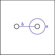
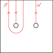
Figure 1: The closed curves $a$, $b$ and the arcs $\alpha$, $\beta$, $\alpha^{\prime}$, $\beta^{\prime}$.

7.1 Genus one

Here we consider the genus $1$ case with $n=2$ configuration points. Let $a$, $b$ be simple closed curves representing the symplectic basis of $H_{1}(\Sigma)$ previously denoted $(a_{1},b_{1})$. We will use the same notation $a$, $b$ for the curves, their homology classes and their lifts in $\mathcal{H}$ which were previously $\tilde{a}$, $\tilde{b}$. The corresponding Dehn twists are denoted by $T_{a}$, $T_{b}$. The homology $H_{2}^{BM}(\mathcal{C}_{2}(\Sigma),\mathcal{C}_{2}(\Sigma,\partial^{-}(\Sigma));\mathcal{H})$ is a free module of rank $3$ over $\mathbb{Z}[\mathcal{H}]$. A basis was described in Theorem 10. Here we replace $\gamma_{1}$, $\gamma_{2}$ by $\alpha$, $\beta$ depicted in Figure 1, and the basis is denoted by $w(\alpha)=E_{(2,0)}$, $w(\beta)=E_{(0,2)}$, $v(\alpha,\beta)=E_{(1,1)}$. In more detail, $w(\alpha)$ is represented by the cycle in the $2$-point configuration space given by the subspace where both points lie on the arc $\alpha$. Similarly, $w(\beta)$ is given by the subspace where both points lie on $\beta$ and $v(\alpha,\beta)$ is given by the subspace where exactly one point lies on each of these arcs.

In fact, we have to be even more careful to specify these elements precisely, since the preceding description only determines them up to the action of the deck transformation group $\mathcal{H}$, because we have just described cycles in the configuration space $\mathcal{C}_{2}(\Sigma)$, whereas cycles for the Heisenberg-twisted homology are cycles in the covering space $\widetilde{\mathcal{C}}_{2}(\Sigma)$. To specify such a lifting of the cycles in $\mathcal{C}_{2}(\Sigma)$ that we have described, we first choose once and for all a base configuration $c_{0}$ contained in $\partial\Sigma$ and a lift of $c_{0}$ to $\widetilde{\mathcal{C}}_{2}(\Sigma)$. A lift of a cycle to $\widetilde{\mathcal{C}}_{2}(\Sigma)$ is therefore determined by a choice of a path (called a “tether”) in $\mathcal{C}_{2}(\Sigma)$ from a point in the cycle to $c_{0}$. For $w(\alpha)$, $w(\beta)$ and $v(\alpha,\beta)$, we choose these tethers as illustrated in the top row of Figure 2.

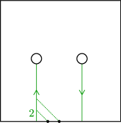
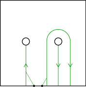
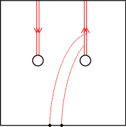
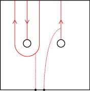
Figure 2: Tethers.

By Poincaré duality, and the fact that $\mathcal{C}_{2}(\Sigma)$ is a connected, oriented $4$-manifold with boundary $\mathcal{C}_{2}(\Sigma,\partial\Sigma)=\{c\in\mathcal{C}_{2}(\Sigma)\mid c\cap\partial\Sigma\neq\varnothing\}$, we have a non-degenerate pairing

$$\langle-,-\rangle\colon H_{2}^{BM}(\mathcal{C}_{2}(\Sigma),\partial^{-};\mathbb{Z}[\mathcal{H}])\otimes H_{2}(\mathcal{C}_{2}(\Sigma),\partial^{+};\mathbb{Z}[\mathcal{H}])\longrightarrow\mathbb{Z}[\mathcal{H}],$$ (63)

where $\partial^{\pm}$ is an abbreviation of $\mathcal{C}_{2}(\Sigma,\partial^{\pm}(\Sigma))$, and we note that the boundary $\partial\mathcal{C}_{2}(\Sigma)=\mathcal{C}_{2}(\Sigma,\partial\Sigma)$ decomposes as $\partial^{+}\cup\partial^{-}$, corresponding to the decomposition of the boundary of the surface $\partial\Sigma=\partial^{+}(\Sigma)\cup\partial^{-}(\Sigma)$. (Formally, it is a manifold triad.) There are natural elements of $H_{2}(\mathcal{C}_{2}(\Sigma),\partial^{+};\mathbb{Z}[\mathcal{H}])$ that are dual to $w(\alpha)$, $w(\beta)$ and $v(\alpha,\beta)$ with respect to this pairing, which we denote by $\overline{w}(\alpha^{\prime})$, $\overline{w}(\beta^{\prime})$ and $v(\alpha^{\prime},\beta^{\prime})$ respectively. The element $v(\alpha^{\prime},\beta^{\prime})$ is defined exactly as above: it is given by the subspace of $2$-point configurations where one point lies on each of the arcs $\alpha^{\prime}$ and $\beta^{\prime}$ of Figure 1. The element $\overline{w}(\alpha^{\prime})$ is defined as follows: first replace the arc $\alpha^{\prime}$ with two parallel copies $\alpha^{\prime}_{1}$ and $\alpha^{\prime}_{2}$ (as in the bottom-left of Figure 2), and then $\overline{w}(\alpha^{\prime})$ is given by the subspace of $2$-point configurations where one point lies on each of $\alpha^{\prime}_{1}$ and $\alpha^{\prime}_{2}$. The element $\overline{w}(\beta^{\prime})$ is defined exactly analogously. Again, in order to specify these elements precisely, we have to choose tethers, which are illustrated in the bottom row of Figure 2.

A practical description of the pairing (63) is as follows. Let $x=w(\gamma)$ or $v(\gamma,\delta)$ for disjoint arcs $\gamma$, $\delta$ with endpoints on $\partial^{-}(\Sigma)$, and choose a tether for $x$, namely a path $t_{x}$ from $c_{0}$ to a point in $x$. Similarly, let $y=\overline{w}(\epsilon)$ or $v(\epsilon,\zeta)$ for disjoint arcs $\epsilon$, $\zeta$ with endpoints on $\partial^{+}(\Sigma)$, and choose a tether $t_{y}$ for $y$. Suppose that the arcs $\gamma\sqcup\delta$ intersect the arcs $\epsilon\sqcup\zeta$ transversely. Then the pairing (63) is given by the formula

$$\bigl{\langle}[x,t_{x}],[y,t_{y}]\bigr{\rangle}=\sum_{p=\{p_{1},p_{2}\}\in x\cap y}\mathrm{sgn}(p_{1}).\mathrm{sgn}(p_{2}).\mathrm{sgn}(\ell_{p}).\phi(\ell_{p}),$$ (64)

where $\ell_{p}\in\mathbb{B}_{2}(\Sigma)$ is the loop in $\mathcal{C}_{2}(\Sigma)$ given by concatenating:

• the tether $t_{x}$ from $c_{0}$ to a point in $x$,

• a path in $x$ to the intersection point $p$,

• a path in $y$ from $p$ to the endpoint of the tether $t_{y}$,

• the reverse of the tether $t_{y}$ back to $c_{0}$,

$\mathrm{sgn}(\ell_{p})\in\{+1,-1\}$ is the sign of the induced permutation in $\mathfrak{S}_{2}$ and $\mathrm{sgn}(p_{i})\in\{+1,-1\}$ is given by the sign convention in Figure 3.

(In fact, there should be an extra global $-1$ sign on the right-hand side of (64), which we have suppressed for simplicity. Thus (64) is really a formula for $-\eqref{eq:pairing}$. This global sign ambiguity does not affect our calculations, since all we need is a non-degenerate pairing of the form (63), and any non-degenerate pairing multiplied by a unit is again a non-degenerate pairing. This extra global sign also appears in Bigelow’s formula [12, page 475, ten lines above Lemma 2.1]. See Appendix B for further explanations of these signs.)

With this description of (63), it is easy to verify that the matrix

$$\left(\begin{matrix}\langle[w(\alpha)],[\overline{w}(\alpha^{\prime})]\rangle&\langle[w(\alpha)],[\overline{w}(\beta^{\prime})]\rangle&\langle[w(\alpha)],[v(\alpha^{\prime},\beta^{\prime})]\rangle\\ \langle[w(\beta)],[\overline{w}(\alpha^{\prime})]\rangle&\langle[w(\beta)],[\overline{w}(\beta^{\prime})]\rangle&\langle[w(\beta)],[v(\alpha^{\prime},\beta^{\prime})]\rangle\\ \langle[v(\alpha,\beta)],[\overline{w}(\alpha^{\prime})]\rangle&\langle[v(\alpha,\beta)],[\overline{w}(\beta^{\prime})]\rangle&\langle[v(\alpha,\beta)],[v(\alpha^{\prime},\beta^{\prime})]\rangle\end{matrix}\right)\;\in\;\mathrm{Mat}_{3,3}(\mathbb{Z}[\mathcal{H}])$$

is the identity; this is the precise sense in which these two $3$-tuples of elements are “dual” to each other.

Figure 3: Sign convention for intersections between cycles representing elements of the homology groups $H_{n}^{BM}(\mathcal{C}_{n}(\Sigma),\partial^{-};\mathbb{Z}[\mathcal{H}])$ and $H_{n}(\mathcal{C}_{n}(\Sigma),\partial^{+};\mathbb{Z}[\mathcal{H}])$.

Theorem 44.

With respect to the ordered basis $(w(\alpha),w(\beta),v(\alpha,\beta))$:

(a) The matrix for the isomorphism

$$\mathcal{T}_{a}=\mathcal{C}_{2}(T_{a})_{*}\colon H_{2}^{BM}(\mathcal{C}_{2}(\Sigma),\partial^{-};\mathbb{Z}[\mathcal{H}])_{(T_{a}^{-1})_{\mathcal{H}}}\longrightarrow H_{2}^{BM}(\mathcal{C}_{2}(\Sigma),\partial^{-};\mathbb{Z}[\mathcal{H}])$$

is

$$M_{a}=\left(\begin{array}[]{rrr}1&u^{2}a^{-2}b^{2}&(u^{-1}-1)a^{-1}b\\ 0&1&0\\ 0&-a^{-1}b&1\end{array}\right)\ .$$

(b) The matrix for the isomorphism

$$\mathcal{T}_{b}=\mathcal{C}_{2}(T_{b})_{*}\colon H_{2}^{BM}(\mathcal{C}_{2}(\Sigma),\partial^{-};\mathbb{Z}[\mathcal{H}])_{(T_{b}^{-1})_{\mathcal{H}}}\longrightarrow H_{2}^{BM}(\mathcal{C}_{2}(\Sigma),\partial^{-};\mathbb{Z}[\mathcal{H}])$$

is

$$M_{b}=\left(\begin{array}[]{rrr}u^{-2}b^{2}&0&0\\ -u^{-1}&1&1-u^{-1}\\ -u^{-1}b&0&b\end{array}\right)\ .$$

Proof. Let us simplify the notation for the basis and the corresponding dual homology classes by

$$(e_{1},e_{2},e_{3})=(w(\alpha),w(\beta),v(\alpha,\beta))\qquad(e^{\prime}_{1},e^{\prime}_{2},e^{\prime}_{3})=(\overline{w}(\alpha^{\prime}),\overline{w}(\beta^{\prime}),v(\alpha^{\prime},\beta^{\prime})).$$

Using the non-degenerate pairing (63) and elementary linear algebra, we have that

$$\mathcal{C}_{2}(f)_{*}(e_{i})=\sum_{j=1}^{3}e_{j}.\langle\mathcal{C}_{2}(f)_{*}(e_{i}),e^{\prime}_{j}\rangle$$

for any $f\in\mathfrak{M}(\Sigma)$. Computing the matrices $M_{a}$ and $M_{b}$ therefore consists in computing $\langle\mathcal{T}_{a}(e_{i}),e^{\prime}_{j}\rangle$ and $\langle\mathcal{T}_{b}(e_{i}),e^{\prime}_{j}\rangle$ for $i,j\in\{1,2,3\}$. We will explain how to compute two of these 18 elements of $\mathbb{Z}[\mathcal{H}]$, the remaining 16 being left as exercises for the reader. In each case the idea is the same: apply the Dehn twist to the explicit cycle (described above) representing the homology class $e_{i}$, and then use the formula (64) to compute the pairing.

We begin by computing $\langle\mathcal{T}_{a}(e_{2}),e^{\prime}_{1}\rangle=\langle\mathcal{T}_{a}(w(\beta)),\overline{w}(\alpha^{\prime})\rangle$, the top-middle entry of $M_{a}$.

$$\langle\mathcal{T}_{a}(w(\beta)),\overline{w}(\alpha^{\prime})\rangle =\langle w(T_{a}(\beta)),\overline{w}(\alpha^{\prime})\rangle$$

$$=\raisebox{-0.5pt}{\includegraphics[scale={0.4}]{calc-example-1.pdf}}$$

$$=(-1).(-1).(+1).\phi\left(\;\raisebox{-0.48pt}{\includegraphics[scale={0.3}]{calc-example-1a.pdf}}\;\right)$$

$$=\phi(a^{-1}b\sigma^{-1}a^{-1}b\sigma)$$

$$=a^{-1}ba^{-1}b$$

$$=u^{2}a^{-2}b^{2}.$$

We next calculate $\langle\mathcal{T}_{a}(e_{3}),e^{\prime}_{1}\rangle=\langle\mathcal{T}_{a}(v(\alpha,\beta)),\overline{w}(\alpha^{\prime})\rangle$, the top-right entry of $M_{a}$. This is slightly more complicated, since in this case there are two intersection points in the configuration space $\mathcal{C}_{2}(\Sigma)$, so we obtain a Heisenberg polynomial (i.e. element of $\mathbb{Z}[\mathcal{H}]$) with two terms.

$$\langle\mathcal{T}_{a}(v(\alpha,\beta)),\overline{w}(\alpha^{\prime})\rangle =\langle v(\alpha,T_{a}(\beta)),\overline{w}(\alpha^{\prime})\rangle$$

$$=\raisebox{-0.5pt}{\includegraphics[scale={0.4}]{calc-example-2.pdf}}+\raisebox{-0.5pt}{\includegraphics[scale={0.4}]{calc-example-2bis.pdf}}$$

$$=(-1).(+1).(-1).\phi\left(\;\raisebox{-0.48pt}{\includegraphics[scale={0.3}]{calc-example-2a.pdf}}\;\right)$$

$$\qquad\qquad\qquad+(+1).(-1).(+1).\phi\left(\;\raisebox{-0.48pt}{\includegraphics[scale={0.3}]{calc-example-2bisa.pdf}}\;\right)$$

$$=\phi(\sigma^{-1}a^{-1}b)-\phi(a^{-1}b)$$

$$=u^{-1}a^{-1}b-a^{-1}b$$

$$=(u^{-1}-1)a^{-1}b.$$

The other 16 entries of the matrices $M_{a}$ and $M_{b}$ may be computed analogously.   

Notation 45.

To shorten the notation in the following, we will use the abbreviation

$$A\coloneqq H_{2}^{BM}(\mathcal{C}_{2}(\Sigma),\mathcal{C}_{2}(\Sigma,\partial^{-}(\Sigma));\mathcal{H})=H_{2}^{BM}(\mathcal{C}_{2}(\Sigma),\partial^{-};\mathbb{Z}[\mathcal{H}]).$$

Remark 46 (Verifying the braid relation.).

Recall that $\mathfrak{M}(\Sigma_{1,1})$ is generated by $T_{a}$ and $T_{b}$ subject to the single relation $T_{a}T_{b}T_{a}=T_{b}T_{a}T_{b}$. It must therefore be the case that the isomorphism

is equal to the isomorphism

in other words, using Lemma 43, we must have the following equality of matrices:

$$M_{a}.(T_{a})_{\mathcal{H}}(M_{b}).(T_{a}T_{b})_{\mathcal{H}}(M_{a})=M_{b}.(T_{b})_{\mathcal{H}}(M_{a}).(T_{b}T_{a})_{\mathcal{H}}(M_{b}),$$ (65)

where $M_{a}$ and $M_{b}$ are as in Theorem 44 and the automorphisms $(T_{a})_{\mathcal{H}},(T_{b})_{\mathcal{H}}\in\mathrm{Aut}(\mathcal{H})$ are extended linearly to automorphisms of $\mathbb{Z}[\mathcal{H}]$ and thus to automorphisms of matrices over $\mathbb{Z}[\mathcal{H}]$. Indeed, one may calculate that both sides of (65) are equal to

$$\left(\begin{matrix}0&u^{2}a^{-2}b^{2}&0\\ -u^{-1}&1+(u^{-3}-u^{-2})a^{-1}-u^{-5}a^{-2}&(1-u^{-1})(1+u^{-3}a^{-1})\\ 0&-a^{-1}b-u^{-1}a^{-2}b&u^{-1}a^{-1}b\end{matrix}\right).$$ (66)

Remark 47 (The Dehn twist around the boundary.).

In a similar way, we may compute the matrix $M_{\partial}$ for the action $\mathcal{T}_{\partial}$ of the Dehn twist $T_{\partial}$ around the boundary of $\Sigma_{1,1}$. We note that $T_{\partial}$ lies in the Chillingworth subgroup of $\mathfrak{M}(\Sigma_{1,1})$, so its action on $\mathcal{H}$ is trivial and the action $\mathcal{T}_{\partial}$ is an automorphism

$$\mathcal{T}_{\partial}\colon A\longrightarrow A.$$

However, to compute its matrix $M_{\partial}$, it is convenient to decompose $\mathcal{T}_{\partial}$ into isomorphisms as follows. Write $g=T_{a}T_{b}T_{a}=T_{b}T_{a}T_{b}$, so that $T_{\partial}=g^{4}$. Then $\mathcal{T}_{\partial}$ decomposes as

where $\mathcal{T}_{g}$ denotes the action of $g$, given by the matrix (66) above. The matrix $M_{\partial}$ may therefore be obtained by multiplying together four copies of (66), shifted by the actions of $\mathrm{id}$, $g_{\mathcal{H}}$, $g^{2}_{\mathcal{H}}$ and $g^{3}_{\mathcal{H}}$ respectively. This may be implemented in Sage to show that $M_{\partial}$ is equal to the matrix displayed in Figure 4. More details of these Sage calculations are given in Appendix C.

One may verify explicitly by hand that, if we set $a=b=u^{2}=1$ in the matrix $M_{\partial}=(\text{Figure \ref{fig:bigmatrix}})$, it simplifies to the identity matrix. This is expected, since applying this specialisation to our representation recovers the second Moriyama representation (as discussed in §6; see in particular the quotient (59) of $\mathfrak{M}(\Sigma)$-representations), whose kernel is the Johnson kernel $\mathfrak{J}(2)$ by [32], which contains $T_{\partial}$.

$$\left(\begin{matrix}\begin{smallmatrix}u^{-8}b^{2}+u^{-4}a^{-2}-ua^{-2}b^{2}+(u^{-1}-u^{-2})a^{-2}b+\\ (u^{-3}-u^{-4})a^{-1}b^{2}+(u^{-4}-u^{-5})a^{-1}b\end{smallmatrix}&\begin{smallmatrix}(u^{2}+1-2u^{-1}+u^{-2}+u^{-4})a^{-2}b^{2}-ua^{-2}b^{4}+\\ (-u^{2}+u+u^{-1}-u^{-2})a^{-2}b^{3}-u^{-3}a^{-2}+\\ (-1+u^{-1}+u^{-3}-u^{-4})a^{-2}b\end{smallmatrix}&\begin{smallmatrix}(-1+2u^{-1}-u^{-2}-u^{-4}+u^{-5})a^{-2}b+\\ (u-1)a^{-2}b^{3}+(u^{2}-u-u^{-1}+2u^{-2}-u^{-3})a^{-2}b^{2}+\\ (-u^{-3}+u^{-4})a^{-1}b+(u^{-4}-u^{-5})a^{-1}b^{3}+\\ (-u^{-2}+u^{-3}+u^{-5}-u^{-6})a^{-1}b^{2}+\\ (-u^{-3}+u^{-4})a^{-2}\end{smallmatrix}\\[38.74985pt] \begin{smallmatrix}-u^{-1}-u^{-3}+2u^{-4}-u^{-5}-u^{-7}+u^{-2}a^{2}+\\ (u^{-1}-u^{-2}-u^{-4}+u^{-5})a+u^{-6}a^{-2}+\\ (u^{-3}-u^{-4}-u^{-6}+u^{-7})a^{-1}\end{smallmatrix}&\begin{smallmatrix}1+u^{-2}-u^{-3}+u^{-6}+u^{-6}a^{-2}b^{2}-u^{-1}b^{2}+\\ (u^{-3}-u^{-4})a^{-1}b^{2}+(-1+u^{-1}+u^{-3}-u^{-4})b+\\ (u^{-2}-2u^{-3}+u^{-4}+u^{-6}-u^{-7})a^{-1}b-u^{-5}a^{-2}+\\ (-u^{-2}+u^{-3}+u^{-5}-u^{-6})a^{-1}+(u^{-5}-u^{-6})a^{-2}b\end{smallmatrix}&\begin{smallmatrix}(-u^{-6}+u^{-7})a^{-2}b+\\ (u^{-1}-u^{-2}-u^{-4}+2u^{-5}-u^{-6})b+\\ (-u^{-3}+2u^{-4}-u^{-5}-u^{-7}+u^{-8})a^{-1}b+\\ 1-u^{-1}+u^{-2}-3u^{-3}+2u^{-4}+u^{-6}-u^{-7}+\\ (-u^{-2}+2u^{-3}-u^{-4}+u^{-5}-2u^{-6}+u^{-7})a^{-1}\\ +(u^{-2}-u^{-3})ab+(-1+u^{-1}+u^{-3}-u^{-4})a+\\ (-u^{-5}+u^{-6})a^{-2}\end{smallmatrix}\\[38.74985pt] \begin{smallmatrix}-u^{-6}ab+(-u^{-3}+u^{-4}-u^{-7})b-u^{-4}+\\ (u^{-1}-u^{-4}+u^{-5})a^{-1}b+u^{-2}a^{-2}b+\\ (-u^{-3}+u^{-6})a^{-1}+u^{-5}a^{-2}\end{smallmatrix}&\begin{smallmatrix}(-1-u^{-2}+2u^{-3}-u^{-6})a^{-1}b+u^{-1}a^{-1}b^{3}+\\ u^{-2}a^{-2}b^{3}+(1-u^{-1}-u^{-3}+u^{-4})a^{-1}b^{2}+\\ (u^{-1}-u^{-2}+u^{-5})a^{-2}b^{2}+(-u^{-1}+u^{-4}-u^{-5})a^{-2}b+\\ (u^{-2}-u^{-5})a^{-1}-u^{-4}a^{-2}\end{smallmatrix}&\begin{smallmatrix}u^{-3}+(u^{-2}-u^{-3}-u^{-5}+u^{-6})a^{-1}+\\ (-u^{-1}+u^{-2}-u^{-5}+u^{-6})a^{-1}b^{2}+\\ (-u^{-2}+u^{-3})a^{-2}b^{2}+\\ (-1+u^{-1}+2u^{-3}-3u^{-4}+u^{-7})a^{-1}b+\\ (-u^{-1}+u^{-2}-u^{-5}+u^{-6})a^{-2}b+(-u^{-4}+u^{-5})b^{2}+\\ (u^{-2}-u^{-3}-u^{-5}+u^{-6})b+(-u^{-4}+u^{-5})a^{-2}\end{smallmatrix}\end{matrix}\right)$$

Figure 4: The action of the Dehn twist around the boundary of $\Sigma_{1,1}$.

7.2 Higher genus

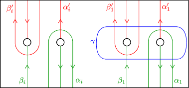
Figure 5: The arcs $\alpha_{i},\beta_{i},\alpha^{\prime}_{i},\beta^{\prime}_{i}$ and the closed genus-one-separating curve $\gamma$.

For arbitrary genus $g\geqslant 1$, we view the surface $\Sigma=\Sigma_{g,1}$ as the quotient of the punctured rectangle depicted in Figure 5, where the $2g$ holes are identified in pairs by reflection. The arcs $\alpha_{i},\beta_{i}$ for $i\in\{1,\ldots,g\}$ form a symplectic basis for the first homology of $\Sigma$ relative to the lower edge of the rectangle. Following Theorem 10, a basis for the free $\mathbb{Z}[\mathcal{H}]$-module $H_{2}^{BM}(\mathcal{C}_{2}(\Sigma),\mathcal{C}_{2}(\Sigma,\partial^{-}(\Sigma));\mathcal{H})$ is given by the homology classes represented by the $2$-cycles

• $w(\epsilon)$ for $\epsilon\in\{\alpha_{1},\beta_{1},\alpha_{2},\beta_{2},\ldots,\alpha_{g},\beta_{g}\}$,

• $v(\delta,\epsilon)$ for $\delta,\epsilon\in\{\alpha_{1},\beta_{1},\alpha_{2},\beta_{2},\ldots,\alpha_{g},\beta_{g}\}$ with $\delta<\epsilon$

where we use the ordering $\alpha_{1}<\beta_{1}<\alpha_{2}<\cdots<\alpha_{g}<\beta_{g}$. Here $w(\epsilon)$ denotes the subspace of configurations where both points lie on $\epsilon$ and $v(\delta,\epsilon)$ denotes the subspace of configurations where one point lies on each of $\delta$ and $\epsilon$. As in the genus $1$ setting, we have to be more careful to specify these elements precisely; this is done by choosing, for each of the $2$-cycles listed above, a path (called a “tether”) in $\mathcal{C}_{2}(\Sigma)$ from a point in the cycle to $c_{0}$, the base configuration, which is contained in the bottom edge of the rectangle. Note that the space of configurations of two points in the bottom edge of the rectangle is contractible, so it is equivalent to choose a path in $\mathcal{C}_{2}(\Sigma)$ from a point in the cycle to any configuration contained in the bottom edge of the rectangle.

For cycles of the form $w(\epsilon)$, we may choose tethers exactly as in the genus $1$ setting: see the top-left and top-middle of Figure 2. For cycles of the form $v(\alpha_{i},\beta_{i})$, we may also choose tethers exactly as in the genus $1$ setting: see the top-right of Figure 2. For other cycles of the form $v(\delta,\epsilon)$, we choose tethers as illustrated in Figure 6.

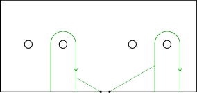
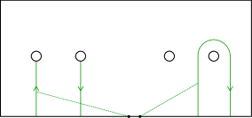
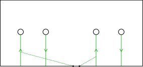
Figure 6: More tethers.

Exactly as in the genus $1$ setting, there is a non-degenerate pairing (63) defined via Poincaré duality for the $4$-manifold-with-boundary $\mathcal{C}_{2}(\Sigma)$. Associated to the collection of arcs $\alpha^{\prime}_{i},\beta^{\prime}_{i}$ illustrated in Figure 5 there are elements of $H_{2}(\mathcal{C}_{2}(\Sigma),\partial^{+};\mathcal{H})$:

• $\overline{w}(\epsilon)$ for $\epsilon\in\{\alpha^{\prime}_{1},\beta^{\prime}_{1},\alpha^{\prime}_{2},\beta^{\prime}_{2},\ldots,\alpha^{\prime}_{g},\beta^{\prime}_{g}\}$,

• $v(\delta,\epsilon)$ for $\delta,\epsilon\in\{\alpha^{\prime}_{1},\beta^{\prime}_{1},\alpha^{\prime}_{2},\beta^{\prime}_{2},\ldots,\alpha^{\prime}_{g},\beta^{\prime}_{g}\}$ with $\delta<\epsilon$

where we use the ordering $\alpha^{\prime}_{1}<\beta^{\prime}_{1}<\alpha^{\prime}_{2}<\cdots<\alpha^{\prime}_{g}<\beta^{\prime}_{g}$. Here, $\overline{w}(\epsilon)$ is the subspace of configurations where one point lies on each of $\epsilon^{+}$ and $\epsilon^{-}$, where $\epsilon^{+},\epsilon^{-}$ are two parallel, disjoint copies of $\epsilon$. As above, we specify these elements precisely by choosing tethers (paths in $\mathcal{C}_{2}(\Sigma)$ from a point on the cycle to a configurations contained in the bottom edge of the rectangle). For elements of the form $\overline{w}(\epsilon)$ or $v(\alpha^{\prime}_{i},\beta^{\prime}_{i})$, we choose these exactly as in the genus $1$ setting; see the bottom row of Figure 2. For other elements of the form $v(\delta,\epsilon)$, we choose them as illustrated in Figure 7.

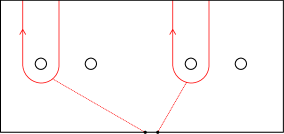
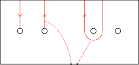
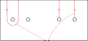
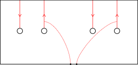
Figure 7: Even more tethers.

Remark 48.

These choices of tethers may seem a little arbitrary, and indeed they are; however, any different choice would have the effect simply of changing the chosen basis for the Heisenberg homology $H_{2}^{BM}(\mathcal{C}_{2}(\Sigma),\partial^{-};\mathcal{H})$ by rescaling each basis vector by a unit of $\mathbb{Z}[\mathcal{H}]$. This would have the effect of conjugating the matrices that we calculate by an invertible diagonal matrix.

The geometric formula (64) for the non-degenerate pairing $\langle-\mathbin{,}-\rangle$ holds exactly as in the genus $1$ setting, and one may easily verify using this formula that the bases

$$\begin{split}\mathcal{B}&=\{w(\epsilon),v(\delta,\epsilon)\mid\delta<\epsilon\in\{\alpha_{1},\ldots,\beta_{g}\}\}\\ \mathcal{B}^{\prime}&=\{\overline{w}(\epsilon),v(\delta,\epsilon)\mid\delta<\epsilon\in\{\alpha^{\prime}_{1},\ldots,\beta^{\prime}_{g}\}\}\end{split}$$ (67)

for $H_{2}^{BM}(\mathcal{C}_{2}(\Sigma),\partial^{-};\mathcal{H})$ and $H_{2}(\mathcal{C}_{2}(\Sigma),\partial^{+};\mathcal{H})$ respectively are dual with respect to this pairing. Choose a total ordering of $\mathcal{B}$ as follows:

• $w(\alpha_{1})$, $w(\beta_{1})$, $v(\alpha_{1},\beta_{1})$,

• $v(\alpha_{1},\epsilon)$ for $\epsilon=\alpha_{2},\beta_{2},\ldots,\alpha_{g},\beta_{g}$,

• $v(\beta_{1},\epsilon)$ for $\epsilon=\alpha_{2},\beta_{2},\ldots,\alpha_{g},\beta_{g}$,

• followed by all other basis elements in any order,

and similarly for $\mathcal{B}^{\prime}$. Denote by $\gamma$ the genus-$1$ separating curve in $\Sigma$ pictured in Figure 5.

Theorem 49.

With respect to the ordered bases (67), the matrix for the automorphism $\mathcal{T}_{\gamma}=\mathcal{C}_{2}(T_{\gamma})_{*}$ of $H_{2}^{BM}(\mathcal{C}_{2}(\Sigma),\partial^{-};\mathcal{H})$ is given in block form as

$$M_{\gamma}=\left(\begin{matrix}\Lambda&0&0&0\\ 0&p.I&r.I&0\\ 0&q.I&s.I&0\\ 0&0&0&I\end{matrix}\right),$$ (68)

where $\Lambda$ is the $3\times 3$ matrix depicted in Figure 4, the middle two columns and rows each have width/height $2g-2$ and the Heisenberg polynomials $p,q,r,s\in\mathbb{Z}[\mathcal{H}]$ are:

• $p=-a^{-1}b+u^{-2}b+u^{-2}a^{-1}$,

• $q=1-a+u^{-2}-u^{-2}a^{-1}$,

• $r=a^{-1}(-b+b^{2}+u^{-2}-u^{-2}b)$,

• $s=1-b+u^{-2}+u^{-2}a^{-1}b-u^{-2}a^{-1}$,

where we are abbreviating the elements $a_{1},b_{1}\in\mathcal{H}$ as $a,b$ respectively.

Proof. As in the proof of Theorem 44, this reduces to computing $\langle\mathcal{T}_{\gamma}(e_{i}),e^{\prime}_{j}\rangle$ as $e_{i}$ and $e^{\prime}_{j}$ run through the ordered bases (67).

First note that the basis elements come in three types: those entirely supported in the genus-$1$ subsurface containing $\gamma$ (the first three), those supported partially in this subsurface and partially in the complementary genus-$(g-1)$ subsurface (the next $4g-4$) and those supported entirely outside of the genus-$1$ subsurface (the rest). The Dehn twist $T_{\gamma}$ does not mix these two complementary subsurfaces, so $M_{\gamma}$ is a block matrix with respect to this partition.

The top-left $3\times 3$ matrix involves only the basis elements $w(\alpha_{1})$, $w(\beta_{1})$, $v(\alpha_{1},\beta_{1})$ and their duals, and so the calculation of this submatrix is identical to the calculation in genus $1$, which is given by the matrix in Figure 4.

The bottom-right submatrix involves only basis elements supported outside of the genus-$1$ subsurface containing $\gamma$, so the effect of $\mathcal{T}_{\gamma}$ is the identity on these elements.

It remains to calculate the middle $(4g-4)\times(4g-4)$ submatrix, which records the effect of $\mathcal{T}_{\gamma}$ on $v(\alpha_{1},\epsilon)$ and $v(\beta_{1},\epsilon)$ for $\epsilon\in\{\alpha_{2},\ldots,\beta_{g}\}$. Since $\epsilon\cap\gamma=\varnothing$, we must have

$$\mathcal{T}_{\gamma}(v(\alpha_{1},\epsilon)) =p_{\epsilon}.v(\alpha_{1},\epsilon)+q_{\epsilon}.v(\beta_{1},\epsilon)$$

$$\mathcal{T}_{\gamma}(v(\beta_{1},\epsilon)) =r_{\epsilon}.v(\alpha_{1},\epsilon)+s_{\epsilon}.v(\beta_{1},\epsilon)$$

for some $p_{\epsilon},q_{\epsilon},r_{\epsilon},s_{\epsilon}\in\mathbb{Z}[\mathcal{H}]$. Precisely, we have

$$p_{\epsilon} =\big{\langle}v(T_{\gamma}(\alpha_{1}),\epsilon),v(\alpha^{\prime}_{1},\epsilon^{\prime})\big{\rangle} q_{\epsilon} =\big{\langle}v(T_{\gamma}(\alpha_{1}),\epsilon),v(\beta^{\prime}_{1},\epsilon^{\prime})\big{\rangle}$$

$$r_{\epsilon} =\big{\langle}v(T_{\gamma}(\beta_{1}),\epsilon),v(\alpha^{\prime}_{1},\epsilon^{\prime})\big{\rangle} s_{\epsilon} =\big{\langle}v(T_{\gamma}(\beta_{1}),\epsilon),v(\beta^{\prime}_{1},\epsilon^{\prime})\big{\rangle},$$

where $\epsilon^{\prime}$ denotes the dual of $\epsilon$, and we have again used the fact that $\epsilon\cap\gamma=\varnothing$ to rewrite $\mathcal{T}_{\gamma}(v(\alpha_{1},\epsilon))=v(T_{\gamma}(\alpha_{1}),T_{\gamma}(\epsilon))=v(T_{\gamma}(\alpha_{1}),\epsilon)$ and similarly for $\mathcal{T}_{\gamma}(v(\alpha_{1},\epsilon))$. From these formulas and (64) it is clear that $p_{\epsilon},q_{\epsilon},r_{\epsilon},s_{\epsilon}$ do not in fact depend on $\epsilon$. Indeed, when computing these values of the non-degenerate pairing, we may ignore one of the two configuration points (the one that starts on the left in the base configuration and which travels via the arcs $\epsilon$ and $\epsilon^{\prime}$), since it contributes neither to the signs nor to the loops $\ell_{p}$ in the formula (64). We will compute $s_{\epsilon}=s$, leaving the computation of the other three polynomials as exercises for the reader. In the following computations, as mentioned above, we ignore one of the two configuration points, since it does not contribute anything non-trivial to the formula (64).

$$s =\langle v(T_{\gamma}(\beta_{1}),\epsilon),v(\beta^{\prime}_{1},\epsilon^{\prime})\rangle$$

$$=\phantom{+}\raisebox{-0.5pt}{\includegraphics[scale={0.4}]{calc-s.pdf}}\;\;(5\text{ intersection points: }x_{1},\ldots,x_{5})$$

$$=\phantom{+}\phi\left(\;\raisebox{-0.48pt}{\includegraphics[scale={0.3}]{calc-s1.pdf}}\;\right)-\phi\left(\;\raisebox{-0.48pt}{\includegraphics[scale={0.3}]{calc-s2.pdf}}\;\right)$$

$$\phantom{=}+\phi\left(\;\raisebox{-0.48pt}{\includegraphics[scale={0.3}]{calc-s3.pdf}}\;\right)+\phi\left(\;\raisebox{-0.48pt}{\includegraphics[scale={0.3}]{calc-s4.pdf}}\;\right)$$

$$\phantom{=}-\phi\left(\;\raisebox{-0.48pt}{\includegraphics[scale={0.3}]{calc-s5.pdf}}\;\right)$$

$$=\phi(\phantom{-})-\phi(\sigma^{-1}b^{-1}aba^{-1}bab^{-1}a^{-1}b\sigma)+\phi(\sigma^{-1}ab^{-1}a^{-1}b\sigma)$$

$$\qquad+\phi(\sigma^{-1}a^{-1}bab^{-1}a^{-1}b\sigma)-\phi(\sigma^{-1}b^{-1}a^{-1}b\sigma)$$

$$=1-b+u^{-2}+u^{-2}a^{-1}b-u^{-2}a^{-1}.\hskip 156.49014pt\rule{5.0pt}{5.0pt}$$

Appendix A: a deformation retraction through Lipschitz embeddings

Here we will prove Lemma 12. We have a model for $(\Sigma,\Gamma)$ by gluing $2g$ bands $b_{j}=[-1,1]\times[-l,l]$, $1\leqslant j\leqslant 2g$ and $4g+1$ squares $c_{\nu}=[0,1]\times[0,1]$, $0\leqslant j\leqslant 4g$ according to the identifications depicted in Figure 8. We obtain a deformation retraction $h$ which is defined on each band by the formula $h_{t}(u,v)=((1-t)u,v)$ and on each square by $h_{t}(u,v)=(u,(1-t)v)$. It remains to show that for an appropriate metric $d$ the map $h_{t}$, $0\leqslant t<1$, is a $1$-Lipschitz embedding. On each band and square we use the standard Euclidean metric. Then for points $x,y\in\Sigma$, the distance $d(x,y)$ is defined as the shortest length of a path from $x$ to $y$. It is convenient to assume that $l$ is big enough so that no shortest path can go across a handle. Then $d$ is a metric which is flat outside $4g$ boundary points where the curvature is concentrated. Then we have that $h_{t}$, $0\leqslant t<1$, is a $1$-Lipshitz embedding in each band or square from which we deduce that $h_{t}$, $0\leqslant t<1$, is globally a $1$-Lipschitz embedding.

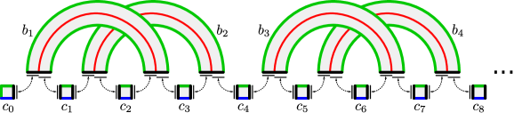
Figure 8: A model for $\Sigma$

Appendix B: signs in the intersection pairing formula

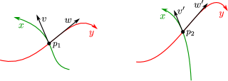
Figure 9: Choices of tangent vectors from the computation of the sign of the intersection of $x$ and $y$ at $p=\{p_{1},p_{2}\}\in\mathcal{C}_{2}(\Sigma)$.

Here we explain the signs appearing in the formula (64) for the intersection pairing on the homology of $2$-point configuration spaces, including the extra global $-1$ sign that was suppressed in (64) (see the comment in the paragraph below the formula).

We take the viewpoint that an orientation $o$ of a $d$-dimensional smooth manifold $M$ is given by a consistent choice of vector $o(p)\in\Lambda^{d}T_{p}M$ for all $p\in M$. We either choose a metric on the bundle $\Lambda^{d}TM$ and require $o(p)$ to be a unit vector with respect to this metric, or we consider $o(p)$ up to rescaling by positive real numbers.

Let us fix an orientation $o_{\Sigma}$ for the surface $\Sigma$. This determines an orientation $o_{\mathcal{C}_{2}(\Sigma)}$ of the configuration space $\mathcal{C}_{2}(\Sigma)$ by setting

$$o_{\mathcal{C}_{2}(\Sigma)}(\{p_{1},p_{2}\})=o_{\Sigma}(p_{1})\wedge o_{\Sigma}(p_{2}).$$

Recall that we have $2$-dimensional submanifolds $x$ and $y$ of $\mathcal{C}_{2}(\Sigma)$ that intersect transversely, and let $p=\{p_{1},p_{2}\}$ be a point of $x\cap y$. Let $v,w$ be the tangent vectors at $p_{1}$ and let $v^{\prime},w^{\prime}$ be the tangent vectors at $p_{2}$ illustrated in Figure 9. We have

$$v\wedge w =\mathrm{sgn}(p_{1}).o_{\Sigma}(p_{1})$$

$$v^{\prime}\wedge w^{\prime} =\mathrm{sgn}(p_{2}).o_{\Sigma}(p_{2}),$$

where $\mathrm{sgn}(p_{i})$ is the sign of the intersection of the arcs in $\Sigma$ underlying $x$ and $y$ at $p_{i}$. Similarly, we have

$$o_{x}(p)\wedge o_{y}(p)=\mathrm{sgn}(p).o_{\mathcal{C}_{2}(\Sigma)}(p),$$

where $\mathrm{sgn}(p)$ is the sign that we are trying to compute: the sign of the intersection of $x$ and $y$ in the configuration space. The orientations of $x$ and $y$ depend on the tethers $t_{x}$, $t_{y}$ that have been chosen. Precisely, we have

$$o_{x}(p) =\left\{\begin{matrix}v\wedge v^{\prime}&(*)\\ v^{\prime}\wedge v&(\dagger)\end{matrix}\right\} o_{y}(p) =\left\{\begin{matrix}w\wedge w^{\prime}&(*)\\ w^{\prime}\wedge w&(\dagger)\end{matrix}\right\},$$

where the possibilities $((*),(*))$ or $((\dagger),(\dagger))$ occur if $\mathrm{sgn}(\ell_{p})=+1$ and the possibilities $((*),(\dagger))$ or $((\dagger),(*))$ occur if $\mathrm{sgn}(\ell_{p})=-1$. We therefore have

$$o_{x}(p)\wedge o_{y}(p)=\mathrm{sgn}(\ell_{p}).(v\wedge v^{\prime})\wedge(w\wedge w^{\prime}).$$

Putting this together with the formulas above, we obtain

$$(v\wedge w)\wedge(v^{\prime}\wedge w^{\prime}) =\mathrm{sgn}(p_{1}).\mathrm{sgn}(p_{2}).o_{\Sigma}(p_{1})\wedge o_{\Sigma}(p_{2})$$

$$=\mathrm{sgn}(p_{1}).\mathrm{sgn}(p_{2}).o_{\mathcal{C}_{2}(\Sigma)}(p)$$

$$=\mathrm{sgn}(p_{1}).\mathrm{sgn}(p_{2}).\mathrm{sgn}(p).o_{x}(p)\wedge o_{y}(p)$$

$$=\mathrm{sgn}(p_{1}).\mathrm{sgn}(p_{2}).\mathrm{sgn}(p).\mathrm{sgn}(\ell_{p}).(v\wedge v^{\prime})\wedge(w\wedge w^{\prime})$$

$$=-\mathrm{sgn}(p_{1}).\mathrm{sgn}(p_{2}).\mathrm{sgn}(p).\mathrm{sgn}(\ell_{p}).(v\wedge w)\wedge(v^{\prime}\wedge w^{\prime}),$$

and hence we have

$$\mathrm{sgn}(p)=-\mathrm{sgn}(p_{1}).\mathrm{sgn}(p_{2}).\mathrm{sgn}(\ell_{p}).$$

Appendix C: Sage computations

Here we give the worksheet of the Sage computations used in the calculation of the matrix $M_{\partial}$ displayed in Figure 4 (cf. Remark 47 on page 47).

See pages - of HeisenbergAction1.pdf

References

- [1] Byung Hee An and Ki Hyoung Ko. A family of representations of braid groups on surfaces. Pacific J. Math., 247(2):257–282, 2010.
- [2] Cristina A.-M. Anghel and Martin Palmer. Lawrence-Bigelow representations, bases and duality. ArXiv:2011.02388.
- [3] Paolo Bellingeri. On presentations of surface braid groups. J. Algebra, 274(2):543–563, 2004.
- [4] Paolo Bellingeri, Sylvain Gervais, and John Guaschi. Lower central series of Artin-Tits and surface braid groups. J. Algebra, 319(4):1409–1427, 2008.
- [5] Paolo Bellingeri and Eddy Godelle. Positive presentations of surface braid groups. J. Knot Theory Ramifications, 16(9):1219–1233, 2007.
- [6] Paolo Bellingeri, Eddy Godelle, and John Guaschi. Exact sequences, lower central series and representations of surface braid groups. ArXiv:1106.4982.
- [7] Paolo Bellingeri, Eddy Godelle, and John Guaschi. Abelian and metabelian quotient groups of surface braid groups. Glasg. Math. J., 59(1):119–142, 2017.
- [8] Andrea Bianchi. Splitting of the homology of the punctured mapping class group. J. Topol., 13(3):1230–1260, 2020.
- [9] Andrea Bianchi, Jeremy Miller, and Jennifer C. H. Wilson. Mapping class group actions on configuration spaces and the Johnson filtration. ArXiv:2104.09253.
- [10] Andrea Bianchi and Andreas Stavrou. Non-trivial action of the Johnson filtration on the homology of configuration spaces. ArXiv:2208.01608.
- [11] Stephen Bigelow. Homological representations of the Iwahori-Hecke algebra. In Proceedings of the Casson Fest, volume 7 of Geom. Topol. Monogr., pages 493–507. Geom. Topol. Publ., Coventry, 2004.
- [12] Stephen J. Bigelow. Braid groups are linear. J. Amer. Math. Soc., 14(2):471–486, 2001.
- [13] Stephen J. Bigelow and Ryan D. Budney. The mapping class group of a genus two surface is linear. Algebr. Geom. Topol., 1:699–708, 2001.
- [14] M. Crivelli, G. Felder, and C. Wieczerkowski. Generalized hypergeometric functions on the torus and the adjoint representation of . Comm. Math. Phys., 154(1):1–23, 1993.
- [15] M. Crivelli, G. Felder, and C. Wieczerkowski. Topological representations of on the torus and the mapping class group. Lett. Math. Phys., 30(1):71–85, 1994.
- [16] Jacques Darné, Martin Palmer, and Arthur Soulié. When the lower central series stops: a comprehensive study for braid groups and their relatives. ArXiv:2201.03542. To appear in the Memoirs of the American Mathematical Society.
- [17] James F. Davis and Paul Kirk. Lecture notes in algebraic topology, volume 35 of Graduate Studies in Mathematics. American Mathematical Society, Providence, RI, 2001.
- [18] Florian Deloup. Topological Quantum Field Theory, Reciprocity and the Weil representation. Preliminary version.
- [19] Răzvan Gelca. Theta functions and knots. World Scientific Publishing Co. Pte. Ltd., Hackensack, NJ, 2014.
- [20] Răzvan Gelca and Alastair Hamilton. The topological quantum field theory of Riemann’s theta functions. J. Geom. Phys., 98:242–261, 2015.
- [21] Răzvan Gelca and Alejandro Uribe. From classical theta functions to topological quantum field theory. In The influence of Solomon Lefschetz in geometry and topology, volume 621 of Contemp. Math., pages 35–68. Amer. Math. Soc., Providence, RI, 2014.
- [22] Răzvan Gelca and Alejandro Uribe. Quantum mechanics and nonabelian theta functions for the gauge group . Fund. Math., 228(2):97–137, 2015.
- [23] John L. Harer. Stability of the homology of the mapping class groups of orientable surfaces. Ann. of Math. (2), 121(2):215–249, 1985.
- [24] Allen Hatcher. Algebraic topology. Cambridge University Press, Cambridge, 2002.
- [25] Derek F. Holt, Bettina Eick, and Eamonn A. O’Brien. Handbook of computational group theory. Discrete Mathematics and its Applications (Boca Raton). Chapman & Hall/CRC, Boca Raton, FL, 2005.
- [26] Dennis Johnson. A survey of the Torelli group. In Low-dimensional topology (San Francisco, Calif., 1981), volume 20 of Contemp. Math., pages 165–179. Amer. Math. Soc., Providence, RI, 1983.
- [27] Daan Krammer. Braid groups are linear. Ann. of Math. (2), 155(1):131–156, 2002.
- [28] R. J. Lawrence. Homological representations of the Hecke algebra. Comm. Math. Phys., 135(1):141–191, 1990.
- [29] Gérard Lion and Michèle Vergne. The Weil representation, Maslov index and theta series, volume 6 of Progress in Mathematics. Birkhäuser, Boston, Mass., 1980.
- [30] Jules Martel. A homological model for Verma modules and their braid representations. Geom. Topol., 26(3):1225–1289, 2022.
- [31] Shigeyuki Morita. Families of Jacobian manifolds and characteristic classes of surface bundles. I. Ann. Inst. Fourier (Grenoble), 39(3):777–810, 1989.
- [32] Tetsuhiro Moriyama. The mapping class group action on the homology of the configuration spaces of surfaces. J. Lond. Math. Soc. (2), 76(2):451–466, 2007.
- [33] Martin Palmer and Arthur Soulié. On the kernels of Moriyama-type representations of the mapping class groups. In preparation.
- [34] Andreas Stavrou. Cohomology of configuration spaces of surfaces as mapping class group representations. ArXiv:2107.08462.
- [35] Masaaki Suzuki. Irreducible decomposition of the Magnus representation of the Torelli group. Bull. Austral. Math. Soc., 67(1):1–14, 2003.
- [36] Masaaki Suzuki. Geometric interpretation of the Magnus representation of the mapping class group. Kobe J. Math., 22(1-2):39–47, 2005.
- [37] Nathalie Wahl. Homological stability for mapping class groups of surfaces. In Handbook of moduli. Vol. III, volume 26 of Adv. Lect. Math. (ALM), pages 547–583. Int. Press, Somerville, MA, 2013.