Orbit evolution in growing stellar bars: Bar-supporting orbits at the vertical ILR region

Abstract

We investigate the evolution of orbital shapes at the Inner Lindblad Resonance region of a rotating three-dimensional bar, the mass of which is growing with time. We evaluate in time-dependent models, during a 5 Gyr period, the importance of orbits with initial conditions known to play a significant role in supporting peanut-like structures in autonomous systems. These orbits are the central family of periodic orbits (x1) and vertical perturbations of it, orbits of its standard three-dimensional bifurcations at the region (x1v1 and x1v2), as well as orbits in their neighbourhood. The knowledge of the regular or chaotic character of these orbits is essential as well, because it allows us to estimate their contribution to the support of a rotating bar and, more importantly, the dynamical mechanisms that make it possible. This is calculated by means of the GALI₂ index. We find that orbital patterns existing in the autonomous case, persist for longer times in the more massive bar models, and even more so in a model in which the central spheroid component of our adopted galactic potential becomes rather insignificant. The peanut-supporting orbits which we find, have a regular or, in most cases, a weakly chaotic character. There are cases in which orbits starting close to unstable periodic orbits in an autonomous model behave as regular and support the bar when its mass increases with time. As a rule of thumb for the orbital dynamics of our non-autonomous models at a certain time, can be considered the dynamics of the corresponding frozen systems around that time.

1 Introduction

1.1 Background

Over the years we have a fairly good understanding of the orbital dynamics in rotating ellipsoids that model galactic bars. The potentials in this kind of models do not change in time, thus in order to study them, the formalism of autonomous Hamiltonian systems has been adopted (see e.g. Contopoulos & Papayannopoulos, 1980; Athanassoula et al., 1983; Contopoulos & Grosbøl, 1989; Pfenniger, 1984; Contopoulos & Magnenat, 1985; Patsis, 2005; Skokos et al., 2002a; Patsis & Athanassoula, 2019).

In all the above studies, the main mechanism reinforcing the bar, is the trapping of quasi-periodic orbits around stable periodic ones. In two-dimensional systems, these stable periodic orbits are the elliptical-like members of the x1 family (see e.g. Contopoulos & Grosbøl, 1989), while in three-dimensional models they are the stable periodic orbits of the x1-tree (Skokos et al., 2002a). According to the theory of dynamical systems, around a stable periodic orbit there is a volume in phase space, where motion is regular, i.e. the orbits will be quasi-periodic. In such a case, a particle following a quasi-periodic orbit, will remain in the neighbourhood of the periodic orbit reinforcing in this way the local density (see e.g Contopoulos, 2004, sections 2.4 and 2.5).

Nevertheless, not every quasi-periodic orbit in a model is bar-supporting. For this, it has to enhance locally the density in such a way, as to reinforce the morphological feature to be modeled, i.e. in our case the bar. A known counterexample is the case of the nearly circular retrograde orbits of the family x4, which remain stable for almost all Jaccobi constants in standard barred galaxy models (see e.g. Contopoulos & Papayannopoulos, 1980). Such orbits, if populated, would lead to the appearance of sizable counter-rotating discs at the centers of the bars, which are not observed. Most importantly there is the class of weakly chaotic and sticky chaotic orbits (Contopoulos & Harsoula, 2008), which during a certain time, may also enhance a particular bar structure (Patsis et al., 1997). As a result the bar-supporting regions on a Poincaré surface of section, do not necessarily correspond to those occupied by stability islands. The topologies of the regular and bar-supporting regions do not coincide (Chatzopoulos et al., 2011).

The next step is to examine what a time dependence of the potential may cause in the orbital dynamics of barred galaxy models. A slow variation of the gravitational field is encountered during the evolution of several $N$-body models, which simulate galactic bars (see e.g. Athanassoula, 2003; Harsoula & Kalapotharakos, 2009). “Slow”, means that the test particles have at least enough time to feel resonances (radial and vertical), the location of which does not change considerably on the galactic disks, over the time we consider. In the above mentioned work the variation of the potential between snapshots with a time distance of a few Gyr has been found to be small, so that the evolution of the model during this period could reliably be approximated by a stationary mean gravitational field.

In Manos & Machado (2014) and Machado & Manos (2016), the evolution of an $N$-body simulation of a disc galaxy within a live halo (Machado & Athanassoula, 2010), which results to the formation of a strong bar, has been approximated by means of a time-dependent (TD) analytical model. This TD model was composed of three components, namely a bar, a disc and a halo. After the initial formation of a bar, there is a relative fast increase of its size and strength, before the model enters a phase of slower variation of the parameters of its components.

In the present work we focus in the vertical Inner Lindblad Resonance (vILR) region of rotating bars. This region is either very close to, or practically identical with, the radial Inner Lindblad Resonance (rILR) region in many $N$-body, or analytic models (e.g. Combes et al., 1990; Patsis & Katsanikas, 2014a, b). We will refer to it altogether as the “ILR region”. In principle the ILR region combines orbital content that could support the thin and the thick part of the bar.

The goal of this study is to find out whether or not time variation of the potential changes significantly the orbital content of the model. This would mean that the observed structure of the boxy-peanut (hereafter b/p) bulge would be supported by totally different orbits than the known ones associated with x1 and its three-dimensional (3D) bifurcations (Skokos et al., 2002a, b; Patsis et al., 2002; Patsis & Katsanikas, 2014a, b; Patsis & Harsoula, 2018). In addition, we want to investigate whether specific orbits that support the bar in a time-independent (TI) model remain “bar-supporting”, when a parameter like the mass of the bar ($M_{B}$) varies.

1.2 Quantifying the chaoticity of the orbits

Since the reinforcement of specific structures in TI potentials is associated either with order or, under certain conditions, with weak chaos and stickiness (Contopoulos & Harsoula, 2008), it is important to know how regular or chaotic are the bar-supporting orbits in our models. To estimate this, we use the GALI₂ index (Skokos et al., 2007, 2008; Manos et al., 2012; Moges et al., 2020). The results have been compared with those obtained for the same reason with the Maximal Lyapunov Exponent (MLE) (Benettin et al., 1980a, b; Skokos, 2010) of the orbits.

The GALI₂ index is given by the norm of the wedge product of two normalized to unity deviation vectors $\mathbf{\hat{w}}_{1}(t)$ and $\mathbf{\hat{w}}_{2}(t)$ from the studied orbit, i.e. $\rm{GALI}_{2}(t)=\|\mathbf{\hat{w}}_{1}(t)\wedge\mathbf{\hat{w}}_{2}(t)\|.$ The initial coordinates, of the deviations vectors are chosen randomly, and the two vectors are orthonormalized at the beginning of the integration, setting in this way the initial value of the index to $\mbox{GALI}_{2}(0)=1$. Thus, in order to evaluate GALI₂ we simultaneously integrate the equations of motion and the so-called variational equations (see e.g. Skokos, 2010), which govern the evolution of the two deviation vectors.

Let us briefly recall the behavior of the GALI₂ index (see Skokos & Manos, 2016, and references therein). For chaotic orbits the index falls exponentially fast to zero as $\mbox{GALI}_{2}(t)\propto\exp{(-(\lambda_{1}-\lambda_{2})t)}$, where $\lambda_{1}$ and $\lambda_{2}$ are the two largest Lyapunov exponents (for the definitions and for the computation of the Lyapunov exponents see e.g. Benettin et al., 1980a, b; Skokos, 2010). On the other hand, for regular orbits it oscillates around a positive value across the integration, i.e. $\mbox{GALI}_{2}(t)\propto\mbox{constant}$. In the case of weakly chaotic or sticky orbits we observe a transition from practically constant GALI₂ values, which correspond to the seemingly quasiperiodic epoch of the orbit, to an exponential decay to zero, which indicates the orbit’s transition to chaoticity.

Orbits in TI Hamiltonian systems are either regular or chaotic, which means that their $\mbox{GALI}_{2}$ values will, respectively, oscillate around a constant positive number or eventually become zero. On the other hand orbits in TD potentials can exhibit more complicated behaviours as transitions between regular and chaotic epochs in their evolution can be observed, depending on their location in the changing phase space of the system. We use $\mbox{GALI}_{2}$ to capture these dynamical changes of orbits in TD Hamiltonians by applying the following procedure: Whenever $\mbox{GALI}_{2}$ reaches a very small value (namely when $\mbox{GALI}_{2}\leq 10^{-8}$) we reinitialize its computation by taking again two new random orthonormal deviation vectors (i.e. setting anew $\mbox{GALI}_{2}=1$) and then let these vectors evolve under the current dynamics. Since an exponential decrease of $\mbox{GALI}_{2}$ indicates chaotic behaviour, successive and frequent reinitializations of the index identify chaotic epochs, while extended periods of time where $\mbox{GALI}_{2}>10^{-8}$, correspond to a regular behaviour (Manos et al., 2013; Manos & Machado, 2014).

In order to achieve the goals of our study we proceed as follows: We consider a time interval of 5 Gyr, within which we perform our calculations. This is about half the age of a Milky-Way-type galaxy. For this period we integrate and characterize the orbits according to their chaoticity indices, as the bar mass increases linearly in time from M_Bmin to M_Bmax. We do so with a number of characteristic orbits, which we know in advance that play a key role in supporting bars in TI potentials, i.e. orbits associated with the families of the x1-tree (Skokos et al., 2002a). We check if they continue to support the initial bar structure as they evolve, if they support a similar structure with different dimensions, if they destroy the bar, or if they are transformed to other orbital shapes. In the latter case, we check also if the new orbital shapes can be identified with known patterns encountered in the phase space of TI systems. A significant factor that determines the morphological evolution of each orbit is the rate of variation of the TD parameter. For this purpose, we study for each considered case the orbital evolution in a fast and in a slowly evolving potential.

In Section 2, we describe the models we use, in Section 3 we study the behaviour of orbits in a potential with a relatively low mass bar, while in Section 4 we present the results of the corresponding study in a more massive bar model. In Section 5, we investigate the behaviour of orbits in a special case, in which the evolution of the orbital stability of the main 3D families of periodic orbits (POs) at the ILR region do not have complex unstable (for a definition see e.g. Skokos et al., 2002a) parts. Finally in Section 6 we present and discuss our conclusions.

2 The set-up of the models

A 3D autonomous Hamiltonian system describing the dynamics of a disc galaxy with a rotating bar can be written, in Cartesian coordinates $(x,y,z)$, in the form:

$$H=\frac{1}{2}(p_{x}^{2}+p_{y}^{2}+p_{z}^{2})+\Phi(x,y,z)-\Omega_{b}(xp_{y}-yp_{x}),$$ (1)

where $p_{x},~{}p_{y},$ and $p_{z}$ are the canonically conjugate momenta, $\Phi$ the gravitational potential of the model and $\Omega_{b}$ the angular velocity of the system, in our case the pattern speed of the bar. The numerical value of the Hamiltonian, E_J (Jacobi constant), is constant and we will also refer to it throughout the paper as the “energy”.

For the sake of continuity with our previous studies on the subject, we use again in this paper the popular triaxial Ferrers bar model (Ferrers, 1877), which is described in detail in Skokos et al. (2002a) and Patsis & Katsanikas (2014a), with parameters close to those in the pioneer paper by Pfenniger (1984). The formulae for the axisymmetric part of the potential, as well as the bar model, can be found in these references.

The Ferrers bar is inhomogeneous, with index 2 and axial ratios $a:b:c=6:1.5:0.6$ (with $a$, $b$, $c$ being the semi-axes). We have taken as major axis the $y-$axis. For our orbital calculations, i.e. for finding the periodic orbits and calculating Poincaré surfaces of sections (Poincaré, 1899), we consider upwards intersections with the y=0 plane. The axisymmetric background consists of a Miyamoto disc (Miyamoto & Nagai, 1975) with fixed horizontal and vertical scale lengths A=3 and B=1 respectively and a Plummer sphere (Plummer, 1911) representing the bulge, with scale length $\epsilon_{s}=0.4$. The length unit is taken as 1 kpc, the time unit as 1 Myr and the mass unit as $2\times 10^{11}M_{\odot}$.

The masses of the three components satisfy $G(M_{D}+M_{S}+M_{B})=1$, where $M_{D}$ is the total mass of the disc, $M_{S}$ the mass of the bulge (spheroid), $M_{B}$ is the mass of the bar component and $G$ the gravitational constant. We note that in our simulations the bar mass increases at the expense of the disk mass, i.e. the term $GM{{}_{D}}$ decreases appropriately so that the condition $G(M_{D}+M_{S}+M_{B})=1$ is always satisfied. An explicit halo component is not included, since our study refers to the inner parts of the galaxy, where it is considered to be not important.

We investigate the orbital evolution in the following three models, aiming to cover some typical and representative cases:

1. Model A: A bar model, in which $GM_{B}=0.05$, i.e. a relatively low mass bar, and $GM_{S}=0.08$. In this model, the variation with E_J of the stability of the main simple periodic families encountered in 3D rotating bars, i.e. x1, x1v1 and x1v2, is typical for this kind of systems (Skokos et al., 2002a).

2. Model B: A more massive bar model, with $GM_{B}=0.13$ and $GM_{S}=0.08$, in which we have again the usual variation of the stability indices of the three families.

3. Model C: A model in which the x1v1 family has no complex unstable parts (see section 3.1.1 below), all the way to corotation. In this case $GM_{B}=0.1$ and $GM_{S}=0.022$.

For all three models we follow the same steps, namely, we first investigate the behaviour of the model in the autonomous case. Then, based on the topology of the phase space at properly chosen energies, we follow the evolution of selected orbits as the mass of the bar varies. These orbits have been found to play a major role in supporting the b/p component in TI, rotating barred potentials. The criterion for choosing the initial energy of the orbits in each model, is to be in the ILR region, just beyond the critical E_J value for which the x1, x1v1 and x1v2 families are already present in the system. This procedure will be described in more detail in model A and will be repeated for models B and C.

3 Model A: A low mass bar

3.1 The autonomous case

Our goal is to investigate the orbital evolution in galactic bars as the mass of the bar increases from a M_Bmin to a M_Bmax value. To this end, we have first chosen a model in which a low mass bar is already present. The morphology of the POs at a given energy, is determined by the presence of the radial and vertical resonances (Skokos et al., 2002a). Such resonances exist in any model of a rotating 3D potential. Nevertheless, in the case of a model of a galactic bar, the influence of the bar on the dynamics of the disc has to be conspicuous and affect significantly the shape of the bar-supporting orbits. Therefore, in our model A, we have chosen $GM_{D}=$0.87$,GM_{S}$=0.08 and $GM_{B}$=0.05, which corresponds to a low mass bar. Following Skokos et al. (2002a), we have chosen $\Omega_{b}=0.054$, which places the Lagrangian points L1 and L2 at a radius of about 6.38 kpc.

3.1.1 The stability diagram

A tool for describing the dynamics of 3D Hamiltonian systems is the stability diagram (Contopoulos & Magnenat, 1985). It describes the evolution of the linear stability of families of POs, as one parameter (in our case E_J ​) varies and indicates the critical energies, at which new bifurcating families are introduced in the system (for details see Contopoulos, 2004, §2.11).

The linear stability of POs is calculated by means of the method of Broucke (1969). Details about the algorithm can be found e.g. in Contopoulos & Magnenat (1985) (see also Skokos, 2001). Here, we only mention that the variation of the stability with E_J is characterized by the variation of two stability indices, b1 and b2, one of which refers to radial and the other to vertical perturbations. A PO is stable (S) if both bi$\,\in(-2,2)$, with $i=1,2$. If one of the two stability indices is $|$bi$|>2$, then the orbit is characterized as simple unstable (U), while if both indices are $|$bi$|>2$ it is called double unstable (DU). Finally, if all four eigenvalues of the monodromy matrix are complex numbers off the unit circle, the stability indices cannot be defined and the PO is called complex unstable $(\Delta)$.

In Fig. 1 the stability curves of the x1 family are black, those of x1v1 red and of x1v2 green. Index b1 is the one associated with the radial and b2 with the vertical perturbations. The x1 family has a typical variation of the stability indices (Skokos et al., 2002a), with the b2 index having the standard “S$\rightarrow$ U$\rightarrow$ S” transition at the vILR region, bifurcating x1v1 as S and x1v2 as U, at E_J $=-0.317$ and E_J $=-0.297$, respectively. Beyond its bifurcating point, towards larger E_J ​​, x1v1 has two successive “S $\rightarrow\Delta\rightarrow$ S” transitions. As we observe in Fig. 1, this has as a consequence the presence of two $\Delta$ intervals, for $-0.303<$E_J ​$<-0.293$ and $-0.267<$E_J ​$<-0.232$. The variation of the stability indices in the autonomous case shown in Fig. 1, essentially determines the appropriate energy at which we have to start our orbital explorations in the models with parameters varying in time. In model A, we have chosen that energy to be E_J =$-0.295$ (denoted by the vertical blue line), since at this value the families x1, x1v1 and x1v2 coexist. Their representatives are S (x1), $\Delta$ (x1v1) and U (x1v2). These families of simple-periodic orbits are considered to be the most important building blocks of the boxy bulges in autonomous models (Patsis et al., 2002).

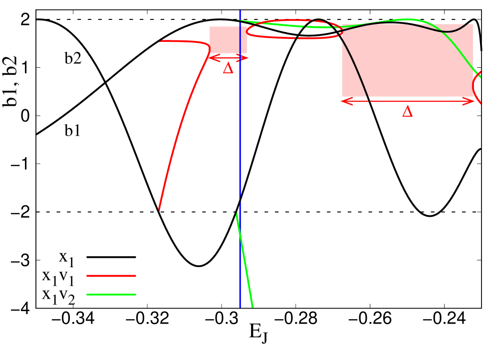
Figure 1: TI model A. Stability curves of the x1 (black curves, b1 and b2 are respectively related to radial and vertical perturbations), x1v1 (red curves) and x1v2 (green curves). The pink-shaded areas indicated by double edged arrows and by the symbol $\Delta$, denote energy ($\mbox{E}_{J}$) intervals, where x1v1 is complex unstable. The horizontal dashed lines denote the critical values -2 and 2 of the stability indices, while the vertical blue line indicates the energy value E_J =-0.295, at which we start our orbital calculations in the TD models.

3.1.2 Navigation in Phase Space

Periodic orbits determine the orbital content that supports observed morphological features in dynamical systems like the TI galactic models, since they determine the topology of the phase space. Around any stable PO exist stability tori, while the presence of unstable PO introduces chaos (see e.g. Contopoulos, 2004, chapter 2). In 2D systems, when the initial conditions (ICs) of a PO are perturbed, we can directly observe on a 2D surface of section if the displaced ICs belong to a stability island or to a chaotic zone. Then, by integrating the displaced ICs of the PO, within a pre-defined time interval, we also know if it is bar-supporting or not.

In 3D Hamiltonian systems, the 6D phase space can be reduced to a 4D space for the “surfaces” of section and for the arrays of the ICs that uniquely determine a PO (see e.g. Skokos et al., 2002a). Having the bar along the y-axis and considering the $y=0$ plane as our surface of section, the coordinates of our 4D spaces are $(x,z,p_{x},p_{z})$. We always will refer throughout the text to ICs of orbits in our system by giving the numerical values of their coordinates in this array. The visualization of such 4D surfaces of section is not trivial. A method that led to the association of specific structures in the neighbourhood of stable POs, as well as in the neighbourhood of the various kinds of unstable POs encountered in 3D Hamiltonian systems, has been introduced by Patsis & Zachilas (1994) and successfully applied in galactic models by Katsanikas & Patsis (2011); Katsanikas et al. (2011) and Katsanikas et al. (2013). However, a global visualization of the entire phase space, in which several regular and chaotic orbits coexist, has additional technical difficulties, although attempts toward this goal have already been done (Richter et al., 2014; Lange et al., 2014; Onken et al., 2016). Thus, unlike what happens in the case of the 2D surfaces of section, in the 4D spaces of section it is not straightforward to actually observe if a perturbation of the ICs of a stable, for instance, PO will lead to an orbit on an invariant torus of the same orbit, to an orbit in a chaotic sea, or even on an invariant torus of another stable PO. In this task we are still essentially blind and only by experience one can follow some interesting paths. As we will see below, in non-autonomous systems the complexity of the situation increases.

In order to detect possible candidates of orbits that support the bar morphology in TD models, we first study the phase space structure of the autonomous case and use it as a basis in our further investigations. We use 2D, $(x,p_{x})$, surfaces of section on the equatorial plane around the main family x1, as well as the $(z,p_{z})$ projections of the 4D space of section, in which the orbits are integrated for time $t=5$ Gyr. This latter projection has been proven especially helpful, because within a properly chosen integration time, the resulting figure resembles a surface of section of a 2D case. This allows us to trace directions, along which we can reach orbits in the ILR region that can be used for building a rotating bar (see e.g. Figure 14 in Patsis & Katsanikas, 2014a).

For our “starting-point” in model A, at E_J =$-0.295$, such surfaces of section are depicted in Fig. 2. The usefulness of such diagrams in identifying b/p-supporting orbits will become evident below. The main POs in the two panels are x1 (S), with initial conditions $(x_{0},z_{0},p_{x_{0}},p_{z_{0}})\approx(0.213,0,0,0)$, x1v1 $(\Delta)$ with initial conditions about $(0.213,0.253,0,0)$ and x1v2 (U) with initial conditions about $(0.211,0,0,0.059)$.

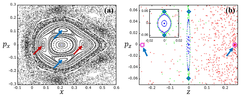
Figure 2: TI model A for E_J =-0.295. (a) The $(x,p_{x})$ surface of section around x1, located at the center of the innermost stability island. Arrows point to the four islands of the two POs of multiplicity 2, rm21 (red) and rm22 (blue) (b) The $(z,p_{z})$ projection of the Poincaré section around x1. Open circle symbols indicate the locations of x1v1 (right) and x1v1^′ (left), while the location of x1v2 ($p_{z}>0$) and x1v2^′ ($p_{z}<0$) are indicated with “diamonds”. Red points correspond to a perturbation of the x1v1 PO and they are mainly concentrated in the right-hand side of the figure. The blue points around x1 correspond to perturbed orbits lying on tori around x1 in the 4D space, while the green points belong to a perturbation of the x1v2 PO (see also embedded frame).

In the $(x,p_{x})$ surface of section in Fig. 2a, the x1 family, being stable, is at the center of the main stability island (blue dot). The central region around x1 is flanked by two sets of two islands (indicated with red and blue arrows) of the known 2-periodic families rm21 and rm22 (for the origin of these families see Patsis & Athanassoula, 2019). For orbits on the equatorial plane, surfaces of section like the one in Fig. 2a allow us to find out the morphology of any orbit displaced by $x$ or $p_{x}$ from x1, simply by integrating its ICs.

In Fig. 2b we give a $(z,p_{z}$) projection of the 4D surface of section. It includes the main POs, as well as orbits in their neighbourhood and outlines the basic structure of the phase space. Fig. 2 helps us finding orbits that potentially sustain the 3D bar, as well as the dynamical mechanisms that are in action. We observe that the stable x1 at (0,0) has the, expected, tori around it. Orbits on these tori give the blue consequents along elliptical curves around x1, resembling in this particular projection, the invariant curves we encounter in 2D surfaces of section.

The two blue “invariant curves” belong to two orbits with ICs $(0.212...,0,0,0.015)$ and $(0.212...,0,0,0.045)$. They are better viewed in the embedded frame, in the upper left corner of Fig. 2b, where the area around x1 is depicted with a different scaling of the axes. The POs x1v1 ($z>0$) and x1v1^′ ($z<0$), known in the relevant literature as “frown”-“smile” pairs, are located at the centers of the drawn open circle symbols and are also denoted by arrows, close to the left and right sides of the frame of Fig. 2b, at $p_{x}=0$. A nearby to the $(\Delta)$ x1v1 orbit with ICs (0.25,0.253…,0,0), i.e. perturbed in the x-direction, is depicted with red points. These consequents appear scattered mainly to the right of the x1 “stability island” and only a few of them are observed in the left side. The consequents corresponding to integration time of around 1 Gyr, would appear even more concentrated around the x1v1 initial conditions. The location of the U representatives of the families x1v2 ($p_{z}>0$) and x1v2^′ ($p_{z}<0$) are indicated with diamond ($\Diamond$) symbols. The plotted orbit at the immediate neighbourhood of x1v2 (green points) has ICs $(0.215,0,0,0.059...)$. Due to the proximity of the ICs of this orbit to those of the unstable periodic one and to the last torus of x1, the green consequents stick initially to the x1 “island” before they drift away into a chaotic sea.

3.1.3 Orbital morphology and stability

We have to keep in mind the following features of the main types of bar-supporting orbits, which we calculated in the autonomous model for the comparisons that will follow:

• Orbits in the x1 neighborhood: The blue invariant-like curves around x1 in Fig. 2b belong to orbits we found by perturbing its $p_{z}$ IC. We note that their side-on projections reinforce an “$\infty$”-like morphology, which becomes more striking as they approach the ICs of x1v2 (Patsis & Katsanikas, 2014a). In a way, we can say that these orbits are associated morphologically with the U PO x1v2. A regular, vertically perturbed x1 orbit, very close to x1v2, with ICs $(0.212...,0,0,0.05)$, is given in Fig. 3a. The orbit does not change essentially shape during the integration period. The three panels correspond (from left to right) to projections in the $(x,y)$, $(x,z)$ and $(y,z)$ planes, which, with respect to the bar, correspond to the face-on, end-on and side-on projections. The orbits in each individual window are coloured according to time, from red (at the beginning of the integration) to light blue (at the end of the integration), as indicated by the colour bar above the three frames

• Orbits in the x1v1 neighborhood: We found orbits close to the $\Delta$ x1v1 PO, which reinforce a boxy side-on view for considerably long times. We give in Fig. 3b a perturbed by $\Delta x$, x1v1 orbit with ICs (0.25,0.253..,0,0). In this and all subsequent similar figures, if not otherwise indicated, the orbits are presented in three successive rows, which give the evolution from top to bottom, of the face-on, end-on and side-on projections. The morphology of each orbit is depicted in each row in four successive time windows; from left to right: $0\leq t\leq 1.25$ Gyr, $1.25<t\leq 2.5$ Gyr, $2.5<t\leq 3.75$ Gyr and $3.75<t\leq 5$ Gyr. The colour bar indicating the evolution of the orbit in time, is given in this and all subsequent similar figures, at the right-hand side of each panel.

  The orbit in Fig. 3b, has a boxy shape in its face-on projection (upper row) and reinforces a boxy morphology in the side-on view for 3.75 Gyr (three first panels of the third row). For $t>3.75$ Gyr, the enhancement of boxiness is less evident. The variation of GALI₂ and MLE in the two elongated, panels at the bottom of Fig. 3b, indicates the weakly chaotic nature of the orbit. We observe that its GALI₂ requires relatively long time intervals to reach very small values (GALI${}_{2}\leq 10^{-8}$), after which the reinitialization process described in Section 1 is implemented. Also, the MLE tends to saturate towards the end of the integration to a positive value with $\log_{10}\mbox{MLE}\approx-1.74$.

  By considering, besides the variation of the indices, the morphological evolution of the orbit, we conclude that it is a sticky chaotic one (Contopoulos & Harsoula, 2008). This is in agreement with Chaves-Velasquez et al. (2017), who claim that sticky orbits with boxy projections both in the face-on and side-on views are usually sticky chaotic. By trying several ICs in the neighbourhood of this $\Delta$ x1v1 PO, we realize that there is a broad sticky region surrounding x1v1.

• Orbits in the x1v2 neighborhood: A perturbed by $\Delta x$, x1v2, U, orbit, with ICs (0.215,0,0,0.059…), reinforces for 2.5 Gyr the bar and the b/p bulge (Fig. 3c). Its side-on projection during the first 1.25 Gyr (third row), after a period being $\infty$-shaped, puffs up, following a boxy, hybrid morphology between x1v2 and x1v1. Then, for $1.25<t\leq 2.5$ Gyr it keeps this shape, having mainly a x1v2-like side-on morphology. For larger time its chaoticity becomes more evident. The chaotic nature of this orbits is also reflected in the evolution of its GALI₂, which experience many reinitializations during the integration time, and its MLE, which attains a positive final value $\log_{10}\mbox{MLE}\approx-1.61$. Although the evolution of the MLE of the orbits in Figs. 3b and 3c tells us that the overall behavior of both orbits is chaotic (actually the evolutions of the two MLEs are very similar) it fails to vividly depict the dynamical differences of the two orbits. On the other hand, the frequent reinitializations of GALI₂ for the orbit of Fig. 3c clearly indicate its higher degree of chaoticity. This advantage of the GALI₂ method will become even more significant in the case of TD systems, where orbits can experience epochs of regular or chaotic behaviors during their evolution, because the MLE is not adequate to follow subtle changes in the dynamics (Manos et al., 2013). For these reasons we prefer to use GALI₂ as chaos indicator for the orbits studied in this paper. Nevertheless, the MLE has been calculated for all orbits presented in the paper (being always in agreement with GALI₂ for the overall behavor of orbits), although we do not give its variation in the subsequent figures.

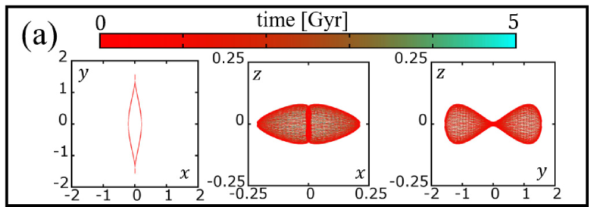
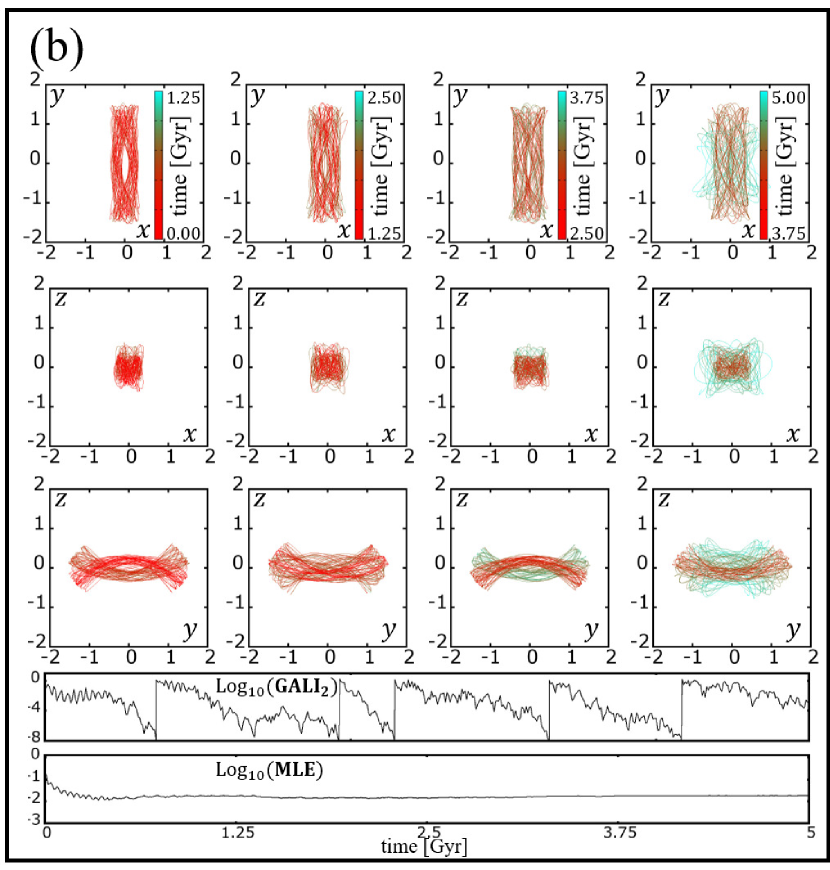
Figure 3: TI model A. (a) The $(x,y)$, $(x,z)$ and (y,z) projections (left, middle and right panel respectively) of a 3D regular orbit close to x1, integrated for 5 Gyr. (b) The evolution of an orbit close to x1v1 $(\Delta)$. In the upper three rows we see the evolution of the $(x,y)$, $(x,z)$, $(y,z)$ projections for times (left to right columns) $0\leq t\leq 1.25$ Gyr, $1.25<t\leq 2.5$ Gyr, $2.5<t\leq 3.75$ Gyr and $3.75<t\leq 5$ Gyr. The variation of its GALI₂ and MLE is shown at the bottom, elongated panels. (c) Similar to (b) but for an orbit close to x1v2 (U). The orbits are coloured according to their evolution in time, as indicated by the related colour bars.

The orbits described above represent in no case all kinds of non-periodic orbits one may encounter in the phase space of our system at the given E_J ​​. They are some of the orbits, which have been found in previous studies to shape the bar out of the equatorial plane. We will follow next the evolution of such orbits as the mass of the bar increases with time, in order to check if they retain or not their bar-supporting character. In this way we will compare the evolution of the same ICs in the TD case with those in TI models.

3.1.4 Successive autonomous models

A possible way of studying the evolution of a TD system is to rely on a sequence of potentials/models obtained from a sequence of snapshots from an $N$-body simulation (see e.g. the review by Athanassoula, 2013). Here we follow a similar route, i.e. we use a sequence of TI models, which we call the “shadow evolution” of the corresponding TD model. These TI models have successively increasing $M_{B}$ (or equivalently $GM_{B}$) between its minimum and maximum values. For example, in Fig. 4, we present the variation of the stability indices in a series of TI models, starting with the TI model A, in which $GM_{B}$ increases successively from 0.05 to 0.2, i.e. it quadruples. This series of TI models constitutes the shadow evolution of a TD model in which $M_{B}$ increases by the same amount within a predefined time interval.

The immediate information we obtain from the stability diagrams of Fig. 4, is whether or not a PO of a given family, at a certain E_J ​​, retains its stability as $GM_{B}$ varies. In addition, for any model in the range $0.05\leq GM_{B}\leq 0.2$, we can calculate the dynamics in the neighbourhood of any PO and compare it with the dynamics in the corresponding region of the TD model, when it reaches the same $GM_{B}$ during its evolution. Obviously, at the moment the orbit we evolve in the TD case reaches the $GM_{B}$ value we are interested in, it will have a different E_J than the one at the beginning of its integration. Thus, we want to compare its morphology with that of the orbit at the corresponding E_J of the autonomous model, as predicted by its location in the Poincaré surface of section at that energy. We will refer also to individual models in this series, as “shadow” models.

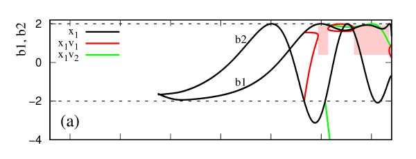
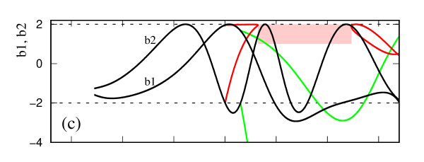
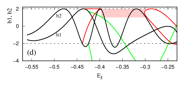
Figure 4: TI model A. Stability diagrams similar to the one of Fig. 1 for (a) $GM_{B}$=0.05, (b) $GM_{B}$=0.1, (c) $GM_{B}$=0.15 and (d) $GM_{B}$=0.2. The shaded pink areas indicate energy intervals where x1v1 is complex unstable. The successive TI models with increasing $GM_{B}$ constitute the shadow evolution of a TD model in which $GM_{B}$ increases by the same amount within a predefined time.

3.2 The non-autonomous case

In order to study the evolution of an orbit in a TD model, we start integrating an initial condition at the chosen initial energy. For model A, with $GM_{B}$=0.05, this is E_J =$-0.295$, because at this energy x1, x1v1 and x1v2 coexist. In all studied cases of the present work the quantity $GM_{B}$ increases linearly from the minimum to its maximum value.

In practice, it is not computationally feasible to examine the evolution of all orbits existing in a model as $GM_{B}$ increases. Moreover, we do not know a priori which orbits will be the important, bar-supporting ones in non-autonomous models. One can realize this by trying to navigate him/herself in a 4D space of section. For this reason, we selected characteristic cases of orbits, which have been already found to play an important role in supporting the thick part of rotating bars in autonomous models (Skokos et al., 2002a; Patsis et al., 2002; Patsis & Katsanikas, 2014a, b). We start from the main families of POs in the ILR region (x1, x1v1, x1v2) and we apply perturbations along directions chosen merely by our experience. In this effort, for model A, we have used as compass Figs. 2a,b. In particular, we investigate the following cases:

3.2.1 FAST $GM_{B}$ INCREASE

In the first TD model, the quantity $GM_{B}$ increases from 0.05 to 0.2, i.e. it quadruples within 5 Gyr. At the same time, $GM_{D}$ decreases so that the masses of the three components at each time step continue to satisfy the condition $G(M_{D}+M_{S}+M_{B})=1$. The initial energy in all examined cases for model A, is E_J =$-0.295$, as it was in the TI case, discussed in Section 3.1.

Evolution of ICs of POs in the TD model:

1. The evolution of x1: The first PO to be investigated is x1, on the equatorial plane of the galaxy. The x1 family is considered as the most important one in bar galaxy models. The x1 representative in Fig. 2 has ICs $(0.212...,0,0,0)$. Its morphological evolution is given in Fig. 5. In Fig. 5a we give it within the time interval 0-3.75 Gyr, while in Fig. 5b in the period $t$=3.75-5 Gyr. For this orbit, the corresponding GALI₂ index is presented in Fig. 5c. Remarkably, the shape of x1 persists for more than 3.75 Gyr (Fig. 5a and initial phase in Fig. 5b) and then it turns to a shape reminiscent of a bifurcation of x1 at the radial 3:1 resonance. As we know, the planar POs bifurcated at the radial 3:1 resonance are introduced in the system in pairs. The one with a morphology reminiscent of the one during the late stage evolution of the orbit in Fig. 5b has two representatives, symmetric with respect to the y-axis (see e.g. Skokos et al., 2002a). Thus, the presence of its both representatives in the $t$=3.75-5 Gyr time interval would support locally boxy isodensities. The evolution of the GALI₂ index (Fig. 5c) shows that the orbit we examine practically retains its regular nature during its 5 Gyr evolution despite its morphological change. We note, that GALI₂ does not register the orbit as chaotic when its morphological transformation occurs at $t\gtrapprox$3.75, since the orbit before and after that time remains regular. An indication of this transition between different regular behaviours, is the rather abrupt change of the inclination of GALI₂ at $t\approx$3.8. If for larger times, we consider the trace of the orbit on the Poincaré surfaces of section in the corresponding TI, i.e. in the shadow, models, we find that they are located on islands of stable 3:1 POs.

   

   Figure 5: Fast growing bar model A. Morphological evolution of x1 in the TD model (see text for details). In (a) during $t=$0-3.75 Gyr and in (b) during $t=$3.75-5 Gyr. The orbit is coloured according to time, as indicated by the colour bars to the right-hand sides of the panels. In (c) we give the time evolution of the GALI₂ index of the orbit.

2. The evolution of x1v1: We evolved the ICs $(0.212...,0.253...,0,0)$ of the x1v1 PO of the autonomous case, which for E_J =$-0.295$ is $\Delta$. Now, the exact shape of the orbit varies from the beginning of the integration. Nevertheless, as we can observe in Fig. 6, it retains some degree of regularity in its morphological evolution as it shows a clear bar-supporting character, both in its face-on and edge-on views, especially at the initial stages of its evolution. There is a gradual change of its relative dimensions by increasing its extent along the minor axis, something that becomes conspicuous in the last integration period ($3.75<t\leq 5$ Gyr) where the orbit is chaotic as the evolution of GALI₂ (Fig. 6d) indicates. Note that the orbit has an initial quasi-regular behaviour for $t\lessapprox 1.4$, as its GALI₂ did not reach the threshold $\log_{10}\mbox{GALI}_{2}\leq 10^{-8}$, which is followed by a chaotic epoch.

   

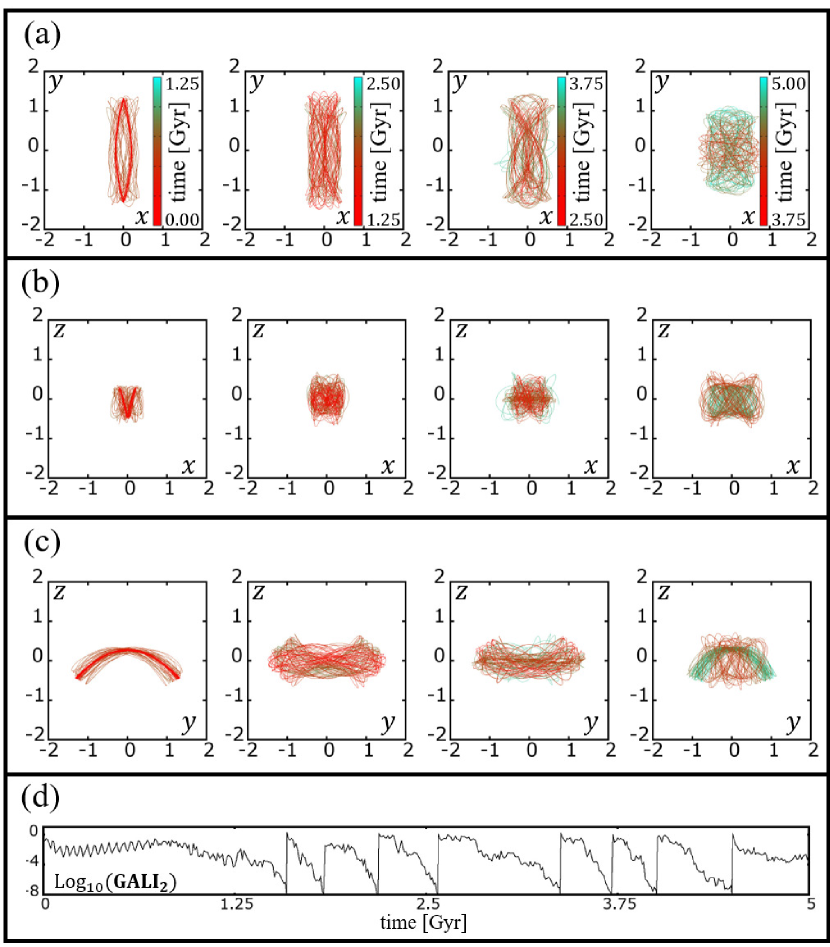
   Figure 6: Fast growing bar model A. The evolution, of the x1v1 PO in the TD system. Projections in the (x,y) (a), (x,z) (b), and (y,z) (c) planes, for times (left to right) $0\leq t\leq 1.25$ Gyr, $1.25<t\leq 2.5$ Gyr, $2.5<t\leq 3.75$ Gyr, $3.75<t\leq 5$ Gyr. The orbit in all projection panels is coloured according to time, as indicated by the colour bars in (a). (d) The time evolution of the GALI₂ index of the orbit.

   The orbital shapes we find in the projections of the orbits in Figs. 6a,b and c are typical of non-periodic orbits encountered in the ILR region of similar autonomous systems. The face-on projections (Fig. 6a) have initially a morphological transition from a x1-type shape to a shape encountered in face-on projections of orbits sticky to x1v1, supporting a face-on X feature (cf with figure 7 in Patsis & Katsanikas, 2014b) in the window $0\leq t\leq 1.25$ Gyr (first panel of Fig. 6a), lasting also for $1.25<t\leq 2.5$ Gyr (second panel). Then, during the next time interval, $2.5<t\leq 3.75$ Gyr (third panel), the morphology of the orbit is similar to that of the multiplicity 3 PO rm33 (see Table 4 in Patsis & Athanassoula, 2019). Finally, for $3.75<t\leq 5$ Gyr (fourth panel) we observe again the appearance of a face-on X feature, this time in a more squarish orbit. Here again we come across morphologies found in the autonomous models. In Patsis & Katsanikas (2014b) such orbits are found by relatively large perturbations in the $z$-direction (see figure 10d in that paper). In the first 3.75 Gyr the orbit supports a bar with similar length as the x1 PO in the region, while in the last time window, the orbit shrinks in the direction of the major axis of the bar, gaining width along the minor axis.

   The edge-on views of the orbit (Figs. 6b,c) reinforce a frown-smile morphology continuously during the 5 Gyr time interval. The prevailing side-on shapes are close to frowns (first and last panel in Fig. 6c), or smile-like (third panel), or hybrids (second panel), resembling the shapes of peanut-supporting orbits in the neighbourhood of $\Delta$ x1v1 POs presented in Patsis & Katsanikas (2014a).

   The morphological evolution and the variation of the GALI₂ index, resembles that of Fig. 3b, with the orbit being slightly more chaotic as more reinitializations of GALI₂ are observed in Fig. 6d, showing similar behaviours to chaotic orbits in the neighbourhood of x1v1 of the autonomous system. Actually, the orbit is always located in weakly chaotic zones around the x1v1 ICs of the corresponding “shadow”, autonomous models. The simultaneous boxiness in the face-on (Fig. 6a), edge-on (Fig. 6b) and side-on (Fig. 6c) projections is in agreement with the result of Patsis & Katsanikas (2014b) and Chaves-Velasquez et al. (2017) about the double boxiness of sticky chaotic orbits in rotating bars.

3. The evolution of x1v2: From the results we present in Fig. 7 it is evident that the U PO x1v2, with ICs $(0.210...,0,0,0.0591...)$ at E_J =$-0.295$ in the autonomous case, has in its face-on view a morphological evolution similar to x1 during the 5 Gyr integration period. Namely, its face-on view (Fig. 7a) presents the same transformation to a 3:1-like bifurcation of x1, as x1 does after 3.75 Gyr (Figs. 5a,b). The orbit in its side-on projection (Fig. 7b) is always restricted inside the known $\infty$-shape of the outline of the x1v2 POs in this projection. Notably, the height of the orbit is reduced with time and after 5 Gyr the resulting shape is almost planar. This evolution points to a regularly behaving orbit and this is confirmed by the evolution of the GALI₂ index (Fig. 7c).

   

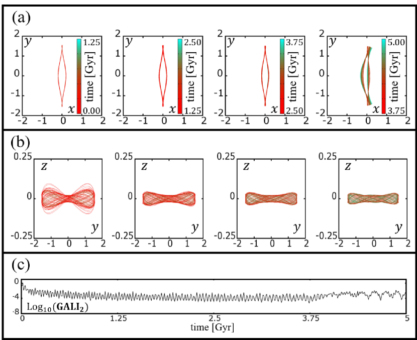
   Figure 7: Fast growing bar model A. The evolution, in the TD system, of the ICs of the x1v2 PO. The (x,y) (a) and (y,z) (b) projections for times (left to right) $0\leq t\leq 1.25$ Gyr, $1.25<t\leq 2.5$ Gyr, $2.5<t\leq 3.75$ Gyr, $3.75<t\leq 5$ Gyr. Note in (b) the different scale in the axes. The orbit in all projection panels is coloured according to time, as indicated by the colour bars in (a). (c) The time evolution of the GALI₂ index of the orbit.

   This result sounds counter-intuitive, since a U PO of the autonomous case behaves as regular when it evolves in the TD model. Nevertheless, this is not a property of these particular ICs, as also other x1v2 PO of the TI model we considered for different E_J values, show similar behaviours when they are evolved in the TD system. In order to understand this behaviour we checked the position of the evolved orbit in the phase space of the autonomous models of the shadow evolution taken at times in the middle of the four periods we plot our orbits throughout the paper (namely at $t=0.625$, 1.875, 3.125 and 4.375 Gyr, for which we respectively have $GM_{B}=0.06875$, 0.10625, 0.14374, 0.18125 and E_J =0.306, 0.328, 0.350, 0.372). In particular, we considered the locations of the $(x,z,p_{x},p_{z})$ coordinates of our orbit in the TD system by registering its upwards intersections with the $y=0$ plane for each time window. By placing these “traces” of the orbit on the $(x,p_{x})$ surfaces of section, as well as on the $(z,p_{z})$ projections of the shadow models, we realize that they correspond to points belonging to x1 tori. This is seen in Fig. 8 where these points are plotted with heavy red dots. It is clear that all red points in the first three time windows of Fig. 8a are very close to the initial conditions of x1 at the corresponding autonomous models. In the last period x1 appears unstable in the TI model (it is located between the two main stability islands on the $p_{x}=0$ axis) and the red points of the time-dependent orbit drift towards the stability islands of one of the bifurcated 3:1 orbits. The regular behavior of the orbit is also seen in its projections in the $(z,p_{z})$ plane (Fig. 8b) as its points always form a ‘ring’ distribution around the planar x1 orbit (denoted by the blue dot at $z=p_{z}=0$.) Thus, the morphological evolution of our orbit is fully in agreement with the dynamical behavior predicted by the models in the shadow evolution described in Fig. 4.

   

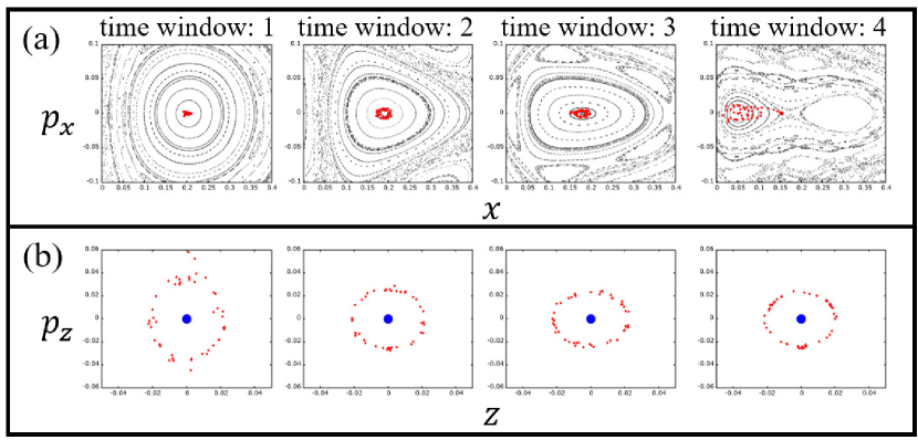
   Figure 8: Fast growing bar model A. (a) The $(x,p_{x})$ surfaces of section of the autonomous, “shadow” models at times (from left to right) $t=0.625$, 1.875, 3.125 and 4.375 Gyr (E_J and $GM_{B}$ values of the shadow models are given in the text). Heavy red dots indicate the “traces” of the orbit, starting with the ICs of the x1v2 PO of the TI model at E_J =$-0.295$, as it evolves in the TD system within each time window, 1: $0\leq t\leq 1.25$ Gyr, 2: $1.25<t\leq 2.5$ Gyr, 3: $2.5<t\leq 3.75$ Gyr, 4: $3.75<t\leq 5$ Gyr. (b) The $(z,p_{z})$ projection of the same orbit at the same time windows. The blue dot indicates the position of the x1 PO at $z=p_{z}=0$.

Evolution of ICs of non-POs of the TI model in the TD system:

Despite the fact that POs are the backbones of any barred model, the orbital content of real bars consists of non-POs (regular or chaotic). In studies of TI models, perturbations along certain directions have been proven particularly interesting for supporting observed structures, such as the peanut-shaped part of the bars. So, we examined the evolution of initial conditions along these directions in the TD model A:

1. Perturbations of x1: Firstly, we applied radial and vertical perturbations to the x1 representative of the autonomous model at E_J $=-0.295$. The radial x1 perturbations led in general to regular, bar-supporting, orbits with morphologies known from studies of TI models. Typical evolutions of perturbed x1 orbits are given in Fig. 9. In Figs. 9a,b the perturbed x1 orbits with ICs (0.212…,0,0.05,0) and (0.212,0,0.1,0) respectively, remain bar-supporting during the whole period of the 5 Gyr. However, especially in Fig. 9a, we observe a morphological transformation with time, associated with a weakly chaotic epoch during this transition, as the GALI₂ variation below the orbits indicates. Nevertheless, the orbit can always be characterized as bar-supporting. Similar morphologies are encountered when we start integrating in this TD model, initial conditions on the invariant curves in the neighbourhood of x1 of our TI model A (Fig. 2a).

   

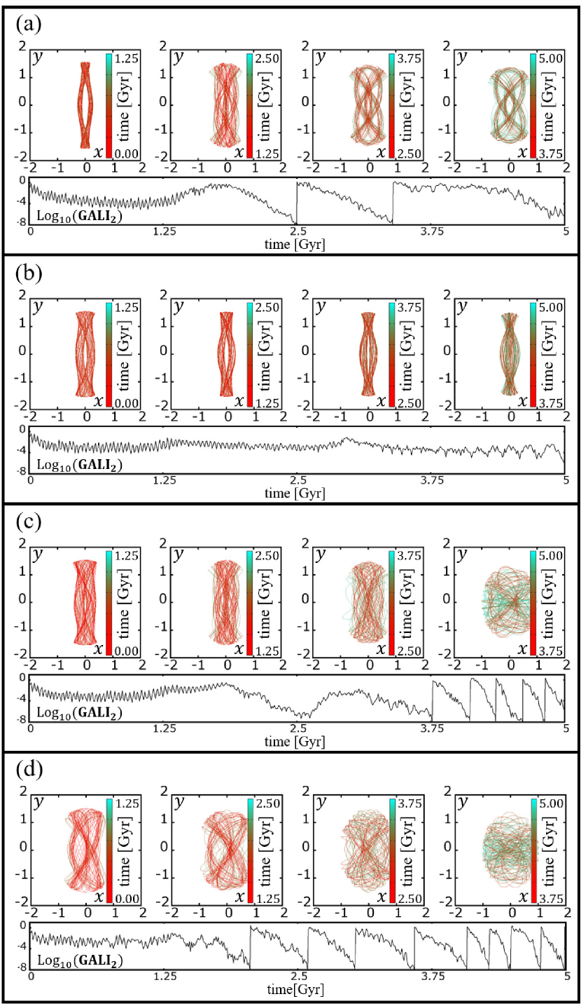
   Figure 9: Fast growing bar model A. The evolution of morphology and GALI₂ index of typical radially perturbed x1 orbits. The ICs of the orbits in (a) and (b) are on invariant tori around x1 in the autonomous case, while in (c) and (d) are located close to the edge of the x1 stability island, where chaos and tiny stability islands are present. Time windows and the colours of each orbit are as in Fig. 6.

   Morphologically, the evolution in Fig. 9a, leads from a x1- to a rm33-like (Patsis & Athanassoula, 2019) shape. The rm33 shape has been frequently encountered in the evolution of bar-supporting orbits in TD models in our study (see also figure 9 in Manos & Machado, 2014). Another frequently encountered evolution of perturbed x1 orbits is given in Fig. 9b. This is characterized by the prevalence of the ansae-type morphology as time increases. Effectively, this is similar to the transformation of the x1-like shape to a “double” 3:1 orbit (see also the discussion about boxiness due to 3:1 bifurcations of x1 in paragraph 3.2.1).

   Contrarily to the orbits in Figs. 9a,b, when we start integrating orbits located at the edge of the x1 stability island of the TI model, in a region dominated by the presence of tiny stability islands and chaotic zones (Fig. 2), we find only partly bar-supporting orbits. Two examples are given in Figs. 9c,d with ICs (0.212..,0,0.15,0) and (0.212..,0,0.2,0) respectively. Their GALI₂ variation, after an initial period of regular behaviour points to moderate chaoticity, especially during the last time windows. The orbit’s evolution for $2.5<t\leq 3.75$ Gyr in Figs. 9c is associated once again with the appearance of an X-feature in the face-on view of the orbit (Patsis & Katsanikas, 2014b; Tsigaridi & Patsis, 2015; Chaves-Velasquez et al., 2017). We also note that the orbit in Figs. 9d, supports during its regular phase in the first 2.5 Gyr an rm21-like (Patsis & Athanassoula, 2019) morphology.

   Small vertical x1 perturbations lead to ICs belonging to one of the invariant tori surrounding the PO in Fig. 2b. Qualitatively, their side-on projections remain morphologically invariant during the 5 Gyr period. In Fig. 10 we give the side-on profiles of an orbit, whose ICs are (0.212…,0,0, 0.05), during the first (a), and last (b), time windows. During the whole time of integration (5 Gyr), such orbits remain very close to the equatorial plane, thus for presenting their $\infty$-like shapes in this projection, the scales on the axes are not equal. We note though, that the height they reach is reduced as time increases, being minimum in the time interval 3.75-5 Gyr. In parallel, the face-on projections remain close to a x1 morphology up to $t=3.75$ and then we have again the usual in this model transformation to a 3:1-like morphology, similar to the one described in Figs. 5 and 7. We found similar evolution for all x1 orbits perturbed in the $p_{z}$ coordinate with $0.01\leq p_{z_{0}}\leq 0.6$. The GALI₂ variation is the characteristic one for regular orbits, so we avoid giving it here.

   

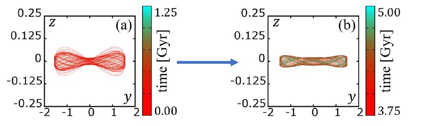
   Figure 10: Fast growing bar model A. The side-on view, in the TD system, of a perturbed by $p_{z}$ x1 orbit, starting on a torus surrounding the PO in the TI model. (a) The orbit during $0\leq t\leq 1.25$ Gyr and (b) during $3.75<t\leq 5$ Gyr. Note the different scales in the axes.

   At this point, before proceeding with investigating further the behaviour of non-POs in our TD potential, we would like to underline the following: Even if we increase the $p_{z}$ perturbation to reach the immediate neighbourhood of x1v2 in Fig. 2b the regular behaviour of the orbits in the TD potential persists. Starting with ICs (0.212…,0,0, 0.06) (cf. embedded frame in Fig. 2b) we observe again the regular behaviour seen in Fig. 10. This happens despite the fact that the orbit with the same ICs, (0.212…,0,0,0.06) in the TI potential has a chaotic behaviour during the 5 Gyr integration period. In Fig. 11 we give the evolution of the face-on (a), side-on (b) and the GALI₂ variation for this orbit. Evidently, it has a strong bar-supporting character only during the first 1.25 Gyr and consequently a totally different morphological evolution in its side-on profile compared with the orbit starting with the same ICs in the TD model (Fig. 10).

   

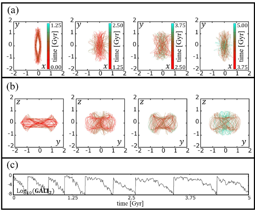
   Figure 11: TI model A. Plots similar to Fig. 7, but for an orbit with ICs (0.212…,0,0, 0.06), in the chaotic sea around x1v2. The same ICs integrated in the fast growing bar model A, give a regular orbit with morphologies similar to that of the orbits presented in Fig. 5 (face-on) and Fig. 10 (side-on).

   In a way we observe here a mechanism that organizes a chaotic orbit by adding time-dependency in the system. However, we can understand this behaviour by following the location of the orbit we integrate on the $(x,p_{x})$ and $(z,p_{z})$ projections of successive TI models in our shadow evolution. As $GM_{B}$ increases, the orbit moves closer to x1, in the stability region occupied by the invariant tori around x1 (Fig. 2b) and follows morphological patterns similar to those expected by integrating orbits on these x1 tori of the autonomous case. The traces of the orbit have a vary similar distribution on the surfaces of section of the autonomous models as those in Fig. 8.

   We move on now to the evolution of ICs of characteristic non-POs, in the neighbourhood of the two other main POs existing at this energy in the corresponding TI model.

2. Perturbed x1v1 orbits: In the autonomous model A, at E_J =$-0.295$, we have a x1v1 $\Delta$ representative. Thus, there are no quasiperiodic orbits around it. We have perturbed radially and vertically its initial conditions and have followed its evolution in the time-dependent case.

   Firstly, we examined the radial x1v1 perturbations. In all applied radial perturbations in the $x$-direction, i.e. for $0.25\leq x_{0}+\Delta x\leq 0.37$, where $x_{0}\approx 0.213$, all examined orbits were bar-supporting during the first 1.25 Gyr. For larger times, the supported bar structures were gradually dissolved. However, larger deviations from the $x_{0}$ coordinate of x1v1, do not necessarily lead to a faster drift into chaos. In Figs. 12a,b we respectively see the evolution of the face-on and side-on views of a characteristic orbit of this type, having ICs (0.37,0.253…,0,0). In this particular case, we have a deviation from the $x_{0}$ initial condition of x1v1 $|\Delta x_{0}|=0.157$ and the orbit is now partially bar-supporting for $t\lessapprox 2.5$ Gyr. The evolution of its GALI₂ index (Fig. 12c) indicates a chaotic character, which becomes more pronounced as soon as the morphology of the orbits ceases being bar-supporting.

   

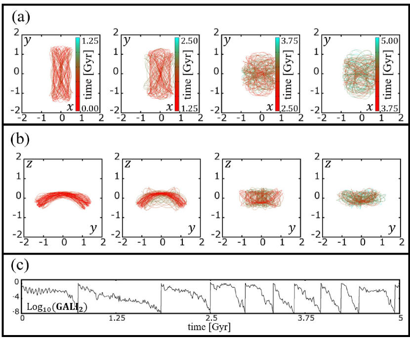
   Figure 12: Fast growing bar model A. Plots similar to Fig. 7 but for a characteristic bar-supporting orbit for $t\lessapprox 2.5$ Gyr, obtained as a radial perturbation of the x1v1 PO of the TI system.

   As regards vertically perturbed orbits in the neighbourhood of x1v1, most perturbations we applied in the $z$-direction, led to chaotic orbits. Nevertheless, in the neighbourhood of the PO $(0.18\leq z_{0}\leq 0.3,$ with $z_{0}$(x1v1) $\approx 0.253)$ the orbits are partially bar supporting, mainly during the first 1.25 Gyr.

3. Perturbed x1v2 orbits: By applying perturbations to the ICs of the U PO x1v2, we reach regions of phase space essentially already discussed in the presentation of the evolution of perturbed x1 orbits above. Radially perturbed x1v2 POs with $0.205<x_{0}<0.215$, led consistently to regular orbits similar to what we have presented in Fig. 10 with a frequent transition of the x1-like face-on shape to a 3:1-like one at times $t>3.5$ Gyr as in the case of Figs. 5 and 7. Vertical perturbations of the U x1v2 PO behave also in this case like regular orbits for long time intervals. This happens either because they are initially located on the x1 tori we observe in the $(z,p_{z})$ projection of the surface of section in the autonomous case (better seen in the enlarged frame in Fig. 2) and continue behaving as such in the TD evolution, or because there is a shifting of the traces of the orbits with respect to the surfaces of section of the corresponding autonomous models in the shadow evolution, as the one described in Fig. 8.

3.2.2 SLOW $GM_{B}$ INCREASE

Motivated by the growth of M_B in the $N$-body simulation by Manos & Machado (2014, see their Figure 2) we studied as well the evolution of characteristic orbits in models with a slow increase of the mass of the bar. There are long time intervals in $N$-body simulations, during which we have only a moderate or slow increase of M_B. Thus, starting with the same initial conditions of the orbits for E_J =$-0.295$, we studied the evolution of characteristic orbits when, during 5 Gyr, we have a growth of the mass of the bar from GM${}_{B}=0.05$ to GM${}_{B}=0.06$, i.e. when we have only a 20% increment.

Evolution of ICs of POs in the TD model:

1. The evolution of x1: The orbit with ICs the ones of the x1 PO of the TI model, remains practically unchanged during the 5 Gyr period (and for this reason we do not show it), as if it has been evolved in the TI model. It does not exhibit a transition to a 3:1-like morphology for $t>3.5$ Gyr, as in the previous, “fast” growing bar case (Fig. 5).

2. The evolution of x1v1: The evolution of x1v1 in the slow-growing bar model within 5 Gyr, can be described in general as similar to the one in the fast $GM_{B}$ growth case up to 3.75 Gyr (Fig. 6), and for this reason we do not plot it. We did not encounter the final shrinking of the orbit along the major axis in the late stage of its evolution, evident in the right panels in Fig. 6. Contrarily, despite being $\Delta$ in the autonomous case, when the bar is slowly growing, the orbit keeps practically its periodic orbital shape during the first time window ($t\leq 1.25$ Gyr). However, for larger times, it starts following a “thick-elliptical”, quasiperiodic-like morphology ($1.25<t\leq 2.5$ Gyr), and later it develops a weakly-chaotic ($2.5<t\leq 3.75$ Gyr) and eventually a chaotic character ($t>3.75$).

3. The evolution of x1v2: The orbit has a x1v2-like character with narrow $\infty$-type side-on profiles, as in the “fast” case (Fig. 3a) without even having the x1- to 3:1-like transition. The evolution of this orbit is again remarkable, given that its ICs correspond to a U PO in the autonomous model.

Evolution of ICs of non-POs of the TI model in the TD system:

The typical orbital dynamics in the TD system for orbits with ICs in the neighbourhood of the three main families of POs of the TI model can be summarized as follows:

1. Perturbations of x1: Radial perturbations of x1 lead to regular orbits with morphologies either similar to quasiperiodic orbits around x1, or with morphologies similar to POs of a higher multiplicity, existing at the x1 neighbourhood in the beginning of the integration. In the slowly growing bar model A, we do not find any further morphological evolution as in the radially perturbed x1 orbits of the “fast case” (Fig. 9). The orbits retain their initial shapes. Vertical perturbations of x1 in its immediate neighbourhood lead to the usual orbits with an envelope of $\infty$-like shape in their side-on views, for the cases with $0.01\leq p_{z}\leq 0.06$, we examined. Again here, the height of the orbits in the side-on projections is reduced with time.

2. Perturbations of x1v1: Firstly, we evolved orbits with ICs close to the $\Delta$ PO x1v1 of the autonomous case for E_J =$-0.295$, by varying its $x_{0}$ coordinate. As in the autonomous and in the fast growing bar case, smaller perturbations in the $x$-direction were not necessarily associated with more regular, or more bar-supporting orbits. The evolution of the orbits in this model is, in most cases, similar to the evolution of the orbits with the same ICs in the TI model. Thus, there are orbits which retain a frown or smile, quasiperiodic-like, side-on projection during the whole 5 Gyr period.

   Similar morphologies are encountered also in x1v1 orbits vertically perturbed along the $z$-direction. We find again ICs that seem to belong to a volume of phase space of the autonomous model, which, when evolved in the slowly bar growing model A, support the bar, however, this time for $t\lessapprox 2.5$ Gyr. To avoid redundancy we do not plot such orbits as they exhibit the same known patterns namely a quasiperiodic-x1-like face on view shape, combined with a “thick” frown, or smile, one in the side-on projections.

   Finally, an interesting class of morphological patterns encountered usually for $t\gtrapprox 2.5$ Gyr is presented in Fig. 13. The depicted, particular orbit has ICs (0.212…,0.18,0,0) and for $t\lessapprox 2.5$ Gyr retains a bar-supporting morphology with boxy face-on and a frown-smile side-on shapes. Nevertheless, we present it here for its morphology during the last part of its integration (two last panels of Figs. 13a,b,c). We also note that its GALI₂ indicator (Fig. 13d) points to a moderate chaotic orbit during the whole evolution. In the last two time windows of Fig. 13a its face-on views are round and its extents along the minor and major axes are almost equal (last panels in Fig. 13b and Fig. 13c for respectively the end-on- and the side-on views). Their overall size is comparable with that of the b/p part of the bar in our model. We want to underline at this point the appearance of a kind of X-shaped structure that can be observed in the edge-on views of orbits like this (both end-on and side-on). The sharpness of the X features and the angles of their wings make it rather unlikely to be combined with the X structures supported by orbits associated with x1v1 or x1v2 in a unique morphology.

   

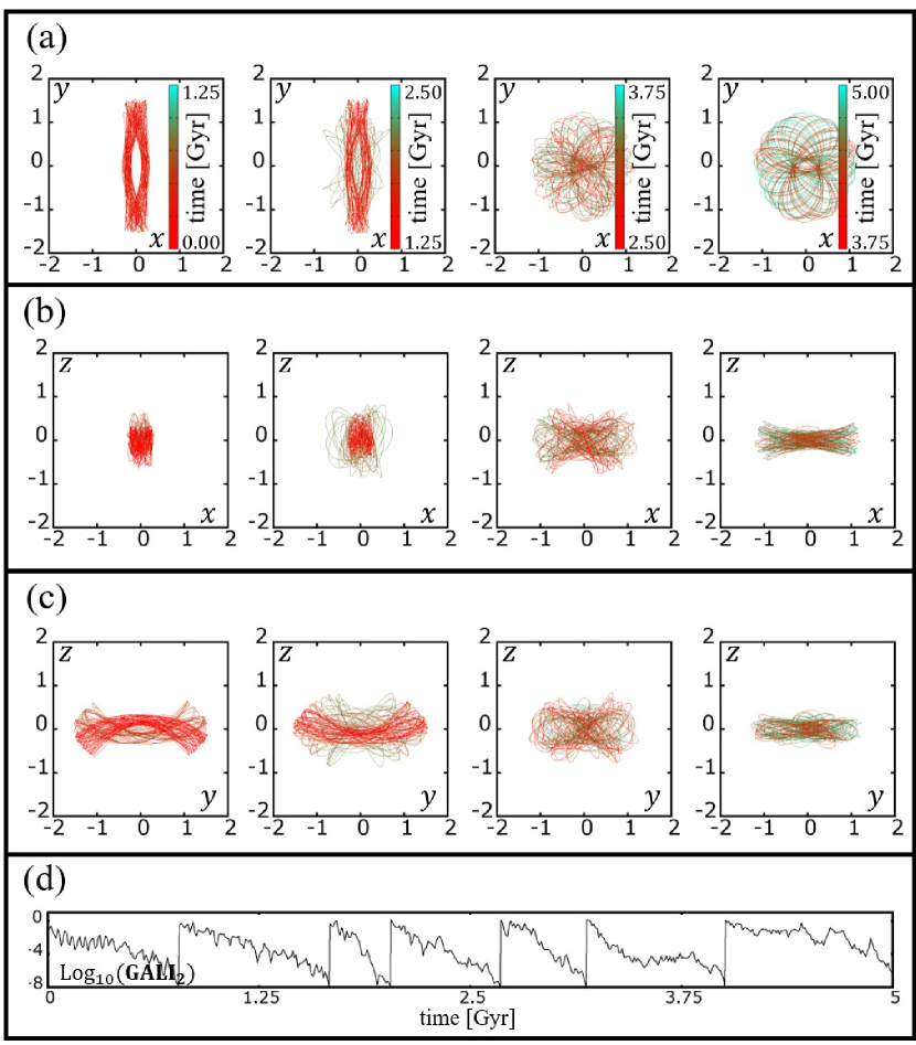
   Figure 13: Slowly growing bar model A. Plots similar to Fig. 7 but for a vertically perturbed x1v1 $\Delta$ orbit with a bar-supporting evolution for $t\lessapprox 2.5$ Gyr, which develops an X feature in the edge-on views for $t\gtrapprox 2.5$ Gyr, while the bar has been dissolved.

3. Perturbations of x1v2: Radially perturbed x1v2 orbits, in the immediate neighbourhood of the PO $(0.205\leq x_{0}(\rm{x1v2})\approx 0.21\leq 0.215)$, remain morphologically invariant as in all previous models we examined. They follow the usual shape with a x1v2-like envelope (Fig. 3a). The same holds for x1v2 orbits perturbed in the $p_{z}$-direction, with $|p_{z}|<|p_{z_{0}}\rm{(x1v2)}|$ as in the autonomous case (Fig. 2b). For $|p_{z}|>|p_{z_{0}}\rm{(x1v2)}|$ we find a zone with orbits that morphologically can be described as having hybrid x1v1-x1v2 morphologies, like e.g. the orbit with ICs (0.210…,0,0,0.63) (not shown in the paper). Despite the fact that in the autonomous model x1v1 is $\Delta$, this purturbed orbit behaves like a sticky one, trapped for a certain time around x1v1 tori of stable x1v1 POs (cf with figure 13 in Patsis & Katsanikas, 2014a).

4 Model B: A massive bar

Our model B is one with a massive bar already present at the beginning of its evolution, having $GM_{D}=$0.79, $GM_{S}$=0.08 and $GM_{B}$=0.13, which corresponds to a bar 2.6 times as massive as the bar of model A.

4.1 The autonomous case

Qualitatively, the evolution of the stability of the central family x1 is similar to the one in model A (comparable to the one in Fig. 4c). As energy varies, the two other main families, x1v1 and x1v2 are introduced in the system at the vILR of the model, at a standard S$\rightarrow$U$\rightarrow$S transition of x1. The x1v1 family is introduced as S, but soon after its bifurcation it becomes $\Delta$, changing back to S at a larger E_J ​​. The other 3D, 2:1 family, x1v2, is introduced as U and remains as such. We have chosen at the starting point the energy E_J = $-0.352$, in which x1v2, bifurcated from x1 at E_J =$-0.368$, has already b2$\approx-7.7$. Meanwhile x1v1 is complex unstable ($\Delta$) for E${}_{J}\gtrapprox-0.356$. The ICs of the main POs are for x1 (S) $(x_{0},z_{0},p_{x_{0}},p_{z_{0}})\approx(0.16,0,0,0)$, for x1v1 $(\Delta)$ about (0.152,0.277,0,0) and for x1v2 (U) about (0.142,0,0,0.223). The surfaces of section, which will help us in understanding the differences between the TI and TD cases for model B are depicted in Fig. 14.

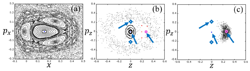
Figure 14: TI model B for E_J =$-0.352$. (a) The $(x,p_{x})$ surface of section around x1 (located at the center of the innermost stability island and indicated by a blue dot). (b) and (c) The $(z,p_{z})$ projection of the Poincaré section around x1 (blue point at $z=p_{z}=0$, which is also indicated by an arrow). The open circle symbol (accompanied by an arrow) indicates the location of x1v1, while the location of x1v2 ($p_{z}>0$) and x1v2^′ ($p_{z}<0$) are indicated with “diamonds” (with an arrow also showing the position of x1v2). Note in (b) the presence of the five tori (coloured in red) of a quasiperiodic orbit surrounding the $\Delta$ x1v1 PO. Black points in (b) correspond to vertical perturbations of x1, while in (c) they belong to several orbits with ICs in the neighbourhood of the x1v1 PO.

• Orbits in the x1 neighbourhood: The shape of the radially perturbed x1 orbits are the predicted by their location in the $(x,p_{x})$ surface of section (Fig. 14a). A significant difference with respect to model A, is that in model B, at E_J $=-0.352$, there are no rm21/rm22 orbits, as the absence of the characteristic four islands around x1 in Fig. 14a indicates. However, a major zone around the central x1 region is occupied by the stability islands of a 3-periodic orbit belonging to the rm33 family (Patsis & Athanassoula, 2019). Evidently, this affects the shape of the radially perturbed x1 orbits.

  Vertical perturbations of x1 (either in the $z-$ or $p_{z}-$direction) lead to x1v2-type morphologies, with $\infty$-like envelopes in their side-on projections, as in Fig. 3a. This happens as long as the ICs of the orbit are projected inside the area located in Fig. 14b between the ICs of x1v2 and x1v2^′ (diamond points), which is occupied by tori around x1. Beyond this region, we find weakly chaotic and chaotic orbits, determined by the structure of the phase space in the neighbourhood of the two other main families, x1v1 and x1v2 (see below).

• Orbits in the x1v1 neighbourhood: Perturbed x1v1 orbits, in the $x$-direction, in the interval $0.13\leq x_{0}\leq 0.22$ (with $x_{0}$(x1v1) = 0.1517…), have consistently a regular character, reflecting a quasiperiodic-like morphology that could be vaguely described as a “thick” x1v1 PO. For slightly larger perturbations, e.g. for $x_{0}$ = 0.25, we still have a frown side-on profile, combined with boxy, face-on projections that harbour an X feature, which is typical of sticky orbits (Patsis & Katsanikas, 2014a; Chaves-Velasquez et al., 2017).

  Similar is the orbital dynamics of the vertically perturbed x1v1 orbits in the $z$-direction, with $z_{0}<z_{0}$(x1v1)$\approx 0.276$. There is a clear tendency in the autonomous model B to support x1v1-like structures for larger perturbations and longer times than in model A, despite the fact that initially, in both cases, we have $\Delta$ x1v1 POs. A difference we traced between the two models is the presence of a 5-periodic orbit with tori close, around the initial conditions of x1v1. The projections of these tori in the $(z,p_{z})$ plane, for a quasiperiodic orbit with initial conditions (0.160…,0.2,0,0), are depicted with red colour in Fig. 14b. Although these 5 tori do not isolate the consequents of orbits in the neighbourhood of x1v1, they delay their diffusion to larger volumes in phase space, as can be seen in Fig. 14c from the accumulation of black points around the position of the x1v1 PO. Despite the fact that in 3D systems tori cannot isolate volumes of phase pace, such situations definitely increase the importance of $\Delta$ orbits, such as x1v1 in the specific case.

• Orbits in the x1v2 neighbourhood: Radial perturbations of the U PO x1v2, lead in general to weakly chaotic orbits. In a first approximation we can say that the closer to the ICs of the PO we start integrating an orbit, the longer it stays bar-supporting. However, we encounter also cases in which bar- and non-barred suporting phases alternate during the 5 Gyr period. The GALI₂ indicator of such orbits indicates in many cases a weakly chaotic character, while the orbits support of double boxiness with X features embedded in their face-on views.

  Vertical perturbations of x1v2 in the $p_{z}$-direction follow the behaviour we encountered in all models. Namely, for $|p_{z_{0}}|<|p_{z_{0}}\rm{(x1v2)}|$ the orbits are regular, with $\infty$-type envelopes in their side-on profiles, while for $|p_{z_{0}}|>|p_{z_{0}}\rm{(x1v2)}|$ they become gradually chaotic.

4.2 The non-autonomous case

4.2.1 FAST $GM_{B}$ INCREASE

Starting from the orbits existing in the autonomous case with $GM_{B}$=0.13, for E_J =$-0.352$, we follow first their morphological evolution when we have an increase of $GM_{B}$ from 0.13 to 0.52 within 5 Gyr. As for model A, also for model B, this means that the mass of the bar quadruples.

Evolution of ICs of POs in the TD model:

1. The evolution of x1: The evolution of the PO x1 in model B is towards the same shape as in the fast evolving model A (i.e. from a x1-like to a 3:1-like morphology, Fig. 5a), but faster. The 3:1-like shape is continuously present for $t\gtrapprox 1.5$ Gyr, instead of 3.75 Gyr in model A.

2. The evolution of x1v1: We find a remarkable persistence to a morphology typical for quasiperiodic orbits around x1v1 in the autonomous model, especially in the side-on projections, during the 5 Gyr period. The face-on view, for $t\lessapprox 1.5$ Gyr, is slightly asymmetric towards a quasiperiodic rm21 morphology. With increasing time this effect weakens, although existing, and eventually the orbit is elliptic-like for $t\gtrapprox 3.75$ Gyr. Comparing this evolution with our results in the low mass bar case of model A (Fig. 6), we observe that the role of x1v1 is pronounced in model B, in which initially the bar is 2.6 times more massive than in model A. This is associated with the structure of the phase space in model B, which is characterized by the presence of chains of stability islands around x1v1.

3. The evolution of x1v2: The evolution of x1v2, in its side-on view, is similar to that of x1v2 in model A, in the sense that it keeps the $\infty$-type morphology of its envelope during the 5 Gyr period, becoming narrower with time. The face-on view evolution is, like that of x1 in model B, from x1-like-quasiperiodic to 3:1-like-quasiperiodic (Figs. 5a,b). However, in model B, the 3:1 character is discernible already for $t\gtrapprox 1.5$ Gyr.

Evolution of ICs of non-POs of the TI model in the TD system:

1. Perturbations of x1: Radially perturbed x1 orbits evolve as x1 itself. Namely, there is a transition from the x1-like to the 3:1-like morphology, that occurs for times $t>1.5$ Gyr. Nevertheless, whenever the applied perturbation brings the initial conditions in the rm33 zone (the region of the three stability island around the innermost island of x1 in Fig. 14a), the orbit evolves keeping its rm33-like shape (as in the three right panels of Fig. 9a) during the whole period of the 5 Gyr, reducing its extent along the major axis of the bar with time.

   The evolution of perturbed in the vertical direction x1 orbits, depends, in general, on their ICs at the beginning of their evolution. A general description of orbits with $0.03\leq z_{0}\leq 0.15$ is that an initially ansae type face-on morphology, is changing to one that can be described as a “right parenthesis”. The larger the $z_{0}$ perturbations, the later the time the transformation occurs. The ansae shape is formed as the orbit librates between two parentheses-like structures, a left and a right one, symmetric with respect to major axis of the bar. Finally, the “right parenthesis”-like one prevails in the orbits we investigated. This can be seen in Fig. 15a, where we depict the face-on projections of the orbit with initial conditions (0.16,0.15,0,0) and initial E_J =$-0.352$. The parentheses patterns strongly resemble orbits belonging to the o1 family found in a strong bar model by Skokos et al. (2002b, their figure 17). However, the orbit we present here is 3D. The side-on projections, after an initial hybrid x1v1/x1v2-like morphology for $t\leq 1.25$ Gyr, develop the standard $\infty$-shaped outline (Fig. 15b) with the tendency to become planar with increasing time. This latter morphology dominates in the evolution of all vertically perturbed x1 orbits we discuss here, during the largest part of the 5 Gyr time period. The evolution of the GALI₂ index (Fig. 15c) is in agreement with the morphological evolution of the orbit, revealing the transition from an initially weakly chaotic behaviour to a more regular evolution at later times. For even larger $z_{0}$ values, we find boxy face-on projections combined with frown-smile, boxy, side-on views. For example, for $z_{0}=0.2$, the double boxy morphology follows an initial (t$\leq$ 1.5 Gyr) phase during which we find the imprint of the multiplicity 5 orbit to which belong the five islands in Fig. 14.

   

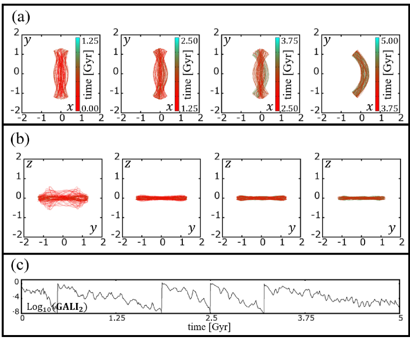
   Figure 15: Fast growing bar model B. Plots similar to Fig. 7 but for a vertically perturbed x1 orbit, which shows a typical morphological evolution in its face-on view from an ansae type to a parenthesis-like morphology (a), while in its side-on view the $\infty$-shaped outline dominates (b).

2. Perturbations of x1v1: Both radial and vertical perturbations of x1v1 lead to orbits that remain closer to x1v1-like morphologies for larger perturbation ranges than in model A. Radial perturbations in the range $0.13\leq x_{0}(\rm{x1v1})\approx 0.16\leq 0.22$ keep their frown side-on shapes, while their face-on projections can be briefly described as of distorted elliptical-like shapes. Deviations from the $z_{0}\approx 0.277$ IC keep their frown-like side-on morphologies during the 5 Gyr period, even if we reduce it to $z_{0}=0.18$, while for larger deviations from $z_{0}$ in this direction, these morphologies, resembling those of quasiperiodic orbits around x1v1, are transformed eventually to double boxy ones.

3. Perturbations of x1v2: The radially perturbed x1v2 orbits have a behaviour similar to the corresponding orbits in model A. The main difference is that in the face-on views now dominate the ansae-type shapes. In the side-on profiles we encounter again here the $\infty$-type envelopes of the orbits during most of the time of the 5 Gyr long integration interval. Their presence is associated with a more regular behaviour of the orbits. Whenever this side-on morphology is distorted, the GALI₂ index indicates a, weakly in general, chaotic character.

   Vertically perturbed x1v2 orbits of model B, lead, as in model A, either to the known orbits with the $\infty$-like morphologies in their side-on views, as long as the perturbation brings them on the tori of the 3D quasiperiodic orbits around x1, or to the hybrid x1v1/x1v2 side-on views, when they are away from this region. We note however, that in the latter case, frequently, weakly chaotic and regular phases alternate during the evolution of the orbits within 5 Gyr. This has as a result a rather constant support of the bar in the face-on view, combined however with different degrees of support of a bar component by different orbital shapes when viewed edge-on. We give an example in Fig. 16 of an orbit with ICs (0.141…,0,0,0.5). For $0\leq t\leq 1.25$ Gyr this orbit supports partly a bar. It has an irregular-boxy, face-on view (Fig. 16a) combined with a side-on profile harbouring an X feature. It reaches heights about 0.8 kpc away of the equatorial plane. In the time interval $1.25<t\leq 2.5$ Gyr the orbit has a more regular shape with a boxy face-on view and a clear smile-like, side-on one. Later, for $2.5<t\leq 3.75$ Gyr, the orbit behaves chaotically, returning to a morphology similar to its initial at the beginning of the integration, while for the last time interval ($3.75<t\leq 5$ Gyr) we have a narrow side-on prfile, combined with an asymmetric, bar-supporting, face-on projection. The GALI₂ index clearly captures all these changes in the orbit’s behaviour, as its several reinitializations in the time intervals $0\leq t\leq 1.25$ Gyr and $2.5<t\leq 3.75$ Gyr indicate the orbit’s chaotic nature, in contrast to its more regular evolution for $1.25<t\leq 2.5$ Gyr and $3.75<t\leq 5$ Gyr. where the reinitialization intervals became longer.

   

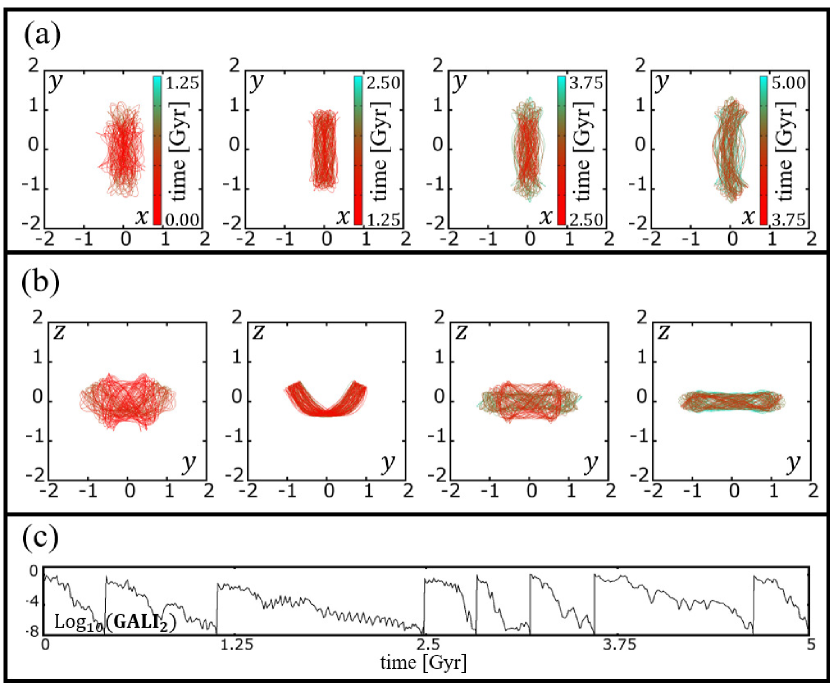
   Figure 16: Fast growing bar model B. Plots similar to Fig. 7 but for a vertically perturbed x1v2 orbit. The orbit is bar-supporting, but the supported bar morphologies, especially the side-on profiles vary.

4.2.2 SLOW $GM_{B}$ INCREASE

For the same model, B, we repeated our study considering that $GM_{B}$ increased within 5 Gyr from 0.13 to 0.156, i.e. by 20%. Again at the beginning of the integration the energy of the orbits we studied is E_J =$-0.352$.

Evolution of ICs of POs in the TD model:

1. The evolution of x1: In model B with $GM_{B}$ increasing slowly, as in the corresponding model A, the shape of x1 remains invariant during the integration period. There is no transition to 3:1-like shapes.

2. Also the shape of x1v1 remains quite invariant, despite being $\Delta$ at the starting point. This shape is characterized by a slightly triangular face-on view, while the two other projections are similar to those of quasiperiodic orbits around x1v1 in autonomous models (“thick” frowns or smiles).

3. The evolution of the x1v2 PO, which is U in the starting autonomous model, has also a regular character. The face-on projections resemble quasiperiodic orbits around x1, while the side-on views reinforce the morphology with the $\infty$-shaped outline. The same mechanism, which is being described in Fig. 8, is again in action. As a result, the evolution of an unstable orbit in a TD model, with slowly increasing bar mass in this case, leads to a regular behaviour.

Evolution of ICs of non-POs of the TI model in the TD system

1. Perturbations of x1: Radial perturbations of x1 evolve like quasiperiodic orbits in the autonomous case, reflecting the shapes of the POs, around which they are trapped, i.e. of x1 and rm33.

   The vertical perturbations of x1 evolve in a similar way like in the case of model B with the fast increase of $GM_{B}$. We find a large percentage of bar-supporting orbits with ansae-type face-on projections, where the orbit evidently follows the two parentheses-like shapes (cf. Fig. 15a), while the side-on views are either of $\infty$-type, or hybrid x1v1/x1v2-like. For perturbations beyond the $(z,p_{z})$ region occupied by the x1 tori (area between the two indicated with diamonds points in Fig. 14b), we find bar-supporting orbits with boxy face-on projections, typically for $t\lessapprox 2.5$ Gyr. For longer integration times, the orbits are only partly bar-supporting, or chaotic.

2. Perturbations of x1v1: Perturbations of the x1v1 ICs in the $x$-direction, in the range $0.13\leq x_{0}(\rm{x1v1})\approx 0.152\leq 0.22$, retain a sharp frown-like shape in their side-on views, while in their face-on projections we find patterns resembling quasiperiodic orbits trapped around, or being sticky, to x1 or to its higher multiplicity bifurcations (Patsis & Athanassoula, 2019). Frown-like shapes persist in a considerable range of perturbations in the $z$-direction.

3. Perturbations of x1v2: We find bar-supporting orbits by perturbing x1v2 orbits both radially and vertically. For perturbations in the $x$-direction, in the range $0.12\leq x_{0}(\rm{x1v1})\approx 0.142\leq 0.16$, the elliptical shapes in the face-on views, become boxy for $t\gtrapprox 3.75$ Gyr. In the side-on views prevail the frown- or smile-like patterns. This persistence of x1v1- or x1v1^′- shapes in the side-on projections is also encountered in the vertical perturbations of x1v2 in this model. Even orbits that start as weakly chaotic become later bar-supporting with frown- or smile-like side-on views. This is again related to the particular structure of phase space around the $\Delta$ x1v1 PO, which traps the orbits in a particular volume of it, as soon as the imposed perturbation brings its ICs in that phase space region.

5 Model C: A model without Complex Unstable x1v1 orbits

The next model in which we have investigated the evolution of orbits as $GM_{B}$ increases, is model C. In this model the individual mass components are $GM_{D}=0.878$, $GM_{S}=0.022$ and $GM_{B}=0.1$. The choice of these parameters leads to a model, in which the important x1v1 family has no $\Delta$ parts. The initial conditions of the main POs are for x1 (S) $(x_{0},z_{0},p_{x_{0}},p_{z_{0}})\approx(0.154,0,0,0)$, for x1v1 (S) about (0.15,0.144,0,0) and for x1v2 (U) about (0.149,0,0,0.076) at E_J =$-0.33$.

5.1 The autonomous case

The property of the x1v1 family, for which we have chosen the model, is demonstrated in the stability diagram given in Fig. 17. We observe that the stability indices of this family are always $-2<b1,2<2$, i.e. its POs are always S. We have chosen again an E_J to start with, at which all three main families of POs coexist. This is E_J =$-0.33$, for which x1 and x1v1 are S, while x1v2 is U. Guidelines for understanding the phase space structure at E_J =$-0.33$, can be taken again by plotting the $(x,p_{x})$ surface of section for the planar orbits (Fig. 18a) and the $(z,p_{z})$ projection of the 4D Poincaré cross section (Fig. 18b).

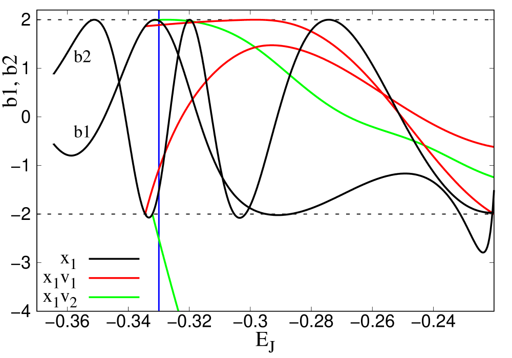
Figure 17: TI model C. Stability diagram similar to the one of Fig. 1. We observe that x1v1 is always S. The vertical blue line indicates the energy value E_J =-0.33.

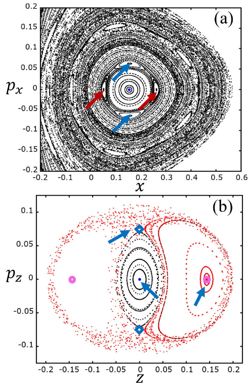
Figure 18: TI model C for E_J =$-0.33$. (a) The $(x,p_{x})$ surface of section around x1, located at the center of the innermost stability island (blue dot). Arrows point to the four islands of the multiplicity 2 POs, rm21 (red) and rm22 (blue) (b) The $(z,p_{z})$ projection of the Poincaré section around x1 (indicated by a blue dot and an arrow). Open circle symbols indicate the locations of x1v1 (right; also denoted by an arrow) and x1v1^′ (left), while the location of x1v2 ($p_{z}>0$; also denoted by an arrow) and x1v2^′ ($p_{z}<0$) are indicated with “diamond” symbols. Black points correspond to vertical perturbations of x1, while red points belong to several orbits with ICs in the neighbourhood of the x1v1 PO.

• Orbits in the x1 neighbourhood: As we can see in Fig. 18a, the $(x,p_{x})$ surface of section in the x1 region is characterized by islands of stability belonging to higher multiplicity bifurcations of x1. There is little chaos in the x1 neighbourhood. Consequently, by perturbing x1 radially, we displace the ICs of the orbit we want to study on some invariant curve around x1 or on an invariant curve belonging to a stability island of another family (e.g. on the four islands of rm21/rm22, denoted respectively by red/blue arrows). Practically, we always have a regular bar-supporting orbit, either by considering a single quasiperiodic orbit, or two, symmetric orbits, as e.g. in the case of rm21 and rm22.

  Also by applying vertical perturbations to x1, we reach tori of quasiperiodic orbits. By perturbing x1 in the $p_{z}$-direction, we find, as $|p_{z}|$ increases, for $|p_{z}|<|p_{z_{0}}(\rm{x1v2})|$ again the orbits with the expected $\infty$-shaped side-on profiles of the invariant-like curves around x1 in the central region of Fig. 18b. For larger $|p_{z}|$ perturbations, hybrid x1v1/x1v2-like side-on projections substitute the “$\infty$” shape profiles.

• Orbits in the x1v1 neighbourhood: In the absence of ($\Delta$) regions, radial and vertical perturbations of x1v1 orbits lead in the first place to quasiperiodic orbits around them, having the expected morphologies of such orbits encountered in autonomous models. Namely, we have frown-like quasiperiodic orbits around x1v1 and smile-like quasiperiodic orbits around x1v1^′. This is expected, since in model C we do not have any kind of a chaotic zone around x1v1 and x1v1^′, but invariant tori surrounding them in the 4D space of section, as those described in (Katsanikas & Patsis, 2011).

• Orbits in the x1v2 neighbourhood: Radial and vertical perturbations of x1v2 lead to morphologies that can be inferred by considering its initial conditions on the projections of the surfaces of section depicted in Fig. 18. The difference with respect to the previous studied cases, is that in the region surrounding x1v1 and x1v1^′ are occupied by tori on which perturbed x1v2 orbits may become sticky.

5.2 The non-autonomous case

5.2.1 FAST $GM_{B}$ INCREASE

Starting from the orbits existing in the autonomous case for E_J =$-0.33$, we follow first their morphological evolution when we have an increase of $GM_{B}$ from 0.1 to 0.4 within 5 Gyr. Like in the two previous models, this means that the mass of the bar quadruples.

Evolution of ICs of POs in the TD model:

1. The evolution of x1: The evolved x1 orbit remains practically invariant as in the autonomous case.

2. The evolution of x1v1: The x1v1 orbit keeps a x1v1-like morphology of a quasiperiodic orbit close to a periodic one. However, there is a clear tendency of the extent of the x1-like ellipse in the face on views to shrink with time. Namely, its projection on the major axis of the bar, the y-axis, becomes shorter.

3. The evolution of x1v2: The x1v2 orbit evolves similar to x1 orbits, perturbed in the $p_{z}$ direction. It has a quasiperiodic x1-like face-on and the known “$\infty$” side-on, overall shape. As in many previous cases we presented up to now, also in model C, the side-on profile becomes more narrow with time.

Evolution of ICs of non-POs of the TI model in the TD system:

1. Perturbations of x1: Radial perturbations of x1 have always morphologies similar to quasiperiodic orbits around the PO of the autonomous case. They are elliptical-like, if located close to the x1 and form boxy structures, if their ICs are further away (alone or in symmetric pairs).

   Orbits that are vertical perturbations of x1 have in general morphologies resembling in their side-on views either quasiperiodic orbits around x1v1/x1v1^′ (“thick”, frown- or smile-like morphologies), or 3D, quasiperiodic orbits around x1 with overall $\infty$-like shapes. Their morphology is determined by the location of their ICs on the Poincaré sections of the shadow models.

2. Perturbations of x1v1: Radially and vertically perturbed ICs of the x1v1 PO lead to orbits with x1v1-like shapes. Varying $x_{0}$ in the $0.13\leq x_{0}\leq 0.22$ range we found orbits with edge-on quasiperiodic-x1v1-like morphologies, while in their face-on views we find in most cases the elliptical-like quasiperiodic x1 patterns. During their evolution we also encounter quasiperiodic rm21/rm22 morphologies in some time intervals.

   Vertically perturbed x1v1 orbits have similar behaviours with the vertically perturbed x1 orbits. They keep qualitatively their initial quasiperiodic x1v1 morphology for 5 Gyr, shrinking however along the major axis of the bar with time. Transition to double boxy morphologies during the integration time is observed when we start with ICs in the borders of the regions occupied by x1 and x1v1 tori (Fig. 18b.)

3. Perturbations of x1v2: Starting integrating orbits in the neighbourhood of x1v2 we find in general regular orbits. In order to find the tendencies for the morphological evolution of perturbed x1v2 orbits in the TD model Fig. 18b is proven again a useful tool. Starting from x1v2 and moving in the $p_{z}$-direction towards x1, we find the orbits with elliptical-like face-on and $\infty$-like side-on profiles.

   Regular orbits are encountered in the TD model C even away from the region with the main families of POs. Such orbits are characterized by boxy edge-on profiles with a possible profile evolution in the face-on views, where we have transitions from elliptical-like to boxy patterns. A typical example of this behaviour, for an orbit with ICs (0.148…,0,0,0.2) is given in Fig. 19. The face-on transition takes place for $t>3.75$ (Fig. 19a). The time evolution of the GALI₂ index (Fig. 19c) clearly indicates the regular behavior of the orbit as GALI₂ remains always larger than the threshold value $10^{-8}$. There is a characteristic difference with respect to boxy profiles we found in the others models, namely that they are not densely filled, probably because of trapping around quasiperiodic orbits of high multiplicity.

   

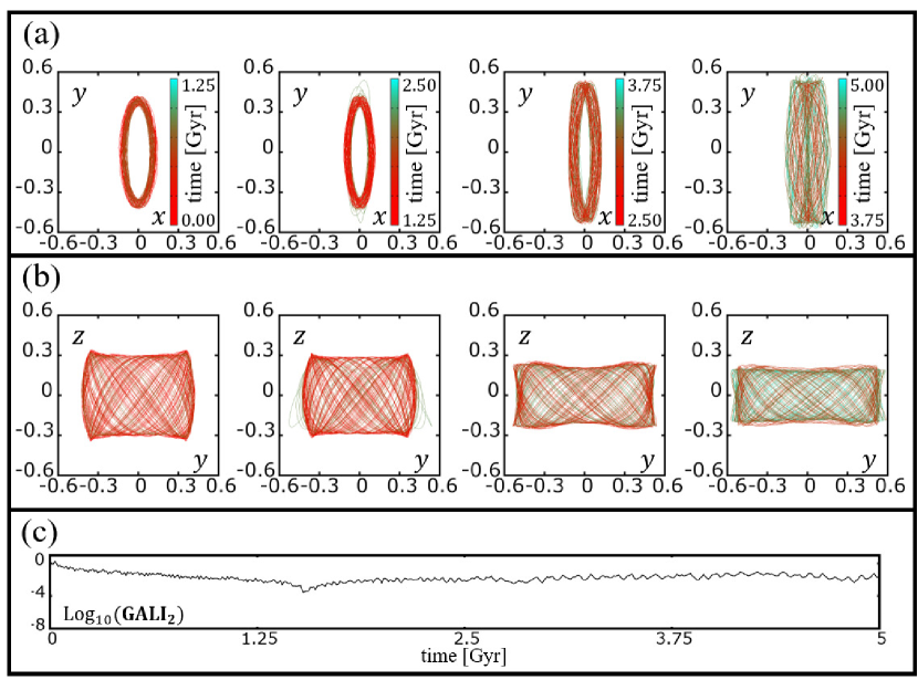
   Figure 19: Fast growing bar model C. Plots similar to Fig. 7 but for a vertically perturbed x1v2 orbit, with ICs displaced beyond the region of the neighbourhod of the three main families of the ILR region. The orbit has a regular character with boxy side-on profiles (see text).

5.2.2 SLOW $GM_{B}$ INCREASE

For model C, we repeated our previous study considering that $GM_{B}$ increases from 0.1 to 0.12, i.e. by 20%, within 5 Gyr. Also for the study of the slowly increasing $GM_{B}$ the considered orbits have initially E_J =$-0.33$.

Evolution of ICs of POs in the TD model:

The x1 and x1v1 orbits remain invariant during the 5 Gyr integration time. They retain their known morphologies as in the TI case. The orbit starting with the ICs of x1v2, has continuously a shape similar of an orbit on the invariant tori around x1 in the $(z,p_{z})$ projections of the surface of section. This is a morphology similar to the one in Fig. 3a, with elliptical, x1-like face-on projections, which remain as such during the whole integration period.

Evolution of ICs of non-POs of the TI model in the TD system:

1. Perturbations of x1: Perturbations of the x1 PO ($x_{0}(\rm{x1})\approx 0.154$) in the x-direction, lead to elliptical-like quasiperiodic orbits for $\Delta x_{0}\lessapprox 0.1$ and then become boxy. However, whenever the starting point is located in the vicinity of a regular PO of higher multiplicity, e.g. on one of the rm21/rm22 islands, a shape similar to that PO is preserved for the whole integrating period.

   Vertically perturbed x1 orbits remain in general regular in this model, with shapes similar to those of the vertically perturbed x1 orbits in the fast growing bar case of model C. Their evolution can be inferred by the morphology of the orbit at the starting point of the autonomous model, which remains practically invariant.

2. Perturbations of x1v1: All perturbations of x1v1 in the slowly growing bar model C, lead to regular orbits with quasiperiodic-like morphologies resembling quasiperiodic orbits around x1v1 in the autonomous case. Whenever a morphological evolution is observed, the traces of the orbit in the Poincaré sections of the corresponding autonomous models of the shadow evolution are found beyond the region occupied by the tori around x1v1 (or x1v1^′), as they appear in $(z,p_{z})$ projections similar to Fig. 18b. Such transitions are happening less frequently in the slowly increasing $GM_{B}$ model, because the deviations of the evolved orbits from the orbit of the TI model with the same ICs are small and the phase-space of the model is dominated by order.

3. Perturbations of x1v2: Radially perturbed x1v2 orbits, as long as their ICs are located beyond the central, lemon-shaped area, with the x1v2 and x1v2^′ POs at its peaks (Fig. 18b), have side-on views either with boxy morphologies, or with quasiperiodic-frown/smile-like shapes. The latter happens when the imposed perturbations bring them in the zone of influence of x1v1 (or x1v1^′). There are cases, for which we have a drift from an initial boxy morphology to a quasiperiodic-x1v1-like one, during the last phases of an orbital evolution. This reflects the gradual shift of the trace of the orbit in the shadow models, as $GM_{B}$ increases, to regions occupied by x1v1 tori. We note that the orbits, which evolve morphologically, show in general a delay in their evolution in the slowly growing bar case, compared with the fast growing one.

   Examining vertically perturbed x1v2 orbits ($p_{z}$(x1v2)$\approx 0.076$) in the $p_{z}$-direction, with $0.076\leq p_{z}\leq 0.2$, we always find boxy side-on profiles, similar to those of the perturbed x1v2 orbits of the fast growing bar case (Fig. 19b). During several time windows, these boxy shapes point clearly to side-on views of higher multiplicity periodic orbits as those presented in Patsis & Athanassoula (2019).

6 Summary and Conclusions

We have studied the evolution of specific orbits in Ferrers bars, in which the mass of the bar increases with time. We have examined two rates of bar growth within 5 Gyr. A fast one, in which the bar mass quadruples and a slow one, in which at the end of the integration the mass of the bar has increased just by 20%.

The orbits we investigated are those, which in TI models contribute mostly to the orbital content of the thick part of the bar, i.e. of the b/p bulge. This is the reason we concentrated ourselves in the study of the main orbital families, which provide the building blocks for thick bars. These are the families x1, x1v1 and x1v2, which start coexisting at the ILR region of the models. By using orbits associated with them, one can build profiles reproducing the observed edge-on morphology of boxy bulges, which are considered to be the part of the bar that extends well above the equatorial plane of the galaxy (see e.g. Athanassoula, 2005; Bureau et al., 2006; Athanassoula, 2016; Patsis et al., 2021).

Our goal is to find out the degree at which orbits starting with the same initial conditions as those in the autonomous case, continue to support a bar as the mass of the bar component of the potential increases. For this purpose it is important to know the regular or chaotic character of the orbits, although this fact does not secure by itself that they are bar-supporting or not. For determining the regular or chaotic nature of orbits during their time evolution we have used the GALI₂ index. In our study, we have also used (a) stability diagrams in the initial, autonomous models, which describe the evolution of the linear stability of the three main families of periodic orbits, (b) the $(x,p_{x})$ Poincaré sections, as well as appropriate projections in the $(z,p_{z})$ plane of the 4D cross sections of the autonomous case at the starting energy and (c) the shadow evolution of each model. This is a series of successive autonomous, “frozen”, models with the $GM_{B}$ values taken by the orbit we study during its integration.

The main conclusions of our study are:

1. The bar-supporting orbital morphologies found in TI models to support a b/p side-on profile, are encountered also in models, in which the mass of the bar increases with time. We did not find any orbital shapes not existing in autonomous models, which reinforce the peanut-shaped part of the bar.

2. The morphological evolution of the orbits observed in the TD models is gradual, even in the cases in which the mass of the bar quadruples within the integration time (5 Gyr). Contrarily to autonomous models, where we find variations in orbital morphologies only in the neighbourhood of unstable POs, the morphology of orbits in TD models may also vary in cases where an orbit remains practically regular during the integration time. In the majority of the studied cases, when a bar-supporting orbit ceases providing bar-supporting shapes, it becomes and remains chaotic for the rest of the time. Nevertheless, we also found cases, where bar-supporting and no-bar-supporting phases alternate (e.g. Fig. 16).

3. There is a good agreement between the morphology of an orbit in a time window and the location of its traces on the Poincaré cross section at the corresponding E_J in the autonomous model with the $GM_{B}$ value of the orbit at the time we are interested in. Thus, in a first approximation, we can understand the morphological evolution of an orbit in the TD potential as the series of morphological transformations expected by the displacements of its traces on the Poincaré sections during the shadow evolution. This applies especially to models with less chaos, as e.g. in the case of model C.

4. The role of the planar x1 orbits in the building of the 3D part of the bars has been emphasized in Patsis & Katsanikas (2014a, b) and in Chaves-Velasquez et al. (2017). The present study shows that this role can be even more important in TD models. The mechanism that leads to the reinforcement of the thick part of the bar, is based on the 3D morphology of the orbits on the tori around x1 in the 4D space of section and is in favor of “CX” (Bureau et al., 2006) side-on profiles. The orbits on these tori, with $x_{0}=x_{0}(\rm{x1})$, $|p_{z_{0}}|<|p_{z_{0}}(\rm{x1v2})|$ and $p_{x_{0}}=z=0$, are regular, with an $\infty$-type outline. However, in the autonomous models, if we have $|p_{z_{0}}|\geqq|p_{z_{0}}(\rm{x1v2})|$ we find initially sticky chaotic, and for larger $|p_{z_{0}}|$ chaotic, orbits. Such orbits, either offer a weaker support to the bar with hybrid x1v1/x1v2 side-on profiles, or no support at all. In the growing bar models we studied, with increasing time, an initial $|p_{z_{0}}|$ value with $|p_{z_{0}}|\gtrapprox|p_{z_{0}}(\rm{x1v2})|$, drifts towards smaller values and the orbit has a regular behaviour, evolving as belonging to quasiperiodic orbits in an autonomous model. A typical example is given in Fig. 8.

5. The regular or chaotic character of an orbit depends strongly on the structure of the phase space around it and in the way this phase space environment evolves during the time of integration. Thus, an initially quasiperiodic orbit, in a stability island surrounded by a chaotic sea, may evolve mainly as chaotic in the TD model. In parallel, an initially chaotic orbit, close to an unstable PO, in the TI model, may behave as regular, if there are stability islands of other orbits in its neighbourhood. The regular behaviour of orbits in the neighbourhood of simple unstable x1v2 orbits in all models with increasing in time $GM_{B}$ and partly the regular behaviour of orbits close to the complex unstable x1v1 orbit in model B, are due to the structure of the phase space around the POs.

6. Comparing the various studied models among themselves, we draw the following conclusions:

   (a) By evolving the same ICs, we find less morphological evolution in slowly than in fast growing $GM_{B}$ models.

   (b) We find more bar-supporting orbits in model B, in which we start with a more massive bar than in model A, in which the mass of the bar is at the beginning less massive. This is determined by the structure of phase space, especially around x1v1 (Fig. 14).

   (c) In model B with the massive bar, we found more planar orbits in the ILR region that support boxy shapes, than in the two other models. Vertical perturbations of such orbits retain boxy projections on the equatorial plane for a considerable range of the perturbations.

   (d) The ILR region of model C, with a marginal spheroidal component, is characterized by the dominance of large stability areas in phase space. This favours the persistence of structures like b/p bulges supported by regular orbits, as the mass of the bar increases with time.

In our time dependent models with the growing in time mass of the bar, time-dependency has contributed to the regularization of orbital motion, at least in the important for our study case of orbits in the vicinity of the initially unstable POs of the x1v2 family. This introduces a new way of supporting observed bar morphologies and particularly bars with “CX”-type side-on profiles. Future work should investigate whether this mechanism is in action in $N$-body models, especially during the growth phase of the bar.

Acknowledgements We thank Prof. G. Contopoulos for fruitful discussions and very useful comments. Ch.S. acknowledges support by the Research Committee (URC) of the University of Cape Town, and thanks the Research Center for Astronomy and Applied Mathematics of the Academy of Athens for its hospitality during his visits when parts of this work were carried out. This work has been been partially supported by the Research Committee of the Academy of Athens through the project 200/895.

Data availability The data underlying this article will be shared on reasonable request to the corresponding author.

References

- Athanassoula et al. (1983) Athanassoula E., Bienayme O., Martinet L., Pfenniger D. 1983, A&A, 127, 349
- Athanassoula (2003) Athanassoula E., 2003, MNRAS 341, 1179
- Athanassoula (2005) Athanassoula E., 2005, MNRAS 358, 1477
- Athanassoula (2013) Athanassoula E., 2013, in “Secular Evolution of Galaxies”, Falcon-Barroso J., and Knapen J.H. (eds.), Cambridge, UK: Cambridge University Press, 2013, p.305
- Athanassoula (2016) Athanassoula E., 2016, in ”Galactic Bulges”, E. Laurikainen, R. Peletier, D. Gadotti, (eds.), Springer International Publishing Switzerland, pp. 391-412
- Benettin et al. (1980a) Benettin G., Galgani L., Giorgilli A., Strelcyn J.-M., 1980a, Mecc, 15, 9
- Benettin et al. (1980b) Benettin G., Galgani L., Giorgilli A., Strelcyn J.-M., 1980b, Mecc, 15, 21
- Broucke (1969) Broucke R., 1969, NASA Techn. Rep., 32, 1360
- Bureau et al. (2006) Bureau M., Aronica G., Athanassoula E., Dettmar R.-J., Bosma A., Freeman K. C., 2006, MNRAS, 370, 753
- Chatzopoulos et al. (2011) Chatzopoulos S., Patsis P. A., Boily C.M., 2011, MNRAS, 416, 479
- Chaves-Velasquez et al. (2017) Chaves-Velasquez L., Patsis P. A., Puerari I., Skokos Ch., Manos T. 2017, ApJ, 850, 145
- Combes et al. (1990) Combes F, Debbasch F., Friedli, D, Pfenniger D., 1990, A&A, 233, 82
- Contopoulos (2004) Contopoulos G., 2004, “Order and Chaos in Dynamical Astronomy”, Springer-Verlag, Berlin, Heidelberg, New York
- Contopoulos & Grosbøl (1989) Contopoulos G., Grosbøl P., 1989, A&ARv, 1, 261
- Contopoulos & Harsoula (2008) Contopoulos G., Harsoula M., 2008, Int. J. Bifurc. Ch. 18, 2929
- Contopoulos & Magnenat (1985) Contopoulos G., Magnenat P., 1985, Celest. Mech. 37, 387
- Contopoulos & Papayannopoulos (1980) Contopoulos G., Papayannopoulos T., 1980, A&A, 92, 33
- Ferrers (1877) Ferrers, N. M. 1877, Quart.J.Pur.Appl.Math., 14, 1
- Hadjidemetriou (1975) Hadjidemetriou J., 1975, Celest. Mech., 12, 255
- Harsoula & Kalapotharakos (2009) Harsoula M., Kalapotharakos C., 2009, MNRAS, 394, 1605
- Katsanikas & Patsis (2011) Katsanikas M., Patsis P.A., 2011, Int. J. Bif. Ch., 21-02, 467
- Katsanikas et al. (2011) Katsanikas M., Patsis P.A., Contopoulos G., 2011, Int. J. Bif. Ch., 21, 2321
- Katsanikas et al. (2013) Katsanikas M., Patsis P.A., Contopoulos G., 2013, Int. J. Bif. Ch., 23-02, 1330005
- Lange et al. (2014) Lange S., Richter M., Onken F., Bäcker A., Ketzmerick R., 2014, Chaos, 24, 024409
- Machado & Athanassoula (2010) Machado R.E.G., Athanassoula E., 2010, MNRAS, 406, 2386
- Machado & Manos (2016) Machado R.E.G., Manos T., 2016, MNRAS, 458, 3578
- Manos & Machado (2014) Manos T., Machado R.E.G., 2014, MNRAS, 438, 2201
- Manos et al. (2012) Manos T., Skokos Ch., Antonopoulos Ch., 2012, Int. J. Bif. Ch., 22, 1250218
- Manos et al. (2013) Manos T., Bountis, T., Skokos, Ch., 2013, Journal of Physics A, 46, 25-4017
- Miyamoto & Nagai (1975) Miyamoto M., Nagai R., 1975, PASJ, 27, 533
- Moges et al. (2020) Moges H., Manos T., Skokos Ch., 2020, Nonlin. Phenom. Complex Syst., 23, 153
- Onken et al. (2016) Onken F., Lange S., Ketzmerick R., Bäcker A., 2016, Chaos, 26, 063124
- Patsis (2005) Patsis P.A., 2005, MNRAS, 358, 305
- Patsis et al. (1997) Patsis P. A., Athanassoula E., Quillen A. C., 1997, ApJ, 483, 731
- Patsis & Athanassoula (2019) Patsis P.A., Athanassoula E., 2019, MNRAS, 490, 2740
- Patsis & Harsoula (2018) Patsis P.A., Harsoula M., 2018, A&A, 612, 114
- Patsis & Katsanikas (2014a) Patsis P.A., Katsanikas M., 2014, MNRAS, 445, 3525
- Patsis & Katsanikas (2014b) Patsis P.A., Katsanikas M., 2014, MNRAS, 445, 3546
- Patsis et al. (2002) Patsis P.A., Skokos Ch., Athanassoula E., 2002, MNRAS, 337, 578
- Patsis et al. (2021) Patsis P.A., Xilouris E.M., Alikakos J., Athanassoula E., 2021, A&A, 647, 20
- Patsis & Zachilas (1994) Patsis P.A., Zachilas L., 1994, Int. J. Bif. Ch., 4, 1399
- Pfenniger (1984) Pfenniger D., 1984, A&A, 134, 373
- Plummer (1911) Plummer H.C., 1911, MNRAS, 71, 460
- Poincaré (1899) Poincaré H., 1899, Les Methodes Nouvelles de la Mechanique Celeste, Vol. III, Gauthier-Villars, Paris
- Richter et al. (2014) Richter M., Lange S., Bäcker A., Ketzmerick R., 2014, Phys. Rev. E, 89, 022902
- Skokos (2001) Skokos Ch., 2001, Physica D, 159, 155
- Skokos (2010) Skokos Ch., 2010, Lect. Notes Phys., 790, 63
- Skokos & Manos (2016) Skokos Ch., Manos T., 2016, Lect. Notes Phys., 915, 129
- Skokos et al. (2007) Skokos Ch., Bountis T.C., Antonopoulos Ch., 2007, Physica D, 231, 30
- Skokos et al. (2008) Skokos Ch., Bountis T.C., Antonopoulos Ch., 2008, Eur. Phys. J. Sp. Top., 165, 5
- Skokos et al. (2002a) Skokos Ch., Patsis P.A., Athanassoula E., 2002a, MNRAS, 333, 847
- Skokos et al. (2002b) Skokos Ch., Patsis P.A., Athanassoula E., 2002b, MNRAS, 333, 861
- Tsigaridi & Patsis (2015) Tsigaridi L., Patsis P.A., 2015, MNRAS, 448, 3081