Molecular properties from the explicitly connected expressions of the response functions within the coupled-cluster theory

Abstract

We review the methods based on expectation value coupled cluster formalism - a common framework for the derivation of properties: the ground-state average value of an observable, cumulants of the second-order reduced density matrices, polarization propagator, quadratic response function, and transition probabilities. We discuss the approximations and give examples of the most important numerical results.

1 Introduction

1.1 Molecular properties

The development of quantum chemical methods allows one to understand why physical phenomena occur and how to model them using computed physical properties of atoms and molecules: ionization energies, electron affinities, multipole moments, polarizabilities, intermolecular forces, and transition properties. In the past decades numerous ab initio quantum chemical methods were developed: the configuration interaction (CI)[1], Møller–Plesset perturbation theory (MP) also known as the many-body perturbation theory (MBPT), coupled cluster theory (CC),[2, 3] Monte Carlo methods,[4, 5, 6] and density-matrix renormalization group (DMRG)[7, 8, 9]. Those approximations can be employed as frameworks for the computation of the energy and properties of many-electron systems.

In general, molecular properties can be classified as energy difference properties, response properties, transition probabilities, internal interaction properties, internal structure properties and other kinds.[10] Consider a system with a time-dependent perturbation $V(t)$. One can expand the time-dependent expectation value of an observable $X$ in orders of the perturbation $V(t)$. The resulting terms are the time-independent expectation value of $X$, and linear, quadratic, cubic, and higher-order response functions. Since the work of Oddershede,[11, 12, 13] who introduced the concept of response functions into molecular physics, response theory has proven to be an important tool for the calculation of molecular properties.[14, 15, 13] This work focuses on the expectation value formalism of the coupled cluster theory (XCC) applied to response properties and transition probabilities.

1.2 Coupled cluster theory

The coupled cluster theory[16, 17, 2, 3] is the leading quantum-chemical wave function approach for describing of the electronic structure of small and medium-sized systems. The hierarchy of approximations in the CC theory provides an effective description of the electron correlation while retaining the size consistency.[18] The coupled cluster Ansatz is

$$\Psi=e^{T}\Phi,$$ (1)

where $\Phi$ is a reference determinant and $T$ is the coupled cluster excitation operator. Since the seminal works of Coester and Kümmel[16, 17] and later Čížek, [2] numerous applications of the method were reported[19] and general-purpose programs[20, 21] were developed. CC is routinely used for the computation of correlated ground-state energies, [22] molecular properties, [23, 24, 25] excited-state properties,[26] and analytical gradients.[27] It has been applied to atoms, molecules and extended systems.[28, 29, 30, 31]

The cluster operator $T$ for an $N$ electron system is a sum of single, double, and higher excitations, $T=T_{1}+T_{2}+\cdots+T_{N}$. The $n$-particle excitation operator $T_{n}$ is expressed as

$$T_{n}=\frac{1}{n!^{2}}\sum_{\mu_{n}}t_{\mu_{n}}\mu_{n},$$ (2)

where $t_{\mu_{n}}$ are the CC amplitudes, and $\mu_{n}$

$$\mu_{n}=e^{a_{1}a_{2}\ldots a_{n}}_{i_{1}i_{2}\ldots i_{n}}$$ (3)

denote the spin-orbital substitution operators $e^{p}_{q}$

$$\mu_{1}=e^{a_{1}}_{i_{1}}=a_{1}^{\dagger}i_{1}\qquad\mu_{2}=e^{a_{1}a_{2}}_{i_{1}i_{2}}=a_{1}^{\dagger}a_{2}^{\dagger}i_{2}i_{1}\qquad\ldots$$ (4)

$a_{1}^{\dagger}a_{2}^{\dagger}\ldots$ are creation operators and $i_{1}i_{2}\ldots$ are annihilation operators. The labels $a_{1},a_{2},\ldots i_{1},i_{2},\ldots p_{1},p_{2},\ldots$ are used for the virtual, occupied and general spinorbital indices. The ground-state energy is found by inserting Eq. (1) into the time-independent Schrödinger equation, multiplying from left by $e^{-T}$, and projecting onto the reference determinant. The amplitudes are obtained by projection onto excited determinants:

$$\langle\Phi|e^{-T}He^{T}|\Phi\rangle=E,$$ (5)

$$\langle\mu_{1}|e^{-T}He^{T}|\Phi\rangle=0,$$

$$\langle\mu_{2}|e^{-T}He^{T}|\Phi\rangle=0,$$

$$\ldots$$

$$\langle\mu_{N}|e^{-T}He^{T}|\Phi\rangle=0.$$

For many-electron systems, one needs to introduce approximations to keep the method computationally feasible. The natural choice is to truncate the $T$ operator at a given excitation level, obtaining CCD[2], CCSD[21, 32, 33], CCSDT,[34, 35, 36] etc. The next step is to neglect some terms in the amplitude equations as in the CC2[37] and CC3[38] approximations.

In the CCSD approximation, the operator $T$ is truncated after the double excitations, i.e., $T=T_{1}+T_{2}$. The computational cost of the ground-state energy and amplitudes scales as $N^{6}$, where $N$ is the size (number of electrons) of the system. In the CC2[37] method, the single amplitudes are computed in the same way as in CCSD. The double amplitudes are correct only through the first-order in the fluctuation potential $W$

$$W=H-F,$$ (6)

where $H$ is the Hamiltonian and $F$ is the Fock operator. The CC2 approximation scales as $N^{5}$.

For the full inclusion of the triple amplitudes, the CCSDT model[34, 35, 36] has to be used. However, the computational cost, $N^{8}$, limits its applications. Various approaches for approximate inclusion of the triple excitations are available in the literature, including CCSDT-1,[39, 40, 41] CCSD(T),[42] CC3[38] and SVD-CCSDT.[43] In the CCSD(T) model, it is unnecessary to explicitly solve for $T_{3}$ and the triple excitations are included only in the energy expression as the fourth- and fifth-order perturbation energy contributions. However this method is not suitable for the computation for the transition properties because of the perturbative inclusion of triples. By contrast, in the CC3 method, $T_{1}$ and $T_{2}$ are iterated in the presence of approximate $T_{3}$. The computational cost of obtaining $T_{3}$ in this method is $N^{7}$. The availability of iterative amplitudes makes CC3 a viable approach beyond-CCSD approach for the calculation of molecular properties. In the SVD-CCSDT method the scaling is reduced to $N^{6}$ from the original $N^{8}$ scaling of CCSDT by the use of tensor decomposition. This method has been published only recently and is a promising approximation to be applied together with the XCC method.

1.3 Response functions

A system with a time-dependent perturbation $V(t)$ is described by the Hamiltonian

$$H(t)=H_{0}+V(t),$$ (7)

where $H_{0}$ is the Hamiltonian of the unperturbed system and the perturbation can be written in a general, Hermitian form as a sum of periodic contributions[44]

$$V(t)=\sum_{k=-M}^{M}e^{-i\omega_{k}t}\sum_{y}\epsilon_{y}(\omega_{k})y$$ (8)

$\omega_{k}$ is the frequency of the perturbation and $\epsilon_{y}(\omega_{k})$ is the perturbation strength parameter. The following equalities hold for thus defined, Hermitian $V(t)$:

$$y^{\dagger} =y$$ (9)

$$\omega_{-k} =-\omega_{k}$$ (10)

$$\epsilon_{y}^{*}(\omega_{k}) =\epsilon_{y}(-\omega_{k}).$$ (11)

The expectation value of an observable $X$ is

$$\bar{X}(t)=\braket{\Psi_{0}(t)}{X}{\Psi_{0}(t)}.$$ (12)

Formally $\bar{X}(t)$ is obtained by solving the time-dependent Schrödinger equation

$$H(t)\Psi_{0}(t)=i\frac{\partial}{\partial t}\Psi_{0}(t),$$ (13)

and expanding the expectation value in orders of the perturbation

$$\bar{X}(t)=\bar{X}+\sum_{k}e^{-i\omega_{k}t}\sum_{y}\epsilon_{y}(\omega_{k})\braket{\braket{X;Y}}_{\omega_{k}}+\\ \frac{1}{2}\sum_{k_{1},k_{2}}e^{-i(\omega_{k_{1}}+\omega_{k_{2}})t}\sum_{y,z}\epsilon_{y}(\omega_{k_{1}})\epsilon_{z}(\omega_{k_{2}})\braket{\braket{X;Y,Z}}_{\omega_{k_{1}},\omega_{k_{2}}}+\ldots$$ (14)

The first term in this expansion, $\bar{X}$, is the time-independent expectation value. The coefficients $\braket{\braket{X;Y}}_{\omega_{k}}$, $\braket{\braket{X;Y,Z}}_{\omega_{k_{1}},\omega_{k_{2}}}$, etc. are the linear, quadratic and higher response functions, respectively, which describe the response of an observable $X$ to the perturbation $V(t)$.

There exist two approaches to the coupled cluster response theory. The first approach based on the differentiation of the CC energy expression was introduced by Monkhorst in 1977[45, 46] and later extended by Bartlett et. al,[47, 48, 49, 50] and is known as the $\Lambda$ operator technique. Koch and Jørgensen[51, 52, 53] proposed the time-averaged quasi-energy Lagrangian technique, which is referred to in this work as the time-dependent coupled cluster approach (TD-CC). That method requires the solution for the Lagrange multipliers in addition to coupled cluster amplitudes. Within that approach, its authors developed expressions for the linear, quadratic, and cubic response functions,[44] transition moments,[54] spin-orbit coupling matrix elements,[55, 56] and other properties,[57] at the CC2,[37, 58] CCSD,[59] and CC3 levels of theory.[38, 60]

The second approach is based on the computation of molecular properties directly from the average value of the operator $X$ using the auxiliary excitation operator $S$. To avoid confusion it should be noted that the XCC method considered in this work is different from the approach of Bartlett and Noga[61] bearing the same name. An extensive review of the $S$ operator method was published by Arponen and co-workers in the context of the extended coupled cluster theory (ECC).[62, 63, 64] The operator $S$ is defined in that work by a set of nonlinear equations to which no systematic scheme of approximations had been found. Later Jeziorski and Moszynski[65] investigated this problem and proposed an expression for $S$ that satisfies a set of linear equations and can be systematically approximated. Within this approach the average value of $X$ can be expressed through a finite series of commutators. As commutators cotain only contracted terms, the expression for the expectation value of $X$ is fully connected. This method was then extended by Moszynski et al. [66] to the computation of the polarization propagator.

To date, the XCC method[65] has been employed to compute various electronic properties: electrostatic[67] and exchange[68] contributions to the interaction energies of closed-shell systems, first-order molecular properties,[25] frequency-dependent density susceptibilities,[69] static and dynamic dipole polarizabilities, [24] and transition moments between excited states.[70, 71] A prominent application of the XCC formalism is the computation of symmetry-adapted perturbation theory (SAPT) contributions described in a series of publications by Korona et al.[72, 73, 69, 74]

2 Explicitly connected expansion of an observable’s average value

The expectation value in the coupled cluster theory is defined as

$$\bar{X}=\frac{\braket{\Psi}{X\Psi}}{\braket{\Psi}{\Psi}}=\frac{\braket{e^{T^{\dagger}}Xe^{T}}}{\braket{e^{T^{\dagger}}e^{T}}},$$ (15)

where we use a shorthand notation which skips the Hartree-Fock determinant:

$$\braket{X}\equiv\braket{\Phi}{X\Phi}$$ (16)

$$\ket{Xe^{T}}\equiv\ket{Xe^{T}\Phi}$$ (17)

and

$$\braket{X}{Y}\equiv\braket{X\Phi}{Y\Phi}.$$ (18)

The expansion of Eq. (15) in $T$ is infinite due to the presence of the $e^{T^{\dagger}}$ operator. However it can be reformulated with the use of an auxiliary operator $S$[62, 65]

$$e^{S}\Phi=\frac{e^{T^{\dagger}}e^{T}\Phi}{\braket{e^{T^{\dagger}}e^{T}}}.$$ (19)

as

$$\bar{X}=\frac{\braket{e^{T^{\dagger}}e^{T}}{e^{-T}Xe^{T}}}{\braket{e^{T^{\dagger}}e^{T}}}=\braket{e^{S}}{e^{-T}Xe^{T}}=\braket{e^{S^{\dagger}}e^{-T}Xe^{T}e^{-S^{\dagger}}}.$$ (20)

In the last equality we used identity b from Table 1.

Table 1: Identities used in the XCC derivations.

a)	$e^{-T}He^{T}=H+[H,T]+\frac{1}{2!}[[H,T],T]+\ldots$
b)	$\ket{e^{-S^{\dagger}}\Phi}=\Phi$
c)	$X\Phi=\braket{X}\Phi+\hat{\mathscr{P}}(X)\Phi$
d)	$1=e^{-T}e^{S^{\dagger}}e^{-S^{\dagger}}e^{T}$

The auxiliary operator $S$

$$S=S_{1}+S_{2}+S_{3}+\ldots$$ (21)

is an excitation operator and satisfies a linear equation, where $S_{n}$ is expanded in a finite commutators series[65]

$$S_{n} =T_{n}-\frac{1}{n}\hat{\mathscr{P}}_{n}\left(\sum_{k=1}\frac{1}{k!}[\widetilde{T}^{\dagger},T]_{k}\right)$$ (22)

$$-\frac{1}{n}\hat{\mathscr{P}}_{n}\left(\sum_{k=1}\sum_{m=0}\frac{1}{k!}\frac{1}{m!}[[\widetilde{S},T^{\dagger}]_{k},T]_{m}\right),$$

where

$$\widetilde{T}=\sum_{n=1}^{N}nT_{n}\qquad\widetilde{S}=\sum_{n=1}^{N}nS_{n}.$$ (23)

$[A,B]_{k}$ is a shorthand for a $k$-times nested commutator. The superoperator $\hat{\mathscr{P}}_{n}(X)$ yields the excitation part of $X$

$$\hat{\mathscr{P}}_{n}(X)=\frac{1}{n!^{2}}\sum_{\mu_{n}}\braket{\mu_{n}}{X}\mu_{n}.$$ (24)

The operator $S$ is explicitly connected.[65] Using the commutator expansion of $e^{-T}Xe^{T}$ the expectation value takes the form

$$\bar{X}=\braket{e^{S^{\dagger}}e^{-T}Xe^{T}e^{-S^{\dagger}}}=\sum_{k=0}\sum_{m=0}\frac{1}{k!}\frac{(-1)^{m}}{m!}\braket{\left[\left[X,T\right]_{k},S^{\dagger}\right]_{m}}.$$ (25)

Because $\bar{X}$ is expressed solely by the commutators of connected operators, it is explicitly connected. We assume that $X$ is a one-electron Hermitian operator. An arbitrary non-Hermitian operator can be represented as a linear combination of $X+X^{\dagger}$ and $i(X-X^{\dagger})$, which are both Hermitian.

Although the expression for $S_{n}$ is finite, it includes complicated terms with high powers of $T$, even when $T$ is truncated and therefore needs to be approximated. The expectation value $\bar{X}$ from Eq. (25) is also approximated independently of $S$. For example at the CCSD level the average value $\bar{X}$ becomes[25]

$$\begin{split}\bar{X}&=\braket{X}\\ &+\braket{S_{1}}{X}+\braket{XT_{1}}+\braket{S_{2}}{[X,T_{2}]}\\ &+\braket{S_{1}}{[X,T_{2}]}\\ &+\braket{S_{1}}{[X,T_{1}]}+\braket{S_{2}}{[[X,T_{1}],T_{2}]}\\ &+\frac{1}{2}\braket{S_{1}^{2}}{[X,T_{2}]}+\frac{1}{2}\braket{S_{1}S_{2}}{[[X,T_{2}],T_{2}]}\\ &+\frac{1}{2}\braket{S_{1}}{[[X,T_{1}],T_{1}]}+\frac{1}{2}\braket{S_{3}}{[[X,T_{2}],T_{2}]}\\ &+\frac{1}{2}\braket{S_{1}^{2}}{[[X,T_{1}],T_{2}]}\\ &+\frac{1}{12}\braket{S_{1}^{3}}{[[X,T_{2}],T_{2}]}.\end{split}$$ (26)

In general the approximations of Eq. (25) are guided by either MBPT expansion or expansion in powers of $T$.

2.1 MBPT expansion

The $T$ amplitudes can be expanded in orders of $W$[75]

$$T=T^{(1)}+T^{(2)}+T^{(3)}+\ldots$$ (27)

The amplitudes $T^{(n)}$, where $n$ is the MBPT order, are obtained with the resolvent

$$\mathscr{\hat{R}}_{n}(W)=\frac{1}{(n!)^{2}}\sum_{a_{n}i_{n}}\frac{\braket{e^{i_{1}\ldots i_{n}}_{a_{1}\ldots a_{n}}W}e_{i_{1}\ldots i_{n}}^{a_{1}\ldots a_{n}}}{(\epsilon_{i_{1}}+\ldots+\epsilon_{i_{n}}-\epsilon_{a_{1}}-\ldots-\epsilon_{a_{n}})}$$ (28)

$$T^{(1)}=T_{2}^{(1)}=\hat{\mathscr{R}}_{{2}}(W)$$ (29)

$$T_{n}^{(2)}=\hat{\mathscr{R}}_{{n}}([W,T_{2}^{(1)}]),\qquad n=1,2,3$$ (30)

$$T_{1}^{(3)}=\hat{\mathscr{R}}_{{1}}([[W,T_{1}^{(2)}+T_{2}^{(2)}+T_{3}^{(2)}]).$$ (31)

The corresponding MBPT approximations to $S$ are

$$S^{(1)}=T^{(1)}$$ (32)

$$S^{(2)}=T^{(2)}$$ (33)

$$S_{1}^{(3)}=T_{1}^{(3)}+\hat{\mathscr{P}}_{1}\left([T_{1}^{(2)\dagger},T_{2}^{(1)}]\right)\\ +\hat{\mathscr{P}}_{1}\left([T_{2}^{(1)\dagger},T_{3}^{(2)}]\right)$$ (34)

$$S_{2}^{(3)}=T_{2}^{(3)}+\frac{1}{2}\hat{\mathscr{P}}_{2}\left([[T_{2}^{(1)\dagger},T_{2}^{(1)}],T_{2}^{(1)}]\right).$$ (35)

To obtain $\bar{X}$ at a given MBPT order, one takes only selected terms from Eq. (25)

$$\bar{X}^{(0)}=\braket{X}$$ (36)

$$\bar{X}^{(1)}=0$$ (37)

$$\bar{X}^{(2)}=\braket{S_{1}^{(2)}}{X}+\braket{XT_{1}^{(2)}}+\braket{S_{2}^{(1)}}{[X,T_{2}^{(1)}]}$$ (38)

$$\bar{X}^{(3)}=\braket{S_{1}^{(3)}}{X}+\braket{XT_{1}^{(3)}}+\braket{(T_{1}^{(2)}+T_{2}^{(2)}+T_{3}^{(2)})}{[X,T_{2}^{(1)}]}+\\ \braket{T_{2}^{(1)}}{[X,(T_{1}^{(2)}+T_{2}^{(2)}+T_{3}^{(2)})]}.$$ (39)

2.2 Expansion in powers of $T$

In practice, it is easier to apply an expansion in powers of $T$. The $T$ amplitudes are first computed from the conventional CC theory. The $S$ amplitudes in this approach are expanded in powers of $T$, giving the following equations in the CCSD case

$$S^{[1]}_{n}=T_{n}$$ (40)

$$S_{1}^{[2]}=\hat{\mathscr{P}}_{1}\left([T_{1}^{\dagger},T_{2}]\right)$$ (41)

$$S_{2}^{[3]}=\hat{\mathscr{P}}_{2}\left(\frac{1}{2}[[T_{2}^{\dagger},T_{2}],T_{2}]+[[T_{1}^{\dagger},T_{2}],T_{1}]\right)$$ (42)

$$S_{1}^{[3]}=\hat{\mathscr{P}}_{1}\left(\frac{1}{2}[[T_{1}^{\dagger},T_{1}],T_{1}]+[[T_{2}^{\dagger},T_{2}],T_{1}]\right)$$ (43)

$$S_{3}^{[3]}=\frac{1}{2}\hat{\mathscr{P}}_{3}\left([[T_{1}^{\dagger},T_{2}],T_{2}]\right).$$ (44)

The superscript $[n]$ in the above equations denotes the $n$th power of $T$, and XCCSD[n] denotes the XCCSD method comprising terms up to the $n$th power of $T$. It is important to notice that even for the CCSD case, there are $S_{3}$ amplitudes present.

Molecular properties calculated from Eq. (25) approximated at the CCSD level are only correct through $\mathscr{O}(W^{2})$ because the terms $\braket{S_{1}X}$, $\braket{XT_{1}}$ and $\braket{T_{2}}{[X,T_{3}]}$ introduce the $\mathscr{O}(W^{3})$ error. Although Eq. (26) contains several terms that are of high order in MBPT, they do not introduce computational difficulties.[25] The computational cost of the CCSD amplitudes scales as $\mathscr{O}(o^{2}v^{4})$, where $o$ stands for occupied and $v$ for virtual indices. The $S$ amplitudes are computed afterwards in one step. The most expensive term is $S_{3}^{[3]}$ of Eq. (44). Instead of computing $S_{3}^{[3]}$ first, and $\braket{S_{3}^{[3]}}{[[X,T_{2}],T_{2}]}$ in the separate step, the authors of Ref [25] proposed to used it directly as

$$\braket{S_{3}^{[3]}}{[[X,T_{2}],T_{2}]}=\frac{1}{2}\braket{[[T_{1}^{\dagger},T_{2}],T_{2}]}{[[X,T_{2}],T_{2}]}.$$ (45)

This allows for a factorization which reduces the cost of evaluating the above term to $\mathscr{O}(o^{3}v^{3})$. The computational cost of the rest of the $S$ amplitudes and XCCSD[3] scales as $\mathscr{O}(o^{3}v^{3})$ or lower.

HF HF Benzene CO CO BeO BeO Terms of Eq. (26) $\mathscr{O}(W^{n})$ $\mu$ $\Theta$ $\Theta$ $\mu$ $\Theta$ $\mu$ $\Theta$ 1 0 -0.7575   1.7350 -6.6446 -0.1050 -1.5460 -2.9462   5.3396 2,3,4 2   0.0622 -0.0300   0.5961   0.2277   0.0735   0.5971 -0.1576 5 3 -0.0029   0.0025 -0.0117 -0.0169 -0.0052 -0.0430 -0.0213 6,7 4   0.0008   0.0004 -0.0003 -0.0004 -0.0065   0.0916 -0.1301 8,9 5 -4$\cdot 10^{-6}$ -2$\cdot 10^{-5}$ -0.0002   0.0001   0.0010 -0.0048   0.0072 10,11 6 -9$\cdot 10^{-7}$ -4$\cdot 10^{-6}$ -0.0002 -8$\cdot 10^{-6}$   0.0001 -0.0012   0.0008 12 7   8$\cdot 10^{-7}$   1$\cdot 10^{-8}$ -1$\cdot 10^{-6}$   3$\cdot 10^{-5}$ -1$\cdot 10^{-6}$   0.0003 -2$\cdot 10^{-5}$ 13 8 -1$\cdot 10^{-9}$ -1$\cdot 10^{-8}$ -5$\cdot 10^{-8}$ -5$\cdot 10^{-7}$ -1$\cdot 10^{-7}$ -1$\cdot 10^{-5}$ -3$\cdot 10^{-6}$ Total XCCSD[3] -0.6974   1.7078 -6.0251   0.1056 -1.4833 -2.3062   5.0387 $\bar{X}_{\mbox{\tiny{resp}}}(3)$ -0.7085   1.7130 -5.8638   0.0653 -1.4553 -2.4616   5.1133 LR-CCSD, nonrel. -0.7062   1.7109 -5.9888   0.0554 -1.4784 -2.4841   5.1164 LR-CCSD, rel. -0.7114   1.7111 -5.9828   0.0273 -1.4766 -2.5604   5.1464 LR-CCSD(T), nonrel. -0.7010   1.7009 -5.8340   0.0657 -1.4831 -2.3834   4.9897 LR-CCSD(T), rel. -0.7047   1.7082 -5.8552   0.0497 -1.4809 -2.4369   4.9980

Table 2: Reprinted from Ref [25] with permission of AIP Publishing (Table II, page 184109-7). Contributions from the consecutive terms in Eq. (26) to the dipole moment of HF, CO, and BeO, and the quadrupole moment of HF, benzene, CO, and BeO. The calculations for HF, benzene, and CO were performed in the aug-cc-pVTZ basis, and for BeO in the Sadlej polarization basis. All values are in a.u.

Table 2 (Table II from Ref [25]) presents the importance of contributions from the consecutive terms in Eq. (26). The authors of Ref [25] computed dipole and quadrupole moments of several molecules. In the case of HF molecule, one can observe the reduction by an order of magnitude of the consecutive contributions to the multipole moment with the increase of MBPT order. For BeO the situation is more complicated. The analysis done by Korona[25] shows that the large contribution of $\mathscr{O}(W^{4})$ comes mainly from term 6, which contains $S_{1}$ and $T_{1}$ amplitudes. This effect follows from the fact that the singles amplitudes are large in the BeO case and the CCSD method is not adequate for this molecule. The numerical results for other molecular properties such as relativistic mass-velocity, one-electron Darwin terms, and electrostatic energies of van der Waals complexes can be found in Ref [25].

2.3 CC3 approximation to the ground-state average value

A formula for $\bar{X}$ in the CC3 approximation was derived and investigated numerically by Tucholska et al.[70] Let the $T_{1}$, $T_{2}$ and $T_{3}$ be the CC3 amplitudes. $S_{n}(m)$ denotes an approximation of $S_{n}$, where the MBPT contributions up to $m$th order are fully included given the CC3 model of $T$. Therefore, we define

$$\begin{split}S_{1}(2)&=T_{1}\\ S_{1}(3)&=S_{1}(2)+\hat{\mathscr{P}}_{1}\left([T_{1}^{\dagger},T_{2}]\right)+\hat{\mathscr{P}}_{1}\left([T_{2}^{\dagger},T_{3}]\right)\\ S_{1}(4)&=S_{1}(3)+\hat{\mathscr{P}}_{1}\left([[T_{2}^{\dagger},T_{1}],T_{2}]\right)+\frac{1}{2}\hat{\mathscr{P}}_{1}\left([[T_{3}^{\dagger},T_{2}],T_{2}]\right)\\ S_{2}(2)&=T_{2}\\ S_{2}(3)&=S_{2}(2)+\frac{1}{2}\hat{\mathscr{P}}_{2}\left([[T_{2}^{\dagger},T_{2}],T_{2}]\right)\\ S_{2}(4)&=S_{2}(3)+\hat{\mathscr{P}}_{2}\left([T_{1}^{\dagger},T_{3}]\right)\\ S_{3}(2)&=T_{3}\\ S_{3}(4)&=S_{3}(2)+\frac{1}{2}\hat{\mathscr{P}}_{3}\left([[T_{1}^{\dagger},T_{2}],T_{2}]\right)+\hat{\mathscr{P}}_{3}\left([[T_{2}^{\dagger},T_{2}],T_{3}]\right).\end{split}$$ (46)

Using the definitions of $S_{n}$ of Eq. (46), we define the following approximations of the $S$ operator

$$\begin{split}&\mathrm{XCC3S(2)}:S=S_{1}(2)+S_{2}(2)+S_{3}(2)\\ &\mathrm{XCC3S(3)}:S=S_{1}(3)+S_{2}(3)+S_{3}(2)\\ &\mathrm{XCC3S(4)}:S=S_{1}(4)+S_{2}(4)+S_{3}(2).\end{split}$$ (47)

Now, for each of the approximations in Eq. (LABEL:xcc3s) one needs to select a subset of commutator terms included in the formula for $\bar{X}$. This selection is guided by the lowest MBPT order contributed by a given class of term. The corresponding subsets of contributions are summarized in Table 3.

Table 3: Contributions to $\bar{X}$ in the CC3 approximation.

Contribution	MBPT order
$\braket{X}$	0
$\braket{S_{1}}{X}+\braket{[X,T_{1}]}+\braket{S_{2}}{[X,T_{2}]}$	2
$\braket{S_{1}}{[X,T_{2}]}+\braket{S_{2}}{[X,T_{3}]}$	3
$\braket{S_{1}}{[X,T_{1}]}+\braket{S_{2}}{[[X,T_{1}],T_{2}]}+\braket{S_{3}}{[X,T_{3}]}+\frac{1}{2}\braket{S_{3}}{[[X,T_{2}],T_{2}]}$	4
$\frac{1}{2}\braket{S_{1}^{2}}{[X,T_{2}]}+\frac{1}{2}\braket{S_{1}S_{2}}{[[X,T_{2}],T_{2}]}+\frac{1}{2}\braket{S_{1}S_{2}}{[X,T_{3}]}$	5
$\frac{1}{2}\braket{S_{1}}{[[X,T_{1}],T_{1}]}+\frac{1}{2}\braket{S_{1}^{2}}{[X,T_{3}]}$	6
$\frac{1}{2}\braket{S_{1}^{2}}{[[X,T_{1}],T_{2}]}$	7
$\frac{1}{12}\braket{S_{1}^{3}}{[[X,T_{2}],T_{2}]}+\frac{1}{6}\braket{S_{1}^{3}}{[X,T_{3}]}$	8

The convergence of $\bar{X}$ with the MBPT terms included was demonstrated numerically in Ref [70] using the example of the dipole moment of the HF molecule. Figure 1 shows the unsigned percentage error in the dipole moment relative to the experimental value for each of the approximations.

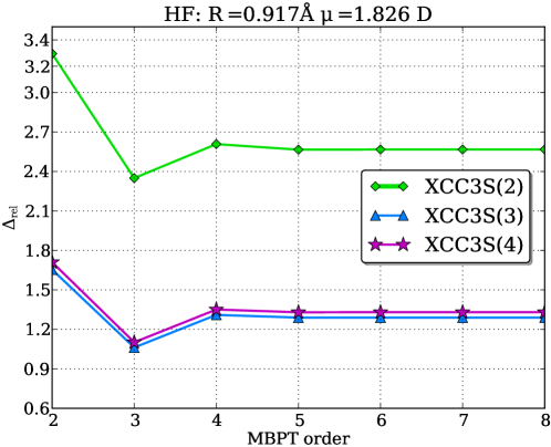
Figure 1: Reprinted from Ref [70] with permission of AIP Publishing (Figure 1, page 124109-5). The dipole moment of the HF molecule. The unsigned percentage error is defined as $\Delta_{\mathrm{rel}}$ $=$ $|\delta\mu|/|\mu_{\mathrm{exp}}|\times 100\%$. MBPT order corresponds to Table 3.

For all three approximations of $S$, the convergence of $\bar{X}$ is achieved after inclusion of the 5th order terms. To conclude, the convergence with respect to the $S$ operator approximation is achieved at the XCC3S(3) level and within that approximation the commutator terms of Table 3 need to be included up to the 5th order. More numerical results for dipole and quadrupole moments and comparison to the experimental data can be found in Ref [70].

2.4 Ground-state two-particle density matrix cumulant

The expression for the expectation value of an observable, Eq. (20), can be further used to obtain the coupled cluster parameterized density matrix cumulants. In the context of the coupled cluster theory, the cumulants appear for the first time in the work of Shork and Fuelde.[76] This subject was thoroughly studied some time later by Kutzelnigg and Mukherjee. [77, 78] Korona[79] investigated the parametrization of the two-particle density matrix cumulant employing the operator $S$.

The reduced one- and two-electron density matrix elements are defined in a given spinorbital basis as

$$\Gamma(\mathbf{x}_{1}|\mathbf{x}_{1}^{\prime})=\sum_{pq}\Gamma^{p}_{q}\phi_{p}^{*}(\mathbf{x}_{1})\phi_{q}(\mathbf{x}_{1}^{\prime})$$ (48)

$$\Gamma(\mathbf{x}_{1}\mathbf{x}_{2}|\mathbf{x}_{1}^{\prime}\mathbf{x}_{2}^{\prime})=\sum_{pqrs}\Gamma^{pr}_{qs}\phi_{p}^{*}(\mathbf{x}_{1})\phi_{r}^{*}(\mathbf{x}_{2})\phi_{q}(\mathbf{x}_{1}^{\prime})\phi_{s}(\mathbf{x}_{2}^{\prime})$$ (49)

where the expansion coefficients are

$$\Gamma^{p}_{q}=\braket{\Psi}{e^{p}_{q}\Psi}$$ (50)

$$\Gamma^{pr}_{qs}=\braket{\Psi}{e^{pr}_{qs}\Psi}.$$ (51)

The two-particle density matrix (2-RDM) $\Gamma^{pr}_{qs}$ can be rewritten in the following way [77]

$$\Gamma^{pr}_{qs}=\Gamma^{p}_{q}\Gamma^{r}_{s}-\Gamma^{p}_{s}\Gamma^{r}_{q}+\Lambda^{pr}_{qs},$$ (52)

where the first two terms on the r.h.s. of the above equation are products of one-electron density matrices and the last term is the matrix element of the cumulant. In contrast to the 2-RDM, its cumulant is size-extensive.[77] Starting from the XCC formulation of the two-electron density matrix,[65] we can write

$$\Gamma^{pr}_{qs}=\braket{e^{S^{\dagger}}e^{-T}e^{pr}_{qs}e^{T}e^{-S^{\dagger}}},$$ (53)

using the relation[80]

$$e^{pr}_{qs}=e^{p}_{q}e^{r}_{s}-\delta_{rq}e^{p}_{s},$$ (54)

and the equalities b and d of Table 1, we obtain the the expression

$$\Gamma^{pr}_{qs}=\braket{e^{S^{\dagger}}e^{-T}e^{p}_{q}e^{T}e^{-S^{\dagger}}e^{S^{\dagger}}e^{-T}e^{r}_{s}e^{T}e^{-S^{\dagger}}}-\delta_{rq}\braket{e^{S^{\dagger}}e^{-T}e^{p}_{s}e^{T}e^{-S^{\dagger}}}.$$ (55)

This expression can by further reformulated to resemble Eq. (52)

$$\begin{split}\Gamma^{pr}_{qs}&=\braket{e^{S^{\dagger}}e^{-T}e^{p}_{q}e^{T}e^{-S^{\dagger}}}\braket{e^{S^{\dagger}}e^{-T}e^{r}_{s}e^{T}e^{-S^{\dagger}}}\\ &-\braket{e^{S^{\dagger}}e^{-T}e^{p}_{r}e^{T}e^{-S^{\dagger}}}\braket{e^{S^{\dagger}}e^{-T}e^{q}_{s}e^{T}e^{-S^{\dagger}}}\\ &+\braket{e^{S^{\dagger}}e^{-T}e^{p}_{q}e^{T}e^{-S^{\dagger}}\hat{\mathscr{P}}(e^{S^{\dagger}}e^{-T}e^{r}_{s}e^{T}e^{-S^{\dagger}})}\\ &-\braket{e^{S^{\dagger}}e^{-T}\tilde{e}^{r}_{q}e^{T}e^{-S^{\dagger}}}\braket{e^{S^{\dagger}}e^{-T}e^{p}_{s}e^{T}e^{-S^{\dagger}}},\end{split}$$ (56)

where $\tilde{e}^{r}_{q}$ are one-hole substitution operators.[80] One can recognize the first two terms of Eq. (56) as the products of one-electron density matrix elements present in Eq. (52). The last two terms of Eq. (56), define the XCC cumulant of the two-electron density matrix

$$\Lambda^{pr}_{qs}=\braket{e^{S^{\dagger}}e^{-T}e^{p}_{q}e^{T}e^{-S^{\dagger}}\hat{\mathscr{P}}(e^{S^{\dagger}}e^{-T}e^{r}_{s}e^{T}e^{-S^{\dagger}})}\\ -\braket{e^{S^{\dagger}}e^{-T}\tilde{e}^{r}_{q}e^{T}e^{-S^{\dagger}}}\braket{e^{S^{\dagger}}e^{-T}e^{p}_{s}e^{T}e^{-S^{\dagger}}}.$$ (57)

In contrast to the expression for the XCC expectation value, Eq. (25), it is not obvious that the XCC cumulant $\Lambda^{pr}_{qs}$ is connected. Korona proved[79] that some parts of the first term in Eq. (57) cancel out the disconnected term. Therefore, we can write

$$\Lambda^{pr}_{qs}=\braket{\{e^{S^{\dagger}}e^{-T}e^{p}_{q}e^{T}e^{-S^{\dagger}}\hat{\mathscr{P}}(e^{S^{\dagger}}e^{-T}e^{r}_{s}e^{T}e^{-S^{\dagger}})\}_{C}},$$ (58)

where the subscript $C$ means that one has to consider only the connected terms.

The XCC approach was employed in reference SAPT theory[81, 82] calculations of Korona et. al.[72] A modified version of the first-order exchange energy formula[68] of SAPT was divided into two parts. The first one was expressed through the one-electron density matrices and the second part through the monomer cumulants. In this method, both monomers are described at the CCSD level. Numerical results and extensive discussion can be found in the paper by Korona.[72]

3 Time-independent coupled cluster theory of the polarization propagator

In this section we concentrate on the linear coefficient $\braket{\braket{X;Y}}_{\omega}$ in the expansion of the time-dependent expectation value of the operator $X$ from Eq. (14). The linear response function is also known as the polarization propagator and was derived in time-independent approach with the use of the auxiliary operator $S$ by Moszynski et. al.[66] The polarization propagator can be written down as[11]

$$\braket{\braket{X;Y}}_{\omega}=-\braket{\Psi_{0}}{Y\frac{Q}{H-E_{0}+\omega}X\Psi_{0}}-\braket{\Psi_{0}}{X\frac{Q}{H-E_{0}-\omega}Y\Psi_{0}},$$ (59)

where $Q=1-\ket{\Psi_{0}}\bra{\Psi_{0}}$ is the projection operator on the space spanned by all excited states. For Hermitian operators X and Y the second term in the above equation can be obtained by computing the first term for $-\omega^{*}$. This operation, called the generalized complex conjugation, is usually denoted as g.c.c. The propagator exhibits the following Hermitian symmetry

$$\braket{\braket{X;Y}}_{\omega}^{*}=\braket{\braket{X;Y}}_{-\omega^{*}}.$$ (60)

Introducing the first-order wavefunction $\Psi^{(1)}(\omega)$

$$(H-E_{0}-\omega)\Psi^{(1)}(\omega)=-X\Psi_{0}$$ (61)

the polarization propagator can be rewritten as

$$\langle\langle X;Y\rangle\rangle_{\omega}=-\braket{\Psi_{0}}{Y-\bar{Y}}{\Psi^{(1)}(\omega)}+\text{g.c.c.}$$ (62)

$\Psi^{(1)}(\omega)$ parametrized with the excitation operator $\Omega(\omega)=\Omega_{1}(\omega)+\Omega_{2}(\omega)+\ldots$, takes the form

$$|\Psi^{(1)}(\omega)\rangle=(\Omega_{0}(\omega)+\Omega(\omega))|\Psi_{0}\rangle.$$ (63)

$\Omega_{0}(\omega)$ is a scalar term that ensures the orthogonality of $\Psi^{(1)}$ to $\Psi_{0}$[66, 24]

$$\Omega_{0}(\omega)=-\braket{\Psi_{0}}{\Omega(\omega)\Psi_{0}},$$ (64)

and the amplitudes $\Omega_{n}(\omega)$ are the solutions of the linear-response equation [66, 24]

$$\left\langle\mu_{n}|[e^{-T}He^{T},\Omega(\omega)]+\omega\Omega(\omega)+e^{-T}Xe^{T}\right\rangle=0.$$ (65)

Upon inserting the CC parametrized $\Psi^{(1)}(\omega)$ and normalized CC ground state wavefunction $\Psi_{0}$[66]

$$\Psi_{0}=\frac{e^{T}}{\braket{e^{T^{\dagger}}e^{T}}^{\frac{1}{2}}}\Phi,$$ (66)

the first term on the r.h.s. of Eq. (62) becomes

$$\braket{\Psi_{0}}{(Y-\bar{Y})\Psi^{(1)}(\omega)}=\frac{\braket{e^{T}}{Y}{\Omega(\omega)e^{T}}}{\braket{e^{T}}{e^{T}}}-\bar{Y}\frac{\braket{e^{T}}{\Omega(\omega)e^{T}}}{\braket{e^{T}}{e^{T}}},$$ (67)

and using the formulas b and d from Table 1 one arrives at

$$\braket{\Psi_{0}}{(Y-\bar{Y})\Psi^{(1)}(\omega)}=\\ \braket{e^{-S}e^{T^{\dagger}}Ye^{-T^{\dagger}}e^{S}}{e^{S^{\dagger}}\Omega(\omega))e^{-S^{\dagger}}}\\ -\braket{e^{-S}e^{T^{\dagger}}Ye^{-T^{\dagger}}e^{S}}\braket{e^{S^{\dagger}}\Omega(\omega)e^{-S^{\dagger}}}.$$ (68)

Similarly as in the case of the cumulant, the last term in the above formula is explicitly disconnected and therefore some parts of the first term cancel out the second term on the r.h.s. This is demonstrated by using formula c from Table 1 in the work of Moszynski et. al.[66] so the polarization propagator takes the form

$$\langle\langle X;Y\rangle\rangle_{\omega}=\braket{e^{-S}e^{T^{\dagger}}Ye^{-T^{\dagger}}e^{S}}{\hat{\mathscr{P}}\left(e^{S^{\dagger}}\Omega(\omega)e^{-S^{\dagger}}\right)}+\text{g.c.c.}$$ (69)

The XCC formulation of the linear response function is size-consistent as it is expressed solely in terms of commutators. It is worth noting that the XCC polarization propagator exhibits the Hermitian symmetry, Eq. (60), in contrast to the TD-CC polarization propagator. The a posteriori symmetrization[54, 83] of the latter recovers the missing term with the wrong coefficient.[66, 24]

3.1 MBPT expansion

Moszynski and Jeziorski[66] proposed both perturbative and non-perturbative schemes of approximating $\braket{\braket{X;Y}}_{\omega}$ within the CCSD model. In the former approach the $T$ and $S$ amplitudes are found in the same way as in Section 2.1. The order-by-order expressions for $\Omega_{n}$ are computed from the linear response equation which can be rewritten as

$$\Omega_{n}(\omega)=\hat{\mathscr{R}}_{n,\omega}(e^{-T}Xe^{T}+[e^{-T}We^{T},\Omega(\omega)]),$$ (70)

where

$$\mathscr{\hat{R}}_{{n},\omega}(W)=\frac{1}{(n!)^{2}}\sum_{a_{n}i_{n}}\frac{\braket{e^{i_{1}\ldots i_{n}}_{a_{1}\ldots a_{n}}W}e_{i_{1}\ldots i_{n}}^{a_{1}\ldots a_{n}}}{(\epsilon_{i_{1}}+\ldots+\epsilon_{i_{n}}-\epsilon_{a_{1}}-\ldots-\epsilon_{a_{n}})-\omega}.$$ (71)

is the frequency-dependent resolvent. Therefore, in the first two orders of MBPT, the contributions to $\Omega_{n}$ are given by

$$\Omega_{1}^{(0)}= \mathscr{\hat{R}}_{{1},\omega}(X)$$ (72)

$$\Omega_{n}^{(1)}= \mathscr{\hat{R}}_{{n},\omega}([X,T_{2}^{(1)}]+[W,\Omega_{1}^{(0)}(\omega)]),\qquad n=1,2$$

$$\Omega_{n}^{(2)}= \mathscr{\hat{R}}_{{n},\omega}([X,T_{1}^{(2)}+T_{2}^{(2)}]+$$

$$[W,\Omega_{1}^{(1)}(\omega)+\Omega_{2}^{(1)}(\omega)]+[[W,T_{2}^{(1)}],\Omega_{1}^{(0)}(\omega)]),\qquad n=1,2,3$$

and the polarization propagator itself is given by

$$\braket{\braket{X;Y}}_{\omega}^{(0)}=\braket{Y}{\Omega^{(0)}(\omega)}+\mbox{g.c.c.}$$ (73)

$$\braket{\braket{X;Y}}_{\omega}^{(1)}=\braket{Y}{{\Omega}_{1}^{(1)}(\omega)}+\braket{[Y,{T}_{2}^{(1)}]}{{\Omega}_{1}^{(0)}(\omega)}+\mbox{g.c.c.}$$

$$\braket{\braket{X;Y}}_{\omega}^{(2)}=\braket{Y}{{\Omega}_{1}^{(2)}(\omega)}+\braket{[Y,{T}_{2}^{(1)}]}{{\Omega}_{1}^{(1)}(\omega)}$$

$$+\braket{[Y,{T}_{2}^{(1)}]}{{\Omega}_{2}^{(1)}(\omega)}+\braket{[Y,{T}_{1}^{(2)}]}{{\Omega}_{1}^{(0)}(\omega)}$$

$$+\braket{[Y,{T}_{2}^{(2)}]}{{\Omega}_{1}^{(0)}(\omega)}-\braket{[[Y,T_{2}^{(1)\dagger}],{T}_{2}^{(1)}]}{{\Omega}_{1}^{(0)}(\omega)}+\mbox{g.c.c.}$$

3.2 Expansion in powers of $T$

In the non-perturbative approximation, the $T$ amplitudes are computed from the conventional CC method, and the $S$ amplitudes are expanded in powers of $T$ in the same way as in Section 2.2. The solution of Eq. (65) for the $\Omega(\omega)$ operator is a standard procedure used to compute coupled cluster gradients.[50, 84, 85] Finally, the expression for the $\braket{\braket{X;Y}}_{\omega}$ itself is given through the combined powers of $T$ and $S$ operators. In the CCSD case one obtains

$$\braket{\braket{X;Y}}_{\omega}^{[0]}=\braket{Y}{\Omega_{1}(\omega)}+\mbox{g.c.c.}$$ (74)

$$\braket{\braket{X;Y}}_{\omega}^{[1]}=\braket{S}{[Y,\Omega(\omega)]}+\braket{[Y,S_{2}]}{\Omega_{1}(\omega)}+\mbox{g.c.c.}$$

$$\braket{\braket{X;Y}}_{\omega}^{[2]}=-\braket{[[Y,T^{\dagger}],S]}{\Omega(\omega)}+\braket{[Y,S]}{[S_{1}^{\dagger},\Omega_{2}(\omega)]}$$

$$+\frac{1}{2}\braket{[[Y,S],S]}{\Omega(\omega)}+\mbox{g.c.c.}$$

$$\braket{\braket{X;Y}}_{\omega}^{[3]}=-\frac{1}{2}\braket{[[[Y,T^{\dagger}],S],S]}{\Omega(\omega)}-\braket{[[Y,T^{\dagger}],S]}{[S_{1}^{\dagger},\Omega_{2}(\omega)}$$

$$+\frac{1}{2}\braket{[[[Y,T_{1}^{\dagger}],T_{1}^{\dagger}],S_{2}}{\Omega_{1}(\omega)}+\frac{1}{2}\braket{[[Y,S_{1}],S_{1}]}{[S_{1}^{\dagger},\Omega_{2}(\omega)}+\mbox{g.c.c.}$$

The XCC method for the polarization propagator was implemented by Korona et al.[24, 25, 69] and a highly-optimized implementation is available in the Molpro software package.[86] In the XCC algorithm $\Omega(\omega)$ is obtained in an iterative procedure, and each iteration scales as $\mathscr{O}(o^{2}v^{4})$. The calculation of $\Omega(\omega)$ is the most expensive part. Computation of $S$ amplitudes and the polarization propagator, are one-step procedures, and scale up to $\mathscr{O}(o^{3}v^{3})$. In TD-CC method one must also compute the $\Lambda$ state, which is of similar cost as computing $\Omega(\omega)$. Therefore this method is twice as expensive than XCC method.

As the first application the polarization propagator was used to compute static and dynamic electric dipole polarizabilities[24] of various molecules such as H₂, He, Be, BH, CH⁺, Ne and HF. The results were compared with the FCI method and it was confirmed numerically, that the method is almost exact for two-electron systems.[66, 24] The only approximation originates from an inexact treatment of the $S$ amplitudes, where some of the multiply-nested commutators were neglected.

The XCC formulation of the polarization propagator was also used to compute the second order dispersion energy $E^{(2)}_{\mbox{\tiny{disp}}}$ within the SAPT framework.[69] The Longuet-Higgins formula for

$$E^{(2)}_{\mbox{\tiny{disp}}}=-\frac{1}{2\pi}\int_{0}^{\infty}\int\int\int\alpha^{A}(\mathbf{r}_{1},\mathbf{r}_{2}|i\omega)\alpha^{B}(\mathbf{r}_{3},\mathbf{r}_{4}|i\omega)\frac{1}{r_{13}}\frac{1}{r_{24}}d\mathbf{r}_{1}d\mathbf{r}_{2}d\mathbf{r}_{3}d\mathbf{r}_{4}$$ (75)

is expressed through frequency-dependent density susceptibilities

$$\alpha^{A}(\mathbf{r}_{1},\mathbf{r}_{2}|\omega)=\braket{\braket{\hat{\rho}(\mathbf{r}_{1});\hat{\rho}(\mathbf{r}_{1})}}_{\omega}.$$ (76)

One can show that $\alpha^{A}(\mathbf{r}_{1},\mathbf{r}_{2}|i\omega)$ is obtained from the polarization propagator $\braket{\braket{X;Y}}_{\omega}$ where both $X$ and $Y$ are the electron density operators

$$\hat{\rho}(\mathbf{r}_{1})=\sum_{i=1}^{N}\delta(\mathbf{r}-\mathbf{r}_{i}).$$ (77)

In order to lower the computational cost, Korona and Jeziorski[69] used the density fitting method[87, 88, 89] for the computation of the density susceptibilities.

3.3 First-order density matrix cumulant

The XCC formalism was adapted for the computation of the second-order exchange-induction energy of SAPT theory.[73] The $E_{\mbox{\tiny{exch-ind}}}^{(2)}$ is defined in the $S^{2}$ approximation, as[90]

$$E_{\mbox{\tiny{exch-ind}}}^{(2)}=\braket{\Psi_{A}\Psi_{B}}{(V-\bar{V})(P-\bar{P})(\Psi^{(1)}_{A}\Psi_{B}+\Psi_{A}\Psi^{(1)}_{B})},$$ (78)

where $V$ is the intermolecular potential, and $P=-\sum_{i=1}^{N_{A}}\sum_{j=1}^{N_{B}}P_{ij}$ is a single-exchange operator. The authors of Ref [73] express $E_{\mbox{\tiny{exch-ind}}}^{(2)}$ through 1-RDM and 2-RDM of monomers and subsequently divide the resulting expression in the antisymmetrized product of 1-RDMs part and the cumulant part.

The first-order density matrix element is defined as

$$(\Gamma^{(1)})^{pr}_{qs}=\braket{\Psi_{0}}{e^{pr}_{qs}\Psi^{(1)}}.$$ (79)

To obtain the coupled cluster parametrization of this quantity, one uses the $\Psi_{0}$ and $\Psi_{1}$, Eq. (66) and Eq. (63), and takes $\omega=0$. Inserting the definition of the $S$ operator Eq. (19), gets[73]

$$\braket{\Psi_{0}}{X\Psi^{(1)}}=\Omega_{0}\braket{e^{S^{\dagger}}e^{-T}Xe^{T}}+\braket{e^{S^{\dagger}}e^{-T}X\Omega e^{T}}.$$ (80)

Further steps require to use the formulas from Table 1

$$\braket{\Psi_{0}}{X\Psi^{(1)}}=-\braket{e^{S^{\dagger}}\Omega e^{-S^{\dagger}}}\braket{e^{S^{\dagger}}e^{-T}Xe^{T}e^{-S^{\dagger}}}+\\ \braket{e^{S^{\dagger}}e^{-T}Xe^{T}e^{-S^{\dagger}}}\braket{e^{S^{\dagger}}\Omega e^{-S^{\dagger}}}+\braket{e^{S^{\dagger}}e^{-T}Xe^{T}e^{-S^{\dagger}}\hat{\mathscr{P}}(e^{S^{\dagger}}\Omega e^{-S^{\dagger}})},$$ (81)

where in first term $\Omega_{0}$ is replaced with $-\braket{e^{S^{\dagger}}\Omega e^{-S^{\dagger}}}$. The first-order density matrix becomes

$$(\Gamma^{(1)})^{pr}_{qs}=\braket{\Psi}{e^{pr}_{qs}\Psi^{(1)}}=\braket{e^{S^{\dagger}}e^{-T}e^{pr}_{qs}e^{T}e^{-S^{\dagger}}\hat{\mathscr{P}}(e^{S^{\dagger}}\Omega e^{-S^{\dagger}})}.$$ (82)

The first-order cumulant $\Lambda^{(1)}$ of the first-order 2-RDM is defined as

$$(\Gamma^{(1)})^{pr}_{qs}=(\Gamma^{(1)})^{p}_{q}(\Gamma^{(0)})^{r}_{s}+(\Gamma^{(0)})^{p}_{q}(\Gamma^{(1)})^{r}_{s}\\ -(\Gamma^{(1)})^{p}_{s}(\Gamma^{(0)})^{r}_{q}-(\Gamma^{(0)})^{p}_{s}(\Gamma^{(1)})^{r}_{q}+(\Lambda^{(1)})^{pr}_{qs}.$$ (83)

Korona[73] showed how to divide Eq. (82) in order to identify the first-order cumulant. The formula c from Table 1 is inserted between any pair of operators so the Eq. (68) becomes

$$(\Gamma^{(1)})^{pr}_{qs}=\langle e^{S^{\dagger}}e^{-T}p^{\dagger}e^{T}e^{-S^{\dagger}}e^{S^{\dagger}}e^{-T}r^{\dagger}e^{T}e^{-S^{\dagger}}e^{S^{\dagger}}e^{-T}q\times\\ \times e^{T}e^{-S^{\dagger}}e^{S^{\dagger}}e^{-T}se^{T}e^{-S^{\dagger}}\hat{\mathscr{P}}(e^{S^{\dagger}}\Omega e^{-S^{\dagger}})\rangle,$$ (84)

and introducing the shorthand notation

$$\Theta=\hat{\mathscr{P}}(e^{S^{\dagger}}\Omega e^{-S^{\dagger}})$$ (85)

$$K^{p}=e^{S^{\dagger}}e^{-T}p^{\dagger}e^{T}e^{-S^{\dagger}}$$

$$R_{q}=e^{S^{\dagger}}e^{-T}qe^{T}e^{-S^{\dagger}}$$

one obtains an expression for $(\Gamma^{(1)})^{pr}_{qs}$

$$(\Gamma^{(1)})^{pr}_{qs}=\braket{\{K^{p}K^{r}R_{s}R_{q}\Theta\}_{C}}+\braket{K^{p}R_{q}}\braket{K^{r}R_{s}\Theta}+\\ \braket{K^{r}R_{s}}\braket{K^{p}R_{q}\Theta}-\braket{K^{r}R_{q}}\braket{K^{p}R_{s}\Theta}-\braket{K^{p}R_{s}}\braket{K^{r}R_{q}\Theta},$$ (86)

where subscript C denotes taking only the connected part of the term. The cumulant is identified as the first term on the r.h.s. of the above equation

$$(\Lambda^{(1)})^{pr}_{qs}=\braket{\{K^{p}K^{r}R_{s}R_{q}\Theta\}_{C}},$$ (87)

by comparison of the Eq. (86) and Eq. (83). This approach allows one to include the intramonomer correlation at the CCSD level for the many-electron monomers.

3.4 Transition moments from ground to excited states

The natural step to further develop the XCC theory is to derive the expressions for the transition moments. Transition moments from ground to excited electronic states can be found as a residue of the polarization propagator. In the exact theory, one can write the transition moments between the ground and an excited state $K$ as

$$\lim_{\omega\rightarrow\omega_{K}}(\omega-\omega_{K})\braket{\braket{X;Y}}_{\omega}=\braket{\Psi_{0}}{X\Psi_{K}}\braket{\Psi_{K}}{Y\Psi_{0}}=T_{X}^{0K}T_{Y}^{K0}.$$ (88)

The product $T_{X}^{0K}T_{Y}^{K0}$ is called the transition strength matrix and satisfies the condition

$$\mathcal{S}_{XY}^{0K}=-(\mathcal{S}_{XY}^{K0})^{*},$$ (89)

which is a direct consequence of the Hermitian symmetry of the polarization propagator.[66]

In the XCC theory the excited states are obtained from the equation of motion coupled cluster theory (EOM-CC) using CC Jacobian,[91, 53, 92] which has the following form

$$A_{\mu_{n}\nu_{m}}=\frac{d\braket{\mu_{n}}{e^{-T}He^{T}}{\Phi}}{d\nu_{m}}=\braket{\mu_{n}}{e^{-T}[H,\nu_{m}]e^{T}}{\Phi}.$$ (90)

Due to the non-symmetric character of the Jacobian matrix, the diagonalization of $A$ leads to a set of biorthogonal left $l_{M}$ and right $r_{K}$ eigenvectors

$$\braket{l_{M}}{r_{K}}=\delta_{MK}.$$ (91)

The transformation to the Jacobian basis is given by

$$\mu_{n}=\sum_{N}L^{\star}_{\mu_{n}\mbox{\tiny{\emph{N}}}}r_{N},$$ (92)

and is used to express the operator $\Omega(\omega)$ in terms of the Jacobian eigenvectors

$$\Omega^{X}(\omega)=\sum_{M}\sum_{n}\sum_{\nu_{n}}L_{\nu_{n}M}^{*}O_{\nu_{n}}^{X}(\omega)r_{M}=\sum_{M}O_{M}^{X}(\omega)r_{M}.$$ (93)

Inserting Eq. (93) to the linear response equation for $\Omega(\omega)$, Eq. (65), one obtains

$$\sum_{M}\braket{l_{N}}{e^{-T}[H,r_{M}]e^{T}}O_{M}^{X}(\omega)+\sum_{M}\omega\braket{l_{N}}{r_{M}}O_{M}^{X}(\omega)+\braket{l_{N}}{e^{-T}Xe^{T}}=0,$$ (94)

where we use the superscript $X$ to indicate the $X$ dependence. Eq. (94) can be simplified to the following form using the facts that the Jacobian matrix is diagonal in this basis, and that this basis is biorthonormal

$$\braket{l_{N}}{e^{-T}[H,r_{N}]e^{T}}O_{N}^{X}(\omega)+\omega O_{N}^{X}(\omega)+\braket{l_{N}}{e^{-T}Xe^{T}}=0.$$ (95)

Denoting $\braket{l_{N}}{e^{-T}[H,r_{N}]e^{T}}$ as the nth excitation energy $\omega_{N}=E_{N}-E_{0}$, Eq. (95) can be rewritten as

$$\omega_{N}O_{N}^{X}(\omega)+\omega O_{N}^{X}(\omega)+\xi_{N}^{X}=0$$ (96)

where

$$\xi_{N}^{X}=\braket{l_{N}}{e^{-T}Xe^{T}}.$$ (97)

The quantity $O_{N}^{X}(\omega)$ is then straightforwardly obtained as

$$O_{N}^{X}(\omega)=-\frac{\xi_{N}^{X}}{\omega_{N}+\omega}.$$ (98)

Eq. (69) is transformed to the Jacobian basis according to the following steps

$$\langle\langle X;Y\rangle\rangle_{\omega}=\braket{e^{-S}e^{T^{\dagger}}Ye^{-T^{\dagger}}e^{S}}{\hat{\mathscr{P}}(e^{S^{\dagger}}\Omega^{X}(\omega)e^{-S^{\dagger}})}+\mbox{g.c.c.}=\\ \sum_{n=1}\sum_{\mu_{n}}O^{X}_{\nu_{n}}\braket{e^{-S}e^{T^{\dagger}}Ye^{-T^{\dagger}}e^{S}}{\hat{\mathscr{P}}(e^{S^{\dagger}}\tau_{\mu_{n}}e^{-S^{\dagger}})}+\mbox{g.c.c.}=\\ \sum_{N}O^{X}_{N}\braket{e^{-S}e^{T^{\dagger}}Ye^{-T^{\dagger}}e^{S}}{\hat{\mathscr{P}}(e^{S^{\dagger}}r_{N}e^{-S^{\dagger}})}+\mbox{g.c.c.}$$ (99)

Using Eq. (98) and denoting

$$\gamma_{N}^{Y}=\braket{e^{-S}e^{T^{\dagger}}Ye^{-T^{\dagger}}e^{S}}{\hat{\mathscr{P}}(e^{S^{\dagger}}r_{N}e^{-S^{\dagger}})},$$ (100)

the XCC linear response function in the Jacobian eigenvector basis becomes

$$\langle\langle X;Y\rangle\rangle_{\omega}=-\sum_{N}\frac{\xi_{N}^{X}\gamma_{N}^{Y}}{\omega_{N}+\omega}+\mbox{g.c.c.}$$ (101)

The poles of Eq. (101) are located at the EOM-CC[93] excitation energies, and the residue of the XCC response function reads

$$\lim_{\omega\rightarrow-\omega_{K}}(\omega+\omega_{K})\braket{\braket{X;Y}}_{\omega}=-\underbrace{\gamma_{K}^{Y}}_{T_{Y}^{0K}}\underbrace{\xi_{K}^{X}}_{T_{X}^{K0}}=\mathcal{S}_{XY}^{0K}.$$ (102)

The line strength $\mathcal{S}_{XY}^{0K}$ is exclusively expressed in terms of commutators, and is automatically size consistent, regardless of any truncation of the $T$ and $S$ operators. The XCC transition strength satisfies the antihermiticity relation Eq. (89) for any truncation of the operator $T$. The situation is more complicated for the truncated operator $S$. In the derivations we have used the formal definition of the operator $S$, $e^{S}\Phi=\frac{e^{T^{\dagger}}e^{T}}{\braket{e^{T}}{e^{T}}}\Phi$, which is true only for the exact $S$. Nonetheless, the deviations from the exact Hermitian symmetry are numerically negligible.[70, 71] This issue is discussed in more detail in the next section. The numerical results computed by Tucholska et al.[70] covers the dipole and quadrupole transition probabilities for the Mg, Ca, Sr and Ba atoms, comparison to the TD-CC method and experimental data.

4 Quadratic response function

The next coefficient in the expansion given by Eq. (14) is the quadratic response function, $\braket{\braket{X;Y,Z}}_{\omega_{Y},\omega_{Z}}$. It describes a response of an observable $X$ to the perturbations $Y$ and $Z$ acting with the frequencies $\omega_{Y}$ and $\omega_{Z}$, respectively, and is defined as the following sum over states [44]

$$\langle\langle X;Y,Z\rangle\rangle {}_{\omega_{Y},\omega_{Z}}=$$ (103)

$$=P_{XYZ} \sum_{\begin{subarray}{c}K=1\\ N=1\end{subarray}}\frac{\braket{\Psi_{0}}{Y}{\Psi_{K}}[\braket{\Psi_{K}}{X}{\Psi_{N}}-\delta_{KN}\braket{\Psi_{0}}{X}{\Psi_{0}}]\braket{\Psi_{N}}{Z}{\Psi_{0}}}{(\omega_{K}+\omega_{Y})(\omega_{N}-\omega_{Z})},$$

where the operator $P_{XYZ}$ denotes the sum of all permutations of the indices $X$, $Y$ and $Z$. $K$ and $N$ run over all possible excited states with the excitation energies $\omega_{K}$ and $\omega_{N}$ and $\Psi_{0}$ is the ground state. By using the first-order perturbed wave function, Eq. (63), we rewrite Eq. (103) as

$$\braket{\braket{X;Y,Z}}_{\omega_{Y},\omega_{Z}}=P_{XYZ}\langle\Psi^{(1)}(\omega_{Y})|X_{0}|\Psi^{(1)}(-\omega_{Z})\rangle,$$ (104)

where we introduced the symbol $X_{0}=X-\braket{X}$. In the form parametrized by CC wavefunctions, the quadratic response function reads

$$\braket{\braket{X;Y,Z}}_{\omega_{Y},\omega_{Z}}=\\ P_{XYZ}\langle(\Omega_{0}(\omega_{Y})+\Omega(\omega_{Y}))\Psi_{0}|X_{0}|(\Omega_{0}(\omega_{Z})+\Omega(-\omega_{Z}))\Psi_{0}\rangle.$$ (105)

After expanding Eq. (105) and using the formulas from Table 1, we get the final expression for the quadratic response function in XCC formalism

$$\braket{\braket{X;Y,Z}}_{\omega_{Y},\omega_{Z}}=\\ P_{XYZ}\left(\braket{\hat{\mathscr{P}}(e^{S^{\dagger}}\Omega^{Y}e^{-S^{\dagger}})}{e^{-S}e^{T^{\dagger}}X_{0}e^{-T^{\dagger}}e^{S}\hat{\mathscr{P}}(e^{-S}e^{T^{\dagger}}\Omega^{Z}e^{-T^{\dagger}}e^{S})}\right).$$ (106)

4.1 Transition moments between excited states

A transition moment between two excited states is obtained from the residue of the quadratic response function. For the exact wavefunction the residue is

$$\lim_{\omega_{Y}\rightarrow-\omega_{L}}(\omega_{L}+\omega_{Y})\lim_{\omega_{Z}\rightarrow\omega_{M}}(\omega_{M}-\omega_{Z})\braket{\braket{X;Y,Z}}_{\omega_{Y},\omega_{Z}}$$ (107)

$$= \braket{\Psi_{0}}{Y}{\Psi_{L}}\braket{\Psi_{L}}{X_{0}}{\Psi_{M}}\braket{\Psi_{M}}{Z}{\Psi_{0}}=\mathcal{T}^{Y}_{0L}\mathcal{T}^{X}_{LM}\mathcal{T}^{Z}_{M0}.$$

By expanding Eq. (106) in the basis of the CC Jacobian eigenvectors Eq. (93), one gets

$$\braket{\braket{X;Y,Z}}_{\omega_{Y},\omega_{Z}}=P_{XYZ}\sum_{K,N=1}\left(O_{K}^{Y}(\omega_{Y})\right)^{\star}O_{N}^{Z}(-\omega_{Z})$$ (108)

$$\times\braket{\hat{\mathscr{P}}(e^{S^{\dagger}}r_{K}e^{-S^{\dagger}})}{e^{-S}e^{T^{\dagger}}X_{0}e^{-T^{\dagger}}e^{S}\hat{\mathscr{P}}(e^{-S}e^{T^{\dagger}}r_{N}e^{-T^{\dagger}}e^{S})}.$$

By introducing a shorthand notation for the projected parts of the above expression

$$\begin{split}&\kappa(r_{M},S,T)=\hat{\mathscr{P}}\left(e^{-S}e^{T^{\dagger}}r_{K}e^{-T^{\dagger}}e^{S}\right)\\ &\eta(r_{N},S)=\hat{\mathscr{P}}\left(e^{S^{\dagger}}r_{N}e^{-S^{\dagger}}\right),\end{split}$$ (109)

one arrives at the final form of the XCC quadratic response function in the Jacobian eigenvector basis

$$\braket{\braket{X;Y,Z}}_{\omega_{Y},\omega_{Z}}=$$ (110)

$$P_{XYZ}\sum_{\begin{subarray}{c}K=1\\ N=1\end{subarray}}\left(O_{K}^{Y}(\omega_{Y})\right)^{\star}O_{N}^{Z}(-\omega_{Z})\braket{\kappa(r_{K},S,T)}{e^{S^{\dagger}}e^{-T}X_{0}e^{T}e^{-S^{\dagger}}\eta(r_{N},S)}$$

$$=P_{XYZ}\sum_{\begin{subarray}{c}K=1\\ N=1\end{subarray}}\frac{\braket{e^{-T}Ye^{T}}{l_{K}}}{\omega_{K}+\omega_{Y}}\frac{\braket{l_{N}}{e^{-T}Ze^{T}}}{\omega_{Z}-\omega_{N}}\braket{\kappa(r_{K},S,T)}{e^{S^{\dagger}}e^{-T}X_{0}e^{T}e^{-S^{\dagger}}}{\eta(r_{N},S)}.$$

The residue of the XCC quadratic response function reads

$$\mathcal{T}_{0L}^{Y} \mathcal{T}_{LM}\mathcal{T}^{Z}_{M0}=\lim_{\omega_{Y}\rightarrow-\omega_{L}}(\omega_{L}+\omega_{Y})\lim_{\omega_{Z}\rightarrow\omega_{M}}(\omega_{M}-\omega_{Z})\braket{\braket{X;Y,Z}}_{\omega_{Y},\omega_{Z}}$$ (111)

$$=\braket{e^{-T}Ye^{T}}{l_{L}}\braket{\kappa(r_{L},S,T)}{e^{S^{\dagger}}e^{-T}X_{0}e^{T}e^{-S^{\dagger}}}{\eta(r_{M},S)}\braket{l_{M}}{e^{-T}Ze^{T}}.$$

It is important to notice that one obtains an approximation to the product $\mathcal{T}_{0L}^{Y}\mathcal{T}_{LM}\mathcal{T}^{Z}_{M0}$ rather than an expression for $\mathcal{T}_{LM}$. To single out the $\mathcal{T}_{LM}$ transition moment, we divide the whole quantity Eq. (111) by the product of the left and right transition moments from the ground state. These are obtained from the residue of $\langle\Psi^{(1)}(\omega_{Y})|X|\Psi^{(1)}(-\omega_{Z})\rangle$ with $L=M$ and $Y=Z$ and $X=1$. For the exact quadratic response function this quantity is simply $|T_{0L}^{Y}|^{2}=\braket{\Psi_{0}}{Y}{\Psi_{L}}\braket{\Psi_{L}}{Y}{\Psi_{0}}$, and thus can be used to extract the transition moment between the excited states. In the XCC theory, $|T_{0L}^{Y}|^{2}$ is a product of three integrals

$$|T_{0L}^{Y}|^{2}=\braket{e^{-T}Ye^{T}}{l_{L}}\braket{\kappa(r_{L},S,T)}{\eta(r_{L},S)}\braket{l_{L}}{e^{-T}Ye^{T}}.$$ (112)

As the final result, the residue of the quadratic response function in the XCC theory divided by $|\mathcal{T}_{0L}^{Y}\mathcal{T}_{M0}^{Z}|=\sqrt{|T_{0L}^{Y}|^{2}|T_{M0}^{Z}|^{2}}$ is given by the expression

$$\begin{split}\mathcal{T}_{LM}&=\pm\frac{\lim\limits_{\footnotesize{\omega_{Y}\rightarrow-\omega_{L}}}(\omega_{L}+\omega_{Y})\lim\limits_{\omega_{z}\rightarrow\omega_{M}}(\omega_{M}-\omega_{Z})\braket{\braket{X;Y,Z}}_{\omega_{Y},\omega_{Z}}}{\sqrt{|T_{0L}^{Y}|^{2}|T_{M0}^{Z}|^{2}}}\\[10.0pt] &=\pm\frac{\xi_{L}^{Y}\braket{\kappa(r_{L},S,T)}{e^{S^{\dagger}}e^{-T}X_{0}e^{T}e^{-S^{\dagger}}\eta(r_{M},S)}\xi_{M}^{Z}}{\sqrt{\xi_{L}^{Y}\braket{\kappa(r_{L},S,T)}{\eta(r_{L},S)}(\xi_{L}^{Y})^{\star}\xi_{M}^{Z}\braket{\kappa(r_{M},S,T)}{\eta(r_{M},S)}(\xi_{M}^{Z})^{\star}}},\end{split}$$ (113)

where $\xi_{M}^{Z}$ is defined analogously as Eq. (97). The sign of $\mathcal{T}_{LM}^{X}$ is of concern because in practical applications one requires only the transition strengths, i.e., the products $\mathcal{T}^{X}_{LM}\mathcal{T}^{X}_{ML}$. The final expression for $T_{LM}$ in the XCC theory is given by

$$\mathcal{T}_{LM}=\frac{\braket{\kappa(r_{L},S,T)}{e^{S^{\dagger}}e^{-T}X_{0}e^{T}e^{-S^{\dagger}}\eta(r_{M},S)}}{\sqrt{\braket{\kappa(r_{L},S,T)}{\eta(r_{L},S)}\braket{\kappa(r_{M},S,T)}{\eta(r_{M},S)}}}.$$ (114)

The Hermiticity relation

$$\mathcal{T}^{X}_{LM}=(\mathcal{T}^{X}_{ML})^{*}$$ (115)

is satisfied for any truncation of $T$, but does not hold exactly for a truncated operator $S$. The violation of Eq. (115) was investigated numerically in Ref [71] and we present the results in Table 4 (Table VII in Ref [71]). For the excited-state transitions of the Mg atom it was found that the violation of Eq. (115) is numerically negligible and in the problematic cases does not lead to an unphysical results as in the TD-CC method.

Transition $\mathcal{T}_{LM}^{X}(\mathrm{TDCC})$ $(\mathcal{T}_{ML}^{X})^{\star}(\mathrm{TDCC})$ $\mathcal{T}_{LM}^{X}(\mathrm{XCC})$ $(\mathcal{T}_{ML}^{X})^{\star}(\mathrm{XCC})$ aug-cc-pVQZ[94] $3s4s\prescript{1}{}{\mbox{S}}-3s3p\prescript{1}{}{\mbox{P}}^{\circ}$ $4.30$ $4.26$ $4.00$ $4.01$ $3s4p\prescript{1}{}{\mbox{P}}^{\circ}-3s4s\prescript{1}{}{\mbox{S}}$ $8.39$ $8.30$ $8.36$ $8.36$ d-aug-cc-pVQZ[95, 96] $3s5s\prescript{1}{}{\mbox{S}}-3s4p\prescript{1}{}{\mbox{P}}^{\circ}$ $10.12$ $10.04$ $10.08$ $10.09$ $3s5s\prescript{1}{}{\mbox{S}}-3s3p\prescript{1}{}{\mbox{P}}^{\circ}$ $0.60$ $0.60$ $0.51$ $0.51$ $3s3d\prescript{1}{}{\mbox{D}}-3s3p\prescript{1}{}{\mbox{P}}^{\circ}$ $0.67$ $-0.40$ $1.40$ $1.43$ $3s4p\prescript{1}{}{\mbox{P}}-3s3d\prescript{1}{}{\mbox{D}}$ $-1.18$ $0.72$ $2.64$ $2.63$

Table 4: Reprinted from Ref [71] with permission of AIP Publishing (Table VII, page 034108-7). $\mathcal{T}_{LM}^{X}$ and $(\mathcal{T}_{ML}^{X})^{\star}$ computed with the TD-CC and XCC methods for the Mg atom.

Ref [71] also reports the lifetimes of singlet and triplet states for the Ca, Sr, and Ba atoms and presents a comparison against experimental data of the Gaussian[97, 98] and Slater[99] basis set implementations. The conclusions are that the use of the CC3 approximation combined with the STO basis sets give the results that show the smallest mean absolute percentage deviation from experimental data. Additionally the proof that the XCC transition moments are size intensive can be found Ref. [71].

5 Summary

We have presented a review of the expectation value method for the computation of ground-state properties, response properties, and transition probabilities within the coupled-cluster formalism. We summarized the derivations of the average value of an observable, one- and two-electron density matrices, polarization propagator, quadratic response function, and transition moments between the ground and excited states. The XCC formalism is conceptually simple and easily extendable to general operators: the calculation of a property requires only a single-step computation of the amplitudes of the auxiliary operator S that enter the definition of the average value. The methodology can easily be extended to the CC models other CCSD and CC3 provided that the set of commutators/contributions retained in the working formulas for the matrix elements properly corresponds to the choice of the ground state amplitudes. The computational cost of the XCC computation is controlled by the level of approximation of the operator S and the subset terms retained in the commutator expansion of the property value. The selection of included contributions is guided either by the MBPT expansion or powers of T. Both approaches yield a straightforward scheme of approximations that can be expanded to include higher excitations or to employ one of modern highly-efficient computational techniques developed for the ground-state coupled cluster theory. In particular, the simple formulation of the XCC method makes it possible to combine it with the explicitly correlated methods, which is a work underway in our laboratory. Further work related to the XCC theory concerns the description of the spin-orbit coupling matrix elements, magnetic moments, nonadiabatic coupling and open-shell systems.

6 Acknowledgment

We would like to thank Dr. M. Lesiuk and Dr. M. Modrzejewski for useful discussions regarding the manuscript. This research was supported by the National Science Center (NCN) under Grant No. 2017/25/B/ST4/02698.

References

• [1] I. Shavitt. The history and evolution of configuration interaction. Mol. Phys. 1998 94(1), pp 3–17.
• [2] J. Čížek. On the correlation problem in atomic and molecular systems. calculation of wavefunction components in ursell-type expansion using quantum-field theoretical methods. J. Chem. Phys. 1966 45(11), pp 4256–4266.
• [3] J. Čížek. On the use of the cluster expansion and the technique of diagrams in calculations of correlation effects in atoms and molecules. Adv. Chem. Phys. 1969 14 pp 35–89.
• [4] M. Motta, S. Zhang. Computation of ground-state properties in molecular systems: Back-propagation with auxiliary-field quantum Monte Carlo. J. Chem. Theory Comput. 2017 13(11), pp 5367–5378.
• [5] J. Vrbik, D. A. Legare, S. M. Rothstein. Infinitesimal differential diffusion quantum Monte Carlo: Diatomic molecular properties. J. Chem. Phys. 1990 92(2), pp 1221–1227.
• [6] R. E. Thomas, D. Opalka, C. Overy, P. J. Knowles, A. Alavi, G. H. Booth. Analytic nuclear forces and molecular properties from full configuration interaction quantum Monte Carlo. J. Chem. Phys. 2015 143(5), pp 054108.
• [7] S. R. White. Density matrix formulation for quantum renormalization groups. Phys. Rev. Lett. 1992 69(19), pp 2863.
• [8] S. R. White. Density-matrix algorithms for quantum renormalization groups. Phys. Rev. B 1993 48(14), pp 10345.
• [9] U. Schollwöck. The density-matrix renormalization group. Rev. Mod. Phys. 2005 77(1), pp 259.
• [10] B. Pickup Theory and computation of molecular properties in: Atomic and Molecular Properties Springer, 1992 pp 157–265.
• [11] J. Oddershede Polarization propagator calculations in: Adv. Quantum Chem. Vol. 11 Elsevier, 1978 pp 275–352.
• [12] J. Oddershede, P. Jørgensen, D. L. Yeager. Polarization propagator methods in atomic and molecular calculations. Comp. Phys. Rep. 1984 2(2), pp 33–92.
• [13] J. Oddershede. Propagator methods. Adv. Chem. Phys. 1987 69 pp 201–239.
• [14] J. Linderberg, Y. Öhrn Propagators in quantum chemistry John Wiley & Sons, 2004.
• [15] P. Jørgensen Second quantization-based methods in quantum chemistry Elsevier, 2012.
• [16] F. Coester. Bound states of a many-particle system. Nature Phys. 1958 7 pp 421–424.
• [17] F. Coester, H. Kümmel. Short-range correlations in nuclear wave functions. Nature Phys. 1960 17 pp 477–485.
• [18] C. Dykstra, G. Frenking, K. Kim, G. Scuseria Theory and Applications of Computational Chemistry: the first forty years Elsevier, 2011.
• [19] J. Paldus, J. Čížek, I. Shavitt. Correlation problems in atomic and molecular systems. IV. Extended coupled-pair many-electron theory and its application to the BH3 molecule. Phys. Rev. A 1972 5(1), pp 50.
• [20] J. Pople, R. Krishnan, H. Schlegel, J. Binkley. Electron correlation theories and their application to the study of simple reaction potential surfaces. Int. J. Quant. Chem. 1978 14(5), pp 545–560.
• [21] G. D. Purvis III, R. J. Bartlett. A full coupled-cluster singles and doubles model: The inclusion of disconnected triples. J. Chem. Phys. 1982 76(4), pp 1910–1918.
• [22] R. J. Bartlett, M. Musiał. Coupled-cluster theory in quantum chemistry. Rev. Mod. Phys. 2007 79(1), pp 291.
• [23] T. B. Pedersen, H. Koch. Coupled cluster response functions revisited. J. Chem. Phys. 1997 106(19), pp 8059–8072.
• [24] T. Korona, M. Przybytek, B. Jeziorski. Time-Independent Coupled-Cluster Theory of the Polarization Propagator. Implementation and application of the singles and doubles model to dynamic polarizabilities and van der Waals constants. Mol. Phys. 2006 104(13-14), pp 2303–2316.
• [25] T. Korona, B. Jeziorski. One-electron properties and electrostatic interaction energies from the expectation value expression and wave function of singles and doubles coupled cluster theory. J. Chem. Phys. 2006 125 pp 184109.
• [26] A. I. Krylov. Equation-of-motion coupled-cluster methods for open-shell and electronically excited species: The hitchhiker’s guide to Fock space. Annu. Rev. Phys. Chem 2008 59.
• [27] L. Adamowicz, W. Laidig, R. Bartlett. Analytical gradients for the coupled-cluster method. Int. J. Quant. Chem. 1984 18 pp 245–254.
• [28] S. Hirata, I. Grabowski, M. Tobita, R. J. Bartlett. Highly accurate treatment of electron correlation in polymers: coupled-cluster and many-body perturbation theories. Chem. Phys. Lett. 2001 345(5-6), pp 475–480.
• [29] S. Hirata, R. Podeszwa, M. Tobita, R. J. Bartlett. Coupled-cluster singles and doubles for extended systems. J. Chem. Phys. 2004 120(6), pp 2581–2592.
• [30] B. Mihaila, J. H. Heisenberg. Ground state correlations and mean field in 16O. II. Effects of a three-nucleon interaction. Phys. Rev. C 2000 61(5), pp 054309.
• [31] K. Kowalski, D. Dean, M. Hjorth-Jensen, T. Papenbrock, P. Piecuch. Coupled cluster calculations of ground and excited states of nuclei. Phys. Rev. Lett. 2004 92(13), pp 132501.
• [32] G. E. Scuseria, C. L. Janssen, H. F. Schaefer. An efficient reformulation of the closed-shell coupled cluster single and double excitation (CCSD) equations. J. Chem. Phys. 1988 89(12), pp 7382.
• [33] G. E. Scuseria, A. C. Scheiner, T. J. Lee, J. E. Rice, H. F. Schaefer III. The closed-shell coupled cluster single and double excitation (CCSD) model for the description of electron correlation. A comparison with configuration interaction (CISD) results. J. Chem. Phys. 1987 86(5), pp 2881–2890.
• [34] J. Noga, R. J. Bartlett. The full CCSDT model for molecular electronic structure. J. Chem. Phys. 1987 86(12), pp 7041–7050.
• [35] J. Noga, R. Bartlett. Erratum: The full CCSDT model for molecular electronic structure. J. Chem. Phys. 1988 89(5), pp 3401–3401.
• [36] G. E. Scuseria, H. F. Schaefer III. A new implementation of the full CCSDT model for molecular electronic structure. Chem. Phys. Lett. 1988 152(4-5), pp 382–386.
• [37] O. Christiansen, H. Koch, P. Jørgensen. The second-order approximate coupled cluster singles and doubles model CC2. Chem. Phys. Lett. 1995 243(5), pp 409–418.
• [38] H. Koch, O. Christiansen, P. Jørgensen, A. M. Sanchez De Merás, T. Helgaker. The CC3 model: An iterative coupled cluster approach including connected triples. J. Chem. Phys. 1997 106(5), pp 1808.
• [39] Y. S. Lee, S. A. Kucharski, R. J. Bartlett. A coupled cluster approach with triple excitations. J. Chem. Phys. 1984 81(12), pp 5906–5912.
• [40] M. Urban, J. Noga, S. J. Cole, R. J. Bartlett. Towards a full CCSDT model for electron correlation. J. Chem. Phys. 1985 83(8), pp 4041–4046.
• [41] J. Noga, R. J. Bartlett, M. Urban. Towards a full CCSDT model for electron correlation. CCSDT-n models. Chem. Phys. Lett. 1987 134(2), pp 126–132.
• [42] K. Raghavachari, G. W. Trucks, J. A. Pople, M. Head-Gordon. A fifth-order perturbation comparison of electron correlation theories. Chem. Phys. Lett. 1989 157(6), pp 479–483.
• [43] M. Lesiuk. Implementation of the coupled-cluster method with single, double, and triple excitations using tensor decompositions. J. Chem. Theory Comput. 2019 16(1), pp 453–467.
• [44] O. Christiansen, P. Jørgensen, C. Hättig. Response functions from Fourier component variational perturbation theory applied to a time-averaged quasienergy. Int. J. Quant. Chem. 1998 68(1), pp 1–52.
• [45] H. J. Monkhorst. Calculation of properties with the coupled-cluster method. Int. J. Quant. Chem. 1977 12(S11), pp 421–432.
• [46] E. Dalgaard, H. J. Monkhorst. Some aspects of the time-dependent coupled-cluster approach to dynamic response functions. Phys. Rev. A 1983 28(3), pp 1217.
• [47] R. J. Bartlett Geometrical derivatives of energy surfaces and molecular properties Vol. 166 Springer Science & Business Media, 2012.
• [48] G. Fitzgerald, R. J. Harrison, R. J. Bartlett. Analytic energy gradients for general coupled-cluster methods and fourth-order many-body perturbation theory. J. Chem. Phys. 1986 85(9), pp 5143–5150.
• [49] E. Salter, H. Sekino, R. J. Bartlett. Property evaluation and orbital relaxation in coupled cluster methods. J. Chem. Phys. 1987 87(1), pp 502–509.
• [50] E. Salter, G. W. Trucks, R. J. Bartlett. Analytic energy derivatives in many-body methods. I. First derivatives. J. Chem. Phys. 1989 90(3), pp 1752–1766.
• [51] P. Jørgensen, T. Helgaker. Møller–Plesset energy derivatives. J. Chem. Phys. 1988 89(3), pp 1560–1570.
• [52] T. Helgaker, P. Jørgensen. Configuration-interaction energy derivatives in a fully variational formulation. Theor. Chim. Acta 1989 75(2), pp 111–127.
• [53] H. Koch, P. Jørgensen. Coupled cluster response functions. J. Chem. Phys. 1990 93(5), pp 3333–3344.
• [54] O. Christiansen, A. Halkier, H. Koch, P. Jørgensen, T. Helgaker. Integral-direct coupled cluster calculations of frequency-dependent polarizabilities, transition probabilities and excited-state properties. J. Chem. Phys. 1998 108(7), pp 2801–2816.
• [55] O. Christiansen, J. Gauss. Radiative singlet–triplet transition properties from coupled-cluster response theory: The importance of the ${S}_{0}\rightarrow{T}_{1}$ transition for the photodissociation of water at 193 nm. J. Chem. Phys. 2002 116(15), pp 6674–6686.
• [56] B. Helmich-Paris, C. Hättig, C. van Wüllen. Spin-free CC2 implementation of induced transitions between singlet ground and triplet excited states. J. Chem. Theory Comput. 2016 12(4), pp 1892–1904.
• [57] T. Helgaker, S. Coriani, P. Jørgensen, K. Kristensen, J. Olsen, K. Ruud. Recent advances in wave function-based methods of molecular-property calculations. Chem. Rev. 2012 112(1), pp 543–631.
• [58] K. Hald, C. Hättig, D. L. Yeager, P. Jørgensen. Linear response CC2 triplet excitation energies. Chem. Phys. Lett. 2000 328(3), pp 291–301.
• [59] H. Koch, R. Kobayashi, A. S. de Meras, P. Jørgensen. Calculation of size-intensive transition moments from the coupled cluster singles and doubles linear response function. J. Chem. Phys. 1994 100(6), pp 4393–4400.
• [60] K. Hald, P. Jørgensen. Calculation of first-order one-electron properties using the coupled-cluster approximate triples model CC3. Phys. Chem. Chem. Phys. 2002 4(21), pp 5221–5226.
• [61] R. J. Bartlett, J. Noga. The expectation value coupled-cluster method and analytical energy derivatives. Chem. Phys. Lett. 1988 150(1-2), pp 29–36.
• [62] J. Arponen. Variational principles and linked-cluster exp s expansions for static and dynamic many-body problems. Ann. Phys. 1983 151(2), pp 311–382.
• [63] J. Arponen, R. Bishop, E. Pajanne. Extended coupled-cluster method. I. generalized coherent bosonization as a mapping of quantum theory into classical hamiltonian mechanics. Phys. Rev. A 1987 36(6), pp 2519.
• [64] R. F. Bishop, J. S. Arponen. Correlations in extended systems: A microscopic multilocal method for describing both local and global properties. Int. J. Quant. Chem. 1990 38(S24), pp 197–211.
• [65] B. Jeziorski, R. Moszynski. Explicitly connected expansion for the average value of an observable in the coupled-cluster theory. Int. J. Quant. Chem. 1993 48(3), pp 161–183.
• [66] R. Moszynski, P. S. Żuchowski, B. Jeziorski. Time-Independent Coupled-Cluster Theory of the Polarization Propagator. Coll. Czech. Chem. Commun 2005 70(8), pp 1109–1132.
• [67] R. Moszynski, A. Ratkiewicz. Many-body perturbation theory of electrostatic interactions between molecules: Comparison with full configuration interaction for four-electron dimers. J. Chem. Phys. 1993 99(11), pp 8856–8869.
• [68] R. Moszynski, B. Jeziorski, S. Rybak, K. Szalewicz, H. L. Williams. Many-body theory of exchange effects in intermolecular interactions. Density matrix approach and applications to He–F-, He–HF, H2–HF, and Ar–H2 dimers. J. Chem. Phys. 1994 100(7), pp 5080–5092.
• [69] T. Korona, B. Jeziorski. Dispersion energy from density-fitted density susceptibilities of singles and doubles coupled cluster theory. J. Chem. Phys. 2008 128(14), pp 144107.
• [70] A. M. Tucholska, M. Modrzejewski, R. Moszynski. Transition properties from the Hermitian formulation of the coupled cluster polarization propagator. J. Chem. Phys. 2014 141(12), pp 124109.
• [71] A. M. Tucholska, M. Lesiuk, R. Moszynski. Transition moments between excited electronic states from the Hermitian formulation of the coupled cluster quadratic response function. J. Chem. Phys. 2017 146(3), pp 034108.
• [72] T. Korona. First-order exchange energy of intermolecular interactions from coupled cluster density matrices and their cumulants. J. Chem. Phys. 2008 128(22), pp 224104.
• [73] T. Korona. Second-order exchange-induction energy of intermolecular interactions from coupled cluster density matrices and their cumulants. Phys. Chem. Chem. Phys. 2008 10(43), pp 6509–6519.
• [74] T. Korona. Exchange-dispersion energy: A formulation in terms of monomer properties and coupled cluster treatment of intramonomer correlation. J. Chem. Theory Comput. 2009 5(10), pp 2663–2678.
• [75] H. J. Monkhorst, B. Jeziorski, F. E. Harris. Recursive scheme for order-by-order many-body perturbation theory. Phys. Rev. A 1981 23 pp 1639–1644.
• [76] T. Schork, P. Fulde. Derivation of coupled cluster equations from general many-body relations. J. Chem. Phys. 1992 97(12), pp 9195–9199.
• [77] W. Kutzelnigg, D. Mukherjee. Normal order and extended wick theorem for a multiconfiguration reference wave function. J. Chem. Phys. 1997 107(2), pp 432–449.
• [78] W. Kutzelnigg, D. Mukherjee. Cumulant expansion of the reduced density matrices. J. Chem. Phys. 1999 110(6), pp 2800–2809.
• [79] T. Korona. Two-particle density matrix cumulant of coupled cluster theory. Phys. Chem. Chem. Phys. 2008 10(37), pp 5698–5705.
• [80] J. Paldus, B. Jeziorski. Clifford algebra and unitary group formulations of the many-electron problem. Theor. Chim. Acta 1988 73(2-3), pp 81–103.
• [81] B. Jeziorski, R. Moszynski, K. Szalewicz. Perturbation theory approach to intermolecular potential energy surfaces of van der waals complexes. Chem. Rev. 1994 94(7), pp 1887–1930.
• [82] K. Szalewicz, K. Patkowski, B. Jeziorski. Intermolecular interactions via perturbation theory: From diatoms to biomolecules. Intermolecular Forces and Clusters II 2005 pp 43–117.
• [83] T. B. Pedersen, H. Koch. Coupled cluster response functions revisited. J. Chem. Phys. 1997 106(19), pp 8059–8072.
• [84] T. Korona, R. Moszynski, B. Jeziorski. Electrostatic interactions between molecules from relaxed one-electron density matrices of the coupled cluster singles and doubles model. Mol. Phys. 2002 100(11), pp 1723–1734.
• [85] A. C. Scheiner, G. E. Scuseria, J. E. Rice, T. J. Lee, H. F. Schaefer III. Analytic evaluation of energy gradients for the single and double excitation coupled cluster (CCSD) wave function: Theory and application. J. Chem. Phys. 1987 87(9), pp 5361–5373.
• [86] H. Werner, P. Knowles, R. Lindh, F. Manby, M. Schütz, et al. Molpro, version 2015.1, a package of ab initio programs, see www.molpro.net 2015.
• [87] J. L. Whitten. Coulombic potential energy integrals and approximations. J. Chem. Phys. 1973 58(10), pp 4496–4501.
• [88] B. I. Dunlap, J. Connolly, J. Sabin. On some approximations in applications of x $\alpha$ theory. J. Chem. Phys. 1979 71(8), pp 3396–3402.
• [89] R. A. Kendall, H. A. Früchtl. The impact of the resolution of the identity approximate integral method on modern ab initio algorithm development. Theor. Chem. Acc. 1997 97(1), pp 158–163.
• [90] G. Chałasiński, B. Jeziorski. Exchange polarization effects in the interaction of closed-shell systems. Theor. Chim. Acta 1977 46(4), pp 277–290.
• [91] H. Sekino, R. J. Bartlett. A linear response, coupled-cluster theory for excitation energy. Int. J. Quant. Chem. 1984 26(S18), pp 255–265.
• [92] T. Helgaker, P. Jørgensen, J. Olsen Molecular electronic-structure theory Wiley, New York, 2013.
• [93] J. F. Stanton, R. J. Bartlett. The equation of motion coupled-cluster method. a systematic biorthogonal approach to molecular excitation energies, transition probabilities, and excited state properties. J. Chem. Phys. 1993 98(9), pp 7029–7039.
• [94] B. P. Prascher, D. E. Woon, K. A. Peterson, T. H. Dunning, A. K. Wilson. Gaussian basis sets for use in correlated molecular calculations. VII. Valence, core-valence, and scalar relativistic basis sets for Li, Be, Na, and Mg. Theor. Chem. Acc. 2011 128(1), pp 69–82.
• [95] D. Feller. The role of databases in support of computational chemistry calculations. J. Comp. Chem. 1996 17(13), pp 1571–1586.
• [96] K. L. Schuchardt, B. T. Didier, T. Elsethagen, L. Sun, V. Gurumoorthi, J. Chase, J. Li, T. L. Windus. Basis set exchange: A community database for computational sciences. J. Chem. Inf. Model. 2007 47(3), pp 1045–1052.
• [97] S. F. Boys. Electronic wave functions-I. A general method of calculation for the stationary states of any molecular system. Proc. R. Soc. Lond. A 1950 200(1063), pp 542–554.
• [98] S. Boys, G. Cook, C. Reeves, I. Shavitt. Automatic fundamental calculations of molecular structure. Nature 1956 178(4544), pp 1207.
• [99] M. Lesiuk, A. M. Tucholska, R. Moszynski. Combining Slater-type orbitals and effective core potentials. Phys. Rev. A 2017 95(5), pp 052504.