A global space-time estimate for dispersive operators through its local estimate

Abstract.

We will show that a local space-time estimate implies a global space-time estimate for dispersive operators. In order for this implication we consider a Littlewood-Paley type square function estimate for dispersive operators in a time variable and a generalization of Tao’s epsilon removal lemma in mixed norms. By applying this implication to the fractional Schrödinger equation in $\mathbb{R}^{2+1}$ we obtain the sharp global space-time estimates with optimal regularity from the previous known local ones.

1. Intoduction

Let us consider a Cauchy problem of a dispersive equation in $\mathbb{R}^{n+1}$

$$\left\{\begin{aligned} i\partial_{t}u+\Phi(D)u&=0,\\ u(0)&=f,\end{aligned}\right.$$ (1.1)

where $\Phi(D)$ is the corresponding Fourier multiplier to the function $\Phi$. We assume that $\Phi\in C^{\infty}(\mathbb{R}^{n}\setminus\{0\})$ is a real-valued function satisfying the following conditions:

Condition 1.1.

• $|\nabla\Phi(\xi)|\neq 0$ for all $\xi\neq 0$.

• There is a constant $\mu\geq 1$ such that $\mu^{-1}\leq|\Phi(\xi)|\leq\mu$ for any $\xi$ with $|\xi|=1$.

• There is a constant $m\geq 1$ such that $\Phi(\lambda\xi)=\lambda^{m}\Phi(\xi)$ for all $\lambda>0$ and all $\xi\neq 0$.

• The Hessian $H_{\Phi}(\xi)$ of $\Phi$ has rank at least $1$ for all $\xi\neq 0$.

The solution $u$ to (1.1) becomes the Schrödinger operator $e^{-it\Delta}f$ if $\Phi(\xi)=|\xi|^{2}$ and the wave operator $e^{it\sqrt{-\Delta}}f$ if $\Phi(\xi)=|\xi|$. When $\Phi(\xi)=|\xi|^{m}$ for $m>1$, the solution is called the fractional Schrödinger operator $e^{it(\sqrt{-\Delta})^{m/2}}f$.

Let $e^{it\Phi(D)}f$ denote the solution to (1.1). Our interest is to find suitable pairs $(q,r)$ which satisfy the global space-time estimate

$$\|e^{it\Phi(D)}f\|_{L_{x}^{q}(\mathbb{R}^{n};L_{t}^{r}(\mathbb{R}))}\leq C\|f\|_{\dot{H}^{s}(\mathbb{R}^{n})},$$ (1.2)

where $\dot{H}^{s}(\mathbb{R}^{n})$ denotes the homogeneous $L^{2}$ Sobolev space of order $s$. By scaling invariance the regularity $s=s(r,q)$ should be defined as

$$s=n(\frac{1}{2}-\frac{1}{q})-\frac{m}{r}.$$ (1.3)

This problem for $\mu=1$ has been studied by many researchers. For the Schrödinger operator, Planchon [Pl] conjectured that the estimate (1.2) is valid if and only if $r\geq 2$ and $\frac{n+1}{q}+\frac{1}{r}\leq\frac{n}{2}$. Kenig–Ponce–Vega [KPV] showed the conjecture is true for $n=1$. In higher dimensions $n\geq 2$ it was proven by Vega [V1] that (1.2) holds for $q\geq\frac{2(n+2)}{n}$ and $\frac{n+1}{q}+\frac{1}{r}\leq\frac{n}{2}$. When $n=2$ Rogers [R] showed it for $2\leq r<\infty$, $q>\frac{16}{5}$ and $\frac{3}{q}+\frac{1}{r}<1$, and later the excluded endline $\frac{3}{q}+\frac{1}{r}=1$ was obtained by Lee–Rogers–Vargas [LRV]. When $n\geq 3$, Lee–Rogers–Vargas [LRV] improved the previous known result to $r\geq 2$, $q>\frac{2(n+3)}{n+1}$ and $\frac{n+1}{q}+\frac{1}{r}=\frac{n}{2}$. Recently it is shown by Du–Kim–Wang–Zhang [DKWZ] that the estimate (1.2) with $r=\infty$, that is, the maximal estimate fails for $n\geq 3$. For a case of the wave operator it is known that (1.2) holds for $(r,q)$ pairs such $2\leq r\leq q$, $q\neq\infty$ and $\frac{1}{r}+\frac{n-1}{2q}\leq\frac{n-1}{4}$ (see [GV, KT, Pe, S]). Particularly, when $r=\infty$, Rogers–Villarroya [RV] showed that (1.2) with regularity $s>n(\frac{1}{2}-\frac{1}{q})-\frac{1}{r}$ is valid for $q\geq\frac{2(n+1)}{n-1}$. For the fractional Schrödinger operator the known range of $(r,q)$ for which the estimates hold is that $2\leq r\leq q$, $q\neq\infty$ and $\frac{n}{2q}+\frac{1}{r}\leq\frac{n}{4}$ (see [C, T2, Pa, CHKL, CO]).

The case of $\mu>1$ has an interesting in its own right. The solution $u$ is formally written as

$$u(t,x)=e^{it\Phi(D)}f(x):=\frac{1}{(2\pi)^{n}}\int_{\mathbb{R}^{n}}e^{i(x\cdot\xi+t\Phi(\xi))}\hat{f}(\xi)d\xi.$$

From this form we see that the space-time Fourier transform of $u$ is supported in the surface $S=\{(\xi,\Phi(\xi))\}$. It is known that the operator $u$ is related to the curvature of $S$ such as the sign of Gaussian curvature and the number of nonvanishing principle curvature. The Schrödinger operator corresponds to a paraboloid which has a positive Gaussian curvature, and the wave operator corresponds to a cone whose Gaussian curvature is zero. We are also interested in operators corresponding to a surface with negative Gaussian curvature. When $\mu>1$ there is a surface with negative Gaussian curvature. For instance, the surface $\{(\xi_{1},\xi_{2},\xi_{1}^{4}+2\xi_{1}^{3}\xi_{2}-2\xi_{1}\xi_{2}^{3}+\xi_{2}^{4})\}$ has negative Gaussian curvature on a neighborhood of the point $(1,0,1)$.

In this paper we will establish a local-to-global approach as follows.

Theorem 1.2.

Let $\mathbb{I}=(0,1)$ be a unit interval and $\mathbb{B}=B(0,1)$ a unit ball in $\mathbb{R}^{n}$. Let $q_{0},r_{0}\in[2,\infty)$, $s(r,q)$ defined as (1.3) and $\Phi$ satisfy Condition 1.1. Suppose that the local estimate

$$\|e^{it\Phi(D)}f\|_{L_{x}^{q_{0}}(\mathbb{B};L_{t}^{r_{0}}(\mathbb{I}))}\leq C_{\epsilon}\|f\|_{H^{s(r_{0},q_{0})+\epsilon}(\mathbb{R}^{n})}$$ (1.4)

holds for all $\epsilon>0$. Then for any $q>q_{0}$ and $r>r_{0}$, the global estimate

$$\|e^{it\Phi(D)}f\|_{L_{x}^{q}(\mathbb{R}^{n};L_{t}^{r}(\mathbb{R}))}\leq C\|f\|_{\dot{H}^{s(r,q)}(\mathbb{R}^{n})}$$ (1.5)

holds, where $H^{s}(\mathbb{R}^{n})$ denotes the inhomogeneous $L^{2}$-Sobolev space of order $s$ and $\dot{H}^{s}(\mathbb{R}^{n})$ denotes homogeneous one.

The maximal estimate, which is (1.4) with $r_{0}=\infty$, is related to pointwise convergence problems. When $n=2$ it was proven that the maximal estimates with $m>1$ and $\mu=1$ are valid for $q_{0}=3$ and $s>\frac{1}{3}$ (see [CK, DGL]). By interpolating with a Strichartz estimate

$$\|e^{it\Phi(D)}f\|_{L_{x}^{6}(\mathbb{R}^{2};L_{t}^{2}(\mathbb{R}))}\leq\|e^{it\Phi(D)}f\|_{L_{t}^{2}(\mathbb{R};L_{x}^{6}(\mathbb{R}^{2}))}\leq C\|f\|_{\dot{H}^{(2-m)/4}(\mathbb{R}^{2})},$$

we have (1.5) for the line $\frac{3}{q}+\frac{1}{r}=1$ with $r\geq 2$. By Theorem 1.2, we can obtain the following global space-time estimates which is the Planchon conjecture for $n=2$ except the endline.

Corollary 1.3.

Let $m>1$ and $\mu=1$. For $2\leq r<\infty$ and $\frac{3}{q}+\frac{1}{r}<1$, the global estimate

$$\|e^{it\Phi(D)}f\|_{L_{x}^{q}(\mathbb{R}^{2};L_{t}^{r}(\mathbb{R}))}\leq C\|f\|_{\dot{H}^{1-\frac{2}{q}-\frac{m}{r}}(\mathbb{R}^{2})}.$$

Notation. Throughout this paper let $C>0$ denote various constants that vary from line to line, which possibly depend on $n$, $q$, $r$, $m$ and $\mu$. We use $A\lesssim B$ to denote $A\leq CB$, and if $A\lesssim B$ and $B\lesssim A$ we denote by $A\sim B$.

2. Proof of Theorem 1.2

In this section we prove Theorem 1.2 by using two propositions. In subsection 2.1 we consider a Littlewood–Paley type inequality by which the initial data $f$ can be assumed to be Fourier supported in $\{1/2\leq|\xi|\leq 2\}$. In subsection 2.2 we prove a mixed norm version of Tao’s $\varepsilon$-removable lemma by which the global estimates with a compact Fourier support are reduced to a local ones. In subsection 2.3 we show the two propositions imply Theorem 1.2.

2.1. A Littlewood-Paley type inequality

We discuss a Littlewood-Paley type inequality for the operator $e^{it\Phi(D)}$ in a time variable.

Let a cut-off function $\phi\in C_{0}^{\infty}\big{(}[\frac{1}{2},2]\big{)}$ satisfy $\sum_{k\in\mathbb{Z}}\phi({2^{-k}}x)=1$. We define Littlewood-Paley projection operators $P_{k}$ and $\widetilde{P_{k}}$ by

$$\widehat{P_{k}f}(\xi)=\phi(2^{-k}|\xi|)\hat{f}(\xi)\quad\mbox{and}\quad\widehat{\widetilde{P_{k}}f}(\tau)=\phi(2^{-mk}|\tau|)\hat{f}(\tau)$$

for $\xi\in\mathbb{R}^{n}$ and $\tau\in\mathbb{R}$, respectively.

Lemma 2.1.

Suppose that $\Phi$ satisfies Condition 1.1. Then for $1<r<\infty$,

$$\big{\|}e^{it\Phi(D)}f(x)\big{\|}_{L_{t}^{r}(\mathbb{R})}\leq C_{m,\mu}\Big{\|}\Big{(}\sum_{\begin{subarray}{c}j,k\in\mathbb{Z}:\\ |k-j|\leq\frac{\log_{2}\mu}{m}+2\end{subarray}}|\widetilde{P_{j}}e^{it\Phi(D)}P_{k}f(x)|^{2}\Big{)}^{1/2}\Big{\|}_{L_{t}^{r}(\mathbb{R})}$$

for all functions $f$ and all $x\in\mathbb{R}^{n}$.

Proof.

For simplicity,

$$F(t):=e^{it\Phi(D)}f(x)\quad\mbox{and}\quad F_{k}(t):=e^{it\Phi(D)}P_{k}f(x).$$

Since the projection operators are linear, we have an identity

$$F(t)=\sum_{j\in\mathbb{Z}}\widetilde{P_{j}}F(t)=\sum_{j\in\mathbb{Z}}\sum_{k\in\mathbb{Z}}\widetilde{P_{j}}F_{k}(t).$$

For any test function $\psi\in C_{0}^{\infty}\big{(}[-2,2]\big{)}$ with $\psi=1$ in $[-1,1]$, the Fourier transform $\widehat{f}$ of $f$ is defined by

$$\widehat{f}(\tau)=\lim_{R\rightarrow\infty}\frac{1}{2\pi}\int_{\mathbb{R}}e^{it\tau}\psi\Big{(}\frac{t}{R}\Big{)}f(t)dt$$

in the distributional sense.

We claim that $\widetilde{P_{j}}F_{k}(t)=0$ if

$$|k-j|>\frac{\log_{2}\mu}{m}+2.$$ (2.1)

Indeed, using the above definition of the Fourier transform we can write

$$\widehat{\widetilde{P_{j}}F_{k}}(\tau) =\frac{1}{(2\pi)^{n+1}}{\phi}\Big{(}\frac{|\tau|}{2^{mj}}\Big{)}\lim_{R\rightarrow\infty}\int_{\mathbb{R}^{n}}e^{ix\cdot\xi}\bigg{(}\int_{\mathbb{R}}e^{it\tau}e^{it\Phi(\xi)}\psi\Big{(}\frac{t}{R}\Big{)}dt\bigg{)}\phi\Big{(}\frac{|\xi|}{2^{k}}\Big{)}\hat{f}(\xi)d\xi.$$

In the right side of the above equation, we see that the range of $(\tau,\xi)$ is contained in

$$2^{m(j-1)}\leq|\tau|\leq 2^{m(j+1)}\quad\mbox{and}\quad 2^{(k-1)}\leq|\xi|\leq 2^{(k+1)}.$$

From Condition 1.1 we have a bound

$${\mu^{-1}}2^{m(k-1)}\leq|\Phi(\xi)|\leq\mu 2^{m(k+1)}.$$

Then it follows that for $k$ and $j$ satisfying (2.1),

$$|\tau+\Phi(\xi)|>0.$$

By the integration by parts it implies that there exists a constant $C_{0}>0$ such that

$$\Big{|}\int_{\mathbb{R}}e^{it\tau}e^{it\Phi(\xi)}\psi\Big{(}\frac{t}{R}\Big{)}dt\Big{|}\leq\frac{1}{C_{0}R}.$$

From this estimate and the Lebesgue dominated convergence theorem we obtain $\widehat{\widetilde{P_{j}}F_{k}}=0,$ which implies the claim.

By the claim, the Littlewood-Paley theory and the Cauchy-Schwarz inequality,

$$\big{\|}e^{it\Phi(D)}f(x)\big{\|}_{L_{t}^{r}(\mathbb{R})} =\Big{\|}\sum_{j\in\mathbb{Z}}\widetilde{P_{j}}\Big{(}\sum_{k\in\mathbb{Z}}F_{k}(\cdot,x)\Big{)}\Big{\|}_{L_{t}^{r}(\mathbb{R})}$$

$$\leq C\Big{\|}\Big{(}\sum_{j\in\mathbb{Z}}\Big{|}\sum_{k\in\mathbb{Z}:|k-j|\leq\frac{\log_{2}\mu}{m}+2}\widetilde{P_{j}}F_{k}(\cdot,x)\Big{|}^{2}\Big{)}^{1/2}\Big{\|}_{L_{t}^{r}(\mathbb{R})}$$

$$\leq C_{m,\mu}\Big{\|}\Big{(}\sum_{j\in\mathbb{Z}}\sum_{k\in\mathbb{Z}:|k-j|\leq\frac{\log_{2}\mu}{m}+2}|\widetilde{P_{j}}F_{k}(\cdot,x)|^{2}\Big{)}^{1/2}\Big{\|}_{L_{t}^{r}(\mathbb{R})}.$$

This is the desired inequality. ∎

Using the above lemma we can have the following proposition.

Proposition 2.2.

Let $2\leq q,r<\infty$. Suppose that $\Phi$ satisfies Condition 1.1. If the estimate

$$\|e^{it\Phi(D)}f\|_{L_{x}^{q}(\mathbb{R}^{n};L_{t}^{r}(\mathbb{R}))}\leq C\|f\|_{L^{2}(\mathbb{R}^{n})}$$ (2.2)

holds for all $f$ with $\operatorname{supp}\hat{f}\subset\{1/2\leq|\xi|\leq 2\}$, then the estimate

$$\|e^{it\Phi(D)}f\|_{L_{x}^{q}(\mathbb{R}^{n};L_{t}^{r}(\mathbb{R}))}\leq C_{m,\mu}\|f\|_{\dot{H}^{\frac{n}{2}-\frac{n}{q}-\frac{m}{r}}(\mathbb{R}^{n})}$$

holds for all $f$.

Proof.

The Minkowski inequality and Lemma 2.1 allow that

$$\big{\|}e^{it\Phi(D)}f\big{\|}_{L_{x}^{q}(\mathbb{R}^{n};L_{t}^{r}(\mathbb{R}))}\leq C_{m,\mu}\bigg{\|}\bigg{(}\sum_{|k-j|\leq\frac{\log_{2}\mu}{m}+2}\Big{\|}\widetilde{P_{j}}\big{(}e^{it\Phi(D)}P_{k}f\big{)}\Big{\|}_{L_{t}^{r}(\mathbb{R})}^{2}\bigg{)}^{1/2}\bigg{\|}_{L^{q}_{x}(\mathbb{R}^{n})}.$$

Since $\widetilde{P_{j}}$ is bounded in $L^{p}$, it is bounded by

$$C_{m,\mu}\bigg{\|}\bigg{(}\sum_{k\in\mathbb{Z}}\big{\|}e^{it\Phi(D)}P_{k}f\big{\|}_{L_{t}^{r}(\mathbb{R})}^{2}\bigg{)}^{1/2}\bigg{\|}_{L^{q}_{x}(\mathbb{R}^{n})}.$$

By the Minkowski inequality we thus have

$$\big{\|}e^{it\Phi(D)}f\big{\|}_{L_{x}^{q}(\mathbb{R}^{n};L_{t}^{r}(\mathbb{R}))}\leq C_{m,\mu}\bigg{(}\sum_{k\in\mathbb{Z}}\big{\|}e^{it\Phi(D)}P_{k}f\big{\|}_{L_{x}^{q}(\mathbb{R}^{n};L_{t}^{r}(\mathbb{R}))}^{2}\bigg{)}^{1/2}.$$

Apply (2.2) to the right side of the above estimate after parabolic rescaling. Then we obtain

$$\|e^{it\Phi(D)}f\|_{L_{x}^{q}(\mathbb{R}^{n};L_{t}^{r}(\mathbb{R}))} \leq C_{m,\mu}\bigg{(}\sum_{k\in\mathbb{Z}}2^{2k(\frac{n}{2}-\frac{n}{q}-\frac{m}{r})}\|P_{k}f\|_{2}^{2}\bigg{)}^{1/2}$$

$$=C_{m,\mu}\|f\|_{\dot{H}^{\frac{n}{2}-\frac{n}{q}-\frac{m}{r}}(\mathbb{R}^{n})}.$$

∎

2.2. Local-to-global arguments

We will show that the global estimate (2.2) is obtained from its local estimate. Adopting the arguments in [T1], we consider the dual estimate of (2.2).

Let $S=\{(\xi,\Phi(\xi))\in\mathbb{R}^{n}\times\mathbb{R}:1/2\leq|x|\leq 2\}$ be a compact hypersurface with the induced (singular) Lebesgue measure $d\sigma$. We define the Fourier restriction operator $\mathfrak{R}$ for a compact surface $S$ by the restriction of $\hat{f}$ to $S$, i.e.,

$$\mathfrak{R}f=\hat{f}\big{|}_{S}.$$

Its adjoint operator $\mathfrak{R}^{*}f=\widehat{fd\sigma}$ can be viewed as $e^{it\Phi(D)}\hat{g}$, where the Fourier transform $\hat{g}(\xi)$ of $g$ corresponds to $f(\xi,\Phi(\xi))$.

Let $\rho>0$ be the decay of $\widehat{d\sigma}$, i.e.,

$$|\widehat{d\sigma}(x)|\lesssim(1+|x|)^{-\rho},\qquad x\in\mathbb{R}^{n+1}.$$ (2.3)

It is known that $\rho$ is determined by the number of nonzero principal curvatures of the surface $S$, which is equal to the rank of the Hessian $H_{\Phi}$. Specifically, if $H_{\Phi}$ has rank at least $k$ then

$$\rho=k/2,$$

see [St]*subsection 5.8, VIII. From Condition 1.1 we have $k\geq 1$.

When a function $f$ has a compact Fourier support, the $\widehat{fd\sigma}$ decays away from the support of $\hat{f}$ because of the decay of $\widehat{d\sigma}$. Thus if $f$ and $g$ are compactly Fourier supported and their supports are far away from each other then the interaction between $\widehat{fd\sigma}$ and $\widehat{gd\sigma}$ is negligible.

Definition 2.3.

A finite collection $\{Q(z_{i},R)\}_{i=1}^{N}$ of balls in $\mathbb{R}^{n+1}$ with radius $R>0$ is called $(N,R)$-sparse if the centers $\{z_{i}\}$ are $(NR)^{\gamma}$-separated where $\gamma:=n/\rho\leavevmode\nobreak\ (\geq 2)$.

From the definition of $(N,R)$-sparse we have a kind of orthogonality as follows. Let $\phi$ be a radial Schwartz function which is positive on the ball $B(0,3/2)$ and $\phi=1$ on the unit ball $B(0,1)$ and whose Fourier transform is supported on the ball $B(0,2/3)$.

Lemma 2.4 ([T1]*in the proof of Lemma 3.2).

Let $\{Q(z_{i},R)\}_{i=1}^{N}$ be a $(N,R)$-sparse collection and $\phi_{i}(z)=\phi(R^{-1}(z-z_{i}))$ for $i=1,\cdots,N$. Then there is a constnat $C$ independent of $N$ such that

$$\Big{\|}\sum_{i=1}^{N}f_{i}\ast\hat{\phi}_{i}\big{|}_{S}\Big{\|}_{2}\leq CR^{1/2}\Big{(}\sum_{i=1}^{N}\|f_{i}\|_{2}^{2}\Big{)}^{1/2}$$ (2.4)

for all $f_{i}\in L^{2}(\mathbb{R}^{n+1})$.

A proof of the above lemma is given in Appendix.

Let $\mathbb{I}_{R}=(0,R)$ denote an $R$-interval and $\mathbb{B}_{R}$ the ball of radius $R$ centered at the origin in $\mathbb{R}^{n}$. Using Lemma 2.4 we have an intermediate result.

Proposition 2.5.

Let $R>0$ and $1<q,r\leq 2$. Suppose that there is a constant $A(R)$ such that

$$\|\mathfrak{R}(\chi_{\mathbb{I}_{R}\times\mathbb{B}_{R}}f)\|_{L^{2}(d\sigma)}\leq A(R)\|f\|_{L_{x}^{q}(\mathbb{R}^{n};L_{t}^{r}(\mathbb{R}))}$$ (2.5)

for all $f\in L_{x}^{q}(\mathbb{R}^{n};L_{t}^{r}(\mathbb{R}))$. Then for any $(N,R)$-sparse collection $\{Q(z_{i},R)\}_{i=1}^{N}$ there is a constant $C$ independent of $N$ such that

$$\|\mathfrak{R}f\|_{L^{2}(d\sigma)}\leq CA(R)\|f\|_{L_{x}^{q}(\mathbb{R}^{n};L_{t}^{r}(\mathbb{R}))}$$ (2.6)

for all $f$ supported in $\cup_{i=1}^{N}Q(z_{i},R)$.

Proof.

Let $f_{i}=f\chi_{Q(z_{i},R)}$. Then,

$$\mathfrak{R}f_{i}=\hat{f}_{i}\big{|}_{S}=\widehat{f_{i}\phi_{i}}\big{|}_{S}=(\hat{f}_{i}\ast\hat{\phi}_{i})\big{|}_{S},$$

where $\phi_{i}(z)$ is defined as in Lemma 2.4. Since $\hat{\phi}_{i}$ is supported on the ball $B(0,\frac{2}{3R})$, we may restrict the support of $\hat{f}_{i}$ to a $O(1/R)$-neighborhood of the surface $S$ and write

$$\mathfrak{R}f_{i}=(\hat{f}_{i}\big{|}_{\mathcal{N}_{1/R}(S)}\ast\hat{\phi}_{i})\big{|}_{S}$$

where $\mathcal{N}_{1/R}(S)$ is a $O(1/R)$-neighborhood of the surface $S$. Let $\tilde{\mathfrak{R}}$ be another restriction operator defined by $\tilde{\mathfrak{R}}f=\hat{f}\big{|}_{\mathcal{N}_{1/R}(S)}$. If $f$ is suppported in $\cup_{i=1}^{N}Q(z_{i},R)$, we write

$$\mathfrak{R}f=\sum_{i=1}^{N}(\tilde{\mathfrak{R}}f_{i}\ast\hat{\phi}_{i})\big{|}_{S}.$$

By Lemma 2.4,

$$\|\mathfrak{R}f\|_{L^{2}(d\sigma)}\leq CR^{1/2}\Big{(}\sum_{i=1}^{N}\|\tilde{\mathfrak{R}}f_{i}\|_{L^{2}(\mathcal{N}_{1/R}(S))}^{2}\Big{)}^{1/2}.$$

Since the estimate (2.5) is translation invariant, by a slice argument we have

$$\|\tilde{\mathfrak{R}}f_{i}\|_{L^{2}(\mathcal{N}_{1/R}(S))}\leq CR^{-1/2}A(R)\|f_{i}\|_{L_{x}^{q}(\mathbb{R}^{n};L_{t}^{r}(\mathbb{R}))}.$$

By combining the previous two estimates,

$$\|\mathfrak{R}f\|_{L^{2}(d\sigma)}\leq CA(R)\Big{(}\sum_{i=1}^{N}\|f_{i}\|^{2}_{L_{x}^{q}(\mathbb{R}^{n};L_{t}^{r}(\mathbb{R}))}\Big{)}^{1/2}.$$

If $1\leq r\leq q\leq 2$ then by $\ell^{r}\subset\ell^{q}\subset\ell^{2}$,

$$\Big{(}\sum_{i=1}^{N}\|f_{i}\|^{2}_{L_{x}^{q}(\mathbb{R}^{n};L_{t}^{r}(\mathbb{R}))}\Big{)}^{1/2} \leq\Big{(}\sum_{i=1}^{N}\|f_{i}\|^{q}_{L_{x}^{q}(\mathbb{R}^{n};L_{t}^{r}(\mathbb{R}))}\Big{)}^{1/q}$$

$$=\Big{(}\int_{\mathbb{R}^{n}}\sum_{i=1}^{N}\|f_{i}\|_{L_{t}^{r}(\mathbb{R})}^{q}dx\Big{)}^{1/q}$$

$$\leq\Big{(}\int_{\mathbb{R}^{n}}\Big{(}\sum_{i=1}^{N}\|f_{i}\|_{L_{t}^{r}(\mathbb{R})}^{r}\Big{)}^{q/r}dx\Big{)}^{1/q}$$

$$=\|f\|_{L_{x}^{q}(\mathbb{R}^{n};L_{t}^{r}(\mathbb{R}))}.$$

If $1\leq q\leq r\leq 2$ one can use the embedding $\ell^{r}\subset\ell^{2}$ and the Minkowski inequality to get

$$\Big{(}\sum_{i=1}^{N}\|f_{i}\|^{2}_{L_{x}^{q}(\mathbb{R}^{n};L_{t}^{r}(\mathbb{R}))}\Big{)}^{1/2} \leq\Big{(}\sum_{i=1}^{N}\|f_{i}\|^{r}_{L_{x}^{q}(\mathbb{R}^{n};L_{t}^{r}(\mathbb{R}))}\Big{)}^{1/r}$$

$$\leq\Big{(}\int_{\mathbb{R}^{n}}\Big{(}\sum_{i=1}^{N}\|f_{i}\|_{L_{t}^{r}(\mathbb{R})}^{r}\Big{)}^{q/r}dx\Big{)}^{1/q}$$

$$=\|f\|_{L_{x}^{q}(\mathbb{R}^{n};L_{t}^{r}(\mathbb{R}))}.$$

Therefore we have (2.6). ∎

We now extend the $(N,R)$-sparse sets to the whole space. For this we need the following decomposition lemma.

Lemma 2.6 ([T1]).

Let $E$ be a subset in $\mathbb{R}^{n}$ with $|E|>1$. Suppose that $E$ is a finite union of finitely overlapping cubes of side-length $c\sim 1$. Then for each $K\in\mathbb{N}$, there are subsets $E_{1},E_{2},\cdots,E_{K}$ of $E$ with

$$E=\bigcup_{k=1}^{K}E_{k}$$

such that each $E_{k}$ has $O(|E|^{1/K})$ number of $(O(|E|),|E|^{O(\gamma^{k-1})})$-sparse collections

$$\mathbf{S}_{1},\mathbf{S}_{2},\cdots,\mathbf{S}_{O(|E|^{1/K})}$$

of which the union $\mathbf{S}_{1}\cup\mathbf{S}_{2}\cup\cdots\cup\mathbf{S}_{O(|E|^{1/K})}$ is a covering of $E_{k}$.

This lemma is a precise version of Lemma 3.3 in [T1]. A detailed proof can be found in Appendix.

Using the above lemma we have the following proposition.

Proposition 2.7.

Let $1<q_{0},r_{0}<\infty$. Suppose that for any $\epsilon>0$ and any $(N,R)$-sparse collection $\{Q(z_{i},R)\}_{i=1}^{N}$ in $\mathbb{R}^{n+1}$, the estimate

$$\|\mathfrak{R}f\|_{L^{2}(d\sigma)}\leq C_{\epsilon}R^{\epsilon}\|f\|_{L_{x}^{q_{0}}(\mathbb{R}^{n};L_{t}^{r_{0}}(\mathbb{R}))}$$ (2.7)

holds for all $f$ supported in $\cup_{i=1}^{N}Q(z_{i},R)$. Then for any $1\leq q<q_{0}$ and $1\leq r<r_{0}$, the estimate

$$\|\mathfrak{R}f\|_{L^{2}(d\sigma)}\leq C\|f\|_{L_{x}^{q}(\mathbb{R}^{n};L_{t}^{r}(\mathbb{R}))}$$

holds for all $f\in L_{x}^{q}(\mathbb{R}^{n};L_{t}^{r}(\mathbb{R}))$.

Proof.

By interpolation (see [F]), it suffices to show that for $1\leq q<q_{0}$ and $1\leq r<r_{0}$, the restricted type estimate

$$\|\mathfrak{R}\chi_{E}\|_{L^{2}(d\sigma)}\leq C\|\chi_{E}\|_{L^{q}(\mathbb{R}^{n};L^{r}(\mathbb{R}))}$$

for all subset $E$ in $\mathbb{R}^{n+1}$. We may assume $|E|>1$, otherwise the estimate is trivial. Since the set $S$ is compact, $\chi_{E}$ can be replaced with $\chi_{E}\ast\varphi$, where $\varphi$ is a bump function supported on a cube of sidelength $c\sim 1$ such that $\hat{\varphi}$ is positive on $S$. Thus, we may further assume that $E$ is the union of $c$-cubes.

We denote by $\mathrm{proj}(E)$ the projection of $E$ onto the $x$-plane. For each grid point $x\in c\,\mathbb{Z}^{n}\cap\mathrm{proj}(E)$, we define $E_{x}$ to be the union of $c$-cubes in $E$ that intersect $\mathbb{R}\times\{x\}$. Let $E^{j}$ be the union of $E_{x}$ which satisfies

$$2^{j-1}<\text{ the number of}\,\,c\,\text{- cubes contained in}\,\,E_{x}\leq 2^{j+1}$$

for $j\in\mathbb{N}$, (see Figure 1). Then,

$$E=\bigcup_{j\geq 1}E^{j}.$$

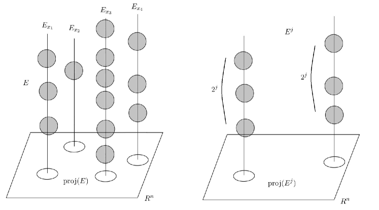
Figure 1. The sets $E$, proj$E$, $E_{x}$ and $E^{j}$ in the proof of Proposition 2.7.

By using Lemma 2.6 with

$$K:=\frac{\log(1/\epsilon)}{2\log\gamma}+1,$$

the $E^{j}$ is decomposed into $E^{j}_{k}$’s which are covered by $O(|E^{j}|^{1/K})$ number of $(O(|E^{j}|),|E^{j}|^{C\gamma^{k-1}}))$-sparse collections. We apply (2.7) to these sparse collections and obtain

$$\|\mathfrak{R}\chi_{E^{j}_{k}}\|_{L^{2}(d\sigma)}\leq C_{\epsilon}|E^{j}|^{1/K}(|E^{j}|^{C\gamma^{k-1}})^{\epsilon}\|\chi_{E^{j}_{k}}\|_{L_{x}^{q_{0}}(\mathbb{R}^{n};L_{t}^{r_{0}}(\mathbb{R}))}.$$

Summing over k, we have

$$\|\mathfrak{R}\chi_{E^{j}}\|_{L^{2}(d\sigma)} \leq\sum_{k=1}^{K}\|\mathfrak{R}\chi_{E^{j}_{k}}\|_{L^{2}(d\sigma)}$$

$$\leq C_{\epsilon}|E^{j}|^{1/K}(|E^{j}|^{C\gamma^{K-1}})^{\epsilon}\|\chi_{E^{j}}\|_{L_{x}^{q_{0}}(\mathbb{R}^{n};L_{t}^{r_{0}}(\mathbb{R}))}$$

where $K$ is absorbed into $C_{\epsilon}$. Since $|E^{j}|\leq 2^{j+1}|\mathrm{proj\,}(E^{j})|$, we have

$$\|\mathfrak{R}\chi_{E^{j}}\|_{L^{2}(d\sigma)}\leq C_{\epsilon}2^{j(\frac{1}{r_{0}}+\delta(\epsilon))}|\mathrm{proj}(E^{j})|^{\frac{1}{q_{0}}+\delta(\epsilon)},$$

where

$$\delta(\epsilon):=\frac{1}{K}+C\gamma^{K-1}\epsilon.$$

Since $\lim_{\epsilon\to 0}\delta(\epsilon)=0$, we can take $\epsilon>0$ such that

$$0<\delta(\epsilon)+\epsilon\leq\min\bigg{(}\frac{1}{q}-\frac{1}{q_{0}},\frac{1}{r}-\frac{1}{r_{0}}\bigg{)}.$$

Thus,

$$\|\mathfrak{R}\chi_{E}\|_{L^{2}(d\sigma)} \leq\sum_{j\geq 1}\|\mathfrak{R}\chi_{E^{j}}\|_{L^{2}(d\sigma)}$$

$$\leq C_{\epsilon}\sum_{j\geq 1}2^{j(\frac{1}{r_{0}}+\delta(\epsilon))}|\mathrm{proj}(E^{j})|^{\frac{1}{q_{0}}+\delta(\epsilon)}$$

$$\leq C\sum_{j\geq 1}2^{-\epsilon j}2^{\frac{1}{r}j}|\mathrm{proj}(E^{j})|^{\frac{1}{q}}$$

$$\leq C\sum_{j\geq 1}2^{-\epsilon j}\|\chi_{E}\|_{L_{x}^{q}(\mathbb{R}^{n};L_{t}^{r}(\mathbb{R}))}$$

$$\leq C\|\chi_{E}\|_{L_{x}^{q}(\mathbb{R}^{n};L_{t}^{r}(\mathbb{R}))}.$$

∎

Combining Proposition 2.5 and Proposition 2.7 we obtain an extension of Tao’s epsilon removal lemma as follows.

Proposition 2.8.

Let $1<q_{0},r_{0}\leq 2$. Suppose that

$$\|\mathfrak{R}(\chi_{\mathbb{I}_{R}\times\mathbb{B}_{R}}f)\|_{L^{2}(d\sigma)}\leq C_{\epsilon}R^{\epsilon}\|f\|_{L_{x}^{q_{0}}(\mathbb{R}^{n};L_{t}^{r_{0}}(\mathbb{R}))}$$

for all $\epsilon>0$, $R>1$ and all $f\in L_{x}^{q}(\mathbb{R}^{n};L_{t}^{r}(\mathbb{R}))$. Then for any $1\leq q<q_{0}$ and $1\leq r<r_{0}$,

$$\|\mathfrak{R}f\|_{L^{2}(d\sigma)}\leq C\|f\|_{L_{x}^{q}(\mathbb{R}^{n};L_{t}^{r}(\mathbb{R}))}$$

for all $f\in L_{x}^{q}(\mathbb{R}^{n};L_{t}^{r}(\mathbb{R}))$.

Now we are ready to prove Theorem 1.2. The theorem follows from Proposition 2.2 and Proposition 2.8 as follows.

2.3. Proof of Theorem 1.2

Let $P_{0}$ be the Littlewood-Paley projection operator as in subsection 2.1. By rescaling $x\mapsto 2^{-k}x$ and $t\mapsto 2^{-mk}t$, the estimate (1.4) implies

$$\|e^{it\Phi(D)}P_{0}f\|_{L_{x}^{q_{0}}(\mathbb{B}_{R};L_{t}^{r_{0}}(\mathbb{I}_{R^{m}}))}\leq C_{\epsilon}2^{k\epsilon}\|P_{0}f\|_{L^{2}(\mathbb{R}^{n})}$$

for all $k\geq 1$ and $\epsilon>0$. Since $m\geq 1$, we have

$$\|e^{it\Phi(D)}P_{0}f\|_{L_{x}^{q_{0}}(\mathbb{B}_{R};L_{t}^{r_{0}}(\mathbb{I}_{R}))}\leq C_{\epsilon}2^{k\epsilon}\|P_{0}f\|_{L^{2}(\mathbb{R}^{n})}.$$

By Proposition 2.8 and duality,

$$\|e^{it\Phi(D)}P_{0}f\|_{L_{x}^{q}(\mathbb{R}^{n};L_{t}^{r}(\mathbb{R}))}\leq C\|P_{0}f\|_{L^{2}(\mathbb{R}^{n})}.$$

By Proposition 2.2, we obtain the desired estimate. ∎

3. Appendix

3.1. Proof of Lemma 2.4

We divide the left side of (2.4) into two parts

$$\|\sum_{i=1}^{N}f_{i}\ast\hat{\varphi}_{i}|_{S}\|_{2}^{2}=\sum_{i}\|f_{i}\ast\hat{\varphi}_{i}|_{S}\|_{2}^{2}+\sum_{i\neq j}\int f_{i}\ast\hat{\varphi}_{i}\overline{f_{j}\ast\hat{\varphi}_{j}}d\sigma.$$

By a basic restriction estimate we have $\|f_{i}\ast\hat{\varphi}_{i}|_{S}\|_{2}\lesssim R^{1/2}\|f_{i}\|_{2}$. Thus,

$$\sum_{i=1}^{N}\|f_{i}\ast\hat{\varphi}_{i}|_{S}\|_{2}^{2}\lesssim R\sum_{i=1}^{N}\|f_{i}\|_{2}^{2}.$$ (3.1)

By Parseval’s identity,

$$\int f_{i}\ast\hat{\varphi}_{i}\overline{f_{j}\ast\hat{\varphi}_{j}}d\sigma=\int\overline{\check{f}_{j}\varphi_{j}}((\check{f}_{i}\varphi_{i})\ast\widehat{d\sigma}),$$

where the $\check{}$ denotes the inverse Fourier transform. It is bounded by

$$\big{(}\sup_{z,w}|\varphi_{j}^{1/2}(z)\varphi^{1/2}_{i}(w)\widehat{d\sigma}(z-w)|\big{)}\|\check{f}_{i}\varphi^{1/2}_{i}\|_{1}\|\check{f}_{j}\varphi^{1/2}_{j}\|_{1}.$$

By the Cauchy-Schwarz inequality and Plancherel’s theorem,

$$\|\check{f}_{i}\varphi^{1/2}_{i}\|_{1}\lesssim R^{(n+1)/2}\|f_{i}\|_{2}.$$

By (2.3),

$$\sup_{z,w}|\varphi^{1/2}_{j}(z)\varphi^{1/2}_{i}(w)\widehat{d\sigma}(z-w)|\lesssim|z_{i}-z_{j}-2R|^{-\rho}.$$

Since $|z_{i}-z_{j}|\geq(NR)^{\gamma}$ and $\gamma\geq 2$, we have that $|z_{i}-z_{j}-2R|$ is comparable to $|z_{i}-z_{j}|$. Thus,

$$\sup_{z,w}|\varphi^{1/2}_{j}(z)\varphi^{1/2}_{i}(w)\widehat{d\sigma}(z-w)|\lesssim|z_{i}-z_{j}|^{-\rho}.$$

Combining these estimates we have

$$\sum_{i\neq j}\int f_{i}\ast\hat{\varphi}_{i}\overline{f_{j}\ast\hat{\varphi}_{j}}d\sigma \lesssim R^{n+1}\sum_{i=1}^{N}\sum_{j=1}^{N}|z_{i}-z_{j}|^{-\rho}\|f_{i}\|_{2}\|f_{j}\|_{2}$$

$$\lesssim R^{n+1}N\max_{i,j}|z_{i}-z_{j}|^{-\rho}\sum_{i=1}^{N}\|f_{i}\|_{2}^{2}.$$

Since $|z_{i}-z_{j}|\geq(NR)^{\gamma}\geq N^{\frac{1}{\rho}}R^{\frac{n}{\rho}}$, it follows that

$$\sum_{i\neq j}\int f_{i}\ast\hat{\varphi}_{i}\overline{f_{j}\ast\hat{\varphi}_{j}}d\sigma\lesssim R\sum_{i=1}^{N}\|f_{i}\|_{2}^{2}.$$

From the above estimate and (3.1) we obtain (2.4). ∎

3.2. Proof of Lemma 2.6

Fix $K\in\mathbb{N}$. We define $R_{0}=1$ and $R_{k}$ for $k=1,2,\cdots,K$ recursively by

$$R_{k}=|E|^{\gamma}R_{k-1}^{\gamma}.$$ (3.2)

From this definition we have $R_{k}=|E|^{\frac{\gamma^{k+1}-\gamma}{\gamma-1}}$. Let $E_{0}=\emptyset$. We define $E_{k}$ for $k=1,2,\cdots,K$ to be the set of all $x\in E\setminus\cup_{j=0,1,2,\cdots,k-1}E_{j}$ such that

$$|E\cap B(x,R_{k})|\leq|E|^{k/K}.$$ (3.3)

Then, $E=\bigcup_{k=1}^{K}E_{k}$. From this construction it follows that that for $x\in E_{k}$, $k=2,3,\cdots,K$,

$$|E\cap B(x,R_{k-1})|>|E|^{(k-1)/K}.$$ (3.4)

We cover $E_{k}$ with finitely overlapping $R_{k}$-balls $\mathbf{C}_{E_{k}}:=\{B_{i}=B(x_{i},R_{k}):x_{i}\in E_{k}\}$. Since $E$ is a finite union of cubes of side-length $c\sim 1$, it is obvious that $\#\mathbf{C}_{E_{k}}\lesssim|E|$. For each $B_{i}\in\mathbf{C}_{E_{k}}$ we cover $E_{k}\cap B_{i}$ with finitely overlapping $R_{k-1}$-balls $\mathbf{C}_{E_{k}\cap B_{i}}:=\{B^{\prime}_{ij}=B^{\prime}(y_{j},R_{k-1}):y_{j}\in E_{k}\cap B_{i}\}$, that is,

$$E_{k}\cap B_{i}=\bigcup_{B^{\prime}_{ij}\in\mathbf{C}_{E_{k}\cap B_{i}}}E_{k}\cap B_{ij}^{\prime}.$$

Since $((E\setminus E_{k})\cap B_{ij}^{\prime})\subset((E\setminus E_{k})\cap B_{i})$ for all $j$, we have

$$(E_{k}\cap B_{i})\cup((E\setminus E_{k})\cap B_{i})\supset\bigcup_{B^{\prime}_{ij}\in\mathbf{C}_{E_{k}\cap B_{i}}}(E_{k}\cap B_{ij}^{\prime})\cup((E\setminus E_{k})\cap B_{ij}^{\prime}),$$

thus

$$E\cap B_{i}\supset\bigcup_{B^{\prime}_{ij}\in\mathbf{C}_{E_{k}\cap B_{i}}}E\cap B_{ij}^{\prime}.$$

By finitely overlapping,

$$\#\mathbf{C}_{E_{k}\cap B_{i}}\lesssim\max_{B^{\prime}_{ij}\in\mathbf{C}_{E_{k}\cap B_{i}}}\frac{|E\cap B_{i}|}{|E\cap B_{ij}^{\prime}|}.$$

By (3.3) and (3.4) the above is bounded by $C|E|^{1/K}$, and we have $\#\mathbf{C}_{E_{k}\cap B_{i}}\leq C|E|^{1/K}$ for all $i$. Thus,

$$E_{k}\subset\bigcup_{i=1}^{O(|E|)}\bigcup_{j=1}^{O(|E|^{1/K})}B_{ij}^{\prime}.$$

We choose $O(R_{k})$-separated balls $\{B^{\prime}_{ij(i)}\}_{i=1}^{O(|E|)}$. Then it becomes a $(O(|E|),R_{k-1})$-sparse collection because of (3.2). Since $R_{k-1}=|E|^{O(\gamma^{k-1})}$ and every $B_{i}\in\mathbf{C}_{E_{k}}$ has the covering $\mathbf{C}_{E_{k}\cap B_{i}}$ of cardinality $O(|E|^{1/K})$, there are $O(|E|^{1/K})$ number of $(O(|E|),|E|^{O(\gamma^{k-1})})$-sparse collections $\mathbf{S}_{1},\mathbf{S}_{2},\cdots,\mathbf{S}_{O(|E|^{1/K})}$ such that

$$E_{k}\subset\bigcup_{j=1}^{O(|E|^{1/K})}\bigcup_{B^{\prime}\in\mathbf{S}_{j}}B^{\prime}.$$

∎