QUASI-NEWTON METHODS FOR MINIMIZING A QUADRATIC FUNCTION SUBJECT TO UNCERTAINTY
Abstract
We investigate quasi-Newton methods for minimizing a strictly convex quadratic function which is subject to errors in the evaluation of the gradients. The methods all give identical behavior in exact arithmetic, generating minimizers of Krylov subspaces of increasing dimensions, thereby having finite termination. A BFGS quasi-Newton method is empirically known to behave very well on a quadratic problem subject to small errors. We also investigate large-error scenarios, in which the expected behavior is not so clear. In particular, we are interested in the behavior of quasi-Newton matrices that differ from the identity by a low-rank matrix, such as a memoryless BFGS method. Our numerical results indicate that for large errors, a memory-less quasi-Newton method often outperforms a BFGS method. We also consider a more advanced model for generating search directions, based on solving a chance-constrained optimization problem. Our results indicate that such a model often gives a slight advantage in final accuracy, although the computational cost is significantly higher.
Keywords: Quadratic programming, quasi-Newton method, stochastic quasi-Newton method, chance constrained model
1 Introduction
A strictly convex -dimensional quadratic function may be written on the form
where is a positive definite and symmetric -matrix, is an -dimensional vector and is a constant. The optimization problem of minimizing is equivalent to solving , i.e., solving the linear equation .
One way to do so by a direct method is to find an initial point and associated gradient . Then generate and , with , such that is the minimizer of on , where
This is equivalent to being orthogonal to , so that , , …, form an orthogonal basis for . Since there can be at most nonzero orthogonal vectors, there is an , with , such that . Consequently, is the minimizer of .
A method for computing , , …, this way is characterized by the search direction leading from to . Given , the step length is given by minimizing , i.e.,
| (1.1) |
Therefore, it suffices to characterize . One characterization is given by the conditions that
| is a linear combination of , , , , in addition to | (1.2a) | ||||
| satisfying , | (1.2b) | ||||
see, e.g., [EF21, Lemma 1]. There could be an arbitrary scaling for a nonzero scalar . Throughout, we will use .
The method of conjugate gradients gives a short recursion for the search direction satisfying (1.2). It may be written on the form
| (1.3) |
See, e.g., [Saa03, Chapter 6] for an introduction to the method of conjugate gradients.
An alternative way of computing the search direction satisfying (1.2) is through a quasi-Newton method, in which is defined by a linear equation , for a symmetric positive-definite matrix. A well-known method for which gives satisfying (1.2) is the BFGS quasi-Newton method, in which , and is formed by adding a symmetric rank-2 matrix to . In our setting, the BFGS method may be viewed as the “ideal” update that dynamically transforms from to in steps. Identity curvature is transformed to curvature in one dimension at each step, and this information is maintained throughout. The precise formulas will be given in Section 2.
In exact arithmetic, the method of conjugate gradients and a BFGS quasi-Newton method compute identical iterates in the setting we consider, minimizing a strictly convex quadratic problem using exact linesearch. In this situation, the recursion formula for the method of conjugate gradients is to prefer, since the computational cost for solving with for the BFGS method increases with .
In finite precision arithmetic, the BFGS quasi-Newton method may still be expected to compute search directions of very high quality as the Hessian is approximated on subspaces of higher dimension. This is not to be expected for the method of conjugate gradients. Our interest is to study the situation where noise is added to the gradients, thereby considering a situation with significantly higher level of error than finite precision arithmetic. In this situation, it is not clear that the BFGS quasi-Newton method is superior, in the sense that the Hessian approximation may become inaccurate. It is here also of interest to consider the method of steepest descent, where the search direction is the negative of the gradient. For exact arithmetic, the search directions satisfying (1.2) will outperform steepest descent due to the property of minimizing the quadratic objective function over expanding subspaces. In the case of large noise, this is not at all clear.
The reason for noise in the gradients can be seen in different perspectives. Firstly, as mentioned above, the finite precision arithmetic gives a residual between the evaluated gradients and the true gradients. Secondly, in many practical problem, such as PDE-constrained optimization, the objective function often contains computational noise created by an inexact linear system solver, adaptive grids, or other internal computations. In other cases, the noise in the gradients can be due to stochastic errors. For example, when minimizing , where is a random variable. With given sample set , instead of , the following empirical expectation will be considered:
Due to the randomness of samples, , and , where are random noise.
The basis for the methods we consider is that they compute search directions identical to those of the BFGS method and the method of conjugate gradients, i.e., satisfying (1.2), in exact arithmetic. In particular, we are interested in a setting where is the identity matrix plus a symmetric matrix of rank two. We will refer to such a quasi-Newton matrix as a low-rank quasi-Newton matrix and name the corresponding method a low-rank quasi-Newton method. Our intention is to investigate the behavior of a low-rank quasi-Newton method compared to the method of steepest descent, thereby mimicking a situation where two more vectors in addition to are used at iteration . The corresponding search direction can then be computed from a two-by-two system. For comparison, we also compare to the BFGS quasi-Newton method. Our choice of quadratic problem allows an environment where the behavior of the methods in infinite precision is known, and we can study the effect of noise.
In addition, we investigate the potential for improving performance of the quasi-Newton method by formulating robust optimization problems of chance-constraint type for computing the search directions. These methods become of higher interest in the case of large noise and multiple copies of the gradients. Our interest is to capture the essence of the behavior, and try to understand the interplay between quality in computed direction compared to robustness given by the chance constraints. The computational cost will always be significantly higher, but our interest is to see if we can gain in terms of robustness and accuracy of the computed solution.
1.1 Background and related work
The paper builds on previous work in the setting of exact arithmetic and finite precision arithmetic. Forsgren and Odland [FO18] have studied exact linesearch quasi-Newton methods for minimizing a strictly convex quadratic function, and given necessary and sufficient conditions for a quasi-Newton matrix to generate a search direction which is parallel to that of (1.2) in exact arithmetic. With exact linesearch methods, Ek and Forsgren [EF21] have studied certain limited-memory quasi-Newton Hessian approximations for minimizing a convex quadratic function in the setting of finite precision arithmetic. Dennis and Walker [DW84] have considered the use of bounded-deterioration quasi-Newton methods implemented in floating-point arithmetic where only inaccurate values are available. In contrast, our work allows for large noise and we study performance on a set of test problems.
In the present manuscript, we consider a situation where the function values and gradients cannot be easily obtained and only noisy information about the gradient is available. To handle this situation, some stochastic methods are proposed to minimize the objective function with inaccurate information. Our setting is minimizing a strictly convex quadratic function.
For strongly convex problems, Mokhtari and Ribeiro [MR13] have proposed a regularized stochastic BFGS method and analyzed its convergence, and Mokhtari and Ribeiro [MR15] have further studied an online L-BFGS method. Berahas, Nocedal and Takac [BNT16] have considered the stable performance of quasi-Newton updating in the multi-batch setting, illustrated the behavior of the algorithm and studied its convergence properties for both the convex and nonconvex cases. Byrd et al. [BHNS16] have proposed a stochastic quasi-Newton method in limited memory form through subsampled Hessian-vector products. Shi et al. [SXBN20] have proposed practical extensions of the BFGS and L-BFGS methods for nonlinear optimization that are capable of dealing with noise by employing a new linesearch technique. More recently, Xie, Byrd and Nocedal [XBN20] have considered the convergence analysis of quasi-Newton methods when there are (bounded) errors in both function and gradient evaluations, and established conditions under which an Armijo-Wolfe linesearch on the noisy function yields sufficient decrease in the true objective function.
Unlike the stochastic quasi-Newton methods, which are based on the subsampled gradients or Hessians, there are also other stochastic tools to reduce the effect of noise when generating the search direction. Lucchi et al. [LMH15] have studied quasi-Newton method by incorporating variance reduction technique to reduce the effect of noise in Hessian matrices by proposing a variance-reduced stochastic Newton method. This method keeps the variance under control in the use of a multi-stage scheme. Moritz et al. [MNJ16] have proposed a linearly convergent method that integrates the L-BFGS method to alleviate the effect of noisy gradients with the variance reduction technique by adding the residual between subsample gradient and full gradient to the noisy gradient.
In addition, chance constraint is a natural approach to handle the effect of random noise [AX18]. Therefore, chance constraint has the potential to reduce the effect of noise when generating the search direction. By integrating chance constraints in the design of quasi-Newton methods, we investigate the ability to improve robustness into the computation of the search direction in the presence of noise.
2 Suggestions on quasi-Newton matrices
As mentioned in Section 1, a well-known method for which gives satisfying (1.2) is the BFGS quasi-Newton method. In the BFGS method, and
| (2.1) |
Expansion gives
| (2.2) |
For the quadratic case with exact linesearch, the BFGS matrix of (2.2) takes the form
| (2.3) |
see, e.g., [EF21]. If steps are taken, then with , it follows that is square and nonsingular, so that
| (2.4) |
where the conjugacy of the s is a consequence of (1.2). In this situation, (2.3) may therefore be seen as a dynamic way of generating the true Hessian in steps, if the method does not converge early, as by
This is a consequence of the orthogonal gradients then spanning the whole space in combination with (2.4). Consequently, the BFGS method may be viewed as the “ideal” update that dynamically transforms from to in steps. Identity curvature is transformed to curvature in one dimension at each step, and this curvature information is maintained throughout.
The discussion above may be generalized to a general class of quasi-Newton matrices of the form
| (2.5) |
where for satisfying (1.2), and , , are nonnegative scalars. In exact arithmetic and under exact linesearch, the specific values of , , have no impact on the search direction, due to (1.2). In a noisy framework, they will make a difference, and we will pay attention to how they are selected.
As discussed in Section 1, we are particularly interested in low-rank quasi-Newton matrices. We will therefore consider a memoryless BFGS quasi-Newton method, in which
| (2.6) |
in addition to , , so that
| (2.7) |
where the value of is given by the secant condition . We denote this particular value of by . For exact linesearch, of (2.7) gives
| (2.8) |
Then for satisfying (1.2) in the case of exact arithmetic, see, e.g., [FO18, Proposition 1]. The of the memoryless BFGS matrix given by (2.6) is analogous to the first two terms of the BFGS matrix of (2.3), but the matrix is singular with its nullspace restricted to the one-dimensional span of , as opposed to the span of all previous gradients. In addition, the memoryless BFGS matrix of (2.7) is nonsingular as and .
We will also interpret the method of conjugate gradients in a quasi-Newton framework, by forming the symmetric CG quasi-Newton matrix given by
| (2.9) |
This matrix is formed by rewriting the recursion (1.3) and making an additional symmetrization, see [FO18]. It can be put in the matrix family given by (2.5) by setting and , .
In summary, we will consider quasi-Newton matrices of the form (2.5). In particular, we will consider two specific low-rank matrices. The quasi-Newton matrices given by memoryless BFGS in (2.7) and symmetric CG in (2.9) are both low-rank quasi-Newton matrices that differ from the identity by a symmetric rank two matrix and fulfill the conditions we require, (1.2). They will be used in our computational study.
3 A chance-constrained model for finding the search direction
In addition to investigating the behavior of the quasi-Newton methods discussed so far, we are also interested in investigating the potential of increasing the performance of the quasi-Newton methods in the presence of noise by selecting parameters from a chance-constrained optimization problem.
The aim is to design a quasi-Newton matrix , with , so as to compute a search direction of high quality. For the case of exact arithmetic, i.e., no noise, our model direction is the direction that satisfies (1.2). The interest is now to investigate and design quasi-Newton matrices in the presence of noise. In particular, we are interested in studying the performance of different methods for different noise levels. For a given quasi-Newton matrix , the search direction is computed from .
As there exists noise in each iteration, it means that the obtained gradient is not accurate, it is the combination of the true gradient and some white noise. The update of search direction may result in a non-descent direction because of the influence by the noise. Then, we have the following proposition to show that the search direction satisfying is a descent direction under certain conditions even with noise in each iteration.
Proposition 3.1
Consider iteration of a quasi-Newton method for minimizing . Let , where is the true gradient and is the noise generated with mean equal to . If and , the direction , satisfying , is a descent direction at point .
Proof. The direction is a descent direction if . Since , we have
Hence, is a descent direction if .
As , implies is a descent direction. This concludes the proof.
A consequence is that the property of being a descent direction may be lost if the termination criteria on is set smaller than the noise level, as observed in the following remark.
Remark 1
Proposition 3.1 shows that when the noise is small enough, the direction satisfying is a descent direction. However, if the noise is large, the direction obtained from may not be a descent direction. In particular, let denote the tolerance level of the stopping criterion based on . Consider the situation when . If is close to termination solution, the value of is close to . In this case, we could have . Since , the conditions in Proposition 3.1 can not hold. Therefore, the direction satisfying may be not a descent direction anymore.
In our quasi-Newton setting, the aim is not only to generate descent directions, but also to generate search directions of high quality. Suppose is a quality measure for the search direction at iteration . The aim is to minimize the quality measure such that . Therefore, for a given quality measure , we can generate a search direction with highest quality by solving the following optimization problem:
| (3.1) |
In addition, we typically require to have some additional properties, as problem (3.1) becomes highly complex otherwise.
The model (3.1) is actually a deterministic model, where the noisy gradients are deterministic. However, as mentioned in Section 1, in some practical problems, the gradients themselves are random because of the randomness in the original objective quadratic function. Therefore, it is more natural to view the gradients as random vectors in model (3.1). At iteration , it is assumed that , where is a random noise with mean equal to . Hence, considering the randomness and to overcome the shortcoming of model (3.1) as mentioned in Remark 1, the model (3.1) can be formulated as the following chance constrained model:
| (3.2) |
where is a given probability level. The value of indicates the risk-aversion of the decision maker, where 0 is the most conservative approach as we need to comply with the supremum value of the underlying random vector, while higher values would make our solution averse to risk. Even small values of can have significant impact to the results [BHdMM+16], therefore studying the behaviour of the solution while is 0 and close to 0 (typically 0.01 or 0.05) is the usual approach. The chance constraint in problem (3.2) not only guarantees the validation of quasi-Newton setting with probability at least , but also controls the quality measure of the search direction.
To show that the search direction obtained by solving problem (3.2) is a descent direction with a high probability, we have the following proposition.
Proposition 3.2
Denote , where is the true gradient and is a random noise with mean equal to . If is invertible and , the direction satisfying the chance constraint in problem (3.2) is a descent direction at point with probability at least .
Proof. From Proposition 3.1, we have that the direction is a descent direction if the following constraints are satisfied:
Then, we have
The second inequality comes from Fréchet inequality. Therefore, the conclusion can be obtained.
In contrast to the deterministic case, we can still maintain a descent direction with positive probability even for , as observed in the following remark.
Remark 2
A chance-constrained model is expected to be computationally expensive. Our interest is to study its behavior, in particular to see how such an approach might be able to achieve improved accuracy, as indicated by Remark 2.
3.1 Suggestion on quality measure
With these propositions concerning the search direction, an interesting issue is how to determine the quality measure of the search direction when the method is applied to an unconstrained quadratic optimization problem. We suggest an approach based on the characterization given in (1.2). In the exact arithmetic case, (1.2) gives , . Therefore, in this situation, the desired would give a global minimum zero with respect to the measure
| (3.5) |
In the exact arithmetic case, is orthogonal to the affine span of the generated gradients. In the noisy setting, we will use this measure to show how close the direction is to the characterization in (1.2).
Motivated by the discussion above, at iteration , for a given positive semidefinite matrix , we will consider quasi-Newton matrices in the family given by (2.5) and wish to find as the solution of
| (D) |
For the given , in exact arithmetic and under exact linesearch, the specific values of have no impact on the search direction. However, the specific values may ensure nonsingularity of and numerical stability. Note also that the sum of rank-one matrices in (2.5) is similar to terms present in the BFGS Hessian approximation of (2.2).
Considering the possible randomness in the gradient , the chance constrained model (3.2) should take equations (2.5) and (3.5) into consideration. In addition, from (2.9), we can notice that the matrix can be dependent on the noisy gradient in some cases, which implies that is random. Therefore, in the random case, we denote
| (3.6) |
where is a random matrix. Assume that the gradients , have been evaluated, which can be the realized values of noisy gradients or average values of noisy gradient samples. Then, based on model (D), the chance constrained model for finding the search direction, associated with model (3.2), can be formulated as
| (C) |
In model (C), only is the random vector, while , are constant values.
4 Reformulation for the low-rank quasi-Newton setting
Models (D) and (C) are hard to solve given the non-convex nature of the equality-constraints created by the condition and the associated condition on , and the nature of the chance constraints. In the low-rank setting, however, the constraints related to the quasi-Newton matrix can be simplified significantly.
In our low-rank setting, the only unknown parameter is for the memoryless BFGS matrix, where we may write
and treat as a variable. For this case, we may allow further simplification by circumventing the possible singularity of by letting be the value given by the secant condition (2.8), and writing
| (4.1) |
for
| (4.2) |
For the memoryless BFGS matrix, it holds that is positive semidefinite with at most one zero eigenvalue in addition to , so that as . The point of introducing and is to give a nonsingular and positive definite , which may be used as a foundation for optimizing over . We may therefore view the optimization over as the potential for improving over utilizing the secant condition.
For a such that in (4.1), the Sherman-Morrison formula gives
| (4.3) |
for
| (4.4) |
so that an explicit expression for may be given as
Note that there is a one-to-one correspondence between and as (4.4) gives
| (4.5) |
In addition, if , then (4.4) and (4.5) show that if and only if the equivalent conditions
hold. This is a consequence of these lower bounds defining an interval around and respectively, where and are well defined.
Summarizing, we may formulate the simplified problem as
| (DS) |
which is a convex constrained quadratic program if a tolerance is introduced for the strict lower bound on . For this problem, we may eliminate to get one variable only, . Note the one-to-one correspondence given by (4.5) which allows us to recover from .
For the chance-constrained model (C), analogous to (3.6), we denote
| (4.6) |
for
| (4.7) |
which is random due to the randomness of . is deterministic as defined in (2.6). Then, analogous simplification and reformulation of (C) gives
| (CS) |
Our proposed model (CS) can be read as follows: the obtained solution , which will be transformed to by (4.5), will have a probability of at least to obtain a direction from that will be a descent direction. This means our approach obtains a value of robust enough to point us in a descent direction with a probability bounded given the probabilistic nature of the gradient.
Chance constrained models are often non-convex in general and hard to solve [SDR14]. However, different equivalent formulations can be applied to obtain an analytical solution or approximate the chance constraints. In general, it is often difficult to get an analytical solution, since it always requires strict assumptions on the probability distribution of random variables and the structure of chance constraints, which making the situation specific and not general enough. In constrast to the analytical solution, sample average approximation and scenario approximation are two general approaches without much assumptions on the random variables, which will be applied to solve the chance constrained model in the following sections.
4.1 Deterministic equivalent formulation
Model (CS) can not be solved directly in its current state, as it is not a deterministic problem. Therefore, a sample average approximation (SAA) approach is proposed, given its flexibility to work under any type of stochastic variables. The first step is to formulate it as a deterministic problem that approximates the solution of (CS) and that can be solved by some solvers. Let be the set of sample, , be the i.i.d. noisy gradient samples, a sufficiently small real number and be an integer number that represent the time window to be considered in the model. All samples have a probability of . Then, a deterministic equivalent formulation of (CS) using sample average approximation (SAA) is as follows:
| (CSA) |
where and indicates the number of gradients to be considered in the model. Once we obtain the optimal value of , then is approximated by
| (4.8) |
where and is obtained by replacing in (4.7) with . Finally, is obtained using the equation
| (4.9) |
i.e., using the average of the gradients at iteration .
It can be noticed that if then (CSA) is a mixed integer program whose complexity will be tied to the number of dimensions and samples used to solve the problem. Since at every iteration new gradients are added, the dimensionality of the problem will grow at each step regardless. And to guarantee the quality of solution by SAA, the sample size should not be too small if the dimension is large.
Therefore the complexity of this approach grows at each step, leading to increasing solving times which will be an issue on long runs with low convergence speed. However, by using the value of parameter with values greater than 0, we can use a limited memory or memoryless, implementation to avoid this.
If , then all binary variables must be set to zero and can be eliminated from the problem, creating a continuous linear program which is much simpler to solve. This is commonly referred to the scenario approach, where all possible sampled scenarios of the random variables are being considered. This also implies that the solution will be closely tied to the most conservative of the sampled scenarios. There are other approaches to simplify and approximate this model present in the literature [AX18].
5 Computational results for the quasi-Newton methods
Two sets of results are presented: First, we consider a set of randomly generated problems intended to illustrate the properties and methodologies proposed in this paper. The second set of problems are real-life instances from the CUTEst test set [GOT15], to test the applicability of these methods in a more realistic environment.
A comparison of the results is provided using different models and/or approximation formulations, and we discuss the practical implications obtained with each method. All models are implemented in Python 3.7.10, using Gurobi 9.1 as a solver for the resulting optimization problems and all computation were done on an Intel(R) i7 @ 2.7 GHz and 16 GB of memory over macOS 10.
The methods chosen in our experiments are as follows:
-
•
Steepest Descent (SD):
-
•
Conjugate Gradients (CG): The symmetric CG method as presented in (2.9),
- •
- •
- •
-
•
Limited Memory Chance-Constrained Quasi Newton (lm-CCQN ). Same as CCQN, but .
In order to standardize our results across different experiments, performance profiles are used in two different analyses: First, for the number of steps required by the method to break a certain gradient norm value which will define as the tolerance level (denoted as ), then by taking the method with the lowest possible value of steps as the comparison point, we show how much larger the values of the other methods are compared to this minimum. Next, a performance profile is created to detect the minimum value of the gradient norm. Finally, the total amount of times the different experiments using a set method were able to reach a set thresholds is summed and presented: Starting from 1 (being the minimum) up to 20 (i.e. 20 times the value of the minimum). This methodology is fully expanded in [EF21].
Since noise will severely distort the gradient norms once it reaches a certain point in the run, a set of performance profiles are created for tolerance values close to the noise variance, i.e. if the variance then these performance profiles will be set to tolerances such as and . Higher does not show significant differences to the deterministic case, and lower can cause the method to not reach any threshold.
For every experiment, we applied the following algorithm: At iteration , denotes our tolerance threshold of precision for the norm of the gradient of the solution obtained, is the average value of the gradient , denotes the number of gradients to be used in the calculations and is the maximum number of steps. When calculating the step length , an exact line search approach is used with the value of the gradient without noise (the deterministic value of ), as the objective is to isolate the effects of each method in finding a descent direction. The algorithm goes as follows:
All experiments are repeated 30 times using different random number generator seeds and using 20 samples of noisy gradients at each step, therefore the performance profiles also separate each method and experiment by seed. We used a maximum amount of steps and for the lm-CCQN method.
5.1 Results for randomly created problems
The first experiment is a set of randomly generated unconstrained quadratic problems. For each problem, the Hessian matrix is defined as , where , , is the unit matrix, is a matrix, each component of is randomly generated following a Uniform(0,1) distribution and is a sufficiently small number. The vector is randomly generated as . In our experiments, we defined and .
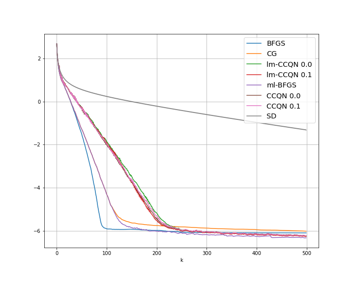
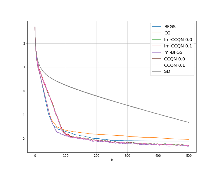
Figure 1 shows the behaviour of each method in the two selected noise levels. The traditional approaches, such as CG or BFGS, appear to converge faster but the average log norm of the gradient can not surpass the tolerance threshold smaller than the noise variance , while for CCQN and lm-CCQN (regardless of the value ) the average log norm of the gradient can surpass this barrier, albeit slower compared to the results presented by ml-BFGS.
In this experiment, the chosen value of was not large enough for SD to show convergence as seen in figure 1, however we ran the same experiment for this method using a larger value, showing that average log norm of the gradient found by SD can suprass the barrier, similar to CCQN, lm-CCQN and ml-BFGS.
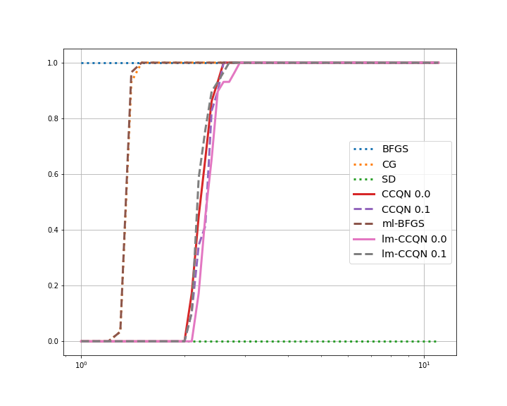
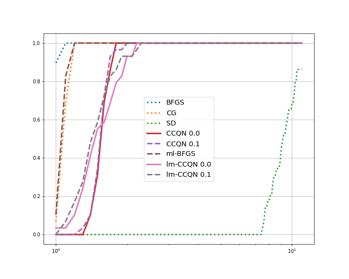
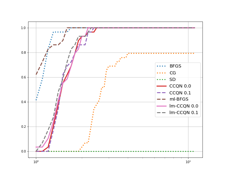
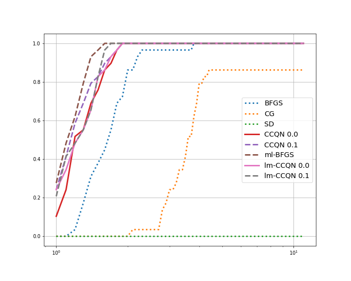
Figure 2 shows the performance profiles of each method for two noise variance levels under two tolerance thresholds. In the traditional approaches, we can observe that ml-BFGS performs better overall, while CG and BFGS perform well under low noise variance but poorly under larger values. On the other hand, the performance of CCQN and lm-CCQN methods do not show significant differences for different tolerance and noise variance levels. Furthermore, the difference between using or 0 is not significant, which means we implement a convex approximation using the scenario approach (), avoiding the usage of a mixed integer linear program which becomes difficult to solve for larger problems.
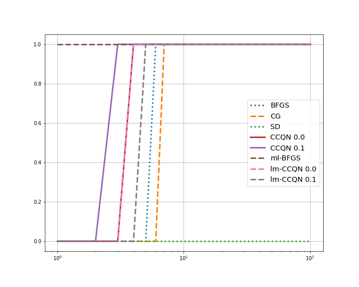
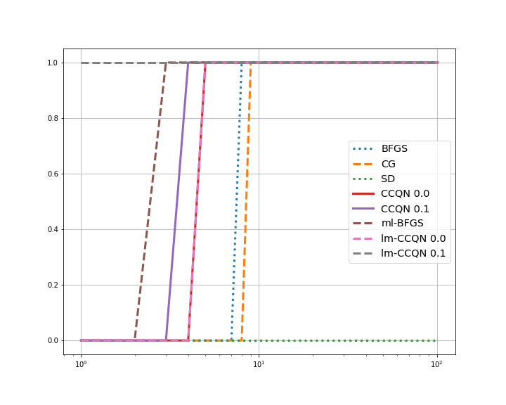
Figure 3 shows the performance profiles of the minimum gradient norm found in the set of problems with different seeds for two noise variance levels. When , we can observe that ml-BFGS is able to obtain the minimum value consistently, i.e. for every problem and every seed, which is followed by CCQN and lm-CCQN. When , lm-CCQN performs better than ml-BFGS, and followed by CCQN. The classical methods BFGS, CG and SD perform worse than the previously discussed methods independent of the noise variance, and specifically the minimum gradient norms found by SD are larger than any of minimum norms found by all the other methods.
5.2 Results for CUTEst problems
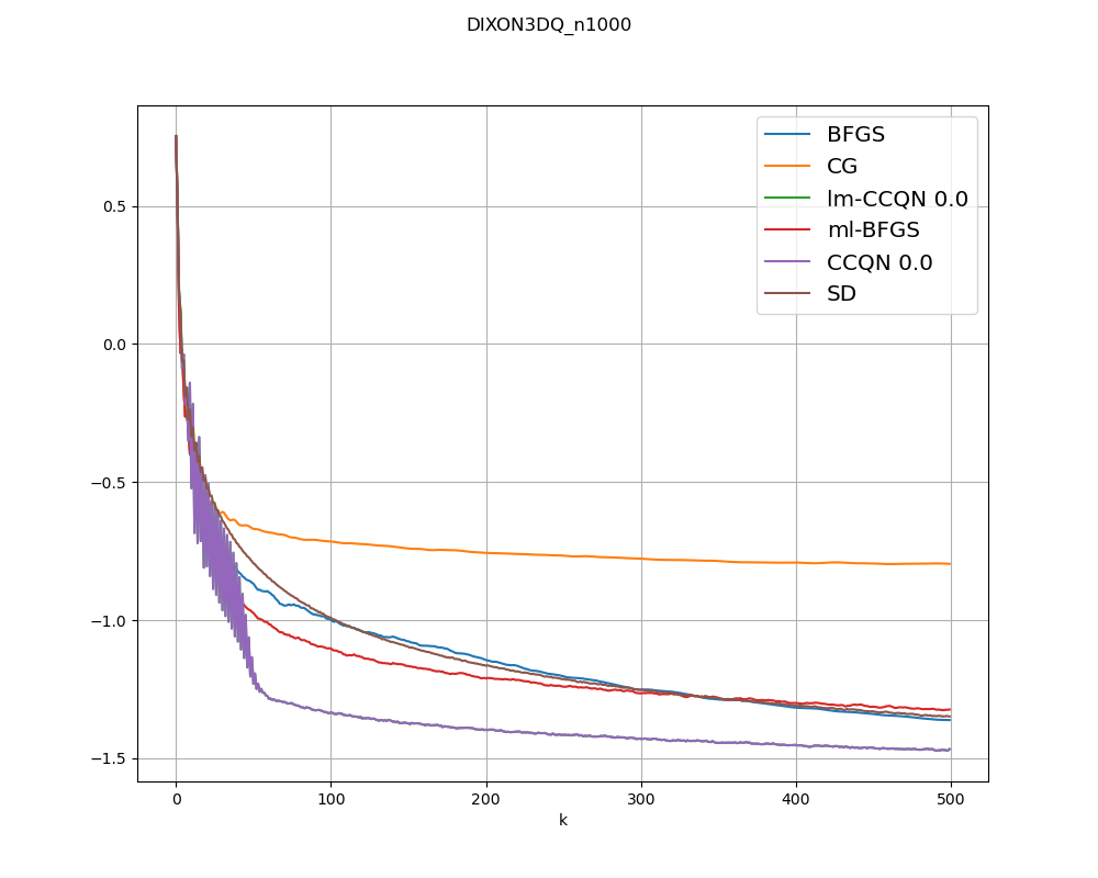
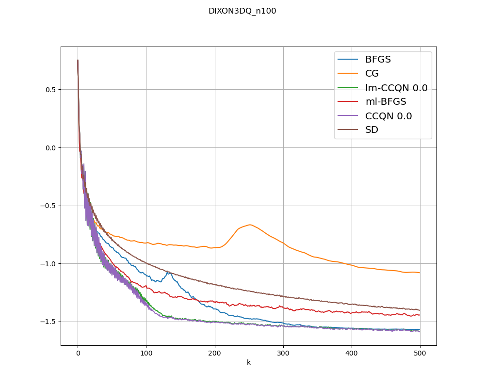
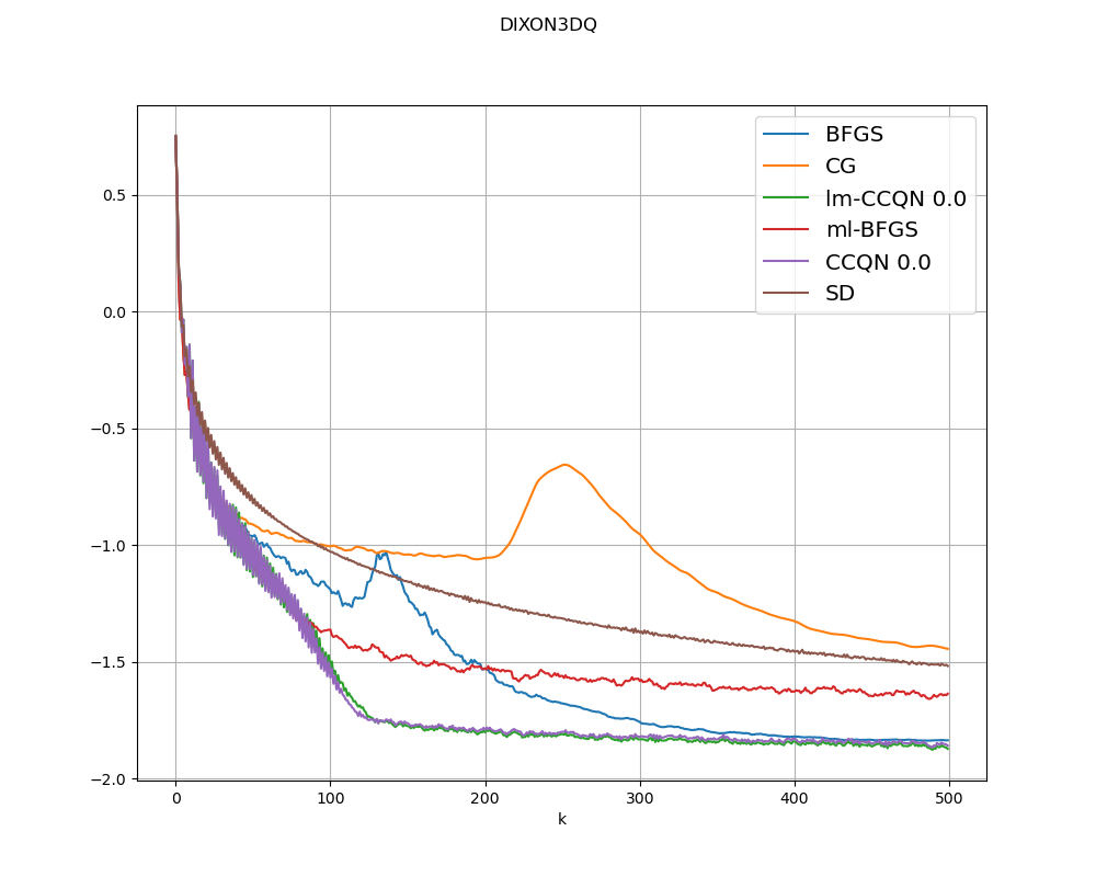
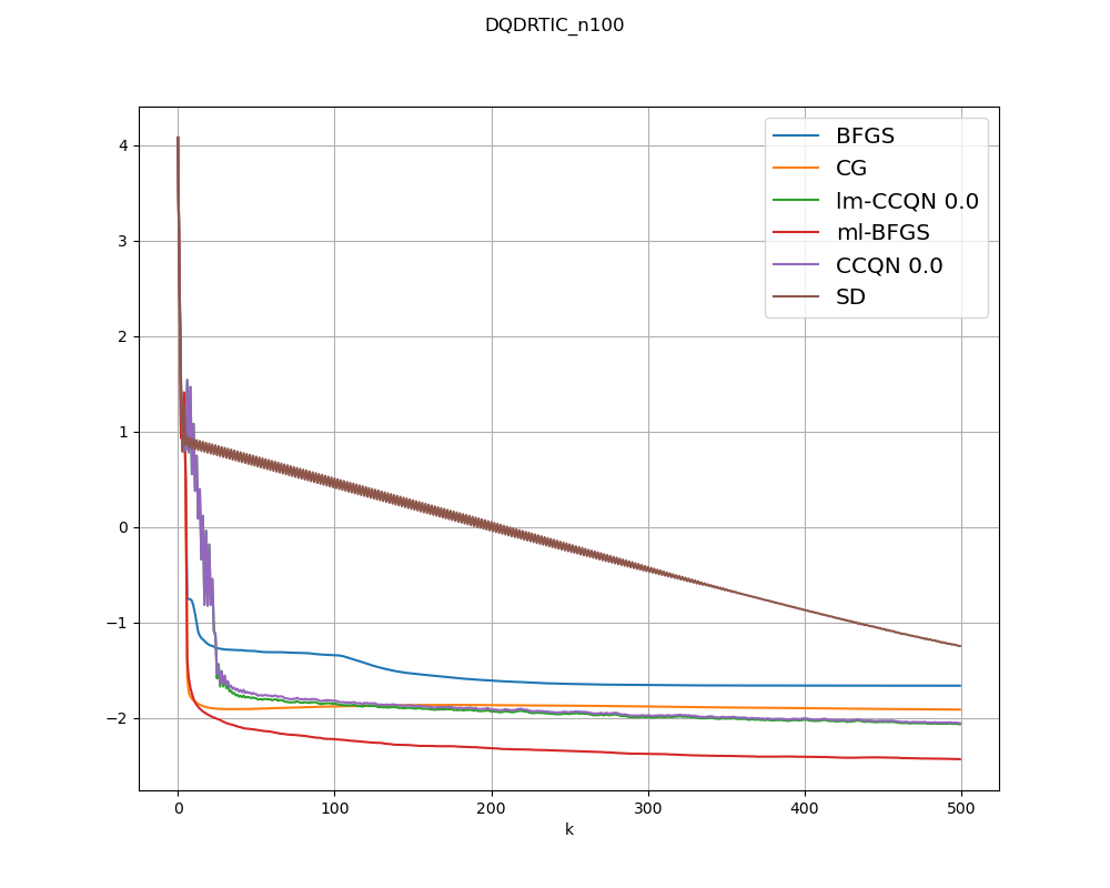
In our experiments, we will compare the performance of the same approaches presented in the last section applied to different problems from the CUTEst test set [GOT15], specifically quadratic, unconstrained and number of variables chosen by the user (QUV using CUTEst classification system). However, only 6 problems families fall in this category, therefore we implemented a second batch of problems by adding those unconstrained sum of squares problems (SUV using CUTEst classification system) which had a positive definite Hessian at the starting point and left it constant throughout the solving scheme. This brought the total amount of problems to 22. In our numerical experiments, results for noise variance and did not show significant differences. Therefore, in this section we only focus on results with a noise variance of .
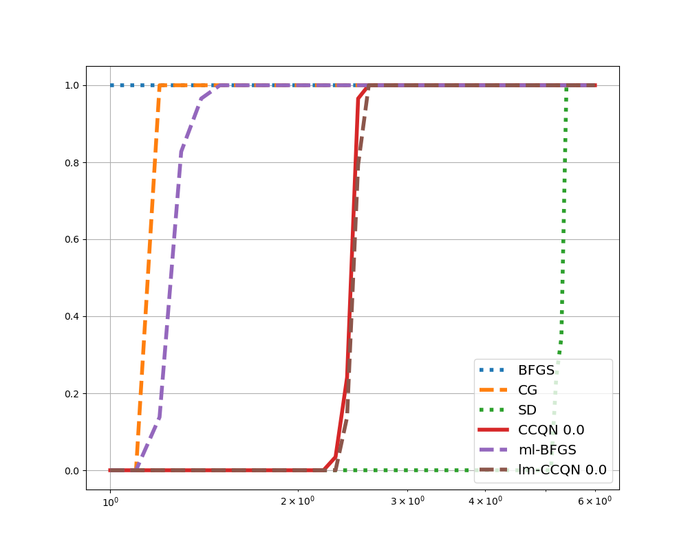
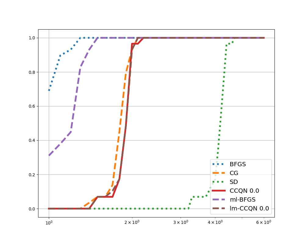
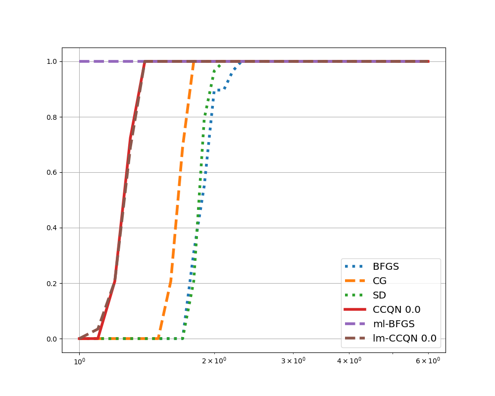
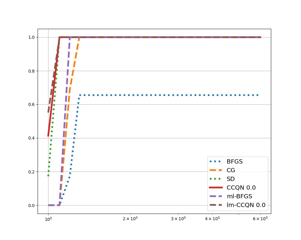
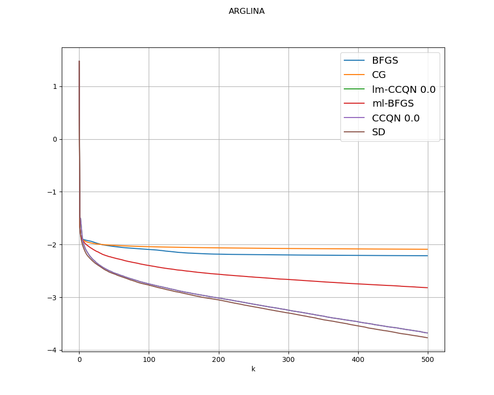
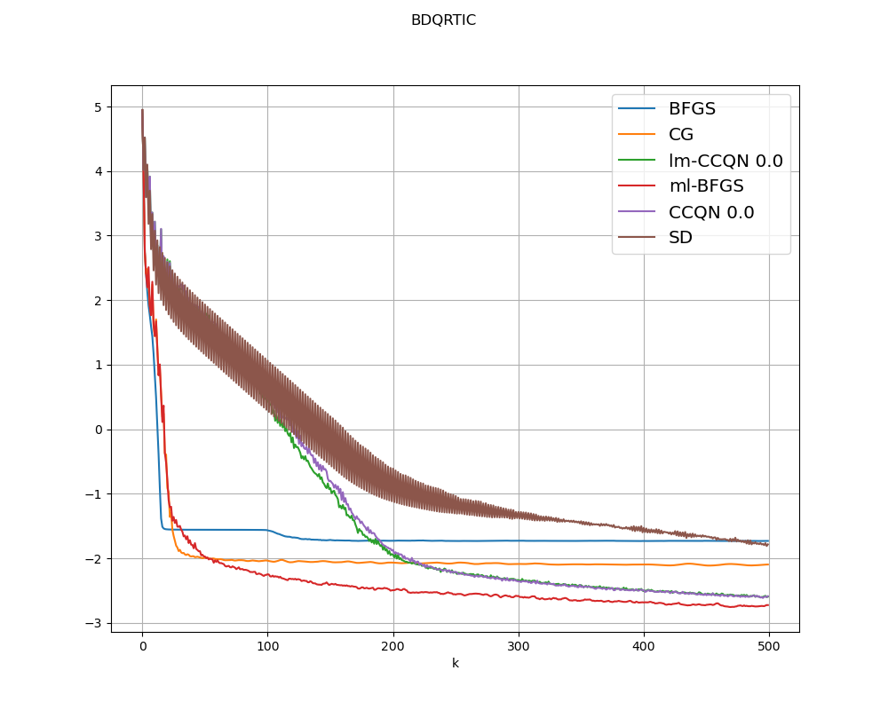
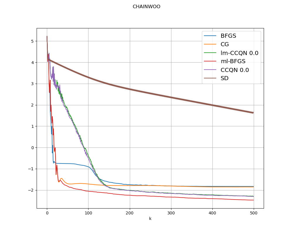
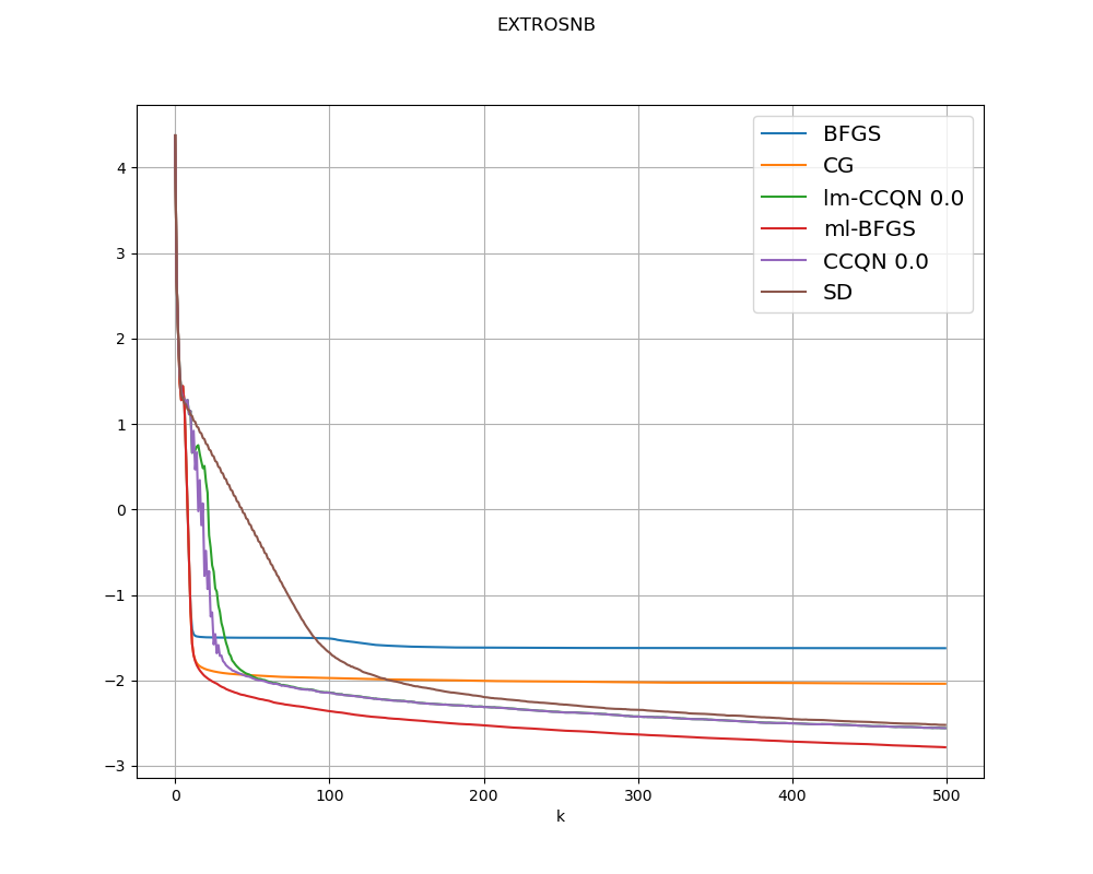
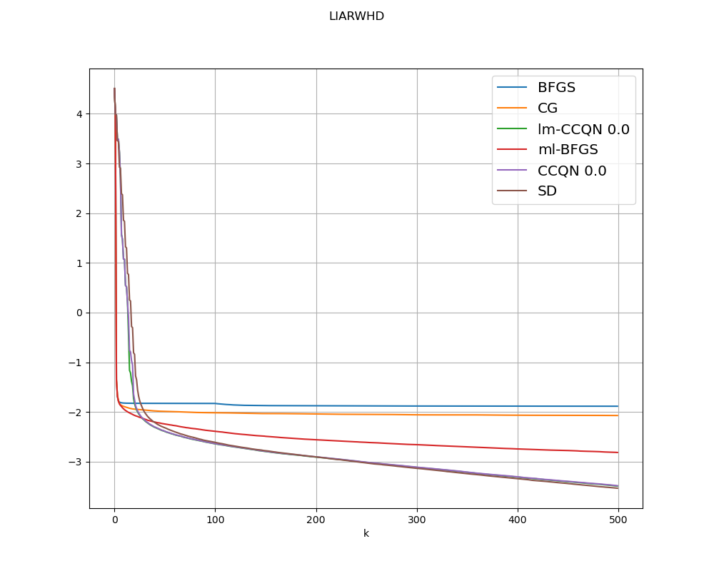
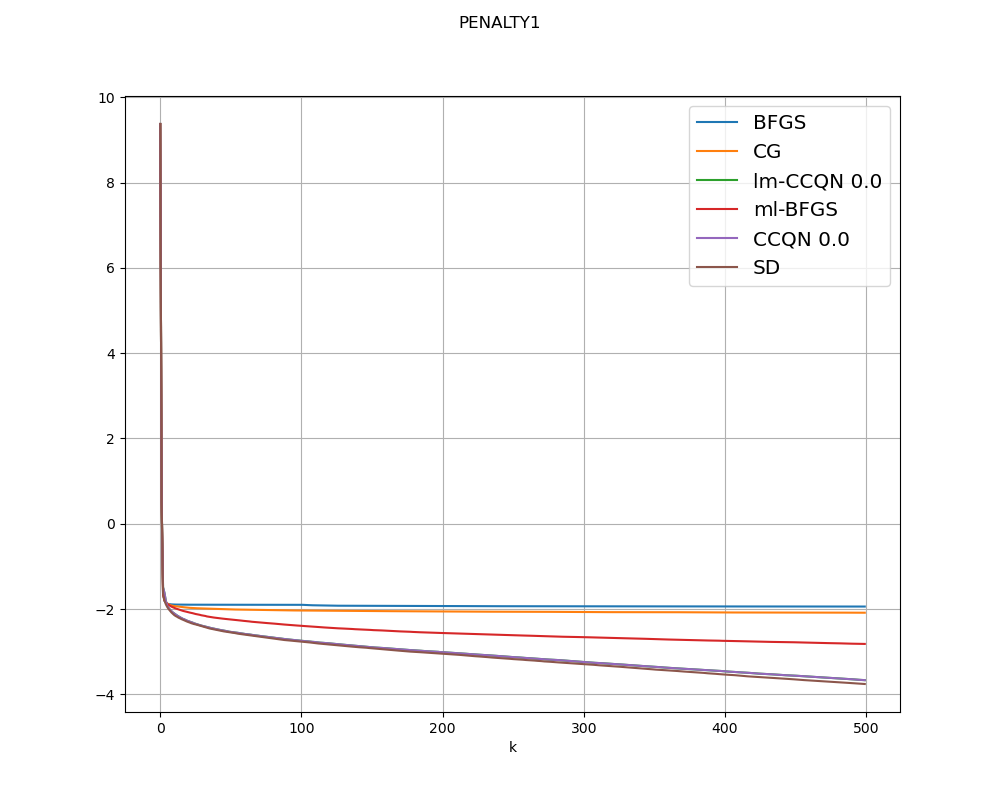
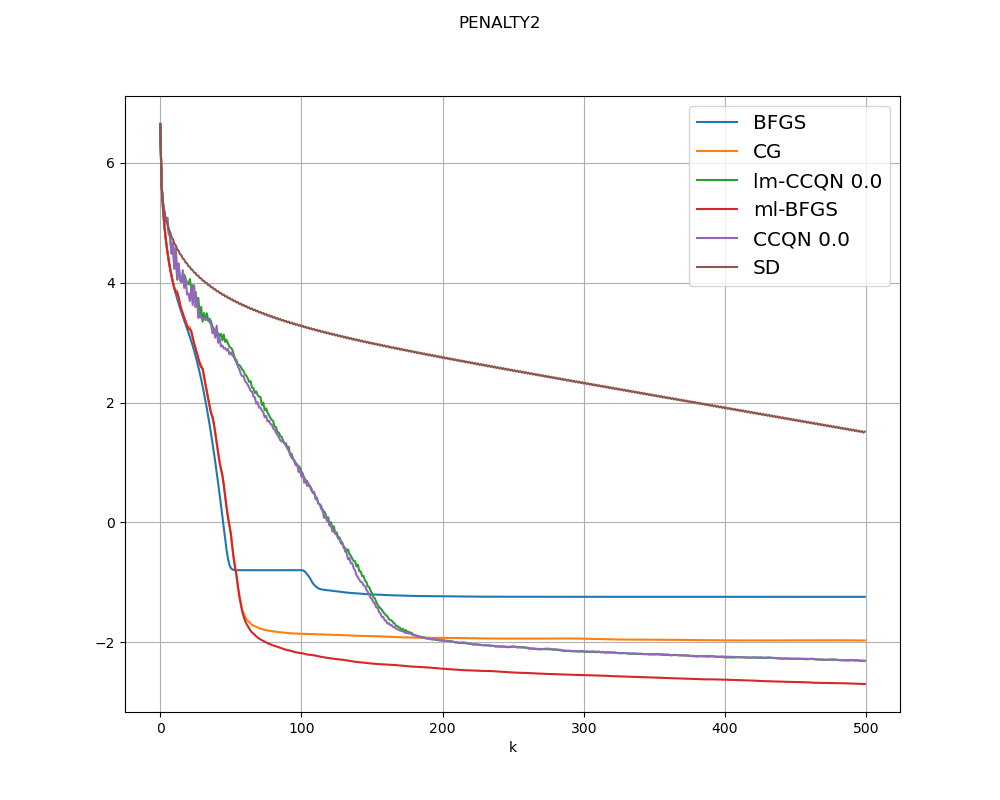
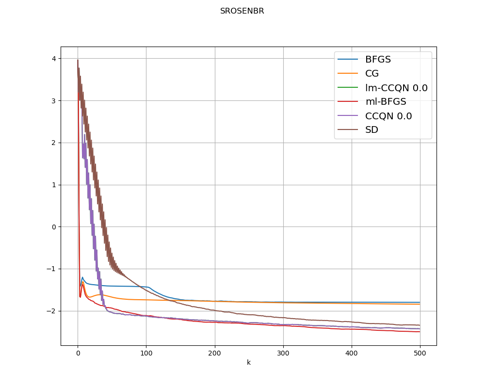
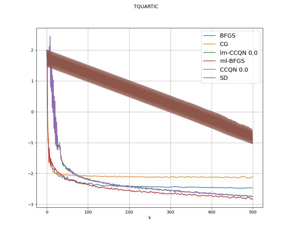
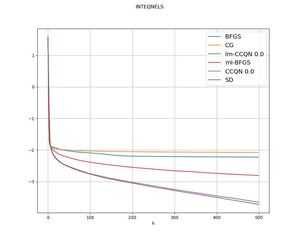
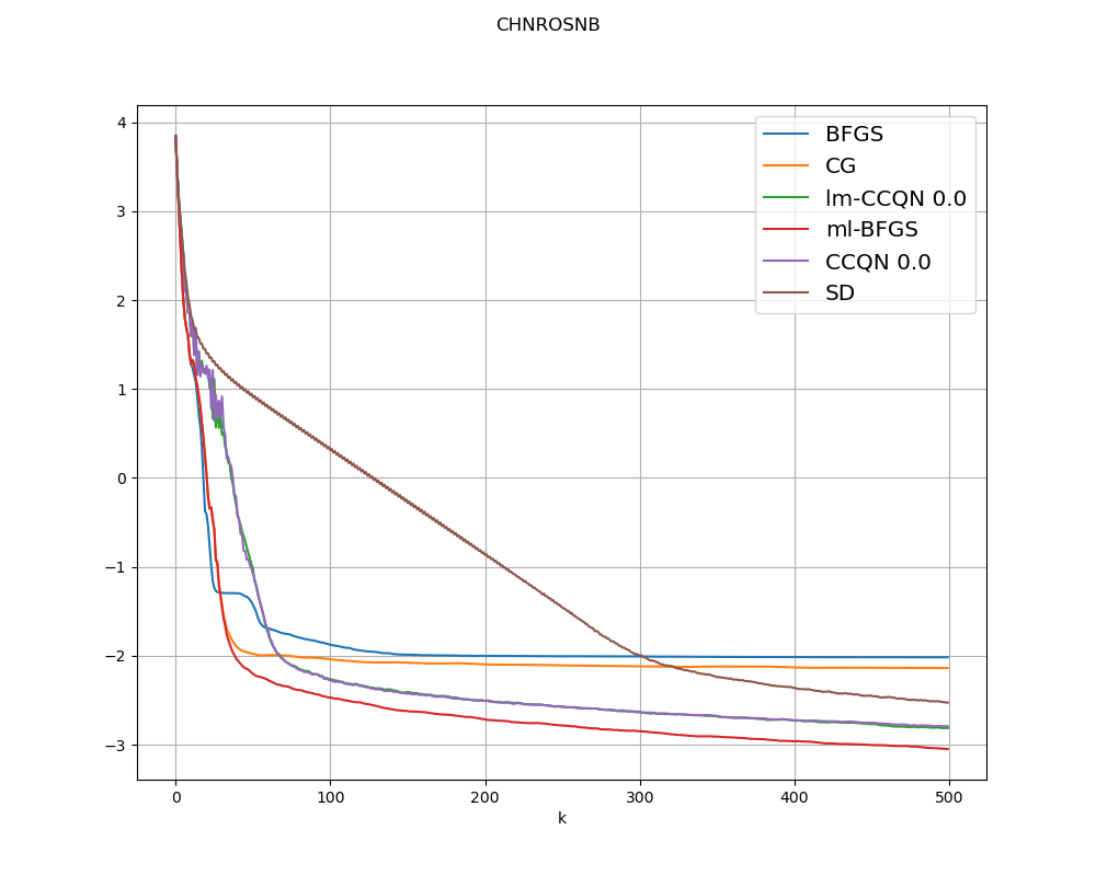
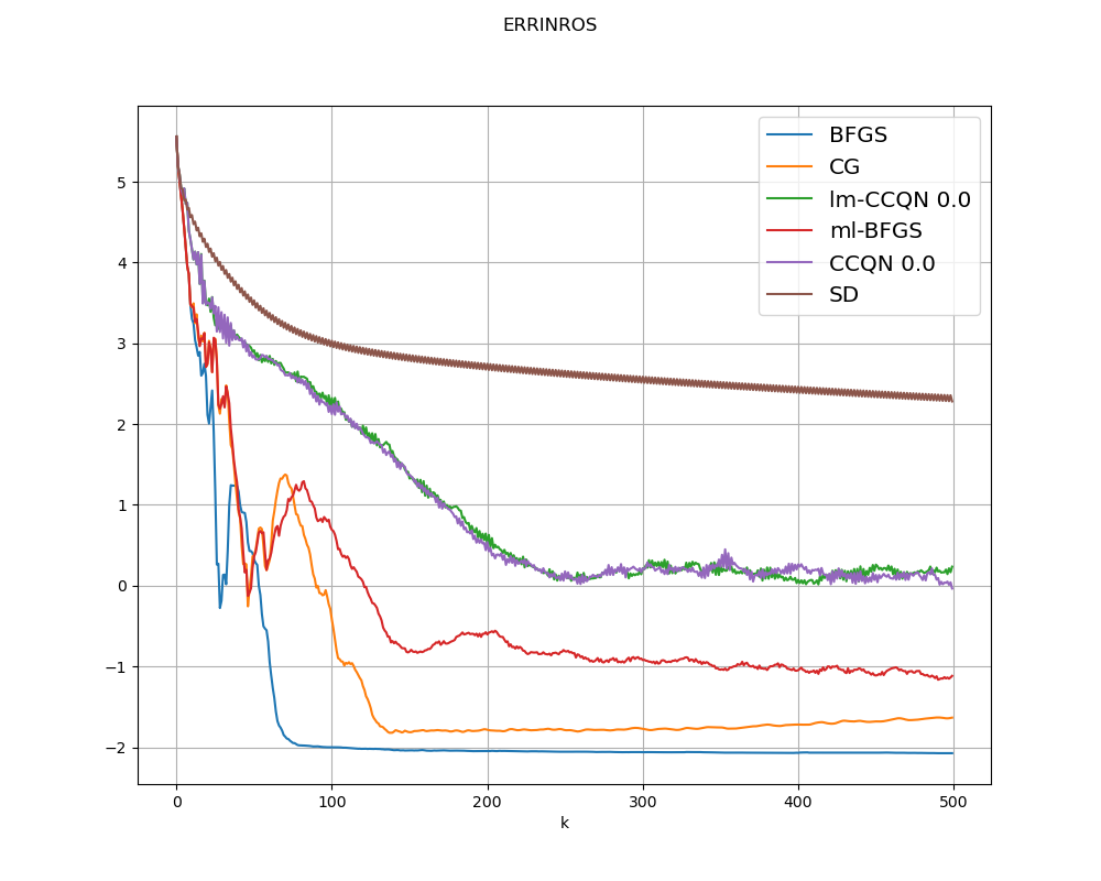
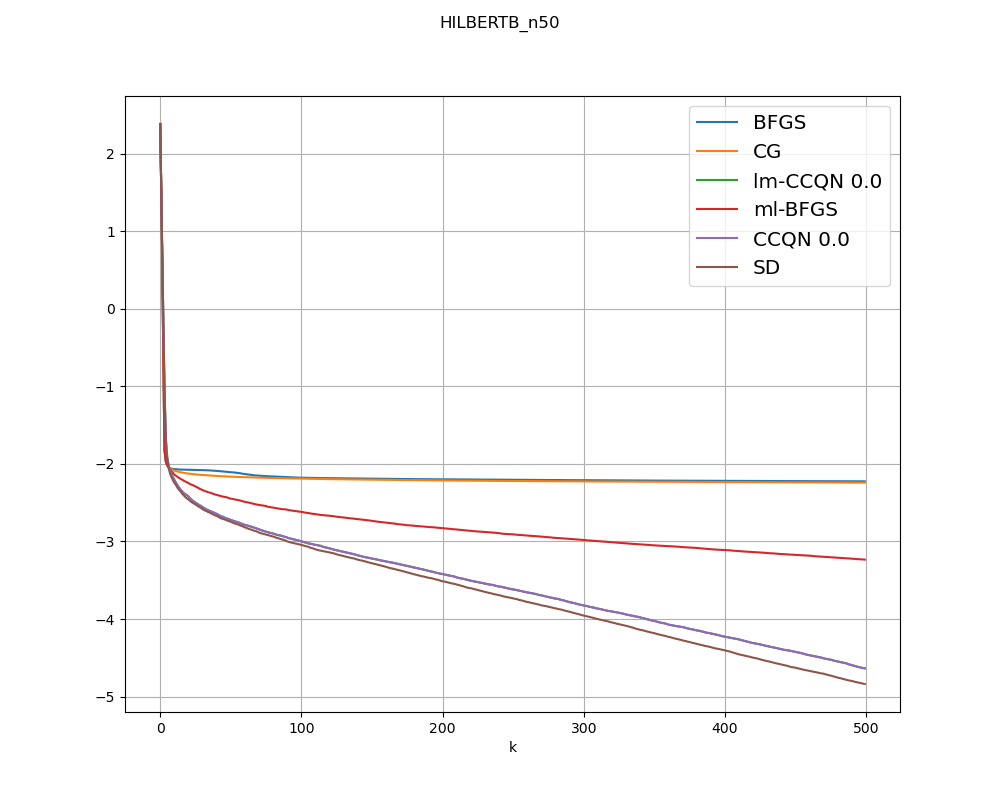
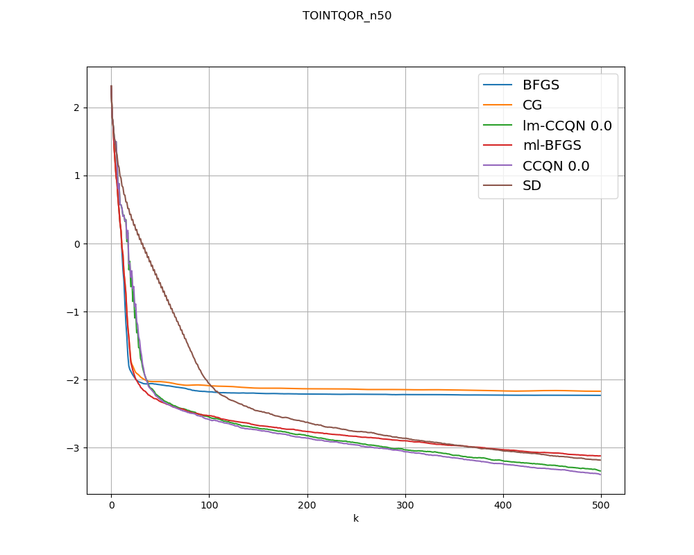
Figure 4 shows the performance profiles of different methods solving CUTEst problems under different tolerance levels. We can observe that the performance of BFGS and CG can be good and SD performs worst among all the tested methods, when the tolerance level is larger than the noise variance. However, as shown in Figure 4 (d), SD can perform better than ml-BFGS, BFGS and CG. ml-BFGS can show its efficiency and effectiveness in most cases. CCQN and lm-CCQN present their robustness under different tolerance levels, and perform better when the tolerance level is close or smaller than the noise variance. When , CCQN and lm-CCQN perform best, with the latter being slightly ahead.
When the tolerance level becomes much smaller, the performance profile of each method will depend on the problem, except CCQN and lm-CCQN. The ml-BFGS method will not always be the best, while the performances of CCQN and lm-CCQN are among the top three methods, which shows their robustness if the noise variance is larger the tolerance level. This behaviour can be observed in Appendix A for each individual problem.
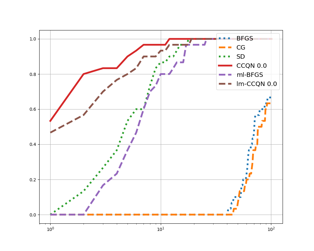
Figure 5 the performance profiles of the minimum gradient norm found in the CUTEst set of problems with different seeds. CCQN is able to obtain the minimum value consistently, followed by the lm-CCQN, SD and ml-BFGS (in that order), while BFGS and CG perform worst than all the other studied methods. The chance-constrained methods were able to obtain the minimum value faster and more frequently, even if compared it to ml-BFGS which had a good performance across our previously shown profiles.
6 Conclusion
In this paper, we have studied low-rank quasi-Newton methods for minimizing a strictly convex quadratic function in a noisy framework. We have considered a memoryless BFGS method and compared to a BFGS method, the method of conjugate graddients and steepest descent. In order to potentially improve the performance of the low-rank quasi-Newton method, a chance constrained stochastic optimization model has also been formulated. The secant condition is here replaced by solving a one-dimensional convex quadratic programming problem. The proposed chance constrained model, which can be solved effectively by sample average approximation method or scenario approach, has been proven to provide a descent search direction with a high probability in the random noisy framework, while the deterministic model may fail to provide a descent direction, if the noise level is large.
In the numerical experiments, we compare classical methods and the proposed chance constrained model in a noisy setting. Results of ml-BFGS and CCQN show promise when solving problems with uncertainty in the gradient, however the latter is more consistent and its performance appear to be independent of the problem, while the former does not. The performance of chance-constrained model (and its different iterations) appears to be in the top three in terms of convergence speed under different tolerance thresholds. Furthermore, while studying the behaviour of all the models, the minimal value of gradient norm was consistently found by the approach based on chance constrained model. Therefore, we believe that the usage of more advanced solving algorithms than the one presented (i.e. stochastic inexact linesearch) could further improve the results presented in this paper.
Finally, our intention is to investigate the behavior and the interplay between quality and robustness of the low-rank quasi-Newton method, especially in the case of large noise and multiple copies of gradients. Both the theoretical and numerical results show that we can gain the robustness and accuracy of the computed solution with the chance constrained model, although the computational cost can be high. This shows the potential to be further considered and explored in convex optimization problems.
References
- [AX18] S. Ahmed and W. Xie. Relaxations and approximations of chance constraints under finite distributions. Mathematical Programming, 170(1), 43–65, 2018.
- [BHdMM+16] J. Barrera, T. Homem-de Mello, E. Moreno, B. K. Pagnoncelli, and G. Canessa. Chance-constrained problems and rare events: an importance sampling approach. Mathematical Programming, 157(1), 153–189, 2016.
- [BHNS16] R. H. Byrd, S. L. Hansen, J. Nocedal, and Y. Singer. A stochastic quasi-Newton method for large-scale optimization. SIAM Journal on Optimization, 26(2), 1008–1031, 2016.
- [BNT16] A. S. Berahas, J. Nocedal, and M. Takac. A multi-batch L-BFGS method for machine learning. In D. D. Lee, M. Sugiyama, U. V. Luxburg, I. Guyon, and R. Garnett, editors, Advances in Neural Information Processing Systems 29 (NIPS 2016), volume 29, 2016.
- [DW84] J. E. Dennis and H. F. Walker. Inaccuracy in quasi-Newton methods - local improvement theorems. Mathematical Programming Study, 22(DEC), 70–85, 1984.
- [EF21] D. Ek and A. Forsgren. Exact linesearch limited-memory quasi-Newton methods for minimizing a quadratic function. Computational Optimization and Applications, 79(3), 789–816, 2021.
- [FO18] A. Forsgren and T. Odland. On exact linesearch quasi-Newton methods for minimizing a quadratic function. Computational Optimization and Applications, 69(1), 225–241, 2018.
- [GOT15] N. I. M. Gould, D. Orban, and P. L. Toint. CUTEst: a constrained and unconstrained testing environment with safe threads for mathematical optimization. Computational Optimization and Applications, 60(3), 545–557, 2015.
- [LMH15] A. Lucchi, B. McWilliams, and T. Hofmann. A variance reduced stochastic Newton method. Preprint arXiv:1503.08316 [cs.LG], 2015.
- [MNJ16] P. Moritz, R. Nishihara, and M. Jordan. A linearly-convergent stochastic L-BFGS algorithm. In Artificial Intelligence and Statistics, pages 249–258. PMLR, 2016.
- [MR13] A. Mokhtari and A. Ribeiro. Regularized stochastic BFGS algorithm. In 2013 IEEE Global Conference on Signal and Information Processing, pages 1109–1112. IEEE, 2013.
- [MR15] A. Mokhtari and A. Ribeiro. Global convergence of online limited memory BFGS. The Journal of Machine Learning Research, 16(1), 3151–3181, 2015.
- [Saa03] Y. Saad. Iterative methods for sparse linear systems. Society for Industrial and Applied Mathematics, Philadelphia, PA, 2003.
- [SDR14] A. Shapiro, D. Dentcheva, and A. Ruszczyński. Lectures on stochastic programming: modeling and theory. SIAM, Philadelphia, 2014.
- [SXBN20] H.-J. M. Shi, Y. Xie, R. Byrd, and J. Nocedal. A noise-tolerant quasi-Newton algorithm for unconstrained optimization. Preprint arXiv:2010.04352 [math.OC], 2020.
- [XBN20] Y. Xie, R. H. Byrd, and J. Nocedal. Analysis of the BFGS method with errors. SIAM Journal on Optimization, 30(1), 182–209, 2020.
Appendix A Average log norms gradients of the CUTEst problems
In this section, the average log norm of each CUTEst problem is presented. The objective is to make evident the difference between problems as stated in the experiment section 5.2. All of these results are presented for .