Phase engineering of chirped rogue waves in Bose–Einstein condensates with a variable scattering length in an expulsive potential

Abstract

We consider a cubic Gross-Pitaevskii (GP) equation governing the dynamics of Bose-Einstein condensates (BECs) with time-dependent coefficients in front of the cubic term and inverted parabolic potential. Under a special condition imposed on the coefficients, a combination of phase-imprint and modified lens-type transformations converts the GP equation into the integrable Kundu-Eckhaus (KE) one with constant coefficients, which contains the quintic nonlinearity and the Raman-like term producing the self-frequency shift. The condition for the baseband modulational instability of CW states is derived, providing the possibility of generation of chirped rogue waves (RWs) in the underlying matter-wave (BEC) model. Using known RW solutions of the KE equation, we present explicit first- and second-order chirped RW states. The chirp of the first- and second-order RWs is independent of the phase imprint. Detailed solutions are presented for the following configurations: (i) the nonlinearity exponentially varying in time; (ii) time-periodic modulation of the nonlinearity; (iii) a stepwise time modulation of the strength of the expulsive potential. Singularities of the local chirp coincide with valleys of the corresponding RWs. The results demonstrate that the temporal modulation of the s-wave scattering length and strength of the inverted parabolic potential can be used to manipulate the evolution of rogue matter waves in BEC.

Keywords: Chirp rogue wave; Bose-Einstein condensate; Kundu-Eckhaus equation; Gross-Pitaevskii equation; nonlinear Schrödinger equation

$\mathcal{DEDICATION}$: The first author, E. Kengne, dedicates this work to his brother, Sir Philippe Wambo

I Introduction

Extensive research work on nonlinear dynamics of atomic matter waves in Bose-Einstein condensates (BECs), such as dark 1 ; 2 ; 6 bright 6 ; 7 ; 8 , and breather breather1 ; breather2 solitons, rogue waves (RWs) 9 ; 10 , gap solitons and other coherent modes in optical lattices 11 ; Morsch , four-wave mixing 12 , and, most recently, quantum droplets in binary Petrov ; binary and dipolar dipolar BEC set these topics at the forefront of current experimental and theoretical studies in soft-matter physics and nonlinear science. A commonly adopted dynamical model of BEC is the Gross-Pitaevskii (GP) equation (including the Lee-Huang-Yang corrections that account for the beyond-mean-field effects helping to stabilize quantum droplets Petrov ). In the ideal one-dimensional (1D) form, which does not include losses, an external potential, and variable coefficients, the GP equation is tantamount to the classical integrable nonlinear Schrödinger (NLS) equation, which produces commonly known exact solutions for solitons and elastic interactions between them Zakharov ; 21 . Nevertheless, some specially designed integrable models admit exact solutions for fusion and fission of solitons 15 ; 16 ; we .

Similar to other nonlinear media, BECs may support the creation of rogue waves (RWs) Konotop , i.e., peaks spontaneously emerging on top of an unstable CW (continuous-wave, i.e., constant-amplitude) modulationally unstable background, and disappearing afterwards mi1 ; mi2 ; mi3 . Generally, rogue waves are known as waves which suddently appear in the oceans that can reach amplitudes more than twice the value of ignificant wave height jul1 . As far as Bose-Einstein condensates are concerned a sudden increase of peaks in the condensate clouds is very similar to the nature of appearance of high peaks in the open ocean jul1a . Mathematically, rational solutions of some nonlinear partial differential equations such as the NLS equation play a major role in the theory of rogue waves jul2 . Motivated by the above observation, we aim to address in this work, the dynamics of chirped rogue matter waves in the framework of the GP equation with a time-varying atomic scattering length, which determines the coefficient in front of the cubic term, and a time-dependent strength of the parabolic potential. The analysis is performed with the help of the phase-engineering technique 17 ; we , which imposes a phase imprint onto the BEC’s mean-field wave function. By means of this technique, we engineer the imprinted phase which makes it possible to transform the cubic GP equation into one including the cubic-quintic nonlinearity and a self-frequency-shift term. In particular, the quintic term may account for effects of three-body collisions in BEC 20 ; quintic ; 17 , as well as higher-order nonlinearity in optics 29 ; Reyna .

In the physically important case of the cigar-shaped BECs, the GP equation reduces to the 1D NLS equation with the external potential 6 ; 18 :

$$i\frac{\partial\psi(x,t)}{\partial t}+\frac{\partial^{2}\psi(x,t)}{\partial x^{2}}+2a(t)\left|\psi(x,t)\right|^{2}\psi(x,t)-k(t)x^{2}\psi(x,t)=0.$$ (1)

Here, $\psi(x,t)$ is the normalized mean-field wave function, time $t$ and coordinate $x$ are measured in units $2/\omega_{\bot}$ and $a_{\bot}$, where $a_{\bot}=\sqrt{\hslash/(m\omega_{\bot})}$ is the harmonic-oscillator lengths of the transverse confining potential with frequency $\omega_{\perp}$, $m$ is the atomic mass, and $\omega_{0}$ is the frequency of the longitudinal trapping potential, $k=2\omega_{0}^{2}/\omega_{\bot}^{2}\ll 1$ being its relative strength, which may be a time-dependent parameter we . The nonlinearity coefficient may also be made a function of time by means of the Feshbach-resonance (FR) management, if FR is imposed by a variable magnetic filed book . In this case, the nonlinearity coefficient in Eq. (1) is $a(t)=\left|a_{s}(t)\right|/a_{B}$, where $a_{B}$ is the Bohr radius, and $a_{s}(t)<0$ is the s-wave scattering length of collisions between attractively interacting atoms. In the experiment, bright solitons were created by utilizing FR to switch the sign of the s-wave scattering length from positive to negative 8 values. In the GP equation (1), the 1D wave function $\psi(x,t)$ is related to the original 3D one, $\Psi(\mathbf{r},t)$, by expression

$$\Psi(\mathbf{r},t)=\frac{1}{\sqrt{2\pi a_{B}a_{\bot}}}\psi\left(\frac{x}{a_{\bot}},\frac{\omega_{\bot}t}{2}\right)\exp\left(-i\omega_{\bot}t-\frac{x^{2}+y^{2}}{2a_{\bot}}\right).$$ (2)

The 3D and 1D equations are very different in terms of their stability. In the true 1D system, the collapse does not occur with the increase of the number of atoms. However, the realistic 1D limit is not tantamount to the ideal NLS equation, the deviation from which makes the collapse possible NJP ; breather2 . Nevertheless, in Ref. 7 it was demonstrated that, in a safe range of parameters, one can avoid the collapse of the condensates, while exponentially increasing $a(t)$ by means of the FR management. The repulsive three-body interatomic interactions, which are represented by the above-mentioned quintic term added to the GP equation, can also enhance the stability of BEC 20 ; quintic ; 17 . The inclusion of the latter term allows one to generate high-density BEC, while retaining the one-dimensionality of the system without severely restricting to the parametric domain.

Parameter $a(t)$ of the two-body interatomic interaction being time-dependent, Eq. (1) can be used to describe the control and management of BEC book ; we . As concerns a possibility to design an integrable version of Eq. (1), Kumar et al. 17 had produced a Lax pair associated with a specific form of the cubic-quintic GP equation, and had thus constructed bright solitons employing a gauge-transformation method. It was thus demonstrated that, for attractive three-body interactions, solitons of the cubic-quintic GP equation with an exponentially increasing scattering length and constant potential strength differ from those of the cubic GP equation by an additional phase, while the density of the condensates remains the same.

Proceeding to chirped solitons, it is relevant to mention that, because of their ability to produce very narrow outputs, chirped pulses are particularly useful in photonics, for the design of fiber-optic amplifiers, optical pulse compressors, and soliton-based communications links 22 . Pulses with the linear chirp and a hyperbolic-secant-amplitude profile were investigated numerically and analytically 23 . The existence of chirped soliton-like solutions of the cubic-quintic NLS equation without an external potential was reported too 24 . Within the framework of a generalized NLS equation containing the group-velocity dispersion, Kerr and quintic nonlinearity, and self-steepening effect, Chen et al. 25 had investigated the super-chirped RW dynamics in optical fibers, using the nonrecursive Darboux-transformation technique. Most recently, Mouassom et al. 26 have combined the similarity transformation and the use of a direct ansatz to solve analytically an inhomogeneous chiral NLS equation with modulated coefficients. They have also investigated the RW propagation with a chirped structure. The existence of chirped solitons in BEC models with in external potentials was reported too 27 .

The main purpose of this work is to map the cubic GP Eq. (1) into an integrable cubic-quintic NLS equation including a self-frequency shift term, which is known as the Kundu-Eckhaus equation 300 . Using solutions of the KE equation makes it possible to generate chirped RWs in BEC with both two- and three-body interatomic interactions in the external harmonic-oscillator trap by suitably engineering the phase imprint imposed on the wave function governed by Eq. (1). The rest of the work is organized as follows. In Section II, we combine the phase engineering technique with a modified lens-type transformation to map the cubic GP Eq. (1) into an integrable cubic-quintic NLS equation with a self-frequency shift term, which is then used to produce analytical chirped RW solutions for BEC with the time-varying atomic scattering length in an external parabolic potential. In Section III, the obtained exact solutions are used to investigate the effects of the three-body interatomic interactions on the chirped RWs. Main results of the work are summarized in Section IV.

II Phase engineering and chirped solutions

II.1 The transformations

To derive analytical chirped-wave solutions of Eq. (1), we combine the phase-engineering technique 17 and a modified lens-type transformation, by means of the following ansatz:

$$\psi(x,t)=\frac{1}{\sqrt{\ell}}\Phi(X,T)\exp\left[i\left\{\alpha(t)x^{2}-2\theta(x,t)\right\}\right],$$ (3)

where $\Phi(X,T)$ is a new complex wave function, $T=T(t)$, $\ell=\ell(t)$ and $\alpha(t)$ are real functions of time $t$, $X\equiv x/\ell(t)$, and $\theta(x,t)$ is the phase imprint, related to $\Phi(X,T)$ as follows:

$$\frac{\partial\theta}{\partial x} = -\frac{a_{3}}{4\ell}\left|\Phi\right|^{2},$$ (4a)

$$\frac{\partial\theta}{\partial t} = i\frac{a_{3}}{4}\left[\frac{1}{\ell^{2}}\left(\Phi\frac{\partial\Phi^{\ast}}{\partial X}-\Phi^{\ast}\frac{\partial\Phi}{\partial X}\right)-4ix\alpha(t)\frac{1}{\ell}\left|\Phi\right|^{2}\right]+\frac{\allowbreak 4a_{1}+a_{3}^{2}}{8\ell^{2}}\left|\Phi\right|^{4}.$$ (4b)

Here, $$a_{1} a_{3} \alpha(t)=0 \ell(t)=1$$ and are two real parameters of the phase engineering technique. In the special case when and , the substitution of ansatz (3) with the phase imprint defined by Eqs. (4a) and (4b) transforms the cubic GP Eq. (1) into a cubic-quintic GP equation with a cubic derivative term 17 .

In this work, we focus on the general situation with $\alpha(t)\neq 0$. We then demand that

$$\frac{dT}{dt} = \frac{1}{\ell^{2}},$$ (5a)

$$\frac{1}{\ell}\frac{d\ell}{dt}-4\alpha = 0,$$ (5b)

$$\frac{d\alpha}{dt}+4\alpha^{2}+k(t) = 0.$$ (5c)

The choice of Eq. (5a) is made to preserve the scaling. Then, Eq. (1) in terms of rescaled variables $$X T$$ and is converted into the following cubic-quintic NLS equation with an additional cubic derivative term:

$$i\frac{\partial\Phi}{\partial T}+\frac{\partial^{2}\Phi}{\partial X^{2}}+2\ell a(t)\left|\Phi\right|^{2}\Phi+\allowbreak a_{1}\left|\Phi\right|^{4}\Phi+ia_{3}\left(\frac{\partial}{\partial X}\left|\Phi\right|^{2}\right)\Phi=0,$$ (6)

where $a_{1}$ and $2\ell a(t)>0$ represent the quintic and cubic nonlinearities, respectively, and $a_{3}$ is the self-frequency shift coefficient. In the context of fiber optics, Eq. (6) may be used to model the propagation of ultrashort pulses in a single-mode optical fiber 28 . In that context, $T$ and $X$ are the propagation distance and retarded time, respectively, $2\ell a(t)$ is the coefficient of the cubic nonlinearity [in the optics counterpart of Eq. (5), this coefficient may then be rescaled into one multiplying the group-velocity dispersion (GVD) term, which is termed anomalous and normal GVD for $a(t)>0$ and $a(t)<0$, respectively] 29 ; 25 , and real $a_{3}$ is related to the fiber’s nonlinearity dispersion. In the context of BECs, Eq. (6) may be used as the GP equation including both two- and three-body interatomic interactions, with $2\ell a(t)$ and $a_{1}$ representing the strengths of these interactions, respectively. As mentioned by Kumar et al. in Ref. 17 , this way of engineering the phase imprint to generate a new integrable model is reminiscent of generating dark solitons in BEC by dint of phase imprinting 29a .

To provide integrability of Eq. (6) and exploit some known results of the integrable KE equation 300 , we adopt the linkage of strength $a_{1}$ of the three-body interactions to the self-frequency-shift parameter $a_{3}$, viz.,

$$a_{1}=a_{3}^{2}/4,$$ (7)

and impose condition

$$\ell(t)=\frac{a_{2}}{2a(t)},\text{ \ }$$ (8a)

where $$a_{2} k(t) a(t)$$ is an arbitrary positive real parameter. We then obtain from Eqs. (5a)–(5c) that the potential’s and nonlinearity strengths, and , must satisfy a constraint,

$$\frac{d}{dt}\left(\frac{1}{a}\frac{da}{dt}\right)-\left(\frac{1}{a}\frac{da}{dt}\right)^{2}-4k(t)=0,$$ (8b)

while $$T(t) \alpha(t)$$ and must be defined as

$$T(t)=\frac{4}{a_{2}^{2}}\int_{0}^{t}a^{2}(z)dz,\text{ }\alpha(t)=-\frac{1}{4a}\frac{da}{dt}.$$ (8c)

Note that Eq. (8b) is a Riccati type equation for function $$a^{-1}da/dt a(t)$$. Regardless of what is, as long as condition (8b) holds the underlying cubic GP equation (1) is integrable. Henceforth, we call equation (8b) the integrability condition for the cubic equation (1) (condition (7) is not by itself necessary for selecting the integrable version of Eq. (1)). It is also important to mention that the Painlevé singularity-structure analysis performed on Eq. (1) confirms that the same condition (8b) is a necessary integrability conditions. Finally, we note that the solution based on ansatz (3) provides flexibility to generate new structures related to chirped RWs, which may be relevant for experiments with BEC.

By choosing the self-frequency shift coefficient as $a_{3}=-2\sqrt{2a_{2}}\beta$ and using transformation $\tau=\left(a_{2}/2\right)T,$ $\zeta=\sqrt{a_{2}/2}X$, Eq. (6), subject to condition (8a), reduces to the integrable Kundu-Eckhaus equation 300 ,

$$i\frac{\partial\Phi}{\partial\tau}+\frac{\partial^{2}\Phi}{\partial\zeta^{2}}+2\left|\Phi\right|^{2}\Phi+4\beta^{2}\left|\Phi\right|^{4}\Phi-4i\beta\left(\frac{\partial}{\partial\zeta}\left|\Phi\right|^{2}\right)\Phi=0,$$ (9)

which finds applications to nonlinear optics, quantum field theory, and matter waves 300 ; 30 ; 30a ; here, $\beta$ is a real parameter of arbitrary sign. Most recently, Kengne and Liu in Ref. 17 have derived the cubic-quintic NLS equation (6) to engineer RWs in a modified Nogochi nonlinear electric transmission network 31 .

As mentioned by Kumar et al. 17 , the last term in Eq. (9) offsets the modulation instability driven the three-body interactions. As pointed out in Ref. 20 , strength $4\beta^{2}$ of the three-body interaction in Eq. (9) is usually small in comparison to the strength of the two-body interaction, which is represented by cubic term in Eq. (9). Accordingly, we here set $2\beta^{2}\equiv\chi_{0},$ with $0\leq\chi_{0}<1$, hence $\beta$ takes values $\left|\beta\right|<1/\sqrt{2}\approx 0.70711$. Because the strength of the three-body interaction is related to that of the binary interaction, $\beta$ may be controlled by the tuning the s-wave scattering length, with the help of FR.

Lastly, we note that relation (3) implies that solutions of the cubic-quintic NLS equation (6) has the same density structure as solutions of the cubic GP equation (1), differing from them by the phase pattern.

II.2 Baseband modulational instability analysis

It is known that the modulational instability (MI) is the basic mechanism that may lead to the excitation of RW in nonlinear media mi1 ; mi2 ; mi3 . Appearing in many nonlinear dispersive systems, MI is associated with the growth of spatially periodic perturbations added to an unstable CW background, and indicates that, due to the interplay between the nonlinearity and dispersive effects, a small perturbation may lead to breakup of the CW into a train of localized waves mi4 . Most recently, it has been revealed that not every kind of MI necessarily leads to the generation of RWs, and, generally, it is the baseband MI that plays such a pivotal role in RW generation mi1 ; mi5 . Baseband MI implies that the CW background may be unstable against perturbations with infinitesimally small wavenumbers mi1 .

We begin with the CW solution of Eq. (6) that, under condition (8a), amounts to

$$\Phi_{0}(X,T)=\rho_{0}\exp\left[i\left\{\Omega_{0}X+\left(a_{2}\rho_{0}^{2}+\allowbreak a_{1}\rho_{0}^{4}-\Omega_{0}^{2}\right)T\right\}\right],$$ (10)

where $\rho_{0}$ and $\Omega_{0}$ are, respectively, the amplitude and wavenumber, while real $\widetilde{\omega}=$ $a_{2}\rho_{0}^{2}+\allowbreak a_{1}\rho_{0}^{4}-\Omega_{0}^{2}$ is the frequency. To address the baseband MI, we add small modulational perturbations to the CW solution (10):

$$\Phi(X,T)=\Phi_{0}(X,T)\left\{1+b_{1}\exp\left[i\Omega\left(X-KT\right)\right]+b_{2}^{\ast}\exp\left[-i\Omega\left(X-K^{\ast}T\right)\right]\right\},$$ (11)

where $b_{1}$ and $b_{2}$ are two small complex amplitudes, $\Omega$ and $\Omega K$ are, respectively, the wavenumber and frequency of the modulation, and $\ast$ stands for the complex conjugate. The MI emerges when $K$ becomes complex. Substituting Eq. (11) into Eq. (6) under condition (8a) and linearizing the resulting equation with respect to $b_{1}$ and $b_{2}$, we obtain a linear homogeneous algebraic system for amplitudes $b_{1}$ and $b_{2}$:

$$\left\{\begin{array}[]{c}\left(K\Omega-2\Omega\Omega_{0}-\Omega^{2}+a_{2}\rho_{0}^{2}+2a_{1}\rho_{0}^{4}-a_{3}\rho_{0}^{2}\Omega\right)b_{1}+\left(a_{2}\rho_{0}^{2}+2a_{1}\rho_{0}^{4}-a_{3}\rho_{0}^{2}\Omega\allowbreak\right)b_{2}=0,\\ \left(a_{2}\rho_{0}^{2}+2a_{1}\rho_{0}^{4}+a_{3}\rho_{0}^{2}\Omega\right)b_{1}+\left(-K\Omega+2\Omega\Omega_{0}-\Omega^{2}+a_{2}\rho_{0}^{2}+2a_{1}\rho_{0}^{4}+a_{3}\rho_{0}^{2}\Omega\right)b_{2}=0.\end{array}\right.$$ (12)

This system has a nontrivial solution if $\Omega$ and $K$ satisfy the linear dispersion relation,

$$\Omega^{2}\left[\allowbreak\left(\allowbreak K-2\Omega_{0}-a_{3}\rho_{0}^{2}\right)^{2}-\Omega^{2}+\rho_{0}^{2}\left(\allowbreak 2a_{2}+\left(4a_{1}-a_{3}^{2}\right)\rho_{0}^{2}\right)\right]=0.$$ (13)

It is seen from Eq. (13) that complex $K$ appears for $\Omega\rightarrow+0$ under the condition that

$$\allowbreak 2a_{2}+\left(4a_{1}-a_{3}^{2}\right)\rho_{0}^{2}>0.$$ (14)

In what follows below, condition (14) is referred to as the condition of the baseband MI for Eq. (6) under condition (8a). It is obvious that inequality (14) holds only for $a_{2}>0$. In other words, RWs may be excited in Eq. (6) by the MI under condition (14) only in the case of the self-focusing nonlinearity, with $a_{2}>0$. Specifically, this condition is satisfied for the KE equation (9) in which $a_{2}=2>0$ and $a_{1}=a_{3}^{2}/4$. For any CW amplitude $\rho_{0}$ that satisfies the baseband-MI condition (14), Eq. (13) yields $K=2\Omega_{0}+a_{3}\rho_{0}^{2}\pm i\sqrt{\left(\allowbreak 2a_{2}+\left(4a_{1}-a_{3}^{2}\right)\rho_{0}^{2}\right)\rho_{0}^{2}-\Omega^{2}}$. Therefore, the growth rate (gain) of the baseband MI is

$$\Gamma(\Omega)=\Omega\sqrt{\left[\allowbreak 2a_{2}+\left(4a_{1}-a_{3}^{2}\right)\rho_{0}^{2}\right]\rho_{0}^{2}-\Omega^{2}}\text{, for \ }0\leq\Omega\leq\rho_{0}\sqrt{2a_{2}+\left(4a_{1}-a_{3}^{2}\right)\rho_{0}^{2}}.$$ (15)

Using Eq. (15), one can obtain the MI map in the plane of $\left(\Omega,\rho_{0}\right)$. Figure 1 displays the map associated with Eq. (6) under condition (8a). It is seen from the figure that the baseband MI occurs not at all values of $\rho_{0}$, and the instability region expands as parameter $a_{1}$ increases. Note that Fig. 1(d) corresponds to the KE equation (9), and the associated MI boundary does not depend on $\beta$.

II.3 Chirped rogue waves

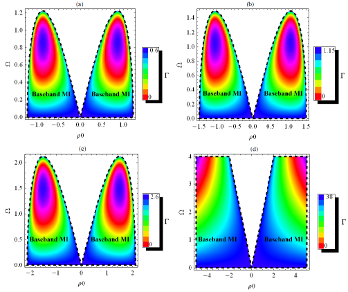
Figure 1: (Color online) MI (modulational instability) maps in the plane of $\Omega$ and $\rho_{0}$, as produced by Eq. (15) for $a_{2}=2,$ $a_{3}=-4\beta$ and four values of $a_{1}$: (a) $a_{1}=-2\beta^{2}$, (b) $a_{1}=0,$ (c) $a_{1}=2\beta^{2}$, and (d) $a_{1}=4\beta^{2}$, with $\beta=1/3$. Dashed lines show MI boundaries, defined by either $\Omega=\sqrt{\allowbreak 2a_{2}\rho_{0}^{2}+\left(4a_{1}-a_{3}^{2}\right)\rho_{0}^{4}}$ or $\Omega=0$.

Here, we aim to find exact chirped RW solutions of the cubic GP equation (1), under the integrability condition (8b). We limit ourselves to the situation when the condition $2a_{2}+\left(4a_{1}-a_{3}^{2}\right)\rho_{0}^{2}>0$ of the baseband MI is satisfied. Further, we consider only the case when the quintic-nonlinearity parameter $a_{1}$ in Eq. (6) is related to the self-frequency-shift one $a_{3}$ by Eq. (7), and then we choose the self-frequency-shift coefficient as $a_{3}=-2\sqrt{2a_{2}}\beta\neq 0$, so that Eq. (6) can be reduced to the integrable KE equation (9), with Fig. 1(d) showing the corresponding MI map. Then, we exploit the first-order and second-order RW solutions of Eq. (9) from 30a ; 31 to build the analytical first-order and second-order chirped RW solutions of the cubic GP Eq. (1). From the results obtained in Refs. 30a ; 31 , the first-order RW solution of Eq. (6) in the special case with $a_{1}=a_{3}^{2}/4=0$ and $a_{3}=-2\sqrt{2a_{2}}\beta\neq 0$ can be written as

$$\Phi(X,T) = \frac{4-D_{1}+8ia_{2}T}{D_{1}}\exp\left[i\left(-\beta\sqrt{2a_{2}}X+\frac{a_{2}\left(2+4\beta^{2}\right)}{2}T+\beta\sqrt{2a_{2}}\int\left|\frac{4-D_{1}+8ia_{2}T}{D_{1}}\right|^{2}dX\right)\right],$$ (16a)

$$D_{1} = 1+4a_{2}^{2}T^{2}+2a_{2}\left(X+2\sqrt{2a_{2}}\beta T\right)^{2},$$ (16b)

where $$a_{2}$$ is an arbitrary positive real parameter. Inserting Eq. (16a) into the ansatz (3) and using Eq. (8b) yields the following first-order RW solution of the cubic GP equation (1):

$$\psi(x,t) = \sqrt{\frac{2a(t)}{a_{2}}}\sqrt{\frac{\left(4-D_{1}\right)^{2}+64a_{2}^{2}T^{2}}{D_{1}^{2}}}\exp\left[i\left(\arctan\left[\frac{8a_{2}T}{4-D_{1}}\right]-\frac{1}{4a}\frac{da}{dt}x^{2}-2\beta\sqrt{\frac{2}{a_{2}}}a(t)x\right.\right.$$ (17a)

$$\left.\left.+\frac{2\left(2+4\beta^{2}\right)}{a_{2}}\int_{0}^{t}a^{2}(z)dz-2\theta(x,t)+2\beta\sqrt{\frac{2}{a_{2}}}a(t)\int\left|\frac{4-D_{1}+i8a_{2}T}{D_{1}}\right|^{2}dx\right)\right],$$

where $$D_{1}=D_{1}(X(x,t),T(t)) X=X(x,t) T=T(t)$$ is defined in Eq. (16b), with and given by Eq. (8c). The corresponding chirp is

$$\delta\omega=\frac{1}{2a}\frac{da}{dt}x-2a(t)\sqrt{\frac{2}{a_{2}}}\left(\beta+\frac{1}{\sqrt{2a_{2}}}\times\left.\frac{\partial}{\partial X}\arctan\left[\frac{8a_{2}T}{4-D_{1}}\right]\right|_{X=X(x,t),\text{ }T=T(t)}\right).$$ (17b)

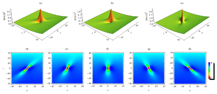
Figure 2: (Color online) Top panels: 3D density plots of the first-order RW (rogue wave) solution (17a) for different values of parameter $\beta$. (a): $\beta=-1/3$; (b): $\beta=0$; (c): $\beta=1/3$. Bottom panels: top views of the density distribution in the first-order RW solution (17a) for different values of $\beta$. (d): $\beta=-0.7$; (e): $\beta=-1/3$; (f): $\beta=0$; (g): $\beta=1/3$; (h): $\beta=0.7$. Other parameters are $r_{0}=0.25$ and $\lambda=0.02$.

To derive the second-order RW solution of the cubic GP equation (1), we apply the results from Ref. 30a for Eq. (9), leading to the following solution of Eq. (6):

$$\Phi(X,T)=\frac{F_{2}+iG_{2}}{D_{2}}\exp\left[i\left(-\beta\sqrt{2a_{2}}X+\frac{a_{2}\left(2+4\beta^{2}\right)}{2}T+\beta\sqrt{2a_{2}}\int\left|\frac{F_{2}+iG_{2}}{D_{2}}\right|^{2}dX\right)\right],$$ (18a)

where

$$F_{2} = 45-90a_{2}X^{2}-36a_{2}^{2}X^{4}+8a_{2}^{3}X^{6}-48a_{2}\sqrt{\frac{a_{2}}{2}}\left(15\beta+12\beta a_{2}X^{2}-4\beta a_{2}^{2}X^{4}\right)XT$$

$$-12a_{2}^{2}\left[392+60\beta^{2}+12a_{2}\left(5+12\beta^{2}\right)X^{2}-4a_{2}^{2}\left(1+20\beta^{2}\right)X^{4}\right]T^{2}$$

$$-128\beta a_{2}^{3}\sqrt{\frac{a_{2}}{2}}\left[9\left(5+4\beta^{2}\right)-2a_{2}\left(3+20\beta^{2}\right)X^{2}\right]XT^{3}$$

$$-48a_{2}^{4}\left[11+120\beta^{2}+48\beta^{4}-2a_{2}\left(1+20\beta^{2}\right)\left(1+4\beta^{2}\right)X^{2}\right]T^{4}$$

$$+768a_{2}^{5}\beta\sqrt{\frac{a_{2}}{2}}\left(1+4\beta^{2}\right)^{2}XT^{5}+64a_{2}^{6}\beta\left(1+4\beta^{2}\right)^{3}T^{6},$$

$$G_{2} = 24a_{2}\left(15+12a_{2}X^{2}-4a_{2}^{2}X^{4}\right)T-768a_{2}^{2}\beta\sqrt{\frac{a_{2}}{2}}\left(2a_{2}X^{3}-3X\right)T^{2}-192a_{2}^{3}$$ (18c)

$$\times\left[1-12\beta^{2}+2a_{2}\left(12\beta^{2}+1\right)X^{2}\right]T^{3}-3072a_{2}^{4}\beta\sqrt{\frac{a_{2}}{2}}\left(1+4\beta^{2}\right)XT^{4}-384a_{2}^{5}\left(1+4\beta^{2}\right)^{2}T^{5},$$

$$D_{2} = 9+54a_{2}X^{2}+12a_{2}^{2}X^{4}+8a_{2}^{3}X^{6}+48a_{2}\beta\sqrt{\frac{a_{2}}{2}}\left(4a_{2}^{2}X^{5}+4a_{2}X^{3}+9X\right)T$$

$$+12a_{2}^{2}\left[33+36\beta^{2}+12a_{2}\left(2\beta-1\right)\left(2\beta+1\right)X^{2}+4a_{2}^{2}\left(1+20\beta^{2}\right)X^{4}\right]T^{2}$$

$$+128a_{2}^{3}\sqrt{\frac{a_{2}}{2}}\left[3\beta\left(4\beta^{2}-3\right)X+2a_{2}\beta\left(3+20\beta^{2}\right)X^{3}\right]T^{3}$$

$$+48a_{2}^{4}\left[\left(4\beta^{2}-3\right)^{2}+2a_{2}\left(1+20\beta^{2}\right)\left(1+4\beta^{2}\right)X^{2}\right]T^{4}$$

$$+384\beta a_{2}^{5}\sqrt{2a_{2}}\left(1+4\beta^{2}\right)^{2}XT^{5}+64a_{2}^{6}\left(1+4\beta^{2}\right)^{3}T^{6},$$

where $$a_{2} X=X(x,t)=x/\ell(t) T=T(t) \ell(t)$$ is any positive real number, , and is given by Eq. (8c), with defined in Eq. (8a). Combining Eqs. (3), (8b) and (18a) yields the following second-order RW solution of the cubic GP equation (1):

$$\psi(x,t) = \sqrt{\frac{2a(t)}{a_{2}}}\sqrt{\frac{F_{2}^{2}+G_{2}^{2}}{D_{2}^{2}}}\exp\left[i\left(\arctan\left[\frac{G_{2}}{F_{2}}\right]-\frac{1}{4a}\frac{da}{dt}x^{2}-2\beta\sqrt{\frac{2}{a_{2}}}a(t)x+\frac{2\left(2+4\beta^{2}\right)}{a_{2}}\right.\right.$$ (19a)

$$\left.\left.\times\int_{0}^{t}a^{2}(z)dz-2\theta(x,t)+2\beta\sqrt{\frac{2}{a_{2}}}a(t)\int\left|\frac{F_{2}(X(x,t),T(t))+iG_{2}(X(x,t),T(t))}{D_{2}(X(x,t),T(t))}\right|^{2}dx\right)\right].$$

The corresponding chirp is

$$\delta\omega=\frac{1}{2a}\frac{da}{dt}x-2a(t)\sqrt{\frac{2}{a_{2}}}\left(\beta+\frac{1}{\sqrt{2a_{2}}}\times\left.\frac{\partial}{\partial X}\arctan\left[\frac{G_{2}}{F_{2}}\right]\right|_{X=X(x,t),\text{ }T=T(t)}\right).$$ (19b)

In Eqs. (19a) and (19b), $$F_{2}, G_{2} D_{2} X=X(x,t)\ T=T(t)$$ , and are given by Eqs. (18), (18c), and (18), respectively, while and are defined by Eq. (8c).

It is important to note that, if functions $F\left(x,t\right)$ and $G(x,t)$ vanish at point $\left(x,t\right)=\left(x_{0},0\right)$, then expression

$$\underset{\left(x,t\right)\rightarrow\left(x_{0},0\right)}{\lim}\left.\frac{\partial}{\partial X}\arctan\left[\frac{G}{F}\right]\right|_{X=X(x,t),\text{ }T=T(t)}$$ (20)

is undefined at this point. This remark pertains to Eq. (17b), with $F=4-D_{1}$ and $G=8a_{2}T$, and Eq. (19b), with $F=F_{2}$ and $G=G_{2}$, which give, severally, the chirp of the first- and second-order RWs. It is demonstrated in the next section that such points $\left(x_{0},0\right)$ are positions of peaks and holes of the chirps.

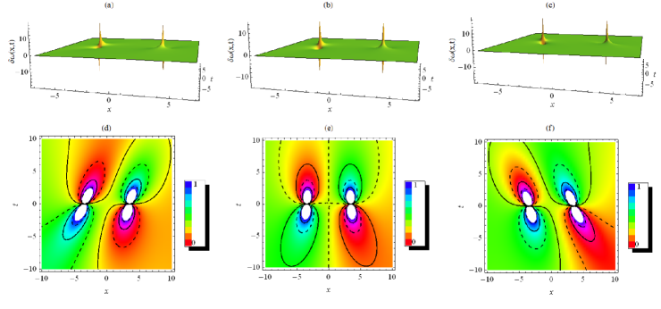
Figure 3: (Color online) 3D (top) and top-view (bottom) distributions of chirp (17b) for the first-order RW solution (17a) with different values of parameter $\beta$. (a,d): $\beta=01/3$; (b,e): $\beta=0$; (c,f): $\beta=1/3$. Other parameters are $r_{0}=0.25$ and $\lambda=0.02$.

III Evolution of chirped rogue waves under the action of the time-dependent atomic scattering length and parabolic potential

In this section, we use the above analytical RW solutions of the cubic GP equation (1) to construct chirped RWs in BEC under the consideration. Throughout this section, without the loss of generality, we take $a_{2}=2$. From the above first- and second-order RW solutions of Eq. (1), we conclude that (i) the amplitude of the chirped RW is proportional to $\sqrt{2a(t)/a_{2}}=\sqrt{a(t)}$, and (ii) chirp $\delta\omega(x,t)$ of the first- and second-order RW is independent of the phase imprint $\theta(x,t)$.

While functions $a(t)$ and $k(t)$ that satisfy the integrability condition (8b) can be arbitrarily chosen to generate the required chirped RW solutions of Eq. (1), in this work we consider either the trap’s frequency $k(t)$ or the Feshbach-managed nonlinearity coefficient $a(t)$ of the following forms: (i) $k(t)=-\lambda^{2}/4$ corresponding to the time-independent expulsive parabolic potential which was used in the creation of bright BEC solitons 8 ; (ii) $a(t)=r_{0}\left[1+m\sin(\omega t)\right]$ with $0<m<1$ and $r_{0}>0$, corresponding to BEC with a time-periodic modulation of the s-wave scattering length 32 ; and (iii) $k(t)=-\left(\mu_{0}^{2}/8\right)\left[1-\tanh\left(\mu_{0}t/2\right)\right]$, where $r_{0}$ is a positive constant 33 . Then, the integrability condition (8b) yields for cases (i), (ii), and (iii) that one should choose, respectively, $a(t)=r_{0}\exp(\lambda t),$ $k(t)=-\left(m\omega^{2}/4\right)\left[m+\sin(\omega t)+m\cos^{2}(\omega t)\right]\left[1+m\sin(\omega t)\right]^{-2}$, and $a(t)=r_{0}\left[1+\tanh\left(\mu_{0}t/2\right)\right]$ with $r_{0}>0$. Note that these forms of the time-dependent trap’s frequency $k(t)$ or FR-managed nonlinearity coefficient $a(t)$ are relevant to BEC experiments 32 ; 33 . Because the amplitude of the above chirped RWs is proportional to $\sqrt{a(t)}$, parameter $r_{0}$ is referred to as the amplitude. In this section, we consider each of the three above-mentioned cases separately, substituting them in the chirped first- and second-order RW solutions (17a) and (19a), and the corresponding expressions for the chirp. Then, we analyze in detail how the chirped RWs get modified by the time-modulation functions $a(t)$ and $k(t)$.

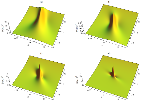
Figure 4: (Color online) The formation of the first-order RWs in BEC with the nonlinearity coefficient exponentially increasing as per Eq. (21) and the time-independent trap’s frequency, $k(t)=-\lambda^{2}/4$. The plots are generated for $\beta=1/3$, $\lambda=0.02$, and different values of the amplitude parameter $r_{0}$ in Eq. (21): $r_{0}=0.05$ (a); $r_{0}=0.1$ (b); $r_{0}=0.15$ (c); $r_{0}=0.3$ (d).

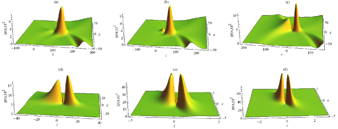
Figure 5: (Color online) Formation of the second-order RWs, in the model with the same $a(t)$ and $k(t)$ as in Fig. 3, the coefficients being $\beta=1/3$ and $\lambda=0.02$. Parameter $r_{0}$ in Eq. ( 21) takes values $r_{0}=0.01$ (a); $r_{0}=0.05$ (b); $r_{0}=0.1$ (c); $r_{0}=0.2$ (d); $r_{0}=0.6$ (e); $r_{0}=1.0$ (f).

III.1 Evolution of chirped rogue waves under the action of the exponentially varying scattering length and expulsive parabolic potential

As the first example, we follow the work of Liang et al. from Ref. 7 and consider BEC with an exponentially varying atomic scattering length in an expulsive (anti-trapping) time-independent harmonic potential, described by Eq. (1) with $k(t)=-\lambda^{2}/4$ and

$$a(t)=r_{0}\exp(\lambda t),$$ (21)

where $r_{0}>0$. Accordingly, we obtain from Eqs. (8a) and (8c) that $\ell(t)=r_{0}^{-1}\exp\left(-\lambda t\right)$ and $T(t)=\left(r_{0}^{2}/2\lambda\right)\left[\exp\left(2\lambda t\right)-1\right]$.

In Fig. 2, the top and bottom panels show, respectively, the 3D and top-view density plots of the first-order RW solution (17a) for different values of $\beta$. When $\beta=0$, Eq. (17a) yields just the standard Peregrine soliton solution to the standard NLS equation 34 , as seen in Figs. 2(b) and (f). These solutions feature one hump and two valleys around the center: the maximum value of the density in the hump is $2.3$, located at $\left(x,t\right)=(0,0)$, and the minimum value in the valleys is $0$, located at $\left(x,t\right)=\left.\left(\pm\sqrt{3}/\left(2r_{0}\right),0\right)\right|_{r_{0}=0.25}\approx\left(\pm 3.4641,0\right)$. When $\beta\neq 0$, it is seen from Figs. 2(a), (b), (c), (d), (g), and (h) that the shape of the first-order RW does not change drastically. However, the three-body interaction term with strength $4\beta^{2}$ and the delayed nonlinear-response one (the last term in Eq. (9)) produce an essential skew angle relative to the ridge of the RW in the anti-clockwise direction for $\beta>0$ (see Figs. 2(g) and (h)), and in the clockwise direction for $\beta<0$, as seen in Figs. 2(d) and (e). As shown by panels (d)-(e) and (g)-(h), the skew angle becomes larger with the increase of $\left|\beta\right|$. From Figs. 2(a), (b), and (c) it is seen that the first-order RW for BEC in the expulsive time-independent parabolic potential are localized in both $x$ and $t$ directions, which means that the first-order RWs can concentrate the condensate in a small region. Unlike classical RWs, plots 2(a), 2(b), and 2(c) show that the nonzero backgrounds of the waves increase with time $t$. This, in turn, means that the dynamics of RWs in BECs with the exponentially varying atomic scattering length in the expulsive time-independent parabolic potential is similar to that in BEC with supply of atoms. This similarity can be conformed by using transformation $\psi(x,t)=\widetilde{\psi}(x,t)\exp\left(-\lambda t/2\right)$.

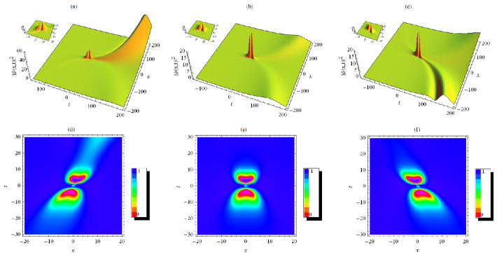
Figure 6: (Color online) Effects of strength $\beta$ of the three-body interaction on the dynamics of the second-order RW in BEC with the exponentially varying atomic scattering length (see Eq. (21) and expulsive time-independent parabolic potential. The top and bottom panels are organized as in Fig. 2, but for the solution given by Eq. (19a), for $\beta=-1/3$ (a,d), $\beta=0$ (b,e), and $\beta=1/3$ (c,f). Parameters $r_{0}$ and $\lambda$, as well as the time-dependent ones, $a(t)$ and $k(t)$, are given in the text.

Figure 3 displays the typical spatiotemporal distribution of chirp $\delta\omega(x,t)$, as given by Eq. (17b), which corresponds to the first-order RW associated with the analytical solution (17a). The figure reveals that the frequency chirp of the first-order RW is localized in both time and space, exhibiting two dark-bright doubly localized structures, with the same location as in the two valleys of the corresponding first-order RW, viz. at $\left(x=\pm\sqrt{3}/\left(2r_{0}\right),0\right)$. Top panels (a), (b), and (c) show that the shape of $\delta\omega(x,t)$ does not change drastically when $\beta\neq 0$ (this is well seen from the comparison of Fig. 3(b) for $\beta=0$ to Figs. 3(a) and 3(c) for $\beta=\pm 1/3$). Nevertheless, the delayed nonlinear response of the system, with coefficient $\beta$, produces, like in Fig. 2, an essential skew angle relative to the ridge of the frequency chirp in the anti-clockwise direction for $\beta>0$ (see Fig. 3(c)), and in the clockwise direction for $\beta<0$, as clearly seen from Fig. 3(a).

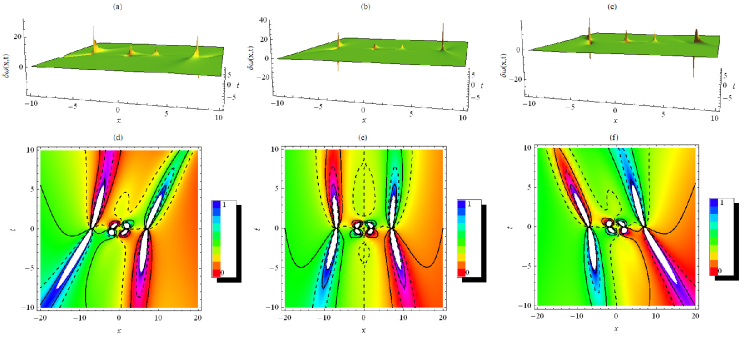
Figure 7: (Color online) 3D (top) and top-view (bottom) distributions of the chirp for the second-order RW solution (19a), given by Eq. (19b), for $k=-\lambda^{2}/4$ and $a(t)$ taken as per Eq. (21), cf. Fig. 3 for the first-order RWs. The results are plotted for $r_{0}=0.25,$ $\lambda=0.02$, and three values of $\beta$, viz., $\beta=-0.7$ (a,d), $\beta=0$ (b,e), and $\beta=0.7.$(c,f).

Now, we aim to demonstrate how the first-order RW in BEC with the exponentially varying atomic scattering length, defined as per Eq. (21), in the time-independent expulsive parabolic potential vary with respect to amplitude parameter $r_{0}$. For this aim, we present in Fig. 4 the formation of the first-order RWs in the cigar-shaped BEC. By varying $r_{0}$ from $0.05$ to $0.3$ in the RW solution (17a), we visualize the formation and manipulation of first-order RWs. When $r_{0}$ smoothly increases, we observe the formation of crests and troughs, as well as an increase of the amplitude and decrease of the width of the isolated wave mode. At $r_{0}=0.3$, a large-amplitude mode is localized in $x$ and $t$, which confirms the formation of the first-order RW. Thus, Fig. 4 reveals that, with the increase of the absolute value of the scattering length through the amplitude parameter $r_{0}$ in Eq. (21), the peak value of the first-order RW grows, and its width compresses. Because the quasi-1D GP equation applies only for low densities, it should be interesting to see how far one can compress the first-order RW in a real experiment, increasing $r_{0}$ as in the above consideration.

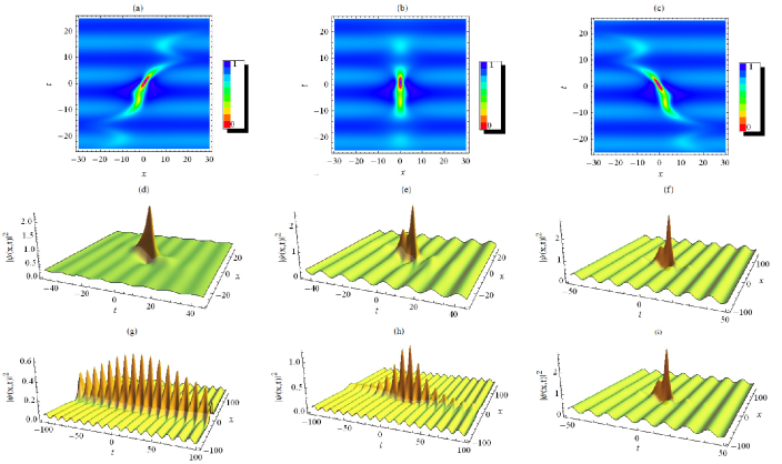
Figure 8: (Color online) Top panels: the density plot for the first-order RW solution (17a) with $r_{0}=0.25,$ $m=0.4$, and for different values of strength $\beta$ of the three-body interaction, viz., $\beta=-0.7$ (a); $\beta=0$ (b); $\beta=0.7$ (c). Middle panels: 3D density plots for the same RW solution with $r_{0}=0.25,$ $\beta=1/3$, and three values of parameter $m$, viz., $m=0.1$ (d); $m=0.4$ (e); $m=0.8$ (f). Bottom panels: density plots for the same RW solution with $\beta=1/3$, $m=0.4$, and three values of the amplitude parameter $r_{0}$, viz., $r_{0}=0.05$ (g), $r_{0}=0.12$ (h); $r_{0}=0.25$ (i). The plots are generated with $\omega=0.5$.

Next, we turn to the consideration of the second-order chirped RW, as per Eq. (19a). It is displayed in Fig. 5, for the time-independent parabolic potential with the atomic scattering length exponentially varying according to Eq. (21). As in the case of the first-order RW, different plots in the figure show that the wave background increases with time $t$. Depending on the value of $r_{0}$ in Eq. (21), the fundamental second-order RW can either remain a single RW (for very small values of $r_{0}$, as seen in Fig. 5(a)), or split into either two first-order RWs, namely, one small-amplitude and one giant RW, as shown in Fig. 5(b), or a set of three first-order RWs, including one small-amplitude and two giant RWs, see Figs. 5(c-f). Thus, Fig. 5 demonstrates the transformation of the second-order RW with the variation of $r_{0}$. At $r_{0}=0.01$, it transforms into the first-order-RW-like structure in Fig. 5(a). When $r_{0}$ increases to $0.05$, a small-amplitude RW (the second RW) emerges, coexisting with a giant RW (the first RW), as seen in Fig. 5(b). When $r_{0}$ increases to some $\widetilde{r}_{0}$, a third RW emerges, coexisting with the first and the second ones, as observed in Fig. 5(c) for $r_{0}=0.1>\widetilde{r}_{0}.$ At all values $r_{0}>\widetilde{r}_{0}$, the three RWs coexist, their amplitudes increasing with the growth of $r_{0}$. This is observed in Figs. 5(d), (e), and (f) for $r_{0}=0.2$, $r_{0}=0.6$, and $r_{0}=1.0$, respectively. As seen in Fig. 5(f), the two giant RWs have almost equal amplitudes for large values of $r_{0}$ (for values slightly exceeding $\widetilde{r}_{0}$, the amplitude of the first RW is larger than that of the third one, as seen in Fig. 5 (d)). For $r_{0}=0.2$ in Fig. 5(d), the first, the second, and third RWs are located, approximately, at $\left(x,y\right)\approx\left(0,5.47\right),$ $\left(0,-6.08\right)$, and $\left(0,-1.16\right)$, respectively, their amplitudes being, respectively, $16.79$, $1.34$, and $13.29$. For $r_{0}=1$ in Fig. 5(f), our calculations show that the maximum amplitude of the first, second, and third RWs are, respectively, $75.80$, $75.102$, and $25$. These maxima are attained, severally, at $\left(x,y\right)\approx\left(0,0.23186\right)$, $\left(0,-0.23289\right)$, and $\left(0,0.00001\right)$. Simultaneously, the width of the modes decreases with the increase of $r_{0}$. Therefore, for BEC with atomic scattering length exponentially varying as per Eq. (21) and the expulsive time-independent parabolic potential, Eq. (19a) can be used to predict the compression of second-order RWs.

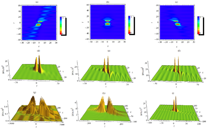
Figure 9: (Color online) Top panels: density plots of the second-order RW solution (19a) with $r_{0}=0.25,$ $m=0.4$, and for different values of strength $\beta$ of the three-body interaction, viz., $\beta=-1/3$ (a); $\beta=0$ (b); $\beta=1/3$ (c). Middle panels: 3D density plots of the same RW solution with $r_{0}=0.25,$ $\beta=1/3$, and three values of parameter $m$, viz., $m=0.1$ (d); $m=0.5$ (e); $m=0.9$ (f). Bottom panels: 3D density plots for the same RW solution for $\beta=1/3$, $m=0.2$, and three values of the amplitude parameter $r_{0}$, viz., $r_{0}=0.01$ (g); $r_{0}=0.05$ (h); $r_{0}=0.25$ (i).

As in the case of the first-order RW, parameter $\beta$ of the three-body interaction does not dramatically affect the shape of the second-order RW, but produces an essential skew angle relative to the RW’s ridge in the anti-clockwise direction for $\beta>0$, and in the clockwise direction for $\beta<0$, cf. Figs. 2 and 3. In Fig. 6 we plot the second-order RW solution (19a) for different values of $\beta$, with $r_{0}=0.25$ and $\lambda=0.02$. Note that each RW in Figs. 6(a), (b), and (c) features three humps, although only the two giant ones are clearly visible. The second-order RW given by Eq. (19a) has four valleys at positions $\left(x,y\right)=\left(x_{0},0\right)$, where $x_{0}=x_{0}(r_{0})$ are real solutions of a cubic equation (with respect to $\left(2r_{0}x\right)^{2}$), $45a_{2}^{3}-90a_{2}^{2}\left(2r_{0}x\right)^{2}-36a_{2}\left(2r_{0}x\right)^{4}+8\left(2r_{0}x\right)^{6}=0$. The minimum value of the solution in the four valleys is $0$. For $r_{0}=0.25$ and $a_{2}=2$, the four valleys are located around the center at positions $\left(x,y\right)\approx\left(-7.028,0\right)$, $\left(-1.859,0\right)$, $\left(1.859,0\right)$, and $\left(7.028,0\right)$.

The frequency chirp $\delta\omega(x,t)$ given by Eq. (19b), which corresponds to the second-order RW solution (19a), is displayed in Fig. 7. This figure reveals that the chirp is localized both in time and space. Furthermore, it exhibits four dark-bright doubly localized structures around $x=0$, located at the same position as the four valleys of the corresponding second-order RW (19a), that is, at $\left(x,y\right)=\left(x_{0}(r_{0}),0\right)$, $x_{0}(r_{0})$ being real solutions of the cubic equation $45a_{2}^{3}-90a_{2}^{2}\left(2r_{0}x\right)^{2}-36a_{2}\left(2r_{0}x\right)^{4}+8\left(2r_{0}x\right)^{6}=0$. As in the case of the first-order RW, the shape of the frequency chirp $\delta\omega(x,t)$ does not dramatically change at $\beta\neq 0$, as seen from comparison of Fig. 7(b), generated for $\beta=0$, with Figs. 7(a) and (c) obtained for $\beta=\pm 0.7$. It is seen in the bottom panels of Fig. 7 that parameter $\beta$ determining the delayed nonlinear response produces, as above, an essential skew angle relative to the ridge of the frequency chirp in the anti-clockwise direction for $\beta>0$, see Fig. 7(c), and in the clockwise direction for $\beta<0$, in Fig. 7(a).

The peaks/holes of the chirp associated to the second-order RW solution (19a) are located at the same position $\left(x_{0},0\right)$ where the corresponding valleys are placed, see the note attached to Eq. (20). For a better presentation of this feature, in Figs. 7(a), (b), and (c) we show the spatiotemporal evolution of the corresponding chirp.

III.2 Evolution of chirped rogues waves under the action of time-periodic modulation of the scattering length

Now, we investigate, as another case of general interest, chirped RWs in the BEC model with a temporally periodic variation of the s-wave scattering length 32 , with

$$a(t)=r_{0}\left[1+m\sin\left(\omega t\right)\right],$$ (22)

where we set $0<m<1$ and $r_{0}>0$. The corresponding potential strength $k(t)$, that satisfies the integrability condition (8b), is taken as

$$k(t)=-\frac{m\omega^{2}\left[m+\sin\left(\omega t\right)+m\cos^{2}\left(\omega t\right)\right]}{4\left[1+m\sin\left(\omega t\right)\right]^{2}}.$$ (23)

Because the amplitude of the chirped RW is proportional to $\sqrt{2a(t)/a_{2}}$, we conclude that the wave’s amplitude will increase with both $r_{0}$ and $m$.

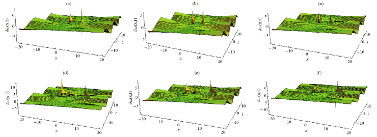
Figure 10: (Color online) Top panels: the distribution of the frequency chirp (17b) corresponding to the first-order RW solution (17a). Bottom panels: the distribution of the frequency chirp (19b) for the second-order RW solution (19a). The plots are generated with $r_{0}=0.25,$ $m=0.4$, $\omega=0.5,$ and three different values of strength $\beta$ of the delayed nonlinear response, viz., $\beta=-1/3$ (a,d); $\beta=0$ (b,e); $\beta=1/3\$(c,f).

For parameters $a(t)$ and $k(t)$ with the time dependence defined as per Eqs. (22) and (23), we display, in Figs. 8, 9, and 10, the first-order RWs, the second-order RWs, and the corresponding chirp, respectively. These figures show that, due to the periodic modulation, the first- and second-order RWs, as well as the corresponding chirp propagate on top of the modulated CW background. For $\beta=-1/3$, the first- and second-order RWs are shown, respectively, in Figs. 8(a) and 9(a). For $\beta=0$, RWs of the same types are displayed in Figs. 8(b) and 9(b), respectively. Finally, for $\beta=1/3$, the solutions are presented in Figs. 8(c) and 9(c). From these figures, one can conclude that the three-body interaction with strength $\beta$ produces, as above, an essential skew angle relative to the ridge of the RW, in the clockwise direction for $\beta<0$, and in the anti-clockwise direction for $\beta>0$. For different values of parameters $m$ and $r_{0}$ in Eq. (22) $a(t)$, we plot, severally, in the middle and bottom panels of Figs. 8 and 9 the first-order RW solution given by Eq. (17a), and the second-order RW solution (19a). These plots demonstrate how parameters $m$ and $r_{0}$ affect the amplitude and structure of the first- and second-order RWs. In particular, the modes’ amplitudes increase as $m$ and $r_{0}$ grow. It is seen from the plots in the middle panels that the best structure of the first- and second-order RWs is obtained for small values of $m$, see Figs. 8(d) and 9(d). Further, the bottom panels in Figs. 8 and 9 reveal that the best structure of the RWs is attained for higher values of $r_{0}$, see Fig. 8(i) and 9(i). Therefore, parameters $m$ and $r_{0}$ in Eq. (22) have the same effect on the waves’ amplitudes and opposite effect on their structure, in the sense that the best structure is achieved either by decreasing $m$ or increasing $r_{0}$. Figure 8(g) also demonstrates that, for small values of $r_{0}$, the first-order RW behaves like a breather soliton propagating on top of a modulated CW background.

The top and bottom panels of Fig. 10 showing the distribution of the frequency chirp which corresponds, respectively, to the first- and second-order RWs, it is clearly seen that, under the action of the time-periodic modulation of the s-wave scattering length, the chirp is localized in time and space on top of the CW background. Further, the top and bottom panels in the figure reveal that the chirp corresponding, respectively, to the first- and second-order RWs exhibit two- and four-peak dark-bright doubly localized structures, located (as above) at the same positions where valleys of the corresponding RWs are found. The plots related to different signs ($-$, $0$, or $+$) of coefficient $\beta$ of the delayed nonlinear response in the system do not strongly affect the shape of the RWs. Nevertheless, also similar to what was observed in several patterns displayed above, $\beta$ determines an essential skew angle relative to the ridge of the chirp in the counter-clockwise direction for $\beta>0$, and in the clockwise direction for $\beta<0$ (in the present case, this feature, typical for all the RW patterns considered in this work, is not shown in detail).

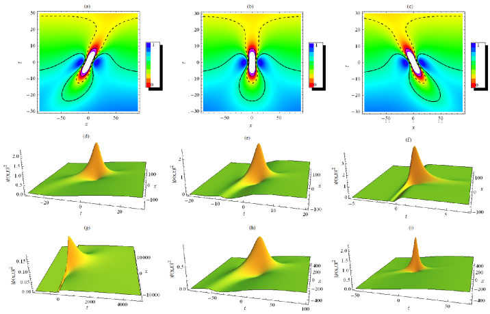
Figure 11: (Color online) Density plots for the first-order RW solution (17a) of Eq. (1) with the time-modulation format given by Eqs. (24) and (25). Top panels: the plots for $r_{0}=0.25,$ $\mu_{0}=0.05$, and different values of strength $\beta$ of the three-body interaction, viz., $\beta=-1/3$ (a); $\beta=0$ (b); $\beta=1/3$ (c). Middle panels: the plots for $r_{0}=0.25,$ $\beta=-1/3$, and three values of $\mu_{0}$, viz., $\mu_{0}=0.1$ (d); $\mu_{0}=0.4$ (e); $\mu_{0}=5$ (f). Bottom panels: the plots for $\beta=-1/3$, $\mu_{0}=0.05$, and three values of the $r_{0}$, viz., $r_{0}=0.05$ (g), $r_{0}=0.1$ (h); $r_{0}=0.25$ (i).

III.3 Chirped rogue waves in under the action of the scattering length and expulsive parabolic potential subjected to the stepwise temporal modulation

As the third example, we consider chirped RWs controlled by a time-dependent scattering length combined with the expulsive parabolic potential whose strength, $k(t)$, vanishes at $t\rightarrow\infty$. Following Ref. 33 ; 34 , we choose a stepwise modulation profile satisfying this condition:

$$k(t)=-\frac{\mu_{0}^{2}}{8}\left[1-\tanh\left(\frac{\mu_{0}}{2}t\right)\right],$$ (24)

with $\mu_{0}>0$. Substituting this in integrability condition (8b), we find the respective time-modulation form of the nonlinearity coefficient,

$$a(t)=r_{0}\left[1+\tanh\left(\frac{\mu_{0}}{2}t\right)\right],$$ (25)

where $r_{0}$ is an arbitrary positive constant. Because the amplitude of the first- and second-order chirped RWs, given by Eqs. (17a) and (19a), is proportional to $\sqrt{2a(t)/a_{2}}=\sqrt{r_{0}\left[1+\tanh\left(\mu_{0}t/2\right)\right]}$, we conclude that the waves’ amplitudes increase with the growth of $r_{0}$ and $\mu_{0}$.

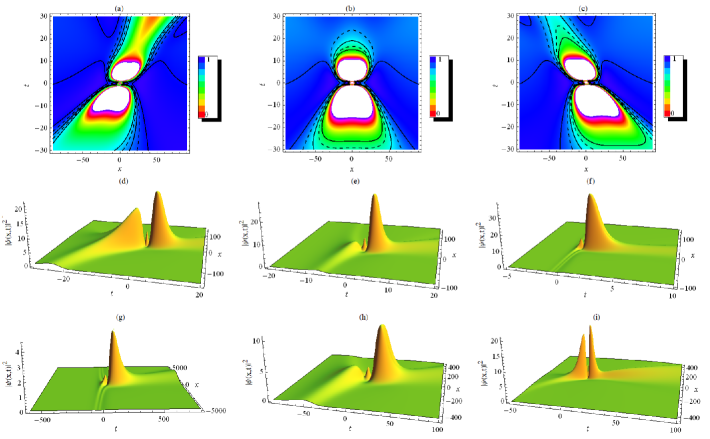
Figure 12: (Color online) Density plots for the second-order RW solution (19a) with the time-modulation format, defined by Eqs. ( 24) and (25). Top panels: the plots for $r_{0}=0.25,$ $\mu_{0}=0.05$, and different values of strength $\beta$ of the three-body interaction, viz., $\beta=-1/3$ (a); $\beta=0$ (b); $\beta=1/3$ (c). Middle panels: the plots for $r_{0}=0.25,$ $\beta=-1/3$, and different values of $\mu_{0}$, viz., $\mu_{0}=0.1$ (d); $\mu_{0}=0.4$ (e); $\mu_{0}=5$ (f). Bottom panels: the plots for $\beta=-1/3$, $\mu_{0}=0.05$, and three values of $r_{0}$, viz., $r_{0}=0.03$ (g), $r_{0}=0.1$ (h); $r_{0}=0.25$ (i).

To present effects of modulation parameters $r_{0}$ and $\mu_{0}$ in Eqs. (24) and (25) on the chirped first- and second-order RWs, in Figs. 11, 12, and 13 we display the first-order RW given by Eq. (17a), the second-order RW given by Eq. (19a), and the first- and second-order chirped RWs produced by Eqs. (17b) and (19b), respectively. In Figs. 11 and 12, the RWs (17a) and (19a) with $\beta=0$ reduce to the standard Peregrine soliton and the standard second-order RW solution of the integrable NLS equation, see Figs. 11(a) and 12(a). Further, the middle and bottom panels of Figs. 11 and 12 reveal that, under the action of the temporal modulation defined by Eqs. (24) and (25), the first- and second-order RWs given by Eqs. (17a) and (19a) propagate on top of a kink-shaped background. It is also seen in the top panels of Figs. 11 and 12 that quintic coefficient $\beta$ from Eq. (9) produces, similar to what was seen in the above solutions, an essential skew angle relative to the ridge of the RW in the clockwise direction for $\beta>0$ (Figs. 11(a) and 12 (a)), and in the anti-clockwise direction for $\beta>0$ (Figs. 11(c) and 12(c)). As $\left|\beta\right|$ gets larger, the skew angle becomes larger too (not shown here in detail). It is seen in the middle and bottom panels of Fig. 12 that the first-order RW, given by Eq. (17a), with the modulation format (24) and (25), is composed of one hump and two valleys located around the center: the amplitude of the hump is $18r_{0}/a_{2}=9r_{0}$, attained at $(x,y)=\left(0,0\right)$, while the minima in the valleys is $0$, located at $\left(x,y\right)=\left(\pm\sqrt{3}/\left(2r_{0}\right),0\right)$. Obviously, $\left(\pm\sqrt{3}/\left(2r_{0}\right),0\right)\rightarrow\left(0,0\right)$ as $r_{0}\rightarrow+\infty$, meaning that, for large $r_{0}$, the first-order RW contains a single hump, as seen in Fig. 11(f), plotted for $r_{0}=5$. Also, $\left(\pm\sqrt{3}/\left(2r_{0}\right),0\right)\rightarrow\left(\pm\infty,0\right)$ at $r_{0}\rightarrow+0$, hence the two valleys of the first-order RW escape to infinity; in this case, the first-order RW also contains one hump, as seen in Fig. 11(g), plotted for $r_{0}=0.01$. The middle and bottom panels of Fig. 11, obtained for different values of, respectively, parameters $\mu_{0}$ and $r_{0}$, show that the amplitude of the first-order RW, given by Eq. (17a), increases with each of these two parameters. These panels of Fig. 11 also show that the mode’s width decreases with the increase of $\mu_{0}$ and $r_{0}$. Therefore, these parameters can be used to control both the amplitude and width of the first-order RW corresponding to the modulation format based on Eqs. (24) and (25). The middle and bottom panels of Fig. 12 show that the best structure of the first-order RW, composed of the single hump and two valleys, is obtained with small values of $\mu_{0}$ (see Fig. 11(d)) and large values of $r_{0}$ (see Fig. 11 (f)).

Figure 13: (Color online) The distribution of the frequency chirp (17b) associated with the first-order RW solution (17a) (top), and frequency chirp (19b) corresponding to the second-order RW solution (19a) (bottom). The step-like modulation format is taken as per Eqs. (24) and (25). The plots are generated for $r_{0}=0.25$, $\mu_{0}=0.1$, and three different values of strength $\beta$ of the delayed nonlinear response, viz., $\beta=-0.7$ (a,d);: $\beta=0$, (b,c) and $\beta=0.7$ (e,f).

The middle and the bottom panels of Fig. 12 displays the second-order RW solution (19a) at different values of, respectively, $\mu_{0}$ and $r_{0}$. These plots show how parameters $\mu_{0}$ and $r_{0}$ from Eqs. (24) and (25) affect the structure of the second-order RWs. It is seen that, for small values of $\mu_{0}$ (see the middle panels) or large values of parameter $r_{0}$ (in the bottom panels), the second-order RW features three humps — namely, from right to left, the main (giant) hump, a dwarf one, and a secondary hump. The middle (bottom) panel in Fig. 12 reveals that the amplitude of the secondary hump decreases as parameter $\mu_{0}$ increases ($r_{0}$ decreases), and thus the hump disappears at a critical value of $\mu_{0}$ ($r_{0}$). It is also seen from Figs. 12(d), (e), and (f) that the amplitudes of the giant and dwarf humps increase, and their widths decrease, with the growth of both $\mu_{0}$ and $r_{0}$. From the middle and bottom panels of Fig. 12 we conclude that, for small values of $\mu_{0}$, while $r_{0}$ is kept fixed, or for large values of $r_{0}$, while $\mu_{0}$ is kept constant, the second-order RW is built of a dwarf hump, one secondary and one giant ones, and four valleys around the center, as seen from Figs. 12(d) and 12(i). The minimum in the four valleys is $0$, located approximately at $\left(\pm 1.860/r_{0},0\right)$ and $\left(\pm 7.028r_{0}^{-1},0\right)$. As these points approach $\left(x,y\right)=\left(0,0\right)$ at $r_{0}\rightarrow+\infty$, at large values of $r_{0}$ the three humps fuse to form a single giant one, while the four valleys disappear. We also note that, as the same points move to $\left(\pm\infty,0\right)$ at $r_{0}\rightarrow+0$, the second-order RW keeps a single giant hump at $r_{0}$ small enough, and this RW seems like a first-order one.

Figure 13 displays, for $r_{0}=0.25$, $\mu_{0}=0.1$, and three different values of $\beta$, the distribution of the frequency chirp, given by Eq. (17b), for the first-order RW solution (17a) (top panels), and the chirp, given by Eq. (19b), for the second-order RW solution (19a) (bottom panels). As in the two examples considered above, the chirp associated with the first-order and the second-order RWs is localized in time and space, and exhibits, respectively, two and four dark-bright localized structures. Although strength $\beta$ of the delayed nonlinear response does not strongly affect the shape of the frequency chirp, it produces, as in the solutions considered above, an essential skew angle relative to the ridge of the chirp in the anti-clockwise direction for $\beta>0$, and in the clockwise direction for $\beta<0$, as is clearly seen in Fig. 13.

IV Conclusion

We have studied the generation of first- and second-order chirped RWs (rogue waves) in the BEC model with the time-varying atomic scattering length in the expulsive parabolic potential. The model is based on the cubic GP equation (1) for the mean-field wave function. By combining the modified lens-type transformation with the phase engineering technique, the cubic GP equation was transformed into the Kundu-Eckhaus equation with the quintic nonlinearity and the term which represents the Raman effect in fiber optics. We considered solutions based on the CW background which satisfies condition (14) of the baseband modulational instability. The resulting equation is integrable if strength $k(t)$ of the parabolic potential and nonlinearity strength $a(t)$ satisfy integrability condition (8b). Using the known first- and second-order RW solutions of the KE equation, we have presented explicit first- and second-order chirped RW solutions (17a) and (19a), along with the corresponding expressions (17b) and (19b) for the local chirp. Then, we have identified the first- and second-order chirped RWs in the model with (i) the exponentially time-varying atomic scattering length (Eq. (21)), (ii) time-periodic modulation of the nonlinearity, and (iii) the stepwise temporal modulation based on Eqs. (24) and (25). In each case, the effects produced by strength $\beta$ of the delayed nonlinear response on the chirped RWs are analyzed. This parameter affects the spatial location of the humps in the first- and second-order RWs, whereas the amplitudes of the humps and the time of their appearance remain unaltered. More interestingly, we have found that the first-order (second-order) RWs involve a frequency chirp that is localized in time and space. Moreover, we have found that the chirp of the first- and second-order RW exhibits, respectively, two or four dark-bright localized structures.

We have also studied in detail characteristics of the constructed RWs in terms of the time-dependent parameters $a(t)$ and $k(t)$. The results demonstrate how these parameters affect the first- and second-order RWs. It is shown that they can be used to manage the evolution of the RWs. We have also observed that the behavior of the RW’s background changes, depending on the temporal modulation of $a(t)$ and $k(t)$. The results of this work suggest possibilities to manipulate RWs experimentally in BEC with the atomic scattering length modulated in time by means of the FR (the Feshbach resonance).

Compliance with ethical standards

Conflict of interest: The authors declare that they have no conflict of interest.

References

- (1) S. Burger, K. Bongs, S. Dettmer, W. Ertmer, K. Sengstock, A. Sanpera, G. V. Shlyapnikov, and M. Lewenstein, Phys. Rev. Lett. 83, 5198 (1999); J. Denschlag, J.E. Simsarian, D.L. Feder, Charles W. Clark, L.A. Collins, J. Cubizolles, L. Deng, E.W. Hagley, K. Helmerson, W.P. Reinhardt, S.L. Rolston, B.I. Schneider, W.D. Phillips, Science 287, 97 (2000); Th. Busch and J. R. Anglin, Phys. Rev. Lett. 84, 2298 (2000); C.K. Law, C.M. Chan, P.T. Leung, and M.-C. Chu, Phys. Rev. Lett. 85, 1598 (2000).
- (2) B.P. Anderson, P.C. Haljan, C.A. Regal, D.L. Feder, L.A. Collins, C.W. Clark, and E.A. Cornell, Phys. Rev. Lett. 86, 2926 (2001); B.P. Anderson, Dark Solitons in BECs: The first experiments. In: Kevrekidis P.G., Frantzeskakis D.J., Carretero-González R. (eds) Emergent Nonlinear Phenomena in Bose-Einstein Condensates. Atomic, Optical, and Plasma Physics, vol 45. Springer, Berlin, Heidelberg; T. Bland, K. Pawłowski, M.J. Edmonds, K. Rzazewski, and N.G. Parker, Phys. Rev. W A 95, 063622 (2017); Th. Busch and J. R. Anglin, Phys. Rev. Lett. 84, 2298 (2000).
- (3) W.-M. Liu and E. Kengne, Schrödinger Equations in Nonlinear Systems. Springer Nature Singapore Pte Ltd. (2019); E. Kengne, A. Sheou, and A. Lakhssassi, Eur. Phys. J. B 89, 1 (2016).
- (4) D. L. Wang et al., Chin. Phys. Lett. 24, 1817 (2002); E. Kengne and W.-M. Liu, Phys. Rev. E 98, 012204 (2018); F. D. Zong and J. F. Zhang, ibid. 25, 2370 (2008). Z. X. Liang, Z. D. Zhang, and W.-M. Liu, Phys. Rev. Lett. 94, 050402 (2005).
- (5) K. E. Strecker, G. B. Partridge, A. G. Truscott, and R. G. Hulet, Nature 417, 150 (2002); L. Khaykovich, F. Schreck, G. Ferrari, T. Bourdel, J. Cubizolles, L. D. Carr, Y. Castin, and C. Salomon, Science 296, 1290 (2002); P.G. Kevrekidis, G. Theocharis, D.J. Frantzeskakis, and B. A. Malomed, Phys. Rev. Lett. 90, 230401 (2003); E. Kengne and A. Lakhssassi, Inter. J. Mod. Phys. B 32, 1850184 (2018); E. Kengne and W.-M. Liu, J. Phys. B: At. Mol. Opt. Phys. 53, 215003 (2020); E. Kengne and A. Lakhssassi, Nonlinear Dyn. 104, 4221 (2021).
- (6) A. Di Carli, C. D. Colquhoun, G. Henderson, S. Flannigan, G. L. Oppo, A. J. Daley, S. Kuhr, and E. Haller, Phys. Rev. Lett. 123, 123602 (2019).
- (7) O. V. Marchukov, B. A. Malomed, M. Olshanii, J. Ruhl, V. Dunjko, R. G. Hulet, and V. A. Yurovsky, Phys. Rev. Lett. 125, 050405 (2020); D. Luo, Y. Jin, J. H. V. Nguyen, B. A. Malomed, O. V. Marchukov, V. A. Yurovsky, V. Dunjko, M. Olshanii, and R. G. Hulet, Phys. Rev. Lett. 125, 183902 (2020).
- (8) E. Kengne, Eur. Phys. J. Plus 135, 622 (2020); E. Kengne, A. Lakhssassi, and W.-M. Liu, Nonlinear Dynamics 97, 449 (2019); W.-R. Sun and L. Wang, Proc. R. Soc. A. 474, 20170276 (2018).
- (9) L. Wen, L. Li, Z. D. Li, S. W. Song, X. F. Zhang, and W.-M. Liu, Eur. Phys. J. D 64, 473(2011); Wen-Rong Sun, Bo Tian, Yan Jiang,a nd Hui-Ling Zhen, Eur. Phys. J. D 68, 282 (2014); L. Li, and F. Yu, Sci Rep 7, 10638 (2017).
- (10) B. Eiermann, T. Anker, M. Albiez, M. Taglieber, P. Treutlein, K. P. Marzlin, and M. K. Oberthaler, Phys. Rev. Lett. 92, 230401 (2004); Xing Zhua, Huagang Li, and Zhiwei Shi, Phys. Lett. A 23, 3253 (2016); L. Zeng and J. Zeng, Advanced Photonics 1, 046004 (2019); V. Delgado and A. Muñoz Mateo, Sci. Rep. 8, 10940 (2018); R. Ravisankar, T. Sriraman, L. Salasnich, and P. Muruganandam, J. Phys. B: At. Mol. Opt. Phys. 19, 195301 (2020).
- (11) O. Morsch and M. Oberthaler, Rev. Mod. Phys. 78, 179-215 (2006).
- (12) M. R. Matthews, B. P. Anderson, P. C. Haljan, D. S. Hall, C. E. Wieman, and E. A. Cornell, Phys. Rev. Lett. 83 , 2498 (1999); N. V. Hung, P. Szańkowski, V. V. Konotop, and M. Trippenbach, J. Phys. B: At. Mol. Opt. Phys. 22, 053019 (2020); J. P. Burke Jr, P. S. Julienne, C. J. Williams, Y. B. Band, M. Trippenbach, arXiv.org cond-mat, arXiv:cond-mat/0404499; O. Danaci, C. Rios, and R. T. Glasser, Proceedings 9950, Laser Beam Shaping XVII, 99500D (2016).
- (13) D. S. Petrov, Phys. Rev. Lett. 115, 155302 (2015); D. S. Petrov and G. E. Astrakharchik, Phys. Rev. Lett. 117, 100401 (2016); M. Tylutki, G. E. Astrakharchik, B. A. Malomed, and D. S. Petrov, Phys. Rev. A 101, 051601(R) (2020).
- (14) C. R. Cabrera, L. Tanzi, J. Sanz, B. Naylor, P. Thomas, P. Cheiney, and L. Tarruell, cience 359, 301 (2018); P. Cheiney, C. R. Cabrera, J. Sanz, B. Naylor, L. Tanzi, and L. Tarruell, Bright soliton to quantum droplet transition in a mixture of Bose-Einstein condensates, Phys. Rev. Lett. 120, 135301 (2018); G. Semeghini, G. Ferioli, L. Masi, C. Mazzinghi, L. Wolswijk, F. Minardi, M. Modugno, G. Modugno, M. Inguscio, and M. Fattori, Self-bound quantum droplets in atomic mixtures, Phys. Rev. Lett. 120, 235301 (2018); G. Ferioli, G. Semeghini, L. Masi, G. Giusti, G. Modugno, M. Inguscio, A. Gallemí, A. Recati, and M. Fattori, 122, 090401 (2019); C. D’ Errico, A. Burchianti, M. Prevedelli, L. Salasnich, F. Ancilotto, M. Modugno, F. Minardi, and C. Fort, Phys. Rev. Research 1, 033155 (2019).
- (15) I. Ferrier-Barbut, H. Kadau, M. Schmitt, M. Wenzel, and T. Pfau, Observation of quantum droplets in a strongly dipolar Bose gas, Phys. Rev. Lett. 116, 215301 (2016); L. Chomaz, S. Baier, D. Petter, M. J. Mark, F. Wächtler, L. Santos, and F. Ferlaino, Phys. Rev. X 6, 041039 (2016).
- (16) V. E. Zakharov, S. V. Manakov, S. P. Novikov, and L. P. Pitaevskii, Solitons: Inverse Scattering Method (Nauka publishers, Moscow, 1980; English translation: Consultants Bureau, New York, 1984).
- (17) M. J. Ablowitz and P. A. Clarkson, Solitons, Nonlinear Evolution Equations and Inverse Scattering (Cambridge University Press, New York, 1991).
- (18) J. P. Ying, Commun. Theor. Phys. 35, 405 (2001); C. Bai and H. Zhao, Eur. Phys. J. D 39, 93 (2006); S. Wang, X. Y. Tang, and S. Y. Lou, Chaos, Solitons & Fractals, 21, 231 (2004); Yu-Lan Ma and Bang-Qing Li, AIMS Mathematics 5, 1162 (2020).
- (19) J. F. Zhang, G. P. Guo, and F. M. Wu, Chin. Phys. 12, 533 (2002); A. Ankiewicz and A. Chowdury, Zeitschrift für Naturforschung A 71, 647 (2016); J. Lin, Y. S. Xu, F. M. Wu, Chin. Phys. 12, 1049 (2003); W. Rui and Y. Zhang, Adv. Differ. Equ. 2020, 195 (2020).
- (20) E. Kengne, W.-M. Liu, and B.A. Malomed, Spatiotemporal engineering of matter-wave solitons in Bose-Einstein condensates. Phys. Rep. 899, 1-62 (2021).
- (21) Yu. V. Bludov, V. V. Konotop, and N. Akhmediev, Phys, Rev. A 80, 033610 (2009).
- (22) S. Chen, F. Baronio, J.M. Soto-Crespo, P. Grelu, and D. Mihalache, J. Phys. A: Math. Theor. 50 463001 (2017).
- (23) B. Kibler, A. Chabchoub, A. Gelash, N. Akhmediev and V.E. Zakharov, Phys. Rev. X 5, 041026 (2015).
- (24) J.M. Dudley, G. Genty, F. Dias, B. Kibler, and N. Akhmediev, Opt. Express 17, 21497 (2009); E. Kengne, Chaos, Solitons & Fractals 146, 110866 (2021).
- (25) K. Manikandan, P. Muruganandam, M. Senthilvelan, and M. Lakshmanan, Phys. Rev. E 90, 062905 (2014); A.R. Osborne, Nonlinear Ocean waves (Academic Press, New York, 2009).
- (26) Yu. V. Bludov, V. V. Konotop, and N. Akhmediev, Phys, Rev. A 80, 033610 (2009).
- (27) N. Akhmediev, A. Ankiewicz, and J. M. Soto-Crespo, Phys. Rev. E 80, 026601 (2009); ] N. Akhmediev, A. Ankiewicz, and M. Taki, Phys. Lett. A 373, 675 (2009); E. Kengne and W. M. Liu, Phys. Rev. E 102, 012203 (2020); D. H. Pergrine, J. Austral. Math. Soc. Ser. B 25, 16 (1983).
- (28) A. Gammal, T. Frederico, L. Tomio, and Ph. Chomaz, J. Phys. B 33, 4053 (2000).
- (29) V. R. Kumar, R. Radha, and M. Wadati, J. Phys. Soc. Jap. 79, 074005 (2010); E. Kengne, A. Lakhssassi, W.-M. Liu, and R. Vaillancourt, Phys. Rev. E 87, 022914 (2013); E. Kengne and W.-M. Liu, Phys. Rev. E 102, 012203 (2020); E. Kengne and W. M. Liu, Adv. Theory Simul. 2021, 2100062 (2021).
- (30) F. K. Abdullaev, A. Gammal, L. Tomio, and T. Frederico, Phys. Rev. A 63, 043604 (2001).
- (31) G. P. Agrawal, Nonlinear Fiber Optics, 4th ed. (Academic Press, 2007); Yu. S. Kivshar and G. P. Agrawal, Optical Solitons: From Fibers to Photonic Crystals (Academic, 2003).
- (32) A.S. Reyna and C.B. de Araújo, Adv. Opt. Phot. 9, 720 (2017).
- (33) B. A. Malomed, Soliton Management in Periodic Systems (Springer, New York, 2006).
- (34) J. Cuevas, P. G. Kevrekidis, B. A. Malomed, P. Dyke, and R. G. Hulet, New J. Phys. 15, 063006 (2013).
- (35) V.M. Perez-Garcia, H. Michinel, and H. Herrero, Phys. Rev. A 57, 3837 (1998); U. Al. Khawaja, J. Phys. A 39, 9679 (2006); E. Kengne and P. K. Talla, J. Phys. B 39, 3679 (2006); A. Mohamadou,. E. Wamba, S. Y. Doka, T.B. Ekogo, and T. C. Kofane, Phys. Rev. A 84, 023602 (2011).
- (36) V. I. Kruglov, A. C. Peacock, and J. D. Harvey, Phys. Rev. Lett. 90, 113902 (2003); M. Desaix, L. Helczynski, D. Anderson, and M. Lisak, Phys. Rev. E 65, 056602 (2002); H. Triki, Anjan Biswas, D. Milović, and M. Beliće, Optics Communications 366, 362 (2016); A. A. Goyal, R. Gupta, and C. N. Kumar, Phys. Rev. A 84, 063830 (2011); K. Senthilnathan, K. Nakkeeran, Q. Li and P. K. A. Wai, 2009 14th OptoElectronics and Communications Conference, Vienna, 2009, pp. 1-2, doi: 10.1109/OECC.2009.5214444; H. Kumar and F Chand, Journal of Nonlinear Optical Physics & Materials 22, 1350001 (2013).
- (37) L. V. Hmurcik and D. J. Kaup, J. Opt. Soc. Am. 69, 597 (1979); T. Kaczmarek, Optica Applicata 34, 241 (2004); I. Babushkin, S. Amiranashvili, C. Brée, U. Morgner, G. Steinmeyer, and A. Demircan, IEEE Photonics Journal Effect of Chirp on Pulse Compression 8, 7803113 (2016).
- (38) K. Senthilnathan, Qian Li, P.K.A. Wai, and K. Nakkeeran, PIERS Online 3, 531 (2007); A. Bouzidaa, H. Triki, M. Z. Ullahb, Q. Zhouc, A. Biswas, and M. Belic, Optik 142, 77 (2017); E. Kengne and R. Vaillancourt, Can. J. Phys. 87, 1191 (2009).
- (39) S. Chen, Y. Zhou, L. Bu, F. Baronio, J. M. Soto-Crespo, and D. Mihalache, Optics Express 27, 11370 (2019).
- (40) L. F. Mouassom, A. Mvogo, and C.B. Mbane, Pramana - J Phys 94, 10 (2020).
- (41) F.-D. Zong, Yang Yang, and J.-F. Zhang, Acta Physica Sinica -Chinese Edition- 58, 3670 (2009); Zhenyun Qina and Gui Mu, Zeitschrift für Naturforschung A 67, 141 (2012); U. Al Khawaja, J. Phys. A: Math. Theor. 42, 265206 (2009); Heping Jia, Rongcao Yang, Chaoqing Dai, and Yanyan Guo, Journal of Modern Optics 66, 665 (2019).
- (42) A. Kundu, J. Math. Phys. 25, 3433 (1984); F. Calogero and W. Eckhaus, Inverse Probl. 3, 229 (1987).
- (43) R. S. Johnson, Proc. R. Soc. London A 357, 131 (1977); Y. Kodama, J. Stat. Phys. 39, 597 (1985); P. A. Clarkson and J. A. Tuszynski, J. Phys. A 23, 4269 (1990); D. Qiu, J. He, Y. Zhang and K. Porsezian, Proc. R. Soc. A. 471, 0236 (2015); A. Bekir and E. H. M. Zahran, Optik 223, 165233 (2020).
- (44) P. A. Clarkson and C. M. Cosgrove, J. Phys. A Math. Gen. 20, 2003 (1987).
- (45) S. Burger, K. Bongs, S. Dettmer, W. Ertmer, K. Sengstock, A. Sanpera, G. V. Shlyapnikov, and M. Lewenstein: Phys. Rev. Lett. 83, 5198 (1999).
- (46) X. Wang, B. Yang, Y. Chen, and Y. Yang, Phys. Scr. 89, 095210 (2014).
- (47) E. Kengne and W.-M. Liu, Phys. Rev. E 99, 062222 (2019); E. Kengne and W.-M. Liu, Phys. Rev. E 73, 026603 (2006).
- (48) A. Mohamadou, E. Wamba, S.Y. Doka, T.B. Ekogo, and T.C. Kofané, Phys. Rev. A 84, 023602 (2011); E. Kengne, C. Tadmon, and R. Vaillancourt, Chin. J. Phys. 47, 80 (2011).
- (49) F. Baronio, S. Chen, Ph. Grelu, S. Wabnitz, and M. Conforti, Phys. Rev. A 91, 033804 (2015); F. Baronio, M. Conforti, A. Degasperis, S. Lombardo, M. Onorato, and S. Wabnitz, Phys. Rev. Lett. 113, 034101 (2014).
- (50) H. Saito and M. Ueda, Phys. Rev. Lett. 90, 040403 (2003); G.S Chong, H. HaiW and Q.T Xie, Chin. Phys. Lett. 20, 2098 (2003).
- (51) S. Rajendran, P. Muruganandam, and M. Lakshmanan, Physica D 239, 366 (2010).
- (52) D. H. Peregrine, J. Austral, Math. Soc. B: Appl. Math. 25, 16 (1983).