Abstract

The tadpole conjecture by Bena, Blåbäck, Graña and Lüst effectively states that for string-theory compactifications with a large number of complex-structure moduli, not all of these moduli can be stabilized by fluxes. In this note we study this conjecture in the large complex-structure regime using statistical data obtained by Demirtas, Long, McAllister and Stillman for the Kreuzer-Skarke list. We estimate a lower bound on the flux number in type IIB Calabi-Yau orientifold compactifications at large complex-structure and for large $h^{2,1}$, and our results support the tadpole conjecture in this regime.

1 Introduction

String theory is a consistent theory in ten flat space-time dimensions. Its five known formulations are related to each other by various dualities, and hence the theory is essentially unique. However, when compactifying string theory to lower dimensions one obtains an abundance of effective theories known as the string-theory landscape. Famous estimates for the size of this landscape are $10^{500}$, $10^{930}$, $10^{1500}$ and $10^{272000}$, which have appeared in [1, 2, 3, 4]. But, although the landscape is vastly large, typically not all solutions are of interest to us. For instance, one often restricts one’s attention to effective four-dimensional theories with few or no massless scalar fields. For the type II string such theories can be obtained by compactifying on Calabi-Yau three-folds in the presence of fluxes, where the choice of fluxes is constrained by the tadpole cancellation condition (for a review see for instance [5]). Remarkably, using this tadpole condition it has been argued that for a given compactification manifold the number of flux vacua is finite [6, 7].

Let us become a bit more concrete: compactifications of string theory on Calabi-Yau manifolds without fluxes typically lead to a large number of massless scalar fields (moduli) in the effective theory. By turning on fluxes these can be stabilized and one would expect that for a generic choice of fluxes all moduli can be stabilized in a suitable regime. This is an underlying assumption in the KKLT [8] and Large-Volume (LVS) [9] scenarios. However, this expectation may be too naive. Indeed, in [10] it has been argued that to stabilize moduli near a certain conifold locus, large fluxes have to be considered which are not compatible with the tadpole cancellation condition. In [11] we discussed that the tadpole cancellation condition can force moduli to be stabilized in a perturbatively poorly-controlled regime, and in [12] the authors show that for M-theory compactifications stabilizing all moduli can be in tension with the tadpole condition. Thus, the landscape of four-dimensional effective theories with no or few massless scalar fields may be smaller than expected.

In [13] this observation has been formulated as the tadpole conjecture, and further evidence has been provided in [14]. Several versions of this conjecture have been stated, and in this note we are interested in the type IIB version with respect to the complex-structure moduli. With $N_{\rm flux}$ denoting the flux number encoding the contribution of the Neveu-Schwarz–Neveu-Schwarz (NS-NS) and Ramond-Ramond (R-R) three-form fluxes to the D3-brane tadpole condition, it states that

$$\begin{split}N_{\rm flux}>2\hskip 1.0pt\alpha\hskip 1.0pt(h^{2,1}+1)\hskip 50.0pt\mbox{for}\quad h^{2,1}\gg 1\,,\end{split}$$ (1.1)

where $h^{2,1}$ counts the number of complex-structure moduli and the constant $\alpha$ has been conjectured to be $\alpha=1/3$. For relevant examples this bound is indeed satisfied (see for instance table 1.1 in [13]). If the tadpole conjecture is true, then in the large $h^{2,1}$ limit the contribution of fluxes to the tadpole cancellation condition cannot be cancelled by orientifold planes, and hence it is not possible to stabilize all moduli consistently. This would violate a common assumption of the KKLT and LVS constructions for large $h^{2,1}$. We mention however that in [15] a scenario evading the bound (1.1) has been proposed, which is currently under debate.

The tadpole conjecture has important implications for the string-theory landscape, but finding a proof appears to be difficult. In this note we give an explanation for why it is difficult to prove this conjecture, and we present arguments in its favor in the large complex-structure limit. More concretely,

• in section 2 we briefly recall some aspects of moduli stabilization for type IIB orientifolds in the presence of fluxes. This section contains no new results and can be skipped by the reader familiar with the topic.

• In section 3 we argue that the flux number $N_{\rm flux}$ appearing in (1.1) typically diverges near boundaries of moduli space. This implies that flux-configurations with minimal $N_{\rm flux}$ will typically stabilize moduli in the interior of moduli space where one often has less computational control.

• In section 4 we focus on the large complex-structure limit and determine a scaling of $N_{\rm flux}$ with $h^{2,1}$. For generic configurations we find that in this limit $N_{\rm flux}$ exceeds the bound (1.1) already for moderate values of $h^{2,1}$, in agreement with the tadpole conjecture. However, configurations with smaller $N_{\rm flux}$ may be found outside the large complex-structure region or for non-generic situations.

• In section 5 we summarize and discuss the results obtained in this work.

2 Moduli stabilization for type IIB orientifolds

In this section we briefly review moduli stabilization for type IIB orientifolds with O3- and O7-planes. We focus on the stabilization of the axio-dilaton and the complex-structure moduli via NS-NS and R-R three-form fluxes (for more details see for instance [16, 17]), and the purpose of this section is to introduce the setting for this note. However, it contains no new results and the reader familiar with the topic can safely skip to the next section.

Orientifold compactifications

We consider compactifications of type IIB string theory from ten to four dimensions on Calabi-Yau three-folds $\mathcal{X}$, subject to an orientifold projection. This projection contains a holomorphic involution $\sigma$ on $\mathcal{X}$ which is chosen to act on the Kähler form and on the holomorphic three-form of $\mathcal{X}$ as $\sigma^{*}J=+J$ and $\sigma^{*}\Omega=-\Omega$. This choice gives rise to orientifold three- and seven-planes as its fixed-point set. Furthermore, $\sigma$ splits the cohomology groups of $\mathcal{X}$ into even and odd eigenspaces, and relevant for our purpose is the orientifold-odd third cohomology of $\mathcal{X}$. For this cohomology we denote an integral symplectic basis by

$$\begin{split}\{\alpha_{I},\beta^{I}\}\in H^{3}_{-}(\mathcal{X})\,,\hskip 50.0ptI=0,\ldots,h^{2,1}_{-}\,,\end{split}$$ (2.1)

and for notational convenience we are going to omit the subscript of the Hodge number in the following. The only non-vanishing pairings of the basis elements can be chosen as $\int_{\mathcal{X}}\alpha_{I}\wedge\beta^{J}=\delta_{I}{}^{J}$, and we define a symplectic $(2h^{2,1}+2)\times(2h^{2,1}+2)$-dimensional matrix as

$$\begin{split}\eta=\int_{\mathcal{X}}\binom{\alpha}{\beta}\wedge\bigl{(}\alpha,\beta\bigr{)}=\left(\begin{array}[]{cc}0&+\mathds{1}\\[2.0pt] -\mathds{1}&0\end{array}\right).\end{split}$$ (2.2)

Moduli

The effective four-dimensional theory after compactification preserves $\mathcal{N}=1$ supersymmetry and contains scalar fields parametrizing deformations of $\mathcal{X}$. The ones of interest to us are the axio-dilaton $\tau$ and the complex-structure moduli $z^{i}$, which we define as

$$\begin{split}\tau=c+i\hskip 1.0pts\,,\hskip 80.0ptz^{i}=u^{i}+i\hskip 1.0ptv^{i}\,,\hskip 30.0pti=1,\ldots,h^{2,1}\,.\end{split}$$ (2.3)

Our conventions are such that the physical domain is characterized by $s>0$ and (mostly) $v^{i}>0$. The complex-structure moduli parametrize the holomorphic three-form of the Calabi-Yau three-fold $\mathcal{X}$ as

$$\begin{split}\Omega=X^{I}\alpha_{I}-\mathcal{F}_{I}\hskip 1.0pt\beta^{I}\,,\hskip 60.0ptz^{i}=\frac{X^{i}}{X^{0}}\,,\end{split}$$ (2.4)

where the $\mathcal{F}_{I}$ depend holomorphically on the projective coordinates $X^{I}$. The Kähler-sector moduli $T$ and $G$ are not relevant for our discussion. The Kähler potential describing the dynamics of the moduli fields is given by

$$\begin{split}K=-\log\bigl{[}-i(\tau-\bar{\tau})\bigr{]}-\log\left[-i\int_{\mathcal{X}}\Omega\wedge\bar{\Omega}\right]-2\log\mathcal{V}\,,\end{split}$$ (2.5)

where the Einstein-frame volume $\mathcal{V}$ of the three-fold depends on the Kähler-sector moduli. Note that we ignore $\alpha^{\prime}$-corrections to the volume-term and hence the Kähler potential is of no-scale type.

Fluxes

In order to generate a potential for the axio-dilaton and the complex-structure moduli we consider NS-NS and R-R three-form fluxes $H_{3}$ and $F_{3}$ along the internal space $\mathcal{X}$. These can be expanded into the basis (2.1) as

$$\begin{split}H_{3}=h^{I}\alpha_{I}-h_{I}\beta^{I}\,,\hskip 50.0ptF_{3}=f^{I}\alpha_{I}-f_{I}\beta^{I}\,,\end{split}$$ (2.6)

where the expansion coefficients $h^{I},h_{I},f^{I},f_{I}$ are integers due to the familiar flux-quantization condition. These fluxes generate a scalar potential in the effective four-dimensional theory, which is encoded in the following superpotential [18]

$$\begin{split}W=\int_{\mathcal{X}}\Omega\wedge G_{3}\,,\hskip 50.0ptG_{3}=F_{3}-H_{3}\hskip 1.0pt\tau\,.\end{split}$$ (2.7)

Tadpole-cancellation condition

Orientifold compactifications give rise to orientifold planes which are charged under the R-R gauge potentials. They therefore contribute to the corresponding Bianchi identities as sources, and in order to solve these identities one typically has to introduce D-branes. For our setting these are D3- and D7-branes. The integrated versions of the Bianchi identities are known as the tadpole-cancellation conditions, and the one relevant for us is the D3-brane tadpole given by (for details on the derivation see for instance [19])

$$\begin{split}0=\frac{N_{\rm flux}}{2}+N_{{\rm D}3}-\frac{N_{{\rm O}3}}{4}-\sum_{{\rm D}7_{\mathsf{i}}}\left(\frac{1}{2}\int_{\Gamma_{{\rm D}7_{\mathsf{i}}}}\mbox{tr}\left[\mathsf{F}^{2}_{{\rm D}7_{\mathsf{i}}}\right]+N_{{\rm D}7_{\mathsf{i}}}\hskip 1.0pt\frac{\chi(\Gamma_{{\rm D}7_{\mathsf{i}}}\bigr{)}}{24}\right)-\sum_{{\rm O}7_{\mathsf{j}}}\frac{\chi\bigl{(}\Gamma_{{\rm O}7_{\mathsf{j}}}\bigr{)}}{12}\,.\end{split}$$ (2.8)

Here, $N_{{\rm D}7_{\mathsf{i}}}$ denotes the number of D7-branes in a stack labelled by $\mathsf{i}$ wrapping a four-cycle $\Gamma_{{\rm D}7_{\mathsf{i}}}$ in $\mathcal{X}$ and $N_{{\rm D}3}$ is the total number of D3-branes. Both of these numbers are counted without the orientifold images. Furthermore, $\mathsf{F}_{{\rm D}7_{\mathsf{i}}}$ is the open-string gauge flux for a stack $\mathsf{i}$, $N_{{\rm O}3}$ is the total number of O3-planes and $\chi(\Gamma)$ denotes the Euler number of the cycle $\Gamma$. The quantity which we will focus on in this paper is the flux number $N_{\rm flux}$, which is defined in terms of the fluxes (2.6) as

$$\begin{split}N_{\rm flux}=\int_{\mathcal{X}}F_{3}\wedge H_{3}=h^{I}f_{I}-h_{I}f^{I}\,.\end{split}$$ (2.9)

(We have chosen a convention in which $N_{\rm flux}$ is positive in the physical domain.)

Scalar potential

The effective four-dimensional theory resulting from compactifying type II string theory on Calabi-Yau orientifolds can be described in terms of $\mathcal{N}=1$ supergravity. The corresponding F-term potential takes the standard form

$$\begin{split}V_{F}=e^{K}\Bigl{[}F_{M\vphantom{\overline{N}}}G^{M\overline{N}}\overline{F}_{\overline{N}}-3\lvert W\rvert^{2}\Bigr{]}\,,\end{split}$$ (2.10)

where $M,N$ labels the axio-dilaton, complex-structure and Kähler-sector moduli, where $F_{M}=\partial_{M}W+\partial_{M}KW$ denotes the F-terms and where $G^{M\overline{N}}$ is the inverse of the Kähler metric $G_{M\overline{N}}=\partial_{M\vphantom{\overline{N}}}\partial_{\overline{N}}K$. Since the Kähler potential (2.5) for the Kähler-sector moduli is of no-scale type and since $W$ is independent of the Kähler-sector moduli, (2.10) simplifies to

$$\begin{split}V_{F}=e^{K}\Bigl{[}F_{A\vphantom{\overline{B}}}\hskip 1.0ptG^{A\overline{B}}\hskip 1.0pt\overline{F}_{\overline{B}}\hskip 1.0pt\Bigr{]}\,,\end{split}$$ (2.11)

where $A,B$ label only the axio-dilaton and the complex-structure moduli. The global minimum of (2.11) therefore corresponds to vanishing F-terms, that is $F_{A}=0$. As discussed in [20], these conditions can equivalently be expressed as an imaginary self-duality condition for $G_{3}$ given in (2.7). In particular, with $\star$ denoting the Hodge-star operator the F-term conditions are equivalent to

$$\begin{split}\star G_{3}=i\hskip 1.0ptG_{3}\,.\end{split}$$ (2.12)

Hodge-star operator

The Hodge-star operator of a Calabi-Yau three-fold appearing in (2.12) can be written using the period matrix $\mathcal{N}=\mathcal{R}+i\hskip 1.0pt\mathcal{I}$ defined as

$$\begin{split}{\cal N}_{IJ}=\overline{\mathcal{F}}_{IJ}+2i\,\frac{{\rm Im}(\mathcal{F}_{IM})X^{M}\,{\rm Im}(\mathcal{F}_{JN})X^{N}}{X^{P}\,{\rm Im}(\mathcal{F}_{PQ})X^{Q}}\,,\end{split}$$ (2.13)

where $\mathcal{F}_{IJ}=\partial_{I}\mathcal{F}_{J}$ is symmetric in its indices and where $X^{I}$ and $\mathcal{F}_{I}$ are the periods introduced in (2.4). For the integral symplectic basis $\{\alpha_{I},\beta^{I}\}$ shown in (2.1) one can determine the Hodge-star operator as

$$\begin{split}\mathcal{M}=\int_{\mathcal{X}}\binom{\alpha}{\beta}\wedge\star\bigl{(}\alpha,\beta\bigr{)}=\left(\begin{array}[]{cc}-\mathcal{I}-\mathcal{R}\hskip 1.0pt\mathcal{I}^{-1}\mathcal{R}&-\mathcal{R}\hskip 1.0pt\mathcal{I}^{-1}\\[2.0pt] -\mathcal{I}^{-1}\hskip 1.0pt\mathcal{R}&-\mathcal{I}^{-1}\end{array}\right),\end{split}$$ (2.14)

which is a $2(h^{2,1}+1)\times 2(h^{2,1}+1)$-dimensional, positive-definite and symmetric matrix.

Minimum condition and flux number

We finally want to express the imaginary self-duality condition (2.12) in matrix formulation. To do so, we introduce $2(h^{2,1}+1)$-dimensional flux vectors in the following way

$$\begin{split}\mathsf{H}_{3}=\binom{\hphantom{-}h^{I}}{-h_{I}}\,,\hskip 50.0pt\mathsf{F}_{3}=\binom{\hphantom{-}f^{I}}{-f_{I}}\,,\end{split}$$ (2.15)

where we use $\mathsf{H}_{3}$ and $\mathsf{F}_{3}$ to distinguish the vectors (2.15) from the differential forms $H_{3}$ and $F_{3}$ given in (2.6). The minimum condition (2.12) can then be written using the symplectic pairing $\eta$ shown in (2.2) as

$$\begin{split}\mathsf{F}_{3}=\rho\,\mathsf{H}_{3}\,,\hskip 70.0pt\rho=\eta\hskip 1.0pt\mathcal{M}\hskip 1.0pts+\mathds{1}\hskip 1.0ptc\,,\end{split}$$ (2.16)

and the eigenvalues of $\rho$ are $c\pm i\hskip 1.0pts$. We also note that using this relation, the flux number $N_{\rm flux}$ (evaluated for a solution of (2.16)) can be expressed in the following three equivalent ways

$$\begin{split}N_{\rm flux}\hskip 5.0pt=\hskip 5.0pt\mathsf{F}_{3}^{T}\hskip 1.0pt\eta\,\mathsf{H}_{3}^{\vphantom{T}}\hskip 5.0pt=\hskip 5.0pts\,\bigl{(}\hskip 1.0pt\mathsf{H}_{3}^{T}\mathcal{M}\,\mathsf{H}_{3}^{\vphantom{T}}\bigr{)}\hskip 5.0pt=\hskip 5.0pt\frac{s}{c^{2}+s^{2}}\,\bigl{(}\hskip 1.0pt\mathsf{F}_{3}^{T}\mathcal{M}\,\mathsf{F}_{3}^{\vphantom{T}}\bigr{)}\,.\end{split}$$ (2.17)

3 Boundary behavior of $N_{\rm flux}$

In this section we study the behavior of the flux number $N_{\rm flux}$ when approaching a boundary in complex-structure or axio-dilaton moduli space. We argue that in such a limit the flux number typically diverges, which for the type IIB $\mathbb{T}^{6}/\mathbb{Z}_{2}\times\mathbb{Z}_{2}$ orientifold has been observed already in [11] and which in the context of asymptotic Hodge theory has been shown in [6]. We note however that our arguments do not constitute a proof of the above statement but rather illustrate a generic behavior.

Bloch-Messiah decomposition

For ease of presentation, let us first define $n=h^{2,1}+1$. The matrix $\mathcal{M}$ representing the Hodge-star operator shown in (2.14) is a real, symmetric, symplectic matrix. Indeed, given the explicit form of $\mathcal{M}$ and using the symplectic pairing (2.2) one can verify that

$$\begin{split}\mathcal{M}^{T}\eta\,\mathcal{M}=\eta\,,\end{split}$$ (3.1)

and hence $\mathcal{M}\in\mathrm{Sp}(2n,\mathbb{R})$. We can then perform a Bloch-Messiah decomposition of $\mathcal{M}$ as

$$\begin{split}\mathcal{M}=U^{T}\hskip 1.0pt\Sigma\,U\,,\hskip 40.0pt\Sigma=\left(\begin{array}[]{cc}\lambda&0\\ 0&\lambda^{-1}\end{array}\right),\hskip 10.0ptU\in\mathrm{Sp}\bigl{(}2n,\mathbb{R}\bigr{)}\cap\mathrm{O}(2n,\mathbb{R})\,,\end{split}$$ (3.2)

where $\lambda$ is a $n$-dimensional diagonal matrix with entries $\lambda_{I}$ and $U$ is a symplectic ($U^{T}\hskip 1.0pt\eta\,U=\eta$) and orthogonal ($U^{T}U=\mathds{1}$) matrix. We require $\mathcal{M}$ to be strictly positive-definite inside the complex-structure moduli space, so it follows that the eigenvalues $\lambda_{I}$ and $\lambda_{I}^{-1}$ appearing in $\Sigma$ are all positive in this region. However, at a boundary of the moduli space the matrix $\mathcal{M}$ is expected to degenerate. Since $U$ is non-singular this implies that at least one eigenvalue of $\mathcal{M}$ has to vanish and at least one eigenvalue has to diverge.

Minimum conditions

Let us now turn to the minimum condition (2.16). Using that the matrix $U$ in (3.2) is symplectic and orthogonal, we can bring (2.16) into the following form

$$\begin{split}\widetilde{\mathsf{F}}_{3}=\left(\begin{array}[]{cc}\mathds{1}\hskip 1.0ptc&\lambda^{-1}\hskip 1.0pts\\ -\lambda\hskip 1.0pts&\mathds{1}\hskip 1.0ptc\end{array}\right)\widetilde{\mathsf{H}}_{3}\,,\hskip 50.0pt\widetilde{\mathsf{H}}_{3}=U\hskip 1.0pt\mathsf{H}_{3}\,,\quad\widetilde{\mathsf{F}}_{3}=U\hskip 1.0pt\mathsf{F}_{3}\,,\end{split}$$ (3.3)

where matrix notation is again understood. Note that each of the four blocks of the matrix in (3.3) is a diagonal matrix. Let us now focus on a single index-combination in (3.3), which without loss of generality we choose as

$$\begin{split}\begin{array}[]{lcl}\tilde{f}^{0}&=&c\,\tilde{h}^{0}+\lambda_{0}^{-1}\hskip 1.0pts\hskip 1.0pt\tilde{h}_{0}\,,\\[4.0pt] \tilde{f}_{0}&=&c\,\tilde{h}_{0}-\lambda_{0}^{\hphantom{-1}}\hskip 1.0pts\hskip 1.0pt\tilde{h}^{0}\,.\end{array}\end{split}$$ (3.4)

Similarly as in (2.15) $\tilde{h}^{I}$, $\tilde{h}_{I}$ and $\tilde{f}^{I}$, $\tilde{f}_{I}$ are the components of $\tilde{\mathsf{H}}_{3}$ and $\tilde{\mathsf{F}}_{3}$, which are now however neither constant nor integer-valued. As can be inferred from (3.4), in order to stabilize the (combination of moduli parametrizing the) eigenvalue $\lambda_{0}$, the fluxes $\tilde{h}^{0}$ and $\tilde{f}^{0}$ cannot both be zero. Using that the matrix $U$ is symplectic, we find from (2.17) that the flux number takes the form

$$\begin{split}\begin{array}[]{lcl@{\hspace{50pt}}lcclclll}\tilde{h}^{0}&\neq&0\hfil\hskip 50.&N_{\rm flux}&=&\displaystyle s&\displaystyle\Bigl{[}\hskip 1.0pt\lambda_{0}\hskip 1.0pt\bigl{(}\tilde{h}^{0}\bigr{)}^{2}&+&\displaystyle\tfrac{1}{\lambda_{0}}\hskip 1.0pt\bigl{(}\tilde{h}_{0}\bigr{)}^{2}&+&\ldots\Bigr{]}\,,\\[8.0pt] \tilde{f}^{0}&\neq&0\hfil\hskip 50.&N_{\rm flux}&=&\displaystyle\frac{s}{c^{2}+s^{2}}&\displaystyle\Bigl{[}\hskip 1.0pt\lambda_{0}\hskip 1.0pt\bigl{(}\tilde{f}^{0}\bigr{)}^{2}&+&\displaystyle\tfrac{1}{\lambda_{0}}\hskip 1.0pt\bigl{(}\tilde{f}_{0}\bigr{)}^{2}&+&\ldots\Bigr{]}\,,\end{array}\end{split}$$ (3.5)

where the ellipses in the parenthesis denote additional semi-positive terms for the remaining index-pairs. Of course, in the case that $\tilde{h}^{0}$ and $\tilde{f}^{0}$ are both non-zero, the two expressions in (3.5) are equal to each other.

Boundary limit I

We now want to study the flux number $N_{\rm flux}$ in a particular boundary limit. As mentioned above, at a boundary in complex-structure moduli space the Hodge-star matrix $\mathcal{M}$ is expected to degenerate and we parametrize this degeneration without loss of generality by

$$\begin{split}\lambda_{0}\to\infty\,.\end{split}$$ (3.6)

Scaling an eigenvalue of a matrix does not change its eigenvector, and hence the matrix $U$ introduced in (3.2) does not change under (3.6). Since the fluxes $\mathsf{H}_{3}$ and $\mathsf{F}_{3}$ defined in (2.15) are integer quantized, it follows that in the above limit $\widetilde{\mathsf{H}}_{3}=U\hskip 1.0pt\mathsf{H}_{3}$ and $\widetilde{\mathsf{F}}_{3}=U\hskip 1.0pt\mathsf{F}_{3}$ cannot be made arbitrarily small by a choice of fluxes. In particular, a non-vanishing $\tilde{\mathsf{h}}^{0}$ or $\tilde{\mathsf{f}}^{0}$ has a lowest allowed value. It therefore follows that

$$\begin{split}\lambda_{0}\to\infty\hskip 40.0pt\Longrightarrow\hskip 40.0ptN_{\rm flux}\to\infty\,,\end{split}$$ (3.7)

and hence the flux number diverges when approaching a boundary of complex-structure moduli space. Let us emphasize that the main assumption for this argument is that the boundary limit (3.6) can indeed be realized for a concrete moduli-space geometry with, in particular, the matrix $U$ remaining invariant or changing only slightly. This assumption may not be realized in specific models.

Boundary limit II

Let us now discuss a different limit: the Hodge-star matrix (2.14) depends on $2\hskip 1.0pth^{2,1}$ real moduli fields, whereas the eigenvalue matrix $\Sigma$ shown in (3.2) has at most $h^{2,1}+1$ independent degrees of freedom. Therefore, the matrix $U$ has a moduli dependence which could in principle compensate the growth in $\lambda_{I}$. To illustrate this possibility we consider the case $\tilde{h}^{0}\neq 0$. If we require that $N_{\rm flux}$ in (3.5) stays finite in the limit $\lambda_{0}\to\infty$, $\tilde{h}^{0}$ and $\tilde{f}_{0}$ have to scale as

$$\begin{split}\tilde{h}^{0}\sim(\lambda_{0})^{-\frac{1}{2}}\qquad\xrightarrow{\quad\eqref{eom_963}\quad}\qquad\tilde{f}_{0}\sim(\lambda_{0})^{+\frac{1}{2}}\,.\end{split}$$ (3.8)

(For $c\neq 0$ one can also choose $\tilde{h}_{0}\sim(\lambda_{0})^{+\frac{1}{2}}$ and $\tilde{f}_{0}$ finite, for which the following argument goes through analogously.) The matrix $U$ appearing in (3.3) is orthogonal, and so we have the relation

$$\begin{split}\lambda_{0}\sim(\tilde{f}_{0})^{2}\leq\lVert\hskip 1.0pt\widetilde{\mathsf{F}}_{3}\rVert^{2}=\lVert\hskip 1.0pt\mathsf{F}_{3}\rVert^{2}\hskip 20.0pt\Longrightarrow\hskip 20.0pt\lVert\hskip 1.0pt\mathsf{F}_{3}\rVert^{2}\xrightarrow{\hskip 6.0pt\lambda_{0}\to\infty\hskip 6.0pt}\infty\,,\end{split}$$ (3.9)

where $\lVert\hskip 1.0pt\cdot\hskip 1.0pt\rVert$ denotes the ordinary Euclidean norm. Hence, if we require the flux number $N_{\rm flux}$ to stay finite when approaching a boundary, the sum of squared $F_{3}$-flux quanta has to diverge. A similar conclusion is reached for the case $\tilde{f}^{0}\neq 0$. Within the framework used in this section we cannot exclude such a mechanism, although we consider it non-trivial that it can be realized in concrete examples. Certainly, such flux choices are non-generic.

Boundary limit III

Turning finally to the axio-dilaton $\tau=c+i\hskip 1.0pts$, we note that we can restrict its moduli space to the region $c^{2}+s^{2}\geq 1$, $\lvert c\rvert\leq\tfrac{1}{2}$ using S-duality. The boundary then corresponds to $s\to\infty$, and we see from $N_{\rm flux}=s\,(\mathsf{H}_{3}^{T}\mathcal{M}\,\mathsf{H}_{3}^{\vphantom{T}})$ shown in (2.17) that

$$\begin{split}s\to\infty\hskip 40.0pt\Longrightarrow\hskip 40.0ptN_{\rm flux}\to\infty\,,\end{split}$$ (3.10)

provided one keeps the complex-structure moduli fixed, i.e. they remain stabilized in a localized region of moduli space when taking $s\to\infty$.

Summary and remarks

We close this section with the following summary and remarks:

• We have presented arguments that when approaching a boundary in complex-structure or axio-dilaton moduli space, the flux number $N_{\rm flux}$ diverges. This implies that in order to obtain a minimal $N_{\rm flux}$ one has to stabilize moduli in the interior of moduli space, sufficiently-far away from any boundaries. However, in such regions one has less computational control over the moduli-space geometry and it can become difficult to find well-controlled potential counter-examples to the tadpole conjecture (1.1).

• The above conclusion applies to generic situations, and a possible loophole is to choose specific fluxes with large Euclidean norms (c.f. equation (3.9)) that nevertheless lead to a small flux number $N_{\rm flux}$. We believe that such directions in flux-space are non-generic. Furthermore, we note that especially for large $h^{2,1}$ it is unlikely to find them using Monte-Carlo methods.

• The observation in this section can also be made using asymptotic Hodge theory. Here one can choose coordinates such that a boundary in complex-structure moduli space corresponds to the limit $\mbox{Im}\,z=v\to\infty$, and one finds that when approaching this boundary for a single modulus the flux number diverges [21, 22, 6], that is

  $$\begin{split}v\to\infty\hskip 40.0pt\Longrightarrow\hskip 40.0ptN_{\rm flux}\to\infty\,.\end{split}$$ (3.11)

4 Tadpole conjecture at large complex-structure

We now want to study the tadpole conjecture in the large complex-structure limit. In section 4.1 we determine the moduli dependence of the flux number $N_{\rm flux}$, in section 4.2 we review results of [23] on how for large values of $h^{2,1}$ the “complex-structure cone” becomes narrow, and in section 4.3 we estimate the dependence of $N_{\rm flux}$ on $h^{2,1}$ for generic flux compactifications and compare it with the tadpole conjecture.

4.1 The large complex-structure regime

We start by briefly recalling some properties of the complex-structure moduli space in the large complex-structure regime, and we determine the scaling behavior of the flux number $N_{\rm flux}$ in this limit.

Large complex-structure limit

We consider a Calabi-Yau three-fold $\mathcal{X}$ in the large complex-structure limit, for which the moduli-space geometry can be described using Kähler-moduli data of the mirror-dual manifold. The corresponding prepotential takes the form

$$\begin{split}\mathcal{F}=-\frac{1}{3!}\hskip 1.0pt\frac{\kappa_{ijk}\hskip 1.0ptX^{i}X^{j}X^{k}}{X^{0}}\,,\end{split}$$ (4.1)

where $\kappa_{ijk}$ are the triple intersection numbers of the mirror-dual three-fold $\mathcal{Y}$. The $X^{I}$ are the projective coordinates appearing in the holomorphic three-form (2.4) and the periods $\mathcal{F}_{I}$ of $\Omega$ are computed from (4.1) as $\mathcal{F}_{I}=\partial_{I}\mathcal{F}$. For this prepotential, the real and imaginary parts of $\mathcal{N}$ defined in (2.13) can be determined as follows

$$\begin{split}\begin{array}[]{lcl@{\hspace{50pt}}lcl}{\rm Im}\,\mathcal{N}_{ij}&=&-\frac{2}{3}\hskip 1.0pt\kappa\,G_{i\overline{j}}\,,\hfil\hskip 50.&{\rm Re}\,\mathcal{N}_{ij}&=&-\kappa_{ijk}\,u^{k}\,,\\ {\rm Im}\,\mathcal{N}_{i0}&=&+\frac{2}{3}\hskip 1.0pt\kappa\,G_{i\overline{j}}\,u^{j}\,,\hfil\hskip 50.&{\rm Re}\,\mathcal{N}_{i0}&=&+\frac{1}{2}\hskip 1.0pt\kappa_{ijk}\,u^{j}u^{k}\,,\\ {\rm Im}\,\mathcal{N}_{00}&=&-\frac{2}{3}\hskip 1.0pt\kappa\,G_{i\overline{j}}\,u^{i}u^{j}-\frac{1}{6}\hskip 1.0pt\kappa\,,\hfil\hskip 50.&{\rm Re}\,\mathcal{N}_{00}&=&-\frac{1}{3}\hskip 1.0pt\kappa_{ijk}\,u^{i}u^{j}u^{k}\,,\end{array}\end{split}$$ (4.2)

where we recall that $z^{i}=u^{i}+i\hskip 1.0ptv^{i}$ and where we use the notation $\kappa=\kappa_{ijk}v^{i}v^{j}v^{k}$, $\kappa_{i}=\kappa_{ijk}v^{j}v^{k}$ and $\kappa_{ij}=\kappa_{ijk}v^{k}$. The Kähler metric $G_{i\overline{j}}$ follows from the Kähler potential (2.5) as

$$\begin{split}G_{i\overline{j}}=-\frac{3}{2}\hskip 1.0pt\frac{\kappa_{ij}}{\kappa}+\frac{9}{4}\hskip 1.0pt\frac{\kappa_{i}\kappa_{j}}{\kappa^{2}}\,.\end{split}$$ (4.3)

Using these expressions and defining $\mathsf{f}^{I}=f^{I}-c\hskip 1.0pth^{I}$ and $\mathsf{f}_{I}=f_{I}-c\hskip 1.0pth_{I}$ for notational convenience, the minimum conditions (2.16) can be brought into the following form

$$\begin{split}&\begin{array}[]{lclcc@{\hspace{1pt}}lclclcl@{\hspace{1pt}}l}0&=&\frac{\kappa}{6}\hskip 1.0pt\mathsf{f}^{0}&+&\bigl{(}\hfil\hskip 1.0&h_{0}&+&h_{i}\hskip 1.0ptu^{i}&-&\mathcal{R}_{0I}\hskip 1.0pth^{I}&-&u^{i}\hskip 1.0pt\mathcal{R}_{iJ}\hskip 1.0pth^{J}\hfil\hskip 1.0&\bigr{)}\hskip 1.0pts\,,\\[4.0pt] 0&=&\frac{\kappa}{6}\hskip 1.0pth^{0}\hskip 1.0pts&-&\bigl{(}\hfil\hskip 1.0&\mathsf{f}_{0}&+&\mathsf{f}_{i}\hskip 1.0ptu^{i}&-&\mathcal{R}_{0I}\hskip 1.0pt\mathsf{f}^{I}&-&u^{i}\hskip 1.0pt\mathcal{R}_{iJ}\hskip 1.0pt\mathsf{f}^{J}\hfil\hskip 1.0&\bigr{)}\,,\end{array}\\[2.0pt] &\begin{array}[]{lcl@{\hspace{1pt}}l@{\hspace{1pt}}lclcl@{\hspace{1pt}}l}0&=&\frac{2}{3}\hskip 1.0pt\kappa\hskip 1.0ptG_{i\overline{j}}\hfil\hskip 1.0&(\mathsf{f}^{j}-u^{j}\hskip 1.0pt\mathsf{f}^{0}\hfil\hskip 1.0&)&+&(\hskip 1.0pth_{i}&-&\mathcal{R}_{iJ}\hskip 1.0pth^{J}\hfil\hskip 1.0&)\hskip 1.0pts\,,\\[4.0pt] 0&=&\frac{2}{3}\hskip 1.0pt\kappa\hskip 1.0ptG_{i\overline{j}}\hfil\hskip 1.0&(h^{j}-u^{j}\hskip 1.0pth^{0}\hfil\hskip 1.0&)s&-&(\hskip 1.0pt\mathsf{f}_{i}&-&\mathcal{R}_{iJ}\hskip 1.0pt\mathsf{f}^{J}\hfil\hskip 1.0&)\,.\end{array}\end{split}$$ (4.4)

With the help of these relations the flux number $N_{\rm flux}$ at the minimum can be rewritten in the following way

$$\begin{split}N_{\rm flux}=\begin{array}[t]{rlllllllllllll}\displaystyle s&\Bigl{[}&\frac{\kappa}{6}&(h^{0})^{2}&+&\frac{2}{3}\hskip 1.0pt\kappa&(h^{i}&-&u^{i}h^{0})&G_{ij}&(h^{j}&-&u^{j}h^{0})&\Bigr{]}\\[8.0pt] +\hskip 1.0pt\displaystyle\frac{1}{s}&\Bigl{[}&\frac{\kappa}{6}&(\mathsf{f}^{0})^{2}&+&\frac{2}{3}\hskip 1.0pt\kappa&(\mathsf{f}^{i}&-&u^{i}\mathsf{f}^{0})&G_{ij}&(\mathsf{f}^{j}&-&u^{j}\mathsf{f}^{0})&\Bigr{]}\,.\end{array}\end{split}$$ (4.5)

Note that the metric $G_{i\overline{j}}$ is positive definite, that $\kappa$ is required to be positive and that in the physical regime $s>0$. Hence, $N_{\rm flux}$ is a sum of semi-positive definite terms.

Scaling behavior of $N_{\rm flux}$

We now want to estimate the behavior of $N_{\rm flux}$ when approaching the large complex-structure point while keeping the dilaton $s$ finite. To do so, we first introduce a normalized vector $\mathsf{v}^{i}$ via

$$\begin{split}v^{i}=\lVert v\rVert\,\mathsf{v}^{i}\,,\hskip 70.0pt\lVert\mathsf{v}\rVert=1\,,\end{split}$$ (4.6)

where $\lVert\hskip 1.0pt\cdot\hskip 1.0pt\rVert$ denotes the standard Euclidean norm. We then recall that in [23] the authors determined properties of the triple-intersection numbers $\kappa_{ijk}$ of the mirror-dual three-fold for the Kreuzer-Skarke database [24]. We use this information to make the following estimates:

• We start by considering the first terms in (4.5) containing $h^{0}$ and $\mathsf{f}^{0}$. In figure 1 of [23] it is shown how the number of non-zero entries of the triple-intersection numbers depends on the dimension of the moduli space. From this data we can extract the following lower bound

  $$\begin{split}\#(\kappa_{ijk}\neq 0)\gtrsim 6.5\hskip 1.0pth^{2,1}+25\hskip 40.0pt\mbox{for}\hskip 10.0pth^{2,1}\gtrsim 25\,.\end{split}$$ (4.7)

  Furthermore, the average value of the components of the normalized vector $\mathsf{v}^{i}$ scales as $\mathsf{v}^{i}\simeq(h^{2,1})^{-1/2}$, and together with (4.7) we can then estimate that $\kappa_{ijk}\mathsf{v}^{i}\mathsf{v}^{j}\mathsf{v}^{k}\gtrsim 6.5\hskip 1.0pt(h^{2,1})^{-1/2}$. For large $h^{2,1}$ the expression $\kappa=\kappa_{ijk}v^{i}v^{j}v^{k}$ therefore behaves as

  $$\begin{split}\frac{\kappa}{6}\gtrsim(h^{2,1})^{-1/2}\hskip 1.0pt\lVert v\rVert^{3}\,.\end{split}$$ (4.8)

• Next, we consider the remaining terms in (4.5) proportional to $\tfrac{2}{3}\hskip 1.0pt\kappa\hskip 1.0ptG_{i\overline{j}}$. The explicit form of $G_{i\overline{j}}$ was given in (4.3), and using (4.7) we estimate that generically $\kappa_{i}$ scales as $\kappa_{i}\simeq(h^{2,1})^{-1}\lVert v\rVert^{2}$ while $\kappa_{ij}$ is mostly diagonal and behaves as $\kappa_{ii}\simeq(h^{2,1})^{-1/2}\lVert v\rVert$. Furthermore, $\tfrac{2}{3}\hskip 1.0pt\kappa\hskip 1.0ptG_{i\overline{j}}$ is contracted with flux vectors, which generically have $h^{2,1}$ non-vanishing components. Combining these estimates we then arrive at

  $$\begin{split}\tfrac{2}{3}\hskip 1.0pt\kappa\hskip 1.0ptG_{i\overline{j}}\,(\mbox{flux})^{i}\,(\mbox{flux})^{j}\gtrsim(h^{2,1})^{+1/2}\hskip 1.0pt\lVert v\rVert\,,\end{split}$$ (4.9)

  where $(\mbox{flux})^{i}$ stands for the components of a generic flux-vector appearing in (4.5).

Coming back to the flux number (4.5), for finite values of $s$ we can now estimate the following behavior in the large complex-structure regime ($\lVert v\rVert\gg 1$) and for large $h^{2,1}$

$$\begin{split}N_{\rm flux}\gtrsim\left\{\begin{array}[]{l@{\hspace{15pt}}l}\displaystyle(h^{2,1})^{+1/2}\,\lVert v\rVert\hfil\hskip 15.0&\mbox{for $h^{0}=f^{0}=0$}\,,\\[6.0pt] \displaystyle(h^{2,1})^{-1/2}\,\lVert v\rVert^{3}\hfil\hskip 15.0&\mbox{else}\,.\end{array}\right.\end{split}$$ (4.10)

In view of our observation in footnote 2, we remark that in order to stabilize all complex-structure and axio-dilaton moduli it appears that $h^{0}$ and $f^{0}$ cannot both be zero.

4.2 Properties of the mirror-dual Kähler cone

In this subsection we review some additional results of [23] on how on the mirror-dual side for large values of $h^{1,1}$ the Kähler cone for the Kähler moduli tends to become narrow. Via mirror symmetry, this implies for our situation that the corresponding “complex-structure cone” becomes narrow for large $h^{2,1}$.

(Stretched) Kähler cone

For compactifications of string theory on Calabi-Yau three-folds $\mathcal{Y}$, the Kähler moduli space is bounded by the Kähler cone $\mathcal{K}_{\mathcal{Y}}$. This cone is defined as the dual of the Mori cone, and from a practical point of view it contains all Kähler forms $J$ such that curves and divisors in $\mathcal{Y}$ as well as the Calabi-Yau three-fold itself have positive volumes

$$\begin{split}\mathcal{K}_{\mathcal{Y}}=\left\{J\in H^{1,1}(\mathcal{Y},\mathbb{R}):\textrm{vol}(W)>0\quad\forall\,W\in\mathcal{W}\right\},\end{split}$$ (4.11)

where $\mathcal{W}$ are all subvarieties (curves, divisors, $\mathcal{Y}$) of the compact space. This ensures in particular that the Kähler metric and the Hodge-star matrix are positive-definite. Since near a boundary in moduli space the effective theory typically receives corrections, it is useful to define a stretched Kähler cone $\widetilde{\mathcal{K}}_{\mathcal{Y}}$ such that all $W\in\mathcal{W}$ have a volume greater or equal to a constant $c$ (in appropriate units)

$$\begin{split}\widetilde{\mathcal{K}}_{\mathcal{Y}}[\hskip 1.0ptc\hskip 1.0pt]=\left\{J\in H^{1,1}(\mathcal{Y},\mathbb{R}):\textrm{vol}(W)\geq c\quad\forall\,W\in\mathcal{W}\right\}\,.\end{split}$$ (4.12)

As illustrated in figures 1, this means that inside the stretched Kähler cone there is a minimal distance to the boundary of moduli space. In practice it can be computationally challenging to determine the precise form of the Kähler cone, and therefore in [23] (see also [25]) the authors considered a cone $\mathcal{K}_{\cap}$ for which $\mathcal{W}$ does not contain all subvarieties. However, $\mathcal{K}_{\cap}$ contains the $\mathcal{K}_{\mathcal{Y}}$ and one finds

$$\begin{split}\mathcal{K}_{\mathcal{Y}}\subseteq\mathcal{K}_{\cap}\,,\hskip 70.0pt\widetilde{\mathcal{K}}_{\mathcal{Y}}[\hskip 1.0ptc\hskip 1.0pt]\subseteq\widetilde{\mathcal{K}}_{\cap}[\hskip 1.0ptc\hskip 1.0pt]\,.\end{split}$$ (4.13)

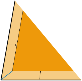
(a) Wide Kähler cone.

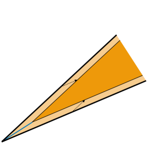
(b) Narrow Kähler cone.

Figure 1: Kähler and stretched Kähler cones $\mathcal{K}$ and $\widetilde{\mathcal{K}}$ for a two-dimensional setting. In figure 1(a) a wide cone is shown, while in figure 1(b) we have displayed a narrow Kähler cone. The darker shaded regions are the stretched Kähler cones with parameter $c$, and we have included the minimal distance $d_{\rm min}$ between the tip of the cone and the stretched cone for both cases.

Numerical results

Next, we recall some numerical results of [23] obtained for the Kreuzer-Skarke database [24]. The authors determined properties of the Kähler cone for Hodge numbers $h^{1,1}$ in the range $2\leq h^{1,1}\leq 491$ of the following form:

• The Kähler cone $\mathcal{K}_{\mathcal{Y}}$ is bounded by hypersurfaces which intersect the origin of moduli space. If the angle between these hypersurfaces is small, the Kähler cone is narrow. In figure 3 of [23] the dependence of the (cosine of the) smallest angle on $h^{1,1}$ is shown, and one sees that for large $h^{1,1}$ this angle tends to become small. Hence, for larger $h^{1,1}$ the Kähler cone becomes narrower.

• Another way to quantify the narrowness of the Kähler cone is to consider the stretched Kähler cone (4.12). This cone does not reach the origin of moduli space, and one can determine the point closest to it. The narrower the Kähler cone the further away the minimal point, as illustrated in figures 1. More concretely, in [23] the authors consider the stretched Kähler cone $\widetilde{\mathcal{K}}_{\cap}[c]$ and determine the minimal distance $d^{\cap}_{\rm min}[c]$ from the origin. This dependence on the Hodge numbers $h^{1,1}$ for $c=1$ is shown in figure 5 of [23] and has been fitted as

  $$\begin{split}d^{\cap}_{\rm min}[1]\simeq 10^{-1.4}\hskip 1.0pt(h^{1,1})^{2.5}\,.\end{split}$$ (4.14)

  Note that this data has been determined for $c=1$, however, $d^{\cap}_{\rm min}$ depends linearly on $c$. This implies we can generalize the above fit as

  $$\begin{split}d^{\cap}_{\rm min}[c]\simeq 10^{-1.4}\hskip 1.0pt(h^{1,1})^{2.5}\,c\,.\end{split}$$ (4.15)

• Finally, from figure 5 in [23] we can also determine an approximate lower bound in the region $h^{1,1}\gtrsim 10$ of the form

  $$\begin{split}d^{\cap}_{\rm min}[c]\gtrsim 10^{-2.6}\hskip 1.0pt(h^{1,1})^{2.7}\,c\,.\end{split}$$ (4.16)

Mirror symmetry

The complex-structure moduli space in the large complex-structure limit of a Calabi-Yau three-fold $\mathcal{X}$ is related to the Kähler moduli space of a Calabi-Yau manifold $\mathcal{Y}$ via mirror symmetry. For type IIB orientifolds discussed in this work the imaginary part of complex-structure moduli $z^{i}$ has to be inside a cone, which is the Kähler cone on a mirror three-fold. We refer to this cone as the complex-structure cone. From the results reviewed above, we can conclude that for large $h^{2,1}$ this cone becomes narrow. In particular, using the fit shown in (4.15) we can estimate the scaling of the minimal distance of the stretched cone to the origin as

$$\begin{split}d^{\rm cs}_{\rm min}[c]\simeq 10^{-1.4}\hskip 1.0pt(h^{2,1})^{2.5}\,c\,,\end{split}$$ (4.17)

where $c$ is the minimal distance away from the boundary of the ordinary cone. Similarly, the minimal distance away from the origin in a stretched Kähler cone is expected to satisfy the bound

$$\begin{split}d^{\rm cs}_{\rm min}\gtrsim 10^{-2.6}\hskip 1.0pt(h^{2,1})^{2.7}\,c\,.\end{split}$$ (4.18)

4.3 Implications for the tadpole conjecture

In section 3 we have argued that when approaching a boundary in moduli space, the flux number $N_{\rm flux}$ typically diverges. This applies in particular to a boundary of the complex-structure cone, and for obtaining a minimal $N_{\rm flux}$ one should therefore stabilize moduli in the interior of moduli space. However, in section 4.2 we have seen that for increasing $h^{2,1}$ the complex-structure cone becomes narrower and it becomes more difficult to avoid the boundary regions. Hence, for larger $h^{2,1}$ we expect an increase in $N_{\rm flux}$.

Setting

We now want to make this heuristic argument more concrete. Our main technical assumption for the following is that when the complex-structure cone becomes narrower, the increase of $N_{\rm flux}$ along a direction towards a boundary of the complex-structure cone is faster than along the large complex-structure direction. This implies that for larger $h^{2,1}$ one is pushed towards large complex-structure, when searching for a minimal flux number $N_{\rm flux}$. Or, in other words, we assume that the lowest value for $N_{\rm flux}$ is found inside a stretched complex-structure cone with parameter $c$ that is not too small.

Lower bound on $N_{\rm flux}$

Now, in equation (4.10) we have estimated that in the large complex-structure limit and for large $h^{2,1}$ the flux number for generic flux-compactifications behaves as

$$\begin{split}N_{\rm flux}\gtrsim(h^{2,1})^{1-\frac{\gamma}{2}}\hskip 1.0pt\lVert v\rVert^{\gamma}\,,\hskip 70.0pt\gamma=1,3\,,\end{split}$$ (4.19)

where $\lVert v\rVert$ denotes the Euclidean norm of $v^{i}=\mbox{Im}\,z^{i}$. We have furthermore argued that for large $h^{2,1}$ the complex-structure cone becomes narrow, and we determined in (4.18) a lower bound on the minimal distance of a stretched Kähler cone to the origin of moduli space. To obtain a minimal $N_{\rm flux}$ we therefore identify $\lVert v\rVert$ in (4.19) with $d^{\rm cs}_{\rm min}$ and obtain the lower bound

$$\begin{split}N_{\rm flux}[c]\gtrsim(h^{2,1})^{1-\frac{\gamma}{2}}\hskip 1.0pt\left[10^{-2.6}\hskip 1.0pt(h^{2,1})^{2.7}\,c\right]^{\gamma}\,,\hskip 50.0pt\gamma=1,3\,.\end{split}$$ (4.20)

This equation depends on the parameter $c$ which parametrizes the minimal distance from the stretched complex-structure cone to the boundary of the ordinary complex-structure cone (see figures 1). In particular, $c$ is the minimal volume of two-cycles on the mirror-dual side – and for having control over the world-sheet instanton corrections one expects that $c$ should not be much smaller than one. In view of our assumption stated above, we also expect that for small $c$ the effect of being close to a boundary leads to an increase in the flux number $N_{\rm flux}$.

Comparison with the tadpole conjecture

Within the approach we are following in this note we are not able to determine a precise value of $c$. We can however compare the behavior of $N_{\rm flux}[c]$ for different values of $c$ with the bound (1.1) of the tadpole conjecture. We have shown this comparison in figures 2, from which we see that for large $h^{2,1}$ the bound (4.20) exceeds the linear bound of the tadpole conjecture. For larger values of $c$ this crossover happens earlier, for smaller values of $c$ this happens later. In the large complex-structure and large $h^{2,1}$ regime, for moderate values of $c$ and for generic flux compactifications the tadpole conjecture is therefore satisfied.

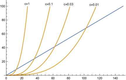
(a) Plot of $N_{\rm flux}$ for $\gamma=1$ and different values of $c$.

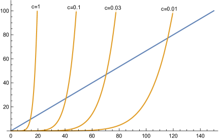
(b) Plot of $N_{\rm flux}$ for $\gamma=3$ and different values of $c$.

Figure 2: Comparison between the bound on $N_{\rm flux}$ shown in equation (4.20) (orange curves) and the bound from the tadpole conjecture (1.1) for $\alpha=1/3$ (blue curve). In figure 2(a) the parameter $\gamma$ is chosen as $\gamma=1$, while in figure 2(b) we have chosen $\gamma=3$.

Summary and remarks

We close this section with the following summary and remarks:

• We have estimated a bound on how the flux number $N_{\rm flux}$ depends on the dimension of the complex-structure moduli space in the large complex-structure and large $h^{2,1}$ regime. To do so, we first determined for generic situations the scaling of $N_{\rm flux}$ with $\lVert v\rVert$ which is shown in equation (4.10). Next, we have reviewed results of [23] on the geometry of the mirror-dual Kähler cone and how for large $h^{2,1}$ the corresponding complex-structure cone becomes narrow. Combining these observations we determined a lower bound on how $N_{\rm flux}$ depends on $h^{2,1}$, shown in equation (4.20).

• The bound in (4.20) depends on a parameter $c$, which parametrizes the minimal distance away from the boundary of the complex-structure cone. In order to trust the large complex-structure approximation, this parameter should not be taken much smaller than one. However, as shown in figures 2, even for values $c=0.1$ or $c=0.03$ we see that the flux number $N_{\rm flux}$ exceeds the linear behavior (1.1) of the tadpole conjecture for moderately-large values of $h^{2,1}$. We have then concluded that in the large complex-structure regime, the tadpole conjecture is satisfied for generic Calabi-Yau three-folds.

• We emphasize that the data in [23] is obtained for the Kreuzer-Skarke database, which is expected to represent generic features of Calabi-Yau three-folds. Furthermore, when estimating the scaling (4.10) we have used an average value of $\mathsf{v}^{i}\simeq(h^{2,1})^{-1/2}$ for the components of the normalized vector $\mathsf{v}^{i}$. We therefore have determined the generic behavior of $N_{\rm flux}$ in the large complex-structure and large $h^{2,1}$ regime, which may be different for specific non-generic constructions.

• Our main assumption in this section was that approaching a boundary of the complex-structure cone will lead to a faster increase of $N_{\rm flux}$ than approaching the large complex-structure point. In other words, when the complex-structure cone becomes narrower one is pushed towards the large complex-structure point. However, this assumption may not be true.

• Our analysis in this section has been carried out with the dilaton staying finite, in particular, $s$ does not scale with $h^{2,1}$. Such a scaling can be included, but for generic flux-configurations this will lead to an even stronger growth of $N_{\rm flux}$. However, for specific and fine-tuned flux choices the growth of $N_{\rm flux}$ may be reduced. An example is $h^{I}=0$, $f^{0}\neq 0$ and at least one $h_{i}\neq 0$, together with the assumptions that the Kähler metric $G_{i\overline{j}}$ is non-sparse and that the combinations $f^{i}-u^{i}\hskip 1.0ptf^{0}$ and $h_{0}+u^{i}h_{i}$ have a very specific dependence on $h^{2,1}$. It is a non-trivial question whether such configurations can be realized in concrete examples, and we consider such constructions to be non-generic.

5 Discussion

Let us now summarize and discuss our arguments of the previous sections, and make some further remarks and comments on the tadpole conjecture. We start with a brief summary:

• In section 3 we studied the boundary behavior of the flux number $N_{\rm flux}$. We argued that when approaching a boundary in complex-structure and axio-dilaton moduli space, this quantity typically diverges. We made this observation using a Bloch-Messiah decomposition of the Hodge-star matrix $\mathcal{M}$, however, the same result follows from asymptotic Hodge theory [21, 22, 6]. This implies, that a flux-configuration with minimal $N_{\rm flux}$ will stabilize moduli in the interior of moduli space, where one has typically less computational control. Hence, it can become challenging to explicitly test the tadpole conjecture made in [13].

• In section 4 we considered the large complex-structure limit and estimated a lower bond on the scaling of $N_{\rm flux}$ with $h^{2,1}$ for large $h^{2,1}$ and for generic situations. We obtained this bound using statistical data of [23] on how the complex-structure cone becomes narrower for larger $h^{2,1}$. For plausible choices of a parameter $c$, we find that our bound exceeds the bound of the tadpole conjecture for moderate values of $h^{2,1}$ (see figures 2), and therefore we find support for the conjecture in the large complex-structure regime. However, a configuration with a flux number $N_{\rm flux}$ that violates the tadpole conjecture may be outside of this regime.

We finally want to add further comments and remarks in view of the tadpole conjecture [13]:

• We emphasize that the bound obtained in (4.20) is not a proof of the tadpole conjecture. But, independent of this conjecture, it shows that for large $h^{2,1}$ and for generic flux-configurations, stabilizing all complex-structure and axio-dilaton moduli by fluxes in the large complex-structure regime in a consistent way is rather difficult.

• Even if isolated counter examples to the tadpole conjecture exist, the conjecture can have important implications for the size of the string-theory landscape. In particular, if the majority of string-compactifications does not allow for the stabilization of sufficiently many moduli, the landscape of effective four-dimensional theories with no or few massless scalar fields is smaller than naively expected.

• The constant $\alpha$ in the tadpole conjecture (1.1) has been proposed as $\alpha=1/3$, however, in [13] it is mentioned that the conjecture is often also satisfied for $\alpha\simeq 0.44$. We want to point out that deriving an exact numerical value for $\alpha$ appears to be difficult, since it emergences only at large $h^{2,1}$. Indeed, for $h^{2,1}=1$ one can find examples which stabilize the complex-structure modulus and the axio-dilaton with a flux number $N_{\rm flux}=1$, which would correspond to a value of $\alpha=1/4$. (We did this analysis for the conifold point of $X_{4,2}(1,1,1,1,1,1)$ which was discussed in [26].)

Acknowledgments

We thank Mariana Graña, Thomas Grimm, Damian van de Heisteeg and Viraf Mehta for very helpful discussions and communications. The work of EP is supported by a Heisenberg grant of the Deutsche Forschungsgemeinschaft (DFG, German Research Foundation) with project-number 430285316.

References

- [1] R. Bousso and J. Polchinski, “Quantization of four form fluxes and dynamical neutralization of the cosmological constant,” JHEP 06 (2000) 006, hep-th/0004134.
- [2] A. N. Schellekens, “Big Numbers in String Theory,” 1601.02462.
- [3] W. Lerche, D. Lüst, and A. N. Schellekens, “Chiral Four-Dimensional Heterotic Strings from Selfdual Lattices,” Nucl. Phys. B 287 (1987) 477.
- [4] W. Taylor and Y.-N. Wang, “The F-theory geometry with most flux vacua,” JHEP 12 (2015) 164, 1511.03209.
- [5] R. Blumenhagen, B. Körs, D. Lüst, and S. Stieberger, “Four-dimensional String Compactifications with D-Branes, Orientifolds and Fluxes,” Phys. Rept. 445 (2007) 1–193, hep-th/0610327.
- [6] T. W. Grimm, “Moduli Space Holography and the Finiteness of Flux Vacua,” 2010.15838.
- [7] B. Bakker, T. W. Grimm, C. Schnell, and J. Tsimerman, “to appear,”.
- [8] S. Kachru, R. Kallosh, A. D. Linde, and S. P. Trivedi, “De Sitter vacua in string theory,” Phys. Rev. D 68 (2003) 046005, hep-th/0301240.
- [9] V. Balasubramanian, P. Berglund, J. P. Conlon, and F. Quevedo, “Systematics of moduli stabilisation in Calabi-Yau flux compactifications,” JHEP 03 (2005) 007, hep-th/0502058.
- [10] I. Bena, E. Dudas, M. Graña, and S. Lüst, “Uplifting Runaways,” Fortsch. Phys. 67 (2019), no. 1-2 1800100, 1809.06861.
- [11] P. Betzler and E. Plauschinn, “Type IIB flux vacua and tadpole cancellation,” Fortsch. Phys. 67 (2019), no. 11 1900065, 1905.08823.
- [12] A. P. Braun and R. Valandro, “ flux, algebraic cycles and complex structure moduli stabilization,” JHEP 01 (2021) 207, 2009.11873.
- [13] I. Bena, J. Blåbäck, M. Graña, and S. Lüst, “The Tadpole Problem,” 2010.10519.
- [14] I. Bena, J. Blåbäck, M. Graña, and S. Lüst, “Algorithmically solving the Tadpole Problem,” 2103.03250.
- [15] F. Marchesano, D. Prieto, and M. Wiesner, “F-theory flux vacua at large complex structure,” 2105.09326.
- [16] M. Graña, “Flux compactifications in string theory: A Comprehensive review,” Phys. Rept. 423 (2006) 91–158, hep-th/0509003.
- [17] M. R. Douglas and S. Kachru, “Flux compactification,” Rev. Mod. Phys. 79 (2007) 733–796, hep-th/0610102.
- [18] S. Gukov, C. Vafa, and E. Witten, “CFT’s from Calabi-Yau four folds,” Nucl. Phys. B 584 (2000) 69–108, hep-th/9906070. [Erratum: Nucl.Phys.B 608, 477–478 (2001)].
- [19] E. Plauschinn, “The Generalized Green-Schwarz Mechanism for Type IIB Orientifolds with D3- and D7-Branes,” JHEP 05 (2009) 062, 0811.2804.
- [20] S. B. Giddings, S. Kachru, and J. Polchinski, “Hierarchies from fluxes in string compactifications,” Phys. Rev. D 66 (2002) 106006, hep-th/0105097.
- [21] W. Schmid, “Variation of Hodge structure: the singularities of the period mapping,” Invent. Math. 22 (1973) 211–319.
- [22] E. Cattani, A. Kaplan, and W. Schmid, “Degeneration of Hodge Structures,” Annals of Mathematics 123 (1986) 457.
- [23] M. Demirtas, C. Long, L. McAllister, and M. Stillman, “The Kreuzer-Skarke Axiverse,” JHEP 04 (2020) 138, 1808.01282.
- [24] M. Kreuzer and H. Skarke, “Complete classification of reflexive polyhedra in four-dimensions,” Adv. Theor. Math. Phys. 4 (2002) 1209–1230, hep-th/0002240.
- [25] M. Cicoli, D. Ciupke, C. Mayrhofer, and P. Shukla, “A Geometrical Upper Bound on the Inflaton Range,” JHEP 05 (2018) 001, 1801.05434.
- [26] A. Joshi and A. Klemm, “Swampland Distance Conjecture for One-Parameter Calabi-Yau Threefolds,” JHEP 08 (2019) 086, 1903.00596.