Anharmonic Lattice Dynamics from Vibrational Dynamical Mean-Field Theory

Abstract

We present a vibrational dynamical mean-field theory (VDMFT) of the dynamics of atoms in solids with anharmonic interactions. Like other flavors of DMFT, VDMFT maps the dynamics of a periodic anharmonic lattice of atoms onto those of a self-consistently defined impurity problem with local anharmonicity and coupling to a bath of harmonic oscillators. VDMFT is exact in the harmonic and molecular limits, nonperturbative, systematically improvable through its cluster extensions, usable with classical or quantum impurity solvers (depending on the importance of nuclear quantum effects), and can be combined with existing low-level diagrammatic theories of anharmonicity. When tested on models of anharmonic optical and acoustic phonons, we find that classical VDMFT gives good agreement with classical molecular dynamics, including the temperature dependence of phonon frequencies and lifetimes. Using a quantum impurity solver, signatures of nuclear quantum effects are observed at low temperatures. We test the description of nonlocal anharmonicity via cellular VDMFT and the combination with self-consistent phonon (SCPH) theory, yielding the powerful SCPH+VDMFT approach.

I Introduction

Since the seminal work of the early twentieth century, phonons have been foundational for the description of solids. However, early on it was recognized that anharmonic effects, corresponding to interactions between phonons, were nonnegligible and responsible for a variety of phenomena including thermal expansion, the stability of certain phases, the temperature dependence of phonon frequencies, phonon lifetimes, and thermal conductivity Clyde and Klein (1971); Klein and Horton (1972); Maris (1977); Fultz (2010); Grimvall et al. (2012). For example, many of the structural and dynamical properties of halide and oxide perovskites have been linked to their soft phonon modes and associated strong anharmonicity Yaffe et al. (2017); Marronnier et al. (2017); Zhou et al. (2018); Gold-Parker et al. (2018); Gehrmann and Egger (2019); Klarbring et al. (2020). Moreover, recent work has observed strongly correlated phonon behavior, such as Kondo-like phonon scattering in thermoelectric clathrates Ikeda et al. (2019) and the saturation or violation of Planckian bounds on thermal transport Wu and Sau (2021); Tulipman and Berg (2021).

Following on the self-consistent phonon (SCPH) theory Hooton (1958); Werthamer (1970); Klein and Horton (1972), a number of computational approaches have been developed to simulate the properties of anharmonic solids Souvatzis et al. (2008, 2009); Hellman et al. (2013); Errea et al. (2014); Tadano and Tsuneyuki (2015, 2018), most of which are static mean-field theories that seek an optimized harmonic description of anharmonic systems. Therefore, they yield improved thermodynamic properties and shifts in phonon frequencies, but cannot predict phonon lifetimes or non-quasiparticle effects. Such effects can be partially described using perturbation theory Maradudin and Fein (1962); Cowley (1965); Klemens (1966); Menéndez and Cardona (1984); Turney et al. (2009); Sun et al. (2010), which fails for strong anharmonicity, or by molecular dynamics (MD) Ladd et al. (1986); Tretiakov and Scandolo (2004); Turney et al. (2009); de Koker (2009); Sun et al. (2010), which is computationally expensive when accurate forces are used and requires approximate techniques to include nuclear quantum effects Ceriotti et al. (2009a); Dammak et al. (2009); Rossi et al. (2016); Cheng et al. (2018).

Here, we present a vibrational dynamical mean-field theory (VDMFT) without the above limitations—it is nonperturbative, exact in the harmonic and molecular limits, systematically improvable through cluster extensions, applicable to problems with or without nuclear quantum effects, and describes phonon spectra. Our VDMFT is completely analogous to conventional DMFT Georges and Kotliar (1992); Georges et al. (1996); Vollhardt (2011): it is a many-body theory of the phonon Green’s function (GF) Cowley (1963); Mahan (2000) that maps the dynamics of an anharmonic lattice onto those of a self-consistently defined impurity problem. In this way, VDMFT treats local anharmonicity nonperturbatively. Nonlocal anharmonicity can be included at lower-levels of theory and through cluster extensions of DMFT Hettler et al. (2000); Kotliar et al. (2001)—here we focus on cellular VDMFT.

The layout of this article is as follows. In Sec. II, we present the general theory of (cellular) VDMFT. In Sec. III, we present results for two problems. First, we study a model of optical phonons with local quartic anharmonicity, and we apply single-site VDMFT with both classical and quantum impurity solvers. Second, we study a model of acoustic phonons arising from pairwise Lennard-Jones interactions, and we demonstrate the convergence behavior of cellular VDMFT and the treatment of nonlocal anharmonicity at the mean-field level with SCPH theory. In Sec. IV, we conclude by identifying future directions.

II Theory

Within the Born-Oppenheimer approximation, the vibrational lattice Hamiltonian is

$$H=\sum_{{\bm{n}}\alpha}\frac{{\bm{p}}_{{\bm{n}}\alpha}^{2}}{2m_{\alpha}}+\mathcal{V}(\{{\bm{x}}_{{\bm{n}}\alpha}\})$$ (1)

where ${\bm{n}}$ are lattice translation vectors and $\alpha$ indexes atoms in the unit cell. We denote the thermal average with respect to this Hamiltonian as $\langle\cdots\rangle=\mathrm{Tr}[\cdots e^{-H/k_{\mathrm{B}}T}]/Z$ where $Z=\mathrm{Tr}e^{-H/k_{\mathrm{B}}T}$ is the canonical partition function. Expanding the anharmonic potential energy surface in terms of displacements away from the equilibrium lattice positions, ${\bm{u}}_{{\bm{n}}\alpha}={\bm{x}}_{{\bm{n}}\alpha}-\langle{\bm{x}}_{{\bm{n}}\alpha}\rangle$, naturally leads to the dynamical matrix

$$\mathcal{D}_{\alpha i,\beta j}({\bm{k}})=\frac{1}{\sqrt{m_{\alpha}m_{\beta}}}\sum_{({\bm{m}}-{\bm{n}})}e^{i{\bm{k}}\cdot({\bm{m}}-{\bm{n}})}\Phi_{{\bm{m}}\alpha i,{\bm{n}}\beta j}$$ (2)

where $\Phi_{{\bm{m}}\alpha i,{\bm{n}}\beta j}=\partial^{2}\mathcal{V}/\partial u_{{\bm{m}}\alpha i}\partial u_{{\bm{n}}\beta j}$ is the force constant matrix evaluated at the equilibrium lattice positions and $i,j$ are Cartesian coordinates. In this noninteracting limit or in static mean-field theories of anharmonicity, an eigenvalue problem

$$\left[\bm{\mathcal{D}}({\bm{k}})+\bm{\mathcal{W}}({\bm{k}})\right]\mathbf{c}_{\lambda}({\bm{k}})=\Omega^{2}_{\lambda}({\bm{k}})\mathbf{c}_{\lambda}({\bm{k}}),$$ (3)

defines a set of phonon frequencies $\Omega_{\lambda}({\bm{k}})$ and collective coordinates

$$u_{\lambda}({\bm{k}})=N^{-1/2}\sum_{{\bm{n}}\alpha i}\sqrt{m_{\alpha}}c_{{\bm{n}}\alpha i,\lambda}({\bm{k}})e^{-i{\bm{k}}\cdot{\bm{n}}}u_{{\bm{n}}\alpha i}$$ (4)

for phonon branch $\lambda$, where $\bm{\mathcal{W}}({\bm{k}})$ is the optional mean-field contribution (see Sec. III.2 for an example use of SCPH mean-field theory). For notational convenience, we define an effective harmonic matrix in the Cartesian basis $\mathbf{\Omega}^{2}({\bm{k}})\equiv\bm{\mathcal{D}}({\bm{k}})+\bm{\mathcal{W}}({\bm{k}})$.

Our object of interest in VDMFT is the finite-temperature phonon GF

$$i\hbar D_{\lambda\lambda^{\prime}}({\bm{k}},\omega+i\eta)=\int_{0}^{\infty}dte^{i(\omega+i\eta)t}\langle[u_{\lambda}({\bm{k}},t),u_{\lambda^{\prime}}(-{\bm{k}},0)]\rangle;$$ (5)

henceforth we drop $i\eta$ for notational simplicity and warn that the GF $\mathbf{D}({\bm{k}},\omega)$ should not be confused with the dynamical matrix $\bm{\mathcal{D}}({\bm{k}})$. Defining the corresponding harmonic GF via $\mathbf{D}_{0}^{-1}({\bm{k}},\omega)=\omega^{2}\mathbf{1}-\mathbf{\Omega}^{2}({\bm{k}})$, the interacting phonon GF is given by

$$\mathbf{D}^{-1}({\bm{k}},\omega)=\mathbf{D}_{0}^{-1}({\bm{k}},\omega)-2\mathbf{\Omega}({\bm{k}})\bm{\pi}({\bm{k}},\omega)$$ (6)

where $\bm{\pi}({\bm{k}},\omega)$ is the phonon self-energy.

Standard perturbative approaches evaluate the self-energy $\bm{\pi}({\bm{k}},\omega)$ up to second order in the anharmonicity using cubic and/or quartic anharmonic force constants of the potential $\mathcal{V}$ Tadano and Tsuneyuki (2015, 2018). Instead, in VMDFT we neglect the momentum dependence of the self-energy term $\mathbf{\Omega}({\bm{k}})\bm{\pi}({\bm{k}},\omega)\approx\mathbf{\Omega}\bm{\pi}(\omega)$, which is obtained nonperturbatively from a self-consistently defined impurity problem (the impurity frequency matrix $\mathbf{\Omega}$ will be defined below). The Hamiltonian of the impurity problem is of the Caldeira-Leggett form Caldeira and Leggett (1983), $H_{\mathrm{imp}}=H_{\mathrm{s}}+H_{\mathrm{b}}+H_{\mathrm{sb}}$ with

$$H_{\mathrm{s}} =\sum_{\alpha}\frac{{\bm{p}}_{\alpha}^{2}}{2m_{\alpha}}+V_{\mathrm{loc}}(\{{\bm{u}}_{\alpha}\})$$ (7a)

$$H_{\mathrm{b}} =\frac{1}{2}\sum_{m}\left(p_{m}^{2}+\omega_{m}^{2}x_{m}^{2}\right)$$ (7b)

$$H_{\mathrm{sb}} =\sum_{\alpha im}c_{\alpha i,m}u_{\alpha i}x_{m},$$ (7c)

where $(p_{m},x_{m})$ are degrees of freedom of a bath of harmonic oscillators and the local potential $V_{\mathrm{loc}}$ includes bare harmonic and anharmonic interactions within the cell and the local, harmonic parts of the nonlocal interactions across the cell boundary (possibly at the mean-field level). The harmonic bath is completely specified by the hybridization function $\bm{\Delta}(\omega)$, which captures the influence of the lattice on the dynamics of the cluster and is defined by

$$2\mathbf{\Omega}\bm{\Delta}(\omega)=\omega^{2}\mathbf{1}-\mathbf{\Omega}^{2}-2\mathbf{\Omega}\bm{\pi}(\omega)-\mathbf{D}_{\mathcal{C}}^{-1}(\omega),$$ (8)

where $\mathbf{D}_{\mathcal{C}}(\omega)=N^{-1}\sum_{\bm{k}}\mathbf{D}({\bm{k}},\omega)$ is the cellular GF and $N$ is the number of cells in the Born-von Karman supercell. The effective dynamical matrix of the impurity $\mathbf{\Omega}^{2}$ is determined by the harmonic part of $V_{\mathrm{loc}}$. The impurity Hamiltonian (7) is related to the hybridization by the spectral density $\mathbf{J}(\omega)=-2\mathrm{Im}\mathbf{\Omega}\bm{\Delta}(\omega)$ or

$$J_{\alpha i,\beta j}(\omega)=\frac{\pi}{2}\sum_{m}\frac{c_{\alpha i,m}c_{\beta j,m}}{\omega_{m}}\left[\delta(\omega-\omega_{m})-\delta(\omega+\omega_{m})\right].$$ (9)

By construction, the hybridization is exact when the lattice and impurity problems are treated at the same level of theory (for example, in the harmonic limit, the bath construction is a simple normal mode transformation of the lattice degrees of freedom). The power of DMFT lies in the fact that an accurate treatment of the dynamics of the impurity problem (7) is far more tractable than that of the anharmonic lattice problem. In this case, where the lattice and impurity problems are treated at different levels of theory, a self-consistent solution must be obtained.

Various impurity solvers, discussed more below, can be used to calculate the anharmonic impurity GF and phonon self-energy,

$$i\hbar[\mathbf{D}_{\mathrm{imp}}(t)]_{\alpha i,\beta j} =\theta(t)\langle[u_{\alpha i}(t),u_{\beta j}(0)]\rangle,$$ (10)

$$2\mathbf{\Omega}\bm{\pi}(\omega) =\mathbf{d}_{\mathrm{imp}}^{-1}(\omega)-\mathbf{D}_{\mathrm{imp}}^{-1}(\omega),$$ (11)

where $\mathbf{d}_{\mathrm{imp}}^{-1}(\omega)=\omega^{2}\mathbf{1}-\bm{\Omega}^{2}-2\bm{\Omega}\bm{\Delta}(\omega)$ is the harmonic impurity GF. Within the DMFT approximation, this phonon self-energy defines the lattice GF $\mathbf{D}({\bm{k}},\omega)$ and thus the cellular GF, the hybridization via Eq. (8), and the impurity problem itself. This establishes the VDMFT self-consistency condition $\mathbf{D}_{\mathcal{C}}(\omega)=\mathbf{D}_{\mathrm{imp}}(\omega)$. In practice, we make an initial guess of the self-energy and iterate the VDMFT loop until convergence. Note that with a straightforward redefinition of the size of a unit cell, the above equations also describe the cellular VDMFT approach for including short-range nonlocal anharmonicity exactly. Because cellular DMFT breaks translational symmetry (beyond a single-cell cluster), we periodize the converged self-energy to study lattice quantities Kotliar et al. (2001); Parcollet et al. (2004); Civelli et al. (2005), as discussed below.

Because phonons formally obey Bose-Einstein statistics, our VDMFT has many similarities to bosonic DMFT Hu and Tong (2009); Anders et al. (2011). However, the number of phonons in solids is not conserved, unlike interacting lattice bosons such as cold atoms. Thus, equilibrium condensation is not a primary concern, unlike in most applications of bosonic DMFT. Note that if the equilibrium atomic positions are approximated by their zero-temperature values that minimize the potential energy $\langle{\bm{x}}_{{\bm{n}}\alpha}\rangle\approx{\bm{x}}_{{\bm{n}}\alpha}^{(0)}$, then a structural phase transition occurring at elevated temperature is consistent with $\langle{\bm{u}}_{{\bm{n}}\alpha}\rangle\neq 0$, which is sometimes described as condensation. In such cases, an explicit treatment of condensation within VDMFT might be worthwhile. However, this concern is removed as long as the equilibrium positions are properly redefined Yukalov (2012). We note that the equilibrium atomic positions are a static property, which is far easier to calculate than a dynamical one, such as the Green’s function. In principle, the equilibrium atomic positions can be self-consistently defined as those that minimize the VDMFT vibrational free energy or that of simpler theories such as SCPH. Moreover, most vibrational problems in solids can be treated without regard for particle statistics (classically or quantum mechanically), and these are the target problems for VDMFT.

III Results

III.1 Optical phonons: Single-site VDMFT

To illustrate VDMFT, we first consider a one-dimensional chain of oscillators with mass $m=1$, periodic boundary conditions, and purely local anharmonicity,

$$H=\sum_{n=1}^{N}\left[\frac{p_{n}^{2}}{2}+\frac{1}{2}\Omega_{0}^{2}u_{n}^{2}+gu_{n}^{4}\right]+\frac{1}{2}\omega_{0}^{2}\sum_{n=1}^{N}(u_{n}-u_{n+1})^{2}.$$ (12)

For the quartic anharmonicity considered here, all frequency shifts and lifetimes are due to four-phonon processes or higher. Physically, this Hamiltonian could model a molecular crystal with anharmonic intramolecular vibrations and harmonic intermolecular vibrations. Here and throughout we assume a fixed volume, such that there is no thermal expansion. We emphasize that, given the mean-field nature of VDMFT, the one-dimensional models studied here provide a challenging test. The optical phonons of the Hamiltonian (12) are $u(k)=N^{-1/2}\sum_{n}e^{-ikn}u_{n}$ with the noninteracting harmonic dispersion $\Omega^{2}(k)=\Omega_{0}^{2}+4\omega_{0}^{2}\sin^{2}(k/2)$. Within single-site VDMFT, the impurity Hamiltonian has components

$$H_{\mathrm{s}} =\frac{p^{2}}{2}+\frac{1}{2}\Omega_{0}^{2}u^{2}+gu^{4}+\omega_{0}^{2}u^{2}\equiv\frac{p^{2}}{2}+V_{\mathrm{loc}}(u)$$ (13a)

$$H_{\mathrm{b}} =\tfrac{1}{2}\sum_{m}\left(p_{m}^{2}+\omega_{m}^{2}x_{m}^{2}\right)$$ (13b)

$$H_{\mathrm{sb}} =u\sum_{m}c_{m}x_{m},$$ (13c)

where $J(\omega>0)=(\pi/2)\sum_{m}c_{m}^{2}/\omega_{m}\delta(\omega-\omega_{m})$. Note that the local potential includes a harmonic term $\omega_{0}^{2}u^{2}$ arising from the nonlocal interaction across the cell boundary such that $\Omega=[\Omega_{0}^{2}+2\omega_{0}^{2}]^{1/2}$ is the harmonic impurity frequency.

We first assess the performance of VDMFT with a classical impurity solver. In this classical limit, the dynamics of the harmonic bath can be integrated out such that the impurity position satisfies the generalized Langevin equation (GLE),

$$\ddot{u}(t)=-\frac{dV_{\mathrm{eff}}}{du}-\int_{0}^{t}ds\gamma(t-s)\dot{u}(s)+\xi(t)$$ (14)

where $\gamma(t)=(2/\pi)\int_{0}^{\infty}d\omega\cos(\omega t)J(\omega)/\omega$ is a memory kernel, $V_{\mathrm{eff}}(u)=V_{\mathrm{loc}}(u)-\gamma(t=0)u^{2}/2$ is the local potential with a bath-induced renormalization Weiss (2012), and $\xi(t)$ is a random force satisfying detailed balance $\langle\xi(t)\xi(s)\rangle=k_{\mathrm{B}}T\gamma(t-s)$. In this formulation, the lattice hybridization can be seen to play the role of a very specific colored-noise thermostat Ceriotti et al. (2009a, 2010). As described in App. A, we solve the GLE numerically Tuckerman and Berne (1993); Ceriotti et al. (2010) to yield an ensemble of trajectories from which we calculate the classical one-sided impurity autocorrelation function $C_{\mathrm{cl}}(t)=\langle u(t)u(0)\rangle$. The impurity GF is then calculated as

$$D_{\mathrm{imp}}(t)=-\frac{1}{\hbar\pi}\theta(t)\int_{-\infty}^{\infty}d\omega\sin(\omega t)C_{\mathrm{cl}}(\omega)Q(\omega,T)$$ (15)

where $Q(\omega,T)=(\hbar\omega/k_{\mathrm{B}}T)(1-e^{-\hbar\omega/k_{\mathrm{B}}T})^{-1}$ is a temperature-dependent quantum correction factor that makes $D_{\mathrm{imp}}(t)$ exact in the harmonic limit Bader and Berne (1994).

For the Hamiltonian (12), we take the harmonic frequency of the intercellular potential $\omega_{0}$ as the unit of energy and set $\hbar=k_{\mathrm{B}}=1$. We use a local harmonic frequency $\Omega_{0}/\omega_{0}=1.3$ and anharmonicity $g/\omega_{0}^{3}=4.3$. In Figs. 1(a) and (b), we show the converged momentum-resolved spectral function $A(k,\omega)=-\pi^{-1}\mathrm{Im}D(k,\omega)$ at $T/\omega_{0}=1.3$ obtained from VDMFT (a) and from exact MD simulations of the full lattice problem (b) ; the agreement is excellent. (At this low temperature, nuclear quantum effects are significant—see below—but we can still assess the accuracy of VDMFT within the consistent approximation of classical dynamics.) For these parameters, the VDMFT loop converged in about four iterations when initialized by neglecting the self-energy. As expected, the peaks of the spectral functions are significantly shifted from the harmonic dispersion and are broadened due to phonon lifetime effects. In Fig. 1(c), we show the total vibrational density of states (DOS), $N^{-1}\sum_{k}A(k,\omega)$, at increasing temperatures ranging from $T/\omega_{0}=1.3$ to $T/\omega_{0}=15.5$. As is well known, the harmonic DOS is independent of temperature. The agreement between VDMFT and MD is seen to be excellent at all temperatures and the DOS shows decreasing lifetimes and phonon hardening with increasing temperature, as expected for a potential with quartic anharmonicity. The remarkable accuracy of single-site VDMFT for this problem can be largely attributed to the purely local form of the anharmonicity. Importantly, the computational cost of solving the GLE (14) for a single degree of freedom is significantly less than that of MD for the system sizes needed to obtain converged results.

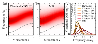
Figure 1: Single-site VDMFT results for the Hamiltonian (12) with a classical impurity solver. (a),(b) Spectral functions from VDMFT and MD, respectively, at $T/\omega_{0}=1.3$, compared to the harmonic dispersion (dashed grey line). (c) Temperature-dependent density of states (DOS) obtained from harmonic theory (dashed grey), VDMFT (yellow to red), and “exact” molecular dynamics (MD, thin solid black). In all results, $\eta/\omega_{0}=0.02$.

Next, we consider the possible importance of nuclear quantum effects, which can be straightforwardly included in VDMFT with a quantum impurity solver. Here, we use the hierarchical equations of motion Tanimura and Kubo (1989); Ishizaki and Tanimura (2005), which is a numerically exact technique for simulating the dynamics of systems coupled to harmonic baths; more details are given in App. B. In Fig. 2(a), we show the spectral function for the same parameters as in Figs. 1(a),(b); unlike in the classical case, the quantum case is a large many-body problem without a numerically tractable exact solution. We see that the quantum spectral function is narrower and more structured than the classical one, indicating that nuclear quantum effects are indeed important at this relatively low temperature $T/\omega_{0}=1.3$. Accurate quantum vibrational spectra of a condensed-phase system are extremely hard to obtain by other means.

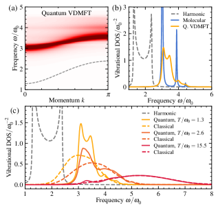
Figure 2: Single-site VDMFT results for the Hamiltonian (12) with a quantum impurity solver. (a) Quantum spectral function for the same temperature as in Figs. 1(a),(b). (b) At the same temperature, the DOS from harmonic theory (dashed grey), the molecular limit of a single anharmonic oscillator (blue), and quantum VDMFT (yellow). (c) DOS at increasing temperature (yellow to red) obtained by VDMFT with a quantum (solid) and classical (dashed) impurity solver. In all results, $\eta/\omega_{0}=0.02$.

To understand the origin of the structured spectral features, in Fig. 2(b), we compare the lattice DOS to the analogous quantum spectrum for a single anharmonic site (the so-called atomic or molecular limit) with potential $V(u)=\frac{1}{2}\Omega_{0}^{2}u^{2}+gu^{4}$,

$$-\pi^{-1}\mathrm{Im}\ d(\omega)=\sum_{ab}(P_{a}-P_{b})|\langle\psi_{a}|u|\psi_{b}\rangle|^{2}\delta\big{(}\omega-(E_{b}-E_{a})\big{)},$$ (16)

where $|\psi_{a}\rangle$, $E_{a}$ are eigenstates and eigenvalues of the anharmonic oscillator and $P_{a}=e^{-E_{a}/T}/\sum_{b}e^{-E_{b}/T}$. The peaks in the molecular spectrum are thus due to transitions between eigenstates of the anharmonic oscillator with intensities depending on their Boltzmann weights and transition matrix elements. These discrete quantum transitions are responsible for the structure seen in the lattice DOS when a quantum impurity solver is used. In Fig. 2(c), we compare the quantum and classical DOS at three temperatures spanning the same range as in Fig. 1(c). At low temperatures, we see the discrepancy due to the importance of nuclear quantum effects. However, at high temperatures, we see that the quantum and classical spectral functions agree due to the diminishing importance of nuclear quantum effects.

III.2 Acoustic phonons: Cellular VDMFT

Consider now the vibrational Hamiltonian with nonlocal anharmonicity due to a pair potential,

$$H=\sum_{n=1}^{N}\left[\frac{p_{n}^{2}}{2}+V(u_{n}-u_{n+1})\right]$$ (17)

Due to its invariance to infinitesimal translations, the above Hamiltonian will exhibit a single acoustic phonon branch; the noninteracting harmonic dispersion is $\Omega(k)=2\omega_{0}\lvert\sin(k/2)\rvert$ where $\omega_{0}$ is the harmonic frequency of the pair potential $V$.

Treating the nonlocal interactions encoded in a pair potential requires a cluster VDMFT, such as the cellular extension described above. In the impurity Hamiltonian of cellular VDMFT, we keep only the local, harmonic parts of the nonlocal interactions that cross the boundary of the cluster. In principle, we could also keep local, anharmonic parts of these interactions. However, doing so breaks the symmetry associated with infinitesimal translations and incorrectly opens a gap at the $\Gamma$ point (note that periodization only restores lattice translational symmetry). Here, we study the convergence of cellular VDMFT with cluster size $N_{\mathrm{c}}$, using classical impurity solvers, ranging from $N_{\mathrm{c}}=2\text{--}4$. After convergence of the DMFT cycle, we calculate the momentum-resolved spectral function using a periodized self-energy term Kotliar et al. (2001); Parcollet et al. (2004); Civelli et al. (2005),

$$\Omega(k)\pi(k,\omega)=N_{\mathrm{c}}^{-1}\sum_{\alpha\beta}[\bm{\Omega\pi}(\omega)]_{\alpha\beta}e^{ik(\alpha-\beta)},$$ (18)

although other choices are possible Stanescu and Kotliar (2006); Sakai et al. (2012).

Figure 3: Cellular VDMFT results for the Hamiltonian (17) with a Lennard-Jones potential truncated at fourth order at $T/\omega_{0}=2.7$. (a) Spectral function at $k=\pi$ obtained from the bare harmonic theory (dashed light blue), SCPH theory (dashed light green), and their combinations with cellular VDMFT as a function of cluster size ($N_{\mathrm{c}}=2,3,4$, light to dark), compared to the exact MD result (solid black). (b) Spectral function from SCPH+VDMFT with $N_{\mathrm{c}}=4$ and (c) from MD. In all results, $\eta/\omega_{0}=0.01$.

Results of cellular VDMFT are shown in Fig. 3 using a Lennard-Jones pair potential with its minimum at the lattice spacing and its harmonic frequency $\omega_{0}$ taken as the unit of energy. For simplicity, the potential is truncated to include only cubic and quartic anharmonicity. Results are shown at temperature $T/\omega_{0}=2.7$, where we do not expect significant nuclear quantum effects. In Fig. 3(a), we show the spectral function at the zone boundary $k=\pi$. We see that as the cluster size increases, cellular VDMFT yields a spectral function that approaches the exact one from MD. However, the convergence is slow because of the poor accuracy of the bare harmonic GF $D_{0}(k,\omega)$, which completely neglects nonlocal anharmonicity.

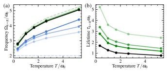
Figure 4: (a) Temperature-dependent phonon frequency $\Omega_{k}$ and (b) phonon lifetime $\tau_{k}$ at the Brillouin zone boundary $k=\pi$ for the same Lennard-Jones system as in Fig. 3. Colors and linetypes are the same as in Fig. 3.

For better performance, we can treat nonlocal anharmonicity with an improved low-level GF such as the one from SCPH theory (i.e., mean-field theory in the anharmonicity). For this simple model, the SCPH self-energy is diagonal. Considering only cubic and quartic anharmonicity, only the latter contributes to first order in a loop diagram and the SCPH phonon frequencies $\Omega(k)$ are determined self-consistently according to

$$\Omega^{2}(k) =\omega^{2}(k)+\mathcal{W}(k)\equiv\omega^{2}(k)+2\Omega(k)\pi^{(0)}(k)$$ (19a)

$$\pi^{(0)}(k) =k_{\mathrm{B}}T\sum_{k^{\prime}}\frac{\Phi(k,-k,k^{\prime},-k^{\prime})}{4\Omega(k)\Omega^{2}(k^{\prime})},$$ (19b)

where $\mathcal{W}(k)$ is the static mean-field contribution introduced in Eq. (3) and

$$\Phi(k,-k,k^{\prime},-k^{\prime})=N^{-1}\sum_{n_{2},n_{3},n_{4}}\frac{\partial^{4}\mathcal{V}}{\partial u_{0}\partial u_{n_{2}}\partial u_{n_{3}}\partial u_{n_{4}}}e^{-ikn_{2}+ik^{\prime}(n_{3}-n_{4})}$$ (20)

is the quartic force constant. In the above, we have taken the high-temperature limit of classical statistics and relabeled the noninteracting phonon frequencies as $\omega(k)$ to distinguish them from the SCPH frequencies $\Omega(k)$. Using the SCPH GF in place of the noninteracting GF in the VDMFT equations defines the SCPH+VDMFT method. In this way, the SCPH+VDMFT method treats local anharmonicity exactly and nonlocal quartic anharmonicity at the mean-field level, analogous to the use of Hartree-Fock+DMFT for fermionic problems. Note that the diagrammatic formulation of SCPH theory ensures a rigorous combination with VDMFT without the need for double-counting corrections Haule (2015); Karolak et al. (2010).

The SCPH+VDMFT spectral function at the zone boundary is shown in Fig. 3(a) with increasing cluster size. Because of the improved performance of SCPH theory, the convergence with cluster size is significantly improved. In Fig. 4, we study this performance as a function of temperature, plotting the phonon frequency (a) and lifetime (b) obtained by the harmonic theory (with no temperature dependence), SCPH theory (with infinite lifetime, characteristic of static mean-field theories), and the two flavors of VDMFT, compared to exact results from MD; all lifetimes were determined by a fit to a Lorentzian lineshape function. The exact MD lifetimes $\tau_{k=\pi}\omega_{0}\approx 1$ are indicative of nearly incoherent phonon dynamics that are beyond the limits of perturbation theory. Clearly, SCPH+VDMFT is a significant improvement for the phonon frequency, and the cellular results converge quickly to the exact MD result. The SCPH+VDMFT lifetime is not yet converged, and the value for our largest cluster size exhibits an error of about 50%. We do not consider the harmonic+VDMFT lifetime because the lineshape is significantly asymmetric, as can be seen in Fig. 3(a).

IV Conclusions and future work

We have introduced vibrational DMFT, including a cellular extension and the combination with approximate low-level theories, which demonstrates that VDMFT is not a replacement for existing theories of anharmonicity, but rather a formalism that enables their systematic and nonperturbative improvement. Future work will test alternative impurity solvers and cluster methods Hettler et al. (2000), as well as the performance in higher dimensions and for other observables such as the free energy Sham (1965); Plakida and Siklós (1978) and thermal conductivities Pang et al. (2013); Liao et al. (2015); Zhou et al. (2018); Gold-Parker et al. (2018). Moreover, VDMFT could be adapted for use in problems with coupling between electronic and bosonic degrees of freedom, such as those with physical electron-phonon coupling de Koker (2009) or those arising in extended DMFT to treat nonlocal interactions Pankov et al. (2002); Akerlund et al. (2014).

VDMFT can be extended to atomistic materials, either with model Hamiltonians Ai et al. (2014); Chen et al. (2014) or in a fully ab initio framework. In the latter case, force-fields or electronic structure theory can be used to determine the anharmonic potential energy surface; in particular, the small size of a unit cell will enable the use of highly accurate electronic structure methods that would otherwise be too costly for explicit MD of large supercells. The anharmonic impurity problem can then be solved using thermostatted MD Ceriotti et al. (2009a, 2010) or efficient quantum configuration interaction approaches Neff and Rauhut (2009); Fetherolf and Berkelbach (2021). Work along all of these lines is currently in progress.

Appendix A Classical vibrational impurity solver

For the nearest-neighbor interactions considered in the manuscript, only the boundary atoms of cellular VDMFT are coupled to the bath. Therefore, the interior atoms $\alpha$ and boundary atoms $\beta$ obey the coupled equations of motion

$$\ddot{u}_{\alpha}(t) =-\frac{dV_{\mathrm{eff}}}{du_{\alpha}}$$ (21a)

$$\ddot{u}_{\beta}(t) =-\frac{dV_{\mathrm{eff}}}{du_{\beta}}-\int_{0}^{t}ds\gamma_{\beta}\left(t-s\right)\dot{u}_{\beta}\left(s\right)+\xi_{\beta}(t),$$ (21b)

where the random force satisfies detailed balance $\langle\xi_{\beta}(t)\xi_{\beta}(s)\rangle=k_{\mathrm{B}}T\gamma_{\beta}(t-s)$. As described, e.g., in Ref. Tuckerman and Berne, 1993, $\xi_{\beta}(t)$ can be expressed by a Fourier decomposition, the components of which are sampled from a Gaussian distribution with a variance equal to the Fourier transform of the memory kernel. For each random sampling, a trajectory of length $T$ timesteps can be calculated via explicit integration of the coupled integrodifferential equations (21). However, this introduces an $O(T)$ storage cost and $O(T^{2})$ computational cost. To eliminate these costs, we simulate the non-Markovian dynamics via Markovian dynamics in an extended phase-space Marchesoni and Grigolini (1983); Ceriotti et al. (2009b, 2010).

For each physical boundary coordinate, $u_{\beta}$, we add a set of $n$ auxiliary momenta ${s}_{i}^{\beta}$, which have bilinear coupling to the physical momentum and among themselves. Decomposing the memory kernel in the form

$$\gamma_{\beta}(t)=\sum_{i=1}^{n}\sum_{j=1}^{n}a_{i}^{\beta}[e^{-\mathbf{A}^{\beta}t}]_{ij}a_{j}^{\beta}=[\bm{a}^{\beta}]^{\mathrm{T}}e^{-\mathbf{A}^{\beta}t}\bm{a}^{\beta},$$ (22)

where $\mathbf{A}^{\beta}$ is a real, anti-symmetric matrix whose complex eigenvalues have a positive real part, the equations of motion for the $(1+n)$ momenta are

$$\ddot{u}_{\beta}(t) =-\frac{dV_{\mathrm{eff}}}{du_{\beta}}-\sum_{j=1}^{n}{a}_{j}^{\beta}s_{j}^{\beta}(t),$$ (23a)

$$\dot{s}_{i}^{\beta}(t) ={a}_{i}^{\beta}\dot{u}_{\beta}(t)-\sum_{j=1}^{n}{A}_{ij}^{\beta}s_{j}^{\beta}(t)+\sqrt{2k_{\mathrm{B}}TA_{ii}^{\beta}}\ {\zeta}_{i}^{\beta}(t),$$ (23b)

where $\langle\zeta_{i}^{\beta}(t)\zeta_{j}^{\beta}(s)\rangle=\delta_{ij}\delta(t-s)$.

A numerically convenient decomposition of the Fourier transform of the memory kernel,

$$\gamma(\omega)=\frac{2}{\pi}\sum_{i=1}^{m}\frac{\eta_{i}\gamma_{i}(\omega^{2}+\omega_{i}^{2}+\gamma_{i}^{2})}{[(\omega+\omega_{i})^{2}+\gamma_{i}^{2}][(\omega-\omega_{i})^{2}+\gamma_{i}^{2}]},$$ (24)

can be achieved with a simple structure of $\bm{a}^{\beta}$ and $\mathbf{A}^{\beta}$ in terms of pairs of modes,

$$a^{\beta}_{2i-1}=a^{\beta}_{2i} =\sqrt{\eta_{i}/2\pi}$$ (25a)

$$A^{\beta}_{2i-1,2i-1}=A^{\beta}_{2i,2i} =\gamma_{i}$$ (25b)

$$A^{\beta}_{2i-1,2i}=-A^{\beta}_{2i,2i-1} =\omega_{i}$$ (25c)

such that there are $n=2m$ auxiliary momenta. In the results presented in the manuscript, we use the above form to numerically fit the memory kernel with up to $m=14$ modes (i.e., $n=28$ auxiliary momenta).

Appendix B Quantum vibrational impurity solver

First, we use grid techniques to numerically solve the Schrödinger equation for the anharmonic subsystem Hamiltonian $H_{\mathrm{s}}$ and keep the lowest $N_{\mathrm{s}}$ eigenstates $\psi_{a}(u)=\langle u|\psi_{a}\rangle$, depending on temperature. For the results presented in the manuscript, we kept up to $N_{\mathrm{s}}=18$ eigenstates. The eigenstates are then transformed to a discrete variable representation Light et al. (1985), $|d\rangle=\sum_{a}U_{ad}|\psi_{a}\rangle$ that diagonalizes the position operator and thus makes the system-bath Hamiltonian diagonal,

$$H_{\mathrm{s}} =\sum_{dd^{\prime}}|d\rangle H_{dd^{\prime}}\langle d^{\prime}|$$ (26a)

$$H_{\mathrm{sb}} =\sum_{d}|d\rangle u_{d}\langle d|\sum_{m}c_{m}x_{m}$$ (26b)

where $u_{d}=\int du\ u\ |\phi_{d}(u)|^{2}$. The quantum correlation function is then calculated as $\langle U(t)U(0)\rangle$ where $U=\sum_{d}|d\rangle u_{d}\langle d|$.

To simulate the quantum dynamics of an $N_{\mathrm{s}}$-level system linearly coupled to a bath of harmonic oscillators, we use the hierarchical equations of motion method Tanimura and Kubo (1989); Ishizaki and Tanimura (2005) as implemented in the pyrho package developed in our group pyr (2020). Similar to the classical impurity solver, the spectral density of the bath is numerically fit to a sum of underdamped Lorentzian modes Liu et al. (2014),

$$J(\omega)=\sum_{i=1}^{m}\frac{\eta_{i}\omega}{[(\omega+\omega_{i})^{2}+\gamma_{i}^{2}][(\omega-\omega_{i})^{2}+\gamma_{i}^{2}]};$$ (27)

for the results in the manuscript, we used up to $m=8$ modes. To simulate the thermal correlation function, we first propagated the system and auxiliary density matrices starting from a factorized initial condition, until reaching equilibrium; this set of density matrices was then used as the initial condition for the dynamics of the correlation function. All results were found to be converged with the hierarchy truncated at level $L=4$ and $K=0$ Matsubara frequencies.

References

- Clyde and Klein (1971) H. R. Clyde and M. L. Klein, Crit. Rev. Solid State Mater. Sci. 2, 181 (1971).
- Klein and Horton (1972) M. L. Klein and G. K. Horton, J. Low Temp. Phys. 9, 151 (1972).
- Maris (1977) H. J. Maris, Rev. Mod. Phys. 49, 341 (1977).
- Fultz (2010) B. Fultz, Prog. Mater Sci. 55, 247 (2010).
- Grimvall et al. (2012) G. Grimvall, B. Magyari-Köpe, V. Ozoliņš, and K. A. Persson, Rev. Mod. Phys. 84, 945 (2012).
- Yaffe et al. (2017) O. Yaffe, Y. Guo, L. Z. Tan, D. A. Egger, T. Hull, C. C. Stoumpos, F. Zheng, T. F. Heinz, L. Kronik, M. G. Kanatzidis, J. S. Owen, A. M. Rappe, M. A. Pimenta, and L. E. Brus, Phys. Rev. Lett. 118, 136001 (2017).
- Marronnier et al. (2017) A. Marronnier, H. Lee, B. Geffroy, J. Even, Y. Bonnassieux, and G. Roma, J. Phys. Chem. Lett. 8, 2659 (2017).
- Zhou et al. (2018) J.-J. Zhou, O. Hellman, and M. Bernardi, Phys. Rev. Lett. 121, 226603 (2018).
- Gold-Parker et al. (2018) A. Gold-Parker, P. M. Gehring, J. M. Skelton, I. C. Smith, D. Parshall, J. M. Frost, H. I. Karunadasa, A. Walsh, and M. F. Toney, Proc. Natl. Acad. Sci. 115, 11905 (2018).
- Gehrmann and Egger (2019) C. Gehrmann and D. A. Egger, Nat. Commun. 10, 3141 (2019).
- Klarbring et al. (2020) J. Klarbring, O. Hellman, I. A. Abrikosov, and S. I. Simak, Phys. Rev. Lett. 125, 045701 (2020).
- Ikeda et al. (2019) M. Ikeda, H. Euchner, X. Yan, P. Tomeš, A. Prokofiev, L. Prochaska, G. Lientschnig, R. Svagera, S. Hartmann, E. Gati, M. Lang, and S. Paschen, Nat. Commun. 10, 1 (2019).
- Wu and Sau (2021) H.-K. Wu and J. D. Sau, Phys. Rev. B 103, 184305 (2021).
- Tulipman and Berg (2021) E. Tulipman and E. Berg, Phys. Rev. B 104, 195113 (2021).
- Hooton (1958) D. J. Hooton, Philos. Mag. 3, 49 (1958).
- Werthamer (1970) N. R. Werthamer, Phys. Rev. B 1, 572 (1970).
- Souvatzis et al. (2008) P. Souvatzis, O. Eriksson, M. I. Katsnelson, and S. P. Rudin, Phys. Rev. Lett. 100, 095901 (2008).
- Souvatzis et al. (2009) P. Souvatzis, O. Eriksson, M. Katsnelson, and S. Rudin, Comput. Materi. Sci. 44, 888 (2009).
- Hellman et al. (2013) O. Hellman, P. Steneteg, I. A. Abrikosov, and S. I. Simak, Phys. Rev. B 87, 104111 (2013).
- Errea et al. (2014) I. Errea, M. Calandra, and F. Mauri, Phys. Rev. B 89, 064302 (2014).
- Tadano and Tsuneyuki (2015) T. Tadano and S. Tsuneyuki, Phys. Rev. B 92, 054301 (2015).
- Tadano and Tsuneyuki (2018) T. Tadano and S. Tsuneyuki, J. Phys. Soc. Japan 87, 041015 (2018).
- Maradudin and Fein (1962) A. A. Maradudin and A. E. Fein, Phys. Rev. 128, 2589 (1962).
- Cowley (1965) R. Cowley, J. Phys. 26, 659 (1965).
- Klemens (1966) P. G. Klemens, Phys. Rev. 148, 845 (1966).
- Menéndez and Cardona (1984) J. Menéndez and M. Cardona, Phys. Rev. B 29, 2051 (1984).
- Turney et al. (2009) J. E. Turney, E. S. Landry, A. J. H. McGaughey, and C. H. Amon, Phys. Rev. B 79, 064301 (2009).
- Sun et al. (2010) T. Sun, X. Shen, and P. B. Allen, Phys. Rev. B 82, 224304 (2010).
- Ladd et al. (1986) A. J. C. Ladd, B. Moran, and W. G. Hoover, Phys. Rev. B 34, 5058 (1986).
- Tretiakov and Scandolo (2004) K. V. Tretiakov and S. Scandolo, J. Chem. Phys. 120, 3765 (2004).
- de Koker (2009) N. de Koker, Phys. Rev. Lett. 103, 125902 (2009).
- Ceriotti et al. (2009a) M. Ceriotti, G. Bussi, and M. Parrinello, Phys. Rev. Lett. 103, 030603 (2009a).
- Dammak et al. (2009) H. Dammak, Y. Chalopin, M. Laroche, M. Hayoun, and J.-J. Greffet, Phys. Rev. Lett. 103, 190601 (2009).
- Rossi et al. (2016) M. Rossi, P. Gasparotto, and M. Ceriotti, Phys. Rev. Lett. 117, 115702 (2016).
- Cheng et al. (2018) B. Cheng, A. T. Paxton, and M. Ceriotti, Phys. Rev. Lett. 120, 225901 (2018).
- Georges and Kotliar (1992) A. Georges and G. Kotliar, Phys. Rev. B 45, 6479 (1992).
- Georges et al. (1996) A. Georges, G. Kotliar, W. Krauth, and M. J. Rozenberg, Rev. Mod. Phys. 68, 13 (1996).
- Vollhardt (2011) D. Vollhardt, Ann. Phys. 524, 1 (2011).
- Cowley (1963) R. Cowley, Adv. Phys. 12, 421 (1963).
- Mahan (2000) G. D. Mahan, Many-Particle Physics (Springer US, 2000).
- Hettler et al. (2000) M. H. Hettler, M. Mukherjee, M. Jarrell, and H. R. Krishnamurthy, Phys. Rev. B 61, 12739 (2000).
- Kotliar et al. (2001) G. Kotliar, S. Y. Savrasov, G. Pálsson, and G. Biroli, Phys. Rev. Lett. 87, 186401 (2001).
- Caldeira and Leggett (1983) A. Caldeira and A. Leggett, Physica A 121, 587 (1983).
- Parcollet et al. (2004) O. Parcollet, G. Biroli, and G. Kotliar, Phys. Rev. Lett. 92, 226402 (2004).
- Civelli et al. (2005) M. Civelli, M. Capone, S. S. Kancharla, O. Parcollet, and G. Kotliar, Phys. Rev. Lett. 95, 106402 (2005).
- Hu and Tong (2009) W.-J. Hu and N.-H. Tong, Phys. Rev. B 80, 245110 (2009).
- Anders et al. (2011) P. Anders, E. Gull, L. Pollet, M. Troyer, and P. Werner, New J. Phys. 13, 075013 (2011).
- Yukalov (2012) V. I. Yukalov, Laser Phys. 22, 1145 (2012).
- Weiss (2012) U. Weiss, Quantum Dissipative Systems (World Scientific Publishing Company, 2012).
- Ceriotti et al. (2010) M. Ceriotti, G. Bussi, and M. Parrinello, J. Chem. Theory Comput. 6, 1170 (2010).
- Tuckerman and Berne (1993) M. Tuckerman and B. J. Berne, J. Chem. Phys. 98, 7301 (1993).
- Bader and Berne (1994) J. S. Bader and B. J. Berne, J. Chem. Phys. 100, 8359 (1994).
- Note (1) MD simulations were performed with periodic lattices of 100-200 sites and time correlation functions were calculated by averaging over an ensemble of up to 600,000 trajectories with initial conditions generated by Metropolis Monte Carlo.
- Tanimura and Kubo (1989) Y. Tanimura and R. Kubo, J. Phys. Soc. Jpn. 58, 101 (1989).
- Ishizaki and Tanimura (2005) A. Ishizaki and Y. Tanimura, J. Phys. Soc. Jpn. 74, 3131 (2005).
- Stanescu and Kotliar (2006) T. D. Stanescu and G. Kotliar, Phys. Rev. B 74, 125110 (2006).
- Sakai et al. (2012) S. Sakai, G. Sangiovanni, M. Civelli, Y. Motome, K. Held, and M. Imada, Phys. Rev. B 85, 035102 (2012).
- Haule (2015) K. Haule, Phys. Rev. Lett. 115, 196403 (2015).
- Karolak et al. (2010) M. Karolak, G. Ulm, T. Wehling, V. Mazurenko, A. Poteryaev, and A. Lichtenstein, J. Electron Spectrosc. Relat. Phenom. 181, 11 (2010).
- Sham (1965) L. J. Sham, Phys. Rev. 139, A1189 (1965).
- Plakida and Siklós (1978) N. M. Plakida and T. Siklós, Acta Phys. Acad. Sci. Hung. 45, 37 (1978).
- Pang et al. (2013) J. W. L. Pang, W. J. L. Buyers, A. Chernatynskiy, M. D. Lumsden, B. C. Larson, and S. R. Phillpot, Phys. Rev. Lett. 110, 157401 (2013).
- Liao et al. (2015) B. Liao, B. Qiu, J. Zhou, S. Huberman, K. Esfarjani, and G. Chen, Phys. Rev. Lett. 114, 115901 (2015).
- Pankov et al. (2002) S. Pankov, G. Kotliar, and Y. Motome, Phys. Rev. B 66, 045117 (2002).
- Akerlund et al. (2014) O. Akerlund, P. de Forcrand, A. Georges, and P. Werner, Phys. Rev. D 90, 065008 (2014).
- Ai et al. (2014) X. Ai, Y. Chen, and C. A. Marianetti, Phys. Rev. B 90, 014308 (2014).
- Chen et al. (2014) Y. Chen, X. Ai, and C. Marianetti, Phys. Rev. Lett. 113, 105501 (2014).
- Neff and Rauhut (2009) M. Neff and G. Rauhut, J. Chem. Phys. 131, 124129 (2009).
- Fetherolf and Berkelbach (2021) J. H. Fetherolf and T. C. Berkelbach, J. Chem. Phys. 154, 074104 (2021).
- Marchesoni and Grigolini (1983) F. Marchesoni and P. Grigolini, J. Chem. Phys. 78, 6287 (1983).
- Ceriotti et al. (2009b) M. Ceriotti, G. Bussi, and M. Parrinello, Phys. Rev. Lett. 102, 020601 (2009b).
- Light et al. (1985) J. C. Light, I. P. Hamilton, and J. V. Lill, J. Chem. Phys. 82, 1400 (1985).
- pyr (2020) “pyrho: a python package for reduced density matrix techniques,” (2020).
- Liu et al. (2014) H. Liu, L. Zhu, S. Bai, and Q. Shi, J. Chem. Phys. 140, 134106 (2014).