Using a one dimensional parabolic model of the full-batch loss to estimate learning rates during training

Abstract

A fundamental challenge in Deep Learning is to find optimal step sizes for stochastic gradient descent automatically. In traditional optimization, line searches are a commonly used method to determine step sizes. One problem in Deep Learning is that finding appropriate step sizes on the full-batch loss is unfeasibly expensive. Therefore, classical line search approaches, designed for losses without inherent noise, are usually not applicable. Recent empirical findings suggest, inter alia, that the full-batch loss behaves locally parabolically in the direction of noisy update step directions. Furthermore, the trend of the optimal update step size changes slowly. By exploiting these and more findings, this work introduces a line-search method that approximates the full-batch loss with a parabola estimated over several mini-batches. Learning rates are derived from such parabolas during training. In the experiments conducted, our approach is on par with SGD with Momentum tuned with a piece-wise constant learning rate schedule and often outperforms other line search approaches for Deep Learning across models, datasets, and batch sizes on validation and test accuracy. In addition, our approach is the first line search approach for Deep Learning that samples a larger batch size over multiple inferences to still work in low-batch scenarios.

1 Introduction

Automatic determination of an appropriate and loss function-dependent learning rate schedule to train models with stochastic gradient descent (SGD) or similar optimizers is still not solved satisfactorily for Deep Learning tasks. The long-term goal is to design optimizers that work out-of-the-box for a wide range of Deep Learning problems without requiring hyper-parameter tuning. Therefore, although well-working hand-designed schedules such as piece-wise constant learning rate or cosine decay exist (see (Loshchilov & Hutter, 2017; Smith, 2017)), it is desired to infer problem depended and better learning rate schedules automatically.

This work builds on recent empirical findings; among those are that the full-batch loss tends to have a simple parabolic shape in SGD update step direction (Mutschler & Zell, 2021; 2020) (see Figure 1) and that the trend of the optimal update step changes slowly (Mutschler & Zell, 2021) (see Figure 2). Exploiting these and more found observations, we introduce a line search approach, approximating the full-batch loss along lines in SGD update step direction with parabolas. One parabola is sampled over several batches to obtain a more exact approximation of the full-batch loss. The learning rate is then derived from this parabola. As the trend of the locally optimal update step-size on the full-batch loss changes slowly, the line search only needs to be performed occasionally; usually, every 1000th step.

The major contribution of this work is the combination of recent empirical findings to derive a line search method, which is built upon real-world observations and less on theoretical assumptions. This method outperforms the most prominent line search approaches introduced for Deep Learning (Vaswani et al. (2019); Mutschler & Zell (2020); Kafka & Wilke (2019); Mahsereci & Hennig (2017)) across models, datasets usually considered in optimization for Deep Learning, in almost all experiments. In addition, it is on par with SGD with momentum tuned with a piece-wise constant learning rate schedule. The second important contribution is that we are the first to analyze how the considered line searches perform under high gradient noise that originates from small batch sizes. While all considered line searches perform poorly -mostly because they rely on mini-batch losses only-, our approach adapts well to increasing gradient noise by iteratively sampling larger batch sizes over several inferences.

The paper is organized as follows: Section 2 provides an overview of related work. Section 3 derives our line search approach and introduces its mathematical and empirical foundations in detail. In Section 4 we analyze the performance of our approach across datasets, models, and gradient noise levels. Also, a comprehensive hyper-parameter, runtime, and memory consumption analysis is performed. Finally, we end with discussion including limitations in Sections 5 & 6.

2 Related Work

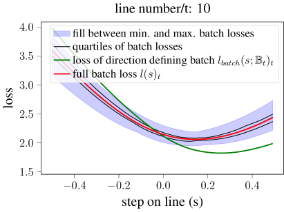
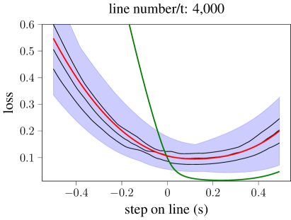
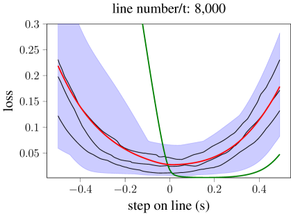
Figure 1: Losses along the lines of the SGD training processes exhibit a parabolic shape. The loss of the direction defining mini-batch (green) is excluded from the distribution of mini-batch losses to show that it is significantly different. This makes line searches on it unfavorable. In addition, the parabolic property articulates stronger for the full-batch loss (red); thus, this work aims to approximate it efficiently with a parabola. This introducing figure is created with code and data from Mutschler & Zell (2021).

Deterministic line searches: According to (Jorge & Stephen, 2006, §3), line searches are considered a solved problem, in the noise-free case. However, such methods are not robust to gradient and loss noise and often fail in this scenario since they shrink the search space inadequately or use too inexact approximations of the loss. (Jorge & Stephen, 2006, §3.5) introduces a deterministic line search using parabolic and cubic approximations of the loss, which motivated our approach.
Line searches on mini-batch and full-batch losses and why to favor the latter. The following motivates the goal of our work to introduce a simple, reasonably fast, and well-performing line-search approach that approximates full-batch loss.
Many exact and inexact line search approaches for Deep Learning are applied on mini-batch losses (Mutschler & Zell, 2020; Berrada et al., 2020; Rolinek & Martius, 2018; Baydin et al., 2018; Vaswani et al., 2019). (Mutschler & Zell, 2020) approximates an exact line search by estimating the minimum of the mini-batch loss along lines with a one-dimensional parabolic approximation. The other approaches perform inexact line searches by estimating positions of the mini-batch loss along lines, which fulfill specific conditions. Such, inter alia, are the Goldberg, Armijo, and Wolfe conditions (see Jorge & Stephen (2006)). For these, convergence on convex stochastic functions can be assured under the interpolation condition (Vaswani et al., 2019), which holds if the gradient with respect to each batch converges to zero at the optimum of the convex function. Under this condition, the convergence rates match those of gradient descent on the full-batch loss for convex functions (Vaswani et al., 2019). However, relying on those assumptions and on mini-batch losses only does not lead to robust optimization, especially not if the gradient noise is high, as will be shown in Section 4. (Mutschler & Zell, 2021; 2020) even showed that exact line searches on mini-batch losses are not working at all. Line searches on the non-stochastic full-batch loss show linear convergence on any deterministic function that is twice continuously differentiable, has a relative minimum, and only positive eigenvalues of the Hessian at the minimum (see Luenberger et al. (1984)). In addition, they are independent of gradient noise. Therefore, it is reasonable to consider line searches on the full-batch loss. However, these are cost-intensive since a massive amount of mini-batch losses for multiple positions along a line must be determined to measure the full-batch loss.
Probabilistic Line Search (PLS) (Mahsereci & Hennig, 2017) addresses this problem by performing Gaussian Process Regressions, which result in multiple one-dimensional cubic splines. In addition, a probabilistic belief over the first (aka Armijo condition) and second Wolfe condition is introduced to find appropriate update positions. The major drawback of this conceptually appealing method is its high complexity and slow training speed. A different approach working on the full-batch loss is Gradient-only line search (GOLSI) (Kafka & Wilke, 2019). It approximates a line search on the full-batch loss by considering consecutive noisy directional derivatives whose noise is considerably smaller than the noise of the mini-batch losses.
Empirical properties of the loss landscape: In Deep Learning, loss landscapes of the true loss (over the whole distribution), the full-batch loss, and the mini-batch loss can, in general, be highly non-convex. However, to efficiently perform a line search, some properties of these losses have to be apparent. Little is known about such properties from a theoretical perspective; however, several works suggest that loss landscapes tend to be simple and have some properties: Mutschler & Zell (2021); Li et al. (2018); Xing et al. (2018); Mutschler & Zell (2020); Chae & Wilke (2019); Mahsereci & Hennig (2017); Goodfellow et al. (2015); Fort & Jastrzebski (2019); Draxler et al. (2018). (Mahsereci & Hennig, 2017; Xing et al., 2018; Mutschler & Zell, 2021; 2020) suggest that the full-batch loss $\mathcal{L}$ along lines in negative gradient directions tend to exhibit a simple shape for a set of Deep Learning problems. This set includes at least classification tasks on CIFAR-10, CIFAR-100, and ImageNet. (Mutschler & Zell, 2021) sampled the full-batch loss along the lines in SGD update step directions. This was done for $10,000$ consecutive SGD and SGD with momentum update steps of a ResNet18’s, ResNet20’s and MobileNetv2’s training process on a subset of CIFAR-10. Representative plots of their $10,000$ measured full-batch losses along lines are presented in Figure 1. Relevant insights and found properties of these works will be introduced and exploited to derive our algorithm in Section 3.
Using the batch size to tackle gradient noise: Besides decreasing the learning rate, increasing the batch size remains an important choice to tackle gradient noise. McCandlish et al. exploits empirical information to predict the largest piratical batch size over datasets and models. De et al. adaptively increases the batch size over update steps to assure that the negative gradient is a descent direction. Smith & Le introduces the noise scale, which controls the magnitude of the random fluctuations of consecutive gradients interpreted as a differential equation. The latter leads to the observation that increasing the batch size has a similar effect as decreasing the learning rate (Smith et al., 2018), which is exploited by our algorithm.

3 Our approach: Large-Batch Parabolic approximation line search (LabPal)

3.1 Mathematical Foundations

In this subsection, we introduce the mathematical background relevant for line searches and challenges that must be solved in order to perform line searches in Deep Learning.
 We consider the problem of minimizing the full-batch loss $\mathcal{L}$, which is the mean over a large amount of sample losses $L_{d}$:

$$\mathcal{L}\;:\;\mathbb{R}^{n}\rightarrow\mathbb{R},\;\mathbf{\theta}\mapsto\frac{1}{|\mathbb{D}|}\sum_{d\in\mathbb{D}}L_{d}(\mathbf{\theta}),$$ (1)

where $\mathbb{D}$ is a finite dataset and $\mathbf{\theta}$ are $n$ parameters to optimize. To increase training speed generally, a mini-batch loss $\mathcal{L}_{\mathbb{B}}$, which is a noisy estimate of $\mathcal{L}$, is considered:

$$\mathcal{L}_{\mathbb{B}}\;:\;\mathbb{R}^{n}\rightarrow\mathbb{R},\;\mathbf{\theta}\mapsto\frac{1}{|\mathbb{B}|}\sum_{d\in\mathbb{B}\subset\mathbb{D}}L_{d}(\mathbf{\theta}),$$ (2)

with $|\mathbb{B}|\ll|\mathbb{D}|$. We define the mini-batch gradient at step $t$ as $\mathbf{g}_{\mathbb{B},t}\in\mathbb{R}^{n}$ as $\nabla_{\mathbf{\theta}_{t}}\mathcal{L}_{\mathbb{B}}(\mathbf{\theta}_{t})$.

For our approach, we need the full-batch loss along the direction of the negative normalized gradient of a specific mini-batch loss. At optimization step $t$ with current parameters $\mathbf{\theta}_{t}$ and a direction defining batch $\mathbb{B}_{t}$, $\mathcal{L}_{\mathbb{B}}$ along a line with origin $\mathbf{\theta}_{t}$ in the negative direction of the normalized batch gradient $\hat{\mathbf{g}}_{\mathbb{B},t}=\nicefrac{{\mathbf{g}_{\mathbb{B},t}}}{{||\mathbf{g}_{\mathbb{B},t}||}}$ is given as:

$$l_{\mathbb{B}{,t}}\;:\;\mathbb{R}\rightarrow\mathbb{R},\;s\mapsto\mathcal{L}_{\mathbb{B}}(\mathbf{\theta}_{t}+s\cdot-\hat{\mathbf{g}}_{\mathbb{B}_{t},t}),$$ (3)

where $s$ is the step size along the line. The corresponding full-batch loss along the same line is given by:

$$l_{t}:\;\mathbb{R}\rightarrow\mathbb{R},\;s\mapsto\mathcal{L}(\mathbf{\theta}_{t}+s\cdot-\hat{\mathbf{g}}_{\mathbb{B}_{t},t}).$$ (4)

Let the step size to the first encountered minimum of $l_{t}$ be $s_{\text{min},t}$.

Two major challenges have to be solved in order to perform line searches on $\mathcal{L}$:

1. To measure $l_{t}$ exactly it is required to determine every $L_{d}(\mathbf{\theta}_{t}+s\cdot-\hat{\mathbf{g}}_{\mathbb{B}_{t},t})$ for all $d\in\mathbb{D}$ and for all step sizes $s$ on a line.

2. To assure convergence line searches have to be performed in a descent direction (De et al., 2016). The simplest form is the direction of steepest descent (Luenberger et al., 1984). Therefore, the full-batch gradient $\nabla_{\mathbf{\theta}}\mathcal{L}\;:\;\mathbb{R}^{n}\rightarrow\mathbb{R}^{n},\;\mathbf{\theta}\mapsto\frac{1}{|\mathbb{D}|}\sum\limits_{d\in\mathbb{D}}\nabla L_{d}(\mathbf{\theta}_{t})$ has to be approximated.

To be efficient, $l_{t}$ has to be approximated sufficiently well with as little data points $d$ and steps $s$ as possible, and one has to use as little $d$ as possible to approximate $\nabla_{\mathbf{\theta}}\mathcal{L}$ approximated sufficiently well. Such approximations are highly dependent on properties of $\mathcal{L}$. Due to the complex structure of Deep Neural Networks, little is known about such properties from a theoretical perspective. Thus, we fall back to empirical properties.

3.2 Deriving the algorithm

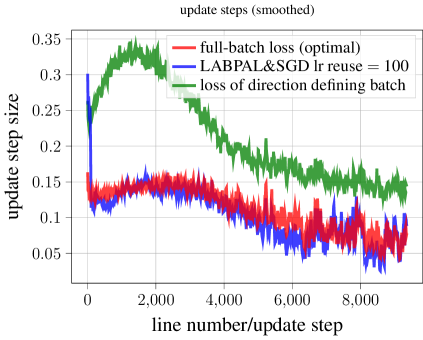
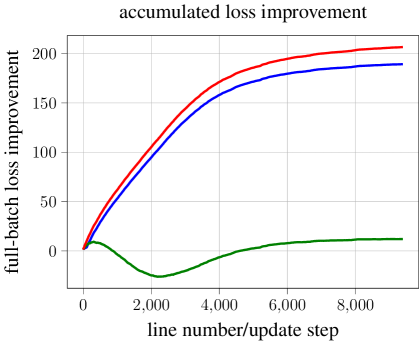
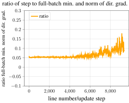
Figure 2: Several metrics to compare update step strategies on the full-batch losses along 10,000 lines measured by Mutschler & Zell (2021): 1. update step sizes, 2. accumulated loss improvement per step given as: $l(0)-l(s_{upd})$ where $s_{upd}$ is the update step of a specific optimizer. This is the locally optimal improvement to the minimum of the full-batch loss along a line. The right plot shows almost proportional behavior between the optimal update step and the negative gradient norm of the direction defining mini-batch loss. The LABPAL&SGD version of our approach performs almost optimal on ground truth data. Results LABPAL&NSGD are almost identical and thus omitted. Plotting code based on Mutschler & Zell (2021) with addition of our proposed approach.

Algorithm 1 LABPAL&SGD. Simplified conceptional pseudo-code of our proposed algorithm, which estimates update steps on a parabolic approximation of the full-batch loss. See the published source code for technical details. Default values are given in parenthesis. For LABPAL&NSGD SGD is replaced with NSGD, and the update step is measured instead of the learning rate.

0:  Hyperparameters: - initial parameters $\theta_{0}$- approximation batch size $|\mathbb{B}_{a}|$ $(1280)$- inference batch size $|\mathbb{B}_{i}|$ $(128)$- SGD steps $n_{\text{SGD}}$ $(1000)$,  # or NSGD steps- step size adaptation $\alpha>1$ $(1.8)$- training steps $t_{max}(150000)$ - batch size schedule $k(t)=\begin{cases}1,&\text{if $t\leq\lfloor t_{max}\cdot 0.5\rfloor$}\\ 2,&\text{elif $t\leq\lfloor t_{max}\cdot 0.75\rfloor$}\\ 4,&\text{elif $t>\lfloor t_{max}\cdot 0.75\rfloor$}\end{cases}$

1:  # Variables have global scope

2:  sampledBatchSize $\leftarrow 0$

3:  performedSGDsteps $\leftarrow$ 0

4:  learningRate $\leftarrow$ 0

5:  $\theta\leftarrow\theta_{0}$

6:  state $\leftarrow$ ’line search’

7:  direction $\leftarrow$ current batch gradient

8:  $t\leftarrow 0$

9:  while $t<t_{max}$ do

10:     if state is ’line search’ then

11:        perform_line_search_step()

12:     end if

13:     if state is ’SGDTraining’ then

14:        perfrom_large_batch_sgd_step()

15:     end if

16:  end while

17:  return  $\theta$

18:  procedure perform_line_search_step()

19:     if sampledBatchSize $<|\mathbb{B}_{a}|$  then

20:        update estimate $\hat{\mathcal{L}}$ of $\mathcal{L}$ withover multiple inferences sampled $\mathcal{L}_{\mathbb{B}_{t},t}$ with $|\mathbb{B}_{t}|=k(t)\cdot|\mathbb{B}_{i}|)$

21:        increase sampledBatchSize by $|\mathbb{B}_{t}|$ and $t$ by $k(t)$

22:     else

23:        learningRate $\leftarrow$ perform parabolic approximation with 3 values of $\hat{\mathcal{L}}$ along the search direction and estimate the learning rate.

24:        learningRate $\leftarrow$ learningRate $\cdot\alpha$

25:        set sampledBatchSize and performedSGDsteps to $0$

26:        state $\leftarrow$ ’SGDTraining’

27:     end if

28:  end procedure

29:  

30:  procedure perfrom_large_batch_sgd_step()

31:     if performedSGDsteps $<n_{\text{SGD}}$ then

32:        $\theta$ $\leftarrow$ perform SGD update with learningRate and over multiple inferences sampled $\mathcal{L}_{\mathbb{B}_{t},t}$ with $|\mathbb{B}_{t}|=k(t)\cdot|\mathbb{B}_{i}|)$

33:        increase $t$ by $k(t)$

34:        increase performedSGDsteps by $1$

35:     else

36:        direction $\leftarrow$ current batch gradient

37:        state $\leftarrow$ ’line search’

38:     end if

39:  end procedure

In the following, we derive our line search approach on the full-batch loss by iteratively exploiting empirically found observations of (Mutschler & Zell, 2021) and solving the challenges for a line search on the full-batch loss (see Section 3.1). Given default values are inferred from a detailed hyper parameter analysis (Section A)
Observation 1: Minima of $l_{\mathbb{B}{,t}}$ can be at significantly different points than minima of $l_{t}$ and can even lead to update steps, which increase $\mathcal{L}$ (Figure 2 center, green and red curve).
Derivation Step 1: This consolidates that line searches on a too low mini-batch loss are unpromising. Consequently, we concentrate on a better way to approximate $l_{t}$.
Observation 2: $l_{t}$ can be approximated with parabolas of positive curvature, whose fitting errors are of less than $0.6\cdot 10^{-2}$ mean absolute distance (exemplarily shown in Figure 1).
Derivation Step 2: We approximate $l_{t}$ with a parabola ($l(s)_{t}\approx a_{t}s^{2}+b_{t}s+c_{t}$ with $a_{t}>0$). A parabolic approximation needs three measurements of $l_{t}$. However, already computing $l_{t}$ for one $s$ only is computationally unfeasible. Assuming i.i.d sample losses, the standard error of $l_{\mathbb{B}{,t}}(s)$, decreases with $\nicefrac{{1}}{{\sqrt{|\mathbb{B}|}}}$. Thus, $l_{\mathbb{B}{,t}}$ -with a reasonable large batch size- is already a good estimator for the full-batch loss parabola. Consequently, we approximate $l_{t}$ with $l_{\mathbb{B}_{a},t}$ by averaging over multiple $l_{\mathbb{B}_{i},t}$ measured with multiple inferences. Thus, the approximation batch size $\mathbb{B}_{a}$, is significantly larger as the, by GPU memory limited, possible batch size $\mathbb{B}_{i}$. In our experiments, $\mathbb{B}_{a}$ is usually chosen to be $1280$, which is $10$ times larger as $\mathbb{B}_{i}$. In detail, we measure $l_{\mathbb{B}_{a},t}$ at the points $s=0,0.0001$ and $0.01$, then we simply infer the parabola’s parameters and the update step to the minimum. These values of $s$ empirically lead to the best and numerically most stable approximations.
Observation 3: The trend of $s_{\text{min},t}$ of consecutive $l_{t}$ changes slowly and consecutive $l_{t}$ do not change locally significantly. (Figure 2 left, red curve).
Observation 4: $s_{\text{min},t}$ and the direction defining batch’s $||\mathbf{g}_{\mathbb{B}_{t},t}||$ are almost proportional during training. (Figure 2 right).
Derivation Step 3: Using measurements of $l_{\mathbb{B}_{a},t}$ to approximate $l_{t}$ with a parabola is by far to slow to compete against SGD if done for each weight update. By exploiting Observation 3 we can approximate $l_{t}$ after a constant amount of steps and reuse the measured learning rate $\lambda$ or update step size $s_{\text{upd}}$ for subsequent steps. In this case, $\lambda$ is a factor multiplied by $\mathbf{g}_{\mathbb{B},t}$, whereas $s_{\text{upd}}$ is a factor multiplied by $\hat{\mathbf{g}}_{\mathbb{B},t}$. Consequently with $\lambda$ we perform a step in gradient direction (as SGD also does), whereas, with $s_{\text{upd}}$ we perform a step in normalized gradient direction, ignoring the norm of the gradient. Observation 4 allows us to reuse $\lambda$. In our experiments, it is sufficient to measure a new $\lambda$ or $s_{\text{upd}}$ every 1000 steps only.
Derivation Step 4: So far, we can approximate $l_{t}$ efficiently and, thus, overcome the first challenge (see Section 3.1). Now, we will overcome the second challenge; approximating the full batch loss gradient for each weight update step:
For this, we revisit Smith et al. (2018) who approximates the magnitude of random gradient fluctuations, that appear if training with a mini-batch gradient, by the noise scale $\nu\in\mathbb{R}$:

$$\nu\approx\nicefrac{{(\lambda|\mathbb{D}|)}}{{|\mathbb{B}|}},$$ (5)

where $\lambda$ is the learning rate, $|\mathbb{D}|$ the dataset size and $|\mathbb{B}|$ the batch size. If the random gradient fluctuations are reduced, the approximation of the gradient gets better. Since we want to estimate the learning rate automatically, the only tunable parameter to reduce the noise scale is the batch size.
Observation 5: The variance of consecutive $s_{\text{min},t}$ is low, however, it increases continuously during training (Figure 2 left, red curve).
Derivation Step 5: It stands to reason that the latter happens because the random gradient fluctuations increase. Consequently, during training, we increase the batch size for weight updates by iteratively sampling a larger batch with multiple inferences. This reduces the variance of consecutive $s_{\text{min},t}$ and lets us reuse estimated the $\lambda$ or $s_{\text{upd}}$ for more steps. After experiencing unusable results with the approach of (De et al., 2016) to determine appropriate batch sizes, we stick to a simple piece-wise constant batch size schedule doubling the batch size after two and after three-quarters of the training.
Observation 6: On a global perspective a $s_{\text{upd}}$ that overestimates $s_{\text{min},t}$ optimizes and generalizes better.
Derivation Step 6: Thus, after estimating $\lambda$ (or $s_{\text{min}}$) we multiply it with a factor $\alpha\in]1,2[$:

$$\lambda_{\text{new}}=\alpha\lambda=\nicefrac{{\alpha s_{\text{min},t}}}{{||\mathbf{g}_{\mathbb{B},t}||}}\quad\text{or}\quad s_{\text{upd}}=\alpha s_{\text{min},t}$$ (6)

Note that under out parabolic property, the first wolfe condition $w_{1}$, which is commonly used for line searches, simply relates to $\alpha$: $w_{1}=-\frac{\alpha}{2}+1$ (see Appendix F).

Combining all derivations leads to our line search named large-batch parabolic approximation line search (LABPAL), which is given in Algorithm 1. It samples the desired batch size over multiple inferences to perform a close approximation of the full-batch loss and then reuses the estimated learning rate to train with SGD (LABPAL&SGD), or it reuses the update step to train with SGD with a normalized gradient (LABPAL&NSGD). While LABPAL&SGD elaborates Observation 4, LABPAL&NSGD completely ignores information from $||\mathbf{g}||$.

4 Empirical Analysis

Our two approaches are compared against other line search methods across several datasets and networks in the following. To reasonably compare different line search methods, we define a step as the sampling of a new input batch. Consequently, the steps/batches that LABPAL takes to estimate a new learning rate/step size are considered, and optimization processes are compared on their data efficiency.
Note that the base ideas of the introduced line search approaches can be applied upon any direction giving technique such as Momentum, Adagrad (Duchi et al., 2011) or Adam (Kingma & Ba, 2015). Results are averaged over 3 runs.

4.1 Performance analysis on ground truth full-batch loss and proof of concept

 
 

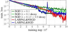
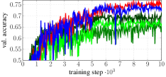
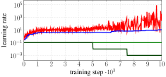
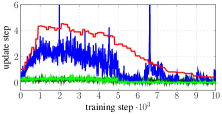
Figure 3: Training process on the problem of which the empirical observations were inferred ( ResNet-20 trained on 8% of CIFAR-10 with SGD). LABPAL&NSGD and LABPAL&SGD outperform SGD. Interestingly LABPAL&NSGD estimated huge $\lambda$s, whereas $s_{upd}$s are decreasing

To analyze how well our approach approximates the full-batch loss along lines, we extended the experiments of Mutschler & Zell (2021) by LABPAL. Mutschler & Zell (2021) measured the full-batch loss along lines in SGD update step directions of a training process; thus, this data provides ground truth to test how well the approach approximates the full-batch loss. In this scenario, LABPAL&SGD uses the full-batch size to estimate the learning rate and reuses it for 100 steps. No update step adaptation is applied. Figure 2 shows that LABPAL&SGD fits the update step sizes to the minimum of the full-batch loss and performs near-optimal local improvement. The same holds for LABPAL&NSGD.
We now test how our approaches perform in a scenario for which we can assure that the used empirical observations hold. Therefore, we consider the optimization problem of (Mutschler & Zell, 2021) from which all empirical observations were inferred, which is training a ResNet20 on 8% of CIFAR10. $\mathbb{B}_{a}$ of 1280 is used for both approaches. Learning rates are reused for 100 steps, and $\alpha=1.8$ is considered. The batch size is doubled after $5000$ and $7500$ steps. For SGD $\lambda$ is halved after the same steps. A grid search for the best $\lambda$ is performed. Figure 3 shows that LABPAL&NSGD with update step adaptation outperforms SGD, even though $9\%$ of the training steps are used to estimate new update step sizes. This shows that using the estimated learning rates and step sizes leads to better performance than keeping them constant or decaying them with a piece-wise schedule. Interestingly huge $\lambda$s of up to $80,000$ are estimated, whereas $s_{\text{upd}}$s are decreasing. LABPAL&SGD shows similar performance as SGD; however, it seems beneficial to ignore gradient size information as the better performance of LABPAL&NSGD shows.

4.2 Performance comparison to SGD and to other line search approaches

We compare the SGD and NSGD variants of our approach against PLS (Mahsereci & Hennig, 2017), GOLSI (Kafka & Wilke, 2019), PAL (Mutschler & Zell, 2020), SLS (Vaswani et al., 2019) and SGD with Momentum (Robbins & Monro, 1951). The latter is a commonly used optimizer for Deep Learning problems and can be reinterpreted as a parabolic approximation line search on mini-batch losses (Mutschler & Zell, 2021). PLS is of interest since it approximates the full-batch loss to perform line searches. PAL, GOLSI, SLS on the other hand are line searches optimizing on mini-batch losses directly. For SGD with Momentum, a piece-wise constant learning rate schedule divides the learning rate after two and again after three-quarters of the training by a factor of 10.

Comparison is done across several datasets and models. Specifically, we compare ResNet-20 (He et al., 2016), DenseNet-40 (Huang et al., 2017), and MobileNetV2 (Sandler et al., 2018) trained on CIFAR-10 (Krizhevsky & Hinton, 2009a), CIFAR-100 (Krizhevsky & Hinton, 2009b), and SVHN (Netzer et al., 2011). We concentrate on classification problems since the empirical observations are inferred from a classification task and since those problems are usually considered to benchmark new optimization approaches.

For each optimizer, we perform a comprehensive hyper-parameter grid search on ResNet-20 trained on CIFAR-10 (see Appendix G.1). The best performing hyper-parameters on the validation set are then reused for all other experiments. The latter is done to check the robustness of the optimizer by handling all other datasets as if they were unknown, as is usually the case in practice. Our aim here is to show that satisfactory results can be achieved on new problems without any fine-tuning needed. Further experimental details are found in Appendix G.

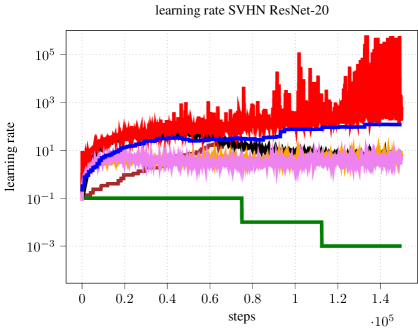
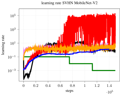
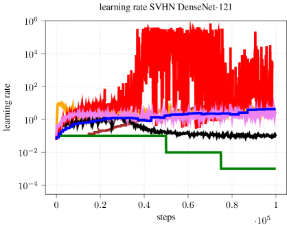
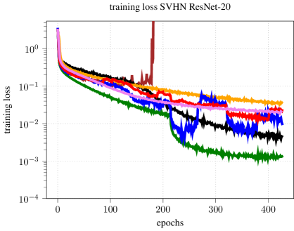
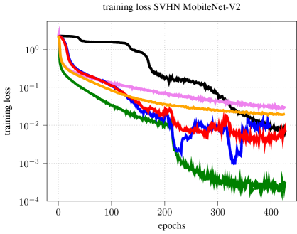
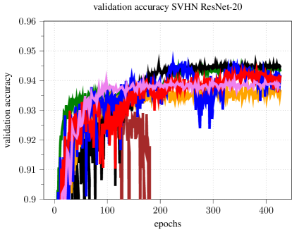
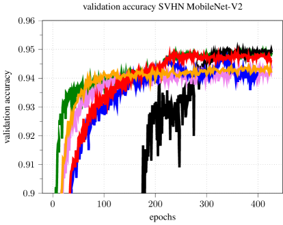
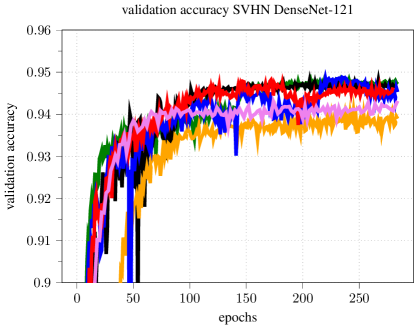
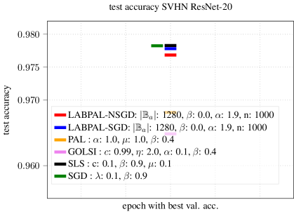
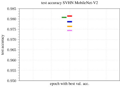
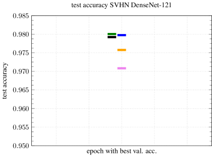
Figure 9: Performance comparison on SVHN of our approach LABPAL in the SGD and NSGD variants against several line search and SGD. Optimal hyperparameters found with a detailed grid search for CIFAR-10 are reused. Our approaches challenge and sometimes surpass the other approaches on training loss, validation, and test accuracy. Columns indicate different models. Rows indicate different metrics.

Figure 4 as well as Appendix Figures 8, 9 show that both LABPAL approaches outperform PLS, GOLSI and PAL considering training loss, validation accuracy, and test accuracy. LABPAL&NSGD tends to perform more robust and better than LABPAL&SGD. LABPAL&NSGD is on pair with SGD with Momentum and challenges SLS on validation and test accuracy. The important result is that hyper-parameter tuning for LABPAL is not needed to achieve good results across several models and datasets. However, this also is true for pure SGD, which suggests that the simple rule of performing a step size proportional to the norm of the momentum term is sufficient to implement a well-performing line search. This also strengthens the observation of (Mutschler & Zell, 2021), which states that SGD, with the correct learning rate, is already performing an almost optimal line search.

The derived learning rate schedules of the LABPAL approaches are significantly different from a piece-wise constant schedule (Figure 4, 8, 9 first row). Interestingly they show a strong warm up (increasing) phase at the beginning of the training followed by a rather constant phase which can show minor learning rate changes with an increasing trend. The NSGD variant sometimes shows a second increasing phase, when the batch size is changed. The warm up phase is often seen in sophisticated learning rate schedules for SGD; however, usually combined with a cool down phase. The latter is not apparent for LABPAL since we increase the batch size. LABPAL&NSGD indirectly uses learning rates of up to $10^{6}$ but still trains robustly. Of further interest is that all line search approaches do not decrease the learning rate at the end of the training as significantly as SGD, which hinders the line searches to converge.

A comparison of training speed and memory consumption is given in Appendix D. In short, LABPAL has identical GPU memory consumption as SGD and is on average only $19.6\%$ slower. However, for SGD usually a grid search is needed to find a good $\lambda$, which makes LABPAL considerably cheap.

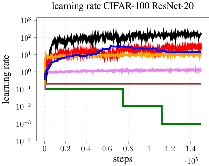
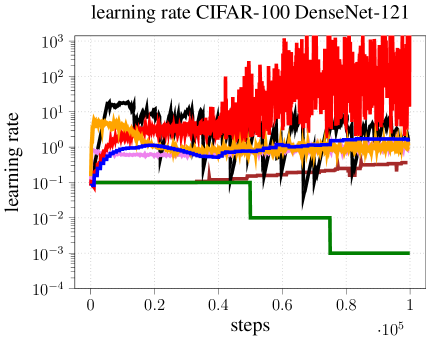
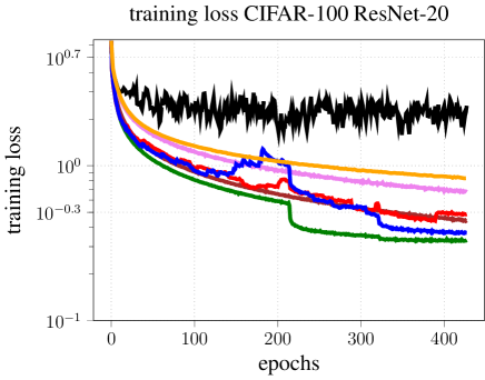
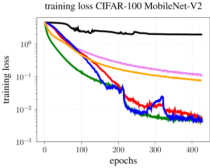
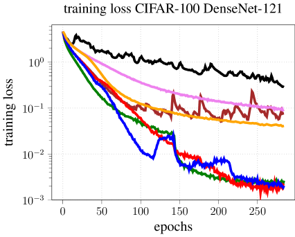
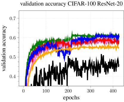
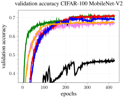
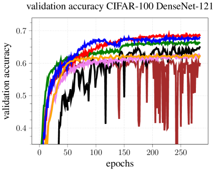
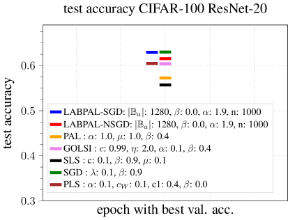
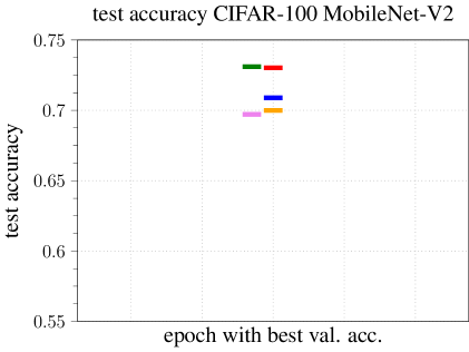
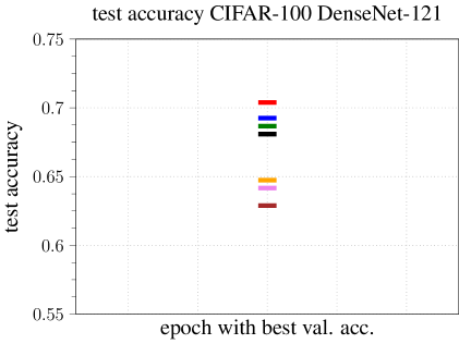
Figure 4: Performance comparison on CIFAR-100 of our approach LABPAL in the SGD and NSGD variants against several line searches and SGD with momentum. Optimal hyperparameters for CIFAR-10 ResNet-20 found with a grid search are reused (Appendix G.1). Here, our approaches surpass the other approaches on training loss, validation, and test accuracy. Columns indicate different models. Rows indicate different metrics. Results for CIFAR-10 and SVHN are given in appendix Figures 8, and 9. The batch-size used is $128$. Due to a too high memory consumption we could not run PLS on MobileNet-V2.

4.3 Adaptation to varying gradient noise

Recent literature, E.g., (Mutschler & Zell, 2020), (Vaswani et al., 2019), (Kafka & Wilke, 2019) show that line searches work with a relatively large batch size of 128 and a training set size of approximately 40000 on CIFAR-10. However, a major, yet not comprehensively considered problem is that line searches operating on the mini-batch loss vary their behavior with another batch- and training set sizes leading to varying gradient noise. E.g., Figure 5 shows that training with PAL, GOLSI or PlS and a batch size of 8 on CIFAR-10 does not work at all. The reason is that the by mini-batches induced gradient noise, and with it the difference between the full-batch loss and the mini-batch loss, increases. However, we can adapt LABPAL to work in these scenarios by holding the noise scale it is exposed to approximately constant. As the learning rate is inferred directly, the batch size has to be adapted. Based on the linear approximation of the noise scale (see Equation 5), we directly estimate a noise adaptation factor $\epsilon\in\mathbb{R}$ to adapt LABPAL’s hyperparameter:

$$\epsilon:=\frac{\nu_{new}}{\nu_{ori}}=\frac{|\mathbb{B}_{ori}|}{|\mathbb{B}_{new}|}\frac{|\mathbb{D}_{new}|}{|\mathbb{D}_{ori}|}=\frac{128}{|\mathbb{B}_{new}|}\frac{|\mathbb{D}_{new}|}{40,000}$$ (7)

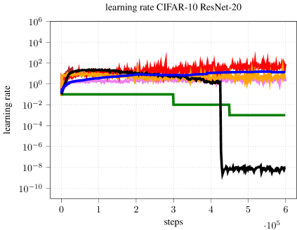
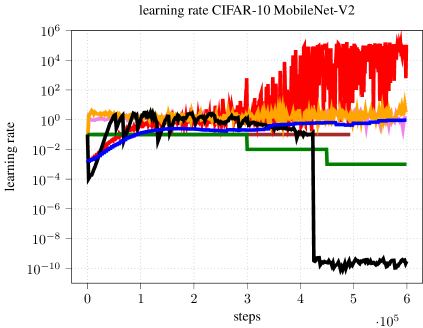
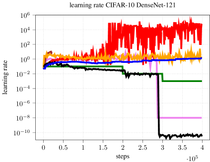
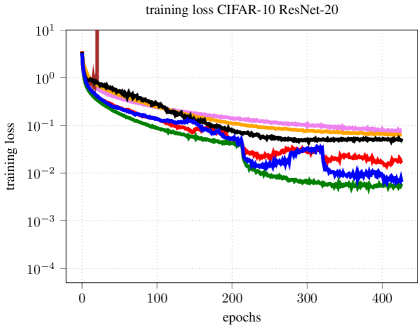
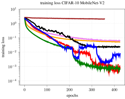
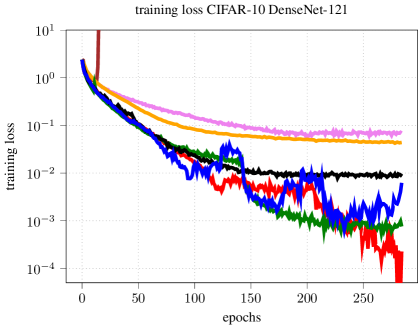
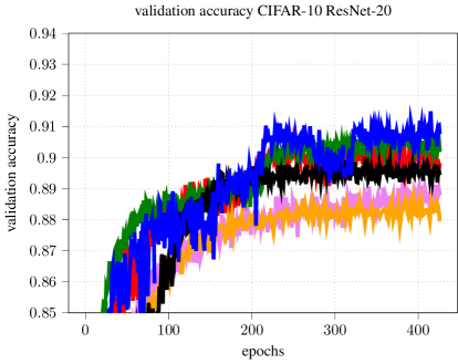
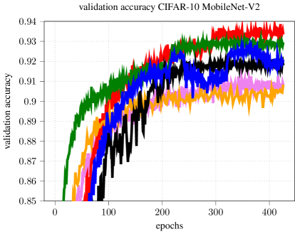
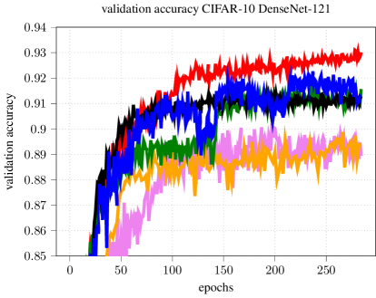
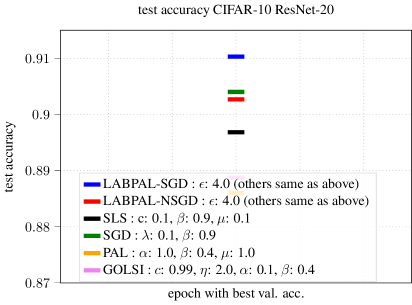
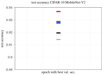
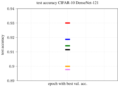
Figure 10: Performance comparison of several models on CIFAR-10 with batch size 32. The same hyperparameters are used as for batch size 128 (see Figure 8). Due to the batch size adaptation to keep the noise scale on a similar level the LABPAL approaches perform almost identical compared to batch size 128. The performance off all other line searches decreases; SGD still performs well. Not that training steps were increased by a factor of 4.

The original batch size $|\mathbb{B}_{ori}|$ and the original dataset size $|\mathbb{D}_{ori}|$ originate from our search for best-performing hyperparameters on CIFAR-10 with a training set size of 40,000, a batch size of 128, and 150,000 training steps. We set the number of training steps to $150,000\epsilon$ and multiply the batch sizes in the batch size schedule $k$ by $\epsilon$. This rule makes the approach fully parameter less in practice (at least for the image classification scenario), since hyperparameters do not have to be adapted across models, batch sizes and datasets. Figure 5 shows a performance comparison over different batch sizes. Hyperparameters are not changed. By changing the batch size the noise adaptation factor of the LABPAL approaches gets adapted, which lets them still perform well with low batch sizes since they iteratively sample larger batch sizes over multiple inferences. The performance of PLS, PAL and GOLSI decreases with lower batch size. SLS’s performance stays similar but its learning rate schedule degenerates. For the evaluation on ResNet-20 and MobileNet-V2 see Appendix Figure 10 & 11. We note that this batch size adaptation approach to keep the noise scale on a similar level could also be applied to all other line searches, however this will exceed the limits of this work.

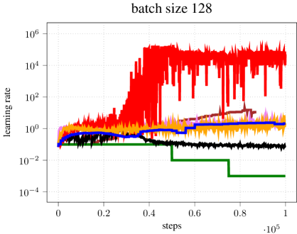
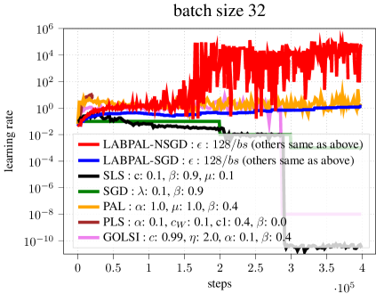
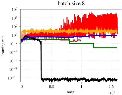
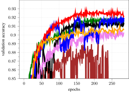
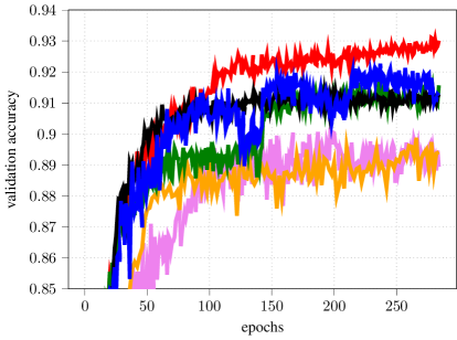
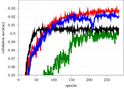
Figure 5: Performance comparison of a DenseNet-121, trained on CIFAR-10 for batch sizes 128, 32 and 8. Hyperparameters are not changed. (For the evaluation on ResNet-20 and MobileNet-V2 see Appendix Figure 10 & 11). PLS curves are incomplete since training failed. Training steps are increased by a factor of 4 and 16 for batch size 32 and 8 respectively.

4.4 Hyperparameter Sensitivity Analysis

We performed a detailed hyperparameter sensitivity analysis for LABPAL&SGD and LABPAL&NSGD. To keep the calculation cost feasible, we investigated the influence of each hyperparameter, keeping all other hyperparameters fixed to the default values (see Algorithm 1). Appendix Figure 6 and 7 show the following characteristics: Estimating new $s_{\text{upd}}$ or $\lambda$ with $\mathbb{B}_{a}$ smaller than $640$ decreases the performance since $l_{t}$ is not fitted well enough (row 1). The performance also decreases if reusing the $\lambda$ (or $s_{\text{upd}}$) for more update steps (row 2), and if using a step size adaptation $\alpha$ of less than 1.8 (row 3, except for ResNet). This shows that optimizing for the locally optimal minimum in line direction is not beneficial. From a global perspective, a slight decrease of the loss by performing steps to the other side of the parabola shows more promise. Interestingly, even using $\alpha$ larger than two still leads to good results. (Mutschler & Zell, 2021) showed that the loss valley in line direction becomes wider during training. This might be a reason why these update steps, which should actually increase the loss, work. Using a maximal step size of less than 1.5 (row 7) and increasing the noise adaptation factor $\epsilon$ (row 9) while keeping the batch size constant also decreases the performance. The latter indicates that the inherent noise of SGD is essential for optimization. In addition, we considered a momentum factor and conclude that a value between $0.4$ and $0.6$ increases the performance for both LABPAL approaches (row 5).

5 Limitations

Our approach can only work if the empirically found properties we rely on are apparent or are still a well enough approximation. In Section 4.2 we showed that this is valid for classification tasks. In additional sample experiments, we observed that our approach also works on regression tasks using the square loss. However, it tends to fail if different kinds of losses from significantly different heads of a model are added, as it is often the case for object detection and object segmentation.

A theoretical analysis is lacking since the optimization field still does not know the reason for the local parabolic behavior of $l_{t}$ is, and consequently, what an appropriate function space to consider for convergence is.

6 Discussion & Outlook

This work introduced a robust line search approach for Deep Learning problems based upon empirically found properties of the full-batch loss. Our approach estimates learning rates well across models, datasets, and batch sizes. It mostly surpasses other line search approaches and challenges SGD with Momentum tuned with a piece-wise constant learning rate schedule. We are the first line search work that analyses and adapts to varying gradient noise. In addition, we show that mini-batch gradient norm information is not necessary for training. In future, we will analyze the causes for the local parabolic behavior of the full-batch loss along lines, to get a better understanding of DNN loss landscapes and especially of why and when specific optimization approaches work.

Reproducibility

Experimental details including all hyperparameters used for the experiments presented in Section 4 are found in App. G.1. The source code to reproduce our experiments including our implementations of SLS, GOLSI, PLS, PAL and LABPAL is provided in the supplementary materials.

Ethics Statement

Since we understand our work as basic research, it is extremely error-prone to estimate its specific ethical aspects and future positive or negative social consequences. As optimization research influences the whole field of deep learning, we refer to the following works, which discuss the ethical aspects and social consequences of AI and Deep Learning in a comprehensive and general way:Yudkowsky et al. (2008); Muehlhauser & Helm (2012); Bostrom & Yudkowsky (2014).

Appendix A Hyperparamter Sensitivity Analysis

.

ResNet-20	MobileNet-V2	DenseNet-121

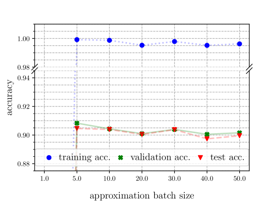
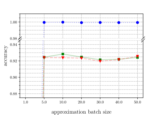
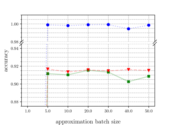
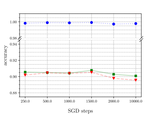
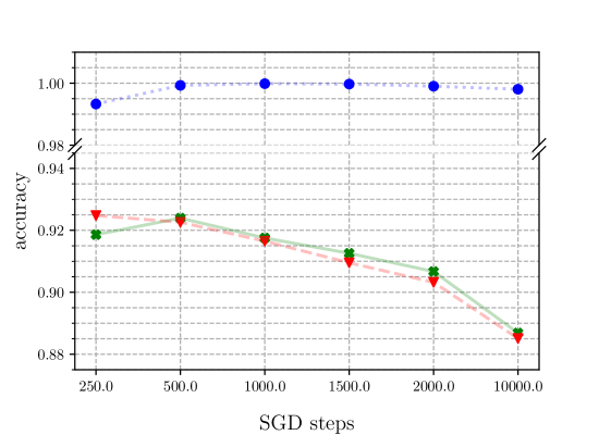
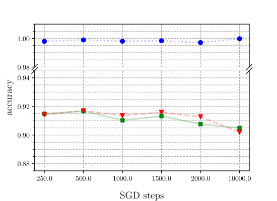
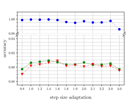
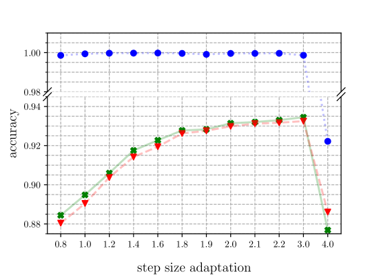
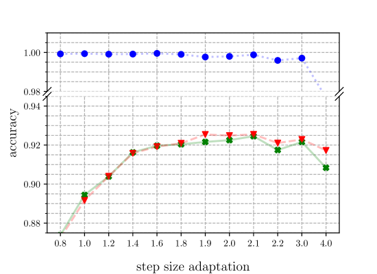
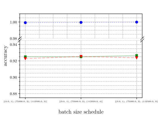
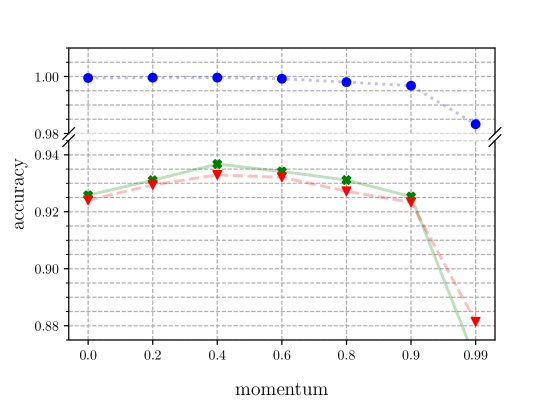
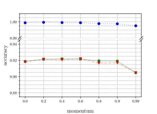
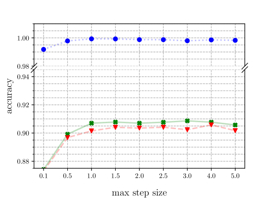
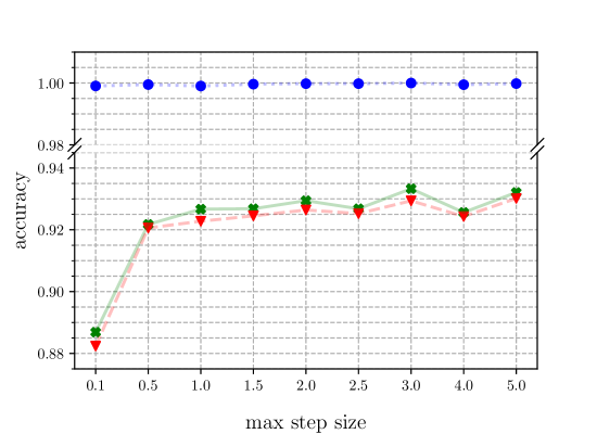
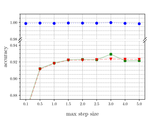
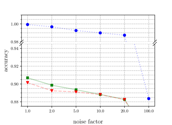
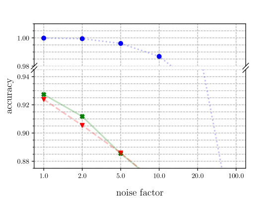
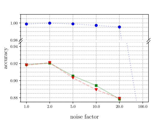
Figure 6: Sensitivity analysis of parameters of LABPAL&SGD. The observations of LABPAL&NSGD described in Figure 7 are also valid for LABPAL&NSGD.

ResNet-20	MobileNet-V2	DenseNet-121

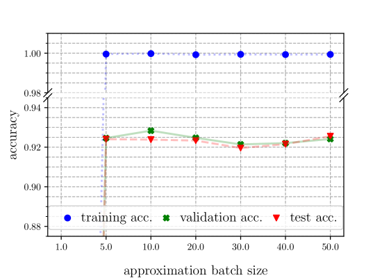
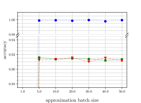
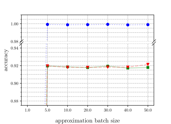
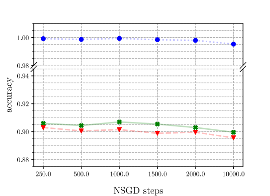
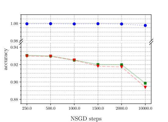
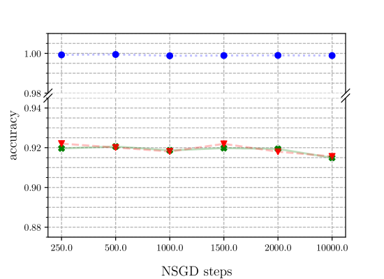
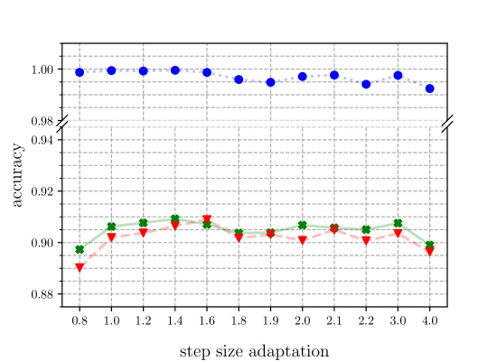
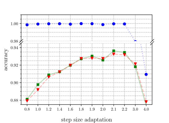
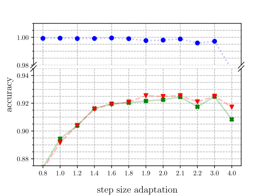
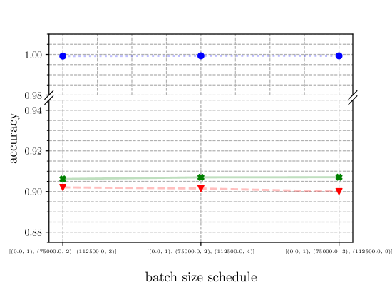
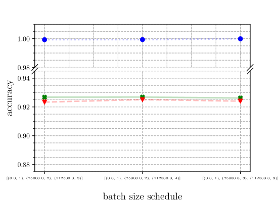
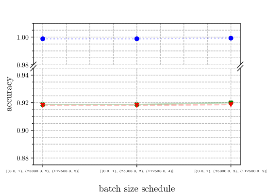
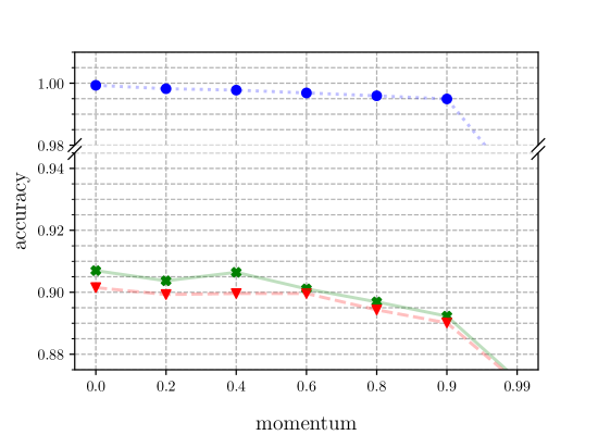
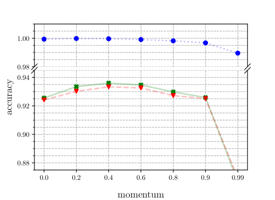
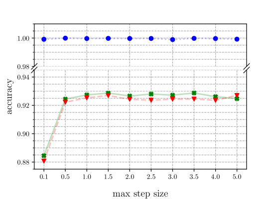
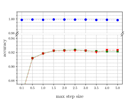
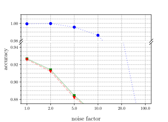
Figure 7: Sensitivity analysis of parameters of LABPAL&NSGD. The default parameters are: approximation batch size $\mathbb{B}_{a}=1280$, SGD steps $s=1000$, step size adaptation $\alpha=1.8$, batch size schedule $k=$ (0:1, 75000:2, 112500:4), momentum $\beta=0$, maximal step size $=1.0$, noise-factor $\epsilon=1$. For $\mathbb{B}_{a}$ the factor 128 is multiplied with is given on the x axis.

Appendix B Further performance comparisons

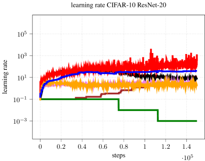
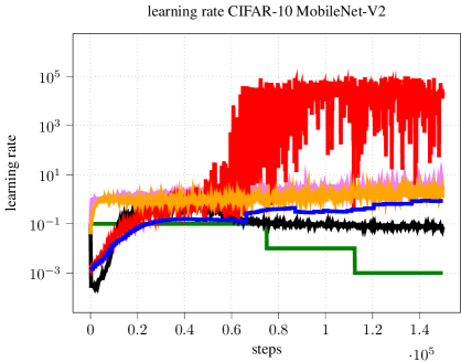
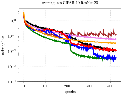
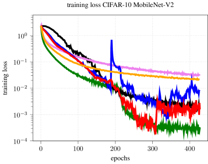
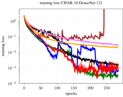
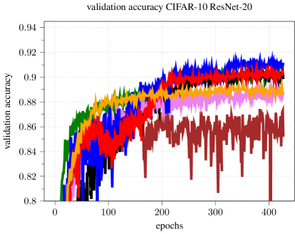
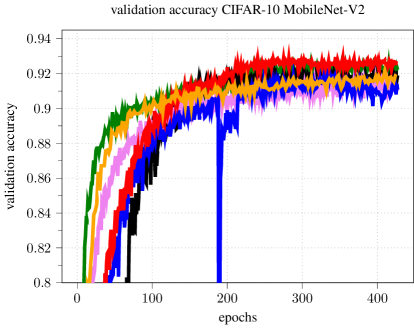
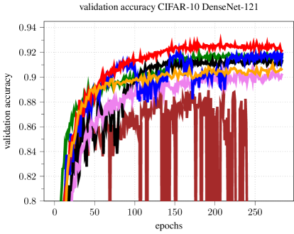
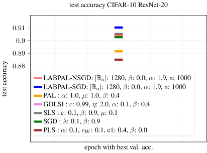
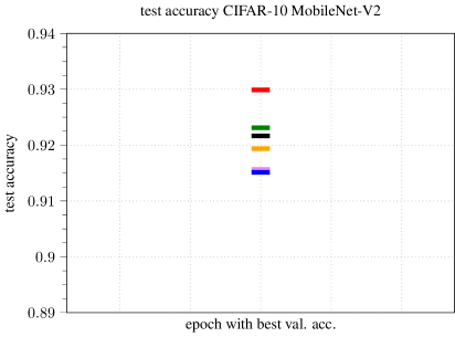
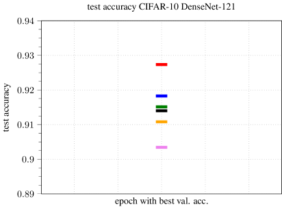
Figure 8: Performance comparison on CIFAR-10 of our approach LABPAL in the SGD and NSGD variants against several line searches and SGD. Optimal hyperparameters are found with an elaborate grid search. Our approaches challenge and sometimes outperform the other approaches on training loss, validation, and test accuracy. Columns indicate different models. Rows indicate different metrics.

Appendix C Further results for batch sizes 32 and 8

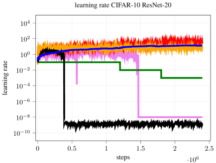
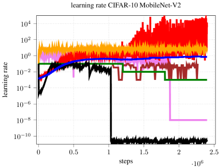
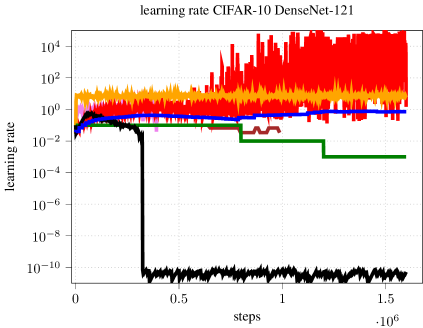
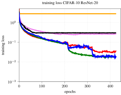
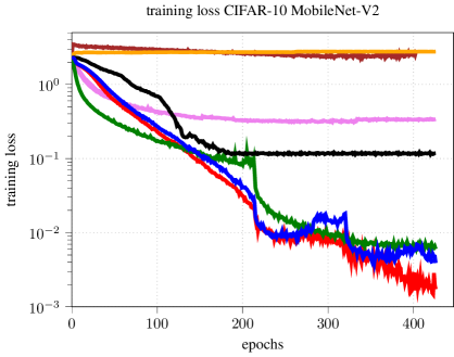
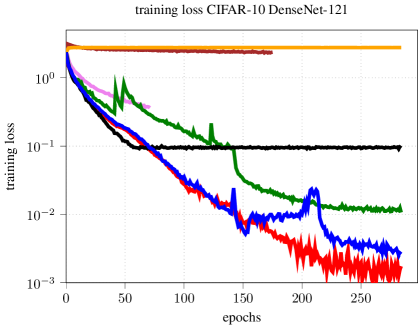
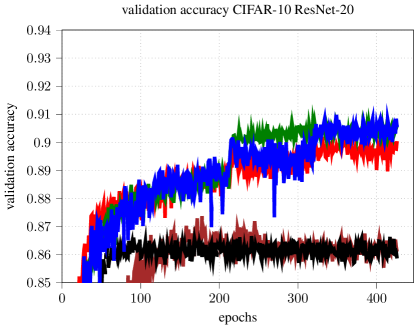
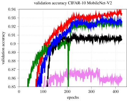
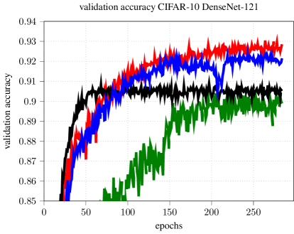
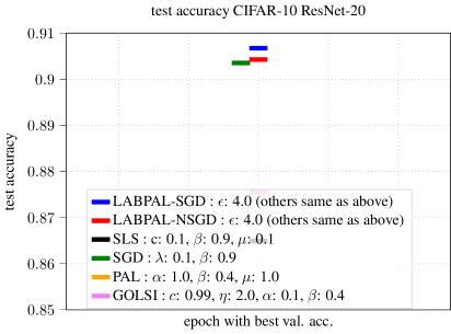
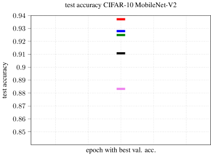
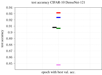
Figure 11: Performance comparison of several models on CIFAR-10 with batch size 8. The same hyperparameters are used as for batch size 128 (see Figure 8). Due to the batch size adaptation to keep the noise scale on a similar level the LABPAL approaches still perform well. PAL and PLS fail to optimize at all. SGD still performs well. SLS still shows good performance, however if training longer this will not hold since the learning rate schedules degenerated. Note that training steps were increased by a factor of 16.

Appendix D Wall clock time and GPU memory comparison

         

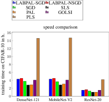
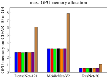
Figure 12: Left: Training time comparison on CIFAR-10. SGD, SLS, and PAL show similar training times. GOLSI, and both variants of LABPAL are slightly slower (up to 19.6%). However, a slightly longer training time is acceptable if less time has to be spent in hyper-parameter tuning. PLS is significantly slower. Note that in comparison to SGD, the implementations of the other optimizers are not optimized on CUDA level. Right: Maximum allocated memory comparison on CIFAR-10. Except for PLS all approaches need approximately the same amount of memory.

Appendix E Theoretical considerations

As the field does not know what the reason for the local parabolic behavior of the full-batch loss is and, thus, what an appropriate function space to consider for convergence is, we refer to the theoretical analysis of (Mutschler & Zell, 2020). They show convergence on a quadratic loss. This is also valid for LABPAL, with the addition that each mini batch-loss can be of any form as long as the mean over these losses is a quadratic function.

Appendix F Relation of update step adaptation $\alpha$ and the first wolfe constant $w_{1}$.

Let $f\;:\;\mathbb{R}\rightarrow\mathbb{R}$ be of form $x\mapsto ay^{2}+by+c$. We start with the first Wolfe condition (a.k.a. Armijo condition, sufficient decrease condition):

$$f(x_{0}+y) \leq f(x_{0})-y\nabla f(x_{0})w_{1} \text{in our case }x_{0}=0,w_{1}\text{ wolfe constant}$$ (8)

$$f(y) \leq f(0)+ybw_{1}$$ (9)

$$ay^{2}+by+c \leq c+ybw_{1} \text{use quadratic shape},\nabla f(x_{0})=b$$ (10)

$$ay^{2}+by-ybw_{1} \stackrel{{\scriptstyle!}}{{=}}0$$ (11)

$$\frac{ay^{2}+by}{by} =\frac{ay}{b}+1=w_{1}$$ (12)

$$-\frac{\alpha}{2}+1 =w_{1} \text{set }y=\alpha\frac{-b}{2a},\alpha\in[1,2)$$ (13)

$$-2w_{1}+2 =\alpha$$ (14)

Appendix G Further experimental details

Further experimental details for the optimizer comparison in Figure 8,4,9,LABEL:labpal_fig_performance_comp_batch_size10,LABEL:labpal_fig_opt_comparison_bs10_same,LABEL:labpal_fig_opt_comparison_bs10_best of Sections 4.2 & 4.3.

PLS: We adapted the only available and empirically improved TensorFlow (Abadi et al., 2015) implementation of PLS (Balles, 2017), which was transferred to PyTorch (Paszke et al., 2019) by (Vaswani et al., 2019), to run on several state-of-the-art models and datasets.

The training steps for the experiments in section Section 4 were 100,000 for DenseNet and 150,000 steps for MobileNetv2 and ResNet-20. Note that we define one training step as processing one input batch to keep line search approaches comparable.

The batch size was 128 for all experiments. The validation/train set splits were: 5,000/45,000 for CIFAR-10 and CIFAR-100 20,000/45,000 for SVHN.

All images were normalized with a mean and standard deviation determined over the dataset. We used random horizontal flips and random cropping of size 32. The padding of the random crop was 8 for CIFAR-100 and 4 for SVHN and CIFAR-10.

All trainings were performed on Nvidia Geforce 1080-TI GPUs.

Results were averaged over three runs initialized with three different seeds for each experiment.

For implementation details, refer to the source code provided at
https://github.com/cogsys-tuebingen/LABPAL.

G.1 Hyperparameter grid search on CIFAR-10

For our evaluation, we used all combinations out of the following hyperparameters.

SGD:
hyperparameter symbol values learning rate $\lambda$ $\{0.001,0.01,0.1,1.0\}$ momentum $\alpha$ $\{0,0.4,0.9\}$ learning rate schedule $\begin{cases}\lambda,&\text{if $t\leq\lfloor t_{max}\cdot 0.5\rfloor$}\\ \lambda/10,&\text{elif $t\leq\lfloor t_{max}\cdot 0.75\rfloor$}\\ \lambda/100,&\text{elif $t>\lfloor t_{max}\cdot 0.75\rfloor$}\end{cases}$, where $t_{max}$ is the amount of training steps

PAL:
hyperparameter symbol values measuring step size $\mu$ $\{0.01,0.1,1\}$ direction adaptation factor $\beta$ $\{0.0,0.4,0.9\}$ update step adaptation $\alpha$ $\{1,1.66\}$ maximum step size $s_{max}$ $\{3.16\text{ }(\approx 10^{0.5})\}$

LABPAL (SGD and NSGD):
hyperparameter symbol values step size adaptation $\alpha$ $\{1.0,1.8,1.9\}$ momentum $\{0,0.4,0.9\}$ SGD steps $n_{SGD}$ $\{1000,5000\}$ approximation step size $|\mathbb{B}_{a}|$ $\{640,1280\}$ batch size schedule $k(t)$ $\begin{cases}1,&\text{if $t\leq\lfloor t_{max}\cdot 0.5\rfloor$}\\ 2,&\text{elif $t\leq\lfloor t_{max}\cdot 0.75\rfloor$}\\ 4,&\text{elif $t>\lfloor t_{max}\cdot 0.75\rfloor$}\end{cases}$, where $t_{max}$ is the amount of training steps measure points for $l_{\mathbb{B}_{a},t}$ $\{(0,0.0001,0.01)\}$

GOLSI:
hyperparameter symbol values initial step size $\mu$ $\{0.001,0.01,0.1,1.0\}$ momentum $\beta$ $\{0,0.4,0.9\}$ step size scaling parameter $\eta$ $\{0.2,2.0\}$ modified wolfe condition parameter $c2$ $\{0.9,0.99\}$

PLS:
hyperparameter symbol values first wolfe condition parameter $c_{1}$ $\{0.3,0.4\}$ acceptance threshold for the wolfe probability $cW$ $\{0.1,0.2\}$ initial step size $\alpha_{0}$ $\{0.001,0.01,0.1,1.0\}$ momentum $\beta$ $\{0,0.4,0.9\}$

SLS:
hyperparameter symbol values initial step size $\mu$ $\{0.001,0.01,0.1,1.0\}$ step size decay $\beta$ $\{0.9,0.99\}$ step size reset $\gamma$ $\{2.0\}$ Armijo constant $c$ $\{0.1,0.01\}$ maximum step size $\mu_{max}$ $\{10.0\}$
For SLS no momentum term is considered since Vaswani et al. (2019) already showed SLS variants using momentum like acceleration methods to be non-beneficial.

References

- Abadi et al. (2015) Martín Abadi, Ashish Agarwal, Paul Barham, Eugene Brevdo, Zhifeng Chen, Craig Citro, Greg S. Corrado, Andy Davis, Jeffrey Dean, Matthieu Devin, Sanjay Ghemawat, Ian Goodfellow, Andrew Harp, Geoffrey Irving, Michael Isard, Yangqing Jia, Rafal Jozefowicz, Lukasz Kaiser, Manjunath Kudlur, Josh Levenberg, Dandelion Mané, Rajat Monga, Sherry Moore, Derek Murray, Chris Olah, Mike Schuster, Jonathon Shlens, Benoit Steiner, Ilya Sutskever, Kunal Talwar, Paul Tucker, Vincent Vanhoucke, Vijay Vasudevan, Fernanda Viégas, Oriol Vinyals, Pete Warden, Martin Wattenberg, Martin Wicke, Yuan Yu, and Xiaoqiang Zheng. TensorFlow: Large-scale machine learning on heterogeneous systems, 2015. URL https://www.tensorflow.org/. Software available from tensorflow.org.
- Balles (2017) Lukas Balles. Probabilistic line search tensorflow implementation, 2017. URL https://github.com/ProbabilisticNumerics/probabilistic_line_search/commit/a83dfb0.
- Baydin et al. (2018) Atilim Gunes Baydin, Robert Cornish, David Martinez Rubio, Mark Schmidt, and Frank Wood. Online learning rate adaptation with hypergradient descent. ICLR, 2018.
- Berrada et al. (2020) Leonard Berrada, Andrew Zisserman, and M. Pawan Kumar. Training neural networks for and by interpolation. ICML, 2020.
- Bostrom & Yudkowsky (2014) Nick Bostrom and Eliezer Yudkowsky. The ethics of artificial intelligence. The Cambridge handbook of artificial intelligence, 1:316–334, 2014.
- Chae & Wilke (2019) Younghwan Chae and Daniel N. Wilke. Empirical study towards understanding line search approximations for training neural networks. arXiv, 2019.
- De et al. (2016) Soham De, Abhay Kumar Yadav, David W. Jacobs, and Tom Goldstein. Big batch SGD: automated inference using adaptive batch sizes. arXiv, 2016.
- Draxler et al. (2018) Felix Draxler, Kambis Veschgini, Manfred Salmhofer, and Fred A. Hamprecht. Essentially no barriers in neural network energy landscape. ICML, 2018.
- Duchi et al. (2011) John Duchi, Elad Hazan, and Yoram Singer. Adaptive subgradient methods for online learning and stochastic optimization. J. Mach. Learn. Res., 12:2121–2159, 2011.
- Fort & Jastrzebski (2019) Stanislav Fort and Stanislaw Jastrzebski. Large scale structure of neural network loss landscapes. NeurIPS, 2019.
- Goodfellow et al. (2015) Ian J Goodfellow, Oriol Vinyals, and Andrew M Saxe. Qualitatively characterizing neural network optimization problems. ICLR, 2015.
- He et al. (2016) Kaiming He, Xiangyu Zhang, Shaoqing Ren, and Jian Sun. Deep residual learning for image recognition. CVPR, 2016.
- Huang et al. (2017) Gao Huang, Zhuang Liu, Laurens Van Der Maaten, and Kilian Q. Weinberger. Densely connected convolutional networks. CVPR, 2017.
- Jorge & Stephen (2006) Nocedal Jorge and Wright Stephen. Numerical Optimization. Springer series in operations research. Springer, 2nd ed edition, 2006. ISBN 9780387303031,0387303030.
- Kafka & Wilke (2019) Dominic Kafka and Daniel Wilke. Gradient-only line searches: An alternative to probabilistic line searches. arXiv, 2019.
- Kingma & Ba (2015) Diederik P. Kingma and Jimmy Ba. Adam: A method for stochastic optimization. ICLR, 2015.
- Krizhevsky & Hinton (2009a) Alex Krizhevsky and Geoffrey Hinton. Learning multiple layers of features from tiny images. Technical report, 2009a.
- Krizhevsky & Hinton (2009b) Alex Krizhevsky and Geoffrey Hinton. Learning multiple layers of features from tiny images. Technical report, 2009b.
- Li et al. (2018) Hao Li, Zheng Xu, Gavin Taylor, and Tom Goldstein. Visualizing the loss landscape of neural nets. NeurIPS, 2018.
- Loshchilov & Hutter (2017) Ilya Loshchilov and Frank Hutter. SGDR: stochastic gradient descent with warm restarts. ICLR, 2017.
- Luenberger et al. (1984) David G Luenberger, Yinyu Ye, et al. Linear and nonlinear programming, volume 2. Springer, 1984.
- Mahsereci & Hennig (2017) Maren Mahsereci and Philipp Hennig. Probabilistic line searches for stochastic optimization. J. Mach. Learn. Res., 18:119:1–119:59, 2017.
- McCandlish et al. (2018) Sam McCandlish, Jared Kaplan, Dario Amodei, and OpenAI Dota Team. An empirical model of large-batch training. arXiv, 2018.
- Muehlhauser & Helm (2012) Luke Muehlhauser and Louie Helm. The singularity and machine ethics. In Singularity Hypotheses, pp. 101–126. Springer, 2012.
- Mutschler & Zell (2020) Maximus Mutschler and Andreas Zell. Parabolic approximation line search for dnns. NeurIPS, 2020.
- Mutschler & Zell (2021) Maximus Mutschler and Andreas Zell. Empirically explaining sgd from a line search perspective. ICANN, 2021.
- Netzer et al. (2011) Yuval Netzer, Tao Wang, Adam Coates, Alessandro Bissacco, Bo Wu, and Andrew Y. Ng. Reading digits in natural images with unsupervised feature learning. NeurIPS Workshop, 2011.
- Paszke et al. (2019) Adam Paszke, Sam Gross, Francisco Massa, Adam Lerer, James Bradbury, Gregory Chanan, Trevor Killeen, Zeming Lin, Natalia Gimelshein, Luca Antiga, Alban Desmaison, Andreas Kopf, Edward Yang, Zachary DeVito, Martin Raison, Alykhan Tejani, Sasank Chilamkurthy, Benoit Steiner, Lu Fang, Junjie Bai, and Soumith Chintala. Pytorch: An imperative style, high-performance deep learning library. NeurIPS, 2019.
- Robbins & Monro (1951) H. Robbins and S. Monro. A stochastic approximation method. Annals of Mathematical Statistics, 22:400–407, 1951.
- Rolinek & Martius (2018) Michal Rolinek and Georg Martius. L4: Practical loss-based stepsize adaptation for deep learning. NeurIPS, 2018.
- Sandler et al. (2018) Mark Sandler, Andrew G. Howard, Menglong Zhu, Andrey Zhmoginov, and Liang-Chieh Chen. Mobilenetv2: Inverted residuals and linear bottlenecks. CVPR, 2018.
- Smith (2017) Leslie N. Smith. Cyclical learning rates for training neural networks. WACV, 2017.
- Smith & Le (2018) Samuel L Smith and Quoc V Le. A bayesian perspective on generalization and stochastic gradient descent. ICLR, 2018.
- Smith et al. (2018) Samuel L. Smith, Pieter-Jan Kindermans, Chris Ying, and Quoc V. Le. Don’t decay the learning rate, increase the batch size. ICLR, 2018.
- Vaswani et al. (2019) Sharan Vaswani, Aaron Mishkin, Issam Laradji, Mark Schmidt, Gauthier Gidel, and Simon Lacoste-Julien. Painless stochastic gradient: Interpolation, line-search, and convergence rates. NeurIPS, 2019.
- Xing et al. (2018) Chen Xing, Devansh Arpit, Christos Tsirigotis, and Yoshua Bengio. A walk with sgd. arXiv, 2018.
- Yudkowsky et al. (2008) Eliezer Yudkowsky et al. Artificial intelligence as a positive and negative factor in global risk. Global catastrophic risks, 1(303):184, 2008.