Five loop renormalization of the Wess-Zumino model

Abstract. We renormalize the Wess-Zumino model at five loops in both the minimal subtraction ($\overline{\mbox{MS}}$) and momentum subtraction (MOM) schemes. The calculation is carried out automatically using a routine that performs the $D$-algebra. Generalizations of the model to include $O(N)$ symmetry as well as the case with real and complex tensor couplings are also considered. We confirm that the emergent $SU(3)$ symmetry of six dimensional $O(N)$ $\phi^{3}$ theory is also a property of the tensor $O(N)$ model. With the new loop order precision we compute critical exponents in the $\epsilon$ expansion for several of these generalizations as well as the XYZ model in order to compare with conformal bootstrap estimates in three dimensions. For example at five loops our estimate for the correction to scaling exponent is in very good agreement for the Wess-Zumino model which equates to the emergent supersymmetric fixed point of the Gross-Neveu-Yukawa model. We also compute the rational number that is part of the six loop $\overline{\mbox{MS}}$ $\beta$-function.

LTH 1266

1 Introduction.

The Wess-Zumino model constructed in [1] is the simplest scalar supersymmetric quantum field theory in four dimensions with chiral symmetry that is renormalizable. It comprises two scalar fields and a Dirac fermion to have equal boson and fermion degrees of freedom. There are two interactions one of which is a quartic scalar whereas the other is a scalar-Yukawa one. In this respect it has the basic structure of the Standard Model in the absence of gauge fields and flavour symmetry groups. Consequently the Wess-Zumino model forms a sector of the extension of the Standard Model to the Minimal Supersymmetric Standard Model (MSSSM) and as such has been used as a simple laboratory to explore aspects of that potential theory for new physics beyond the Standard Model. This property of the Wess-Zumino model has been one of the motivations for its study since its construction in 1974. While the original article considered the component field Lagrangian it has been reformulated in superspace [2] where it involves two scalar superfields, one of which is chiral and the other anti-chiral. These separately have cubic self-interactions in the superspace action. Several years after its inception the renormalization group functions were determined beyond the one loop ones recorded in [1]. Indeed the four loop expressions in the modified minimal subtraction ($\overline{\mbox{MS}}$) scheme were determined in a very short time span from 1979 to 1982, [3, 4, 5, 6]. The three loop $\beta$-function in the momentum subtraction (MOM) scheme was also given in [4]. One reason for the rapid progress was the calculational shortcut available from the supersymmetry Ward identity, [1, 2]. This ensures that there is only one independent renormalization constant in the massless theory which is either that of the wave function or the coupling constant. As the former is deduced from the $2$-point function this means that a relatively small number of Feynman graphs have to be evaluated even to four loops in order to deduced the $\beta$-function. While this was manageable at very low loop order, progress with the three and four loop renormalization was further advanced with the use of superspace techniques, [2, 4, 6]. In addition to having a small number of supergraphs to consider the superspace approach circumvents the issue of $\gamma^{5}$ if a regularization involving analytically continuing the space-time dimension is employed, [4].

Aside from the main connection to a sector of the MSSSM the Wess-Zumino model has enjoyed a renaissance of interest in recent years due, for example, to an observation in condensed matter physics. In [7, 8, 9, 10] it was shown that supersymmetry was present on the boundary of a three dimensional topological insulator. This emergent supersymmetry is believed to be described by the Wess-Zumino model. Another instance where the Wess-Zumino model can emerge is in a two dimensional optical lattice with cold atom-molecule mixtures [11]. Equally there is a connection with the four dimensional Gross-Neveu-Yukawa model [12] or XY Gross-Neveu model [13, 14, 15]. This is a theory with a scalar-Yukawa and a quartic scalar interaction. Both interactions have independent coupling constants. However, it has been established [8, 13, 14, 15, 16, 17] that there is a Wilson-Fisher fixed point in $d$ $=$ $4$ $-$ $2\epsilon$ dimensions where the critical couplings are equal. Moreover the anomalous dimensions of all the fields are equal at criticality revealing the emergent supersymmetry. This has been established at four loops in the $\epsilon$ expansion, [15] and the exponents have been shown to be equal to those of the Wess-Zumino model, [18]. The extrapolation to three dimensions is believed to be in the same universality class of the supersymmetry associated with the topological insulator.

Given this renewed interest in the Wess-Zumino model and the potential for supersymmetry to be realized in Nature, albeit not through observations using a particle collider, the main aim of this article is to compute the five loop $\beta$-function of the Wess-Zumino model. While this is around 40 years since the previous loop order appeared such a computation is possible now given the revolution in automatically evaluating Feynman diagrams that has advanced the field in the last decade. The main techniques that have been instrumental in this are the Laporta algorithm [19] and the Forcer package [20, 21]. The former is a routine that systematically uses integration by parts to relate specific classes of Feynman graphs to a small set of master integrals whose Laurent expansion in $\epsilon$ is known. The latter method is a four loop algorithm for the evaluation of $2$-point functions in $d$-dimensions and is the natural successor to the Mincer package [22, 23] that has been the workhorse of four dimensional massless multiloop calculations for a generation. For instance, both approaches have led to the five loop $\overline{\mbox{MS}}$ renormalization of Quantum Chromodynamics (QCD) [24, 25, 26, 27]. Also the four loop $\beta$-function of six dimensional $\phi^{3}$ theory has been given in [28]. More recently this has been superseded by the five loop result [29, 30]. The latter computation, [30], was effected by a technique that successfully extended our loop knowledge of scalar theories to much higher orders. The particular method is known as graphical functions [31, 32, 33]. Prior to [29, 30] the six and seven loop $\phi^{4}$ $\overline{\mbox{MS}}$ $\beta$-functions were computed using algebraic geometry as well as graphical functions, [32, 34]. Indeed it was mentioned in [31] that it may be possible to extend the field anomalous dimension to eight loops in $\overline{\mbox{MS}}$.

We will use both the Laporta and Forcer techniques in this article together with a routine developed here to automatically carry out the $D$-algebra associated with superspace calculations specifically for the Wess-Zumino model. Another motivation for extending the renormalization to five loops is that in recent years the conformal bootstrap and functional renormalization group techniques have been successful in determining critical exponents at very high numerical precision. These methods have also been used to study the Wess-Zumino model in three dimensions partly for the emergent supersymmetry reasons but also for other more mathematical physics problems, [17, 35, 36, 37, 38, 39]. Therefore we will carry out the analogous renormalization of these theories to have five loop precision for the exponents of various operators as well as the correction to scaling exponent by using the $\epsilon$ expansion and extracting estimates in three dimensions. For instance, in [40] the complex one dimensional conformal manifold that underlies the infrared behaviour of a class of ${\cal N}$ $=$ $2$ supersymmetric theories in three dimensions was studied in depth using the conformal bootstrap. One aspect of the study of these more mathematical three dimensional theories is that certain dualities have been found to exist. For instance, there is believed to be a dual connection between supersymmetric Quantum Electrodynamics and an $SU(3)$ Wess-Zumino model, [41, 42, 43, 44, 45, 46]. In this context we will also examine the five loop structure of the $O(N)$ model in two formulations. One is the standard one of the Hubbard-Stratonovich decomposition used for $\phi^{4}$ theory. Indeed this case has already been examined in the large $N$ expansion [47, 48, 49] and we will use the information contained in the $O(1/N^{3})$ $d$-dimensional critical exponents of [48, 49] as a non-trivial check on our five loop renormalization group functions. However, there is an alternative formulation of the $O(N)$ Wess-Zumino model based on a tensor decomposition of the $O(N)$ quartic interaction. This was studied in non-supersymmetric $\phi^{3}$ theory in six dimensions in [50, 51] at low loop order before being extended to four loops in [52]. For the $O(3)$ tensor model an emergent $SU(3)$ symmetric fixed point was found [50, 52]. The exponents of the constituent scalar fields are equal as are the critical couplings thereby admitting the larger symmetry. This is in complete analogy with the emergent supersymmetry in the chiral XY Gross-Neveu model. As the tensor $O(N)$ Wess-Zumino model has the same formal cubic interaction we will confirm that the tensor $O(3)$ Wess-Zumino model too has an emergent $SU(3)$ fixed point which potentially adds to the set of theories connected to the dual behaviour in three dimensions. In light of this it is not inconceivable that the chiral XY Gross-Neveu theory can be extended to have a parallel tensor symmetry. In that case the emergent supersymmetry and $SU(3)$ symmetry should occur together at one of the fixed points of that tensor theory.

The paper is organized as follows. The basic properties of the Wess-Zumino model that are necessary for the five loop renormalization are introduced in Section $2$. The computational strategy for this is reviewed in Section $3$ in the context of the four loop renormalization while the details of the five loop algorithm that we used are given in Section $4$. The main results for the original Wess-Zumino model are given in Section $5$ where the $\overline{\mbox{MS}}$ and MOM renormalization group functions are recorded. The next few sections are devoted to the extension of the theory to include various symmetries. For instance, a group valued coupling is considered in Section $6$ where the $\epsilon$ expansion is used to compare exponents with estimates of the same quantities from the functional renormalization group and conformal bootstrap techniques. Endowing the Wess-Zumino model with an $O(N)$ symmetry is the subject of Sections $7$ and $8$ with the latter concentrating on the tensor $O(N)$ version of the model. Section $9$ is devoted to the case where the basic coupling constant is replaced by a rank three symmetric tensor coupling. This forms the groundwork for studying the exponents connected with the three dimensional conformal manifold which is discussed in Section $10$. While the focus will have been on five loops to this point, Section $11$ explores some of the issues that would arise if the six loop renormalization were to be computed. In fact we will provide the rational part of the six loop $\beta$-function in the $\overline{\mbox{MS}}$ scheme from the MOM scheme expression that was deduced from a Hopf algebra argument. Concluding renmarks are provided in Section $12$ and two appendices contain definitions and details of the tensor coupling renormalization.

2 Background.

In this section we review the Wess-Zumino model [1] and its properties that are relevant for the renormalization. The superspace bare action is given by

$$S~{}=~{}\int d^{4}x\left[\int d^{2}\theta d^{2}\bar{\theta}\,\bar{\Phi}_{0}(x,\bar{\theta})e^{-2\theta{\partial\!\!\!\backslash}\bar{\theta}}\Phi_{0}(x,\theta)~{}+~{}\frac{g_{0}}{3!}\int d^{2}\theta\,\Phi_{0}^{3}(x,\theta)~{}+~{}\frac{g_{0}}{3!}\int d^{2}\bar{\theta}\,\bar{\Phi}_{0}^{3}(x,\bar{\theta})\right]$$ (2.1)

where we use type I chiral bare superfields $\Phi_{0}(x,\theta)$ and $\bar{\Phi}_{0}(x,\bar{\theta})$ and $g_{0}$ is the bare real coupling constant. The superspace coordinates $\theta$ and $\bar{\theta}$ are anticommuting and represented by $2$ component spinors. In light of this the $2$ $\times$ $2$ covariant Pauli spin matrices $\sigma^{\mu}$ are used in spinor space leading to the shorthand notation $\partial\!\!\!\backslash$ $=$ $\sigma^{\mu}\partial_{\mu}$. The $\sigma^{\mu}$ matrices satisfy the same Clifford algebra as the usual Dirac $\gamma$ matrices. This version of the action, (2.1), was used for the four loop calculation of [6]. When the model was renormalized at lower loop order, the component Lagrangian was employed, [1, 3], and for completeness we note that the bare Lagrangian in that case is

$$L^{\mbox{\footnotesize{WZ}}}~{}=~{}i\bar{\psi}_{0}\partial\!\!\!/\psi_{0}~{}+~{}\frac{1}{2}\left(\partial_{\mu}\sigma_{0}\right)^{2}~{}+~{}\frac{1}{2}\left(\partial_{\mu}\pi_{0}\right)^{2}~{}+~{}g_{0}\bar{\psi}\left(\sigma_{0}+i\pi_{0}\gamma^{5}\right)\psi~{}+~{}\frac{1}{24}g_{0}^{2}\left(\sigma_{0}^{2}+\pi_{0}^{2}\right)^{2}~{}.$$ (2.2)

It is this form of the Wess-Zumino Lagrangian that demonstrates the connection with the emergent supersymmetry at one of the fixed points of the chiral XY Gross-Neveu-Yukawa theory, [8, 13, 14, 15, 16, 17]. The only difference between (2.2) and that of the Gross-Neveu-Yukawa Lagrangian is that there are two coupling constants $g_{1}$ and $g_{2}$ respectively for the cubic and quartic interactions. At the emergent supersymmetry fixed point both $g_{1}$ and $g_{2}$ are equivalent, [8, 13, 14, 15, 16, 17]. Moreover the anomalous dimensions of all the fields are equivalent at the fixed point.

One useful property of (2.1) that we used in the renormalization is that of the supersymmetry Ward identity, [1, 3]. If we define renormalized entities via the renormalization constants $Z_{\phi}$ and $Z_{g}$ with

$$\Phi_{0}~{}=~{}\sqrt{Z_{\Phi}}\Phi~{}~{},~{}~{}\bar{\Phi}_{0}~{}=~{}\sqrt{Z_{\Phi}}\bar{\Phi}~{}~{},~{}~{}g_{0}~{}=~{}\mu^{\epsilon}Z_{g}g$$ (2.3)

where $\mu$ is a mass dimension $1$ object in $d$ $=$ $4$ $-$ $2\epsilon$ dimensions, then there is only one independent renormalization since it has been shown that the vertex function is finite [1, 3]. As a consequence we have

$$Z_{g}Z_{\Phi}^{\mbox{\small{$\frac{3}{2}$}}}~{}=~{}1$$ (2.4)

which implies

$$\beta(a)~{}=~{}3a\gamma_{\Phi}(a)$$ (2.5)

where

$$a~{}=~{}\frac{g^{2}}{16\pi^{2}}$$ (2.6)

and $\gamma_{\Phi}(a)$ is the anomalous dimension of $\Phi$ and $\bar{\Phi}$.

$L$	Real field	Complex field	Superfield $k_{L}$
$1$	$1$	$1$	$1$
$2$	$8$	$7$	$1$
$3$	$96$	$90$	$4$
$4$	$1942$	$1797$	$13$
$5$	$49710$	$45183$	$63$
Total	$51757$	$47078$	$82$

Table 1: Number of graphs at each loop order $L$ for $2$-point functions using real component, complex component and superfield Lagrangians.

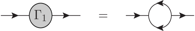
Figure 1: One loop 1PI $2$-point function.

Having discussed the formulation of the superspace action we now outline the strategy taken to carry out the five loop renormalization. One way to gauge the magnitude of a high loop order computation is to tally up the number of Feynman graphs that have to be computed. This has been recorded in Table 1 where the data for the $2$-point function are given. These were compiled using the Qgraf package, [53]. Due to the supersymmetry Ward identity the vertex function is completely finite and so those graphs do not have to be calculated. There are several ways of counting the diagrams for (2.1) which will determine the strategy we will follow. Aside from a superspace approach, where the graph count is given in the final column of Table 1, the theory can be formulated in terms of component fields. For (2.1) one can have real bosonic fields, as in (2.2), or complex ones. The numbers of graphs for the bosonic field $2$-point functions are provided in the table too. Clearly there is a significantly larger number of graphs for both component field calculations. We have chosen not to effect a calculation for either component Lagrangian. This is not merely due to the number of graphs but also because in that case one would have to use dimensional reduction [54] rather than dimensional regularization as the latter does not preserve supersymmetry. The former regularization needs to be implemented with care since additional evanescent fields have to be included in the dimensionally regularized Lagrangian, [55, 56, 57]. By contrast, although the superfield formalism has less than a total of $100$ graphs to compute, the superspace propagator in momentum space for (2.1) is

$$\langle\Phi(p,\theta)\bar{\Phi}(-p,\bar{\theta})\rangle~{}=~{}\frac{\exp{(2\theta p\!\!\!\backslash\bar{\theta}})}{p^{2}}$$ (2.7)

where $p$ is the momentum. Not only is the loop momentum integrated over in superspace Feynman integrals but also the internal $\theta$ coordinates that arise at each vertex of a supergraph. In [4] a different form of the superpropagator was used which involved the supercovariant derivatives $D_{\alpha}$ and $\bar{D}^{\dot{\alpha}}$. These satisfy an algebra, known as the $D$-algebra, which is used to simplify each superspace integral before the integration over the loop momenta can be carried out. Ordinarily the $D$-algebra is implemented by hand, which is straightforward to three loops for (2.1), but this is not a practical approach for higher order calculations. As the superpropagator takes the form (2.7) in (2.1) it is possible to implement the corresponding $D$-algebra in an automatic Feynman diagram calculation. To do so we have written a module in the symbolic manipulation language Form and its threaded version Tform, [58, 59], to achieve this. Indeed the full computation could only be carried out with several key features of the language. For instance, the non-commuting function facility of Form was essential for handling the $D$-algebra. Moreover, once it has been applied to each Feynman graph they can each be evaluated in dimensional regularization which is what we use throughout.

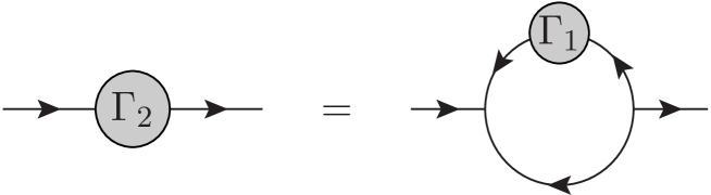
Figure 2: Two loop 1PI $2$-point function.

3 Computational details.

We now discuss the technical aspects behind the five loop calculation which will involve explaining the algorithm for constructing an automatic five loop evaluation. In order to provide the necessary introduction to all the ingredients required for this we focus on the lower loop Feynman graphs for the moment and outline the first step of the process which is to reduce the superspace integrals to momentum space ones. For instance the one and two loop graphs contributing to the $1$-particle irreducible $\Phi$ $2$-point function are illustrated in Figures 1 and 2. Our notation throughout will be that Feynman graphs in superspace will have directed lines as in these two figures. In this respect we note that from (2.1) the arrows on a propagator will all be directed towards the vertex or away. The immediate consequence for this is that there are no Feynman diagrams with subgraphs with an odd number of propagators. This is evident in Figures 1 and 2 as well as ones that appear later. Though where some figures have undirected propagators these represent Feynman integrals in ordinary momentum space and not superspace. We will also use $\Gamma_{n}$ to denote the $1$-particle irreducible graphs at $n$ loops and $C_{n}$ to indicate the connected $2$-point Green’s function at the same order. This will simplify our illustration of the higher loop contributions to the $2$-point function.

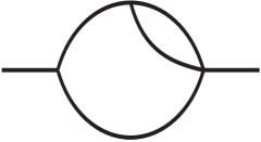
Figure 3: Momentum space representation of $\Gamma_{2}$.

For $\Gamma_{1}$ and $\Gamma_{2}$ the $D$-algebra is simple to implement. Since the $\theta$ and $\bar{\theta}$ dependence in (2.7) is in the exponential of each propagator then each graph will have one exponential that depends on all the anticommuting variables of each vertex of a Feynman diagram. So, for example, since $\Gamma_{1}$ has only two external vertices the overall exponential only depends on the external vertex variables and factors off consistent with renormalizability in superspace. In fact this is a feature of all higher loop graphs where the same factor emerges overall, [6]. Moreover when $\Gamma_{1}$ appears embedded in a higher loop graph this factor that was external contributes to the $D$-algebra calculation of the remaining part of the higher loop graph. So for $\Gamma_{2}$ the only anticommuting variable dependence that remains is a factor $\exp{(2\theta_{1}k\!\!\!\backslash\bar{\theta}_{1}})$ where $k$ is the loop momentum and $\theta_{1}$ and $\bar{\theta}_{1}$ are to be integrated over, [6]. This is after a change of variables on the original internal anticommuting variables. Expanding the exponential then only the quadratic terms are relevant for the $\theta_{1}$ and $\bar{\theta}_{1}$ integration after a trace is taken over the $\sigma^{\mu}$ matrices, [6]. This is readily carried out by mapping the traces to the usual $\gamma$-matrix trace routine but adjusted so that the trace normalization is $2$ and not $4$. The resulting momentum space Feynman integral is represented by the graph of Figure 3. We have detailed this relatively simple calculation as it is an example of a deeper observation for the $D$-algebra of $2$-point subgraphs in higher loop graphs. It turns out that in the resulting momentum space integral one of the propagators connecting any $\Gamma_{n}$ subgraph is deleted in the same way as in Figure 3. This lemma was useful in the five loop calculation.

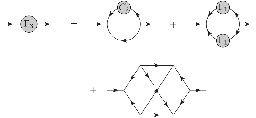
Figure 4: Three loop 1PI $2$-point function.

At next order the $4$ three loop graphs are summarized in Figure 4 where $C_{2}$ contains two diagrams. The non-planar graph is primitive and is divergent. This is in contrast to the identical momentum space non-planar integral with undirected edges which is finite being equal to $20\zeta_{5}$ where $\zeta_{n}$ is the Riemann zeta function. See, for example, the articles [60, 61, 62, 63] for the early discussion on the connection of the Riemann zeta series with the topology of high loop Feynman graph. To evaluate the primitive graph the $D$-algebra needs to be applied. This results in a set of momentum space integrals that are given in Figure 5. In displaying these we note that in total there are $14$ integrals but we have used left-right and up-down symmetry to reduce these to the four independent topologies. The non-planar graph contains the irreducible numerator which becomes apparent when the trace is taken over the fermion propagators which are represented by the dotted lines. It is important to note that these integrals result from the $D$-algebra and have no connection with the Feynman integrals that one would have to compute using the component Lagrangian. We have detailed the reduction for this graph as it differs from the way it was evaluated in the four loop calculation of [6]. There the external momentum was nullified in the numerator of the integral after carrying out the integration over the anticommuting superspace coordinates. For the five loop renormalization we have to determine the integral to the $O(\epsilon)$ term rather than just isolate the divergence. We note that comment was also made in [64] as to how to effect the $D$-algebra for this topology.

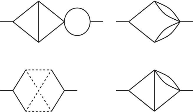
Figure 5: Momentum space integrals after applying the $D$-algebra to the three loop non-planar graph.

At the next loop order the $13$ $2$-point function graphs are given in Figure 6 where we have introduced a shorthand definition of the two loop non-planar vertex which will be denoted by $V_{2}$ and is defined in Figure 7. The subgraph $\bar{V}_{2}$ of Figure 6 corresponds to the graph of Figure 7 but with the direction of the external legs reversed which is the origin of the conjugate notation. In Figure 6 and later figures we do not display all the subgraph mirror images. To illustrate what we mean by subgraph mirror image there is another graph similar to the final graph on the first row of Figure 6 where the $\bar{V}_{2}$ subgraph is translated to the other external vertex whence it would become $V_{2}$. However in performing this translation there is no reflection of the direction of any of the propagators which remains unchanged. The graphs of Figure 6 follow a similar pattern to those at three loops in that the majority are decorations of the previous loop order. This includes the three cases where there are propagator corrections on the three loop primitive. The remaining undecorated planar four loop graph is a primitive at this order. It will have to be evaluated without the re-routing simplification that was used in [6] since we will need the finite part. Moreover it transpires that there are a significantly larger number of momentum space integrals that result from the $D$-algebra compared to those of the three loop primitive.

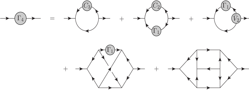
Figure 6: Four loop 1PI $2$-point function.

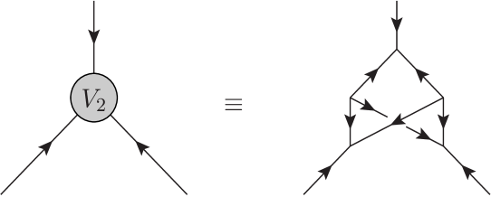
Figure 7: Two loop non-planar vertex correction.

Although our aim is to renormalize (2.1) to five loops we pause at this point to discuss the techniques we used to evaluate the momentum space integrals. To four loops the main tools we employed were the three and four loop packages Mincer, [22, 23], and Forcer, [20, 21], respectively. These are Form encoded packages that evaluate dimensionally regularized $2$-point functions up to various orders in $\epsilon$. While Mincer is tied to theories in four dimensions Forcer has the capacity to determine the $\epsilon$ expansion of momentum space integrals in theories with even critical dimensions. The usefulness of Mincer for example in its application to the Wess-Zumino model is that it can determine the part of the $\beta$-function that solely involves rational numbers to five loops. While it can equally be applied to the evaluation of most of the four loop graphs we had to use Forcer to find the primitive of Figure 6 to the finite part. Another technique we used, that is not limited to the computation of $2$-point functions, was the Laporta algorithm [19] encoded in the Reduze package, [65, 66]. This was primarily required to check the four loop primitive graphs but was also used more extensively at five loops to verify the simple pole of certain difficult primitives. In applying both Mincer and Forcer to all the momentum space integrals that result from the $D$-algebra we have verified the four loop $\beta$-function of [6]. As far as we are aware this is the first direct evaluation of the graphs where there has been simplification involving the external momenta to extract the divergences.

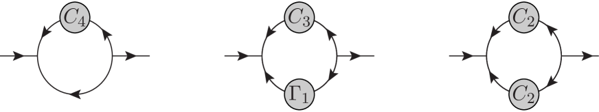
Figure 8: Five loop graphs based on the decoration of $\Gamma_{1}$.

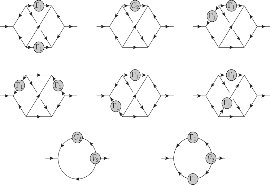
Figure 9: Five loop graphs based on decoration of three loop primitive graph.

4 Five loop calculation.

We turn now to the details of the five loop renormalization which first requires the evaluation of the $63$ graphs. We have chosen to illustrate these in a sequence of Figures and classify the graphs by the underlying skeleton topology. Those given by propagator dressings of $\Gamma_{1}$ are shown in Figure 8 where we note that $C_{3}$ and $C_{4}$ include the respective three and four loop primitives. As all the subgraphs within $C_{n}$ and $\Gamma_{n}$ in the figure are available to the finite part from lower loop computations their contributions to $\gamma_{\Phi}(a)$ are straightforward to determine. However this is not the case for the decoration of the three loop primitive where the graphs are illustrated in Figure 4. The reason for this is that after performing the superspace integration over the internal anticommuting coordinates the set of momentum space integrals do not have a direct correspondence with the decoration of the topologies of Figure 5 in all possible ways. This is not unrelated to the irreducible scalar products that arise. For an $L$ loop $2$-point Feynman graph there are $\mbox{\small{$\frac{1}{2}$}}(L-1)(L-2)$ irreducible scalar products. So to address this issue using a Laporta algorithm approach would require an integral reduction of significant size. Instead as the four loop Forcer package has no direct applicability we have followed a different tactic and that is to apply the method outlined in the five loop renormalization of QCD in [25]. There the divergent part of similar five loop integrals was determined by a combination of infrared rearrangement and the method of subtractions. The external momentum is re-routed through the graph such that it enters through one current external vertex but exits via the first vertex adjacent to that one. For some of the graphs of Figure 9 there are several ways of achieving this which gives a check on the procedure. As noted in [25] this produces an integral containing a four loop $2$-point subgraph that can then be evaluated using the Forcer algorithm, [20, 21]. In other words this package is used indirectly to extract the five loop divergences. For the Wess-Zumino model there are several additional simplifications compared to the QCD case. Aside from the fact that the superspace graphs are zero dimensional, there are fewer graphs and within these there are a small set of irreducible scalar products. Therefore we have constructed a procedure to effect the subtraction approach for the subset of graphs of Figure 9. As a check on our method we have applied it to the similar decorations of the three loop primitive shown in Figure 6 since we know the correct answer from their direct evaluation in Forcer.

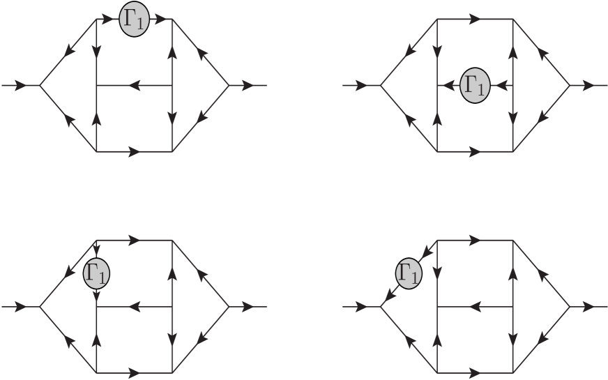
Figure 10: Five loop graphs based on decoration of four loop primitive graph.

In applying that check we thereby verify that it is a valid procedure for evaluating the decoration of the four loop primitive graph of Figure 6. The corresponding representative five loop graphs are shown in Figure 10 and it is clear that the re-routing approach that exploits Forcer is one of the few strategies we have. However for this skeleton topology we were also able to check both poles in $\epsilon$ of the four graphs of Figure 10 by following the algorithm given in [6] for the underlying four loop graph. That method did not re-route the external momentum but set the external momentum to zero where it appeared in the numerator of the integral after the $D$-algebra had been applied. At five loops this produced a topology with a four loop $2$-point subgraph which had a different structure to that of the external momentum re-routing but which could equally well be evaluated using Forcer. For each of the four cases we obtained consistent expressions for the divergences.

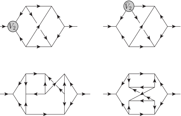
Figure 11: Five loop primitive graphs.

The final subset of graphs for the five loop renormalization are provided in Figure 11 and are the primitives. These can be divided into two classes. One class involves the decoration of the three loop primitives by non-planar vertex corrections. In fact the first graph on the top row is $\Gamma_{1}$ where both external vertices are dressed with $V_{2}$ and $\bar{V}_{2}$. For both these graphs we have evaluated them in several different ways. For the double dressing of $\Gamma_{1}$, for instance, we can merely multiply the pole of $\Gamma_{1}$ by the finite value of $V_{2}$. We have determined this by computing the two loop vertex function using either Mincer or Forcer with one external momentum nullified. As an alternative we have also computed the underlying integral without any restriction on the external momentum. In other words the integral is evaluated at a non-exceptional subtraction point. More specifically we considered the fully symmetric point where the squares of the external momenta are all equal. After applying the Form $D$-algebra module we used the Reduze encoding of the Laporta algorithm to express the diagram in terms of the various two loop master integrals which are available in [67, 68, 69, 70]. Either method produces the value of $3\zeta_{3}$ for the finite part of $V_{2}$ and its conjugate. With this value it transpires that both graphs in the top row of Figure 11 are proportional to $\zeta_{3}^{2}$. In each case we have checked this argument by re-routing the external momentum. As the graphs are primitive where the momentum enters the graph and leaves is not important as long as it is at two separate vertices. This includes the case where only one external momentum is re-routed which we used on the lower loop decorated primitives. The divergence was extracted using Forcer. Whichever approach we used the same simple pole resulted for both these graphs. It also tallies with the method used in [6] for the underlying skeleton topology. What is worth noting about this primitive is that in non-supersymmetric models graphs with a non-planar vertex subgraph correction would not ordinarily be regarded as a primitive. Indeed in the conventional understanding of the appearance of $\zeta_{n}$ to five loops in $2$-point function calculations the primitives are associated with $\zeta_{3}$, $\zeta_{5}$ and $\zeta_{7}$. This product of $\zeta_{n}$ values in a primitive appears to be solely peculiar to the Wess-Zumino model. This leaves the graphs of the lower row of Figure 11 to evaluate. These do not have any vertex subgraphs and so we do not have the same guidance into the final residue of the simple pole. However we have applied the same techniques to extract the divergence and find that both involve the underlying number which is $\frac{441}{8}\zeta_{7}$ if one omits the symmetry factor. That this combination appears is not surprising since it is not unrelated to a parallel primitive Feynman graph in scalar $\phi^{4}$ theory. In [61, 62, 63, 71] the primitive graph was evaluated by the use of conformal integration or the uniqueness method, [72, 73, 74], after an initial numerical evaluation [61, 62, 63]. In fact the residue was also recorded for what is termed the zigzag graph in the prescient work of Broadhurst in [60]. In particular it is recorded in Table 3 of that article where it corresponds to diagram c of Figure 6 there. The residue of the other five loop primitive shown in the first row of Figure 11 is also apparent in Table 3 of [60] via diagrams d and e of Figure 6. The fact that the zigzag topology arises in the seemingly topologically unconnected lower row graphs of Figure 11 is as a consequence of the $D$-algebra. In the simplification of the numerator scalar products after using the method of [6] several propagators are deleted to leave the zigzag graph.

Having outlined in detail in this and the previous section how we have evaluated all the diagrams to five loops to the requisite order in $\epsilon$ to carry out the full renormalization we now note some of the practical aspects of the automatic routine we have constructed. First all the superspace graphs are generated electronically using the Fortran based Qgraf package, [53]. To ease the implementation of the $D$-algebra routine that we have written we use the Qgraf setting that equates to the Mincer or Forcer setup where each propagator is allocated a momentum $p_{i}$. After the $D$-algebra has been carried out either the energy-momentum conservation is implemented at each vertex to reduce the number of $p_{i}$ to the number of loops or values of each $p_{i}$ are substituted explicitly. The latter is used for the cases where the Reduze package was required since the integral families are defined by the explicit values of the internal loop momenta. This represents the core of the integration routine. Though for those five loop graphs where a re-routing was necessary to find the divergence the value was constructed in a separate routine and the result included in the automatic calculation which reduces the run time. This is particularly important since although the focus thus far has been on the renormalization of (2.1) we have also considered extensions of this action such as that with $O(N)$ symmetry which have a significantly larger number of graphs to be determined. Once all the graphs have been computed they are summed before the renormalization is carried out. This follows the established routine of [75] where the calculation is carried out for bare parameters which in the Wess-Zumino case is the coupling constant. Its renormalized partner is introduced through (2.3). As there is one independent renormalization constant the coupling constant counterterms are formally deduced by iteratively solving (2.4) and expressing them in terms of the $Z_{\Phi}$ counterterms. These relations are then included in the routine that ultimately determines the values of the $Z_{\Phi}$ counterterms. We close with a final remark on the evaluation of the diagrams. Although early loop computations of the $\beta$-function primarily concentrated on extracting the result in the $\overline{\mbox{MS}}$ scheme, in [4] the $\beta$-function in the momentum (MOM) subtraction scheme was also determined at three loops. This required knowledge of the higher order terms in the $\epsilon$ expansion of each Feynman graph to two loops. Those at three loop were not necessary, [4], as they would contribute to the four loop MOM $\beta$-function. Therefore, as we have used Forcer to compute the four loop graphs we have also found the finite part of those diagrams as well as the $O(\epsilon)$ terms. So we will also be able to determine the five loop MOM scheme $\beta$-function for (2.1) and its extensions.

5 Results.

After discussing the technical details of how we evaluated all $63$ five loop graphs we now provide the results together with comments on internal checks on the final renormalization group functions. We find in the $\overline{\mbox{MS}}$ scheme that the field anomalous dimension is

$$\gamma_{\Phi}(a) = \frac{1}{2}a~{}-~{}\frac{1}{2}a^{2}~{}+~{}\left[12\zeta_{3}+5\right]\frac{a^{3}}{8}~{}+~{}\left[18\zeta_{4}-60\zeta_{3}-80\zeta_{5}-9\right]\frac{a^{4}}{8}$$ (5.1)

$$+~{}\left[504\zeta_{3}^{2}+858\zeta_{3}-441\zeta_{4}+1828\zeta_{5}-900\zeta_{6}+2646\zeta_{7}+79\right]\frac{a^{5}}{32}~{}+~{}O(a^{7})$$

implying

$$\beta(a) = \frac{3}{2}a^{2}~{}-~{}\frac{3}{2}a^{3}~{}+~{}\left[36\zeta_{3}+15\right]\frac{a^{4}}{8}~{}+~{}\left[54\zeta_{4}-180\zeta_{3}-240\zeta_{5}-27\right]\frac{a^{5}}{8}$$ (5.2)

$$+~{}\left[1512\zeta_{3}^{2}+2574\zeta_{3}-1323\zeta_{4}+5484\zeta_{5}-2700\zeta_{6}+7938\zeta_{7}+237\right]\frac{a^{6}}{32}$$

$$+~{}O(a^{7})$$

for the $\beta$-function which are some of the main results of the article. In arriving at (5.1) the non-simple poles of $Z_{\Phi}$ are not independent from the property of the renormalization group and are related to the residues of the lower loop order poles. That this is consistent validates that aspect of the calculation. Another non-trivial check on the result will be discussed in a later section. Also structurally the five loop $\beta$-function is formally the same as its scalar $\phi^{4}$ counterpart, [61, 62, 63, 75], in terms of the rational and irrational dependence.

As the MOM scheme was considered in [4] we can also provide the renormalization group functions to five loops for that case. For (2.1) the MOM scheme is defined such that at the subtraction point there are no $O(a)$ corrections to the $2$-point function. In other words after renormalization in that scheme the $2$-point function is unity in superspace at the subtraction point. This will determine the MOM expression for $Z_{\Phi}$. However in extracting it from the $2$-point function the coupling constant has also to be renormalized in the same scheme. This is effected by ensuring that the supersymmetry Ward identity (2.4) is preserved as otherwise the scheme would not be consistent with this symmetry. Applying this procedure to the $2$-point function and retaining the necessary terms depending on $\epsilon$ at each loop order we arrive at the results

$$\gamma_{\Phi}^{\mbox{\footnotesize{MOM}}}(a) = \frac{1}{2}a~{}-~{}\frac{1}{2}a^{2}~{}+~{}\left[6\zeta_{3}+7\right]\frac{a^{3}}{4}~{}-~{}\left[13\zeta_{3}+20\zeta_{5}+20\right]\frac{a^{4}}{2}$$ (5.3)

$$+~{}\left[216\zeta_{3}^{2}+772\zeta_{3}+230\zeta_{5}+1323\zeta_{7}+1222\right]\frac{a^{5}}{16}~{}+~{}O(a^{6})$$

and

$$\beta^{\mbox{\footnotesize{MOM}}}(a) = \frac{3}{2}a^{2}~{}-~{}\frac{3}{2}a^{3}~{}+~{}3\left[6\zeta_{3}+7\right]\frac{a^{4}}{4}~{}-~{}3\left[13\zeta_{3}+20\zeta_{5}+20\right]\frac{a^{5}}{2}$$ (5.4)

$$+~{}3\left[216\zeta_{3}^{2}+772\zeta_{3}+230\zeta_{5}+1323\zeta_{7}+1222\right]\frac{a^{6}}{16}~{}+~{}O(a^{7})$$

where both are provided for later purposes. Our convention is that when a renormalization group function is labelled with MOM then the coupling constant $a$ is the MOM coupling constant rather than the $\overline{\mbox{MS}}$ one. For cases where there is potential ambiguity we denote the MOM coupling constant by $a^{\mbox{\footnotesize{MOM}}}$. Where this no ambiguity $a$ will be regarded as the $\overline{\mbox{MS}}$ variable. There are several interesting features of (5.3) and (5.4). First the coefficients of the one and two loop terms of $\gamma_{\Phi}^{\mbox{\footnotesize{MOM}}}(a)$ are the same as the $\overline{\mbox{MS}}$ $\gamma_{\Phi}(a)$. This is a consequence of the supersymmetry Ward identity ensuring the $\beta$-function and $\gamma_{\Phi}(a)$ are proportional. It appears to contradict the accepted position that only the $\beta$-function in a single coupling theory is scheme independent at two loops. In scalar $\phi^{4}$ theory the two loop term of the field anomalous dimension is independent of the renormalization scheme but this is for a trivial reason since it is the first non-zero term. The other peculiar feature of (5.3) for example is that there are no terms involving $\zeta_{2n}$. In other words only the odd integer argument Riemann zeta function numbers are present. Hence there are no terms which involve even powers of $\pi$ at least to five loops.

While we have found the five loop result for $\gamma_{\Phi}^{\mbox{\footnotesize{MOM}}}(a)$ by direct evaluation it is possible to determine it by another method. This was discussed in [4] and involves constructing the map between the coupling constant in one scheme with that in the other. It only requires the four loop calculation of $Z_{\Phi}$ is each scheme to achieve this. First, we define the two conversion functions

$$C_{g}(a)~{}=~{}\left(\frac{Z_{g}^{\overline{\mbox{\footnotesize{MS}}}}}{Z_{g}^{\mbox{\footnotesize{MOM}}}}\right)^{2}~{}~{}~{}~{},~{}~{}~{}~{}C_{\Phi}(a)~{}=~{}\frac{Z_{\Phi}^{\mbox{\footnotesize{MOM}}}}{Z_{\Phi}^{\overline{\mbox{\footnotesize{MS}}}}}$$ (5.5)

where each renormalization constant depends on the coupling constant in the indicated scheme. Although each renormalization constant has poles in $\epsilon$ the conversion function is finite as $\epsilon$ $\to$ $0$. This is because the variables $a$ and $a^{\mbox{$\mbox{\footnotesize{MOM}}$}}$ are not independent and in fact ensuring $C_{g}(a)$ is finite order by order determines the relation between the two. Thus we find

$$a^{\mbox{\footnotesize{MOM}}} = a\left[1~{}-~{}3a~{}+~{}\frac{57}{4}a^{2}~{}-~{}[64\zeta_{3}+18\zeta_{4}+659]\frac{a^{3}}{8}\right.$$ (5.6)

$$\left.~{}~{}~{}+~{}[2094\zeta_{3}-24\zeta_{3}^{2}+351\zeta_{4}+504\zeta_{5}+300\zeta_{6}+8895]\frac{a^{4}}{16}\right]~{}+~{}O(a^{6})$$

where $a$ on the right side is in the $\overline{\mbox{MS}}$ scheme. Equally once (5.6) has been established the wave function scheme conversion function $C_{\Phi}(a)$ can be deduced as

$$C_{\Phi}(a) = 1~{}-~{}a~{}+~{}\frac{15}{4}a^{2}~{}-~{}[64\zeta_{3}+18\zeta_{4}+471]\frac{a^{3}}{24}$$ (5.7)

$$+~{}[1838\zeta_{3}-24\zeta_{3}^{2}+279\zeta_{4}+504\zeta_{5}+300\zeta_{6}+6156]\frac{a^{4}}{48}~{}+~{}O(a^{5})~{}.$$

Equipped with these relations and using the renormalization group formalism the MOM renormalization group functions can be calculated using

$$\beta^{\mbox{$\mbox{\footnotesize{MOM}}$}}(a^{\mbox{$\mbox{\footnotesize{MOM}}$}})~{}=~{}\left[\beta(a)\frac{\partial a_{\mbox{$\mbox{\footnotesize{MOM}}$}}}{\partial a}\right]_{\overline{\mbox{\footnotesize{MS}}}\rightarrow\mbox{\footnotesize{MOM}}}$$ (5.8)

and

$$\gamma_{\Phi}^{\mbox{\footnotesize{MOM}}}(a^{\mbox{\footnotesize{MOM}}})~{}=~{}\left[\gamma_{\Phi}^{\overline{\mbox{\footnotesize{MS}}}}(a)~{}+~{}\beta^{\overline{\mbox{\footnotesize{MS}}}}(a)\frac{\partial~{}}{\partial a}\ln C_{\Phi}^{\mbox{\footnotesize{MOM}}}(a)\right]_{\overline{\mbox{\footnotesize{MS}}}\rightarrow\mbox{\footnotesize{MOM}}}$$ (5.9)

where the restriction indicates that because the quantity inside the square brackets is a function of $a$ it has to be mapped to the $a^{\mbox{$\mbox{\footnotesize{MOM}}$}}$ variable. This is achieved by the mapping which is the inverse of (5.6). Following this we reproduce the five loop MOM results (5.3) and (5.4). Only four loop information is required for this exercise which is also the reason why the finite parts of the five loop Feynman graphs are not required to determine the five loop MOM renormalization group functions.

6 Group valued Wess-Zumino model.

We now turn to a variation on (2.1) which is to have a multiplet of $N$ superfields where the interaction contains a real tensor denoted by $d^{ijk}$ where $1$ $\leq$ $i$ $\leq$ $N$. The bare action is

$$S~{}=~{}\int d^{4}x\!\left[\int d^{2}\theta d^{2}\bar{\theta}\,\bar{\Phi}_{0}^{i}(x,\bar{\theta})e^{-2\theta{\partial\!\!\!\backslash}\bar{\theta}}\Phi_{0}^{i}(x,\theta)\,+\,g_{0}\frac{d^{ijk}}{3!}\!\int d^{2}\theta\,\Phi_{0}^{i}\Phi_{0}^{j}\Phi_{0}^{k}\,+\,g_{0}\frac{d^{ijk}}{3!}\!\int d^{2}\bar{\theta}\,\bar{\Phi}_{0}^{i}\bar{\Phi}_{0}^{j}\bar{\Phi}_{0}^{k}\right]$$ (6.1)

where the aim is to determine the coupling constant renormalization. The notation for the tensor derives from that of six dimensional scalar $\phi^{3}$ theory [77, 78]. To accommodate the different combinations of tensors that appear in loop calculations a useful notation was also provuided in [77, 78] and extended to the four loop renormalization in [79]. This will introduce scalar objects $T_{i}$ that play a similar role as the group Casimirs of a non-abelian gauge theory. As the diagrams comprising the $2$-point function of (6.1) only have subgraphs with an even number of propagators, we only need to recall the relevant tensor combinations that will appear to five loops. These are

$$T_{2}\delta^{ij}~{}=~{}d^{ii_{1}i_{2}}d^{ji_{1}i_{2}}$$

$$T_{5}d^{ijk}~{}=~{}d^{ii_{1}i_{2}}d^{ji_{3}i_{4}}d^{ki_{5}i_{6}}d^{i_{1}i_{3}i_{5}}d^{i_{2}i_{4}i_{6}}$$

$$T_{71}d^{ijk}~{}=~{}d^{ii_{1}i_{2}}d^{ji_{3}i_{4}}d^{ki_{5}i_{6}}d^{i_{1}i_{3}i_{7}}d^{i_{2}i_{5}i_{8}}d^{i_{4}i_{6}i_{9}}d^{i_{7}i_{8}i_{9}}$$

$$T_{94}d^{ijk}~{}=~{}d^{ii_{1}i_{2}}d^{ji_{3}i_{4}}d^{ki_{5}i_{12}}d^{i_{1}i_{5}i_{6}}d^{i_{2}i_{7}i_{8}}d^{i_{3}i_{9}i_{12}}d^{i_{4}i_{10}i_{11}}d^{i_{6}i_{7}i_{10}}d^{i_{8}i_{9}i_{11}}~{}.$$ (6.2)

The first digit of the subscript of any $T_{i}$ indicates the number of $d^{ijk}$ tensors comprising the underlying graph or equivalently the number of propagators. So $T_{2}$ denotes the one loop $2$-point bubble. The others correspond to vertex functions at two, three and four loops respectively. Contracting these tensors with another tensor produces a $2$-point function topology. These then isolate the respective three and four loop primitive graphs of Figures 4 and 6. At five loops the graphs that involve $T_{94}$ are those of the lower row of Figure 11. Those in the top row involve $T_{5}^{2}$. One advantage of this notation is that the contribution to the renormalization group functions from the primitive at each loop order can be identified and followed within a calculation. Such an analysis was performed for scalar $\phi^{4}$ theory in [34] and suggested that the percentage contribution from the primitive graphs at each loop order increases with the number of loops.

Therefore we have computed the renormalization group functions for (6.1) and find

$$\gamma_{T}(a) = \frac{1}{2}T_{2}a~{}-~{}\frac{1}{2}T_{2}^{2}a^{2}~{}+~{}T_{2}\left[12\zeta_{3}T_{5}+5T_{2}^{2}\right]\frac{a^{3}}{8}$$ (6.3)

$$+~{}T_{2}\left[18\zeta_{4}T_{2}T_{5}-60\zeta_{3}T_{2}T_{5}-80\zeta_{5}T_{71}-9T_{2}^{3}\right]\frac{a^{4}}{8}$$

$$+~{}T_{2}\left[12\zeta_{3}T_{2}^{4}+79T_{2}^{4}+846\zeta_{3}T_{2}^{2}T_{5}-441\zeta_{4}T_{2}^{2}T_{5}-612\zeta_{5}T_{2}^{2}T_{5}-216\zeta_{3}^{2}T_{2}T_{71}\right.$$

$$\left.~{}~{}~{}~{}~{}~{}~{}+2440\zeta_{5}T_{2}T_{71}-900\zeta_{6}T_{2}T_{71}+720\zeta_{3}^{2}T_{5}^{2}+2646\zeta_{7}T_{94}\right]\frac{a^{6}}{32}~{}+~{}O(a^{7})$$

for the anomalous dimension in the $\overline{\mbox{MS}}$ scheme. As there is only one coupling and chiral field in (6.1) the original supersymmetry Ward identity (2.4) is satisfied. At the same time it is a simple matter to determine the MOM scheme version of (6.3) giving

$$\gamma_{T}^{\mbox{\footnotesize{MOM}}}(a) = \frac{1}{2}T_{2}a~{}-~{}\frac{1}{2}T_{2}^{2}a^{2}$$ (6.4)

$$+~{}T_{2}\left[6\zeta_{3}T_{5}+7T_{2}^{2}\right]\frac{a^{3}}{4}~{}-~{}T_{2}\left[15\zeta_{3}T_{2}T_{5}-2\zeta_{3}T_{2}^{3}+20\zeta_{5}T_{71}+20T_{2}^{3}\right]\frac{a^{4}}{2}$$

$$+~{}T_{2}\left[1222T_{2}^{4}-164\zeta_{3}T_{2}^{4}+936\zeta_{3}T_{2}^{2}T_{5}-810\zeta_{5}T_{2}^{2}T_{5}-144\zeta_{3}^{2}T_{2}T_{71}\right.$$

$$\left.~{}~{}~{}~{}~{}~{}~{}~{}+1040\zeta_{5}T_{2}T_{71}+360\zeta_{3}^{2}T_{5}^{2}+1323\zeta_{7}T_{94}\right]\frac{a^{5}}{16}~{}+~{}O(a^{6})$$

where like (5.4) there are no even zetas. Formally setting $T_{i}$ $=$ $1$ for all $i$ recovers the analogous equations of the previous section. It is clear from both expressions that the coefficients of the primitives are unchanged at the loop order where they first appear. We note that the coupling constant map is

$$a_{T}^{\mbox{\footnotesize{MOM}}} = \left[1~{}-~{}3T_{2}a~{}+~{}\frac{57}{4}T_{2}^{2}a^{2}~{}-~{}T_{2}[72\zeta_{3}T_{2}^{2}-8\zeta_{3}T_{2}T_{5}+18\zeta_{4}T_{2}T_{5}+659T_{2}^{2}]\frac{a^{3}}{8}\right.$$ (6.5)

$$\left.~{}+T_{2}[8895T_{2}^{3}-300\zeta_{3}T_{2}^{3}+2394\zeta_{3}T_{2}T_{5}+351\zeta_{4}T_{2}T_{5}-336\zeta_{5}T_{2}T_{5}-24\zeta_{3}^{2}T_{71}\right.$$

$$\left.~{}~{}~{}~{}~{}~{}~{}~{}+840\zeta_{5}T_{71}+300\zeta_{6}T_{71}]\frac{a^{4}}{16}\right]a~{}+~{}O(a^{6})~{}.$$

To gauge the primitive contribution the numerical evaluations of (6.3) and (6.4) are

$$\gamma_{T}(a) = \frac{1}{2}T_{2}a-\frac{1}{2}T_{2}^{2}a^{2}+T_{2}\left[0.625T_{2}^{2}+1.803085T_{5}\right]a^{3}$$ (6.6)

$$-~{}T_{2}\left[1.125T_{2}^{3}+6.580199T_{2}T_{5}+10.369277T_{71}\right]a^{4}$$

$$+~{}T_{2}\left[2.919521T_{2}^{4}-2.967631T_{2}^{2}T_{5}+38.872050T_{2}T_{71}+32.511168T_{5}^{2}\right.$$

$$\left.~{}~{}~{}~{}~{}~{}~{}+83.377881T_{94}\right]a^{5}~{}+~{}O(a^{6})$$

and

$$\gamma_{T}^{\mbox{\footnotesize{MOM}}}(a) = \frac{1}{2}T_{2}a-\frac{1}{2}T_{2}^{2}a^{2}~{}+~{}T_{2}\left[1.75T_{2}^{2}+1.803085T_{5}\right]a^{3}$$ (6.7)

$$-~{}T_{2}\left[8.797943T_{2}^{3}+9.015427T_{2}T_{5}+10.369277T_{71}\right]a^{4}$$

$$+~{}T_{2}\left[64.053917T_{2}^{4}+17.825861T_{2}^{2}T_{5}+54.395837T_{2}T_{71}+32.511168T_{5}^{2}\right.$$

$$\left.~{}~{}~{}~{}~{}~{}~{}+83.377881T_{94}\right]a^{5}~{}+~{}O(a^{6})$$

respectively. If we recall that at five loops the graphs of the upper row of Figure 11 are what we termed product primitives we can identity their contributions from the coefficient of $T_{2}T_{5}^{2}$. This is because $T_{5}$ is associated with the graph $V_{2}$. If we compute the contribution from the primitives at three, four and five loop order we find that respectively they contribute $74.26\%$, $57.37\%$ and $74.91\%$. At lower orders it is not meaningful to quote values as it would be $100\%$ at one loop and there are no two loop primitives. For the MOM scheme the analogous numbers are $50.75\%$, $36.79\%$ and $45.96\%$. The smaller relative contribution for the MOM scheme is due primarily to the increase in the coefficient of the $T_{2}^{L}$ terms at each loop order $L$. However for the $\overline{\mbox{MS}}$ scheme the observation of [34] that the primitives make an increasing contribution at higher orders for $\phi^{4}$ theory seems to hold here too for the $\overline{\mbox{MS}}$ scheme albeit at one loop order fewer than [34]. It would be interesting if another scheme could be studied for the non-supersymmetric theory.

An additional motivation for examining the $\beta$-function of (6.1) is that it provides another relatively trivial check on our five loop computation. It transpires that the coefficients of the terms of $T_{2}^{L}$ in (6.4) have already been computed before. More specifically we mean the three loop and higher coefficients since the one and two loop terms are scheme independent. We stress that we are indeed referring to the MOM result rather than the $\overline{\mbox{MS}}$ one. In [64, 80, 81] $\gamma_{\Phi}(a)$ was studied using the Hopf algebra construction of Broadhurst and Kreimer, [82, 83]. Specifically it was used to determine the scalar field anomalous dimension in scalar $\phi^{3}$ and scalar Yukawa theories for a specific class of Feynman diagrams. In particular the Dyson-Schwinger equation for embedding of basic one loop propagator correction within the skeleton one loop graph itself was constructed and solved for the anomalous dimension. This was extended in [81] to the Wess-Zumino model where the supersymmetry Ward identity was important in constructing and solving the corresponding Dyson-Schwinger equation. Moreover, it is the first case we believe where the $\beta$-function of any theory was accessed this way in the Hopf approach. Consequently the first $200$ coefficients of $\gamma_{\Phi}(a)$ were determined for (2.1) with the analytic form given for the first $12$ terms for the class of diagrams considered. While the analysis of [81] centred on the theory with action (2.1) a subset of the graphs making up the coefficients of (5.1) were found. These are straightforward to isolate with the labelling used for (6.1). As [81] used the iteration of the one loop bubble the $T_{2}^{L}$ terms of our five loop $\beta$-function should tally with the Hopf algebra case. The question of which scheme was used can be established by the renormalization condition used in [81] and it is clear it corresponds to the MOM one of [4]. This therefore represents a specific check on the $T_{2}^{L}$ coefficients of (6.4).

Having established the five loop renormalization group functions we can now extract estimates for several critical exponents in the $\epsilon$ expansion at the Wilson-Fisher fixed point where again we take $d$ $=$ $4$ $-$ $2\epsilon$. The specific exponents we will compute are $\eta$ $=$ $\gamma_{\Phi}(a^{\ast})$ and the correction to scaling exponent $2\beta^{\prime}(a^{\ast})$ where $a^{\ast}$ is the critical coupling constant. We will denote this combination here and later by $\hat{\omega}$ rather than the more usual unhatted version to avoid conflict with notation in a later section. From (5.2) we find

$$\hat{\omega} = 2\epsilon~{}-~{}\frac{4}{3}\epsilon^{2}~{}+~{}\frac{4}{9}[12\zeta_{3}+1]\epsilon^{3}~{}+~{}\frac{4}{27}[54\zeta_{4}-84\zeta_{3}-240\zeta_{5}-7]\epsilon^{4}$$ (6.8)

$$+~{}\frac{4}{81}[576\zeta_{3}^{2}+396\zeta_{3}-378\zeta_{4}+1416\zeta_{5}-1800\zeta_{6}+5292\zeta_{7}+19]\epsilon^{5}~{}+~{}O(\epsilon^{6})$$

or

$$\hat{\omega} = 2\epsilon~{}-~{}1.333333\epsilon^{2}~{}+~{}6.855415\epsilon^{3}~{}-~{}44.205924\epsilon^{4}~{}+~{}290.935250\epsilon^{5}~{}+~{}O(\epsilon^{6})$$ (6.9)

numerically. The situation with $\eta$ is somewhat simpler in perturbation theory due to the supersymmetry Ward identity as has been noted in [15, 35] for example. As the dimensionality of the coupling constant manifests itself in the $O(a)$ term of $\beta(a)$ in $d$-dimensions then (5.1) implies

$$\eta~{}=~{}\frac{1}{3}\epsilon$$ (6.10)

exactly. For the more general group valued case (6.1), and for later purposes, we note that the critical coupling is

$$a_{T}^{\ast} = \frac{2}{3T_{2}}\epsilon+\frac{4}{9T_{2}}\epsilon^{2}+2[T_{2}^{2}-4\zeta_{3}T_{5}]\frac{\epsilon^{3}}{9T_{2}^{3}}+8[2T_{2}^{3}-9\zeta_{4}T_{2}T_{5}+40\zeta_{5}T_{71}]\frac{\epsilon^{4}}{81T_{2}^{4}}$$ (6.11)

$$+~{}2[16T_{2}^{4}-12\zeta_{3}T_{2}^{4}-54\zeta_{3}T_{2}^{2}T_{5}+9\zeta_{4}T_{2}^{2}T_{5}+612\zeta_{5}T_{2}^{2}T_{5}+216\zeta_{3}^{2}T_{2}T_{71}$$

$$~{}~{}~{}~{}~{}-520\zeta_{5}T_{2}T_{71}+900\zeta_{6}T_{2}T_{71}-288\zeta_{3}^{2}T_{5}^{2}-2646\zeta_{7}T_{94}]\frac{\epsilon^{5}}{243T_{2}^{5}}~{}+~{}O(\epsilon^{6})$$

implying

$$\hat{\omega}_{T} = 2\epsilon~{}-~{}\frac{4}{3}\epsilon^{2}~{}+~{}\frac{4}{9}\epsilon^{3}~{}-~{}\frac{28}{27}\epsilon^{4}~{}+~{}4[24\zeta_{3}+19]\frac{\epsilon^{5}}{81}$$ (6.12)

$$+~{}\left[\frac{16}{3}\zeta_{3}\epsilon^{3}~{}+~{}\frac{8}{9}[9\zeta_{4}-14\zeta_{3}]\epsilon^{4}~{}+~{}\frac{8}{27}[62\zeta_{3}-63\zeta_{4}-204\zeta_{5}]\epsilon^{5}\right]\frac{T_{5}}{T_{2}^{2}}$$

$$+~{}\left[-~{}\frac{320}{9}\zeta_{5}\epsilon^{4}~{}+~{}\frac{32}{27}[110\zeta_{5}-18\zeta_{3}^{2}-75\zeta_{6}]\epsilon^{5}\right]\frac{T_{71}}{T_{2}^{3}}$$

$$+~{}\frac{448}{9}\zeta_{3}^{2}\frac{T_{5}^{2}}{T_{2}^{4}}\epsilon^{5}~{}+~{}\frac{784}{3}\zeta_{7}\frac{T_{94}}{T_{2}^{4}}\epsilon^{5}~{}+~{}O(\epsilon^{6})$$

where we have ordered the expansion in terms of the group invariants. The power of the leading term in $\epsilon$ of each of the invariants tallies with the loop order of the $\beta$-function where the corresponding $T_{i}$ first appears. The leading order $T_{i}$ independent terms correspond to the bubble insertions associated with $T_{2}$ with the primitive ranked by powers of $1/T_{2}$.

$L$	Padé	Value	Average
$2$	$[2,0]$	$0.666667$	$0.666667$
$3$	$[2,1]$	$0.906650$	$0.906650$
$4$	$[3,1]$	$0.869530$
	$[2,2]$	$0.872352$	$0.870940$
$5$	$[4,1]$	$0.879670$
	$[3,2]$	$0.877593$
	$[2,3]$	$0.878492$	$0.878585$

Table 2: Estimates for $\hat{\omega}$ in three dimensions from Padé approximants.

One reason for determining $\hat{\omega}$ in (6.8) is that there has been interest in estimating this exponent in three dimensions using various methods, [15, 18, 35, 36, 37, 38, 39, 84]. Therefore with the five loop extension of (5.2) we can update the four loop $\epsilon$ expansion estimate noted in [38]. To do this we have evaluated Padé approximants which are recorded in Table 2. In addition to the five loop estimates for completeness we have provided lower loop approximants. In the table only estimates in three dimensions are given where there were no singularities in the Padé approximant between $4$ and $3$ dimensions. In other words the approximant has to be continuously connected to the value in the critical dimension. The final column gives the average of the approximants at each loop order. If one focuses on the three and higher loop averages it would appear that the approximants are converging but perhaps oscillating about the true value. In order to place the five loop estimate in perspective we have gathered results from earlier work on the exponent and recorded them chronologically in Table 3. Aside from the $\epsilon$ expansion the two main techniques are the conformal bootstrap and the functional renormalization group. Some comments are in order. Errors on estimates are those given in the corresponding paper. In [37] two sets of values were provided and distinguished by the parameter $n$. We have noted both sets but mention that the authors regarded the $n$ $=$ $2$ data as superior. Also the value we quote for $\hat{\omega}$ is that designated as supersymmetric in Table I of [37]. The bracketed value for $1/\nu$ from [36] was derived from the estimate of $\eta$ using the superscaling law of [37, 85, 86]

$$\frac{1}{\nu}~{}=~{}\frac{1}{2}\left(d~{}-~{}\eta\right)~{}.$$ (6.13)

We have also used this to extract the value recorded in the table from the exact value of $\frac{1}{6}$ for $\eta$ which would imply that $\frac{1}{\nu}$ $=$ $\frac{17}{12}$. In [35] the value of $\nu$ was determined but we have converted it to $\frac{1}{\nu}$ for consistency with the other entries in the table. This was used to deduce $\eta$ from the superscaling law. While the values of the exponents from [84] are noted as $\epsilon$ expansion they are not deduced in the same way as those of this paper. Instead they represent the result of a matched Padé approach where the $\epsilon$ expansion of two theories in the same universality class are used but one theory has a critical dimension of $2$ while the other is renormalizable in $4$. Moreover the universality class is the Gross-Neveu-Yukawa one and the values in the table correspond to those for the emergent supersymmetry. As we took a direct supersymmetric approach our values for $\eta$ and $\frac{1}{\nu}$ are exact due to the supersymmetry Ward identity and are within the errors given in [84]. As an aside we note that the other $\epsilon$ expansion result of [15] did not benefit from a two-sided Padé approach which may be the reason why that estimate for $\frac{1}{\nu}$ is low compared to [84]. In terms of the overall picture there appears to be a consensus that the value of $\eta$ is around $0.166$ especially in the more recent articles that did not have the use of the supersymmetry Ward identity present in the $\epsilon$ expansion. The latest conformal bootstrap value appears to be the most accurate numerically given the precision and tight error bars on $\eta$ and $\frac{1}{\nu}$. Indeed our exact values differ by around $1.3\%$ and $0.08\%$ respectively with both conformal bootstrap values satisfying (6.13). For $\hat{\omega}$ the difference is roughly $0.5\%$.

Method	Reference	$\eta$	$\frac{1}{\nu}_{\frac{}{}}$	$\hat{\omega}$
CB	[18]	$0.166667$	$1.0902(20)$	$0.9098(20)$
FRG	[35]	$0.114$	$1.443$	$0.796$
CB	[36]	$0.164$	$(1.418)$	————–
FRG	[37] $(n=1)$	$0.174$	$1.385$	$0.765$
FRG	[37] $(n=2)$	$0.167$	$1.395$	$0.782$
$\epsilon$	[15]	$0.166667$	$1.129(1)$	$0.871(1)$
FRG	[38]	————–	$1.1656$	$0.8344$
$\epsilon$	[84]	$0.1673(50)$	$1.415(12)$	————–
CB	[39]	$0.168888(60)$	$1.415556(30)$	$0.882(9)$
$\epsilon$	This work	$0.166667$	$1.416667$	$0.878585$

Table 3: Summary of exponent estimates by conformal bootstrap (CB), functional renormalization group (FRG) and $\epsilon$ expansion methods.

One interesting application of considering (6.1) is that the renormalization group functions can be deduced for Lie groups which have a non-trivial rank $3$ fully symmetric tensor $d^{ijk}$. One such class of groups are the $SU(N_{\!c})$ ones and in that case (6.2) reduce to

$$T_{2} = \frac{[N_{\!c}^{2}-4]}{N_{\!c}}~{}~{},~{}~{}T_{5}~{}=~{}-~{}\frac{4}{N_{\!c}^{2}}[N_{\!c}^{2}-10]$$

$$T_{71} = \frac{1}{8N_{\!c}^{3}}[N_{\!c}^{2}-8][N_{\!c}^{4}-8N_{\!c}^{2}+256]$$

$$T_{94} = -~{}[N_{\!c}^{6}-64N_{\!c}^{4}+1216N_{\!c}^{2}-6784]\frac{1}{4N_{\!c}^{4}}$$ (6.14)

using [87]. So, for example, for $SU(3)$ we have

$$\left.\gamma_{\Phi}(a)\right|_{SU(3)} = \frac{5}{6}a-\frac{25}{18}a^{2}+\frac{5}{216}[48\zeta_{3}+125]a^{3}+\frac{25}{648}[72\zeta_{4}-530\zeta_{5}-225-240\zeta_{3}]a^{4}$$ (6.15)

$$+~{}\frac{25}{15552}[36840\zeta_{3}-9702\zeta_{3}^{2}-17640\zeta_{4}+137170\zeta_{5}-59625\zeta_{6}+78057\zeta_{7}$$

$$~{}~{}~{}~{}~{}~{}~{}~{}~{}~{}~{}~{}+19750]a^{5}~{}+~{}O(a^{6})$$

and

$$\left.\beta(a)\right|_{SU(3)} = \frac{5}{2}a^{2}-\frac{25}{6}a^{3}+\frac{5}{72}[48\zeta_{3}+125]a^{4}+\frac{25}{216}[72\zeta_{4}-530\zeta_{5}-225-240\zeta_{3}]a^{5}$$ (6.16)

$$+~{}\frac{25}{5184}[36840\zeta_{3}-9702\zeta_{3}^{2}-17640\zeta_{4}+137170\zeta_{5}-59625\zeta_{6}+78057\zeta_{7}$$

$$~{}~{}~{}~{}~{}~{}~{}~{}~{}~{}+19750]a^{6}~{}+~{}O(a^{7})$$

which we record for later purposes. As there has also been recent interest in Wess-Zumino models with $F_{4}$ symmetry, [46], we note that the corresponding renormalization group functions and exponents can be extracted from (6.3) and (6.12) with

$$T_{3} = -~{}[N-2]\frac{T_{2}}{2[N+2]}~{}~{},~{}~{}T_{5}~{}=~{}-~{}[N^{2}-10N-16]\frac{T_{2}^{2}}{2[N+2]^{2}}$$

$$T_{71} = [N^{3}-3N^{2}+80N+100]\frac{T_{2}^{3}}{4[N+2]^{3}}$$

$$T_{94} = -~{}[N^{4}-14N^{3}-12N^{2}-616N-672]\frac{T_{2}^{4}}{8[N+2]^{4}}$$ (6.17)

where $N$ is the dimension of an $F_{4}$ representation such as $\mathbf{2}$, $\mathbf{5}$, $\mathbf{8}$, $\mathbf{14}$, $\mathbf{26}$, $\mathbf{27}$, $\mathbf{90}$ or $\mathbf{324}$.

7 $O(N)$ Wess-Zumino model.

As a second generalization of (2.1) we consider the Wess-Zumino model with an $O(N)$ symmetry as it will provide us with another check on our computation. This is because the $O(N)$ model admits a large $N$ expansion and the renormalization group functions have been computed to three orders in powers of $1/N$ in [48, 49]. The action in terms of bare quantities is

$$S^{O(N)} = \int d^{4}x\left[\int d^{2}\theta d^{2}\bar{\theta}\,\bar{\Phi}_{0}^{i}(x,\bar{\theta})e^{-2\theta{\partial\!\!\!\backslash}\bar{\theta}}\Phi_{0}^{i}(x,\theta)~{}+~{}\bar{\sigma}_{0}(x,\bar{\theta})e^{-2\theta{\partial\!\!\!\backslash}\bar{\theta}}\sigma_{0}(x,\theta)\right.$$ (7.1)

$$\left.~{}~{}~{}~{}~{}~{}~{}~{}~{}+~{}\frac{{g_{1}}_{0}}{2}\int d^{2}\theta\,\sigma_{0}\Phi_{0}^{i}\Phi_{0}^{i}~{}+~{}\frac{{g_{1}}_{0}}{2}\int d^{2}\bar{\theta}\,\bar{\sigma}_{0}\bar{\Phi}_{0}^{i}\bar{\Phi}_{0}^{i}\right.$$

$$\left.~{}~{}~{}~{}~{}~{}~{}~{}~{}+~{}\frac{{g_{2}}_{0}}{6}\int d^{2}\theta\,\sigma_{0}^{3}~{}+~{}\frac{{g_{2}}_{0}}{6}\int d^{2}\bar{\theta}\,\bar{\sigma}_{0}^{3}\right]$$

and was given in [88] where $1$ $\leq$ $i$ $\leq$ $N$. We regard the coupling constants as real. In [88] they were taken to be complex but they will only appear as squares in the renormalization group functions. In this case this combination will be equivalent to the squared length of $g_{1}$ and $g_{2}$ respectively given in [88]. The superfields $\Phi^{i}$ and $\bar{\Phi}^{i}$ lie in an $O(N)$ multiplet and the $\sigma$ and $\bar{\sigma}$ fields would equate to auxiliary fields in non-supersymmetric four dimensional $\phi^{4}$ theory. In other words in that instance the quartic interaction can be rewritten as a cubic interaction, akin to that of (7.1) with the $g_{1}$ coupling constant, and a non-kinetic quadratic term equivalent to that for $\sigma$ and $\bar{\sigma}$ but without the $\theta$ dependent exponential. For that reason one can regard the $O(N)$ Wess-Zumino model as a supersymmetric generalization of $O(N)$ scalar $\phi^{4}$ theory. This is apparent in the purely bosonic sector of the component Lagrangian (2.2). Indeed it is that rewriting of the quartic interaction that is the key to accessing the large $N$ expansion through the critical point formalism developed in $d$-dimensions in [73, 74, 89] for scalar $\phi^{4}$ theory as we will show later. This was extended in [48, 49] for (7.1) where more background on this aspect to exploring the Wess-Zumino model can be found. It is also worth noting that when both couplings are non-zero the action is formally equivalent to that of non-supersymmetric $O(N)$ $\phi^{3}$ theory in six dimensions that was analysed at three loops in [79, 90]. This is in the sense that in six dimensions there are two interactions that ensure the theory is renormalizable. Finally we note that the $O(N)$ Wess-Zumino model also has only two independent renormalization constants which can be expressed as

$$\beta_{1}^{O(N)}(g_{i})~{}=~{}\frac{1}{2}g_{1}\left[\gamma^{O(N)}_{\sigma}(g_{i})~{}+~{}2\gamma^{O(N)}_{\Phi}(g_{i})\right]~{}~{},~{}~{}\beta_{2}^{O(N)}(g_{i})~{}=~{}\frac{3}{2}g_{2}\gamma^{O(N)}_{\sigma}(g_{i})$$ (7.2)

where $\gamma_{\sigma}(g_{i})$ is the anomalous dimension of the $\sigma$ and $\bar{\sigma}$ superfields and we use $g_{i}$ as shorthand for pair of couplings $\{g_{1},g_{2}\}$.

$L$	$\Phi$	$\sigma$
$1$	$1$	$2$
$2$	$3$	$3$
$3$	$15$	$20$
$4$	$109$	$124$
$5$	$952$	$1063$
Total	$1080$	$1212$

Table 4: Number of graphs at each loop order $L$ for the $\Phi$ and $\sigma$ superfield $2$-point functions in the $O(N)$ Wess-Zumino model.

To extract the renormalization group functions for (7.1) using Qgraf we have generated all the supergraphs to five loops required for renormalizing the $\Phi^{i}$ and $\sigma$ $2$-point functions. The number of graphs that we had to compute at each loop order are listed in Table 4. With these graphs as input we applied the automatic integration routine that was outlined earlier and extracted the corresponding renormalization group functions which are included in the attached data file. To five loops we found

$$\beta_{1}^{O(N)}(g_{i}) = \left[\frac{1}{2}g_{1}g_{2}^{2}+2g_{1}^{3}+\frac{1}{2}Ng_{1}^{3}\right]+\left[-\frac{1}{2}g_{1}g_{2}^{4}-g_{1}^{3}g_{2}^{2}-2g_{1}^{5}-\frac{1}{2}Ng_{1}^{3}g_{2}^{2}-2Ng_{1}^{5}\right]$$ (7.3)

$$+\left[\frac{5}{8}g_{1}g_{2}^{6}+\frac{3}{2}g_{1}^{3}g_{2}^{4}+g_{1}^{5}g_{2}^{2}+2g_{1}^{7}+\frac{1}{4}Ng_{1}^{3}g_{2}^{4}+4Ng_{1}^{5}g_{2}^{2}+\frac{11}{2}Ng_{1}^{7}-\frac{3}{8}N^{2}g_{1}^{5}g_{2}^{2}\right.$$

$$\left.~{}~{}~{}+\frac{1}{2}N^{2}g_{1}^{7}+\frac{3}{2}\zeta_{3}g_{1}g_{2}^{6}+12\zeta_{3}g_{1}^{5}g_{2}^{2}+12\zeta_{3}g_{1}^{7}+\frac{15}{2}\zeta_{3}Ng_{1}^{5}g_{2}^{2}+3\zeta_{3}Ng_{1}^{7}\right]$$

$$+\left[-\frac{9}{8}g_{1}g_{2}^{8}-\frac{8}{3}g_{1}^{3}g_{2}^{6}-\frac{8}{3}g_{1}^{5}g_{2}^{4}-\frac{1}{3}g_{1}^{7}g_{2}^{2}-\frac{10}{3}g_{1}^{9}-\frac{49}{6}Ng_{1}^{5}g_{2}^{4}-\frac{97}{6}Ng_{1}^{7}g_{2}^{2}-14Ng_{1}^{9}\right.$$

$$\left.~{}~{}~{}+\frac{7}{8}N^{2}g_{1}^{5}g_{2}^{4}-\frac{1}{3}N^{2}g_{1}^{7}g_{2}^{2}-6N^{2}g_{1}^{9}-\frac{1}{4}N^{3}g_{1}^{7}g_{2}^{2}+\frac{1}{6}N^{3}g_{1}^{9}-10\zeta_{5}g_{1}g_{2}^{8}\right.$$

$$\left.~{}~{}~{}-40\zeta_{5}g_{1}^{5}g_{2}^{4}-160\zeta_{5}g_{1}^{7}g_{2}^{2}-80\zeta_{5}g_{1}^{9}-40\zeta_{5}Ng_{1}^{5}g_{2}^{4}-80\zeta_{5}Ng_{1}^{7}g_{2}^{2}-60\zeta_{5}Ng_{1}^{9}\right.$$

$$\left.~{}~{}~{}-10\zeta_{5}N^{2}g_{1}^{9}+\frac{9}{4}\zeta_{4}g_{1}g_{2}^{8}-\frac{3}{2}\zeta_{4}g_{1}^{3}g_{2}^{6}+15\zeta_{4}g_{1}^{5}g_{2}^{4}+21\zeta_{4}g_{1}^{7}g_{2}^{2}+24\zeta_{4}g_{1}^{9}\right.$$

$$\left.~{}~{}~{}+3\zeta_{4}Ng_{1}^{3}g_{2}^{6}+\frac{15}{4}\zeta_{4}Ng_{1}^{5}g_{2}^{4}+\frac{39}{2}\zeta_{4}Ng_{1}^{7}g_{2}^{2}+12\zeta_{4}Ng_{1}^{9}+\frac{15}{2}\zeta_{4}N^{2}g_{1}^{7}g_{2}^{2}\right.$$

$$\left.~{}~{}~{}+\frac{3}{2}\zeta_{4}N^{2}g_{1}^{9}-\frac{15}{2}\zeta_{3}g_{1}g_{2}^{8}-\frac{7}{2}\zeta_{3}g_{1}^{3}g_{2}^{6}-30\zeta_{3}g_{1}^{5}g_{2}^{4}-64\zeta_{3}g_{1}^{7}g_{2}^{2}-72\zeta_{3}g_{1}^{9}\right.$$

$$\left.~{}~{}~{}-\frac{11}{2}\zeta_{3}Ng_{1}^{3}g_{2}^{6}-\frac{47}{2}\zeta_{3}Ng_{1}^{5}g_{2}^{4}-89\zeta_{3}Ng_{1}^{7}g_{2}^{2}-48\zeta_{3}Ng_{1}^{9}+\zeta_{3}N^{2}g_{1}^{5}g_{2}^{4}\right.$$

$$\left.~{}~{}~{}-\frac{31}{2}\zeta_{3}N^{2}g_{1}^{7}g_{2}^{2}-3\zeta_{3}N^{2}g_{1}^{9}+\frac{1}{2}\zeta_{3}N^{3}g_{1}^{7}g_{2}^{2}\right]$$

$$+\left[\frac{79}{32}g_{1}g_{2}^{10}+6g_{1}^{3}g_{2}^{8}+\frac{67}{12}g_{1}^{5}g_{2}^{6}+\frac{17}{6}g_{1}^{7}g_{2}^{4}-\frac{1}{3}g_{1}^{9}g_{2}^{2}+\frac{20}{3}g_{1}^{11}-\frac{7}{8}Ng_{1}^{3}g_{2}^{8}\right.$$

$$\left.~{}~{}~{}+\frac{1021}{48}Ng_{1}^{5}g_{2}^{6}+\frac{351}{8}Ng_{1}^{7}g_{2}^{4}+\frac{587}{12}Ng_{1}^{9}g_{2}^{2}+38Ng_{1}^{11}-\frac{37}{16}N^{2}g_{1}^{5}g_{2}^{6}\right.$$

$$\left.~{}~{}~{}-\frac{19}{48}N^{2}g_{1}^{7}g_{2}^{4}+\frac{173}{6}N^{2}g_{1}^{9}g_{2}^{2}+\frac{145}{4}N^{2}g_{1}^{11}+\frac{7}{8}N^{3}g_{1}^{7}g_{2}^{4}-\frac{77}{48}N^{3}g_{1}^{9}g_{2}^{2}\right.$$

$$\left.~{}~{}~{}+\frac{25}{24}N^{3}g_{1}^{11}-\frac{5}{32}N^{4}g_{1}^{9}g_{2}^{2}+\frac{1}{16}N^{4}g_{1}^{11}+\frac{1323}{16}\zeta_{7}g_{1}g_{2}^{10}+\frac{441}{2}\zeta_{7}g_{1}^{5}g_{2}^{6}\right.$$

$$\left.~{}~{}~{}+\frac{3969}{4}\zeta_{7}g_{1}^{7}g_{2}^{4}+2205\zeta_{7}g_{1}^{9}g_{2}^{2}+882\zeta_{7}g_{1}^{11}+\frac{4851}{16}\zeta_{7}Ng_{1}^{5}g_{2}^{6}+\frac{11907}{16}\zeta_{7}Ng_{1}^{7}g_{2}^{4}\right.$$

$$\left.~{}~{}~{}+\frac{22491}{16}\zeta_{7}Ng_{1}^{9}g_{2}^{2}+\frac{3087}{4}\zeta_{7}Ng_{1}^{11}+\frac{3087}{16}\zeta_{7}N^{2}g_{1}^{9}g_{2}^{2}+\frac{2205}{16}\zeta_{7}N^{2}g_{1}^{11}\right.$$

$$\left.~{}~{}~{}-\frac{225}{8}\zeta_{6}g_{1}g_{2}^{10}+\frac{25}{2}\zeta_{6}g_{1}^{3}g_{2}^{8}-100\zeta_{6}g_{1}^{5}g_{2}^{6}-350\zeta_{6}g_{1}^{7}g_{2}^{4}-500\zeta_{6}g_{1}^{9}g_{2}^{2}\right.$$

$$\left.~{}~{}~{}-300\zeta_{6}g_{1}^{11}-\frac{275}{8}\zeta_{6}Ng_{1}^{3}g_{2}^{8}-\frac{125}{2}\zeta_{6}Ng_{1}^{5}g_{2}^{6}-\frac{425}{2}\zeta_{6}Ng_{1}^{7}g_{2}^{4}-\frac{2025}{4}\zeta_{6}Ng_{1}^{9}g_{2}^{2}\right.$$

$$\left.~{}~{}~{}-300\zeta_{6}Ng_{1}^{11}-\frac{175}{2}\zeta_{6}N^{2}g_{1}^{7}g_{2}^{4}-\frac{1025}{8}\zeta_{6}N^{2}g_{1}^{9}g_{2}^{2}-\frac{375}{4}\zeta_{6}N^{2}g_{1}^{11}\right.$$

$$\left.~{}~{}~{}-\frac{75}{8}\zeta_{6}N^{3}g_{1}^{11}+\frac{457}{8}\zeta_{5}g_{1}g_{2}^{10}+11\zeta_{5}g_{1}^{3}g_{2}^{8}+\frac{355}{2}\zeta_{5}g_{1}^{5}g_{2}^{6}+531\zeta_{5}g_{1}^{7}g_{2}^{4}\right.$$

$$\left.~{}~{}~{}+\frac{2143}{2}\zeta_{5}g_{1}^{9}g_{2}^{2}+693\zeta_{5}g_{1}^{11}+\frac{193}{4}\zeta_{5}Ng_{1}^{3}g_{2}^{8}+\frac{277}{8}\zeta_{5}Ng_{1}^{5}g_{2}^{6}+\frac{3979}{4}\zeta_{5}Ng_{1}^{7}g_{2}^{4}\right.$$

$$\left.~{}~{}~{}+\frac{3379}{4}\zeta_{5}Ng_{1}^{9}g_{2}^{2}+451\zeta_{5}Ng_{1}^{11}-\frac{19}{8}\zeta_{5}N^{2}g_{1}^{5}g_{2}^{6}-\frac{105}{4}\zeta_{5}N^{2}g_{1}^{7}g_{2}^{4}\right.$$

$$\left.~{}~{}~{}+\frac{1601}{4}\zeta_{5}N^{2}g_{1}^{9}g_{2}^{2}+\frac{991}{4}\zeta_{5}N^{2}g_{1}^{11}-\frac{555}{8}\zeta_{5}N^{3}g_{1}^{9}g_{2}^{2}+\frac{39}{2}\zeta_{5}N^{3}g_{1}^{11}\right.$$

$$\left.~{}~{}~{}-\frac{441}{32}\zeta_{4}g_{1}g_{2}^{10}+\frac{33}{16}\zeta_{4}g_{1}^{3}g_{2}^{8}-57\zeta_{4}g_{1}^{5}g_{2}^{6}-\frac{219}{2}\zeta_{4}g_{1}^{7}g_{2}^{4}-162\zeta_{4}g_{1}^{9}g_{2}^{2}-174\zeta_{4}g_{1}^{11}\right.$$

$$\left.~{}~{}~{}-\frac{393}{16}\zeta_{4}Ng_{1}^{3}g_{2}^{8}-\frac{963}{32}\zeta_{4}Ng_{1}^{5}g_{2}^{6}-\frac{1077}{8}\zeta_{4}Ng_{1}^{7}g_{2}^{4}-\frac{1917}{8}\zeta_{4}Ng_{1}^{9}g_{2}^{2}\right.$$

$$\left.~{}~{}~{}-\frac{327}{2}\zeta_{4}Ng_{1}^{11}-\frac{267}{32}\zeta_{4}N^{2}g_{1}^{5}g_{2}^{6}-\frac{1293}{32}\zeta_{4}N^{2}g_{1}^{7}g_{2}^{4}-\frac{471}{4}\zeta_{4}N^{2}g_{1}^{9}g_{2}^{2}\right.$$

$$\left.~{}~{}~{}-\frac{147}{4}\zeta_{4}N^{2}g_{1}^{11}+\frac{51}{32}\zeta_{4}N^{3}g_{1}^{7}g_{2}^{4}-\frac{27}{2}\zeta_{4}N^{3}g_{1}^{9}g_{2}^{2}-\frac{27}{16}\zeta_{4}N^{3}g_{1}^{11}+\frac{15}{32}\zeta_{4}N^{4}g_{1}^{9}g_{2}^{2}\right.$$

$$\left.~{}~{}~{}+\frac{429}{16}\zeta_{3}g_{1}g_{2}^{10}+\frac{177}{8}\zeta_{3}g_{1}^{3}g_{2}^{8}+90\zeta_{3}g_{1}^{5}g_{2}^{6}+138\zeta_{3}g_{1}^{7}g_{2}^{4}+252\zeta_{3}g_{1}^{9}g_{2}^{2}+268\zeta_{3}g_{1}^{11}\right.$$

$$\left.~{}~{}~{}+\frac{47}{2}\zeta_{3}Ng_{1}^{3}g_{2}^{8}+\frac{1911}{16}\zeta_{3}Ng_{1}^{5}g_{2}^{6}+\frac{1193}{4}\zeta_{3}Ng_{1}^{7}g_{2}^{4}+\frac{2521}{4}\zeta_{3}Ng_{1}^{9}g_{2}^{2}\right.$$

$$\left.~{}~{}~{}+377\zeta_{3}Ng_{1}^{11}-\frac{53}{16}\zeta_{3}N^{2}g_{1}^{5}g_{2}^{6}+\frac{869}{16}\zeta_{3}N^{2}g_{1}^{7}g_{2}^{4}+\frac{423}{2}\zeta_{3}N^{2}g_{1}^{9}g_{2}^{2}+68\zeta_{3}N^{2}g_{1}^{11}\right.$$

$$\left.~{}~{}~{}-\frac{55}{16}\zeta_{3}N^{3}g_{1}^{7}g_{2}^{4}+\frac{3}{8}\zeta_{3}N^{3}g_{1}^{9}g_{2}^{2}+\frac{13}{8}\zeta_{3}N^{3}g_{1}^{11}-\frac{5}{16}\zeta_{3}N^{4}g_{1}^{9}g_{2}^{2}-\frac{1}{8}\zeta_{3}N^{4}g_{1}^{11}\right.$$

$$\left.~{}~{}~{}+\frac{63}{4}\zeta_{3}^{2}g_{1}g_{2}^{10}-\zeta_{3}^{2}g_{1}^{3}g_{2}^{8}+44\zeta_{3}^{2}g_{1}^{5}g_{2}^{6}+172\zeta_{3}^{2}g_{1}^{7}g_{2}^{4}+448\zeta_{3}^{2}g_{1}^{9}g_{2}^{2}+288\zeta_{3}^{2}g_{1}^{11}\right.$$

$$\left.~{}~{}~{}-\frac{25}{4}\zeta_{3}^{2}Ng_{1}^{3}g_{2}^{8}+86\zeta_{3}^{2}Ng_{1}^{5}g_{2}^{6}+71\zeta_{3}^{2}Ng_{1}^{7}g_{2}^{4}+\frac{693}{2}\zeta_{3}^{2}Ng_{1}^{9}g_{2}^{2}+18\zeta_{3}^{2}Ng_{1}^{11}\right.$$

$$\left.~{}~{}~{}-11\zeta_{3}^{2}N^{2}g_{1}^{7}g_{2}^{4}+\frac{263}{4}\zeta_{3}^{2}N^{2}g_{1}^{9}g_{2}^{2}-\frac{45}{2}\zeta_{3}^{2}N^{2}g_{1}^{11}-\frac{9}{4}\zeta_{3}^{2}N^{3}g_{1}^{11}\right]~{}+~{}O\left(g_{i}^{13}\right)$$

and

$$\beta_{2}^{O(N)}(g_{i}) = \left[\frac{3}{2}g_{2}^{3}+\frac{3}{2}Ng_{1}^{2}g_{2}\right]+\left[-\frac{3}{2}g_{2}^{5}-\frac{3}{2}Ng_{1}^{2}g_{2}^{3}-3Ng_{1}^{4}g_{2}\right]$$ (7.4)

$$+\left[\frac{15}{8}g_{2}^{7}+\frac{3}{4}Ng_{1}^{2}g_{2}^{5}+9Ng_{1}^{4}g_{2}^{3}+\frac{3}{2}Ng_{1}^{6}g_{2}-\frac{9}{8}N^{2}g_{1}^{4}g_{2}^{3}+3N^{2}g_{1}^{6}g_{2}+\frac{9}{2}\zeta_{3}g_{2}^{7}\right.$$

$$\left.~{}~{}~{}+\frac{45}{2}\zeta_{3}Ng_{1}^{4}g_{2}^{3}+9\zeta_{3}Ng_{1}^{6}g_{2}\right]$$

$$+\left[-\frac{27}{8}g_{2}^{9}-\frac{91}{4}Ng_{1}^{4}g_{2}^{5}-\frac{13}{2}Ng_{1}^{6}g_{2}^{3}-4Ng_{1}^{8}g_{2}+\frac{21}{8}N^{2}g_{1}^{4}g_{2}^{5}-\frac{13}{2}N^{2}g_{1}^{6}g_{2}^{3}\right.$$

$$\left.~{}~{}~{}-14N^{2}g_{1}^{8}g_{2}-\frac{3}{4}N^{3}g_{1}^{6}g_{2}^{3}+\frac{5}{4}N^{3}g_{1}^{8}g_{2}-30\zeta_{5}g_{2}^{9}-120\zeta_{5}Ng_{1}^{4}g_{2}^{5}-240\zeta_{5}Ng_{1}^{6}g_{2}^{3}\right.$$

$$\left.~{}~{}~{}-60\zeta_{5}Ng_{1}^{8}g_{2}-30\zeta_{5}N^{2}g_{1}^{8}g_{2}+\frac{27}{4}\zeta_{4}g_{2}^{9}+9\zeta_{4}Ng_{1}^{2}g_{2}^{7}+\frac{45}{4}\zeta_{4}Ng_{1}^{4}g_{2}^{5}\right.$$

$$\left.~{}~{}~{}+36\zeta_{4}Ng_{1}^{6}g_{2}^{3}+18\zeta_{4}Ng_{1}^{8}g_{2}+\frac{45}{2}\zeta_{4}N^{2}g_{1}^{6}g_{2}^{3}+\frac{9}{2}\zeta_{4}N^{2}g_{1}^{8}g_{2}-\frac{45}{2}\zeta_{3}g_{2}^{9}\right.$$

$$\left.~{}~{}~{}-\frac{33}{2}\zeta_{3}Ng_{1}^{2}g_{2}^{7}-69\zeta_{3}Ng_{1}^{4}g_{2}^{5}-132\zeta_{3}Ng_{1}^{6}g_{2}^{3}-66\zeta_{3}Ng_{1}^{8}g_{2}+3\zeta_{3}N^{2}g_{1}^{4}g_{2}^{5}\right.$$

$$\left.~{}~{}~{}-48\zeta_{3}N^{2}g_{1}^{6}g_{2}^{3}-9\zeta_{3}N^{2}g_{1}^{8}g_{2}+\frac{3}{2}\zeta_{3}N^{3}g_{1}^{6}g_{2}^{3}-\frac{3}{2}\zeta_{3}N^{3}g_{1}^{8}g_{2}\right]$$

$$+\left[\frac{237}{32}g_{2}^{11}-\frac{21}{8}Ng_{1}^{2}g_{2}^{9}+\frac{1039}{16}Ng_{1}^{4}g_{2}^{7}+\frac{123}{8}Ng_{1}^{6}g_{2}^{5}+\frac{93}{4}Ng_{1}^{8}g_{2}^{3}+7Ng_{1}^{10}g_{2}\right.$$

$$\left.~{}~{}~{}-\frac{111}{16}N^{2}g_{1}^{4}g_{2}^{7}+\frac{215}{16}N^{2}g_{1}^{6}g_{2}^{5}+\frac{313}{4}N^{2}g_{1}^{8}g_{2}^{3}+\frac{131}{4}N^{2}g_{1}^{10}g_{2}+\frac{21}{8}N^{3}g_{1}^{6}g_{2}^{5}\right.$$

$$\left.~{}~{}~{}-\frac{143}{16}N^{3}g_{1}^{8}g_{2}^{3}+\frac{83}{8}N^{3}g_{1}^{10}g_{2}-\frac{15}{32}N^{4}g_{1}^{8}g_{2}^{3}+\frac{9}{16}N^{4}g_{1}^{10}g_{2}+\frac{3969}{16}\zeta_{7}g_{2}^{11}\right.$$

$$\left.~{}~{}~{}+\frac{14553}{16}\zeta_{7}Ng_{1}^{4}g_{2}^{7}+\frac{35721}{16}\zeta_{7}Ng_{1}^{6}g_{2}^{5}+\frac{46305}{16}\zeta_{7}Ng_{1}^{8}g_{2}^{3}+\frac{1323}{2}\zeta_{7}Ng_{1}^{10}g_{2}\right.$$

$$\left.~{}~{}~{}+\frac{9261}{16}\zeta_{7}N^{2}g_{1}^{8}g_{2}^{3}+\frac{6615}{16}\zeta_{7}N^{2}g_{1}^{10}g_{2}-\frac{675}{8}\zeta_{6}g_{2}^{11}-\frac{825}{8}\zeta_{6}Ng_{1}^{2}g_{2}^{9}\right.$$

$$\left.~{}~{}~{}-\frac{375}{2}\zeta_{6}Ng_{1}^{4}g_{2}^{7}-\frac{975}{2}\zeta_{6}Ng_{1}^{6}g_{2}^{5}-\frac{3075}{4}\zeta_{6}Ng_{1}^{8}g_{2}^{3}-225\zeta_{6}Ng_{1}^{10}g_{2}\right.$$

$$\left.~{}~{}~{}-\frac{525}{2}\zeta_{6}N^{2}g_{1}^{6}g_{2}^{5}-\frac{3075}{8}\zeta_{6}N^{2}g_{1}^{8}g_{2}^{3}-\frac{675}{4}\zeta_{6}N^{2}g_{1}^{10}g_{2}-\frac{225}{8}\zeta_{6}N^{3}g_{1}^{10}g_{2}\right.$$

$$\left.~{}~{}~{}+\frac{1371}{8}\zeta_{5}g_{2}^{11}+\frac{579}{4}\zeta_{5}Ng_{1}^{2}g_{2}^{9}+\frac{879}{8}\zeta_{5}Ng_{1}^{4}g_{2}^{7}+\frac{9207}{4}\zeta_{5}Ng_{1}^{6}g_{2}^{5}+\frac{4173}{4}\zeta_{5}Ng_{1}^{8}g_{2}^{3}\right.$$

$$\left.~{}~{}~{}+\frac{717}{2}\zeta_{5}Ng_{1}^{10}g_{2}-\frac{57}{8}\zeta_{5}N^{2}g_{1}^{4}g_{2}^{7}-\frac{315}{4}\zeta_{5}N^{2}g_{1}^{6}g_{2}^{5}+\frac{4803}{4}\zeta_{5}N^{2}g_{1}^{8}g_{2}^{3}\right.$$

$$\left.~{}~{}~{}+\frac{1557}{4}\zeta_{5}N^{2}g_{1}^{10}g_{2}-\frac{1665}{8}\zeta_{5}N^{3}g_{1}^{8}g_{2}^{3}+\frac{117}{2}\zeta_{5}N^{3}g_{1}^{10}g_{2}-\frac{1323}{32}\zeta_{4}g_{2}^{11}\right.$$

$$\left.~{}~{}~{}-\frac{1179}{16}\zeta_{4}Ng_{1}^{2}g_{2}^{9}-\frac{2727}{32}\zeta_{4}Ng_{1}^{4}g_{2}^{7}-\frac{1341}{8}\zeta_{4}Ng_{1}^{6}g_{2}^{5}-\frac{2295}{8}\zeta_{4}Ng_{1}^{8}g_{2}^{3}\right.$$

$$\left.~{}~{}~{}-\frac{297}{2}\zeta_{4}Ng_{1}^{10}g_{2}-\frac{801}{32}\zeta_{4}N^{2}g_{1}^{4}g_{2}^{7}-\frac{3789}{32}\zeta_{4}N^{2}g_{1}^{6}g_{2}^{5}-\frac{2097}{8}\zeta_{4}N^{2}g_{1}^{8}g_{2}^{3}\right.$$

$$\left.~{}~{}~{}-\frac{135}{2}\zeta_{4}N^{2}g_{1}^{10}g_{2}+\frac{153}{32}\zeta_{4}N^{3}g_{1}^{6}g_{2}^{5}-\frac{675}{16}\zeta_{4}N^{3}g_{1}^{8}g_{2}^{3}-\frac{153}{16}\zeta_{4}N^{3}g_{1}^{10}g_{2}\right.$$

$$\left.~{}~{}~{}+\frac{45}{32}\zeta_{4}N^{4}g_{1}^{8}g_{2}^{3}-\frac{9}{8}\zeta_{4}N^{4}g_{1}^{10}g_{2}+\frac{1287}{16}\zeta_{3}g_{2}^{11}+\frac{141}{2}\zeta_{3}Ng_{1}^{2}g_{2}^{9}+\frac{4959}{16}\zeta_{3}Ng_{1}^{4}g_{2}^{7}\right.$$

$$\left.~{}~{}~{}+\frac{1707}{4}\zeta_{3}Ng_{1}^{6}g_{2}^{5}+\frac{2247}{4}\zeta_{3}Ng_{1}^{8}g_{2}^{3}+243\zeta_{3}Ng_{1}^{10}g_{2}-\frac{159}{16}\zeta_{3}N^{2}g_{1}^{4}g_{2}^{7}\right.$$

$$\left.~{}~{}~{}+\frac{2745}{16}\zeta_{3}N^{2}g_{1}^{6}g_{2}^{5}+\frac{2115}{4}\zeta_{3}N^{2}g_{1}^{8}g_{2}^{3}+\frac{357}{2}\zeta_{3}N^{2}g_{1}^{10}g_{2}-\frac{165}{16}\zeta_{3}N^{3}g_{1}^{6}g_{2}^{5}\right.$$

$$\left.~{}~{}~{}+\frac{45}{4}\zeta_{3}N^{3}g_{1}^{8}g_{2}^{3}+\frac{99}{8}\zeta_{3}N^{3}g_{1}^{10}g_{2}-\frac{15}{16}\zeta_{3}N^{4}g_{1}^{8}g_{2}^{3}+\frac{3}{8}\zeta_{3}N^{4}g_{1}^{10}g_{2}+\frac{189}{4}\zeta_{3}^{2}g_{2}^{11}\right.$$

$$\left.~{}~{}~{}-\frac{75}{4}\zeta_{3}^{2}Ng_{1}^{2}g_{2}^{9}+258\zeta_{3}^{2}Ng_{1}^{4}g_{2}^{7}+309\zeta_{3}^{2}Ng_{1}^{6}g_{2}^{5}+\frac{1167}{2}\zeta_{3}^{2}Ng_{1}^{8}g_{2}^{3}+216\zeta_{3}^{2}Ng_{1}^{10}g_{2}\right.$$

$$\left.~{}~{}~{}-33\zeta_{3}^{2}N^{2}g_{1}^{6}g_{2}^{5}+\frac{789}{4}\zeta_{3}^{2}N^{2}g_{1}^{8}g_{2}^{3}-\frac{81}{2}\zeta_{3}^{2}N^{2}g_{1}^{10}g_{2}-\frac{27}{4}\zeta_{3}^{2}N^{3}g_{1}^{10}g_{2}\right]$$

$$+~{}O\left(g_{i}^{13}\right)$$

for the $\beta$-functions in the $\overline{\mbox{MS}}$ scheme where the terms have been bracketed by loop order when there is more than one contribution. As the anomalous dimensions of both fields in the $O(N)$ model have not been recorded before we found

$$\gamma_{\Phi}^{O(N)}(g_{i}) = 2g_{1}^{2}+\left[-g_{1}^{2}g_{2}^{2}-2g_{1}^{4}-Ng_{1}^{4}\right]$$ (7.5)

$$+\left[\frac{3}{2}g_{1}^{2}g_{2}^{4}+g_{1}^{4}g_{2}^{2}+2g_{1}^{6}+Ng_{1}^{4}g_{2}^{2}+5Ng_{1}^{6}-\frac{1}{2}N^{2}g_{1}^{6}+12\zeta_{3}g_{1}^{4}g_{2}^{2}+12\zeta_{3}g_{1}^{6}\right]$$

$$+\left[-\frac{8}{3}g_{1}^{2}g_{2}^{6}-\frac{8}{3}g_{1}^{4}g_{2}^{4}-\frac{1}{3}g_{1}^{6}g_{2}^{2}-\frac{10}{3}g_{1}^{8}-\frac{7}{12}Ng_{1}^{4}g_{2}^{4}-14Ng_{1}^{6}g_{2}^{2}-\frac{38}{3}Ng_{1}^{8}\right.$$

$$\left.~{}~{}~{}+\frac{11}{6}N^{2}g_{1}^{6}g_{2}^{2}-\frac{4}{3}N^{2}g_{1}^{8}-\frac{1}{4}N^{3}g_{1}^{8}-40\zeta_{5}g_{1}^{4}g_{2}^{4}-160\zeta_{5}g_{1}^{6}g_{2}^{2}-80\zeta_{5}g_{1}^{8}\right.$$

$$\left.~{}~{}~{}-40\zeta_{5}Ng_{1}^{8}-\frac{3}{2}\zeta_{4}g_{1}^{2}g_{2}^{6}+15\zeta_{4}g_{1}^{4}g_{2}^{4}+21\zeta_{4}g_{1}^{6}g_{2}^{2}+24\zeta_{4}g_{1}^{8}+\frac{15}{2}\zeta_{4}Ng_{1}^{6}g_{2}^{2}\right.$$

$$\left.~{}~{}~{}+6\zeta_{4}Ng_{1}^{8}-\frac{7}{2}\zeta_{3}g_{1}^{2}g_{2}^{6}-30\zeta_{3}g_{1}^{4}g_{2}^{4}-64\zeta_{3}g_{1}^{6}g_{2}^{2}-72\zeta_{3}g_{1}^{8}-\frac{1}{2}\zeta_{3}Ng_{1}^{4}g_{2}^{4}\right.$$

$$\left.~{}~{}~{}-45\zeta_{3}Ng_{1}^{6}g_{2}^{2}-26\zeta_{3}Ng_{1}^{8}+\frac{1}{2}\zeta_{3}N^{2}g_{1}^{6}g_{2}^{2}+\frac{1}{2}\zeta_{3}N^{3}g_{1}^{8}\right]$$

$$+\left[6g_{1}^{2}g_{2}^{8}+\frac{67}{12}g_{1}^{4}g_{2}^{6}+\frac{17}{6}g_{1}^{6}g_{2}^{4}-\frac{1}{3}g_{1}^{8}g_{2}^{2}+\frac{20}{3}g_{1}^{10}-\frac{3}{8}Ng_{1}^{4}g_{2}^{6}+\frac{155}{4}Ng_{1}^{6}g_{2}^{4}\right.$$

$$\left.~{}~{}~{}+\frac{247}{6}Ng_{1}^{8}g_{2}^{2}+\frac{107}{3}Ng_{1}^{10}-\frac{39}{8}N^{2}g_{1}^{6}g_{2}^{4}+\frac{11}{4}N^{2}g_{1}^{8}g_{2}^{2}+\frac{76}{3}N^{2}g_{1}^{10}\right.$$

$$\left.~{}~{}~{}+\frac{11}{8}N^{3}g_{1}^{8}g_{2}^{2}-\frac{29}{12}N^{3}g_{1}^{10}-\frac{1}{8}N^{4}g_{1}^{10}+\frac{441}{2}\zeta_{7}g_{1}^{4}g_{2}^{6}+\frac{3969}{4}\zeta_{7}g_{1}^{6}g_{2}^{4}\right.$$

$$\left.~{}~{}~{}+2205\zeta_{7}g_{1}^{8}g_{2}^{2}+882\zeta_{7}g_{1}^{10}+441\zeta_{7}Ng_{1}^{8}g_{2}^{2}+\frac{2205}{4}\zeta_{7}Ng_{1}^{10}+\frac{25}{2}\zeta_{6}g_{1}^{2}g_{2}^{8}\right.$$

$$\left.~{}~{}~{}-100\zeta_{6}g_{1}^{4}g_{2}^{6}-350\zeta_{6}g_{1}^{6}g_{2}^{4}-500\zeta_{6}g_{1}^{8}g_{2}^{2}-300\zeta_{6}g_{1}^{10}-50\zeta_{6}Ng_{1}^{6}g_{2}^{4}\right.$$

$$\left.~{}~{}~{}-250\zeta_{6}Ng_{1}^{8}g_{2}^{2}-225\zeta_{6}Ng_{1}^{10}-\frac{75}{2}\zeta_{6}N^{2}g_{1}^{10}+11\zeta_{5}g_{1}^{2}g_{2}^{8}+\frac{355}{2}\zeta_{5}g_{1}^{4}g_{2}^{6}\right.$$

$$\left.~{}~{}~{}+531\zeta_{5}g_{1}^{6}g_{2}^{4}+\frac{2143}{2}\zeta_{5}g_{1}^{8}g_{2}^{2}+693\zeta_{5}g_{1}^{10}-2\zeta_{5}Ng_{1}^{4}g_{2}^{6}+\frac{455}{2}\zeta_{5}Ng_{1}^{6}g_{2}^{4}\right.$$

$$\left.~{}~{}~{}+497\zeta_{5}Ng_{1}^{8}g_{2}^{2}+\frac{663}{2}\zeta_{5}Ng_{1}^{10}+118\zeta_{5}N^{2}g_{1}^{10}+\frac{33}{16}\zeta_{4}g_{1}^{2}g_{2}^{8}-57\zeta_{4}g_{1}^{4}g_{2}^{6}\right.$$

$$\left.~{}~{}~{}-\frac{219}{2}\zeta_{4}g_{1}^{6}g_{2}^{4}-162\zeta_{4}g_{1}^{8}g_{2}^{2}-174\zeta_{4}g_{1}^{10}-\frac{27}{16}\zeta_{4}Ng_{1}^{4}g_{2}^{6}-\frac{315}{4}\zeta_{4}Ng_{1}^{6}g_{2}^{4}\right.$$

$$\left.~{}~{}~{}-144\zeta_{4}Ng_{1}^{8}g_{2}^{2}-114\zeta_{4}Ng_{1}^{10}-\frac{15}{16}\zeta_{4}N^{2}g_{1}^{6}g_{2}^{4}-\frac{243}{8}\zeta_{4}N^{2}g_{1}^{8}g_{2}^{2}\right.$$

$$\left.~{}~{}~{}-\frac{57}{4}\zeta_{4}N^{2}g_{1}^{10}+\frac{9}{16}\zeta_{4}N^{3}g_{1}^{8}g_{2}^{2}+\frac{3}{2}\zeta_{4}N^{3}g_{1}^{10}+\frac{3}{8}\zeta_{4}N^{4}g_{1}^{10}+\frac{177}{8}\zeta_{3}g_{1}^{2}g_{2}^{8}\right.$$

$$\left.~{}~{}~{}+90\zeta_{3}g_{1}^{4}g_{2}^{6}+138\zeta_{3}g_{1}^{6}g_{2}^{4}+252\zeta_{3}g_{1}^{8}g_{2}^{2}+268\zeta_{3}g_{1}^{10}+\frac{129}{8}\zeta_{3}Ng_{1}^{4}g_{2}^{6}\right.$$

$$\left.~{}~{}~{}+156\zeta_{3}Ng_{1}^{6}g_{2}^{4}+443\zeta_{3}Ng_{1}^{8}g_{2}^{2}+296\zeta_{3}Ng_{1}^{10}-\frac{23}{8}\zeta_{3}N^{2}g_{1}^{6}g_{2}^{4}\right.$$

$$\left.~{}~{}~{}+\frac{141}{4}\zeta_{3}N^{2}g_{1}^{8}g_{2}^{2}+\frac{17}{2}\zeta_{3}N^{2}g_{1}^{10}-\frac{27}{8}\zeta_{3}N^{3}g_{1}^{8}g_{2}^{2}-\frac{5}{2}\zeta_{3}N^{3}g_{1}^{10}\right.$$

$$\left.~{}~{}~{}-\frac{1}{4}\zeta_{3}N^{4}g_{1}^{10}-\zeta_{3}^{2}g_{1}^{2}g_{2}^{8}+44\zeta_{3}^{2}g_{1}^{4}g_{2}^{6}+172\zeta_{3}^{2}g_{1}^{6}g_{2}^{4}+448\zeta_{3}^{2}g_{1}^{8}g_{2}^{2}+288\zeta_{3}^{2}g_{1}^{10}\right.$$

$$\left.~{}~{}~{}-32\zeta_{3}^{2}Ng_{1}^{6}g_{2}^{4}+152\zeta_{3}^{2}Ng_{1}^{8}g_{2}^{2}-54\zeta_{3}^{2}Ng_{1}^{10}-9\zeta_{3}^{2}N^{2}g_{1}^{10}\right]~{}+~{}O\left(g_{i}^{13}\right)$$

and

$$\gamma_{\sigma}^{O(N)}(g_{i}) = \left[g_{2}^{2}+Ng_{1}^{2}\right]+\left[-g_{2}^{4}-Ng_{1}^{2}g_{2}^{2}-2Ng_{1}^{4}\right]$$ (7.6)

$$+\left[\frac{5}{4}g_{2}^{6}+\frac{1}{2}Ng_{1}^{2}g_{2}^{4}+6Ng_{1}^{4}g_{2}^{2}+Ng_{1}^{6}-\frac{3}{4}N^{2}g_{1}^{4}g_{2}^{2}+2N^{2}g_{1}^{6}+3\zeta_{3}g_{2}^{6}\right.$$

$$\left.~{}~{}~{}+15\zeta_{3}Ng_{1}^{4}g_{2}^{2}+6\zeta_{3}Ng_{1}^{6}\right]$$

$$+\left[-\frac{9}{4}g_{2}^{8}-\frac{91}{6}Ng_{1}^{4}g_{2}^{4}-\frac{13}{3}Ng_{1}^{6}g_{2}^{2}-\frac{8}{3}Ng_{1}^{8}+\frac{7}{4}N^{2}g_{1}^{4}g_{2}^{4}-\frac{13}{3}N^{2}g_{1}^{6}g_{2}^{2}-\frac{28}{3}N^{2}g_{1}^{8}\right.$$

$$\left.~{}~{}~{}-\frac{1}{2}N^{3}g_{1}^{6}g_{2}^{2}+\frac{5}{6}N^{3}g_{1}^{8}-20\zeta_{5}g_{2}^{8}-80\zeta_{5}Ng_{1}^{4}g_{2}^{4}-160\zeta_{5}Ng_{1}^{6}g_{2}^{2}-40\zeta_{5}Ng_{1}^{8}\right.$$

$$\left.~{}~{}~{}-20\zeta_{5}N^{2}g_{1}^{8}+\frac{9}{2}\zeta_{4}g_{2}^{8}+6\zeta_{4}Ng_{1}^{2}g_{2}^{6}+\frac{15}{2}\zeta_{4}Ng_{1}^{4}g_{2}^{4}+24\zeta_{4}Ng_{1}^{6}g_{2}^{2}+12\zeta_{4}Ng_{1}^{8}\right.$$

$$\left.~{}~{}~{}+15\zeta_{4}N^{2}g_{1}^{6}g_{2}^{2}+3\zeta_{4}N^{2}g_{1}^{8}-15\zeta_{3}g_{2}^{8}-11\zeta_{3}Ng_{1}^{2}g_{2}^{6}-46\zeta_{3}Ng_{1}^{4}g_{2}^{4}-88\zeta_{3}Ng_{1}^{6}g_{2}^{2}\right.$$

$$\left.~{}~{}~{}-44\zeta_{3}Ng_{1}^{8}+2\zeta_{3}N^{2}g_{1}^{4}g_{2}^{4}-32\zeta_{3}N^{2}g_{1}^{6}g_{2}^{2}-6\zeta_{3}N^{2}g_{1}^{8}+\zeta_{3}N^{3}g_{1}^{6}g_{2}^{2}-\zeta_{3}N^{3}g_{1}^{8}\right]$$

$$+\left[\frac{79}{16}g_{2}^{10}-\frac{7}{4}Ng_{1}^{2}g_{2}^{8}+\frac{1039}{24}Ng_{1}^{4}g_{2}^{6}+\frac{41}{4}Ng_{1}^{6}g_{2}^{4}+\frac{31}{2}Ng_{1}^{8}g_{2}^{2}+\frac{14}{3}Ng_{1}^{10}\right.$$

$$\left.~{}~{}~{}-\frac{37}{8}N^{2}g_{1}^{4}g_{2}^{6}+\frac{215}{24}N^{2}g_{1}^{6}g_{2}^{4}+\frac{313}{6}N^{2}g_{1}^{8}g_{2}^{2}+\frac{131}{6}N^{2}g_{1}^{10}+\frac{7}{4}N^{3}g_{1}^{6}g_{2}^{4}\right.$$

$$\left.~{}~{}~{}-\frac{143}{24}N^{3}g_{1}^{8}g_{2}^{2}+\frac{83}{12}N^{3}g_{1}^{10}-\frac{5}{16}N^{4}g_{1}^{8}g_{2}^{2}+\frac{3}{8}N^{4}g_{1}^{10}+\frac{1323}{8}\zeta_{7}g_{2}^{10}\right.$$

$$\left.~{}~{}~{}+\frac{4851}{8}\zeta_{7}Ng_{1}^{4}g_{2}^{6}+\frac{11907}{8}\zeta_{7}Ng_{1}^{6}g_{2}^{4}+\frac{15435}{8}\zeta_{7}Ng_{1}^{8}g_{2}^{2}+441\zeta_{7}Ng_{1}^{10}\right.$$

$$\left.~{}~{}~{}+\frac{3087}{8}\zeta_{7}N^{2}g_{1}^{8}g_{2}^{2}+\frac{2205}{8}\zeta_{7}N^{2}g_{1}^{10}-\frac{225}{4}\zeta_{6}g_{2}^{10}-\frac{275}{4}\zeta_{6}Ng_{1}^{2}g_{2}^{8}-125\zeta_{6}Ng_{1}^{4}g_{2}^{6}\right.$$

$$\left.~{}~{}~{}-325\zeta_{6}Ng_{1}^{6}g_{2}^{4}-\frac{1025}{2}\zeta_{6}Ng_{1}^{8}g_{2}^{2}-150\zeta_{6}Ng_{1}^{10}-175\zeta_{6}N^{2}g_{1}^{6}g_{2}^{4}\right.$$

$$\left.~{}~{}~{}-\frac{1025}{4}\zeta_{6}N^{2}g_{1}^{8}g_{2}^{2}-\frac{225}{2}\zeta_{6}N^{2}g_{1}^{10}-\frac{75}{4}\zeta_{6}N^{3}g_{1}^{10}+\frac{457}{4}\zeta_{5}g_{2}^{10}+\frac{193}{2}\zeta_{5}Ng_{1}^{2}g_{2}^{8}\right.$$

$$\left.~{}~{}~{}+\frac{293}{4}\zeta_{5}Ng_{1}^{4}g_{2}^{6}+\frac{3069}{2}\zeta_{5}Ng_{1}^{6}g_{2}^{4}+\frac{1391}{2}\zeta_{5}Ng_{1}^{8}g_{2}^{2}+239\zeta_{5}Ng_{1}^{10}-\frac{19}{4}\zeta_{5}N^{2}g_{1}^{4}g_{2}^{6}\right.$$

$$\left.~{}~{}~{}-\frac{105}{2}\zeta_{5}N^{2}g_{1}^{6}g_{2}^{4}+\frac{1601}{2}\zeta_{5}N^{2}g_{1}^{8}g_{2}^{2}+\frac{519}{2}\zeta_{5}N^{2}g_{1}^{10}-\frac{555}{4}\zeta_{5}N^{3}g_{1}^{8}g_{2}^{2}\right.$$

$$\left.~{}~{}~{}+39\zeta_{5}N^{3}g_{1}^{10}-\frac{441}{16}\zeta_{4}g_{2}^{10}-\frac{393}{8}\zeta_{4}Ng_{1}^{2}g_{2}^{8}-\frac{909}{16}\zeta_{4}Ng_{1}^{4}g_{2}^{6}-\frac{447}{4}\zeta_{4}Ng_{1}^{6}g_{2}^{4}\right.$$

$$\left.~{}~{}~{}-\frac{765}{4}\zeta_{4}Ng_{1}^{8}g_{2}^{2}-99\zeta_{4}Ng_{1}^{10}-\frac{267}{16}\zeta_{4}N^{2}g_{1}^{4}g_{2}^{6}-\frac{1263}{16}\zeta_{4}N^{2}g_{1}^{6}g_{2}^{4}\right.$$

$$\left.~{}~{}~{}-\frac{699}{4}\zeta_{4}N^{2}g_{1}^{8}g_{2}^{2}-45\zeta_{4}N^{2}g_{1}^{10}+\frac{51}{16}\zeta_{4}N^{3}g_{1}^{6}g_{2}^{4}-\frac{225}{8}\zeta_{4}N^{3}g_{1}^{8}g_{2}^{2}-\frac{51}{8}\zeta_{4}N^{3}g_{1}^{10}\right.$$

$$\left.~{}~{}~{}+\frac{15}{16}\zeta_{4}N^{4}g_{1}^{8}g_{2}^{2}-\frac{3}{4}\zeta_{4}N^{4}g_{1}^{10}+\frac{429}{8}\zeta_{3}g_{2}^{10}+47\zeta_{3}Ng_{1}^{2}g_{2}^{8}+\frac{1653}{8}\zeta_{3}Ng_{1}^{4}g_{2}^{6}\right.$$

$$\left.~{}~{}~{}+\frac{569}{2}\zeta_{3}Ng_{1}^{6}g_{2}^{4}+\frac{749}{2}\zeta_{3}Ng_{1}^{8}g_{2}^{2}+162\zeta_{3}Ng_{1}^{10}-\frac{53}{8}\zeta_{3}N^{2}g_{1}^{4}g_{2}^{6}+\frac{915}{8}\zeta_{3}N^{2}g_{1}^{6}g_{2}^{4}\right.$$

$$\left.~{}~{}~{}+\frac{705}{2}\zeta_{3}N^{2}g_{1}^{8}g_{2}^{2}+119\zeta_{3}N^{2}g_{1}^{10}-\frac{55}{8}\zeta_{3}N^{3}g_{1}^{6}g_{2}^{4}+\frac{15}{2}\zeta_{3}N^{3}g_{1}^{8}g_{2}^{2}+\frac{33}{4}\zeta_{3}N^{3}g_{1}^{10}\right.$$

$$\left.~{}~{}~{}-\frac{5}{8}\zeta_{3}N^{4}g_{1}^{8}g_{2}^{2}+\frac{1}{4}\zeta_{3}N^{4}g_{1}^{10}+\frac{63}{2}\zeta_{3}^{2}g_{2}^{10}-\frac{25}{2}\zeta_{3}^{2}Ng_{1}^{2}g_{2}^{8}+172\zeta_{3}^{2}Ng_{1}^{4}g_{2}^{6}\right.$$

$$\left.~{}~{}~{}+206\zeta_{3}^{2}Ng_{1}^{6}g_{2}^{4}+389\zeta_{3}^{2}Ng_{1}^{8}g_{2}^{2}+144\zeta_{3}^{2}Ng_{1}^{10}-22\zeta_{3}^{2}N^{2}g_{1}^{6}g_{2}^{4}+\frac{263}{2}\zeta_{3}^{2}N^{2}g_{1}^{8}g_{2}^{2}\right.$$

$$\left.~{}~{}~{}-27\zeta_{3}^{2}N^{2}g_{1}^{10}-\frac{9}{2}\zeta_{3}^{2}N^{3}g_{1}^{10}\right]~{}+~{}O\left(g_{i}^{13}\right)$$

in the same scheme. We note that the first two loop orders of each $\beta$-function were recorded in [88] with which we are in agreement. In [88] the higher loop terms were deduced from the four loop results of [91]. Therefore the results (7.3), (7.4), (7.5) and (7.6) are the first direct calculation of the $O(N)$ theory renormalization group functions including $\gamma_{\Phi}(g_{i})$ and $\gamma_{\sigma}(g_{i})$.

We recall from [88] that there are four different fixed points given by the solutions of $\beta_{i}(g_{j})$ $=$ $0$ in $d$ $=$ $4$ $-$ $2\epsilon$. Explicit expressions to two loops are recorded in equation (2.4) of [88]. One of these is the trivial Gaussian one while two involve one or other of the couplings being zero. The remaining fixed point has both $g_{1}$ and $g_{2}$ non-zero which only exists for $N$ $\leq$ $2$. In this instance when $N$ $=$ $2$ the solution for the critical couplings reduces to to the $g_{1}$ $=$ $0$ solution, [88]. In the other case with $N$ $=$ $1$ both critical couplings are equal and this corresponds to the emergent supersymmetric fixed point in the Gross-Neveu-Yukawa theory. This can be seen by computing the eigenvalues of the matrix

$$\beta_{ij}(g_{1},g_{2})~{}=~{}\left(\frac{\partial\beta_{i}(g_{1},g_{2})}{\partial g_{j}}\right)$$ (7.7)

at the critical point. We find these are

$$\hat{\omega}_{1} = 2\epsilon~{}-~{}\frac{4}{3}\epsilon^{2}~{}+~{}\frac{4}{9}[12\zeta_{3}+1]\epsilon^{3}~{}+~{}\frac{4}{27}[54\zeta_{4}-84\zeta_{3}-240\zeta_{5}-7]\epsilon^{4}$$

$$+~{}\frac{4}{81}[576\zeta_{3}^{2}+396\zeta_{3}-378\zeta_{4}+1416\zeta_{5}-1800\zeta_{6}+5292\zeta_{7}+19]\epsilon^{5}~{}+~{}O(\epsilon^{6})$$

$$\hat{\omega}_{2} = \frac{2}{3}\epsilon~{}+~{}O(\epsilon^{6})$$ (7.8)

where the first is equivalent to (6.8) and the second would appear to be exact.

While we have already noted several internal consistency checks on the earlier five loop renormalization it is also possible to check the computation via the $O(N)$ fixed point given by $g_{2}$ $=$ $0$. To assist with this we record the renormalization group functions for that and note

$$\gamma^{O(N)}_{\Phi}(g_{1},0) = 2g_{1}^{2}~{}-~{}[N+2]g_{1}^{4}~{}-~{}\left[N^{2}-10N-4-24\zeta_{3}\right]\frac{g_{1}^{6}}{2}$$ (7.9)

$$+~{}\left[[6\zeta_{3}-3]N^{3}-16N^{2}+[72\zeta_{4}-152-312\zeta_{3}-480\zeta_{5}]N-40-864\zeta_{3}\right.$$

$$\left.~{}~{}~{}~{}+288\zeta_{4}-960\zeta_{5}\right]\frac{g_{1}^{8}}{12}$$

$$+~{}\left[9\zeta_{4}N^{4}-6\zeta_{3}N^{4}-3N^{4}-60\zeta_{3}N^{3}+36\zeta_{4}N^{3}-58N^{3}-216\zeta_{3}^{2}N^{2}\right.$$

$$\left.~{}~{}~{}~{}+204\zeta_{3}N^{2}-342\zeta_{4}N^{2}+2832\zeta_{5}N^{2}-900\zeta_{6}N^{2}+608N^{2}-1296\zeta_{3}^{2}N\right.$$

$$\left.~{}~{}~{}~{}+7104\zeta_{3}N-2736\zeta_{4}N+7956\zeta_{5}N-5400\zeta_{6}N+13230\zeta_{7}N+856N\right.$$

$$\left.~{}~{}~{}~{}+6912\zeta_{3}^{2}+6432\zeta_{3}-4176\zeta_{4}+16632\zeta_{5}-7200\zeta_{6}+21168\zeta_{7}+160\right]\frac{g_{1}^{10}}{24}$$

$$+~{}O\left(g_{1}^{12}\right)$$

and

$$\gamma^{O(N)}_{\sigma}(g_{1},0) = Ng_{1}^{2}~{}-~{}2Ng_{1}^{4}~{}+~{}N\left[2N+1+6\zeta_{3}\right]g_{1}^{6}$$ (7.10)

$$+~{}N\left[[5-6\zeta_{3}]N^{2}+[18\zeta_{4}-56-36\zeta_{3}-120\zeta_{5}]N\right.$$

$$\left.~{}~{}~{}~{}~{}~{}+[72\zeta_{4}-16-264\zeta_{3}-240\zeta_{5}]\right]\frac{g_{1}^{8}}{6}$$

$$+~{}N\left[6\zeta_{3}N^{3}-18\zeta_{4}N^{3}+9N^{3}-108\zeta_{3}^{2}N^{2}+198\zeta_{3}N^{2}-153\zeta_{4}N^{2}+936\zeta_{5}N^{2}\right.$$

$$\left.~{}~{}~{}~{}~{}~{}~{}~{}-450\zeta_{6}N^{2}+166N^{2}-648\zeta_{3}^{2}N+2856\zeta_{3}N-1080\zeta_{4}N+6228\zeta_{5}N\right.$$

$$\left.~{}~{}~{}~{}~{}~{}-2700\zeta_{6}N+6615\zeta_{7}N+524N+3456\zeta_{3}^{2}+3888\zeta_{3}-2376\zeta_{4}+5736\zeta_{5}\right.$$

$$\left.~{}~{}~{}~{}~{}~{}-3600\zeta_{6}+10584\zeta_{7}+112\right]\frac{g_{1}^{10}}{24}~{}+~{}O\left(g_{1}^{12}\right)$$

for the two field anomalous dimensions. The non-trivial $\beta$-function is

$$\beta_{1}^{O(N)}(g_{1},0) = [N+4]\frac{g_{1}^{3}}{2}~{}-~{}2[N+1]g_{1}^{5}~{}+~{}\left[N^{2}+[11+6\zeta_{3}]N+4+24\zeta_{3}\right]\frac{g_{1}^{7}}{2}$$ (7.11)

$$+~{}\left[N^{3}+[9\zeta_{4}-36-18\zeta_{3}-60\zeta_{5}]N^{2}+[72\zeta_{4}-84-288\zeta_{3}-360\zeta_{5}]N\right.$$

$$\left.~{}~{}~{}~{}-20-432\zeta_{3}+144\zeta_{4}-480\zeta_{5}\right]\frac{g_{1}^{9}}{6}$$

$$+~{}\left[3N^{4}-6\zeta_{3}N^{4}-108\zeta_{3}^{2}N^{3}+78\zeta_{3}N^{3}-81\zeta_{4}N^{3}+936\zeta_{5}N^{3}-450\zeta_{6}N^{3}\right.$$

$$\left.~{}~{}~{}~{}+50N^{3}-1080\zeta_{3}^{2}N^{2}+3264\zeta_{3}N^{2}-1764\zeta_{4}N^{2}+11892\zeta_{5}N^{2}-4500\zeta_{6}N^{2}\right.$$

$$\left.~{}~{}~{}~{}+6615\zeta_{7}N^{2}+1740N^{2}+864\zeta_{3}^{2}N+18096\zeta_{3}N-7848\zeta_{4}N+21648\zeta_{5}N\right.$$

$$\left.~{}~{}~{}~{}-14400\zeta_{6}N+37044\zeta_{7}N+1824N+13824\zeta_{3}^{2}+12864\zeta_{3}-8352\zeta_{4}\right.$$

$$\left.~{}~{}~{}~{}+33264\zeta_{5}-14400\zeta_{6}+42336\zeta_{7}+320\right]\frac{g_{1}^{11}}{48}~{}+~{}O\left(g_{1}^{13}\right)~{}.$$

We recall that the $O(N)$ Wess-Zumino model renormalization group functions are known to several orders in the $1/N$ expansion, [47, 48, 49]. The $O(1/N^{2})$ correction to the $\beta$-function and the $O(1/N^{3})$ ones for $\gamma_{\Phi}(a)$ were computed by exploiting the scaling properties of the propagators at the Wilson-Fisher fixed point in $d$-dimensions using the large $N$ formalism developed in [73, 73, 89] for the non-supersymmetric version of (2.1) which is the $O(N)$ non-linear sigma model. That model is in the same universality class of $O(N)$ $\phi^{4}$ theory in four dimensions. In order to check (7.9) and (7.11) in large $N$ we compute the critical exponents $\eta_{\Phi}^{O(N)}$ $=$ $\mbox{\small{$\frac{1}{2}$}}\gamma^{O(N)}_{\Phi}(g_{1}^{\ast},0)$ and $\hat{\omega}^{O(N)}$ $=$ $\mbox{\small{$\frac{1}{2}$}}\left(\beta_{1}^{O(N)}\right)^{\prime}(g_{1}^{\ast},0)$ where $g_{1}^{\ast}$ is the value of the coupling constant at the Wilson-Fisher critical point in $d$-dimensions and the factor of $2$ has been omitted here to be consistent with the definition used in [48]. From (7.11) we have

$${g_{1}^{\ast}}^{2} = \frac{2\epsilon}{N}+\left[-8\epsilon+16\epsilon^{2}-8\epsilon^{3}-\frac{16}{3}\epsilon^{4}+[8\zeta_{3}-4]\epsilon^{5}\right]\frac{1}{N}$$ (7.12)

$$+\left[32\epsilon-176\epsilon^{2}+[296-48\zeta_{3}]\epsilon^{3}+[320\zeta_{5}-\frac{64}{3}-48\zeta_{4}+96\zeta_{3}]\epsilon^{4}\right.$$

$$\left.~{}~{}~{}+[600\zeta_{6}-\frac{392}{3}-1248\zeta_{5}+108\zeta_{4}-296\zeta_{3}+144\zeta_{3}^{2}]\epsilon^{5}\right]\frac{1}{N^{2}}~{}+~{}O\left(\epsilon^{6};\frac{1}{N^{3}}\right)~{}~{}~{}~{}~{}$$

to the necessary orders in powers of $1/N$ that are needed to compare with [47, 48, 49]. Thus we have

$$\eta_{\Phi}^{O(N)} = \left[2\epsilon-2\epsilon^{2}-2\epsilon^{3}+[4\zeta_{3}-2]\epsilon^{4}+[6\zeta_{4}-2-4\zeta_{3}]\epsilon^{5}\right]\frac{1}{N}$$ (7.13)

$$+\left[-8\epsilon+28\epsilon^{2}+4\epsilon^{3}-[16+64\zeta_{3}]\epsilon^{4}+[176\zeta_{3}-32-95\zeta_{4}]\epsilon^{5}\right]\frac{1}{N^{2}}$$

$$+\left[32\epsilon-240\epsilon^{2}+288\epsilon^{3}+[368+624\zeta_{3}]\epsilon^{4}+[144+936\zeta_{4}-3312\zeta_{3}]\epsilon^{5}\right]\frac{1}{N^{3}}$$

$$+~{}O\left(\epsilon^{6};\frac{1}{N^{4}}\right)$$

and

$$\hat{\omega}^{O(N)} = \epsilon+\left[-8\epsilon^{2}+8\epsilon^{3}+8\epsilon^{4}+[8-16\zeta_{3}]\epsilon^{5}\right]\frac{1}{N}$$ (7.14)

$$+\left[56\epsilon^{2}+[48\zeta_{3}-136]\epsilon^{3}+[72\zeta_{4}-160-480\zeta_{5}-144\zeta_{3}]\epsilon^{4}\right.$$

$$\left.~{}~{}~{}+[176-1200\zeta_{6}+1696\zeta_{5}-216\zeta_{4}+528\zeta_{3}-288\zeta_{3}^{2}]\epsilon^{5}\right]\frac{1}{N^{2}}$$

$$+~{}O\left(\epsilon^{6};\frac{1}{N^{3}}\right)~{}.$$

If one expands the $d$-dimensional expressions for $\eta$ and $\hat{\omega}$ of [48, 49] in powers of $\epsilon$ we find precise agreement. This is the other non-trivial check on our perturbative computation, that we referred to earlier, since the higher order large $N$ calculations involve the three and four loop primitive topologies. Hence several of the dressed propagator graphs of Figures 9 and 10 arise in the higher order large $N$ exponent calculations. The critical exponent associated with $\eta^{O(N)}_{\sigma}$ $=$ $\gamma^{O(N)}_{\sigma}(g_{1}^{\ast},0)$ is also in agreement. However this is a trivial check since the vertex of (7.1) is not renormalized due to the supersymmetry Ward identity. Thus at the critical point this implies that the vertex anomalous dimension exponent is zero to all orders and so $\eta^{O(N)}_{\sigma}$ is not independent of $\eta^{O(N)}_{\Phi}$. We have checked that this is indeed the case to five loops and $O(1/N^{3})$. In fact given this identity the Wess-Zumino model is perhaps the first case where the anomalous dimension of the linear field in the cubic interaction of the class of large $N$ expandable theories using the technology of [73, 74, 89] is available at $O(1/N^{3})$ rather than $O(1/N^{2})$.

One observation in respect of the connection between the Wess-Zumino model and the emergent supersymmetry of the Gross-Neveu-Yukawa Lagrangian needs to be made in the context of the large $N$ expansion. First we set some notation and denote the $O(1/N^{r})$ term of the matter field anomalous dimension by $\eta_{r}$ for both theories. By matter field we mean $\Phi^{i}$ of (7.1) and $\psi^{i}$ of the $O(N)$ extension of (2.2) when an $O(N)$ symmetry is included. For background to this point we recall that in the scalar $O(N)$ universality class containing four dimensional $\phi^{4}$ theory the $d$-dimensional expression for $\eta_{3}$, [89], involved a function $I(\mu)$ which was related to an ${}_{4}F_{3}$ hypergeometric function in [92, 93]. Its $\epsilon$ expansion near four dimensions involves multiple zeta values, [89, 92, 94], and implies that such irrationals will appear at high loop order in the renormalization group functions. The same function appears in $\eta_{3}$ in various other models including the $O(N)$ Gross-Neveu model, [95, 96], and its ${\cal N}$ $=$ $1$ supersymmetric extension [97]. What was unusual about $\eta_{3}$ computed for (7.1) in [49] was that the integral $I(\mu)$ did not appear. This was attributed to either the presence of supersymmetry, since simplifications in the renormalization group functions are known to occur when this symmetry is present, or chiral symmetry. Alternatively both symmetries could have equally conspired to exclude the underlying topologies that would have led to $I(\mu)$. The key point is that to $O(1/N^{3})$ no multiple zeta irrationals will appear in $\gamma^{O(N)}_{\Phi}(a)$. Since the simple $O(N)$ Gross-Neveu model $\eta_{3}$ contains $I(\mu)$, [95, 96], one question that was recently addressed, [98], was whether $I(\mu)$ would be present in $\eta_{3}$ of the non-supersymmetric chiral XY or chiral Gross-Neveu model universality class where the theory has a $U(1)$ symmetry. This was particularly relevant since the four dimensional theory has an emergent supersymmetry. It transpires that the $d$-dimensional expression for $\eta_{3}$ in the chiral Gross-Neveu theory does not contain $I(\mu)$, [98]. Although the emergent supersymmetry occurs for a specific value of $N$ that is low, the large $N$ critical exponent $\eta_{3}$ contains information on the renormalization group functions. While the absence of $I(\mu)$ in the chiral Gross-Neveu model at $O(1/N^{3})$ is an indirect indication of the structural similarities of both models at criticality it also suggests that the absence of $I(\mu)$ is perhaps due to the chiral symmetry. One final comment needs to be made concerning the multiple zeta irrationals. The absence of such numbers at $O(1/N^{3})$ does not necessarily imply that they are absent for all orders in large $N$ or perturbation theory. They could arise at much higher order. In perturbation theory for example the first multiple zeta, $\zeta_{3,5}$, appears at six loops in $\phi^{4}$ theory $\beta$-function. That term would be present in the critical $\beta$-function exponent at $O(1/N^{3})$ in the large $N$ expansion of the $O(N)$ extension of that model, [89, 93].

At the end of this section we pause to discuss a potential connection with the large $N$ expansion technique mentioned here in relation to the renormalization group functions and the Hopf algebra solution of the Dyson-Schwinger equations of [81]. Indeed the large $N$ methods of [73, 74] also relies upon the solution of the Dyson-Schwinger equation in the critical region close to the Wilson-Fisher fixed point. In the latter approach the use of the group invariants has allowed us to identify that solution with a seemingly parallel bubble expansion. This is effected through the group factor $T_{2}$. For instance the $\epsilon$ expansion of the correction to scaling exponent was given in (6.12) through the critical coupling (6.11) and both have a similar structure to each other. Both actions (6.1) and (7.1), however, are different in that the former involves one field whereas the latter has an $O(N)$ multiplet of fields in addition to a scalar field. Indeed the interaction connecting both fields is akin to the force matter one of QCD which is a theory of $N_{\!f}$ quarks with gluons that are elements of the adjoint representation of the $SU(N_{\!c})$ Lie group with $N_{\!c}$ $=$ $3$. In addition to canonical perturbation theory it admits both a large $N_{\!f}$ and large $N_{\!c}$ expansion with the former being achieved using the same techniques as [73, 74]. The large $N_{\!c}$ properties have also been widely investigated where background to the issues are given in [99, 100]. There could not be a greater difference though in how the Feynman graphs of each expansion are ordered. For instance in the solution of the large $N_{\!f}$ Dyson-Schwinger equations at criticality there is a finite and small number of graphs at leading order. By contrast in the large $N_{\!c}$ case it is known that there are an infinite number of graphs at leading order, [20, 21]. This is evident in the structure of the QCD $\beta$-function. To two loops it is linear in $N_{\!f}$ which means the leading large $N_{\!f}$ term of the critical coupling at the Wilson-Fisher fixed point has a finite number of terms in $\epsilon$. In fact there is only one. The $N_{\!c}$ dependence for the $SU(N_{\!c})$ colour group by contrast is different in that the coefficient of the leading order $1/N_{\!c}$ term of the critical coupling is an infinite series in $\epsilon$. In the absence of the all orders $\beta$-function it therefore remains unavailable. These two situations have parallels in the two actions (6.1) and (7.1). Clearly the large $N$ expansion discussed in this section is completely the same as the large $N_{\!f}$ one of QCD given the common use of [73, 74] in finding the $d$-dimensional critical exponents. Indeed the critical coupling (7.12) has only one term at leading order as the $\beta$-function (7.11) is linear in $N$. By contrast the $\beta$-function of the other action, (6.3) is not linear in $T_{2}$ which leads to an infinite number of terms in $\epsilon$ at leading order in the $1/T_{2}$ expansion of the critical coupling (6.11). Equally the correction to scaling exponent has the same property in complete parallel with the large $N_{\!c}$ expansion.

This suggests that the $1/T_{2}$ expansion of the renormalization group functions of (6.1) using the Hopf algebra solution of the Dyson-Schwinger equation is a potential way of carrying out a large $N_{\!c}$ expansion of the $\beta$-function of QCD. It is worth outlining the ingredients needed for such an exercise. Indeed there are many challenges that would need to be resolved. First, the Wess-Zumino model has a supersymmetry Ward identity that allows the $\beta$-function to be deduced from the field anomalous dimension. So the Dyson-Schwinger equation for the vertex function would need to be analysed in the Hopf algebra formalism. This could be played out in the same laboratory of $\phi^{3}$ and scalar-Yukawa theory [82, 83] where the field anomalous dimension was examined in the first instance. Next in the QCD case there is the complication of gauge symmetry. Even for Yang-Mills theory one would have more Dyson-Schwinger equations to consider. Aside from treating the transverse and longitudinal contributions to the gluon equations separately, unless the focus was on the Landau gauge, the Faddeev-Popov ghost Dyson-Schwinger equation would play a non-trivial role. The use of the Landau gauge may have the advantage that the $\beta$-function could be accessible in the Hopf approach since the ghost-gluon vertex is finite in this gauge due to Taylor’s theorem, [101]. This would be a parallel to the non-renormalization of the Wess-Zumino vertex here due to the supersymmetry Ward identity. While these observations have in the main concentrated on the close similarities there are inevitably several technical differences. The obvious one is that the set of basic Feynman graphs of the Wess-Zumino model is smaller than the QCD one. By set we mean the underlying graph topology and the difference lies in the absence of one loop subgraphs with an odd number of propagators as well as no quartic interaction. In turn this means that the group invariant designation $T_{i}$ does not have the same parallels as the group Casimirs in QCD. This is understandable since the core tensor of (6.1) is symmetric in contrast to the antisymmetric structure constants of the $SU(N_{\!c})$ Lie colour group. In this case while $T_{5}$ does have a partner group theory combination in Yang-Mills, since the two loop non-planar vertex function has subgraphs with an even number of propagators, it is actually zero in the adjoint representation in Yang-Mills theory. Instead $T_{71}$ would be the first topology that non-trivially connects with graphs in QCD where they would equate with the so-called four loop light-by-light graphs. Despite these issues that we have outlined it would seem that the Hopf algebra approach offers a viable way of probing ideas concerning the renormalization group functions of QCD in the $1/N_{\!c}$ expansion in parallel with potentially the same benefit as the large $N_{\!f}$ $d$-dimensional critical exponents. Finally we remark that there is also the potential for the Hopf algebra constuction given in [81] to be extended to the next order for the Wess-Zumino model. From the location of $T_{5}$ in (6.11) and (6.12) it is clear that the next topology to consider beyond the iteration of the one loop bubble used in [81] is the bubble decoration of the non-planar primitive of Figure 4. The Chebyshev polynomial approach to evaluate this graph given in the appendix of [4] should be useful in this respect.

8 Tensor $O(N)$ Wess-Zumino model.

We now turn to an alternative version of the $O(N)$ theory which we will term the tensor $O(N)$ Wess-Zumino model as it also has an origin in non-supersymmetric $O(N)$ $\phi^{4}$ theory. In that case the interaction $(\phi^{2})^{2}$ can be rewritten in terms of an auxiliary field $\sigma$ which leads to the cubic interaction akin to that of (7.1). As pointed out in [50, 102] this is not the only way of decomposing the quartic interaction since one can introduce a tensor channel rather than a scalar one. In this case the auxiliary field is a vector in the $O(N)$ group and denoted by $\sigma^{a}$ where $1$ $\leq$ $a$ $\leq$ $N_{\!A}$ with $N_{\!A}$ $=$ $\mbox{\small{$\frac{1}{2}$}}(N-1)(N+2)$. Since this decomposition has parallels with the canonical one of (7.1) it can also be incorporated in the Wess-Zumino case as well. This is the focus of this section and we note the bare action is

$$S^{O_{\Lambda}(N)} = \int d^{4}x\left[\int d^{2}\theta d^{2}\bar{\theta}\,\bar{\Phi}_{0}(x,\bar{\theta})e^{-2\theta{\partial\!\!\!\backslash}\bar{\theta}}\Phi_{0}(x,\theta)~{}+~{}\bar{\sigma}^{a}_{0}(x,\bar{\theta})e^{-2\theta{\partial\!\!\!\backslash}\bar{\theta}}\sigma^{a}_{0}(x,\theta)\right.$$ (8.1)

$$\left.~{}~{}~{}~{}~{}~{}~{}~{}~{}+~{}\frac{{g_{1}}_{0}}{2}\int d^{2}\theta\,\sigma^{a}_{0}\Phi_{0}^{i}\Lambda^{a}_{ij}\Phi_{0}^{j}~{}+~{}\frac{{g_{1}}_{0}}{2}\int d^{2}\bar{\theta}\,\bar{\sigma}^{a}_{0}\bar{\Phi}_{0}^{i}\Lambda^{a}_{ij}\bar{\Phi}_{0}^{j}\right.$$

$$\left.~{}~{}~{}~{}~{}~{}~{}~{}~{}+~{}\frac{{g_{2}}_{0}}{6}d_{3}^{abc}\int d^{2}\theta\,\sigma^{a}_{0}\sigma^{b}_{0}\sigma^{c}_{0}~{}+~{}\frac{{g_{2}}_{0}}{6}d_{3}^{abc}\int d^{2}\bar{\theta}\,\bar{\sigma}^{a}_{0}\bar{\sigma}^{b}_{0}\bar{\sigma}^{c}_{0}\right]$$

where the fully symmetric rank $3$ tensor depends on the $N_{\!A}$ real, symmetric, traceless matrices $\Lambda^{a}_{ij}$ via

$$d_{3}^{abc}~{}=~{}\mbox{Tr}\left(\Lambda^{a}\Lambda^{b}\Lambda^{c}\right)$$ (8.2)

which formally has similar interactions to the non-supersymmetric scalar tensor $O(N)$ cubic theory that is renormalizable in six dimensions [50, 102].

With this action we have constructed the five loop renormalization group functions using an extension of the algorithm for the scalar decomposition of the previous section. The supersymmetry Ward identities (7.2) remain the same. So all that is entailed is to append a Form group theory module to handle the presence of the matrix. Useful in implementing this is the relation [50]

$$\Lambda^{a}_{ij}\Lambda^{a}_{kl}~{}=~{}\delta_{ik}\delta_{jl}~{}+~{}\delta_{il}\delta_{jk}~{}-~{}\frac{2}{N}\delta_{ij}\delta_{kl}~{}.$$ (8.3)

Like [52] the expressions for the renormalization group functions for arbitrary $N$ are sizeable and included in the attached data file. However it is valuable to record them for one particular value of $N$. For instance when $N$ $=$ $3$ we have

$$\left.\gamma_{\Phi}(g_{i})\right|_{N=3} = \frac{20}{3}g_{1}^{2}+\frac{20}{9}\left[-13g_{1}^{2}-7g_{2}^{2}\right]g_{1}^{2}$$ (8.4)

$$+\frac{20}{27}\left[276\zeta_{3}g_{1}^{4}+241g_{1}^{4}-84\zeta_{3}g_{1}^{2}g_{2}^{2}+112g_{1}^{2}g_{2}^{2}+147g_{2}^{4}\right]g_{1}^{2}$$

$$+\frac{20}{243}\left[-61254\zeta_{3}g_{1}^{6}+19044\zeta_{4}g_{1}^{6}-61680\zeta_{5}g_{1}^{6}-17201g_{1}^{6}+2940\zeta_{3}g_{1}^{4}g_{2}^{2}\right.$$

$$\left.~{}~{}~{}~{}~{}~{}~{}~{}+5229\zeta_{4}g_{1}^{4}g_{2}^{2}-26880\zeta_{5}g_{1}^{4}g_{2}^{2}-16954g_{1}^{4}g_{2}^{2}+7938\zeta_{3}g_{1}^{2}g_{2}^{4}-4410\zeta_{4}g_{1}^{2}g_{2}^{4}\right.$$

$$\left.~{}~{}~{}~{}~{}~{}~{}~{}-38640\zeta_{5}g_{1}^{2}g_{2}^{4}-8869g_{1}^{2}g_{2}^{4}-7224\zeta_{3}g_{2}^{6}-2583\zeta_{4}g_{2}^{6}-10976g_{2}^{6}\right]g_{1}^{2}$$

$$+\frac{5}{729}\left[2017008\zeta_{3}^{2}g_{1}^{8}+12797088\zeta_{3}g_{1}^{8}-6943608\zeta_{4}g_{1}^{8}+21262968\zeta_{5}g_{1}^{8}\right.$$

$$\left.~{}~{}~{}~{}~{}~{}~{}~{}-10639800\zeta_{6}g_{1}^{8}+20806821\zeta_{7}g_{1}^{8}+2198908g_{1}^{8}-3786048\zeta_{3}^{2}g_{1}^{6}g_{2}^{2}\right.$$

$$\left.~{}~{}~{}~{}~{}~{}~{}~{}+2103360\zeta_{3}g_{1}^{6}g_{2}^{2}-2771496\zeta_{4}g_{1}^{6}g_{2}^{2}+17172792\zeta_{5}g_{1}^{6}g_{2}^{2}-7812000\zeta_{6}g_{1}^{6}g_{2}^{2}\right.$$

$$\left.~{}~{}~{}~{}~{}~{}~{}~{}+5260248\zeta_{7}g_{1}^{6}g_{2}^{2}+2154908g_{1}^{6}g_{2}^{2}-784896\zeta_{3}^{2}g_{1}^{4}g_{2}^{4}+233436\zeta_{3}g_{1}^{4}g_{2}^{4}\right.$$

$$\left.~{}~{}~{}~{}~{}~{}~{}~{}+168462\zeta_{4}g_{1}^{4}g_{2}^{4}+15298584\zeta_{5}g_{1}^{4}g_{2}^{4}-5913600\zeta_{6}g_{1}^{4}g_{2}^{4}+6306741\zeta_{7}g_{1}^{4}g_{2}^{4}\right.$$

$$\left.~{}~{}~{}~{}~{}~{}~{}~{}+2861012g_{1}^{4}g_{2}^{4}-2010624\zeta_{3}^{2}g_{1}^{2}g_{2}^{6}-3192\zeta_{3}g_{1}^{2}g_{2}^{6}+1006236\zeta_{4}g_{1}^{2}g_{2}^{6}\right.$$

$$\left.~{}~{}~{}~{}~{}~{}~{}~{}+11106984\zeta_{5}g_{1}^{2}g_{2}^{6}-5409600\zeta_{6}g_{1}^{2}g_{2}^{6}+5093550\zeta_{7}g_{1}^{2}g_{2}^{6}+882196g_{1}^{2}g_{2}^{6}\right.$$

$$\left.~{}~{}~{}~{}~{}~{}~{}~{}-92400\zeta_{3}^{2}g_{2}^{8}+2552508\zeta_{3}g_{2}^{8}+73206\zeta_{4}g_{2}^{8}+1000272\zeta_{5}g_{2}^{8}\right.$$

$$\left.~{}~{}~{}~{}~{}~{}~{}~{}+1155000\zeta_{6}g_{2}^{8}+1382976g_{2}^{8}\right]g_{1}^{2}~{}+~{}O\left(g_{i}^{12}\right)$$

and

$$\left.\gamma_{\sigma}(g_{i})\right|_{N=3} = \frac{2}{3}\left[3g_{1}^{2}+7g_{2}^{2}\right]+\frac{4}{9}\left[-30g_{1}^{4}-21g_{1}^{2}g_{2}^{2}-49g_{2}^{4}\right]$$ (8.5)

$$+\frac{2}{27}\left[828\zeta_{3}g_{1}^{6}+660g_{1}^{6}-630\zeta_{3}g_{1}^{4}g_{2}^{2}+2331g_{1}^{4}g_{2}^{2}+294g_{1}^{2}g_{2}^{4}\right.$$

$$\left.~{}~{}~{}~{}~{}~{}~{}+1722\zeta_{3}g_{2}^{6}+1715g_{2}^{6}\right]$$

$$+\frac{4}{81}\left[-30144\zeta_{3}g_{1}^{8}+9522\zeta_{4}g_{1}^{8}-30840\zeta_{5}g_{1}^{8}-11950g_{1}^{8}-2856\zeta_{3}g_{1}^{6}g_{2}^{2}\right.$$

$$\left.~{}~{}~{}~{}~{}~{}~{}-6930\zeta_{4}g_{1}^{6}g_{2}^{2}-26880\zeta_{5}g_{1}^{6}g_{2}^{2}-14938g_{1}^{6}g_{2}^{2}+13818\zeta_{3}g_{1}^{4}g_{2}^{4}-2205\zeta_{4}g_{1}^{4}g_{2}^{4}\right.$$

$$\left.~{}~{}~{}~{}~{}~{}~{}-77280\zeta_{5}g_{1}^{4}g_{2}^{4}-41503g_{1}^{4}g_{2}^{4}-16548\zeta_{3}g_{1}^{2}g_{2}^{6}+10332\zeta_{4}g_{1}^{2}g_{2}^{6}-60270\zeta_{3}g_{2}^{8}\right.$$

$$\left.~{}~{}~{}~{}~{}~{}~{}+18081\zeta_{4}g_{2}^{8}-77000\zeta_{5}g_{2}^{8}-21609g_{2}^{8}\right]$$

$$+\frac{1}{486}\left[2017008\zeta_{3}^{2}g_{1}^{10}+12023784\zeta_{3}g_{1}^{10}-6277068\zeta_{4}g_{1}^{10}+17472048\zeta_{5}g_{1}^{10}\right.$$

$$\left.~{}~{}~{}~{}~{}~{}~{}~{}-10639800\zeta_{6}g_{1}^{10}+20806821\zeta_{7}g_{1}^{10}+2440520g_{1}^{10}-6471360\zeta_{3}^{2}g_{1}^{8}g_{2}^{2}\right.$$

$$\left.~{}~{}~{}~{}~{}~{}~{}~{}+8625792\zeta_{3}g_{1}^{8}g_{2}^{2}-1047312\zeta_{4}g_{1}^{8}g_{2}^{2}+30972984\zeta_{5}g_{1}^{8}g_{2}^{2}-9815400\zeta_{6}g_{1}^{8}g_{2}^{2}\right.$$

$$\left.~{}~{}~{}~{}~{}~{}~{}~{}+9205434\zeta_{7}g_{1}^{8}g_{2}^{2}+7490700g_{1}^{8}g_{2}^{2}-5869248\zeta_{3}^{2}g_{1}^{6}g_{2}^{4}-92316\zeta_{3}g_{1}^{6}g_{2}^{4}\right.$$

$$\left.~{}~{}~{}~{}~{}~{}~{}~{}+2862090\zeta_{4}g_{1}^{6}g_{2}^{4}+60678240\zeta_{5}g_{1}^{6}g_{2}^{4}-24460800\zeta_{6}g_{1}^{6}g_{2}^{4}\right.$$

$$\left.~{}~{}~{}~{}~{}~{}~{}~{}+18920223\zeta_{7}g_{1}^{6}g_{2}^{4}+3823176g_{1}^{6}g_{2}^{4}-5540640\zeta_{3}^{2}g_{1}^{4}g_{2}^{6}+5826828\zeta_{3}g_{1}^{4}g_{2}^{6}\right.$$

$$\left.~{}~{}~{}~{}~{}~{}~{}~{}-2235618\zeta_{4}g_{1}^{4}g_{2}^{6}+44301264\zeta_{5}g_{1}^{4}g_{2}^{6}-13524000\zeta_{6}g_{1}^{4}g_{2}^{6}\right.$$

$$\left.~{}~{}~{}~{}~{}~{}~{}~{}+28014525\zeta_{7}g_{1}^{4}g_{2}^{6}+13341328g_{1}^{4}g_{2}^{6}-2310000\zeta_{3}^{2}g_{1}^{2}g_{2}^{8}+7958580\zeta_{3}g_{1}^{2}g_{2}^{8}\right.$$

$$\left.~{}~{}~{}~{}~{}~{}~{}~{}-9122526\zeta_{4}g_{1}^{2}g_{2}^{8}+17502576\zeta_{5}g_{1}^{2}g_{2}^{8}-12705000\zeta_{6}g_{1}^{2}g_{2}^{8}-806736g_{1}^{2}g_{2}^{8}\right.$$

$$\left.~{}~{}~{}~{}~{}~{}~{}~{}+2651040\zeta_{3}^{2}g_{2}^{10}+24601332\zeta_{3}g_{2}^{10}-12403566\zeta_{4}g_{2}^{10}+48544888\zeta_{5}g_{2}^{10}\right.$$

$$\left.~{}~{}~{}~{}~{}~{}~{}~{}-24255000\zeta_{6}g_{2}^{10}+47944197\zeta_{7}g_{2}^{10}+5311012g_{2}^{10}\right]~{}+~{}O\left(g_{i}^{12}\right)$$

for the $\overline{\mbox{MS}}$ field anomalous dimensions and

$$\left.\beta_{1}(g_{i})\right|_{N=3} = \frac{1}{3}\left[23g_{1}^{2}+7g_{2}^{2}\right]g_{1}+\frac{2}{9}\left[-160g_{1}^{4}-91g_{1}^{2}g_{2}^{2}-49g_{2}^{4}\right]g_{1}$$ (8.6)

$$+\frac{1}{27}\left[6348\zeta_{3}g_{1}^{6}+5480g_{1}^{6}-2310\zeta_{3}g_{1}^{4}g_{2}^{2}+4571g_{1}^{4}g_{2}^{2}+3234g_{1}^{2}g_{2}^{4}\right.$$

$$\left.~{}~{}~{}~{}~{}~{}+1722\zeta_{3}g_{2}^{6}+1715g_{2}^{6}\right]g_{1}$$

$$+\frac{2}{243}\left[-702972\zeta_{3}g_{1}^{8}+219006\zeta_{4}g_{1}^{8}-709320\zeta_{5}g_{1}^{8}-207860g_{1}^{8}+20832\zeta_{3}g_{1}^{6}g_{2}^{2}\right.$$

$$\left.~{}~{}~{}~{}~{}~{}~{}~{}+31500\zeta_{4}g_{1}^{6}g_{2}^{2}-349440\zeta_{5}g_{1}^{6}g_{2}^{2}-214354g_{1}^{6}g_{2}^{2}+120834\zeta_{3}g_{1}^{4}g_{2}^{4}\right.$$

$$\left.~{}~{}~{}~{}~{}~{}~{}~{}-50715\zeta_{4}g_{1}^{4}g_{2}^{4}-618240\zeta_{5}g_{1}^{4}g_{2}^{4}-213199g_{1}^{4}g_{2}^{4}-121884\zeta_{3}g_{1}^{2}g_{2}^{6}\right.$$

$$\left.~{}~{}~{}~{}~{}~{}~{}~{}+5166\zeta_{4}g_{1}^{2}g_{2}^{6}-109760g_{1}^{2}g_{2}^{6}-180810\zeta_{3}g_{2}^{8}+54243\zeta_{4}g_{2}^{8}\right.$$

$$\left.~{}~{}~{}~{}~{}~{}~{}~{}-231000\zeta_{5}g_{2}^{8}-64827g_{2}^{8}\right]g_{1}$$

$$+\frac{1}{2916}\left[46391184\zeta_{3}^{2}g_{1}^{10}+292013112\zeta_{3}g_{1}^{10}-157703364\zeta_{4}g_{1}^{10}+477675504\zeta_{5}g_{1}^{10}\right.$$

$$\left.~{}~{}~{}~{}~{}~{}~{}~{}-244715400\zeta_{6}g_{1}^{10}+478556883\zeta_{7}g_{1}^{10}+51299720g_{1}^{10}-95135040\zeta_{3}^{2}g_{1}^{8}g_{2}^{2}\right.$$

$$\left.~{}~{}~{}~{}~{}~{}~{}~{}+67944576\zeta_{3}g_{1}^{8}g_{2}^{2}-58571856\zeta_{4}g_{1}^{8}g_{2}^{2}+436374792\zeta_{5}g_{1}^{8}g_{2}^{2}\right.$$

$$\left.~{}~{}~{}~{}~{}~{}~{}~{}-185686200\zeta_{6}g_{1}^{8}g_{2}^{2}+132821262\zeta_{7}g_{1}^{8}g_{2}^{2}+65570260g_{1}^{8}g_{2}^{2}\right.$$

$$\left.~{}~{}~{}~{}~{}~{}~{}~{}-33305664\zeta_{3}^{2}g_{1}^{6}g_{2}^{4}+4391772\zeta_{3}g_{1}^{6}g_{2}^{4}+11955510\zeta_{4}g_{1}^{6}g_{2}^{4}\right.$$

$$\left.~{}~{}~{}~{}~{}~{}~{}~{}+488006400\zeta_{5}g_{1}^{6}g_{2}^{4}-191654400\zeta_{6}g_{1}^{6}g_{2}^{4}+182895489\zeta_{7}g_{1}^{6}g_{2}^{4}\right.$$

$$\left.~{}~{}~{}~{}~{}~{}~{}~{}+68689768g_{1}^{6}g_{2}^{4}-56834400\zeta_{3}^{2}g_{1}^{4}g_{2}^{6}+17416644\zeta_{3}g_{1}^{4}g_{2}^{6}+13417866\zeta_{4}g_{1}^{4}g_{2}^{6}\right.$$

$$\left.~{}~{}~{}~{}~{}~{}~{}~{}+355043472\zeta_{5}g_{1}^{4}g_{2}^{6}-148764000\zeta_{6}g_{1}^{4}g_{2}^{6}+185914575\zeta_{7}g_{1}^{4}g_{2}^{6}\right.$$

$$\left.~{}~{}~{}~{}~{}~{}~{}~{}+57667904g_{1}^{4}g_{2}^{6}-8778000\zeta_{3}^{2}g_{1}^{2}g_{2}^{8}+74925900\zeta_{3}g_{1}^{2}g_{2}^{8}\right.$$

$$\left.~{}~{}~{}~{}~{}~{}~{}~{}-25903458\zeta_{4}g_{1}^{2}g_{2}^{8}+72513168\zeta_{5}g_{1}^{2}g_{2}^{8}-15015000\zeta_{6}g_{1}^{2}g_{2}^{8}\right.$$

$$\left.~{}~{}~{}~{}~{}~{}~{}~{}+25239312g_{1}^{2}g_{2}^{8}+7953120\zeta_{3}^{2}g_{2}^{10}+73803996\zeta_{3}g_{2}^{10}-37210698\zeta_{4}g_{2}^{10}\right.$$

$$\left.~{}~{}~{}~{}~{}~{}~{}~{}+145634664\zeta_{5}g_{2}^{10}-72765000\zeta_{6}g_{2}^{10}+143832591\zeta_{7}g_{2}^{10}+15933036g_{2}^{10}\right]g_{1}$$

$$+~{}O\left(g_{i}^{13}\right)$$

together with

$$\left.\beta_{2}(g_{i})\right|_{N=3} = \left[3g_{1}^{2}+7g_{2}^{2}\right]g_{2}+\frac{2}{3}\left[-30g_{1}^{4}-21g_{1}^{2}g_{2}^{2}-49g_{2}^{4}\right]g_{2}$$ (8.7)

$$+\frac{1}{9}\left[828\zeta_{3}g_{1}^{6}+660g_{1}^{6}-630\zeta_{3}g_{1}^{4}g_{2}^{2}+2331g_{1}^{4}g_{2}^{2}+294g_{1}^{2}g_{2}^{4}\right.$$

$$\left.~{}~{}~{}~{}~{}+1722\zeta_{3}g_{2}^{6}+1715g_{2}^{6}\right]g_{2}$$

$$+\frac{2}{27}\left[-30144\zeta_{3}g_{1}^{8}+9522\zeta_{4}g_{1}^{8}-30840\zeta_{5}g_{1}^{8}-11950g_{1}^{8}-2856\zeta_{3}g_{1}^{6}g_{2}^{2}\right.$$

$$\left.~{}~{}~{}~{}~{}~{}~{}-6930\zeta_{4}g_{1}^{6}g_{2}^{2}-26880\zeta_{5}g_{1}^{6}g_{2}^{2}-14938g_{1}^{6}g_{2}^{2}+13818\zeta_{3}g_{1}^{4}g_{2}^{4}-2205\zeta_{4}g_{1}^{4}g_{2}^{4}\right.$$

$$\left.~{}~{}~{}~{}~{}~{}~{}-77280\zeta_{5}g_{1}^{4}g_{2}^{4}-41503g_{1}^{4}g_{2}^{4}-16548\zeta_{3}g_{1}^{2}g_{2}^{6}+10332\zeta_{4}g_{1}^{2}g_{2}^{6}\right.$$

$$\left.~{}~{}~{}~{}~{}~{}~{}-60270\zeta_{3}g_{2}^{8}+18081\zeta_{4}g_{2}^{8}-77000\zeta_{5}g_{2}^{8}-21609g_{2}^{8}\right]g_{2}$$

$$+\frac{1}{324}\left[2017008\zeta_{3}^{2}g_{1}^{10}+12023784\zeta_{3}g_{1}^{10}-6277068\zeta_{4}g_{1}^{10}+17472048\zeta_{5}g_{1}^{10}\right.$$

$$\left.~{}~{}~{}~{}~{}~{}~{}~{}-10639800\zeta_{6}g_{1}^{10}+20806821\zeta_{7}g_{1}^{10}+2440520g_{1}^{10}-6471360\zeta_{3}^{2}g_{1}^{8}g_{2}^{2}\right.$$

$$\left.~{}~{}~{}~{}~{}~{}~{}~{}+8625792\zeta_{3}g_{1}^{8}g_{2}^{2}-1047312\zeta_{4}g_{1}^{8}g_{2}^{2}+30972984\zeta_{5}g_{1}^{8}g_{2}^{2}-9815400\zeta_{6}g_{1}^{8}g_{2}^{2}\right.$$

$$\left.~{}~{}~{}~{}~{}~{}~{}~{}+9205434\zeta_{7}g_{1}^{8}g_{2}^{2}+7490700g_{1}^{8}g_{2}^{2}-5869248\zeta_{3}^{2}g_{1}^{6}g_{2}^{4}-92316\zeta_{3}g_{1}^{6}g_{2}^{4}\right.$$

$$\left.~{}~{}~{}~{}~{}~{}~{}~{}+2862090\zeta_{4}g_{1}^{6}g_{2}^{4}+60678240\zeta_{5}g_{1}^{6}g_{2}^{4}-24460800\zeta_{6}g_{1}^{6}g_{2}^{4}\right.$$

$$\left.~{}~{}~{}~{}~{}~{}~{}~{}+18920223\zeta_{7}g_{1}^{6}g_{2}^{4}+3823176g_{1}^{6}g_{2}^{4}-5540640\zeta_{3}^{2}g_{1}^{4}g_{2}^{6}+5826828\zeta_{3}g_{1}^{4}g_{2}^{6}\right.$$

$$\left.~{}~{}~{}~{}~{}~{}~{}~{}-2235618\zeta_{4}g_{1}^{4}g_{2}^{6}+44301264\zeta_{5}g_{1}^{4}g_{2}^{6}-13524000\zeta_{6}g_{1}^{4}g_{2}^{6}\right.$$

$$\left.~{}~{}~{}~{}~{}~{}~{}~{}+28014525\zeta_{7}g_{1}^{4}g_{2}^{6}+13341328g_{1}^{4}g_{2}^{6}-2310000\zeta_{3}^{2}g_{1}^{2}g_{2}^{8}+7958580\zeta_{3}g_{1}^{2}g_{2}^{8}\right.$$

$$\left.~{}~{}~{}~{}~{}~{}~{}~{}-9122526\zeta_{4}g_{1}^{2}g_{2}^{8}+17502576\zeta_{5}g_{1}^{2}g_{2}^{8}-12705000\zeta_{6}g_{1}^{2}g_{2}^{8}-806736g_{1}^{2}g_{2}^{8}\right.$$

$$\left.~{}~{}~{}~{}~{}~{}~{}~{}+2651040\zeta_{3}^{2}g_{2}^{10}+24601332\zeta_{3}g_{2}^{10}-12403566\zeta_{4}g_{2}^{10}+48544888\zeta_{5}g_{2}^{10}\right.$$

$$\left.~{}~{}~{}~{}~{}~{}~{}~{}-24255000\zeta_{6}g_{2}^{10}+47944197\zeta_{7}g_{2}^{10}+5311012g_{2}^{10}\right]g_{2}~{}+~{}O\left(g_{i}^{13}\right)$$

for the $\overline{\mbox{MS}}$ $\beta$-functions.

One property of the tensor $O(N)$ model that was present in the six dimensional non-supersymmetric cubic theory [50] and was illuminated in more detail in [52] was an emergent symmetry. When $N$ $=$ $3$ then $N_{\!A}$ $=$ $5$ giving a total of $8$ fields. This is the same dimension as the adjoint representation of $SU(3)$ and it was shown in [52] that there is an emergent $SU(3)$ symmetric in the tensor $O(3)$ cubic theory in six dimensions. Given that this is an observation at the level of group theory it is no surprise that there is a similar emergent $SU(3)$ symmetry in (8.1). This occurs when the couplings are equal as then the action can be reorganized into one that is formally equivalent to (6.1). In particular the field anomalous dimensions become equal since

$$\left.\gamma_{\Phi}(g_{i})\right|_{N=3,g_{1}=g_{2}} = \left.\gamma_{\sigma}(g_{i})\right|_{N=3,g_{1}=g_{2}}$$ (8.8)

$$= \frac{20}{3}g_{1}^{2}-\frac{400}{9}g_{1}^{4}+\frac{80}{27}[48\zeta_{3}+125]g_{1}^{6}+\frac{1600}{81}[72\zeta_{4}-240\zeta_{3}-530\zeta_{5}-225]g_{1}^{8}$$

$$+~{}\frac{800}{243}[36840\zeta_{3}-9702\zeta_{3}^{2}-17640\zeta_{4}+137170\zeta_{5}-59625\zeta_{6}+78057\zeta_{7}$$

$$~{}~{}~{}~{}~{}~{}~{}~{}~{}+19750]g_{1}^{10}~{}+~{}O\left(g_{1}^{12}\right)$$

as well as the $\beta$-functions which is apparent from (8.6) and (8.7) since

$$\left.\beta(g_{i})\right|_{N=3,g_{1}=g_{2}} = \left.\beta(g_{i})\right|_{N=3,g_{1}=g_{2}}$$ (8.9)

$$= 10g_{1}^{3}-\frac{200}{3}g_{1}^{5}+\frac{40}{9}[48\zeta_{3}+125]g_{1}^{7}+\frac{800}{27}[72\zeta_{4}-240\zeta_{3}-530\zeta_{5}-225]g_{1}^{9}$$

$$+~{}\frac{400}{81}[36840\zeta_{3}-9702\zeta_{3}^{2}-17640\zeta_{4}+137170\zeta_{5}-59625\zeta_{6}+78057\zeta_{7}$$

$$~{}~{}~{}~{}~{}~{}~{}~{}~{}+19750]g_{1}^{11}~{}+~{}O\left(g_{1}^{13}\right)$$

to five loops. These are clearly consistent with the direct evaluation of the same quantities given in (6.15) and (6.16) which affirms the emergent $SU(3)$ symmetry.

While the emergent $SU(3)$ theory from the $O(3)$ theory is not a surprise given that it runs parallel to the same observation in six dimensional $\phi^{3}$ theory, the $SU(3)$ Wess-Zumino model itself already had connections to other supersymmetric models in three dimensions [41, 42, 43, 44, 45, 46]. For instance in [44] a duality was observed in three dimensions between an ${\cal N}$ $=$ $2$ supersymmetric $U(1)$ gauge theory or supersymmetric Quantum Electrodynamics which had an infrared enhancement of flavour symmetry to $SU(3)$ and an ${\cal N}$ $=$ $1$ supersymmetric Wess-Zumino model with an adjoint $SU(3)$ symmetry corresponding to the action (6.1). It was proposed that the latter theory has an ${\cal N}$ $=$ $2$ supersymmetry in the infrared in three dimensions. This symmetry enhancement had been observed earlier in [41, 43] and explored further in [44, 45, 46]. That the $O(3)$ tensor model has also this connection with the $SU(3)$ Wess-Zumino model is perhaps not surprising as [46] studied various breakings and enhancement of this group to $SU(2)$ $\times$ $U(1)$.

We close by noting that one can in principle construct a non-supersymmetric Lagrangian with $O(3)$ symmetry that has both $SU(3)$ and supersymmetry emerging simultaneously at the same fixed point. Such a Lagrangian would need the field content of both the $\Phi^{i}$ and $\sigma^{a}$ superfields and their conjugates. Consequently, the interaction Lagrangian would have a large number of terms. A non-exhaustive representative set of the formal $3$-point vertices is, for example,

$$\left\{\varsigma^{a}\psi^{i}\Lambda^{a}_{ij}\psi^{j},~{}\pi^{a}\psi^{i}\Lambda^{a}_{ij}\gamma^{5}\psi^{j},~{}\phi^{i}\psi^{j}\Lambda^{a}_{ij}\chi^{a},~{}\phi^{i}\psi^{j}\Lambda^{a}_{ij}\gamma^{5}\xi^{a}\right\}$$ (8.10)

where we have temporarily dropped the Dirac conjugate on the fermions briefly to avoid confusion with the chiral aspect of the underlying supermultiplets. Here $\phi^{i}$ and $\psi^{i}$ are the fields that would be in the $\Phi^{i}$ supermultiplet while $\varsigma^{a}$, $\chi^{a}$ and $\xi^{a}$ are the analogous ones for the $\sigma^{a}$ multiplet with the latter two being fermions. Similarly

$$\left\{\left(\phi^{i}\phi^{i}\right)^{2},~{}d_{3}^{abc}\varsigma^{b}\varsigma^{c}\Lambda^{a}_{ij}\phi^{i}\phi^{j},~{}\Lambda^{a}_{ik}\Lambda^{b}_{jk}\varsigma^{a}\varsigma^{b}\phi^{i}\phi^{j},~{}\varsigma^{b}\varsigma^{c}\Lambda^{a}_{ij}\phi^{i}\phi^{j},~{}\left(d_{3}^{abc}\varsigma^{b}\varsigma^{c}\right)^{2}\right\}$$ (8.11)

are several formal quartic vertex structures. Such a Lagrangian with distinct couplings would be non-trivial and would therefore require a large computation to determine its renormalization group functions even at low loop order in order to explore this double emergence conjecture further.

9 General action.

While we considered a generalization of the Wess-Zumino model to include interactions with group valued tensor couplings which were real in (6.1) that was not the most general cubic supersymmetric chiral theory. Instead the most general action involves tensors that themselves undergo renormalization which we will determine to five loops in this section extending thereby the four loop work of [91]. In other words the bare action has the form

$$S~{}=~{}\int d^{4}x\!\left[\int d^{2}\theta d^{2}\bar{\theta}\,\bar{\Phi}_{0}^{i}(x,\bar{\theta})e^{-2\theta{\partial\!\!\!\backslash}\bar{\theta}}\Phi_{0}^{i}(x,\theta)\,+\,\frac{d_{0}^{ijk}}{3!}\int d^{2}\theta\,\Phi_{0}^{i}\Phi_{0}^{j}\Phi_{0}^{k}\,+\,\frac{\bar{d}_{0}^{ijk}}{3!}\int d^{2}\bar{\theta}\,\bar{\Phi}_{0}^{i}\bar{\Phi}_{0}^{j}\bar{\Phi}_{0}^{k}\right]$$ (9.1)

where the tensor couplings are bare in contrast to (6.1). The corresponding renormalized quantities are defined by

$$\Phi_{0}^{i}~{}=~{}Z^{ij}\Phi^{j}~{}~{}~{},~{}~{}~{}\bar{\Phi}_{0}^{i}~{}=~{}Z_{\Phi}^{ij}\bar{\Phi}^{j}$$ (9.2)

for the superfields and

$$d_{0}^{ijk}~{}=~{}Z_{d}^{ijk|pqr}d^{pqr}~{}~{}~{},~{}~{}~{}\bar{d}_{0}^{ijk}~{}=~{}Z_{\bar{d}}^{ijk|pqr}\bar{d}^{pqr}$$ (9.3)

for the tensor couplings. However, the tensor renormalization constants are not independent due to the supersymmetry Ward identity which implies that $Z_{d}^{ijk|pqr}$ and its conjugate are constrained to satisfy

$$Z_{\Phi}^{il}Z_{\Phi}^{jm}Z_{\Phi}^{kn}Z_{d}^{lmn|pqr}d^{pqr}~{}=~{}d^{ijk}~{}.$$ (9.4)

We have determined the conditions these place on the vertex counterterms to five loops and implemented them within our automatic Form programme to renormalize (9.1). Once $Z_{\Phi}^{ij}$ has been calculated to this order in either the $\overline{\mbox{MS}}$ or MOM schemes then the renormalization group functions are deduced from

$$\gamma_{\Phi}^{ik}Z_{\Phi}^{kj}~{}=~{}\beta^{pqr}\frac{\partial~{}}{\partial d^{pqr}}Z_{\Phi}^{ij}~{}+~{}\bar{\beta}^{pqr}\frac{\partial~{}}{\partial\bar{d}^{pqr}}Z_{\Phi}^{ij}$$ (9.5)

where the $\beta$-functions are defined by

$$\beta^{ijk}~{}=~{}\mu\frac{d~{}}{d\mu}d^{pqr}~{}~{}~{},~{}~{}~{}\bar{\beta}^{ijk}~{}=~{}\mu\frac{d~{}}{d\mu}\bar{d}^{pqr}~{}.$$ (9.6)

The explicit form of the tensor $\beta$-function is found via the supersymmetry Ward identity (9.4) which implies, [91],

$$\beta^{ijk}~{}=~{}-~{}\epsilon d^{ijk}~{}+~{}d^{ijp}\gamma_{\Phi}^{kp}~{}+~{}d^{ipk}\gamma_{\Phi}^{jp}~{}+~{}d^{pjk}\gamma_{\Phi}^{ip}~{}.$$ (9.7)

We have followed this prescription and as a check have reproduced the four loop $\overline{\mbox{MS}}$ result of [91] for $\gamma_{\Phi}^{ij}$. That result was expressed as a sum of tensors which have a close correspondence with the individual four loop graphs of the superfield $2$-point function. In other words it contained $19$ tensors which were presented in a relatively compact way. At five loops there are $63$ five loop graphs as indicated in Table 1 and we take a similar approach here. First if we formally define the field anomalous dimension tensor by

$$\gamma^{ij}_{\Phi}~{}=~{}\sum_{L=1}^{5}\sum_{r=1}^{k_{L}}c^{\cal S}_{Lr}T^{ij}_{Lr}$$ (9.8)

where ${\cal S}$ denotes the renormalization scheme, $c^{\cal S}_{Lr}$ are the numerical coefficients of the tensors $T^{ij}_{Lr}$, $L$ labels the loop order and $r$ identifies the specific tensor. The explicit expression for each tensor is provided in Appendix A which also records the connection to the underlying five loop graphs of the $2$-point function.

Having set this notation we have determined the values for each of the coefficients. For the $\overline{\mbox{MS}}$ scheme to four loops we have

$$c^{\overline{\mbox{\footnotesize{MS}}}}_{11} = \frac{1}{2}~{}~{},~{}~{}c^{\overline{\mbox{\footnotesize{MS}}}}_{21}~{}=~{}-\frac{1}{2}~{}~{},~{}~{}c^{\overline{\mbox{\footnotesize{MS}}}}_{31}~{}=~{}\frac{3}{2}\zeta_{3}~{}~{},~{}~{}c^{\overline{\mbox{\footnotesize{MS}}}}_{32}~{}=~{}-\frac{1}{8}~{}~{},~{}~{}c^{\overline{\mbox{\footnotesize{MS}}}}_{33}~{}=~{}-\frac{1}{4}~{}~{},~{}~{}c^{\overline{\mbox{\footnotesize{MS}}}}_{34}~{}=~{}1$$

$$c^{\overline{\mbox{\footnotesize{MS}}}}_{41} = -10\zeta_{5}~{}~{},~{}~{}c^{\overline{\mbox{\footnotesize{MS}}}}_{42}~{}=~{}\frac{3}{4}\zeta_{4}-\frac{3}{2}\zeta_{3}~{}~{},~{}~{}c^{\overline{\mbox{\footnotesize{MS}}}}_{43}~{}=~{}\frac{3}{4}\zeta_{4}-\frac{3}{2}\zeta_{3}~{}~{},~{}~{}c^{\overline{\mbox{\footnotesize{MS}}}}_{44}~{}=~{}\frac{3}{2}\zeta_{4}-3\zeta_{3}$$

$$c^{\overline{\mbox{\footnotesize{MS}}}}_{45} = -\frac{1}{8}+\frac{1}{4}\zeta_{3}~{}~{},~{}~{}c^{\overline{\mbox{\footnotesize{MS}}}}_{46}~{}=~{}\frac{1}{3}~{}~{},~{}~{}c^{\overline{\mbox{\footnotesize{MS}}}}_{47}~{}=~{}-\frac{3}{4}\zeta_{4}-\frac{3}{2}\zeta_{3}~{}~{},~{}~{}c^{\overline{\mbox{\footnotesize{MS}}}}_{48}~{}=~{}\frac{5}{24}~{}~{},~{}~{}c^{\overline{\mbox{\footnotesize{MS}}}}_{49}~{}=~{}\frac{1}{3}$$

$$c^{\overline{\mbox{\footnotesize{MS}}}}_{410} = \frac{1}{3}~{}~{},~{}~{}c^{\overline{\mbox{\footnotesize{MS}}}}_{411}~{}=~{}-\frac{1}{8}+\frac{1}{4}\zeta_{3}~{}~{},~{}~{}c^{\overline{\mbox{\footnotesize{MS}}}}_{412}~{}=~{}\frac{5}{12}-\frac{1}{2}\zeta_{3}~{}~{},~{}~{}c^{\overline{\mbox{\footnotesize{MS}}}}_{413}~{}=~{}-\frac{5}{2}$$ (9.9)

which are in agreement with [47, 91]. At five loops we find

$$c^{\overline{\mbox{\footnotesize{MS}}}}_{51} = \frac{9}{2}\zeta_{3}^{2}~{}~{},~{}~{}c^{\overline{\mbox{\footnotesize{MS}}}}_{52}~{}=~{}-\frac{143}{16}\zeta_{5}-\frac{9}{32}\zeta_{4}+\frac{1}{16}\zeta_{3}~{}~{},~{}~{}c^{\overline{\mbox{\footnotesize{MS}}}}_{53}~{}=~{}-\frac{143}{16}\zeta_{5}-\frac{9}{32}\zeta_{4}+\frac{1}{16}\zeta_{3}$$

$$c^{\overline{\mbox{\footnotesize{MS}}}}_{54} = -\frac{1}{32}+\frac{3}{32}\zeta_{4}-\frac{1}{16}\zeta_{3}~{}~{},~{}~{}c^{\overline{\mbox{\footnotesize{MS}}}}_{55}~{}=~{}\frac{67}{4}\zeta_{5}-\frac{9}{8}\zeta_{4}+\frac{1}{4}\zeta_{3}~{}~{},~{}~{}c^{\overline{\mbox{\footnotesize{MS}}}}_{56}~{}=~{}\frac{3}{16}+\frac{3}{32}\zeta_{4}-\frac{5}{16}\zeta_{3}$$

$$c^{\overline{\mbox{\footnotesize{MS}}}}_{57} = 18\zeta_{5}-\frac{9}{8}\zeta_{4}+\frac{1}{4}\zeta_{3}~{}~{},~{}~{}c^{\overline{\mbox{\footnotesize{MS}}}}_{58}~{}=~{}18\zeta_{5}-\frac{9}{8}\zeta_{4}+\frac{1}{4}\zeta_{3}~{}~{},~{}~{}c^{\overline{\mbox{\footnotesize{MS}}}}_{59}~{}=~{}-\frac{25}{4}\zeta_{6}+\frac{25}{2}\zeta_{5}+\frac{1}{2}\zeta_{3}^{2}$$

$$c^{\overline{\mbox{\footnotesize{MS}}}}_{510} = -\frac{25}{4}\zeta_{6}+\frac{25}{2}\zeta_{5}+\frac{1}{2}\zeta_{3}^{2}~{}~{},~{}~{}c^{\overline{\mbox{\footnotesize{MS}}}}_{511}~{}=~{}\frac{441}{8}\zeta_{7}~{}~{},~{}~{}c^{\overline{\mbox{\footnotesize{MS}}}}_{512}~{}=~{}-\frac{25}{4}\zeta_{6}+\frac{25}{2}\zeta_{5}+\frac{1}{2}\zeta_{3}^{2}$$

$$c^{\overline{\mbox{\footnotesize{MS}}}}_{513} = -\frac{79}{4}\zeta_{5}-\frac{9}{16}\zeta_{4}+\frac{1}{8}\zeta_{3}~{}~{},~{}~{}c^{\overline{\mbox{\footnotesize{MS}}}}_{514}~{}=~{}\frac{441}{16}\zeta_{7}~{}~{},~{}~{}c^{\overline{\mbox{\footnotesize{MS}}}}_{515}~{}=~{}\frac{1}{6}$$

$$c^{\overline{\mbox{\footnotesize{MS}}}}_{516} = -\frac{25}{4}\zeta_{6}+\frac{25}{2}\zeta_{5}-\frac{5}{2}\zeta_{3}^{2}~{}~{},~{}~{}c^{\overline{\mbox{\footnotesize{MS}}}}_{517}~{}=~{}-\frac{25}{4}\zeta_{6}+\frac{25}{2}\zeta_{5}-\frac{5}{2}\zeta_{3}^{2}$$

$$c^{\overline{\mbox{\footnotesize{MS}}}}_{518} = -\frac{25}{8}\zeta_{6}+\frac{25}{4}\zeta_{5}-\frac{11}{4}\zeta_{3}^{2}~{}~{},~{}~{}c^{\overline{\mbox{\footnotesize{MS}}}}_{519}~{}=~{}9\zeta_{3}^{2}~{}~{},~{}~{}c^{\overline{\mbox{\footnotesize{MS}}}}_{520}~{}=~{}9\zeta_{3}^{2}$$

$$c^{\overline{\mbox{\footnotesize{MS}}}}_{521} = -\frac{153}{8}\zeta_{5}-\frac{9}{16}\zeta_{4}+\frac{1}{8}\zeta_{3}~{}~{},~{}~{}c^{\overline{\mbox{\footnotesize{MS}}}}_{522}~{}=~{}-\frac{153}{8}\zeta_{5}-\frac{9}{16}\zeta_{4}+\frac{1}{8}\zeta_{3}$$

$$c^{\overline{\mbox{\footnotesize{MS}}}}_{523} = -\frac{143}{8}\zeta_{5}-\frac{21}{16}\zeta_{4}+\frac{31}{8}\zeta_{3}~{}~{},~{}~{}c^{\overline{\mbox{\footnotesize{MS}}}}_{524}~{}=~{}-\frac{143}{8}\zeta_{5}-\frac{21}{16}\zeta_{4}+\frac{31}{8}\zeta_{3}$$

$$c^{\overline{\mbox{\footnotesize{MS}}}}_{525} = 18\zeta_{5}-\frac{9}{8}\zeta_{4}+\frac{1}{4}\zeta_{3}~{}~{},~{}~{}c^{\overline{\mbox{\footnotesize{MS}}}}_{526}~{}=~{}18\zeta_{5}-\frac{9}{8}\zeta_{4}+\frac{1}{4}\zeta_{3}$$

$$c^{\overline{\mbox{\footnotesize{MS}}}}_{527} = -\frac{143}{8}\zeta_{5}-\frac{9}{16}\zeta_{4}+\frac{1}{8}\zeta_{3}~{}~{},~{}~{}c^{\overline{\mbox{\footnotesize{MS}}}}_{528}~{}=~{}-\frac{143}{8}\zeta_{5}-\frac{9}{16}\zeta_{4}+\frac{1}{8}\zeta_{3}$$

$$c^{\overline{\mbox{\footnotesize{MS}}}}_{529} = \frac{41}{2}\zeta_{5}-\frac{9}{8}\zeta_{4}+\frac{1}{4}\zeta_{3}~{}~{},~{}~{}c^{\overline{\mbox{\footnotesize{MS}}}}_{530}~{}=~{}\frac{41}{2}\zeta_{5}-\frac{21}{8}\zeta_{4}+\frac{31}{4}\zeta_{3}$$

$$c^{\overline{\mbox{\footnotesize{MS}}}}_{531} = \frac{1}{2}\zeta_{5}+\frac{3}{32}\zeta_{4}-\frac{13}{16}\zeta_{3}~{}~{},~{}~{}c^{\overline{\mbox{\footnotesize{MS}}}}_{532}~{}=~{}0~{}~{},~{}~{}c^{\overline{\mbox{\footnotesize{MS}}}}_{533}~{}=~{}\frac{3}{16}+\frac{3}{32}\zeta_{4}-\frac{5}{16}\zeta_{3}$$

$$c^{\overline{\mbox{\footnotesize{MS}}}}_{534} = \frac{3}{16}+\frac{3}{32}\zeta_{4}-\frac{5}{16}\zeta_{3}~{}~{},~{}~{}c^{\overline{\mbox{\footnotesize{MS}}}}_{535}~{}=~{}-\frac{1}{16}+\frac{3}{16}\zeta_{4}-\frac{1}{8}\zeta_{3}~{}~{},~{}~{}c^{\overline{\mbox{\footnotesize{MS}}}}_{536}~{}=~{}-\frac{3}{32}\zeta_{4}-\frac{1}{16}\zeta_{3}$$

$$c^{\overline{\mbox{\footnotesize{MS}}}}_{537} = -\frac{7}{6}~{}~{},~{}~{}c^{\overline{\mbox{\footnotesize{MS}}}}_{538}~{}=~{}\frac{1}{3}~{}~{},~{}~{}c^{\overline{\mbox{\footnotesize{MS}}}}_{539}~{}=~{}\frac{25}{4}\zeta_{6}+\frac{15}{2}\zeta_{5}-\frac{1}{2}\zeta_{3}^{2}~{}~{},~{}~{}c^{\overline{\mbox{\footnotesize{MS}}}}_{540}~{}=~{}\frac{1}{8}\zeta_{5}+2\zeta_{3}$$

$$c^{\overline{\mbox{\footnotesize{MS}}}}_{541} = \frac{1}{8}\zeta_{5}+2\zeta_{3}~{}~{},~{}~{}c^{\overline{\mbox{\footnotesize{MS}}}}_{542}~{}=~{}-\frac{9}{4}\zeta_{5}+4\zeta_{3}c^{\overline{\mbox{\footnotesize{MS}}}}_{543}~{}=~{}\frac{3}{16}-\frac{3}{16}\zeta_{4}-\frac{1}{4}\zeta_{3}~{}~{},~{}~{}c^{\overline{\mbox{\footnotesize{MS}}}}_{544}~{}=~{}-\frac{5}{6}$$

$$c^{\overline{\mbox{\footnotesize{MS}}}}_{545} = \frac{1}{2}\zeta_{5}+\frac{3}{32}\zeta_{4}-\frac{13}{16}\zeta_{3}~{}~{},~{}~{}c^{\overline{\mbox{\footnotesize{MS}}}}_{546}~{}=~{}\frac{1}{2}\zeta_{5}+\frac{3}{32}\zeta_{4}-\frac{13}{16}\zeta_{3}~{}~{},~{}~{}c^{\overline{\mbox{\footnotesize{MS}}}}_{547}~{}=~{}0~{}~{},~{}~{}c^{\overline{\mbox{\footnotesize{MS}}}}_{548}~{}=~{}0$$

$$c^{\overline{\mbox{\footnotesize{MS}}}}_{549} = \frac{3}{16}+\frac{3}{32}\zeta_{4}-\frac{5}{16}\zeta_{3}~{}~{},~{}~{}c^{\overline{\mbox{\footnotesize{MS}}}}_{550}~{}=~{}\frac{3}{16}+\frac{3}{32}\zeta_{4}-\frac{5}{16}\zeta_{3}~{}~{},~{}~{}c^{\overline{\mbox{\footnotesize{MS}}}}_{551}~{}=~{}-\frac{3}{32}\zeta_{4}-\frac{1}{16}\zeta_{3}$$

$$c^{\overline{\mbox{\footnotesize{MS}}}}_{552} = -\frac{3}{32}\zeta_{4}-\frac{1}{16}\zeta_{3}~{}~{},~{}~{}c^{\overline{\mbox{\footnotesize{MS}}}}_{553}~{}=~{}-\frac{7}{6}~{}~{},~{}~{}c^{\overline{\mbox{\footnotesize{MS}}}}_{554}~{}=~{}-\frac{7}{6}~{}~{},~{}~{}c^{\overline{\mbox{\footnotesize{MS}}}}_{555}~{}=~{}-\frac{1}{16}+\frac{3}{16}\zeta_{4}-\frac{1}{8}\zeta_{3}$$

$$c^{\overline{\mbox{\footnotesize{MS}}}}_{556} = \frac{3}{16}+\frac{3}{32}\zeta_{4}-\frac{5}{16}\zeta_{3}~{}~{},~{}~{}c^{\overline{\mbox{\footnotesize{MS}}}}_{557}~{}=~{}-\zeta_{5}+\frac{21}{16}\zeta_{4}+\frac{25}{8}\zeta_{3}~{}~{},~{}~{}c^{\overline{\mbox{\footnotesize{MS}}}}_{558}~{}=~{}-\frac{1}{8}$$

$$c^{\overline{\mbox{\footnotesize{MS}}}}_{559} = -\frac{5}{6}-\frac{3}{16}\zeta_{4}+\frac{7}{8}\zeta_{3}~{}~{},~{}~{}c^{\overline{\mbox{\footnotesize{MS}}}}_{560}~{}=~{}-\frac{5}{6}-\frac{3}{16}\zeta_{4}+\frac{7}{8}\zeta_{3}~{}~{},~{}~{}c^{\overline{\mbox{\footnotesize{MS}}}}_{561}~{}=~{}\frac{3}{16}-\frac{3}{8}\zeta_{4}+\frac{1}{8}\zeta_{3}$$

$$c^{\overline{\mbox{\footnotesize{MS}}}}_{562} = -\frac{1}{4}+\frac{3}{16}\zeta_{4}+\frac{9}{8}\zeta_{3}~{}~{},~{}~{}c^{\overline{\mbox{\footnotesize{MS}}}}_{563}~{}=~{}7~{}.$$ (9.10)

We have repeated this exercise for the MOM scheme and found to four loops

$$c^{\mbox{\footnotesize{MOM}}}_{11} = \frac{1}{2}~{}~{},~{}~{}c^{\mbox{\footnotesize{MOM}}}_{12}~{}=~{}-\frac{1}{2}~{}~{},~{}~{}c^{\mbox{\footnotesize{MOM}}}_{31}~{}=~{}\frac{3}{2}\zeta_{3}~{}~{},~{}~{}c^{\mbox{\footnotesize{MOM}}}_{32}~{}=~{}\frac{1}{4}~{}~{},~{}~{}c^{\mbox{\footnotesize{MOM}}}_{33}~{}=~{}\frac{1}{2}$$

$$c^{\mbox{\footnotesize{MOM}}}_{34} = 1$$

$$c^{\mbox{\footnotesize{MOM}}}_{41} = -10\zeta_{5}~{}~{},~{}~{}c^{\mbox{\footnotesize{MOM}}}_{42}~{}=~{}-\frac{3}{2}\zeta_{3}~{}~{},~{}~{}c^{\mbox{\footnotesize{MOM}}}_{43}~{}=~{}-\frac{3}{2}\zeta_{3}~{}~{},~{}~{}c^{\mbox{\footnotesize{MOM}}}_{44}~{}=~{}-3\zeta_{3}$$

$$c^{\mbox{\footnotesize{MOM}}}_{45} = -\frac{3}{4}+\frac{1}{2}\zeta_{3}~{}~{},~{}~{}c^{\mbox{\footnotesize{MOM}}}_{46}~{}=~{}-\frac{5}{4}+\frac{1}{2}\zeta_{3}~{}~{},~{}~{}c^{\mbox{\footnotesize{MOM}}}_{47}~{}=~{}-\frac{3}{2}\zeta_{3}~{}~{},~{}~{}c^{\mbox{\footnotesize{MOM}}}_{48}~{}=~{}-\frac{3}{4}$$

$$c^{\mbox{\footnotesize{MOM}}}_{49} = -\frac{5}{4}~{}~{},~{}~{}c^{\mbox{\footnotesize{MOM}}}_{410}~{}=~{}-\frac{5}{4}~{}~{},~{}~{}c^{\mbox{\footnotesize{MOM}}}_{411}~{}=~{}-\frac{3}{4}~{}~{},~{}~{}c^{\mbox{\footnotesize{MOM}}}_{412}~{}=~{}-\frac{3}{2}$$

$$c^{\mbox{\footnotesize{MOM}}}_{413} = -\frac{5}{2}~{}.$$ (9.11)

To two loops the respective coefficients are the same as those of the $\overline{\mbox{MS}}$ scheme consistent with earlier expectations. At three and four loops a few of the coefficients also match between schemes aside from the primitive graphs. At next order the coefficients are

$$c^{\mbox{\footnotesize{MOM}}}_{51} = \frac{9}{2}\zeta_{3}^{2}~{}~{},~{}~{};c^{\mbox{\footnotesize{MOM}}}_{52}~{}=~{}-\frac{75}{8}\zeta_{5}+\frac{3}{4}\zeta_{3}~{}~{},~{}~{}c^{\mbox{\footnotesize{MOM}}}_{53}~{}=~{}-\frac{75}{8}\zeta_{5}+\frac{3}{4}\zeta_{3}$$

$$c^{\mbox{\footnotesize{MOM}}}_{54} = \frac{3}{4}-\frac{1}{2}\zeta_{3}~{}~{},~{}~{}c^{\mbox{\footnotesize{MOM}}}_{55}~{}=~{}15\zeta_{5}+3\zeta_{3}~{}~{},~{}~{}c^{\mbox{\footnotesize{MOM}}}_{56}~{}=~{}\frac{9}{4}-\frac{3}{2}\zeta_{3}~{}~{},~{}~{}c^{\mbox{\footnotesize{MOM}}}_{57}~{}=~{}15\zeta_{5}+3\zeta_{3}$$

$$c^{\mbox{\footnotesize{MOM}}}_{58} = 15\zeta_{5}+3\zeta_{3}~{}~{},~{}~{}c^{\mbox{\footnotesize{MOM}}}_{59}~{}=~{}10\zeta_{5}~{}~{},~{}~{}c^{\mbox{\footnotesize{MOM}}}_{510}~{}=~{}10\zeta_{5}~{}~{},~{}~{}c^{\mbox{\footnotesize{MOM}}}_{511}~{}=~{}\frac{441}{8}\zeta_{7}$$

$$c^{\mbox{\footnotesize{MOM}}}_{512} = 10\zeta_{5}~{}~{},~{}~{}c^{\mbox{\footnotesize{MOM}}}_{513}~{}=~{}-\frac{175}{8}\zeta_{5}+\frac{3}{2}\zeta_{3}~{}~{},~{}~{}c^{\mbox{\footnotesize{MOM}}}_{514}~{}=~{}\frac{441}{16}\zeta_{7}~{}~{},~{}~{}c^{\mbox{\footnotesize{MOM}}}_{515}~{}=~{}\frac{7}{4}-\zeta_{3}$$

$$c^{\mbox{\footnotesize{MOM}}}_{516} = 10\zeta_{5}-3\zeta_{3}^{2}~{}~{},~{}~{}c^{\mbox{\footnotesize{MOM}}}_{517}~{}=~{}10\zeta_{5}-3\zeta_{3}^{2}~{}~{},~{}~{}c^{\mbox{\footnotesize{MOM}}}_{518}~{}=~{}5\zeta_{5}-3\zeta_{3}^{2}~{}~{},~{}~{}c^{\mbox{\footnotesize{MOM}}}_{519}~{}=~{}9\zeta_{3}^{2}$$

$$c^{\mbox{\footnotesize{MOM}}}_{520} = 9\zeta_{3}^{2}~{}~{},~{}~{}c^{\mbox{\footnotesize{MOM}}}_{521}~{}=~{}-\frac{85}{4}\zeta_{5}+\frac{3}{2}\zeta_{3}~{}~{},~{}~{}c^{\mbox{\footnotesize{MOM}}}_{522}~{}=~{}-\frac{85}{4}\zeta_{5}+\frac{3}{2}\zeta_{3}$$

$$c^{\mbox{\footnotesize{MOM}}}_{523} = -\frac{75}{4}\zeta_{5}+3\zeta_{3}~{}~{},~{}~{}c^{\mbox{\footnotesize{MOM}}}_{524}~{}=~{}-\frac{75}{4}\zeta_{5}+3\zeta_{3}~{}~{},~{}~{}c^{\mbox{\footnotesize{MOM}}}_{525}~{}=~{}15\zeta_{5}+3\zeta_{3}$$

$$c^{\mbox{\footnotesize{MOM}}}_{527} = -\frac{75}{4}\zeta_{5}+\frac{3}{2}\zeta_{3}~{}~{},~{}~{}c^{\mbox{\footnotesize{MOM}}}_{528}~{}=~{}-\frac{75}{4}\zeta_{5}+\frac{3}{2}\zeta_{3}~{}~{},~{}~{}c^{\mbox{\footnotesize{MOM}}}_{529}~{}=~{}\frac{65}{4}\zeta_{5}+3\zeta_{3}$$

$$c^{\mbox{\footnotesize{MOM}}}_{530} = \frac{65}{4}\zeta_{5}+6\zeta_{3}~{}~{},~{}~{}c^{\mbox{\footnotesize{MOM}}}_{531}~{}=~{}\frac{3}{2}\zeta_{3}~{}~{},~{}~{}c^{\mbox{\footnotesize{MOM}}}_{532}~{}=~{}\frac{9}{8}-\frac{1}{2}\zeta_{3}~{}~{},~{}~{}c^{\mbox{\footnotesize{MOM}}}_{533}~{}=~{}\frac{9}{4}-\frac{5}{4}\zeta_{3}$$

$$c^{\mbox{\footnotesize{MOM}}}_{534} = \frac{9}{4}-\frac{5}{4}\zeta_{3}~{}~{},~{}~{}c^{\mbox{\footnotesize{MOM}}}_{535}~{}=~{}\frac{3}{2}-\frac{3}{4}\zeta_{3}~{}~{},~{}~{}c^{\mbox{\footnotesize{MOM}}}_{536}~{}=~{}\frac{9}{4}-\zeta_{3}~{}~{},~{}~{}c^{\mbox{\footnotesize{MOM}}}_{537}~{}=~{}\frac{7}{2}-\frac{3}{2}\zeta_{3}$$

$$c^{\mbox{\footnotesize{MOM}}}_{538} = \frac{7}{2}~{}~{},~{}~{}c^{\mbox{\footnotesize{MOM}}}_{539}~{}=~{}10\zeta_{5}~{}~{},~{}~{}c^{\mbox{\footnotesize{MOM}}}_{540}~{}=~{}3\zeta_{3}~{}~{},~{}~{}c^{\mbox{\footnotesize{MOM}}}_{541}~{}=~{}3\zeta_{3}~{}~{},~{}~{}c^{\mbox{\footnotesize{MOM}}}_{542}~{}=~{}6\zeta_{3}$$

$$c^{\mbox{\footnotesize{MOM}}}_{543} = 3-\frac{1}{2}\zeta_{3}~{}~{},~{}~{}c^{\mbox{\footnotesize{MOM}}}_{544}~{}=~{}\frac{9}{2}-\frac{1}{2}\zeta_{3}~{}~{},~{}~{}c^{\mbox{\footnotesize{MOM}}}_{545}~{}=~{}\frac{3}{2}\zeta_{3}~{}~{},~{}~{}c^{\mbox{\footnotesize{MOM}}}_{546}~{}=~{}\frac{3}{2}\zeta_{3}$$

$$c^{\mbox{\footnotesize{MOM}}}_{547} = \frac{9}{8}~{}~{},~{}~{}c^{\mbox{\footnotesize{MOM}}}_{548}~{}=~{}\frac{9}{8}~{}~{},~{}~{}c^{\mbox{\footnotesize{MOM}}}_{549}~{}=~{}\frac{9}{4}~{}~{},~{}~{}c^{\mbox{\footnotesize{MOM}}}_{550}~{}=~{}\frac{9}{4}~{}~{},~{}~{}c^{\mbox{\footnotesize{MOM}}}_{551}~{}=~{}\frac{9}{4}$$

$$c^{\mbox{\footnotesize{MOM}}}_{552} = \frac{9}{4}~{}~{},~{}~{}c^{\mbox{\footnotesize{MOM}}}_{553}~{}=~{}\frac{7}{2}~{}~{},~{}~{}c^{\mbox{\footnotesize{MOM}}}_{554}~{}=~{}\frac{7}{2}~{}~{},~{}~{}c^{\mbox{\footnotesize{MOM}}}_{555}~{}=~{}\frac{3}{2}~{}~{},~{}~{}c^{\mbox{\footnotesize{MOM}}}_{556}~{}=~{}\frac{9}{4}$$

$$c^{\mbox{\footnotesize{MOM}}}_{557} = 3\zeta_{3}~{}~{},~{}~{}c^{\mbox{\footnotesize{MOM}}}_{558}~{}=~{}\frac{9}{4}~{}~{},~{}~{}c^{\mbox{\footnotesize{MOM}}}_{559}~{}=~{}\frac{9}{2}~{}~{},~{}~{}c^{\mbox{\footnotesize{MOM}}}_{560}~{}=~{}\frac{9}{2}~{}~{},~{}~{}c^{\mbox{\footnotesize{MOM}}}_{561}~{}=~{}3$$

$$c^{\mbox{\footnotesize{MOM}}}_{562} = \frac{9}{2}~{}~{},~{}~{}c^{\mbox{\footnotesize{MOM}}}_{563}~{}=~{}7~{}.$$ (9.12)

To assist with the derivation of both sets of coefficients from the value of $Z_{\Phi}^{ij}$ in each scheme we have recorded the explicit expression in Appendix B. Indeed by providing them for each specific tensor means the divergence structure of all the individual diagrams are provided to five loops. More tensors appear in $Z_{\Phi}^{ij}$ than $\gamma_{\Phi}^{ij}$. The extra ones arise in terms with poles in $\epsilon$ higher than the simple one. They correspond to connected one-particle reducible Feynman graphs of the $\Phi$ $2$-point function. Such topologies and hence tensors clearly cannot appear in the final expression for $\gamma_{\Phi}^{ij}$ in either scheme which is a non-trivial check on the overall expression. This is because it is the generalization of the observation that in a conventional coupling constant renormalization the coefficients of the non-simple poles in $\epsilon$ are determined by the lower order renormalization constants.

10 XYZ model.

As an application of the general tensor renormalization we consider a particular theory that is connected to the Wess-Zumino model which was examined in [40, 103]. It was investigated in [40] due to its connection with a one dimensional conformal manifold. In particular several theories are of interest for the case when the Wess-Zumino model has three chiral superfields as they lie on the manifold. These are the XYZ model and a version of the model itself with three copies. First we recall the relevant properties of the more general model in order to extend the four loop analysis of [91] to five loops here. As indicated in [40] the model involves three chiral superfields and their anti-chiral counterparts with superpotential

$$W(\Phi_{i})~{}=~{}g_{1}\Phi_{1}\Phi_{2}\Phi_{3}~{}+~{}\frac{g_{2}}{6}\left(\Phi_{1}^{3}+\Phi_{2}^{3}+\Phi_{3}^{3}\right)$$ (10.1)

and its conjugate where $g_{1}$ and $g_{2}$ are complex coupling constants. Therefore the non-zero tensor coupling entries are

$$d^{123}~{}=~{}g_{1}~{}~{},~{}~{}d^{111}~{}=~{}d^{222}~{}=~{}d^{333}~{}=~{}g_{2}~{}~{},~{}~{}\bar{d}^{123}~{}=~{}\bar{g}_{1}~{}~{},~{}~{}\bar{d}^{111}~{}=~{}\bar{d}^{222}~{}=~{}\bar{d}^{333}~{}=~{}\bar{g}_{2}~{}.$$ (10.2)

These variables were mapped to others which are similar to polar coordinates in geometry through, [40, 104],

$$r^{2}~{}=~{}2g_{1}\bar{g}_{1}~{}+~{}g_{2}\bar{g}_{2}~{}~{}~{},~{}~{}~{}\tau~{}=~{}\frac{g_{2}}{g_{1}}~{}~{}~{},~{}~{}~{}\bar{\tau}~{}=~{}\frac{\bar{g}_{2}}{\bar{g}_{1}}$$ (10.3)

where the parameter $\tau$ takes values in $\mathbb{C}\mathbb{P}(1)$, [104]. Using these combinations certain values of $\tau$ and $\bar{\tau}$ allow one to define various different theories with the justification recorded in [40]. We have provided these in Table 5 where the first three were given in [40] and cWZ³ is used as shorthand to denote the three copy Wess-Zumino model. This is also equivalent to the parameter choice of the final row of Table 5 which was not noted in [40] and will be another useful limit for checking results. For the $\mathbb{Z}_{2}$ $\times$ $\mathbb{Z}_{2}$ symmetric model the complex number $\omega$ and its conjugate appear are

$$\omega~{}=~{}-~{}\frac{1}{2}~{}+~{}\frac{\sqrt{3}}{2}i~{}~{}~{},~{}~{}~{}\bar{\omega}~{}=~{}-~{}\frac{1}{2}~{}-~{}\frac{\sqrt{3}}{2}i~{}.$$ (10.4)

$\tau$	$\bar{\tau}$	Theory
$0$	$0$	XYZ model
$1$	$1$	cWZ3
$(1-\sqrt{3})\omega^{2}$	$(1-\sqrt{3})\bar{\omega}^{2}$	$\mathbb{Z}_{2}$ $\times$ $\mathbb{Z}_{2}$ symmetric
$\infty$	$\infty$	Wess-Zumino model (2.1)

Table 5: Definition of various models from the values of $\tau$ and $\bar{\tau}$.

With (10.3) the anomalous dimension is formally written as

$$\gamma_{\Phi}(r,\tau,\bar{\tau})~{}=~{}\sum_{i=1}^{\infty}f_{i}(\tau,\bar{\tau})r^{2i}$$ (10.5)

where the coefficients are given by

$$f_{1}(\tau,\bar{\tau}) = \frac{1}{2}~{}~{},~{}~{}f_{2}(\tau,\bar{\tau})~{}=~{}-~{}\frac{1}{2}~{}~{},~{}~{}f_{3}(\tau,\bar{\tau})~{}=~{}\frac{5}{8}~{}+~{}\frac{3}{2}\frac{[(\tau^{3}+2)(\bar{\tau}^{3}+2)+18\tau\bar{\tau}]}{[2+\tau\bar{\tau}]^{3}}\zeta_{3}$$

$$f_{4}(\tau,\bar{\tau}) = -~{}\frac{9}{8}~{}+~{}\left[\frac{9}{4}\zeta_{4}-\frac{15}{2}\zeta_{3}\right]\frac{[(\tau^{3}+2)(\bar{\tau}^{3}+2)+18\tau\bar{\tau}]}{[2+\tau\bar{\tau}]^{3}}$$

$$-~{}10\frac{[(2+\tau\bar{\tau})^{4}-8(1-\tau^{3})(1-\bar{\tau}^{3})]}{[2+\tau\bar{\tau}]^{4}}\zeta_{5}$$

$$f_{5}(\tau,\bar{\tau}) = \frac{79}{32}~{}+~{}\left[\frac{3}{8}+\frac{423}{16}\frac{[(\tau^{3}+2)(\bar{\tau}^{3}+2)+18\tau\bar{\tau}]}{[2+\tau\bar{\tau}]^{3}}\right]\zeta_{3}-~{}\frac{441}{32}\frac{[(\tau^{3}+2)(\bar{\tau}^{3}+2)+18\tau\bar{\tau}]}{[2+\tau\bar{\tau}]^{3}}\zeta_{4}$$ (10.6)

$$+~{}\left[\frac{305}{4}\frac{[(2+\tau\bar{\tau})^{4}-8(1-\tau^{3})(1-\bar{\tau}^{3})]}{[2+\tau\bar{\tau}]^{4}}-\frac{153}{8}\frac{[(\tau^{3}+2)(\bar{\tau}^{3}+2)+18\tau\bar{\tau}]}{[2+\tau\bar{\tau}]^{3}}\right]\zeta_{5}$$

$$-~{}\frac{225}{8}\frac{[(2+\tau\bar{\tau})^{4}-8(1-\tau^{3})(1-\bar{\tau}^{3})]}{[2+\tau\bar{\tau}]^{4}}\zeta_{6}$$

$$-~{}\left[\frac{45}{4}-\frac{9}{2}\frac{[(2+\tau\bar{\tau})^{4}-8(1-\tau^{3})(1-\bar{\tau}^{3})]}{[2+\tau\bar{\tau}]^{4}}-\frac{45}{2}\frac{[(\tau^{3}+2)(\bar{\tau}^{3}+2)+18\tau\bar{\tau}]}{[2+\tau\bar{\tau}]^{3}}\right]\zeta_{3}^{2}$$

$$+~{}\frac{1323}{16}\frac{[(2+\tau\bar{\tau})^{4}-10(1-\tau^{3})(1-\bar{\tau}^{3})]}{[2+\tau\bar{\tau}]^{4}}\zeta_{7}$$

with $f_{1}$ to $f_{4}$ in accord with [40]. It is straightforward to check that $f_{i}(1,1)$ $=$ $f_{i}(\infty,\infty)$ for $i$ $=$ $1$ to $5$. Moreover the $f_{i}(1,1)$ correspond to the respective coefficients of (5.1). While we have checked the values $f_{i}(\tau,\bar{\tau})$ to four loops and found $f_{5}(\tau,\bar{\tau})$ using (10.2) and (10.3) they could also have been derived from (6.3) from the simple identifications

$$T_{2} = 1~{}~{},~{}~{}T_{5}~{}=~{}\frac{[(\tau^{3}+2)(\bar{\tau}^{3}+2)+18\tau\bar{\tau}]}{[2+\tau\bar{\tau}]^{3}}$$

$$T_{71} = \frac{[(2+\tau\bar{\tau})^{4}-8(1-\tau^{3})(1-\bar{\tau}^{3})]}{[2+\tau\bar{\tau}]^{4}}~{}~{},~{}~{}T_{94}~{}=~{}\frac{[(2+\tau\bar{\tau})^{4}-10(1-\tau^{3})(1-\bar{\tau}^{3})]}{[2+\tau\bar{\tau}]^{4}}~{}~{}~{}~{}$$ (10.7)

thereby making the connection with the primitive graphs for the conformal manifold case. It is worth remarking that given this relation between the $T_{i}$ invariants one could in principle repeat the analysis of [40] and that which follows here for non-supersymmetric scalar $\phi^{3}$ theory. While that theory is renormalizable in six dimensions the four loop renormalization group functions have been expressed in terms of the four $T_{i}$ that appear here for chiral $\phi^{3}$ theory.

The main topic of study in [40] was the evaluation of the critical exponents of the dimension two bilinear operators denoted by $\Delta_{i}$ where $i$ $\in$ $\{\mathbf{1},\mathbf{2},\mathbf{2^{\prime}},\mathbf{2^{\prime\prime}},\mathbf{2^{\prime\prime\prime}}\}$ correspond to the different representations of the $\mathbf{3}$ $\otimes$ $\bar{\mathbf{3}}$ decomposition of the $9$ operators. These operator dimensions were determined in three dimensions using conformal bootstrap methods as well as resumming four dimensional perturbation theory. For the latter the matrix of operator anomalous dimensions was computed to four loops prior to being evaluated at the Wilson-Fisher fixed point. The critical point eigenvalues of this matrix then corresponded to the critical exponents $\Delta_{i}$, [40]. We are now in a position to extend the four loop analysis of [40] to five loops in order to compare with the bootstrap exponent estimates. First, the location of the Wilson-Fisher fixed point has to be found. Since the $\beta$-function is synonymous with $\gamma_{\Phi}(r,\tau,\bar{\tau})$ in this model then the $\epsilon$ expansion of the critical value of $r$, denoted by $r_{\ast}$, is given by solving $\gamma_{\Phi}(r_{\ast},\tau,\bar{\tau})$ $=$ $\mbox{\small{$\frac{1}{3}$}}\epsilon$. From (10.5) and defining

$$r_{\ast}^{2}~{}=~{}\sum_{i=1}^{\infty}h_{i}\epsilon^{i}$$ (10.8)

the various coefficients of the critical coupling are

$$h_{1} = \frac{1}{3f_{1}}~{}~{},~{}~{}h_{2}~{}=~{}-~{}\frac{f_{2}}{9f_{1}^{3}}~{}~{},~{}~{}h_{3}~{}=~{}\frac{2f_{2}^{2}}{27f_{1}^{5}}~{}-~{}\frac{f_{3}}{27f_{1}^{4}}~{}~{},~{}~{}h_{4}~{}=~{}\frac{5f_{2}f_{3}}{81f_{1}^{6}}~{}-~{}\frac{5f_{2}^{3}}{81f_{1}^{7}}~{}-~{}\frac{f_{4}}{81f_{1}^{5}}$$

$$h_{5} = \frac{14f_{2}^{4}}{243f_{1}^{9}}~{}-~{}\frac{7f_{2}^{2}f_{3}}{81f_{1}^{8}}~{}+~{}\frac{f_{3}^{2}}{81f_{1}^{7}}~{}+~{}\frac{2f_{2}f_{4}}{81f_{1}^{7}}~{}-~{}\frac{f_{5}}{243f_{1}^{6}}~{}.$$ (10.9)

The $3$ $\times$ $3$ matrix of mass anomalous dimensions that was constructed in [40] is defined by

$$\gamma_{M}^{ij}~{}=~{}\mu\frac{dM^{ij}}{d\mu}$$ (10.10)

where the matrix $M^{ij}$ corresponds to the mass dimension $2$ matrix $(m^{2})^{ij}$ of [40] which is computed from $\gamma_{\phi}^{ij}$ using

$$\gamma_{M}^{ij} = -~{}2M^{ij}~{}+~{}\left[M^{ps}d^{sqr}+M^{qs}d^{psr}+M^{rs}d^{pqs}\right]\frac{\partial\gamma_{\Phi}^{ij}}{d^{pqr}}$$ (10.11)

$$+~{}\left[M^{ps}\bar{d}^{sqr}+M^{qs}\bar{d}^{psr}+M^{rs}\bar{d}^{pqs}\right]\frac{\partial\gamma_{\Phi}^{ij}}{\bar{d}^{pqr}}~{}.$$

The next stage is to construct the $9$ $\times$ $9$ matrix, $\Delta^{ijkl}$, the eigenvalues of which produce the scaling dimensions of the bilinear operators. It has $81$ elements since the matrix is labelled by the pairs of indices $(ij)$ and $(kl)$ and defined by

$$\Delta^{ijkl}~{}=~{}d\delta^{ik}\delta^{jl}~{}+~{}\frac{\partial\gamma_{M}^{ij}}{\partial M^{kl}}~{}.$$ (10.12)

Following the prescription given in [40] we have extended the four loop expressions for the five critical exponents $\Delta_{i}$ to the next order. In particular we found

$$\Delta_{\mathbf{1}} = 2~{}-~{}\frac{4}{3}\epsilon^{2}~{}+~{}\left[\frac{4}{9}+\frac{16}{3}\frac{[(\tau^{3}+2)(\bar{\tau}^{3}+2)+18\tau\bar{\tau}]}{[2+\tau\bar{\tau}]^{3}}\right]\zeta_{3}\epsilon^{3}$$ (10.13)

$$-~{}\left[\frac{28}{27}+\frac{112}{9}\frac{[(\tau^{3}+2)(\bar{\tau}^{3}+2)+18\tau\bar{\tau}]}{[2+\tau\bar{\tau}]^{3}}\zeta_{3}-8\frac{[(\tau^{3}+2)(\bar{\tau}^{3}+2)+18\tau\bar{\tau}]}{[2+\tau\bar{\tau}]^{3}}\zeta_{4}\right.$$

$$\left.~{}~{}~{}~{}+~{}\frac{320}{9}\frac{[(\tau\bar{\tau}+2)^{4}-8(1-\tau^{3})(1-\bar{\tau}^{3})]}{[2+\tau\bar{\tau}]^{4}}\zeta_{5}\right]\epsilon^{4}$$

$$+~{}\left[\frac{76}{81}+\left[\frac{496}{27}\frac{[(\tau^{3}+2)(\bar{\tau}^{3}+2)+18\tau\bar{\tau}]}{[2+\tau\bar{\tau}]^{3}}+\frac{32}{27}\right]\zeta_{3}-\frac{56}{3}\frac{[(\tau^{3}+2)(\bar{\tau}^{3}+2)+18\tau\bar{\tau}]}{[2+\tau\bar{\tau}]^{3}}\zeta_{4}\right.$$

$$\left.~{}~{}~{}~{}+~{}\left[\frac{3520}{27}\frac{[(\tau\bar{\tau}+2)^{4}-8(1-\tau^{3})(1-\bar{\tau}^{3})]}{[2+\tau\bar{\tau}]^{4}}-\frac{544}{9}\frac{[(\tau^{3}+2)(\bar{\tau}^{3}+2)+18\tau\bar{\tau}]}{[2+\tau\bar{\tau}]^{3}}\right]\zeta_{5}\right.$$

$$\left.~{}~{}~{}~{}-~{}\frac{800}{9}\frac{[(\tau\bar{\tau}+2)^{4}-8(1-\tau^{3})(1-\bar{\tau}^{3})]}{[2+\tau\bar{\tau}]^{4}}\zeta_{6}\right.$$

$$\left.~{}~{}~{}~{}+\left[\frac{256}{81}\left[\frac{9}{2}\frac{[(2+\tau\bar{\tau})^{4}-8(1-\tau^{3})(1-\bar{\tau}^{3})]}{[2+\tau\bar{\tau}]^{4}}-\frac{45}{4}+\frac{45}{2}\frac{[(\tau^{3}+2)(\bar{\tau}^{3}+2)+18\tau\bar{\tau}]}{[2+\tau\bar{\tau}]^{3}}\right]\right.\right.$$

$$\left.\left.~{}~{}~{}~{}~{}~{}~{}~{}-\frac{64}{3}\frac{[(\tau^{3}+2)(\bar{\tau}^{3}+2)+18\tau\bar{\tau}]^{2}}{[2+\tau\bar{\tau}]^{6}}\right]\zeta_{3}^{2}\right.$$

$$\left.~{}~{}~{}~{}+~{}\frac{784}{3}\frac{[(2+\tau\bar{\tau})^{4}-10(1-\tau^{3})(1-\bar{\tau}^{3})]}{[2+\tau\bar{\tau}]^{4}}\zeta_{7}\right]\epsilon^{5}~{}+~{}O(\epsilon^{6})$$

for the singlet operator as well as

$$\Delta_{\mathbf{2}} = 2~{}-~{}\frac{4}{[2+\tau\bar{\tau}]}\epsilon+\frac{4}{3}\tau\bar{\tau}\frac{[1-\tau\bar{\tau}]}{[2+\tau\bar{\tau}]^{2}}\epsilon^{2}$$ (10.14)

$$+~{}\tau\bar{\tau}\left[\frac{4}{9}\frac{[1-\tau\bar{\tau}][10-\tau\bar{\tau}]}{[2+\tau\bar{\tau}]^{3}}+\frac{16}{3}\frac{[3(1-\tau\bar{\tau})^{2}+(1-\tau^{3})(1-\bar{\tau}^{3})]}{[2+\tau\bar{\tau}]^{4}}\zeta_{3}\right]\epsilon^{3}$$

$$+~{}\tau\bar{\tau}\left[\frac{4}{27}\frac{[7\tau^{2}\bar{\tau}^{2}-26\tau\bar{\tau}+100][1-\tau\bar{\tau}]}{[2+\tau\bar{\tau}]^{4}}\right.$$

$$\left.~{}~{}~{}~{}~{}~{}~{}~{}-~{}\frac{16}{9}\frac{[2(1-\tau\bar{\tau})(2+\tau\bar{\tau})^{2}+[3(1-\tau\bar{\tau})^{2}+(1-\tau^{3})(1-\bar{\tau}^{3})](2+7\tau\bar{\tau})]}{[2+\tau\bar{\tau}]^{5}}\zeta_{3}\right.$$

$$\left.~{}~{}~{}~{}~{}~{}~{}~{}+~{}8\frac{[3(1-\tau\bar{\tau})^{2}+(1-\tau^{3})(1-\bar{\tau}^{3})]}{[2+\tau\bar{\tau}]^{4}}\zeta_{4}\right.$$

$$\left.~{}~{}~{}~{}~{}~{}~{}~{}-~{}\frac{320}{27}\frac{[3\tau\bar{\tau}(2+\tau\bar{\tau})(1-\tau\bar{\tau})^{2}+8(1-\tau^{3})(1-\bar{\tau}^{3})]}{[2+\tau\bar{\tau}]^{5}}\zeta_{5}\right]\epsilon^{4}$$

$$+~{}\tau\bar{\tau}\left[\frac{4}{81}\frac{[19\tau^{2}\bar{\tau}^{2}-38\tau\bar{\tau}+100][1-\tau\bar{\tau}][10-\tau\bar{\tau}]}{[2+\tau\bar{\tau}]^{5}}\right.$$

$$\left.~{}~{}~{}~{}~{}~{}~{}~{}+~{}\frac{16}{27}\left[\frac{}{}31\tau^{2}\bar{\tau}^{2}(1-\tau^{3})(1-\bar{\tau}^{3})-32\tau\bar{\tau}(1-\tau^{3})(1-\bar{\tau}^{3})+28(1-\tau^{3})(1-\bar{\tau}^{3})\right.\right.$$

$$\left.\left.~{}~{}~{}~{}~{}~{}~{}~{}~{}~{}~{}~{}~{}~{}~{}~{}~{}~{}-~{}(2\tau^{4}\bar{\tau}^{4}+85\tau^{3}\bar{\tau}^{3}-237\tau^{2}\bar{\tau}^{2}+148\tau\bar{\tau}-52)(1-\tau\bar{\tau})\right]\frac{\zeta_{3}}{[2+\tau\bar{\tau}]^{6}}\right.$$

$$\left.~{}~{}~{}~{}~{}~{}~{}~{}-~{}\frac{8}{3}\left[\frac{}{}7(1-\tau^{3})(1-\bar{\tau}^{3})\tau\bar{\tau}+21\tau\bar{\tau}(1-\tau\bar{\tau})^{2}+12(1-\tau\bar{\tau})\right.\right.$$

$$\left.\left.~{}~{}~{}~{}~{}~{}~{}~{}~{}~{}~{}~{}~{}~{}~{}~{}+2(1-\tau^{3})+2(1-\bar{\tau}^{3})\right]\frac{\zeta_{4}}{[2+\tau\bar{\tau}]^{5}}\right.$$

$$\left.~{}~{}~{}~{}~{}~{}~{}~{}-~{}\frac{16}{81}\left[\frac{}{}3(70\tau^{3}\bar{\tau}^{3}-386\tau^{2}\bar{\tau}^{2}-566\tau\bar{\tau}+207)(2+\tau\bar{\tau})(1-\tau\bar{\tau})\right.\right.$$

$$\left.\left.~{}~{}~{}~{}~{}~{}~{}~{}~{}~{}~{}~{}~{}~{}~{}~{}~{}~{}-144\tau^{2}\bar{\tau}^{2}(1-\tau^{3})(1-\bar{\tau}^{3})+1916\tau\bar{\tau}(1-\tau^{3})(1-\bar{\tau}^{3})\right.\right.$$

$$\left.\left.~{}~{}~{}~{}~{}~{}~{}~{}~{}~{}~{}~{}~{}~{}~{}~{}~{}~{}+1336(1-\tau^{3})(1-\bar{\tau}^{3})\right]\frac{\zeta_{5}}{[2+\tau\bar{\tau}]^{6}}\right.$$

$$\left.~{}~{}~{}~{}~{}~{}~{}~{}-~{}\frac{800}{27}\frac{[8(1-\tau)(1-\bar{\tau})(1+\tau+\tau^{2})(1+\bar{\tau}+\bar{\tau}^{2})+3\tau\bar{\tau}(2+\tau\bar{\tau})(1-\tau\bar{\tau})^{2}]}{[2+\tau\bar{\tau}]^{5}}\zeta_{6}\right.$$

$$\left.~{}~{}~{}~{}~{}~{}~{}~{}+\frac{128}{27}\left[\frac{}{}(18\tau^{4}\bar{\tau}^{4}-72\tau^{3}\bar{\tau}^{3}+137\tau^{2}\bar{\tau}^{2}-205\tau\bar{\tau}-34)(1-\tau\bar{\tau})\right.\right.$$

$$\left.\left.~{}~{}~{}~{}~{}~{}~{}~{}~{}~{}~{}~{}~{}~{}~{}~{}~{}~{}+6\tau^{3}\bar{\tau}^{3}(1-\tau^{3})(1-\bar{\tau}^{3})+46\tau^{2}\bar{\tau}^{2}(1-\tau^{3})(1-\bar{\tau}^{3})\right.\right.$$

$$\left.\left.~{}~{}~{}~{}~{}~{}~{}~{}~{}~{}~{}~{}~{}~{}~{}~{}~{}~{}-77\tau\bar{\tau}(1-\tau^{3})(1-\bar{\tau}^{3})+9(1-\tau^{3})^{2}+9(1-\bar{\tau}^{3})^{2}\right.\right.$$

$$\left.\left.~{}~{}~{}~{}~{}~{}~{}~{}~{}~{}~{}~{}~{}~{}~{}~{}~{}~{}+52(1-\tau^{3})+52(1-\bar{\tau}^{3})\right]\frac{\zeta_{3}^{2}}{[2+\tau\bar{\tau}]^{7}}\right.$$

$$\left.~{}~{}~{}~{}~{}~{}~{}~{}+~{}\frac{392}{3}\frac{[\tau\bar{\tau}(1+2\tau\bar{\tau})(1-\tau\bar{\tau})^{2}+4(1-\tau^{3})(1-\bar{\tau}^{3})]}{[2+\tau\bar{\tau}]^{5}}\zeta_{7}\right]\epsilon^{5}~{}+~{}O(\epsilon^{6})~{}.$$

Electronic expressions for these are included in the attached data file. While we have also calculated expressions for $\Delta_{\mathbf{2^{\prime}}}$, $\Delta_{\mathbf{2^{\prime\prime}}}$ and $\Delta_{\mathbf{2^{\prime\prime\prime}}}$ explicitly they can also be deduced from the following mappings given in [40],

$$\Delta_{\mathbf{2}}~{}\to~{}\Delta_{\mathbf{2}^{\prime}}:~{}~{}~{}~{}~{}~{}~{}\tau~{}\to~{}\frac{[\tau+2]}{[\tau-1]}~{}~{}~{},~{}~{}~{}\bar{\tau}~{}\to~{}\frac{[\bar{\tau}+2]}{[\bar{\tau}-1]}$$

$$\Delta_{\mathbf{2}}~{}\to~{}\Delta_{\mathbf{2}^{\prime\prime}}:~{}~{}~{}~{}~{}~{}~{}\tau~{}\to~{}\frac{[\omega\tau+2]}{[\omega\tau-1]}~{}~{}~{},~{}~{}~{}\bar{\tau}~{}\to~{}\frac{[\bar{\omega}\bar{\tau}+2]}{[\bar{\omega}\bar{\tau}-1]}$$

$$\Delta_{\mathbf{2}}~{}\to~{}\Delta_{\mathbf{2}^{\prime\prime\prime}}:~{}~{}~{}~{}~{}~{}~{}\tau~{}\to~{}\frac{[\omega^{2}\tau+2]}{[\omega^{2}\tau-1]}~{}~{}~{},~{}~{}~{}\bar{\tau}~{}\to~{}\frac{[\bar{\omega}^{2}\bar{\tau}+2]}{[\bar{\omega}^{2}\bar{\tau}-1]}~{}.$$ (10.15)

We note that each expression resulting from applying the mappings to $\Delta_{\mathbf{2}}$ is consistent with the direct five loop evaluation which provides a useful check on the critical exponents. Another consistency check is that setting both $\tau$ and $\bar{\tau}$ to be equal to $1$ or $\infty$ in $\Delta_{\mathbf{1}}$ reproduces the coefficients of $\epsilon$ in (6.8). The discrepancy in the $O(\epsilon)$ term is due to the canonical part of $\Delta^{ijkl}$.

Having determined the five loop corrections to $\Delta_{i}$ we can now extract estimates for them in three dimensions. First we record the explicit expressions for the $\epsilon$ expansion of the various exponents for each of the three theories. We have

$$\Delta_{\mathbf{1}}^{\mbox{\footnotesize{XYZ}}} = 2~{}-~{}\frac{4}{3}\epsilon^{2}~{}+~{}4(6\zeta_{3}+1)\frac{\epsilon^{3}}{9}~{}+~{}4(27\zeta_{4}-42\zeta_{3}-120\zeta_{5}-7)\frac{\epsilon^{4}}{27}$$

$$+~{}2(72\zeta_{3}^{2}+420\zeta_{3}-378\zeta_{4}+1416\zeta_{5}-1800\zeta_{6}+3969\zeta_{7}+38)\frac{\epsilon^{5}}{81}~{}+~{}O(\epsilon^{6})$$

$$\Delta_{\mathbf{2}}^{\mbox{\footnotesize{XYZ}}} = 2~{}-~{}2\epsilon$$

$$\Delta_{\mathbf{2^{\prime}}}^{\mbox{\footnotesize{XYZ}}} = \Delta_{\mathbf{2^{\prime\prime}}}^{\mbox{\footnotesize{XYZ}}}~{}=~{}\Delta_{\mathbf{2^{\prime\prime\prime}}}^{\mbox{\footnotesize{XYZ}}}$$ (10.16)

$$= 2~{}-~{}\frac{2}{3}\epsilon~{}-~{}\frac{4}{9}\epsilon^{2}~{}+~{}4(12\zeta_{3}-1)\frac{\epsilon^{3}}{27}~{}+~{}4(54\zeta_{4}-56\zeta_{3}-160\zeta_{5}-3)\frac{\epsilon^{4}}{81}$$

$$+~{}2(528\zeta_{3}^{2}+248\zeta_{3}-504\zeta_{4}+1467\zeta_{5}-2400\zeta_{6}+5292\zeta_{7}-14)\frac{\epsilon^{5}}{243}$$

$$+~{}O(\epsilon^{6})$$

$$\Delta_{\mathbf{1}}^{\mbox{\footnotesize{cWZ${}^{3}$}}} = \Delta_{\mathbf{2^{\prime}}}^{\mbox{\footnotesize{cWZ${}^{3}$}}}$$

$$= 2~{}-~{}\frac{4}{3}\epsilon^{2}~{}+~{}4(12\zeta_{3}+1)\frac{\epsilon^{3}}{9}~{}+~{}4(54\zeta_{4}-84\zeta_{3}-240\zeta_{5}-7)\frac{\epsilon^{4}}{27}$$

$$+~{}4(576\zeta_{3}^{2}+396\zeta_{3}-378\zeta_{4}+1416\zeta_{5}-1800\zeta_{6}+5292\zeta_{7}+19)\frac{\epsilon^{5}}{81}~{}+~{}O(\epsilon^{6})$$

$$\Delta_{\mathbf{2}}^{\mbox{\footnotesize{cWZ${}^{3}$}}} = \Delta_{\mathbf{2^{\prime\prime}}}^{\mbox{\footnotesize{cWZ${}^{3}$}}}~{}=~{}\Delta_{\mathbf{2^{\prime\prime\prime}}}^{\mbox{\footnotesize{cWZ${}^{3}$}}}~{}=~{}2~{}-~{}\frac{4}{3}\epsilon$$ (10.17)

and

$$\Delta_{\mathbf{1}}^{\mathbb{Z}_{2}\times\mathbb{Z}_{2}} = 2~{}-~{}\frac{4}{3}\epsilon^{2}~{}+~{}4(9\zeta_{3}+1)\frac{\epsilon^{3}}{9}~{}+~{}2(81\zeta_{4}-126\zeta_{3}-300\zeta_{5}-14)\frac{\epsilon^{4}}{27}$$

$$+~{}(2376\zeta_{3}^{2}+2424\zeta_{3}-2268\zeta_{4}+5856\zeta_{5}-9000\zeta_{6}+22491\zeta_{7}+152)\frac{\epsilon^{5}}{162}~{}+~{}O(\epsilon^{6})$$

$$\Delta_{\mathbf{2}}^{\mathbb{Z}_{2}\times\mathbb{Z}_{2}} = \Delta_{\mathbf{2^{\prime\prime}}}^{\mathbb{Z}_{2}\times\mathbb{Z}_{2}}$$

$$= 2~{}+~{}2\frac{(26-15\sqrt{3})}{(71\sqrt{3}-123)}\epsilon~{}+~{}\frac{(265-153\sqrt{3})}{3(71\sqrt{3}-123)}\epsilon^{2}$$

$$+~{}(1590\sqrt{3}\zeta_{3}-41\sqrt{3}-2754\zeta_{3}+71)\frac{\epsilon^{3}}{9(71\sqrt{3}-123)}$$

$$+~{}(14310\sqrt{3}\zeta_{4}-17452\sqrt{3}\zeta_{3}-53000\sqrt{3}\zeta_{5}-1011\sqrt{3}+30228\zeta_{3}-24786\zeta_{4}$$

$$~{}~{}~{}~{}+91800\zeta_{5}+1751)\frac{\epsilon^{4}}{54(71\sqrt{3}-123)}$$

$$+~{}(177624\sqrt{3}\zeta_{3}^{2}+107664\sqrt{3}\zeta_{3}-157068\sqrt{3}\zeta_{4}+451070\sqrt{3}\zeta_{5}-795000\sqrt{3}\zeta_{6}$$

$$~{}~{}~{}~{}+1912617\sqrt{3}\zeta_{7}-1602\sqrt{3}-307656\zeta_{3}^{2}-186480\zeta_{3}+272052\zeta_{4}-781293\zeta_{5}$$

$$~{}~{}~{}~{}+1377000\zeta_{6}-3312792\zeta_{7}+2774)\frac{\epsilon^{5}}{324(71\sqrt{3}-123)}~{}+~{}O(\epsilon^{6})$$

$$\Delta_{\mathbf{2^{\prime}}}^{\mathbb{Z}_{2}\times\mathbb{Z}_{2}} = \Delta_{\mathbf{2^{\prime\prime\prime}}}^{\mathbb{Z}_{2}\times\mathbb{Z}_{2}}$$ (10.18)

$$= 2~{}+~{}2\frac{(97-56\sqrt{3})}{(71\sqrt{3}-123)}\epsilon~{}+~{}\frac{(11\sqrt{3}-19)}{3(71\sqrt{3}-123)}\epsilon^{2}$$

$$+~{}(114\sqrt{3}\zeta_{3}+41\sqrt{3}-198\zeta_{3}-71)\frac{\epsilon^{3}}{9(71\sqrt{3}-123)}$$

$$+~{}(1026\sqrt{3}\zeta_{4}-724\sqrt{3}\zeta_{3}-3800\sqrt{3}\zeta_{5}+301\sqrt{3}+1260\zeta_{3}-1782\zeta_{4}$$

$$~{}~{}~{}~{}+6600\zeta_{5}-521)\frac{\epsilon^{4}}{54(71\sqrt{3}-123)}$$

$$+~{}(6408\sqrt{3}\zeta_{3}^{2}+1392\sqrt{3}\zeta_{3}-6516\sqrt{3}\zeta_{4}+48983\sqrt{3}\zeta_{5}-57000\sqrt{3}\zeta_{6}$$

$$~{}~{}~{}~{}+122598\sqrt{3}\zeta_{7}+2170\sqrt{3}-11160\zeta_{3}^{2}-2448\zeta_{3}+11340\zeta_{4}-84996\zeta_{5}$$

$$~{}~{}~{}~{}+99000\zeta_{6}-213003\zeta_{7}-3758)\frac{\epsilon^{5}}{324(71\sqrt{3}-123)}~{}+~{}O(\epsilon^{6})~{}.$$

We note that both $\Delta_{\mathbf{1}}^{\mbox{\footnotesize{cWZ${}^{3}$}}}$ and $\Delta_{\mathbf{2}}^{\mbox{\footnotesize{cWZ${}^{3}$}}}$ are indeed consistent with (6.8) as expected after allowance is made for the canonical dimension contribution of $2$ $-$ $2\epsilon$. For several exponents the series truncates at $O(\epsilon)$ and no order symbol is included. This is because these are exact to all orders in $\epsilon$ and their three dimensional values tally precisely with those of [40]. In deriving (10.16), (10.17) and (10.18) we have encoded (10.13) and (10.14) together with the $\tau$ and $\bar{\tau}$ dependent expressions for $\Delta_{\mathbf{2}^{\prime}}$, $\Delta_{\mathbf{2}^{\prime\prime}}$ and $\Delta_{\mathbf{2}^{\prime\prime\prime}}$ in one programme and then evaluated each explicitly. For the XYZ and the cWZ³ cases we find that several non-exact exponents are equal and this agrees with [40]. However in the $\mathbb{Z}_{2}$ $\times$ $\mathbb{Z}_{2}$ case we disagree with the equivalences recorded in Table 2 of [40] for the $\mathbf{2^{\prime\prime}}$ and $\mathbf{2^{\prime\prime\prime}}$ dimensions. Instead we found $\Delta^{\mathbb{Z}_{2}\times\mathbb{Z}_{2}}_{\mathbf{2}}$ $=$ $\Delta^{\mathbb{Z}_{2}\times\mathbb{Z}_{2}}_{\mathbf{2^{\prime\prime}}}$ and $\Delta^{\mathbb{Z}_{2}\times\mathbb{Z}_{2}}_{\mathbf{2^{\prime}}}$ $=$ $\Delta^{\mathbb{Z}_{2}\times\mathbb{Z}_{2}}_{\mathbf{2^{\prime\prime\prime}}}$. To see the alternating sign pattern and the magnitude of the coefficients the numerical values of the non-exact exponents are

$$\Delta_{\mathbf{1}}^{\mbox{\footnotesize{XYZ}}} = 2~{}-~{}1.333333\epsilon^{2}~{}+~{}3.649929\epsilon^{3}~{}-~{}22.621480\epsilon^{4}~{}+~{}95.728196\epsilon^{5}~{}+~{}O(\epsilon^{6})$$

$$\Delta_{\mathbf{2^{\prime}}}^{\mbox{\footnotesize{XYZ}}} = \Delta_{\mathbf{2^{\prime\prime}}}^{\mbox{\footnotesize{XYZ}}}~{}=~{}\Delta_{\mathbf{2^{\prime\prime\prime}}}^{\mbox{\footnotesize{XYZ}}}$$

$$= 2~{}-~{}0.666667\epsilon~{}-~{}0.444444\epsilon^{2}~{}+~{}1.988842\epsilon^{3}~{}-~{}8.779169\epsilon^{4}~{}+~{}40.471457\epsilon^{5}$$

$$+~{}O(\epsilon^{6})$$

$$\Delta_{\mathbf{1}}^{\mbox{\footnotesize{cWZ${}^{3}$}}} = \Delta_{\mathbf{2^{\prime}}}^{\mbox{\footnotesize{cWZ${}^{3}$}}}$$

$$= 2~{}-~{}1.333333\epsilon^{2}~{}+~{}6.855415\epsilon^{3}~{}-~{}44.205924\epsilon^{4}~{}+~{}290.935250\epsilon^{5}~{}+~{}O(\epsilon^{6})$$

$$\Delta_{\mathbf{1}}^{\mathbb{Z}_{2}\times\mathbb{Z}_{2}} = 2~{}-~{}1.333333\epsilon^{2}~{}+~{}5.252672\epsilon^{3}~{}-~{}28.805134\epsilon^{4}~{}+~{}145.920995\epsilon^{5}~{}+~{}O(\epsilon^{6})$$

$$\Delta_{\mathbf{2}}^{\mathbb{Z}_{2}\times\mathbb{Z}_{2}} = \Delta_{\mathbf{2^{\prime\prime}}}^{\mathbb{Z}_{2}\times\mathbb{Z}_{2}}$$

$$= 2~{}-~{}1.577350\epsilon~{}+~{}0.051567\epsilon^{2}~{}+~{}0.278877\epsilon^{3}~{}-~{}0.888082\epsilon^{4}~{}+~{}5.331310\epsilon^{5}$$

$$+~{}O(\epsilon^{6})$$

$$\Delta_{\mathbf{2^{\prime}}}^{\mathbb{Z}_{2}\times\mathbb{Z}_{2}} = \Delta_{\mathbf{2^{\prime\prime\prime}}}^{\mathbb{Z}_{2}\times\mathbb{Z}_{2}}$$ (10.19)

$$= 2~{}-~{}0.422650\epsilon~{}-~{}0.718233\epsilon^{2}~{}+~{}2.926608\epsilon^{3}~{}-~{}16.028343\epsilon^{4}~{}+~{}78.326933\epsilon^{5}$$

$$+~{}O(\epsilon^{6})~{}.$$

For the exponents which have an $O(\epsilon)$ term the series are alternating when the canonical value of $(2$ $-$ $2\epsilon)$ is allowed for.

Padé	$\Delta_{\mathbf{1}}~{}~{}~{}$	$\Delta_{\mathbf{2}^{\prime}}~{}~{}~{}$
$[2,1]$	1.859277	1.632346
$[1,2]$	1.868528	1.660704
$[3,1]$	1.777975	1.633073
$[2,2]$	———–	1.633070
$[1,3]$	1.797562	1.639170
$[4,1]$	1.669152	1.638139
$[3,2]$	———–	1.632229
$[2,3]$	———–	1.637434
$[1,4]$	1.705650	1.637537

Table 6: Padé approximants at three, four and five loops for non-exact operator dimensions in the XYZ model.

Padé	$\Delta_{\mathbf{1}}~{}~{}~{}$
$[2,1]$	1.906650
$[1,2]$	1.910813
$[3,1]$	1.869530
$[2,2]$	———–
$[1,3]$	1.874821
$[4,1]$	1.879670
$[3,2]$	1.877593
$[2,3]$	1.879319
$[1,4]$	1.879929

Table 7: Padé approximants at three, four and five loops for the non-exact operator dimensions in cWZ³ model.

In [44] the perturbative expansion was used to estimate the exponents in three dimensions in order to compare them with the conformal bootstrap calculation. Therefore we have extended that study here using the same method. This was to construct the Padé approximants for the five loop non-exact exponents. The results for each of the three theories are given in Tables 6, 7 and 8 where the Padé approximants for three and four loops are also given. The $[L,0]$ and $[0,L]$ approximants at each loop order $L$ are excluded as they either do not converge or are singular in $2$ $<$ $d$ $<$ $4$. There are no entries in each table for some operator dimensions. This is because for those cases the Padé approximant is also singular above three dimensions. So because there is no continuous connection down from four dimensions to three in these cases any evaluation at the latter dimension is unreliable. What is generally evident for each of the theories is that the five loop Padé approximants are similar especially in the cases where there are no singularities. Table 9 summarizes the situation at three, four and five loops for each of the three theories and also records the conformal bootstrap results of [40]. Each loop estimate is the average of the Padé approximants in the individual table of each theory. In [40] the three loop Padé approximants were used to compare with the bootstrap. By providing the same data for the next two loop orders gives an overall indication of the trend of including higher order loops. For the XYZ model the $\Delta_{\mathbf{1}}$ estimates are decreasing towards the bootstrap value and is a significant improvement on the three loop estimate. The estimates for the other exponents are slowly decreasing away from the value given in [40]. It might be tempting to surmise that the operator dimensions in the XYZ model have been interchanged since swapping them would give agreement to a few percent. However this is not the case from analysing (10.16). A similar feature occurs for the non-exact exponent of the cWZ³ theory although the five loop value is within $2\%$ of the bootstrap value. The situation for the three non-exact dimensions for the $\mathbb{Z}_{2}$ $\times$ $\mathbb{Z}_{2}$ case is somewhat mixed. Clearly the estimate for $\Delta_{\mathbf{2}}^{\mathbb{Z}_{2}\times\mathbb{Z}_{2}}$ is within less than a percentage of the value of [40] and is stable at each loop order. For the other operators the tolerance is around $5\%$ but the trend with loop order is not as settled.

Padé	$\Delta_{\mathbf{1}}~{}~{}~{}$	$\Delta_{\mathbf{2}}~{}~{}~{}$	$\Delta_{\mathbf{2}^{\prime}}~{}~{}~{}$
$[2,1]$	1.887757	———–	1.729559
$[1,2]$	1.893722	1.253242	1.747789
$[3,1]$	1.842132	1.237664	1.706973
$[2,2]$	———–	1.237098	1.702425
$[1,3]$	1.850355	———–	1.716789
$[4,1]$	1.813663	1.245205	1.684017
$[3,2]$	———–	1.255392	———–
$[2,3]$	———–	1.243920	———–
$[1,4]$	1.821597	1.253878	1.692667

Table 8: Padé approximants at three, four and five loops for the non-exact operator dimensions in $\mathbb{Z}_{2}$ $\times$ $\mathbb{Z}_{2}$ model.

Model	Dimension	$3$ loop	$4$ loop	$5$ loop	[40]
XYZ	$\Delta_{\mathbf{1}}$	1.863902	1.787768	1.687401	1.639
	$\Delta_{\mathbf{2}^{\prime}}$	1.646525	1.635104	1.636335	1.681
cWZ3	$\Delta_{\mathbf{1}}$	1.908732	1.872175	1.879128	1.910
$\mathbb{Z}_{2}$ $\times$ $\mathbb{Z}_{2}$	$\Delta_{\mathbf{1}}$	1.890740	1.846243	1.817630	1.898
	$\Delta_{\mathbf{2}}$	1.253242	1.237381	1.249599	1.259
	$\Delta_{\mathbf{2}^{\prime}}$	1.738674	1.708729	1.688342	1.727

Table 9: Averages of three, four and five loop Padé approximants for non-exact operator dimensions compared with conformal bootstrap results.

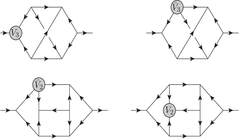
Figure 12: Six loop product primitive graphs.

11 Beyond five loops.

While our focus to this point has been on the five loop renormalization group functions, the next stage in studying (2.1) would be to extend this to six loops. Given what we have established here it is worth giving guidance on what would be required for that as several common features emerged. First, at six loops there are $324$ Feynman graphs contributing to the $\Phi$ $2$-point function. The content of $\gamma_{\Phi}(a)$ at that order will involve rationals as well as what we term irrationals. The majority of these will be $\zeta_{n}$ for $n$ $=$ $3$ to $9$. In addition their products such as $\zeta_{3}\zeta_{5}$ and $\zeta_{3}^{3}$, which are both present in the six loop $\phi^{4}$ $\beta$-function [32, 34], should appear if the structure of the renormalization group functions of this non-supersymmetric paradigm theory is valid. That would therefore imply the potential additional presence of the multiple zeta $\zeta_{3,5}$. As noted earlier the $O(1/N^{3})$ expression for the exponent $\eta$, [49], may indicate that such an irrational is actually absent. However if it were present it would have to arise in a primitive graph whose $O(N)$ group theory factor is beyond $O(1/N^{3})$. Alternatively candidate primitive graphs from $\phi^{4}$ theory may be excluded because of the restriction the chiral symmetry places on the graph topologies.

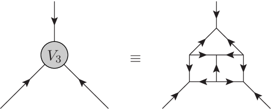
Figure 13: Three loop planar vertex correction.

Of the $324$ graphs it turns out that $17$ of these are primitive. One feature to emerge from the five loop evaluation of the Feynman graphs was the appearance of what was termed the product primitives. These are $2$-point graphs with vertex subgraphs. As the vertex function is finite, we noted that the simple pole can be deduced from the finite value of the vertex itself. At six loops we have illustrated the $8$ graphs of the total primitives that are product primitives in Figure 12 where the vertex $V_{3}$ is defined in Figure 13. The residue of the simple pole in $\epsilon$ of each of the graphs will be proportional to $\zeta_{3}\zeta_{5}$ and have a group factor of $T_{2}T_{5}T_{71}$ for (6.1). The explicit coefficient of this residue requires the implementation of the $D$-algebra. This is also an issue for the remaining non-product primitives especially as the power of the irreducible scalar products increases with loop order. The remaining graphs intermediate to those with rational contributions and the primitives correspond to the decoration of the lower loop primitives with an extra one loop bubble. A subset of these should be calculable with the use of subtractions and Forcer. The remainder of this type, similar to the non-product primitives, could only be reliably evaluated with a five loop version of Forcer.

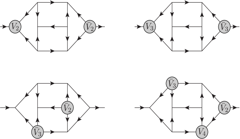
Figure 14: Higher order product primitive graphs.

Next we note that the concept of product primitives naturally continues at higher loop order. We have provided several examples in Figure 14 to illustrate the point. A new vertex function $V_{4}$ has been defined in Figure 15 where the actual $3$-point function is isolated by amputating the right external vertex. In Figure 14 the graphs are $8$, $10$, $9$ and $13$ loops respectively from top left to bottom right. The simple pole residue of each would be $\zeta_{3}^{2}\zeta_{5}$, $\zeta_{5}^{3}$, $\zeta_{3}\zeta_{5}^{2}$ and $\zeta_{3}\zeta_{5}^{2}\zeta_{7}$ in the same respective order with the equally associated group factors of $T_{2}T_{5}^{2}T_{71}$, $T_{2}T_{71}^{3}$, $T_{2}T_{5}T_{71}^{2}$ and $T_{2}T_{5}T_{71}^{2}T_{94}$. So there is a clear association of each group factor with a specific $\zeta_{n}$.

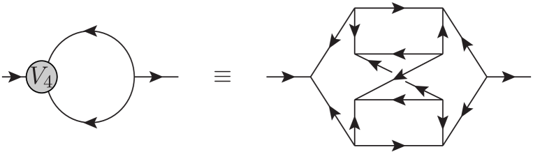
Figure 15: Definition of four loop primitive vertex.

Finally we return to the rational part of $\gamma_{\Phi}(a)$ and note that it is possible to deduce the contribution in the $\overline{\mbox{MS}}$ scheme purely from the five loop computation. This is because the rational part of the six loop MOM scheme is known from the Hopf algebra solution of the Dyson-Schwinger equation given in [81]. As we showed earlier the five loop MOM expression for $\gamma_{\Phi}(a)$ could be deduced from the $\overline{\mbox{MS}}$ expression by using the coupling constant map (5.6) and the formalism of (5.8) and (5.9). To extract the rational part at six loops requires one ingredient which is the finite part of the $\Phi$ $2$-point function at five loops. This is because the coupling constant mapping at $L$ loops determines the $(L+1)$ loop renormalization group functions from (5.8) and (5.9) once they are available at $L$ loops in one specific scheme. Previously the MOM five loop $\beta$-function was deduced from the $\overline{\mbox{MS}}$ one. Here we reverse the process given the result of [81]. So all that is required is the rational part of the $\Phi$ $2$-point function at five loops. As these are the bubble graphs which are simple to evaluate to the finite part we have applied the formalism to find the rational piece of the six loop $\overline{\mbox{MS}}$ $\beta$-function which is

$$\beta(a) = \frac{3}{2}a^{2}~{}-~{}\frac{3}{2}a^{3}~{}+~{}\left[36\zeta_{3}+15\right]\frac{a^{4}}{8}~{}+~{}\left[54\zeta_{4}-180\zeta_{3}-240\zeta_{5}-27\right]\frac{a^{5}}{8}$$ (11.1)

$$+~{}\left[1512\zeta_{3}^{2}+2574\zeta_{3}-1323\zeta_{4}+5484\zeta_{5}-2700\zeta_{6}+7938\zeta_{7}+237\right]\frac{a^{6}}{32}$$

$$+~{}\left[-~{}\frac{369}{20}~{}+~{}\mbox{non-rational contribution}\right]a^{7}~{}+~{}O(a^{8})$$

and we note that the alternating sign pattern of the rationals is maintained. To determine the non-rational contribution of (11.1) is of course a more strenuous exercise.

12 Discussion.

We have completed a comprehensive study of the Wess-Zumino model at five loops. This has proceeded in two phases with the initial one outlining the algorithm for carrying out the computation of the five loop Feynman graphs that are required for the $\beta$-function of the original model of [1]. Once established the second part addressed applications to various extensions of the core theory by allowing the fields to lie in various symmetry groups or take the couplings to be general tensors. One consequence was to extend the precision of the $\epsilon$ expansion of critical exponents to a new order. This is important in the context of other methods such as the conformal bootstrap and the functional renormalization group techniques. These have been applied to several problems like the emergent supersymmetric fixed point that is present in Gross-Neveu-Yukawa systems which relate to materials in Nature and could be the first manifestation of supersymmetry in reality. As a corollary the five loop Wess-Zumino renormalization could be a useful independent check on any future higher order renormalization of that system. However, to effect such a calculation in the Gross-Neveu-Yukawa model in four dimensions at five loops would be a massive undertaking especially given the number of graphs that would need to be evaluated. At four loops either $7384$ or $188531$ Feynman graphs were determined in [15] where the two totals depend on whether real or complex scalars were used together with their respective Dirac or left and right handed Weyl fermions. These are substantially larger numbers than the four loop ones given in Table 1. This is primarily due to the fact that unlike the component Wess-Zumino model each interaction of the Gross-Neveu-Yukawa system has an independent coupling constant. Consequently all the $3$- and $4$-point vertices have to be renormalized separately in the absence of any Ward identities. One interesting aspect of the $\epsilon$ expansion analysis was the close agreement of the five loop estimates with other methods for the Gross-Neveu-Yukawa system as is evident from Table 3. While the five loop results appear competitive with the latest bootstrap estimates there is still not precise agreement. Whether this is an indication of some discrepancy or not, such as non-perturbative contributions outside the scope of perturbation theory, is worth pursuing. If so it should not violate the underlying supersymmetry in the extension from four to three dimensions in an $\epsilon$ expansion approach. The other case where we produced exponent estimates to compare with bootstrap methods, which concerned the one dimensional conformal manifold connected to the XYZ model, we found values that in some instances were close to the values quoted in [40]. This suggests that perhaps higher orders in $\epsilon$ would be necessary to produce a more accurate comparison. While we have sketched out some basic ideas as to how a six loop computation could proceed again such a task is not trivial. Perhaps the graphical function methods of [31, 32, 33] offers the best direction to follow especially if the method could be adapted to superspace in the first instance rather than have to use a component Lagrangian. Such a six loop renormalization would give insight into whether there are multiple zetas in the $\beta$-function of the Wess-Zumino model. This is the order where $\zeta_{3,5}$ first appears in its non-supersymmetric cousin $\phi^{4}$ theory which also has no chiral symmetry. If it was present at this order in (2.1) then there would be no more debate.

Acknowledgements. We thank I. Jack for useful discussions at various stages of this work, H. Osborn for pointing out reference [40], D. Poland for discussions on the conformal bootstrap formalism as well as G. Dunne for posing several questions. It is also a pleasure to thank D.J. Broadhurst for enlightening discussions over many years concerning multiple zetas in primitive Feynman integrals at very high loop order. This work was supported by a DFG Mercator Fellowship and in part through the STFC Consolidated Grants ST/J000493/1 and ST/T000988/1. The graphs were drawn with the Axodraw package [105].

Appendix A Tensor definitions.

In this appendix we define the tensors $T_{Lr}^{ij}$ that appear in the anomalous dimension of the general action (9.1). Each of these tensors depends on the tensor couplings $d^{ijk}$ and $\bar{d}^{ijk}$. The subscript of each dummy index $j_{n}$ in each of the definitions is in direct correspondence to the label used in the Qgraf electronic output that defines the underlying graph. In particular the bridge between $T_{Lr}^{ij}$ and the settings of the qgraf.dat file in partnership with the form.sty style file is to use the notadp and onepi options. To three loops the first set of tensors is

$$d^{ij_{1}j_{2}}\bar{d}^{jj_{1}j_{2}}~{}=~{}T_{11}^{ij}$$

$$d^{ij_{1}j_{2}}d^{j_{3}j_{4}j_{5}}\bar{d}^{jj_{1}j_{3}}\bar{d}^{j_{2}j_{4}j_{5}}~{}=~{}T_{21}^{ij}$$

$$d^{ij_{1}j_{2}}d^{j_{3}j_{5}j_{7}}d^{j_{4}j_{6}j_{8}}\bar{d}^{jj_{3}j_{4}}\bar{d}^{j_{1}j_{5}j_{6}}\bar{d}^{j_{2}j_{7}j_{8}}~{}=~{}T_{31}^{ij}$$

$$d^{ij_{1}j_{2}}d^{j_{3}j_{5}j_{6}}d^{j_{4}j_{7}j_{8}}\bar{d}^{jj_{3}j_{4}}\bar{d}^{j_{1}j_{5}j_{6}}\bar{d}^{j_{2}j_{7}j_{8}}~{}=~{}T_{32}^{ij}$$

$$d^{ij_{1}j_{2}}d^{j_{3}j_{6}j_{7}}d^{j_{4}j_{5}j_{8}}\bar{d}^{jj_{1}j_{3}}\bar{d}^{j_{2}j_{4}j_{5}}\bar{d}^{j_{8}j_{6}j_{7}}~{}=~{}T_{33}^{ij}$$

$$d^{ij_{1}j_{2}}d^{j_{3}j_{4}j_{6}}d^{j_{5}j_{7}j_{8}}\bar{d}^{jj_{1}j_{3}}\bar{d}^{j_{2}j_{4}j_{5}}\bar{d}^{j_{6}j_{7}j_{8}}~{}=~{}T_{34}^{ij}~{}.$$ (A.1)

For orientation $T_{11}^{ij}$ and $T_{21}^{ij}$ correspond to the graphs of Figures 1 and 2 respectively while $T_{31}^{ij}$ is the non-planar graph of Figure 4. We note that in [91] a factor of $\frac{1}{2}$ was included in the definition of the tensor corresponding to $T_{11}^{ij}$. At four loops the $13$ tensors are

$$d^{ij_{1}j_{2}}d^{j_{3}j_{5}j_{9}}d^{j_{4}j_{7}j_{10}}d^{j_{6}j_{8}j_{11}}\bar{d}^{jj_{3}j_{4}}\bar{d}^{j_{1}j_{5}j_{6}}\bar{d}^{j_{2}j_{7}j_{8}}\bar{d}^{j_{9}j_{10}j_{11}}~{}=~{}T_{41}^{ij}$$

$$d^{ij_{1}j_{2}}d^{j_{3}j_{5}j_{9}}d^{j_{4}j_{6}j_{10}}d^{j_{11}j_{7}j_{8}}\bar{d}^{jj_{3}j_{4}}\bar{d}^{j_{1}j_{5}j_{6}}\bar{d}^{j_{2}j_{7}j_{8}}\bar{d}^{j_{9}j_{10}j_{11}}~{}=~{}T_{42}^{ij}$$

$$d^{ij_{3}j_{4}}d^{j_{1}j_{5}j_{6}}d^{j_{2}j_{7}j_{8}}d^{j_{9}j_{10}j_{11}}\bar{d}^{jj_{1}j_{2}}\bar{d}^{j_{3}j_{5}j_{9}}\bar{d}^{j_{4}j_{6}j_{10}}\bar{d}^{j_{11}j_{7}j_{8}}~{}=~{}T_{43}^{ij}$$

$$d^{ij_{1}j_{2}}d^{j_{3}j_{5}j_{7}}d^{j_{4}j_{6}j_{9}}d^{j_{8}j_{10}j_{11}}\bar{d}^{jj_{3}j_{4}}\bar{d}^{j_{1}j_{5}j_{6}}\bar{d}^{j_{2}j_{7}j_{8}}\bar{d}^{j_{9}j_{10}j_{11}}~{}=~{}T_{44}^{ij}$$

$$d^{ij_{1}j_{2}}d^{j_{3}j_{5}j_{6}}d^{j_{4}j_{9}j_{10}}d^{j_{7}j_{8}j_{11}}\bar{d}^{jj_{3}j_{4}}\bar{d}^{j_{1}j_{5}j_{6}}\bar{d}^{j_{2}j_{7}j_{8}}\bar{d}^{j_{11}j_{9}j_{10}}~{}=~{}T_{45}^{ij}$$

$$d^{ij_{1}j_{2}}d^{j_{3}j_{5}j_{6}}d^{j_{4}j_{7}j_{9}}d^{j_{8}j_{10}j_{11}}\bar{d}^{jj_{3}j_{4}}\bar{d}^{j_{1}j_{5}j_{6}}\bar{d}^{j_{2}j_{7}j_{8}}\bar{d}^{j_{9}j_{10}j_{11}}~{}=~{}T_{46}^{ij}$$

$$d^{ij_{1}j_{2}}d^{j_{3}j_{6}j_{7}}d^{j_{4}j_{8}j_{9}}d^{j_{5}j_{10}j_{11}}\bar{d}^{jj_{1}j_{3}}\bar{d}^{j_{2}j_{4}j_{5}}\bar{d}^{j_{6}j_{8}j_{10}}\bar{d}^{j_{7}j_{9}j_{11}}~{}=~{}T_{47}^{ij}$$

$$d^{ij_{1}j_{2}}d^{j_{3}j_{6}j_{7}}d^{j_{4}j_{8}j_{9}}d^{j_{5}j_{10}j_{11}}\bar{d}^{jj_{1}j_{3}}\bar{d}^{j_{2}j_{4}j_{5}}\bar{d}^{j_{6}j_{8}j_{9}}\bar{d}^{j_{7}j_{10}j_{11}}~{}=~{}T_{48}^{ij}$$

$$d^{ij_{1}j_{2}}d^{j_{3}j_{6}j_{7}}d^{j_{4}j_{5}j_{8}}d^{j_{9}j_{10}j_{11}}\bar{d}^{jj_{1}j_{3}}\bar{d}^{j_{2}j_{4}j_{5}}\bar{d}^{j_{7}j_{10}j_{11}}\bar{d}^{j_{8}j_{6}j_{9}}~{}=~{}T_{49}^{ij}$$

$$d^{ij_{1}j_{3}}d^{j_{2}j_{4}j_{5}}d^{j_{7}j_{10}j_{11}}d^{j_{8}j_{6}j_{9}}\bar{d}^{jj_{1}j_{2}}\bar{d}^{j_{3}j_{6}j_{7}}\bar{d}^{j_{4}j_{5}j_{8}}\bar{d}^{j_{9}j_{10}j_{11}}~{}=~{}T_{410}^{ij}$$

$$d^{ij_{1}j_{2}}d^{j_{3}j_{6}j_{7}}d^{j_{4}j_{5}j_{8}}d^{j_{9}j_{10}j_{11}}\bar{d}^{jj_{1}j_{3}}\bar{d}^{j_{2}j_{4}j_{5}}\bar{d}^{j_{6}j_{7}j_{9}}\bar{d}^{j_{8}j_{10}j_{11}}~{}=~{}T_{411}^{ij}$$

$$d^{ij_{1}j_{2}}d^{j_{3}j_{4}j_{6}}d^{j_{5}j_{7}j_{8}}d^{j_{11}j_{9}j_{10}}\bar{d}^{jj_{1}j_{3}}\bar{d}^{j_{2}j_{4}j_{5}}\bar{d}^{j_{6}j_{9}j_{10}}\bar{d}^{j_{7}j_{8}j_{11}}~{}=~{}T_{412}^{ij}$$

$$d^{ij_{1}j_{2}}d^{j_{3}j_{4}j_{6}}d^{j_{5}j_{7}j_{8}}d^{j_{9}j_{10}j_{11}}\bar{d}^{jj_{1}j_{3}}\bar{d}^{j_{2}j_{4}j_{5}}\bar{d}^{j_{6}j_{7}j_{9}}\bar{d}^{j_{8}j_{10}j_{11}}~{}=~{}T_{413}^{ij}$$ (A.2)

where $T_{44}^{ij}$ and $T_{41}^{ij}$ respectively correspond to the graphs in the bottom row of Figure 6.

At five loops the $63$ different tensors are

$$d^{ij_{1}j_{2}}d^{j_{3}j_{9}j_{10}}d^{j_{4}j_{11}j_{12}}d^{j_{5}j_{7}j_{13}}d^{j_{6}j_{8}j_{14}}\bar{d}^{jj_{3}j_{4}}\bar{d}^{j_{1}j_{5}j_{6}}\bar{d}^{j_{2}j_{7}j_{8}}\bar{d}^{j_{13}j_{9}j_{11}}\bar{d}^{j_{14}j_{10}j_{12}}~{}=~{}T_{51}^{ij}$$

$$d^{ij_{1}j_{2}}d^{j_{3}j_{9}j_{10}}d^{j_{4}j_{11}j_{12}}d^{j_{5}j_{6}j_{13}}d^{j_{7}j_{8}j_{14}}\bar{d}^{jj_{3}j_{4}}\bar{d}^{j_{1}j_{5}j_{6}}\bar{d}^{j_{2}j_{7}j_{8}}\bar{d}^{j_{13}j_{9}j_{11}}\bar{d}^{j_{14}j_{10}j_{12}}~{}=~{}T_{52}^{ij}$$

$$d^{ij_{3}j_{4}}d^{j_{1}j_{5}j_{6}}d^{j_{2}j_{7}j_{8}}d^{j_{13}j_{9}j_{11}}d^{j_{14}j_{10}j_{12}}\bar{d}^{jj_{1}j_{2}}\bar{d}^{j_{3}j_{9}j_{10}}\bar{d}^{j_{4}j_{11}j_{12}}\bar{d}^{j_{5}j_{6}j_{13}}\bar{d}^{j_{7}j_{8}j_{14}}~{}=~{}T_{53}^{ij}$$

$$d^{ij_{1}j_{2}}d^{j_{3}j_{9}j_{10}}d^{j_{4}j_{11}j_{12}}d^{j_{5}j_{6}j_{13}}d^{j_{7}j_{8}j_{14}}\bar{d}^{jj_{3}j_{4}}\bar{d}^{j_{1}j_{5}j_{6}}\bar{d}^{j_{2}j_{7}j_{8}}\bar{d}^{j_{13}j_{9}j_{10}}\bar{d}^{j_{14}j_{11}j_{12}}~{}=~{}T_{54}^{ij}$$

$$d^{ij_{1}j_{2}}d^{j_{3}j_{5}j_{9}}d^{j_{4}j_{10}j_{11}}d^{j_{6}j_{12}j_{13}}d^{j_{7}j_{8}j_{14}}\bar{d}^{jj_{3}j_{4}}\bar{d}^{j_{1}j_{5}j_{6}}\bar{d}^{j_{2}j_{7}j_{8}}\bar{d}^{j_{9}j_{14}j_{12}}\bar{d}^{j_{13}j_{10}j_{11}}~{}=~{}T_{55}^{ij}$$

$$d^{ij_{1}j_{2}}d^{j_{3}j_{5}j_{9}}d^{j_{4}j_{10}j_{11}}d^{j_{6}j_{12}j_{13}}d^{j_{7}j_{8}j_{14}}\bar{d}^{jj_{3}j_{4}}\bar{d}^{j_{1}j_{5}j_{6}}\bar{d}^{j_{2}j_{7}j_{8}}\bar{d}^{j_{9}j_{12}j_{13}}\bar{d}^{j_{14}j_{10}j_{11}}~{}=~{}T_{56}^{ij}$$

$$d^{ij_{1}j_{2}}d^{j_{3}j_{5}j_{9}}d^{j_{4}j_{10}j_{11}}d^{j_{6}j_{7}j_{12}}d^{j_{8}j_{13}j_{14}}\bar{d}^{jj_{3}j_{4}}\bar{d}^{j_{1}j_{5}j_{6}}\bar{d}^{j_{2}j_{7}j_{8}}\bar{d}^{j_{9}j_{13}j_{14}}\bar{d}^{j_{12}j_{10}j_{11}}~{}=~{}T_{57}^{ij}$$

$$d^{ij_{3}j_{4}}d^{j_{1}j_{5}j_{6}}d^{j_{2}j_{7}j_{8}}d^{j_{9}j_{13}j_{14}}d^{j_{12}j_{10}j_{11}}\bar{d}^{jj_{1}j_{2}}\bar{d}^{j_{3}j_{5}j_{9}}\bar{d}^{j_{4}j_{10}j_{11}}\bar{d}^{j_{6}j_{7}j_{12}}\bar{d}^{j_{8}j_{13}j_{14}}~{}=~{}T_{58}^{ij}$$

$$d^{ij_{1}j_{2}}d^{j_{3}j_{5}j_{9}}d^{j_{4}j_{10}j_{11}}d^{j_{6}j_{7}j_{12}}d^{j_{8}j_{13}j_{14}}\bar{d}^{jj_{3}j_{4}}\bar{d}^{j_{1}j_{5}j_{6}}\bar{d}^{j_{2}j_{7}j_{8}}\bar{d}^{j_{9}j_{12}j_{13}}\bar{d}^{j_{14}j_{10}j_{11}}~{}=~{}T_{59}^{ij}$$

$$d^{ij_{3}j_{4}}d^{j_{1}j_{5}j_{6}}d^{j_{2}j_{7}j_{8}}d^{j_{9}j_{12}j_{13}}d^{j_{14}j_{10}j_{11}}\bar{d}^{jj_{1}j_{2}}\bar{d}^{j_{3}j_{5}j_{9}}\bar{d}^{j_{4}j_{10}j_{11}}\bar{d}^{j_{6}j_{7}j_{12}}\bar{d}^{j_{8}j_{13}j_{14}}~{}=~{}T_{510}^{ij}$$

$$d^{ij_{1}j_{2}}d^{j_{3}j_{5}j_{9}}d^{j_{4}j_{10}j_{11}}d^{j_{6}j_{7}j_{12}}d^{j_{8}j_{13}j_{14}}\bar{d}^{jj_{3}j_{4}}\bar{d}^{j_{1}j_{5}j_{6}}\bar{d}^{j_{2}j_{7}j_{8}}\bar{d}^{j_{9}j_{10}j_{13}}\bar{d}^{j_{12}j_{11}j_{14}}~{}=~{}T_{511}^{ij}$$

$$d^{ij_{1}j_{2}}d^{j_{3}j_{5}j_{9}}d^{j_{4}j_{10}j_{11}}d^{j_{6}j_{7}j_{12}}d^{j_{8}j_{13}j_{14}}\bar{d}^{jj_{3}j_{4}}\bar{d}^{j_{1}j_{5}j_{6}}\bar{d}^{j_{2}j_{7}j_{8}}\bar{d}^{j_{9}j_{12}j_{10}}\bar{d}^{j_{11}j_{13}j_{14}}~{}=~{}T_{512}^{ij}$$

$$d^{ij_{1}j_{2}}d^{j_{3}j_{5}j_{9}}d^{j_{4}j_{7}j_{10}}d^{j_{6}j_{11}j_{12}}d^{j_{8}j_{13}j_{14}}\bar{d}^{jj_{3}j_{4}}\bar{d}^{j_{1}j_{5}j_{6}}\bar{d}^{j_{2}j_{7}j_{8}}\bar{d}^{j_{9}j_{13}j_{14}}\bar{d}^{j_{10}j_{11}j_{12}}~{}=~{}T_{513}^{ij}$$

$$d^{ij_{1}j_{2}}d^{j_{3}j_{5}j_{9}}d^{j_{4}j_{7}j_{10}}d^{j_{6}j_{11}j_{12}}d^{j_{8}j_{13}j_{14}}\bar{d}^{jj_{3}j_{4}}\bar{d}^{j_{1}j_{5}j_{6}}\bar{d}^{j_{2}j_{7}j_{8}}\bar{d}^{j_{9}j_{11}j_{13}}\bar{d}^{j_{10}j_{12}j_{14}}~{}=~{}T_{514}^{ij}$$

$$d^{ij_{1}j_{2}}d^{j_{3}j_{5}j_{9}}d^{j_{4}j_{7}j_{10}}d^{j_{6}j_{11}j_{12}}d^{j_{8}j_{13}j_{14}}\bar{d}^{jj_{3}j_{4}}\bar{d}^{j_{1}j_{5}j_{6}}\bar{d}^{j_{2}j_{7}j_{8}}\bar{d}^{j_{9}j_{11}j_{12}}\bar{d}^{j_{10}j_{13}j_{14}}~{}=~{}T_{515}^{ij}$$

$$d^{ij_{1}j_{2}}d^{j_{3}j_{5}j_{9}}d^{j_{4}j_{7}j_{10}}d^{j_{6}j_{8}j_{11}}d^{j_{12}j_{13}j_{14}}\bar{d}^{jj_{3}j_{4}}\bar{d}^{j_{1}j_{5}j_{6}}\bar{d}^{j_{2}j_{7}j_{8}}\bar{d}^{j_{9}j_{11}j_{12}}\bar{d}^{j_{10}j_{13}j_{14}}~{}=~{}T_{516}^{ij}$$

$$d^{ij_{3}j_{4}}d^{j_{1}j_{5}j_{6}}d^{j_{2}j_{7}j_{8}}d^{j_{9}j_{11}j_{12}}d^{j_{10}j_{13}j_{14}}\bar{d}^{jj_{1}j_{2}}\bar{d}^{j_{3}j_{5}j_{9}}\bar{d}^{j_{4}j_{7}j_{10}}\bar{d}^{j_{6}j_{8}j_{11}}\bar{d}^{j_{12}j_{13}j_{14}}~{}=~{}T_{517}^{ij}$$

$$d^{ij_{1}j_{2}}d^{j_{3}j_{5}j_{9}}d^{j_{4}j_{7}j_{10}}d^{j_{6}j_{8}j_{11}}d^{j_{12}j_{13}j_{14}}\bar{d}^{jj_{3}j_{4}}\bar{d}^{j_{1}j_{5}j_{6}}\bar{d}^{j_{2}j_{7}j_{8}}\bar{d}^{j_{9}j_{10}j_{12}}\bar{d}^{j_{11}j_{13}j_{14}}~{}=~{}T_{518}^{ij}$$

$$d^{ij_{1}j_{2}}d^{j_{3}j_{5}j_{9}}d^{j_{4}j_{6}j_{10}}d^{j_{7}j_{11}j_{12}}d^{j_{8}j_{13}j_{14}}\bar{d}^{jj_{3}j_{4}}\bar{d}^{j_{1}j_{5}j_{6}}\bar{d}^{j_{2}j_{7}j_{8}}\bar{d}^{j_{9}j_{11}j_{13}}\bar{d}^{j_{10}j_{12}j_{14}}~{}=~{}T_{519}^{ij}$$

$$d^{ij_{3}j_{4}}d^{j_{1}j_{5}j_{6}}d^{j_{2}j_{7}j_{8}}d^{j_{9}j_{11}j_{13}}d^{j_{10}j_{12}j_{14}}\bar{d}^{jj_{1}j_{2}}\bar{d}^{j_{3}j_{5}j_{9}}\bar{d}^{j_{4}j_{6}j_{10}}\bar{d}^{j_{7}j_{11}j_{12}}\bar{d}^{j_{8}j_{13}j_{14}}~{}=~{}T_{520}^{ij}$$

$$d^{ij_{1}j_{2}}d^{j_{3}j_{5}j_{9}}d^{j_{4}j_{6}j_{10}}d^{j_{7}j_{11}j_{12}}d^{j_{8}j_{13}j_{14}}\bar{d}^{jj_{3}j_{4}}\bar{d}^{j_{1}j_{5}j_{6}}\bar{d}^{j_{2}j_{7}j_{8}}\bar{d}^{j_{9}j_{11}j_{12}}\bar{d}^{j_{10}j_{13}j_{14}}~{}=~{}T_{521}^{ij}$$

$$d^{ij_{3}j_{4}}d^{j_{1}j_{5}j_{6}}d^{j_{2}j_{7}j_{8}}d^{j_{9}j_{11}j_{12}}d^{j_{10}j_{13}j_{14}}\bar{d}^{jj_{1}j_{2}}\bar{d}^{j_{3}j_{5}j_{9}}\bar{d}^{j_{4}j_{6}j_{10}}\bar{d}^{j_{7}j_{11}j_{12}}\bar{d}^{j_{8}j_{13}j_{14}}~{}=~{}T_{522}^{ij}$$

$$d^{ij_{1}j_{2}}d^{j_{3}j_{5}j_{9}}d^{j_{4}j_{6}j_{10}}d^{j_{8}j_{13}j_{14}}d^{j_{11}j_{7}j_{12}}\bar{d}^{jj_{3}j_{4}}\bar{d}^{j_{1}j_{5}j_{6}}\bar{d}^{j_{2}j_{7}j_{8}}\bar{d}^{j_{9}j_{10}j_{11}}\bar{d}^{j_{12}j_{13}j_{14}}~{}=~{}T_{523}^{ij}$$

$$d^{ij_{3}j_{4}}d^{j_{1}j_{5}j_{6}}d^{j_{2}j_{7}j_{8}}d^{j_{9}j_{10}j_{11}}d^{j_{12}j_{13}j_{14}}\bar{d}^{jj_{1}j_{2}}\bar{d}^{j_{3}j_{5}j_{9}}\bar{d}^{j_{4}j_{6}j_{10}}\bar{d}^{j_{8}j_{13}j_{14}}\bar{d}^{j_{11}j_{7}j_{12}}~{}=~{}T_{524}^{ij}$$

$$d^{ij_{1}j_{2}}d^{j_{3}j_{5}j_{9}}d^{j_{4}j_{6}j_{10}}d^{j_{7}j_{8}j_{11}}d^{j_{12}j_{13}j_{14}}\bar{d}^{jj_{3}j_{4}}\bar{d}^{j_{1}j_{5}j_{6}}\bar{d}^{j_{2}j_{7}j_{8}}\bar{d}^{j_{9}j_{11}j_{12}}\bar{d}^{j_{10}j_{13}j_{14}}~{}=~{}T_{525}^{ij}$$

$$d^{ij_{3}j_{4}}d^{j_{1}j_{5}j_{6}}d^{j_{2}j_{7}j_{8}}d^{j_{9}j_{11}j_{12}}d^{j_{10}j_{13}j_{14}}\bar{d}^{jj_{1}j_{2}}\bar{d}^{j_{3}j_{5}j_{9}}\bar{d}^{j_{4}j_{6}j_{10}}\bar{d}^{j_{7}j_{8}j_{11}}\bar{d}^{j_{12}j_{13}j_{14}}~{}=~{}T_{526}^{ij}$$

$$d^{ij_{1}j_{2}}d^{j_{3}j_{5}j_{9}}d^{j_{4}j_{6}j_{10}}d^{j_{7}j_{8}j_{11}}d^{j_{12}j_{13}j_{14}}\bar{d}^{jj_{3}j_{4}}\bar{d}^{j_{1}j_{5}j_{6}}\bar{d}^{j_{2}j_{7}j_{8}}\bar{d}^{j_{9}j_{10}j_{12}}\bar{d}^{j_{11}j_{13}j_{14}}~{}=~{}T_{527}^{ij}$$

$$d^{ij_{3}j_{4}}d^{j_{1}j_{5}j_{6}}d^{j_{2}j_{7}j_{8}}d^{j_{9}j_{10}j_{12}}d^{j_{11}j_{13}j_{14}}\bar{d}^{jj_{1}j_{2}}\bar{d}^{j_{3}j_{5}j_{9}}\bar{d}^{j_{4}j_{6}j_{10}}\bar{d}^{j_{7}j_{8}j_{11}}\bar{d}^{j_{12}j_{13}j_{14}}~{}=~{}T_{528}^{ij}$$

$$d^{ij_{1}j_{2}}d^{j_{3}j_{5}j_{7}}d^{j_{4}j_{6}j_{9}}d^{j_{8}j_{10}j_{11}}d^{j_{14}j_{12}j_{13}}\bar{d}^{jj_{3}j_{4}}\bar{d}^{j_{1}j_{5}j_{6}}\bar{d}^{j_{2}j_{7}j_{8}}\bar{d}^{j_{9}j_{12}j_{13}}\bar{d}^{j_{10}j_{11}j_{14}}~{}=~{}T_{529}^{ij}$$

$$d^{ij_{1}j_{2}}d^{j_{3}j_{5}j_{7}}d^{j_{4}j_{6}j_{9}}d^{j_{8}j_{10}j_{11}}d^{j_{12}j_{13}j_{14}}\bar{d}^{jj_{3}j_{4}}\bar{d}^{j_{1}j_{5}j_{6}}\bar{d}^{j_{2}j_{7}j_{8}}\bar{d}^{j_{9}j_{10}j_{12}}\bar{d}^{j_{11}j_{13}j_{14}}~{}=~{}T_{530}^{ij}$$

$$d^{ij_{1}j_{2}}d^{j_{3}j_{5}j_{6}}d^{j_{4}j_{9}j_{10}}d^{j_{7}j_{11}j_{12}}d^{j_{8}j_{13}j_{14}}\bar{d}^{jj_{3}j_{4}}\bar{d}^{j_{1}j_{5}j_{6}}\bar{d}^{j_{2}j_{7}j_{8}}\bar{d}^{j_{9}j_{11}j_{13}}\bar{d}^{j_{10}j_{12}j_{14}}~{}=~{}T_{531}^{ij}$$

$$d^{ij_{1}j_{2}}d^{j_{3}j_{5}j_{6}}d^{j_{4}j_{9}j_{10}}d^{j_{7}j_{11}j_{12}}d^{j_{8}j_{13}j_{14}}\bar{d}^{jj_{3}j_{4}}\bar{d}^{j_{1}j_{5}j_{6}}\bar{d}^{j_{2}j_{7}j_{8}}\bar{d}^{j_{9}j_{11}j_{12}}\bar{d}^{j_{10}j_{13}j_{14}}~{}=~{}T_{532}^{ij}$$

$$d^{ij_{1}j_{2}}d^{j_{3}j_{5}j_{6}}d^{j_{4}j_{9}j_{10}}d^{j_{7}j_{8}j_{11}}d^{j_{12}j_{13}j_{14}}\bar{d}^{jj_{3}j_{4}}\bar{d}^{j_{1}j_{5}j_{6}}\bar{d}^{j_{2}j_{7}j_{8}}\bar{d}^{j_{10}j_{13}j_{14}}\bar{d}^{j_{11}j_{9}j_{12}}~{}=~{}T_{533}^{ij}$$

$$d^{ij_{3}j_{4}}d^{j_{1}j_{5}j_{6}}d^{j_{2}j_{7}j_{8}}d^{j_{10}j_{13}j_{14}}d^{j_{11}j_{9}j_{12}}\bar{d}^{jj_{1}j_{2}}\bar{d}^{j_{3}j_{5}j_{6}}\bar{d}^{j_{4}j_{9}j_{10}}\bar{d}^{j_{7}j_{8}j_{11}}\bar{d}^{j_{12}j_{13}j_{14}}~{}=~{}T_{534}^{ij}$$

$$d^{ij_{1}j_{2}}d^{j_{3}j_{5}j_{6}}d^{j_{4}j_{9}j_{10}}d^{j_{7}j_{8}j_{11}}d^{j_{12}j_{13}j_{14}}\bar{d}^{jj_{3}j_{4}}\bar{d}^{j_{1}j_{5}j_{6}}\bar{d}^{j_{2}j_{7}j_{8}}\bar{d}^{j_{9}j_{10}j_{12}}\bar{d}^{j_{11}j_{13}j_{14}}~{}=~{}T_{535}^{ij}$$

$$d^{ij_{1}j_{2}}d^{j_{3}j_{5}j_{6}}d^{j_{4}j_{7}j_{9}}d^{j_{8}j_{10}j_{11}}d^{j_{14}j_{12}j_{13}}\bar{d}^{jj_{3}j_{4}}\bar{d}^{j_{1}j_{5}j_{6}}\bar{d}^{j_{2}j_{7}j_{8}}\bar{d}^{j_{9}j_{12}j_{13}}\bar{d}^{j_{10}j_{11}j_{14}}~{}=~{}T_{536}^{ij}$$

$$d^{ij_{1}j_{2}}d^{j_{3}j_{5}j_{6}}d^{j_{4}j_{7}j_{9}}d^{j_{8}j_{10}j_{11}}d^{j_{12}j_{13}j_{14}}\bar{d}^{jj_{3}j_{4}}\bar{d}^{j_{1}j_{5}j_{6}}\bar{d}^{j_{2}j_{7}j_{8}}\bar{d}^{j_{9}j_{10}j_{12}}\bar{d}^{j_{11}j_{13}j_{14}}~{}=~{}T_{537}^{ij}$$

$$d^{ij_{1}j_{2}}d^{j_{3}j_{6}j_{7}}d^{j_{4}j_{8}j_{9}}d^{j_{5}j_{10}j_{11}}d^{j_{12}j_{13}j_{14}}\bar{d}^{jj_{1}j_{3}}\bar{d}^{j_{2}j_{4}j_{5}}\bar{d}^{j_{6}j_{8}j_{12}}\bar{d}^{j_{7}j_{13}j_{14}}\bar{d}^{j_{9}j_{10}j_{11}}~{}=~{}T_{538}^{ij}$$

$$d^{ij_{1}j_{2}}d^{j_{3}j_{6}j_{7}}d^{j_{4}j_{8}j_{9}}d^{j_{5}j_{10}j_{11}}d^{j_{12}j_{13}j_{14}}\bar{d}^{jj_{1}j_{3}}\bar{d}^{j_{2}j_{4}j_{5}}\bar{d}^{j_{6}j_{8}j_{12}}\bar{d}^{j_{7}j_{10}j_{13}}\bar{d}^{j_{9}j_{11}j_{14}}~{}=~{}T_{539}^{ij}$$

$$d^{ij_{1}j_{2}}d^{j_{3}j_{6}j_{7}}d^{j_{4}j_{8}j_{9}}d^{j_{5}j_{10}j_{11}}d^{j_{12}j_{13}j_{14}}\bar{d}^{jj_{1}j_{3}}\bar{d}^{j_{2}j_{4}j_{5}}\bar{d}^{j_{6}j_{8}j_{12}}\bar{d}^{j_{7}j_{9}j_{13}}\bar{d}^{j_{14}j_{10}j_{11}}~{}=~{}T_{540}^{ij}$$

$$d^{ij_{1}j_{3}}d^{j_{2}j_{4}j_{5}}d^{j_{6}j_{8}j_{12}}d^{j_{7}j_{9}j_{13}}d^{j_{14}j_{10}j_{11}}\bar{d}^{jj_{1}j_{2}}\bar{d}^{j_{3}j_{6}j_{7}}\bar{d}^{j_{4}j_{8}j_{9}}\bar{d}^{j_{5}j_{10}j_{11}}\bar{d}^{j_{12}j_{13}j_{14}}~{}=~{}T_{541}^{ij}$$

$$d^{ij_{1}j_{2}}d^{j_{3}j_{6}j_{7}}d^{j_{4}j_{8}j_{9}}d^{j_{5}j_{10}j_{11}}d^{j_{12}j_{13}j_{14}}\bar{d}^{jj_{1}j_{3}}\bar{d}^{j_{2}j_{4}j_{5}}\bar{d}^{j_{6}j_{8}j_{10}}\bar{d}^{j_{7}j_{9}j_{12}}\bar{d}^{j_{11}j_{13}j_{14}}~{}=~{}T_{542}^{ij}$$

$$d^{ij_{1}j_{2}}d^{j_{3}j_{6}j_{7}}d^{j_{4}j_{8}j_{9}}d^{j_{5}j_{10}j_{11}}d^{j_{14}j_{12}j_{13}}\bar{d}^{jj_{1}j_{3}}\bar{d}^{j_{2}j_{4}j_{5}}\bar{d}^{j_{6}j_{8}j_{9}}\bar{d}^{j_{7}j_{12}j_{13}}\bar{d}^{j_{10}j_{11}j_{14}}~{}=~{}T_{543}^{ij}$$

$$d^{ij_{1}j_{2}}d^{j_{3}j_{6}j_{7}}d^{j_{4}j_{8}j_{9}}d^{j_{5}j_{10}j_{11}}d^{j_{12}j_{13}j_{14}}\bar{d}^{jj_{1}j_{3}}\bar{d}^{j_{2}j_{4}j_{5}}\bar{d}^{j_{6}j_{8}j_{9}}\bar{d}^{j_{7}j_{10}j_{12}}\bar{d}^{j_{11}j_{13}j_{14}}~{}=~{}T_{544}^{ij}$$

$$d^{ij_{1}j_{2}}d^{j_{3}j_{6}j_{7}}d^{j_{4}j_{5}j_{8}}d^{j_{9}j_{11}j_{13}}d^{j_{10}j_{12}j_{14}}\bar{d}^{jj_{1}j_{3}}\bar{d}^{j_{2}j_{4}j_{5}}\bar{d}^{j_{6}j_{9}j_{10}}\bar{d}^{j_{7}j_{11}j_{12}}\bar{d}^{j_{8}j_{13}j_{14}}~{}=~{}T_{545}^{ij}$$

$$d^{ij_{1}j_{3}}d^{j_{2}j_{4}j_{5}}d^{j_{6}j_{9}j_{10}}d^{j_{7}j_{11}j_{12}}d^{j_{8}j_{13}j_{14}}\bar{d}^{jj_{1}j_{2}}\bar{d}^{j_{3}j_{6}j_{7}}\bar{d}^{j_{4}j_{5}j_{8}}\bar{d}^{j_{9}j_{11}j_{13}}\bar{d}^{j_{10}j_{12}j_{14}}~{}=~{}T_{546}^{ij}$$

$$d^{ij_{1}j_{2}}d^{j_{3}j_{6}j_{7}}d^{j_{4}j_{5}j_{8}}d^{j_{9}j_{10}j_{13}}d^{j_{14}j_{11}j_{12}}\bar{d}^{jj_{1}j_{3}}\bar{d}^{j_{2}j_{4}j_{5}}\bar{d}^{j_{6}j_{9}j_{10}}\bar{d}^{j_{7}j_{11}j_{12}}\bar{d}^{j_{8}j_{13}j_{14}}~{}=~{}T_{547}^{ij}$$

$$d^{ij_{1}j_{3}}d^{j_{2}j_{4}j_{5}}d^{j_{6}j_{9}j_{10}}d^{j_{7}j_{11}j_{12}}d^{j_{8}j_{13}j_{14}}\bar{d}^{jj_{1}j_{2}}\bar{d}^{j_{3}j_{6}j_{7}}\bar{d}^{j_{4}j_{5}j_{8}}\bar{d}^{j_{9}j_{10}j_{13}}\bar{d}^{j_{14}j_{11}j_{12}}~{}=~{}T_{548}^{ij}$$

$$d^{ij_{1}j_{2}}d^{j_{3}j_{6}j_{7}}d^{j_{4}j_{5}j_{8}}d^{j_{9}j_{10}j_{11}}d^{j_{12}j_{13}j_{14}}\bar{d}^{jj_{1}j_{3}}\bar{d}^{j_{2}j_{4}j_{5}}\bar{d}^{j_{6}j_{9}j_{10}}\bar{d}^{j_{7}j_{11}j_{12}}\bar{d}^{j_{8}j_{13}j_{14}}~{}=~{}T_{549}^{ij}$$

$$d^{ij_{1}j_{3}}d^{j_{2}j_{4}j_{5}}d^{j_{6}j_{9}j_{10}}d^{j_{7}j_{11}j_{12}}d^{j_{8}j_{13}j_{14}}\bar{d}^{jj_{1}j_{2}}\bar{d}^{j_{3}j_{6}j_{7}}\bar{d}^{j_{4}j_{5}j_{8}}\bar{d}^{j_{9}j_{10}j_{11}}\bar{d}^{j_{12}j_{13}j_{14}}~{}=~{}T_{550}^{ij}$$

$$d^{ij_{1}j_{2}}d^{j_{3}j_{6}j_{7}}d^{j_{4}j_{5}j_{8}}d^{j_{9}j_{12}j_{13}}d^{j_{10}j_{11}j_{14}}\bar{d}^{jj_{1}j_{3}}\bar{d}^{j_{2}j_{4}j_{5}}\bar{d}^{j_{7}j_{10}j_{11}}\bar{d}^{j_{8}j_{6}j_{9}}\bar{d}^{j_{14}j_{12}j_{13}}~{}=~{}T_{551}^{ij}$$

$$d^{ij_{1}j_{3}}d^{j_{2}j_{4}j_{5}}d^{j_{7}j_{10}j_{11}}d^{j_{8}j_{6}j_{9}}d^{j_{14}j_{12}j_{13}}\bar{d}^{jj_{1}j_{2}}\bar{d}^{j_{3}j_{6}j_{7}}\bar{d}^{j_{4}j_{5}j_{8}}\bar{d}^{j_{9}j_{12}j_{13}}\bar{d}^{j_{10}j_{11}j_{14}}~{}=~{}T_{552}^{ij}$$

$$d^{ij_{1}j_{2}}d^{j_{3}j_{6}j_{7}}d^{j_{4}j_{5}j_{8}}d^{j_{9}j_{10}j_{12}}d^{j_{11}j_{13}j_{14}}\bar{d}^{jj_{1}j_{3}}\bar{d}^{j_{2}j_{4}j_{5}}\bar{d}^{j_{7}j_{10}j_{11}}\bar{d}^{j_{8}j_{6}j_{9}}\bar{d}^{j_{12}j_{13}j_{14}}~{}=~{}T_{553}^{ij}$$

$$d^{ij_{1}j_{3}}d^{j_{2}j_{4}j_{5}}d^{j_{7}j_{10}j_{11}}d^{j_{8}j_{6}j_{9}}d^{j_{12}j_{13}j_{14}}\bar{d}^{jj_{1}j_{2}}\bar{d}^{j_{3}j_{6}j_{7}}\bar{d}^{j_{4}j_{5}j_{8}}\bar{d}^{j_{9}j_{10}j_{12}}\bar{d}^{j_{11}j_{13}j_{14}}~{}=~{}T_{554}^{ij}$$

$$d^{ij_{1}j_{2}}d^{j_{3}j_{6}j_{7}}d^{j_{4}j_{5}j_{8}}d^{j_{9}j_{12}j_{13}}d^{j_{10}j_{11}j_{14}}\bar{d}^{jj_{1}j_{3}}\bar{d}^{j_{2}j_{4}j_{5}}\bar{d}^{j_{6}j_{7}j_{9}}\bar{d}^{j_{8}j_{10}j_{11}}\bar{d}^{j_{14}j_{12}j_{13}}~{}=~{}T_{555}^{ij}$$

$$d^{ij_{1}j_{2}}d^{j_{3}j_{6}j_{7}}d^{j_{4}j_{5}j_{8}}d^{j_{9}j_{10}j_{12}}d^{j_{11}j_{13}j_{14}}\bar{d}^{jj_{1}j_{3}}\bar{d}^{j_{2}j_{4}j_{5}}\bar{d}^{j_{6}j_{7}j_{9}}\bar{d}^{j_{8}j_{10}j_{11}}\bar{d}^{j_{12}j_{13}j_{14}}~{}=~{}T_{556}^{ij}$$

$$d^{ij_{1}j_{2}}d^{j_{3}j_{4}j_{6}}d^{j_{5}j_{7}j_{8}}d^{j_{9}j_{11}j_{13}}d^{j_{10}j_{12}j_{14}}\bar{d}^{jj_{1}j_{3}}\bar{d}^{j_{2}j_{4}j_{5}}\bar{d}^{j_{6}j_{9}j_{10}}\bar{d}^{j_{7}j_{11}j_{12}}\bar{d}^{j_{8}j_{13}j_{14}}~{}=~{}T_{557}^{ij}$$

$$d^{ij_{1}j_{2}}d^{j_{3}j_{4}j_{6}}d^{j_{5}j_{7}j_{8}}d^{j_{9}j_{11}j_{12}}d^{j_{10}j_{13}j_{14}}\bar{d}^{jj_{1}j_{3}}\bar{d}^{j_{2}j_{4}j_{5}}\bar{d}^{j_{6}j_{9}j_{10}}\bar{d}^{j_{7}j_{11}j_{12}}\bar{d}^{j_{8}j_{13}j_{14}}~{}=~{}T_{558}^{ij}$$

$$d^{ij_{1}j_{2}}d^{j_{3}j_{4}j_{6}}d^{j_{5}j_{7}j_{8}}d^{j_{10}j_{13}j_{14}}d^{j_{11}j_{9}j_{12}}\bar{d}^{jj_{1}j_{3}}\bar{d}^{j_{2}j_{4}j_{5}}\bar{d}^{j_{6}j_{9}j_{10}}\bar{d}^{j_{7}j_{8}j_{11}}\bar{d}^{j_{12}j_{13}j_{14}}~{}=~{}T_{559}^{ij}$$

$$d^{ij_{1}j_{3}}d^{j_{2}j_{4}j_{5}}d^{j_{6}j_{9}j_{10}}d^{j_{7}j_{8}j_{11}}d^{j_{12}j_{13}j_{14}}\bar{d}^{jj_{1}j_{2}}\bar{d}^{j_{3}j_{4}j_{6}}\bar{d}^{j_{5}j_{7}j_{8}}\bar{d}^{j_{10}j_{13}j_{14}}\bar{d}^{j_{11}j_{9}j_{12}}~{}=~{}T_{560}^{ij}$$

$$d^{ij_{1}j_{2}}d^{j_{3}j_{4}j_{6}}d^{j_{5}j_{7}j_{8}}d^{j_{9}j_{10}j_{12}}d^{j_{11}j_{13}j_{14}}\bar{d}^{jj_{1}j_{3}}\bar{d}^{j_{2}j_{4}j_{5}}\bar{d}^{j_{6}j_{9}j_{10}}\bar{d}^{j_{7}j_{8}j_{11}}\bar{d}^{j_{12}j_{13}j_{14}}~{}=~{}T_{561}^{ij}$$

$$d^{ij_{1}j_{2}}d^{j_{3}j_{4}j_{6}}d^{j_{5}j_{7}j_{8}}d^{j_{9}j_{12}j_{13}}d^{j_{10}j_{11}j_{14}}\bar{d}^{jj_{1}j_{3}}\bar{d}^{j_{2}j_{4}j_{5}}\bar{d}^{j_{6}j_{7}j_{9}}\bar{d}^{j_{8}j_{10}j_{11}}\bar{d}^{j_{14}j_{12}j_{13}}~{}=~{}T_{562}^{ij}$$

$$d^{ij_{1}j_{2}}d^{j_{3}j_{4}j_{6}}d^{j_{5}j_{7}j_{8}}d^{j_{9}j_{10}j_{12}}d^{j_{11}j_{13}j_{14}}\bar{d}^{jj_{1}j_{3}}\bar{d}^{j_{2}j_{4}j_{5}}\bar{d}^{j_{6}j_{7}j_{9}}\bar{d}^{j_{8}j_{10}j_{11}}\bar{d}^{j_{12}j_{13}j_{14}}~{}=~{}T_{563}^{ij}~{}.$$ (A.3)

Again to assist with orientation the graphs in the top row of Figure 11 are respectively $T_{511}^{ij}$ and $T_{514}^{ij}$. Those of the lower row correspond to the tensors $T_{51}^{ij}$ and $T_{519}^{ij}$.

Appendix B Renormalization constants.

In this appendix we record the explicit form of the wave function renormalization constant for the action with the general tensor couplings (9.1). This is primarily to illustrate the structure of such a tensor renormalization constant as well as to provide the numerical value of each pole in $\epsilon$ for each tensor. To record the result in a compact way we decompose the renormalization constant $Z^{ij}_{\Phi}$ into a basis of tensors as well as the residues of the respective poles giving

$$Z^{ij}_{\Phi}~{}=~{}\delta^{ij}~{}+~{}\sum_{L=1}^{5}\sum_{q=0}^{L}\sum_{r=1}^{k_{L}}a^{\cal S}_{Lq|Lr}T^{ij}_{Lr}\frac{1}{\epsilon^{q}}~{}+~{}\sum_{L=2}^{5}\sum_{q=0}^{L}\sum_{r=1}^{d_{L}}b^{\cal S}_{Lq|Lr}D^{ij}_{Lr}\frac{1}{\epsilon^{q}}$$ (B.1)

where $k_{L}$ is defined in the last column of Table 1. The coefficients $a^{\cal S}_{Lq|Lr}$ and $b^{\cal S}_{Lq|Lr}$ have pairs of labels. The first pair identifies the loop order and the power of the $\epsilon$ pole while the second pair relates to the relevant tensor. The label ${\cal S}$ denotes either the $\overline{\mbox{MS}}$ or MOM scheme. Clearly $a^{\overline{\mbox{\footnotesize{MS}}}}_{L0|Lr}$ $=$ $0$ and $b^{\overline{\mbox{\footnotesize{MS}}}}_{L0|Lr}$ $=$ $0$ as $q$ $=$ $0$ would indicate the finite part of the renormalization constant.

In addition to the tensors $T_{Lr}^{ij}$ that ultimately appear in the related renormalization group functions, other ones arise for poles in $\epsilon$ of order higher than the simple one. These are denoted by $D_{Lr}^{ij}$ and those that arise to five loops are

$$D_{21}^{ij} = \left(T_{11}^{2}\right)^{ij}~{}~{},~{}~{}D_{31}^{ij}~{}=~{}\left(T_{11}^{3}\right)^{ij}~{}~{},~{}~{}D_{32}^{ij}~{}=~{}\left(T_{21}T_{11}\right)^{ij}$$

$$D_{41}^{ij} = \left(T_{11}^{4}\right)^{ij}~{}~{},~{}~{}D_{42}^{ij}~{}=~{}\left(T_{21}^{2}\right)^{ij}~{}~{},~{}~{}D_{43}^{ij}~{}=~{}\left(T_{21}T_{11}^{2}\right)^{ij}~{}~{},~{}~{}D_{44}^{ij}~{}=~{}\left(T_{31}T_{11}\right)^{ij}$$

$$D_{45}^{ij} = \left(T_{32}T_{11}\right)^{ij}~{}~{},~{}~{}D_{46}^{ij}~{}=~{}\left(T_{33}T_{11}\right)^{ij}~{}~{},~{}~{}D_{47}^{ij}~{}=~{}\left(T_{34}T_{11}\right)^{ij}$$

$$D_{51}^{ij} = \left(T_{11}^{5}\right)^{ij}~{}~{},~{}~{}D_{52}^{ij}~{}=~{}\left(T_{21}^{2}\right)^{ij}~{}~{},~{}~{}D_{53}^{ij}~{}=~{}\left(T_{21}T_{11}^{3}\right)^{ij}~{}~{},~{}~{}D_{54}^{ij}~{}=~{}\left(T_{21}^{2}T_{11}\right)^{ij}$$

$$D_{55}^{ij} = \left(T_{31}T_{21}\right)^{ij}~{}~{},~{}~{}D_{56}^{ij}~{}=~{}\left(T_{32}T_{21}\right)^{ij}~{}~{},~{}~{}D_{57}^{ij}~{}=~{}\left(T_{33}T_{21}\right)^{ij}~{}~{},~{}~{}D_{58}^{ij}~{}=~{}\left(T_{34}T_{21}\right)^{ij}$$

$$D_{59}^{ij} = \left(T_{31}T_{11}^{2}\right)^{ij}~{}~{},~{}~{}D_{510}^{ij}~{}=~{}\left(T_{32}T_{11}^{2}\right)^{ij}~{}~{},~{}~{}D_{511}^{ij}~{}=~{}\left(T_{33}T_{11}^{2}\right)^{ij}~{}~{},~{}~{}D_{512}^{ij}~{}=~{}\left(T_{34}T_{11}^{2}\right)^{ij}$$

$$D_{513}^{ij} = \left(T_{41}T_{11}\right)^{ij}~{}~{},~{}~{}D_{514}^{ij}~{}=~{}\left(T_{42}T_{11}\right)^{ij}~{}~{},~{}~{}D_{515}^{ij}~{}=~{}\left(T_{43}T_{11}\right)^{ij}~{}~{},~{}~{}D_{516}^{ij}~{}=~{}\left(T_{44}T_{11}\right)^{ij}$$

$$D_{517}^{ij} = \left(T_{45}T_{11}\right)^{ij}~{}~{},~{}~{}D_{518}^{ij}~{}=~{}\left(T_{46}T_{11}\right)^{ij}~{}~{},~{}~{}D_{519}^{ij}~{}=~{}\left(T_{47}T_{11}\right)^{ij}~{}~{},~{}~{}D_{520}^{ij}~{}=~{}\left(T_{48}T_{11}\right)^{ij}$$

$$D_{521}^{ij} = \left(T_{49}T_{11}\right)^{ij}~{}~{},~{}~{}D_{522}^{ij}~{}=~{}\left(T_{410}T_{11}\right)^{ij}~{}~{},~{}~{}D_{523}^{ij}~{}=~{}\left(T_{411}T_{11}\right)^{ij}~{}~{},~{}~{}D_{524}^{ij}~{}=~{}\left(T_{412}T_{11}\right)^{ij}$$

$$D_{525}^{ij} = \left(T_{413}T_{11}\right)^{ij}~{}.$$ (B.2)

Graphically these correspond to the product of one-particle irreducible graphs. Their coefficients in the Laurent expansion in $\epsilon$ are determined by lower loop orders consistent with the renormalization group function.

For the $\overline{\mbox{MS}}$ scheme the residue of the poles to three loops are

$$a^{\overline{\mbox{\footnotesize{MS}}}}_{11|11} = -\frac{1}{4}~{}~{},~{}~{}a^{\overline{\mbox{\footnotesize{MS}}}}_{22|21}~{}=~{}-\frac{1}{8}~{}~{},~{}~{}a^{\overline{\mbox{\footnotesize{MS}}}}_{21|21}~{}=~{}\frac{1}{8}~{}~{},~{}~{}a^{\overline{\mbox{\footnotesize{MS}}}}_{33|32}~{}=~{}-\frac{1}{48}~{}~{},~{}~{}a^{\overline{\mbox{\footnotesize{MS}}}}_{33|33}~{}=~{}-\frac{1}{24}$$

$$a^{\overline{\mbox{\footnotesize{MS}}}}_{33|34} = -\frac{1}{24}~{}~{},~{}~{}a^{\overline{\mbox{\footnotesize{MS}}}}_{32|32}~{}=~{}\frac{1}{48}~{}~{},~{}~{}a^{\overline{\mbox{\footnotesize{MS}}}}_{32|33}~{}=~{}\frac{1}{24}~{}~{},~{}~{}a^{\overline{\mbox{\footnotesize{MS}}}}_{32|34}~{}=~{}\frac{1}{8}~{}~{},~{}~{}a^{\overline{\mbox{\footnotesize{MS}}}}_{31|31}~{}=~{}-\frac{1}{4}\zeta_{3}$$

$$a^{\overline{\mbox{\footnotesize{MS}}}}_{31|32} = \frac{1}{48}~{}~{},~{}~{}a^{\overline{\mbox{\footnotesize{MS}}}}_{31|33}~{}=~{}\frac{1}{24}~{}~{},~{}~{}a^{\overline{\mbox{\footnotesize{MS}}}}_{31|34}~{}=~{}-\frac{1}{6}$$ (B.3)

with those at four loop being given by

$$a^{\overline{\mbox{\footnotesize{MS}}}}_{44|45} = -\frac{1}{64}~{}~{},~{}~{}a^{\overline{\mbox{\footnotesize{MS}}}}_{44|46}~{}=~{}-\frac{1}{64}~{}~{},~{}~{}a^{\overline{\mbox{\footnotesize{MS}}}}_{44|48}~{}=~{}-\frac{1}{192}~{}~{},~{}~{}a^{\overline{\mbox{\footnotesize{MS}}}}_{44|49}~{}=~{}-\frac{1}{64}$$

$$a^{\overline{\mbox{\footnotesize{MS}}}}_{44|410} = -\frac{1}{64}~{}~{},~{}~{}a^{\overline{\mbox{\footnotesize{MS}}}}_{44|411}~{}=~{}-\frac{1}{64}~{}~{},~{}~{}a^{\overline{\mbox{\footnotesize{MS}}}}_{44|412}~{}=~{}-\frac{1}{96}~{}~{},~{}~{}a^{\overline{\mbox{\footnotesize{MS}}}}_{44|413}~{}=~{}-\frac{1}{96}$$

$$a^{\overline{\mbox{\footnotesize{MS}}}}_{43|45} = \frac{1}{64}~{}~{},~{}~{}a^{\overline{\mbox{\footnotesize{MS}}}}_{43|46}~{}=~{}\frac{1}{24}~{}~{},~{}~{}a^{\overline{\mbox{\footnotesize{MS}}}}_{43|48}~{}=~{}\frac{1}{64}~{}~{},~{}~{}a^{\overline{\mbox{\footnotesize{MS}}}}_{43|49}~{}=~{}\frac{1}{24}~{}~{},~{}~{}a^{\overline{\mbox{\footnotesize{MS}}}}_{43|410}~{}=~{}\frac{1}{24}$$

$$a^{\overline{\mbox{\footnotesize{MS}}}}_{43|411} = \frac{1}{64}~{}~{},~{}~{}a^{\overline{\mbox{\footnotesize{MS}}}}_{43|412}~{}=~{}\frac{1}{32}~{}~{},~{}~{}a^{\overline{\mbox{\footnotesize{MS}}}}_{43|413}~{}=~{}\frac{1}{16}$$

$$a^{\overline{\mbox{\footnotesize{MS}}}}_{42|42} = -\frac{1}{16}\zeta_{3}~{}~{},~{}~{}a^{\overline{\mbox{\footnotesize{MS}}}}_{42|43}~{}=~{}-\frac{1}{16}\zeta_{3}~{}~{},~{}~{}a^{\overline{\mbox{\footnotesize{MS}}}}_{42|44}~{}=~{}-\frac{1}{8}\zeta_{3}~{}~{},~{}~{}a^{\overline{\mbox{\footnotesize{MS}}}}_{42|45}~{}=~{}\frac{1}{64}$$

$$a^{\overline{\mbox{\footnotesize{MS}}}}_{42|46} = -\frac{5}{192}~{}~{},~{}~{}a^{\overline{\mbox{\footnotesize{MS}}}}_{42|47}~{}=~{}-\frac{3}{16}\zeta_{3}~{}~{},~{}~{}a^{\overline{\mbox{\footnotesize{MS}}}}_{42|48}~{}=~{}-\frac{1}{192}~{}~{},~{}~{}a^{\overline{\mbox{\footnotesize{MS}}}}_{42|49}~{}=~{}-\frac{5}{192}$$

$$a^{\overline{\mbox{\footnotesize{MS}}}}_{42|410} = -\frac{5}{192}~{}~{},~{}~{}a^{\overline{\mbox{\footnotesize{MS}}}}_{42|411}~{}=~{}\frac{1}{64}~{}~{},~{}~{}a^{\overline{\mbox{\footnotesize{MS}}}}_{42|412}~{}=~{}-\frac{1}{96}~{}~{},~{}~{}a^{\overline{\mbox{\footnotesize{MS}}}}_{42|413}~{}=~{}-\frac{19}{96}$$

$$a^{\overline{\mbox{\footnotesize{MS}}}}_{41|41} = \frac{5}{4}\zeta_{5}~{}~{},~{}~{}a^{\overline{\mbox{\footnotesize{MS}}}}_{41|42}~{}=~{}-\frac{3}{32}\zeta_{4}+\frac{3}{16}\zeta_{3}~{}~{},~{}~{}a^{\overline{\mbox{\footnotesize{MS}}}}_{41|43}~{}=~{}-\frac{3}{32}\zeta_{4}+\frac{3}{16}\zeta_{3}$$

$$a^{\overline{\mbox{\footnotesize{MS}}}}_{41|44} = -\frac{3}{16}\zeta_{4}+\frac{3}{8}\zeta_{3}~{}~{},~{}~{}a^{\overline{\mbox{\footnotesize{MS}}}}_{41|45}~{}=~{}\frac{1}{64}-\frac{1}{32}\zeta_{3}~{}~{},~{}~{}a^{\overline{\mbox{\footnotesize{MS}}}}_{41|46}~{}=~{}-\frac{1}{24}$$

$$a^{\overline{\mbox{\footnotesize{MS}}}}_{41|47} = \frac{3}{32}\zeta_{4}+\frac{3}{16}\zeta_{3}~{}~{},~{}~{}a^{\overline{\mbox{\footnotesize{MS}}}}_{41|48}~{}=~{}-\frac{5}{192}~{}~{},~{}~{}a^{\overline{\mbox{\footnotesize{MS}}}}_{41|49}~{}=~{}-\frac{1}{24}~{}~{},~{}~{}a^{\overline{\mbox{\footnotesize{MS}}}}_{41|410}~{}=~{}-\frac{1}{24}$$

$$a^{\overline{\mbox{\footnotesize{MS}}}}_{41|411} = \frac{1}{64}-\frac{1}{32}\zeta_{3}~{}~{},~{}~{}a^{\overline{\mbox{\footnotesize{MS}}}}_{41|412}~{}=~{}-\frac{5}{96}+\frac{1}{16}\zeta_{3}~{}~{},~{}~{}a^{\overline{\mbox{\footnotesize{MS}}}}_{41|413}~{}=~{}\frac{5}{16}~{}.$$ (B.4)

The coefficients of the connected higher pole tensors are

$$b^{\overline{\mbox{\footnotesize{MS}}}}_{22|21} = -\frac{1}{32}~{}~{},~{}~{}b^{\overline{\mbox{\footnotesize{MS}}}}_{33|31}~{}=~{}-\frac{1}{128}~{}~{},~{}~{}b^{\overline{\mbox{\footnotesize{MS}}}}_{33|32}~{}=~{}-\frac{1}{32}~{}~{},~{}~{}b^{\overline{\mbox{\footnotesize{MS}}}}_{32|32}~{}=~{}\frac{1}{32}$$

$$b^{\overline{\mbox{\footnotesize{MS}}}}_{44|41} = -\frac{5}{2048}~{}~{},~{}~{}b^{\overline{\mbox{\footnotesize{MS}}}}_{44|42}~{}=~{}-\frac{1}{128}~{}~{},~{}~{}b^{\overline{\mbox{\footnotesize{MS}}}}_{44|43}~{}=~{}-\frac{3}{256}~{}~{},~{}~{}b^{\overline{\mbox{\footnotesize{MS}}}}_{44|45}~{}=~{}-\frac{1}{192}$$

$$b^{\overline{\mbox{\footnotesize{MS}}}}_{44|46} = -\frac{1}{96}~{}~{},~{}~{}b^{\overline{\mbox{\footnotesize{MS}}}}_{44|47}~{}=~{}-\frac{1}{96}$$

$$b^{\overline{\mbox{\footnotesize{MS}}}}_{43|42} = \frac{1}{64}~{}~{},~{}~{}b^{\overline{\mbox{\footnotesize{MS}}}}_{43|43}~{}=~{}\frac{3}{256}~{}~{},~{}~{}b^{\overline{\mbox{\footnotesize{MS}}}}_{43|45}~{}=~{}\frac{1}{192}~{}~{},~{}~{}b^{\overline{\mbox{\footnotesize{MS}}}}_{43|46}~{}=~{}\frac{1}{96}~{}~{},~{}~{}b^{\overline{\mbox{\footnotesize{MS}}}}_{43|47}~{}=~{}\frac{1}{32}$$

$$b^{\overline{\mbox{\footnotesize{MS}}}}_{42|42} = -\frac{1}{128}~{}~{},~{}~{}b^{\overline{\mbox{\footnotesize{MS}}}}_{42|44}~{}=~{}-\frac{1}{16}\zeta_{3}~{}~{},~{}~{}b^{\overline{\mbox{\footnotesize{MS}}}}_{42|45}~{}=~{}\frac{1}{192}~{}~{},~{}~{}b^{\overline{\mbox{\footnotesize{MS}}}}_{42|46}~{}=~{}\frac{1}{96}$$

$$b^{\overline{\mbox{\footnotesize{MS}}}}_{42|47} = -\frac{1}{24}$$ (B.5)

where obviously there can be no one loop coefficient.

Given that there are more tensors at five loops we record the data for this part of $Z_{\Phi}^{ij}$ by the order of the pole. First, the leading pole coefficients are

$$a^{\overline{\mbox{\footnotesize{MS}}}}_{55|54} = -\frac{1}{320}~{}~{},~{}~{}a^{\overline{\mbox{\footnotesize{MS}}}}_{55|56}~{}=~{}-\frac{1}{160}~{}~{},~{}~{}a^{\overline{\mbox{\footnotesize{MS}}}}_{55|515}~{}=~{}-\frac{1}{320}~{}~{},~{}~{}a^{\overline{\mbox{\footnotesize{MS}}}}_{55|532}~{}=~{}-\frac{1}{480}$$

$$a^{\overline{\mbox{\footnotesize{MS}}}}_{55|533} = -\frac{1}{160}~{}~{},~{}~{}a^{\overline{\mbox{\footnotesize{MS}}}}_{55|534}~{}=~{}-\frac{1}{160}~{}~{},~{}~{}a^{\overline{\mbox{\footnotesize{MS}}}}_{55|535}~{}=~{}-\frac{1}{160}~{}~{},~{}~{}a^{\overline{\mbox{\footnotesize{MS}}}}_{55|536}~{}=~{}-\frac{1}{240}$$

$$a^{\overline{\mbox{\footnotesize{MS}}}}_{55|537} = -\frac{1}{240}~{}~{},~{}~{}a^{\overline{\mbox{\footnotesize{MS}}}}_{55|538}~{}=~{}-\frac{1}{160}~{}~{},~{}~{}a^{\overline{\mbox{\footnotesize{MS}}}}_{55|543}~{}=~{}-\frac{1}{320}~{}~{},~{}~{}a^{\overline{\mbox{\footnotesize{MS}}}}_{55|544}~{}=~{}-\frac{1}{320}$$

$$a^{\overline{\mbox{\footnotesize{MS}}}}_{55|547} = -\frac{1}{480}~{}~{},~{}~{}a^{\overline{\mbox{\footnotesize{MS}}}}_{55|548}~{}=~{}-\frac{1}{480}~{}~{},~{}~{}a^{\overline{\mbox{\footnotesize{MS}}}}_{55|549}~{}=~{}-\frac{1}{160}~{}~{},~{}~{}a^{\overline{\mbox{\footnotesize{MS}}}}_{55|550}~{}=~{}-\frac{1}{160}$$

$$a^{\overline{\mbox{\footnotesize{MS}}}}_{55|551} = -\frac{1}{240}~{}~{},~{}~{}a^{\overline{\mbox{\footnotesize{MS}}}}_{55|552}~{}=~{}-\frac{1}{240}~{}~{},~{}~{}a^{\overline{\mbox{\footnotesize{MS}}}}_{55|553}~{}=~{}-\frac{1}{240}~{}~{},~{}~{}a^{\overline{\mbox{\footnotesize{MS}}}}_{55|554}~{}=~{}-\frac{1}{240}$$

$$a^{\overline{\mbox{\footnotesize{MS}}}}_{55|555} = -\frac{1}{160}~{}~{},~{}~{}a^{\overline{\mbox{\footnotesize{MS}}}}_{55|556}~{}=~{}-\frac{1}{160}~{}~{},~{}~{}a^{\overline{\mbox{\footnotesize{MS}}}}_{55|558}~{}=~{}-\frac{1}{960}~{}~{},~{}~{}a^{\overline{\mbox{\footnotesize{MS}}}}_{55|559}~{}=~{}-\frac{1}{320}$$

$$a^{\overline{\mbox{\footnotesize{MS}}}}_{55|560} = -\frac{1}{320}~{}~{},~{}~{}a^{\overline{\mbox{\footnotesize{MS}}}}_{55|561}~{}=~{}-\frac{1}{320}~{}~{},~{}~{}a^{\overline{\mbox{\footnotesize{MS}}}}_{55|562}~{}=~{}-\frac{1}{480}~{}~{},~{}~{}a^{\overline{\mbox{\footnotesize{MS}}}}_{55|563}~{}=~{}-\frac{1}{480}$$ (B.6)

then

$$a^{\overline{\mbox{\footnotesize{MS}}}}_{54|54} = \frac{1}{320}~{}~{},~{}~{}a^{\overline{\mbox{\footnotesize{MS}}}}_{54|56}~{}=~{}\frac{1}{64}~{}~{},~{}~{}a^{\overline{\mbox{\footnotesize{MS}}}}_{54|515}~{}=~{}\frac{1}{80}~{}~{},~{}~{}a^{\overline{\mbox{\footnotesize{MS}}}}_{54|532}~{}=~{}\frac{11}{1920}$$

$$a^{\overline{\mbox{\footnotesize{MS}}}}_{54|533} = \frac{1}{64}~{}~{},~{}~{}a^{\overline{\mbox{\footnotesize{MS}}}}_{54|534}~{}=~{}\frac{1}{64}~{}~{},~{}~{}a^{\overline{\mbox{\footnotesize{MS}}}}_{54|535}~{}=~{}\frac{1}{160}~{}~{},~{}~{}a^{\overline{\mbox{\footnotesize{MS}}}}_{54|536}~{}=~{}\frac{11}{960}$$

$$a^{\overline{\mbox{\footnotesize{MS}}}}_{54|537} = \frac{11}{480}~{}~{},~{}~{}a^{\overline{\mbox{\footnotesize{MS}}}}_{54|538}~{}=~{}\frac{1}{40}~{}~{},~{}~{}a^{\overline{\mbox{\footnotesize{MS}}}}_{54|543}~{}=~{}\frac{3}{320}~{}~{},~{}~{}a^{\overline{\mbox{\footnotesize{MS}}}}_{54|544}~{}=~{}\frac{1}{60}$$

$$a^{\overline{\mbox{\footnotesize{MS}}}}_{54|547} = \frac{11}{1920}~{}~{},~{}~{}a^{\overline{\mbox{\footnotesize{MS}}}}_{54|548}~{}=~{}\frac{11}{1920}~{}~{},~{}~{}a^{\overline{\mbox{\footnotesize{MS}}}}_{54|549}~{}=~{}\frac{1}{64}~{}~{},~{}~{}a^{\overline{\mbox{\footnotesize{MS}}}}_{54|550}~{}=~{}\frac{1}{64}$$

$$a^{\overline{\mbox{\footnotesize{MS}}}}_{54|551} = \frac{11}{960}~{}~{},~{}~{}a^{\overline{\mbox{\footnotesize{MS}}}}_{54|552}~{}=~{}\frac{11}{960}~{}~{},~{}~{}a^{\overline{\mbox{\footnotesize{MS}}}}_{54|553}~{}=~{}\frac{11}{480}~{}~{},~{}~{}a^{\overline{\mbox{\footnotesize{MS}}}}_{54|554}~{}=~{}\frac{11}{480}$$

$$a^{\overline{\mbox{\footnotesize{MS}}}}_{54|555} = \frac{1}{160}~{}~{},~{}~{}a^{\overline{\mbox{\footnotesize{MS}}}}_{54|556}~{}=~{}\frac{1}{64}~{}~{},~{}~{}a^{\overline{\mbox{\footnotesize{MS}}}}_{54|558}~{}=~{}\frac{1}{160}~{}~{},~{}~{}a^{\overline{\mbox{\footnotesize{MS}}}}_{54|559}~{}=~{}\frac{1}{60}$$

$$a^{\overline{\mbox{\footnotesize{MS}}}}_{54|560} = \frac{1}{60}~{}~{},~{}~{}a^{\overline{\mbox{\footnotesize{MS}}}}_{54|561}~{}=~{}\frac{3}{320}~{}~{},~{}~{}a^{\overline{\mbox{\footnotesize{MS}}}}_{54|562}~{}=~{}\frac{1}{80}~{}~{},~{}~{}a^{\overline{\mbox{\footnotesize{MS}}}}_{54|563}~{}=~{}\frac{1}{48}$$ (B.7)

are the quartic pole ones. Continuing the triple pole coefficients are

$$a^{\overline{\mbox{\footnotesize{MS}}}}_{53|563} = -\frac{11}{96}~{}~{},~{}~{}a^{\overline{\mbox{\footnotesize{MS}}}}_{53|562}~{}=~{}-\frac{13}{480}~{}~{},~{}~{}a^{\overline{\mbox{\footnotesize{MS}}}}_{53|561}~{}=~{}-\frac{1}{320}~{}~{},~{}~{}a^{\overline{\mbox{\footnotesize{MS}}}}_{53|560}~{}=~{}-\frac{11}{320}$$

$$a^{\overline{\mbox{\footnotesize{MS}}}}_{53|559} = -\frac{11}{320}~{}~{},~{}~{}a^{\overline{\mbox{\footnotesize{MS}}}}_{53|558}~{}=~{}-\frac{13}{960}~{}~{},~{}~{}a^{\overline{\mbox{\footnotesize{MS}}}}_{53|556}~{}=~{}-\frac{1}{160}~{}~{},~{}~{}a^{\overline{\mbox{\footnotesize{MS}}}}_{53|555}~{}=~{}\frac{1}{160}$$

$$a^{\overline{\mbox{\footnotesize{MS}}}}_{53|554} = -\frac{7}{120}~{}~{},~{}~{}a^{\overline{\mbox{\footnotesize{MS}}}}_{53|553}~{}=~{}-\frac{7}{120}~{}~{},~{}~{}a^{\overline{\mbox{\footnotesize{MS}}}}_{53|550}~{}=~{}-\frac{1}{160}~{}~{},~{}~{}a^{\overline{\mbox{\footnotesize{MS}}}}_{53|549}~{}=~{}-\frac{1}{160}$$

$$a^{\overline{\mbox{\footnotesize{MS}}}}_{53|544} = -\frac{11}{320}~{}~{},~{}~{}a^{\overline{\mbox{\footnotesize{MS}}}}_{53|543}~{}=~{}-\frac{1}{320}~{}~{},~{}~{}a^{\overline{\mbox{\footnotesize{MS}}}}_{53|538}~{}=~{}-\frac{17}{480}~{}~{},~{}~{}a^{\overline{\mbox{\footnotesize{MS}}}}_{53|537}~{}=~{}-\frac{7}{120}$$

$$a^{\overline{\mbox{\footnotesize{MS}}}}_{53|535} = \frac{1}{160}~{}~{},~{}~{}a^{\overline{\mbox{\footnotesize{MS}}}}_{53|534}~{}=~{}-\frac{1}{160}~{}~{},~{}~{}a^{\overline{\mbox{\footnotesize{MS}}}}_{53|533}~{}=~{}-\frac{1}{160}~{}~{},~{}~{}a^{\overline{\mbox{\footnotesize{MS}}}}_{53|515}~{}=~{}-\frac{17}{960}$$

$$a^{\overline{\mbox{\footnotesize{MS}}}}_{53|56} = -\frac{1}{160}~{}~{},~{}~{}a^{\overline{\mbox{\footnotesize{MS}}}}_{53|54}~{}=~{}\frac{1}{320}~{}~{},~{}~{}a^{\overline{\mbox{\footnotesize{MS}}}}_{53|557}~{}=~{}-\frac{3}{40}\zeta_{3}~{}~{},~{}~{}a^{\overline{\mbox{\footnotesize{MS}}}}_{53|546}~{}=~{}-\frac{9}{160}\zeta_{3}$$

$$a^{\overline{\mbox{\footnotesize{MS}}}}_{53|545} = -\frac{9}{160}\zeta_{3}~{}~{},~{}~{}a^{\overline{\mbox{\footnotesize{MS}}}}_{53|542}~{}=~{}-\frac{3}{40}\zeta_{3}~{}~{},~{}~{}a^{\overline{\mbox{\footnotesize{MS}}}}_{53|541}~{}=~{}-\frac{3}{80}\zeta_{3}~{}~{},~{}~{}a^{\overline{\mbox{\footnotesize{MS}}}}_{53|540}~{}=~{}-\frac{3}{80}\zeta_{3}$$

$$a^{\overline{\mbox{\footnotesize{MS}}}}_{53|531} = -\frac{9}{160}\zeta_{3}~{}~{},~{}~{}a^{\overline{\mbox{\footnotesize{MS}}}}_{53|530}~{}=~{}-\frac{1}{40}\zeta_{3}~{}~{},~{}~{}a^{\overline{\mbox{\footnotesize{MS}}}}_{53|529}~{}=~{}-\frac{1}{40}\zeta_{3}~{}~{},~{}~{}a^{\overline{\mbox{\footnotesize{MS}}}}_{53|528}~{}=~{}-\frac{1}{80}\zeta_{3}$$

$$a^{\overline{\mbox{\footnotesize{MS}}}}_{53|527} = -\frac{1}{80}\zeta_{3}~{}~{},~{}~{}a^{\overline{\mbox{\footnotesize{MS}}}}_{53|526}~{}=~{}-\frac{1}{40}\zeta_{3}~{}~{},~{}~{}a^{\overline{\mbox{\footnotesize{MS}}}}_{53|525}~{}=~{}-\frac{1}{40}\zeta_{3}~{}~{},~{}~{}a^{\overline{\mbox{\footnotesize{MS}}}}_{53|524}~{}=~{}-\frac{1}{80}\zeta_{3}$$

$$a^{\overline{\mbox{\footnotesize{MS}}}}_{53|523} = -\frac{1}{80}\zeta_{3}~{}~{},~{}~{}a^{\overline{\mbox{\footnotesize{MS}}}}_{53|522}~{}=~{}-\frac{1}{80}\zeta_{3}~{}~{},~{}~{}a^{\overline{\mbox{\footnotesize{MS}}}}_{53|521}~{}=~{}-\frac{1}{80}\zeta_{3}~{}~{},~{}~{}a^{\overline{\mbox{\footnotesize{MS}}}}_{53|513}~{}=~{}-\frac{1}{80}\zeta_{3}$$

$$a^{\overline{\mbox{\footnotesize{MS}}}}_{53|58} = -\frac{1}{40}\zeta_{3}~{}~{},~{}~{}a^{\overline{\mbox{\footnotesize{MS}}}}_{53|57}~{}=~{}-\frac{1}{40}\zeta_{3}~{}~{},~{}~{}a^{\overline{\mbox{\footnotesize{MS}}}}_{53|55}~{}=~{}-\frac{1}{40}\zeta_{3}~{}~{},~{}~{}a^{\overline{\mbox{\footnotesize{MS}}}}_{53|53}~{}=~{}-\frac{1}{160}\zeta_{3}$$

$$a^{\overline{\mbox{\footnotesize{MS}}}}_{53|52} = -\frac{1}{160}\zeta_{3}$$ (B.8)

with

$$a^{\overline{\mbox{\footnotesize{MS}}}}_{52|52} = -\frac{3}{320}\zeta_{4}+\frac{3}{160}\zeta_{3}~{}~{},~{}~{}a^{\overline{\mbox{\footnotesize{MS}}}}_{52|53}~{}=~{}-\frac{3}{320}\zeta_{4}+\frac{3}{160}\zeta_{3}~{}~{},~{}~{}a^{\overline{\mbox{\footnotesize{MS}}}}_{52|54}~{}=~{}\frac{1}{320}-\frac{1}{160}\zeta_{3}$$

$$a^{\overline{\mbox{\footnotesize{MS}}}}_{52|55} = -\frac{3}{80}\zeta_{4}+\frac{3}{40}\zeta_{3}~{}~{},~{}~{}a^{\overline{\mbox{\footnotesize{MS}}}}_{52|56}~{}=~{}-\frac{3}{320}-\frac{1}{160}\zeta_{3}~{}~{},~{}~{}a^{\overline{\mbox{\footnotesize{MS}}}}_{52|57}~{}=~{}-\frac{3}{80}\zeta_{4}+\frac{3}{40}\zeta_{3}$$

$$a^{\overline{\mbox{\footnotesize{MS}}}}_{52|58} = -\frac{3}{80}\zeta_{4}+\frac{3}{40}\zeta_{3}~{}~{},~{}~{}a^{\overline{\mbox{\footnotesize{MS}}}}_{52|59}~{}=~{}\frac{1}{4}\zeta_{5}~{}~{},~{}~{}a^{\overline{\mbox{\footnotesize{MS}}}}_{52|510}~{}=~{}\frac{1}{4}\zeta_{5}~{}~{},~{}~{}a^{\overline{\mbox{\footnotesize{MS}}}}_{52|512}~{}=~{}\frac{1}{4}\zeta_{5}$$

$$a^{\overline{\mbox{\footnotesize{MS}}}}_{52|513} = -\frac{3}{160}\zeta_{4}+\frac{3}{80}\zeta_{3}~{}~{},~{}~{}a^{\overline{\mbox{\footnotesize{MS}}}}_{52|515}~{}=~{}\frac{1}{120}~{}~{},~{}~{}a^{\overline{\mbox{\footnotesize{MS}}}}_{52|516}~{}=~{}\frac{1}{4}\zeta_{5}~{}~{},~{}~{}a^{\overline{\mbox{\footnotesize{MS}}}}_{52|517}~{}=~{}\frac{1}{4}\zeta_{5}$$

$$a^{\overline{\mbox{\footnotesize{MS}}}}_{52|518} = \frac{1}{8}\zeta_{5}~{}~{},~{}~{}a^{\overline{\mbox{\footnotesize{MS}}}}_{52|521}~{}=~{}-\frac{3}{160}\zeta_{4}+\frac{3}{80}\zeta_{3}~{}~{},~{}~{}a^{\overline{\mbox{\footnotesize{MS}}}}_{52|522}~{}=~{}-\frac{3}{160}\zeta_{4}+\frac{3}{80}\zeta_{3}$$

$$a^{\overline{\mbox{\footnotesize{MS}}}}_{52|523} = -\frac{3}{160}\zeta_{4}+\frac{7}{80}\zeta_{3}~{}~{},~{}~{}a^{\overline{\mbox{\footnotesize{MS}}}}_{52|524}~{}=~{}-\frac{3}{160}\zeta_{4}+\frac{7}{80}\zeta_{3}~{}~{},~{}~{}a^{\overline{\mbox{\footnotesize{MS}}}}_{52|525}~{}=~{}-\frac{3}{80}\zeta_{4}+\frac{3}{40}\zeta_{3}$$

$$a^{\overline{\mbox{\footnotesize{MS}}}}_{52|526} = -\frac{3}{80}\zeta_{4}+\frac{3}{40}\zeta_{3}~{}~{},~{}~{}a^{\overline{\mbox{\footnotesize{MS}}}}_{52|527}~{}=~{}-\frac{3}{160}\zeta_{4}+\frac{3}{80}\zeta_{3}~{}~{},~{}~{}a^{\overline{\mbox{\footnotesize{MS}}}}_{52|528}~{}=~{}-\frac{3}{160}\zeta_{4}+\frac{3}{80}\zeta_{3}$$

$$a^{\overline{\mbox{\footnotesize{MS}}}}_{52|529} = -\frac{3}{80}\zeta_{4}+\frac{3}{40}\zeta_{3}~{}~{},~{}~{}a^{\overline{\mbox{\footnotesize{MS}}}}_{52|530}~{}=~{}-\frac{3}{80}\zeta_{4}+\frac{7}{40}\zeta_{3}~{}~{},~{}~{}a^{\overline{\mbox{\footnotesize{MS}}}}_{52|531}~{}=~{}\frac{3}{320}\zeta_{4}+\frac{9}{160}\zeta_{3}$$

$$a^{\overline{\mbox{\footnotesize{MS}}}}_{52|532} = -\frac{19}{1920}~{}~{},~{}~{}a^{\overline{\mbox{\footnotesize{MS}}}}_{52|533}~{}=~{}-\frac{3}{320}-\frac{1}{160}\zeta_{3}~{}~{},~{}~{}a^{\overline{\mbox{\footnotesize{MS}}}}_{52|534}~{}=~{}-\frac{3}{320}-\frac{1}{160}\zeta_{3}$$

$$a^{\overline{\mbox{\footnotesize{MS}}}}_{52|535} = \frac{1}{160}-\frac{1}{80}\zeta_{3}~{}~{},~{}~{}a^{\overline{\mbox{\footnotesize{MS}}}}_{52|536}~{}=~{}-\frac{19}{960}+\frac{1}{160}\zeta_{3}~{}~{},~{}~{}a^{\overline{\mbox{\footnotesize{MS}}}}_{52|537}~{}=~{}\frac{19}{480}~{}~{},~{}~{}a^{\overline{\mbox{\footnotesize{MS}}}}_{52|538}~{}=~{}\frac{1}{60}$$

$$a^{\overline{\mbox{\footnotesize{MS}}}}_{52|539} = \zeta_{5}~{}~{},~{}~{}a^{\overline{\mbox{\footnotesize{MS}}}}_{52|540}~{}=~{}-\frac{9}{160}\zeta_{4}+\frac{3}{16}\zeta_{3}~{}~{},~{}~{}a^{\overline{\mbox{\footnotesize{MS}}}}_{52|541}~{}=~{}-\frac{9}{160}\zeta_{4}+\frac{3}{16}\zeta_{3}$$

$$a^{\overline{\mbox{\footnotesize{MS}}}}_{52|542} = -\frac{9}{80}\zeta_{4}+\frac{3}{8}\zeta_{3}~{}~{},~{}~{}a^{\overline{\mbox{\footnotesize{MS}}}}_{52|543}~{}=~{}-\frac{1}{320}-\frac{3}{160}\zeta_{3}~{}~{},~{}~{}a^{\overline{\mbox{\footnotesize{MS}}}}_{52|544}~{}=~{}\frac{1}{240}$$

$$a^{\overline{\mbox{\footnotesize{MS}}}}_{52|545} = \frac{3}{320}\zeta_{4}+\frac{9}{160}\zeta_{3}~{}~{},~{}~{}a^{\overline{\mbox{\footnotesize{MS}}}}_{52|546}~{}=~{}\frac{3}{320}\zeta_{4}+\frac{9}{160}\zeta_{3}~{}~{},~{}~{}a^{\overline{\mbox{\footnotesize{MS}}}}_{52|547}~{}=~{}-\frac{19}{1920}$$

$$a^{\overline{\mbox{\footnotesize{MS}}}}_{52|548} = -\frac{19}{1920}~{}~{},~{}~{}a^{\overline{\mbox{\footnotesize{MS}}}}_{52|549}~{}=~{}-\frac{3}{320}-\frac{1}{160}\zeta_{3}~{}~{},~{}~{}a^{\overline{\mbox{\footnotesize{MS}}}}_{52|550}~{}=~{}-\frac{3}{320}-\frac{1}{160}\zeta_{3}$$

$$a^{\overline{\mbox{\footnotesize{MS}}}}_{52|551} = -\frac{19}{960}+\frac{1}{160}\zeta_{3}~{}~{},~{}~{}a^{\overline{\mbox{\footnotesize{MS}}}}_{52|552}~{}=~{}-\frac{19}{960}+\frac{1}{160}\zeta_{3}~{}~{},~{}~{}a^{\overline{\mbox{\footnotesize{MS}}}}_{52|553}~{}=~{}\frac{19}{480}$$

$$a^{\overline{\mbox{\footnotesize{MS}}}}_{52|554} = \frac{19}{480}~{}~{},~{}~{}a^{\overline{\mbox{\footnotesize{MS}}}}_{52|555}~{}=~{}\frac{1}{160}-\frac{1}{80}\zeta_{3}~{}~{},~{}~{}a^{\overline{\mbox{\footnotesize{MS}}}}_{52|556}~{}=~{}-\frac{3}{320}-\frac{1}{160}\zeta_{3}$$

$$a^{\overline{\mbox{\footnotesize{MS}}}}_{52|557} = \frac{3}{40}\zeta_{4}+\frac{9}{40}\zeta_{3}~{}~{},~{}~{}a^{\overline{\mbox{\footnotesize{MS}}}}_{52|558}~{}=~{}\frac{1}{240}~{}~{},~{}~{}a^{\overline{\mbox{\footnotesize{MS}}}}_{52|559}~{}=~{}\frac{1}{240}+\frac{1}{80}\zeta_{3}$$

$$a^{\overline{\mbox{\footnotesize{MS}}}}_{52|560} = \frac{1}{240}+\frac{1}{80}\zeta_{3}~{}~{},~{}~{}a^{\overline{\mbox{\footnotesize{MS}}}}_{52|561}~{}=~{}-\frac{1}{320}-\frac{1}{160}\zeta_{3}~{}~{},~{}~{}a^{\overline{\mbox{\footnotesize{MS}}}}_{52|562}~{}=~{}\frac{1}{120}+\frac{1}{20}\zeta_{3}$$

$$a^{\overline{\mbox{\footnotesize{MS}}}}_{52|563} = \frac{19}{48}$$ (B.9)

as the coefficients for the double pole. Finally the simple poles that lead to $\gamma_{\Phi}^{ij}$ are

$$a^{\overline{\mbox{\footnotesize{MS}}}}_{51|51} = -\frac{9}{20}\zeta_{3}^{2}~{}~{},~{}~{}a^{\overline{\mbox{\footnotesize{MS}}}}_{51|52}~{}=~{}\frac{143}{160}\zeta_{5}+\frac{9}{320}\zeta_{4}-\frac{1}{160}\zeta_{3}~{}~{},~{}~{}a^{\overline{\mbox{\footnotesize{MS}}}}_{51|53}~{}=~{}\frac{143}{160}\zeta_{5}+\frac{9}{320}\zeta_{4}-\frac{1}{160}\zeta_{3}$$

$$a^{\overline{\mbox{\footnotesize{MS}}}}_{51|54} = \frac{1}{320}-\frac{3}{320}\zeta_{4}+\frac{1}{160}\zeta_{3}~{}~{},~{}~{}a^{\overline{\mbox{\footnotesize{MS}}}}_{51|55}~{}=~{}-\frac{67}{40}\zeta_{5}+\frac{9}{80}\zeta_{4}-\frac{1}{40}\zeta_{3}$$

$$a^{\overline{\mbox{\footnotesize{MS}}}}_{51|56} = -\frac{3}{160}-\frac{3}{320}\zeta_{4}+\frac{1}{32}\zeta_{3}~{}~{},~{}~{}a^{\overline{\mbox{\footnotesize{MS}}}}_{51|57}~{}=~{}-\frac{9}{5}\zeta_{5}+\frac{9}{80}\zeta_{4}-\frac{1}{40}\zeta_{3}$$

$$a^{\overline{\mbox{\footnotesize{MS}}}}_{51|58} = -\frac{9}{5}\zeta_{5}+\frac{9}{80}\zeta_{4}-\frac{1}{40}\zeta_{3}~{}~{},~{}~{}a^{\overline{\mbox{\footnotesize{MS}}}}_{51|59}~{}=~{}\frac{5}{8}\zeta_{6}-\frac{5}{4}\zeta_{5}-\frac{1}{20}\zeta_{3}^{2}$$

$$a^{\overline{\mbox{\footnotesize{MS}}}}_{51|510} = \frac{5}{8}\zeta_{6}-\frac{5}{4}\zeta_{5}-\frac{1}{20}\zeta_{3}^{2}~{}~{},~{}~{}a^{\overline{\mbox{\footnotesize{MS}}}}_{51|511}~{}=~{}-\frac{441}{80}\zeta_{7}~{}~{},~{}~{}a^{\overline{\mbox{\footnotesize{MS}}}}_{51|512}~{}=~{}\frac{5}{8}\zeta_{6}-\frac{5}{4}\zeta_{5}-\frac{1}{20}\zeta_{3}^{2}$$

$$a^{\overline{\mbox{\footnotesize{MS}}}}_{51|513} = \frac{79}{40}\zeta_{5}+\frac{9}{160}\zeta_{4}-\frac{1}{80}\zeta_{3}~{}~{},~{}~{}a^{\overline{\mbox{\footnotesize{MS}}}}_{51|514}~{}=~{}-\frac{441}{160}\zeta_{7}~{}~{},~{}~{}a^{\overline{\mbox{\footnotesize{MS}}}}_{51|515}~{}=~{}-\frac{1}{60}$$

$$a^{\overline{\mbox{\footnotesize{MS}}}}_{51|516} = \frac{5}{8}\zeta_{6}-\frac{5}{4}\zeta_{5}+\frac{1}{4}\zeta_{3}^{2}~{}~{},~{}~{}a^{\overline{\mbox{\footnotesize{MS}}}}_{51|517}~{}=~{}\frac{5}{8}\zeta_{6}-\frac{5}{4}\zeta_{5}+\frac{1}{4}\zeta_{3}^{2}$$

$$a^{\overline{\mbox{\footnotesize{MS}}}}_{51|518} = \frac{5}{16}\zeta_{6}-\frac{5}{8}\zeta_{5}+\frac{11}{40}\zeta_{3}^{2}~{}~{},~{}~{}a^{\overline{\mbox{\footnotesize{MS}}}}_{51|519}~{}=~{}-\frac{9}{10}\zeta_{3}^{2}~{}~{},~{}~{}a^{\overline{\mbox{\footnotesize{MS}}}}_{51|520}~{}=~{}-\frac{9}{10}\zeta_{3}^{2}$$

$$a^{\overline{\mbox{\footnotesize{MS}}}}_{51|521} = \frac{153}{80}\zeta_{5}+\frac{9}{160}\zeta_{4}-\frac{1}{80}\zeta_{3}~{}~{},~{}~{}a^{\overline{\mbox{\footnotesize{MS}}}}_{51|522}~{}=~{}\frac{153}{80}\zeta_{5}+\frac{9}{160}\zeta_{4}-\frac{1}{80}\zeta_{3}$$

$$a^{\overline{\mbox{\footnotesize{MS}}}}_{51|523} = \frac{143}{80}\zeta_{5}+\frac{21}{160}\zeta_{4}-\frac{31}{80}\zeta_{3}~{}~{},~{}~{}a^{\overline{\mbox{\footnotesize{MS}}}}_{51|524}~{}=~{}\frac{143}{80}\zeta_{5}+\frac{21}{160}\zeta_{4}-\frac{31}{80}\zeta_{3}$$

$$a^{\overline{\mbox{\footnotesize{MS}}}}_{51|525} = -\frac{9}{5}\zeta_{5}+\frac{9}{80}\zeta_{4}-\frac{1}{40}\zeta_{3}~{}~{},~{}~{}a^{\overline{\mbox{\footnotesize{MS}}}}_{51|526}~{}=~{}-\frac{9}{5}\zeta_{5}+\frac{9}{80}\zeta_{4}-\frac{1}{40}\zeta_{3}$$

$$a^{\overline{\mbox{\footnotesize{MS}}}}_{51|527} = \frac{143}{80}\zeta_{5}+\frac{9}{160}\zeta_{4}-\frac{1}{80}\zeta_{3}~{}~{},~{}~{}a^{\overline{\mbox{\footnotesize{MS}}}}_{51|528}~{}=~{}\frac{143}{80}\zeta_{5}+\frac{9}{160}\zeta_{4}-\frac{1}{80}\zeta_{3}$$

$$a^{\overline{\mbox{\footnotesize{MS}}}}_{51|529} = -\frac{41}{20}\zeta_{5}+\frac{9}{80}\zeta_{4}-\frac{1}{40}\zeta_{3}~{}~{},~{}~{}a^{\overline{\mbox{\footnotesize{MS}}}}_{51|530}~{}=~{}-\frac{41}{20}\zeta_{5}+\frac{21}{80}\zeta_{4}-\frac{31}{40}\zeta_{3}$$

$$a^{\overline{\mbox{\footnotesize{MS}}}}_{51|531} = -\frac{1}{20}\zeta_{5}-\frac{3}{320}\zeta_{4}+\frac{13}{160}\zeta_{3}~{}~{},~{}~{}a^{\overline{\mbox{\footnotesize{MS}}}}_{51|533}~{}=~{}-\frac{3}{160}-\frac{3}{320}\zeta_{4}+\frac{1}{32}\zeta_{3}$$

$$a^{\overline{\mbox{\footnotesize{MS}}}}_{51|534} = -\frac{3}{160}-\frac{3}{320}\zeta_{4}+\frac{1}{32}\zeta_{3}~{}~{},~{}~{}a^{\overline{\mbox{\footnotesize{MS}}}}_{51|535}~{}=~{}\frac{1}{160}-\frac{3}{160}\zeta_{4}+\frac{1}{80}\zeta_{3}$$

$$a^{\overline{\mbox{\footnotesize{MS}}}}_{51|536} = \frac{3}{320}\zeta_{4}+\frac{1}{160}\zeta_{3}~{}~{},~{}~{}a^{\overline{\mbox{\footnotesize{MS}}}}_{51|537}~{}=~{}\frac{7}{60}~{}~{},~{}~{}a^{\overline{\mbox{\footnotesize{MS}}}}_{51|538}~{}=~{}-\frac{1}{30}$$

$$a^{\overline{\mbox{\footnotesize{MS}}}}_{51|539} = -\frac{5}{8}\zeta_{6}-\frac{3}{4}\zeta_{5}+\frac{1}{20}\zeta_{3}^{2}~{}~{},~{}~{}a^{\overline{\mbox{\footnotesize{MS}}}}_{51|540}~{}=~{}-\frac{1}{80}\zeta_{5}-\frac{1}{5}\zeta_{3}~{}~{},~{}~{}a^{\overline{\mbox{\footnotesize{MS}}}}_{51|541}~{}=~{}-\frac{1}{80}\zeta_{5}-\frac{1}{5}\zeta_{3}$$

$$a^{\overline{\mbox{\footnotesize{MS}}}}_{51|542} = \frac{9}{40}\zeta_{5}-\frac{2}{5}\zeta_{3}~{}~{},~{}~{}a^{\overline{\mbox{\footnotesize{MS}}}}_{51|543}~{}=~{}-\frac{3}{160}+\frac{3}{160}\zeta_{4}+\frac{1}{40}\zeta_{3}~{}~{},~{}~{}a^{\overline{\mbox{\footnotesize{MS}}}}_{51|544}~{}=~{}\frac{1}{12}$$

$$a^{\overline{\mbox{\footnotesize{MS}}}}_{51|545} = -\frac{1}{20}\zeta_{5}-\frac{3}{320}\zeta_{4}+\frac{13}{160}\zeta_{3}~{}~{},~{}~{}a^{\overline{\mbox{\footnotesize{MS}}}}_{51|546}~{}=~{}-\frac{1}{20}\zeta_{5}-\frac{3}{320}\zeta_{4}+\frac{13}{160}\zeta_{3}$$

$$a^{\overline{\mbox{\footnotesize{MS}}}}_{51|549} = -\frac{3}{160}-\frac{3}{320}\zeta_{4}+\frac{1}{32}\zeta_{3}~{}~{},~{}~{}a^{\overline{\mbox{\footnotesize{MS}}}}_{51|550}~{}=~{}-\frac{3}{160}-\frac{3}{320}\zeta_{4}+\frac{1}{32}\zeta_{3}$$

$$a^{\overline{\mbox{\footnotesize{MS}}}}_{51|551} = \frac{3}{320}\zeta_{4}+\frac{1}{160}\zeta_{3}~{}~{},~{}~{}a^{\overline{\mbox{\footnotesize{MS}}}}_{51|552}~{}=~{}\frac{3}{320}\zeta_{4}+\frac{1}{160}\zeta_{3}~{}~{},~{}~{}a^{\overline{\mbox{\footnotesize{MS}}}}_{51|553}~{}=~{}\frac{7}{60}~{}~{},~{}~{}a^{\overline{\mbox{\footnotesize{MS}}}}_{51|554}~{}=~{}\frac{7}{60}$$

$$a^{\overline{\mbox{\footnotesize{MS}}}}_{51|555} = \frac{1}{160}-\frac{3}{160}\zeta_{4}+\frac{1}{80}\zeta_{3}~{}~{},~{}~{}a^{\overline{\mbox{\footnotesize{MS}}}}_{51|556}~{}=~{}-\frac{3}{160}-\frac{3}{320}\zeta_{4}+\frac{1}{32}\zeta_{3}$$

$$a^{\overline{\mbox{\footnotesize{MS}}}}_{51|557} = \frac{1}{10}\zeta_{5}-\frac{21}{160}\zeta_{4}-\frac{5}{16}\zeta_{3}~{}~{},~{}~{}a^{\overline{\mbox{\footnotesize{MS}}}}_{51|558}~{}=~{}\frac{1}{80}~{}~{},~{}~{}a^{\overline{\mbox{\footnotesize{MS}}}}_{51|559}~{}=~{}\frac{1}{12}+\frac{3}{160}\zeta_{4}-\frac{7}{80}\zeta_{3}$$

$$a^{\overline{\mbox{\footnotesize{MS}}}}_{51|560} = \frac{1}{12}+\frac{3}{160}\zeta_{4}-\frac{7}{80}\zeta_{3}~{}~{},~{}~{}a^{\overline{\mbox{\footnotesize{MS}}}}_{51|561}~{}=~{}-\frac{3}{160}+\frac{3}{80}\zeta_{4}-\frac{1}{80}\zeta_{3}$$

$$a^{\overline{\mbox{\footnotesize{MS}}}}_{51|562} = \frac{1}{40}-\frac{3}{160}\zeta_{4}-\frac{9}{80}\zeta_{3}~{}~{},~{}~{}a^{\overline{\mbox{\footnotesize{MS}}}}_{51|563}~{}=~{}-\frac{7}{10}$$ (B.10)

from which it is straightforward to see the connection with $c^{\overline{\mbox{\footnotesize{MS}}}}_{5r}$.

For the coefficients of $D_{Lr}^{ij}$ we have

$$b^{\overline{\mbox{\footnotesize{MS}}}}_{55|51} = -\frac{7}{8192}~{}~{},~{}~{}b^{\overline{\mbox{\footnotesize{MS}}}}_{55|53}~{}=~{}-\frac{5}{1024}~{}~{},~{}~{}b^{\overline{\mbox{\footnotesize{MS}}}}_{55|54}~{}=~{}-\frac{3}{512}~{}~{},~{}~{}b^{\overline{\mbox{\footnotesize{MS}}}}_{55|56}~{}=~{}-\frac{1}{384}$$

$$b^{\overline{\mbox{\footnotesize{MS}}}}_{55|57} = -\frac{1}{192}~{}~{},~{}~{}b^{\overline{\mbox{\footnotesize{MS}}}}_{55|58}~{}=~{}-\frac{1}{192}~{}~{},~{}~{}b^{\overline{\mbox{\footnotesize{MS}}}}_{55|510}~{}=~{}-\frac{1}{512}~{}~{},~{}~{}b^{\overline{\mbox{\footnotesize{MS}}}}_{55|511}~{}=~{}-\frac{1}{256}$$

$$b^{\overline{\mbox{\footnotesize{MS}}}}_{55|512} = -\frac{1}{256}~{}~{},~{}~{}b^{\overline{\mbox{\footnotesize{MS}}}}_{55|517}~{}=~{}-\frac{1}{256}~{}~{},~{}~{}b^{\overline{\mbox{\footnotesize{MS}}}}_{55|518}~{}=~{}-\frac{1}{256}~{}~{},~{}~{}b^{\overline{\mbox{\footnotesize{MS}}}}_{55|520}~{}=~{}-\frac{1}{768}$$

$$b^{\overline{\mbox{\footnotesize{MS}}}}_{55|521} = -\frac{1}{256}~{}~{},~{}~{}b^{\overline{\mbox{\footnotesize{MS}}}}_{55|522}~{}=~{}-\frac{1}{256}~{}~{},~{}~{}b^{\overline{\mbox{\footnotesize{MS}}}}_{55|523}~{}=~{}-\frac{1}{256}~{}~{},~{}~{}b^{\overline{\mbox{\footnotesize{MS}}}}_{55|524}~{}=~{}-\frac{1}{384}$$

$$b^{\overline{\mbox{\footnotesize{MS}}}}_{55|525} = -\frac{1}{384}$$ (B.11)

for the $\frac{1}{\epsilon^{5}}$ coefficients and

$$b^{\overline{\mbox{\footnotesize{MS}}}}_{54|53} = \frac{5}{1024}~{}~{},~{}~{}b^{\overline{\mbox{\footnotesize{MS}}}}_{54|54}~{}=~{}\frac{3}{256}~{}~{},~{}~{}b^{\overline{\mbox{\footnotesize{MS}}}}_{54|56}~{}=~{}\frac{1}{192}~{}~{},~{}~{}b^{\overline{\mbox{\footnotesize{MS}}}}_{54|57}~{}=~{}\frac{1}{96}$$

$$b^{\overline{\mbox{\footnotesize{MS}}}}_{54|58} = \frac{1}{48}~{}~{},~{}~{}b^{\overline{\mbox{\footnotesize{MS}}}}_{54|510}~{}=~{}\frac{1}{512}~{}~{},~{}~{}b^{\overline{\mbox{\footnotesize{MS}}}}_{54|511}~{}=~{}\frac{1}{256}~{}~{},~{}~{}b^{\overline{\mbox{\footnotesize{MS}}}}_{54|512}~{}=~{}\frac{3}{256}$$

$$b^{\overline{\mbox{\footnotesize{MS}}}}_{54|517} = \frac{1}{256}~{}~{},~{}~{}b^{\overline{\mbox{\footnotesize{MS}}}}_{54|518}~{}=~{}\frac{1}{96}~{}~{},~{}~{}b^{\overline{\mbox{\footnotesize{MS}}}}_{54|520}~{}=~{}\frac{1}{256}~{}~{},~{}~{}b^{\overline{\mbox{\footnotesize{MS}}}}_{54|521}~{}=~{}\frac{1}{96}$$

$$b^{\overline{\mbox{\footnotesize{MS}}}}_{54|522} = \frac{1}{96}~{}~{},~{}~{}b^{\overline{\mbox{\footnotesize{MS}}}}_{54|523}~{}=~{}\frac{1}{256}~{}~{},~{}~{}b^{\overline{\mbox{\footnotesize{MS}}}}_{54|524}~{}=~{}\frac{1}{128}~{}~{},~{}~{}b^{\overline{\mbox{\footnotesize{MS}}}}_{54|525}~{}=~{}\frac{1}{64}$$ (B.12)

for the next order. The remaining two sets of coefficients are

$$b^{\overline{\mbox{\footnotesize{MS}}}}_{53|54} = -\frac{3}{512}~{}~{},~{}~{}b^{\overline{\mbox{\footnotesize{MS}}}}_{53|55}~{}=~{}-\frac{1}{32}\zeta_{3}~{}~{},~{}~{}b^{\overline{\mbox{\footnotesize{MS}}}}_{53|58}~{}=~{}-\frac{7}{192}~{}~{},~{}~{}b^{\overline{\mbox{\footnotesize{MS}}}}_{53|59}~{}=~{}-\frac{3}{128}\zeta_{3}$$

$$b^{\overline{\mbox{\footnotesize{MS}}}}_{53|510} = \frac{1}{512}~{}~{},~{}~{}b^{\overline{\mbox{\footnotesize{MS}}}}_{53|511}~{}=~{}\frac{1}{256}~{}~{},~{}~{}b^{\overline{\mbox{\footnotesize{MS}}}}_{53|512}~{}=~{}-\frac{1}{64}~{}~{},~{}~{}b^{\overline{\mbox{\footnotesize{MS}}}}_{53|514}~{}=~{}-\frac{1}{64}\zeta_{3}$$

$$b^{\overline{\mbox{\footnotesize{MS}}}}_{53|515} = -\frac{1}{64}\zeta_{3}~{}~{},~{}~{}b^{\overline{\mbox{\footnotesize{MS}}}}_{53|516}~{}=~{}-\frac{1}{32}\zeta_{3}~{}~{},~{}~{}b^{\overline{\mbox{\footnotesize{MS}}}}_{53|517}~{}=~{}\frac{1}{256}~{}~{},~{}~{}b^{\overline{\mbox{\footnotesize{MS}}}}_{53|518}~{}=~{}-\frac{5}{768}$$

$$b^{\overline{\mbox{\footnotesize{MS}}}}_{53|519} = -\frac{3}{64}\zeta_{3}~{}~{},~{}~{}b^{\overline{\mbox{\footnotesize{MS}}}}_{53|520}~{}=~{}-\frac{1}{768}~{}~{},~{}~{}b^{\overline{\mbox{\footnotesize{MS}}}}_{53|521}~{}=~{}-\frac{5}{768}~{}~{},~{}~{}b^{\overline{\mbox{\footnotesize{MS}}}}_{53|522}~{}=~{}-\frac{5}{768}$$

$$b^{\overline{\mbox{\footnotesize{MS}}}}_{53|523} = \frac{1}{256}~{}~{},~{}~{}b^{\overline{\mbox{\footnotesize{MS}}}}_{53|524}~{}=~{}-\frac{1}{384}~{}~{},~{}~{}b^{\overline{\mbox{\footnotesize{MS}}}}_{53|525}~{}=~{}-\frac{19}{384}$$ (B.13)

and

$$b^{\overline{\mbox{\footnotesize{MS}}}}_{52|55} = \frac{1}{32}\zeta_{3}~{}~{},~{}~{}b^{\overline{\mbox{\footnotesize{MS}}}}_{52|56}~{}=~{}-\frac{1}{384}~{}~{},~{}~{}b^{\overline{\mbox{\footnotesize{MS}}}}_{52|57}~{}=~{}-\frac{1}{192}~{}~{},~{}~{}b^{\overline{\mbox{\footnotesize{MS}}}}_{52|58}~{}=~{}\frac{1}{48}~{}~{},~{}~{}b^{\overline{\mbox{\footnotesize{MS}}}}_{52|513}~{}=~{}\frac{5}{16}\zeta_{5}$$

$$b^{\overline{\mbox{\footnotesize{MS}}}}_{52|514} = -\frac{3}{128}\zeta_{4}+\frac{3}{64}\zeta_{3}~{}~{},~{}~{}b^{\overline{\mbox{\footnotesize{MS}}}}_{52|515}~{}=~{}-\frac{3}{128}\zeta_{4}+\frac{3}{64}\zeta_{3}~{}~{},~{}~{}b^{\overline{\mbox{\footnotesize{MS}}}}_{52|516}~{}=~{}-\frac{3}{64}\zeta_{4}+\frac{3}{32}\zeta_{3}$$

$$b^{\overline{\mbox{\footnotesize{MS}}}}_{52|517} = \frac{1}{256}-\frac{1}{128}\zeta_{3}~{}~{},~{}~{}b^{\overline{\mbox{\footnotesize{MS}}}}_{52|518}~{}=~{}-\frac{1}{96}~{}~{},~{}~{}b^{\overline{\mbox{\footnotesize{MS}}}}_{52|519}~{}=~{}\frac{3}{128}\zeta_{4}+\frac{3}{64}\zeta_{3}$$

$$b^{\overline{\mbox{\footnotesize{MS}}}}_{52|520} = -\frac{5}{768}~{}~{},~{}~{}b^{\overline{\mbox{\footnotesize{MS}}}}_{52|521}~{}=~{}-\frac{1}{96}~{}~{},~{}~{}b^{\overline{\mbox{\footnotesize{MS}}}}_{52|522}~{}=~{}-\frac{1}{96}~{}~{},~{}~{}b^{\overline{\mbox{\footnotesize{MS}}}}_{52|523}~{}=~{}\frac{1}{256}-\frac{1}{128}\zeta_{3}$$

$$b^{\overline{\mbox{\footnotesize{MS}}}}_{52|524} = -\frac{5}{384}+\frac{1}{64}\zeta_{3}~{}~{},~{}~{}b^{\overline{\mbox{\footnotesize{MS}}}}_{52|525}~{}=~{}\frac{5}{64}~{}.$$ (B.14)

The analogous expressions for $a^{\mbox{\footnotesize{MOM}}}_{Lq|Lr}$ and $b^{\mbox{\footnotesize{MOM}}}_{Lq|Lr}$ are available in the attached data file.

- [1] J. Wess & B. Zumino, Phys. Lett. B49 (1974), 52.
- [2] K. Fujikawa & W. Lang, Nucl. Phys. B88 (1975), 61.
- [3] P.K. Townsend & P. van Nieuwenhuizen, Phys. Rev. D20 (1979), 1832.
- [4] L. Abbott & M.T. Grisaru, Nucl. Phys. B169 (1980), 415.
- [5] A. Sen & M.K. Sundaresan, Phys. Lett. B101 (1981), 61.
- [6] L.V. Avdeev, S.G. Gorishny, A.Yu. Kamenshchik & S.A. Larin, Phys. Lett. B117 (1982), 321.
- [7] L. Balents, M.P.A. Fisher & C. Nayak, Int. J. Mod. Phys. B12 (1998), 1033.
- [8] S.-S. Lee, Phys. Rev. B76 (2007), 075103.
- [9] P. Ponte & S.-S. Lee, New J. Phys. 16 (2014), 013044.
- [10] T. Grover, D.N. Sheng & A. Vishwanath, Science 344 (2014), 280.
- [11] Y. Yu & K. Yang, Phys. Rev. Lett. 105 (2010), 150605.
- [12] J. Zinn-Justin, Nucl. Phys. B367 (1991), 105.
- [13] B. Roy, V. Juric̆ić & I.F. Herbut, Phys. Rev. B87 (2013), 041401(R).
- [14] N. Zerf, C.-H. Lin & J. Maciejko, Phys. Rev. B94 (2016), 205106.
- [15] N. Zerf, L.N. Mihaila, P. Marquard, I.F. Herbut & M.M. Scherer, Phys. Rev. D96 (2017), 096010.
- [16] L.N. Mihaila, N. Zerf, B. Ihrig, I.F. Herbut & M.M. Scherer, Phys. Rev. B96 (2017), 165133.
- [17] L. Fei, S. Giombi, I.R. Klebanov & G. Tarnopolsky, Prog. Theor. Exp. Phys. (2016) 12C105.
- [18] N. Bobev, S. El-Showk, D. Mazác̆ & M.F. Paulos, Phys. Rev. Lett. 115 (2015), 051601.
- [19] S. Laporta, Int. J. Mod. Phys. A15 (2000), 5087.
- [20] T. Ueda, B. Ruijl & J.A.M. Vermaseren, PoS LL2016 (2016), 070.
- [21] T. Ueda, B. Ruijl & J.A.M. Vermaseren, arXiv:1704.06650 [hep-ph].
- [22] S.G. Gorishny, S.A. Larin, L.R. Surguladze & F.K. Tkachov, Comput. Phys. Commun. 55 (1989), 381.
- [23] S.A. Larin, F.V. Tkachov & J.A.M. Vermaseren, The Form version of Mincer, NIKHEF-H-91-18.
- [24] P.A. Baikov, K.G. Chetyrkin & J.H. Kühn, Phys. Rev. Lett. 118 (2017), 082002.
- [25] F. Herzog, B. Ruijl, T. Ueda, J.A.M. Vermaseren & A. Vogt, JHEP 1702 (2017), 090.
- [26] T. Luthe, A. Maier, P. Marquard & Y. Schröder, JHEP 1710 (2017), 166.
- [27] K.G. Chetyrkin, G. Falcioni, F. Herzog & J.A.M. Vermaseren, JHEP 1710 (2017), 179.
- [28] J.A. Gracey, Phys. Rev. D92 (2015), 025012.
- [29] M. Kompaniets & A. Pikelner, Phys. Lett. B817 (2021), 136331.
- [30] M. Borinsky, J.A. Gracey, M.V. Kompaniets & O. Schnetz, Phys. Rev. D103 (2021), 116024.
- [31] O. Schnetz, Phys. Rev. D97 (2018), 085018.
- [32] O. Schnetz, Commun. Num. Theor. Phys. 107 (2017), 1177.
- [33] M. Borinsky & O. Schnetz, arXiv:2105.05015 [hep-th].
- [34] M.V. Kompaniets & E. Panzer, Phys. Rev. D96 (2017), 036016.
- [35] G.P. Vacca & L. Zambelli, Phys. Rev. D91 (2015), 125003.
- [36] L. Iliesiu, F. Kos, D. Poland, S.S. Pufu, D. Simmons-Duffin & R. Yacoby, JHEP 03 (2016), 120.
- [37] H. Gies, T. Hellwig, A. Wipf & O. Zanusso, JHEP 12 (2017), 132.
- [38] P. Feldmann, A. Wipf & L. Zambelli, Phys. Rev. D98 (2018), 096005.
- [39] J. Rong & N. Su, JHEP 06 (2021), 154.
- [40] M. Baggio, N. Bobev, S.M. Chester, E. Lauria & S.S. Pufu, JHEP 02 (2018), 062.
- [41] D. Gang, Y. Tachikawa & K. Yonekura, Phys. Rev. D96 (2017), 061701.
- [42] F. Benini & S. Benvenuti, JHEP 11 (2018), 197.
- [43] D. Gang & K. Yonekura, JHEP 07 (2018), 145.
- [44] D. Galotto, Z. Komargodski & J. Wu, JHEP 08 (2018), 004.
- [45] F. Benini & S. Benvenuti, JHEP 05 (2021), 176.
- [46] J. Rong & N. Su, JHEP 06 (2021), 153.
- [47] P.M. Ferreira, I. Jack, D.R.T. Jones & C.G. North, Nucl. Phys. B504 (1997), 108.
- [48] P.M. Ferreira & J.A. Gracey, Nucl. Phys. B525 (1998), 435.
- [49] P.M. Ferreira & J.A. Gracey, Phys. Lett. B424 (1998), 85.
- [50] I.F. Herbut & L. Janssen, Phys. Rev. D93 (2016), 085005.
- [51] D. Roscher & I.F. Herbut, Phys. Rev. D97 (2018), 116019.
- [52] J.A. Gracey, I.F. Herbut & D. Roscher, Phys. Rev. D98 (2018), 096014.
- [53] P. Nogueira, J. Comput. Phys. 105 (1993), 279.
- [54] W. Siegel, Phys. Lett. B87 (1979), 193.
- [55] D.M. Capper, D.R.T. Jones & P. van Nieuwenhuizen, Nucl. Phys. B167 (1980), 479.
- [56] I. Jack, D.R.T. Jones & K.L. Roberts, Z. Phys. C62 (1994), 161.
- [57] I. Jack, D.R.T. Jones & K.L. Roberts, Z. Phys. C63 (1994), 151.
- [58] J.A.M. Vermaseren, math-ph/0010025.
- [59] M. Tentyukov & J.A.M. Vermaseren, Comput. Phys. Commun. 181 (2010), 1419.
- [60] D.J. Broadhurst, arXiv:1604.08027 [hep-th].
- [61] D.I. Kazakov, Phys. Lett. 133B (1983), 406.
- [62] D.I. Kazakov, Theor. Math. Phys. 58 (1984), 223.
- [63] D.I. Kazakov, Theor. Math. Phys. 62 (1985), 84.
- [64] M.P. Bellon & F.A. Schaposnik, Lett. Math. Phys. 103 (2013), 881.
- [65] C. Studerus, Comput. Phys. Commun. 181 (2010), 1293.
- [66] A. von Manteuffel & C. Studerus, arXiv:1201.4331 [hep-ph].
- [67] A.I. Davydychev, J. Phys. A25 (1992), 5587.
- [68] N.I. Usyukina & A.I. Davydychev, Phys. Atom. Nucl. 56 (1993), 1553.
- [69] N.I. Usyukina & A.I. Davydychev, Phys. Lett. B332 (1994), 159.
- [70] T.G. Birthwright, E.W.N. Glover & P. Marquard, JHEP 0409 (2004), 042.
- [71] D.I. Kazakov, JINR preprint E2-84-410.
- [72] M. D’eramo, L. Peliti & G. Parisi, Lett. Nuovo Cim. 2 (1971), 878.
- [73] A.N. Vasil’ev, Y.M. Pismak & J.R. Honkonen, Theor. Math. Phys. 46 (1981), 104.
- [74] A.N. Vasil’ev, Y.M. Pismak & J.R. Honkonen, Theor. Math. Phys. 47 (1981), 465.
- [75] S.A. Larin & J.A.M. Vermaseren, Phys. Lett. B303 (1993), 334.
- [76] H. Kleinert, J. Neu, V. Schulte-Frohlinde, K.G. Chetyrkin & S.A. Larin, Phys. Lett. B272 (1991), 39 [Erratum: Phys. Lett. B319 (1993), 545].
- [77] O.F. de Alcantara Bonfim, J.E. Kirkham & A.J. McKane, J. Phys. A13 (1980), L247.
- [78] O.F. de Alcantara Bonfim, J.E. Kirkham & A.J. McKane, J. Phys. A14 (1981), 2391.
- [79] J.A. Gracey, Phys. Rev. D92 (2015), 025012.
- [80] M.P. Bellon, G. Lozano & F.A. Schaposnik, Phys. Lett. B650 (2007), 293.
- [81] M.P. Bellon & F.A. Schaposnik, Nucl. Phys. B800 (2008), 517.
- [82] D.J. Broadhurst & D. Kreimer, Phys. Lett. B475 (2000), 63.
- [83] D.J. Broadhurst & D. Kreimer, Nucl. Phys. B600 (2001), 403.
- [84] B. Ihrig, L.N. Mihaila & M.M. Scherer, Phys. Rev. B98 (2018), 125109.
- [85] H. Gies, F. Synatschke & A. Wipf, Phys. Rev. D80 (2009), 101701.
- [86] M. Heilmann, T. Hellwig, B. Knorr, M. Ansorg & A. Wipf, JHEP 02 (2015), 109.
- [87] A.J. Macfarlane, A. Sudbery & P.H. Weisz, Commun. Math. Phys. 11 (1968), 77.
- [88] S.M. Chester, S. Giombi, L.V. Iliesiu, I.R. Klebanov, S.S. Pufu & R. Yacoby, JHEP 01 (2016), 110.
- [89] A.N. Vasil’ev, Yu.M. Pismak & J.R. Honkonen, Theor. Math. Phys. 50 (1982), 127.
- [90] L. Fei, S. Giombi, I.R. Klebanov & G. Tarnopolsky, Phys. Rev. D91 (2015), 045011.
- [91] P.M. Ferreira, I. Jack & D.R.T. Jones, Phys. Lett. B392 (1997), 376.
- [92] A.V. Kotikov, Phys. Lett. B375 (1996), 240.
- [93] D.J. Broadhurst, J.A. Gracey & D. Kreimer, Z. Phys. C75 (1997), 559.
- [94] I. Bierenbaum & S. Weinzierl, Eur. Phys. J. C32 (2003), 67.
- [95] A.N. Vasil’ev, S.É. Derkachov, N.A. Kivel & A.S. Stepanenko, Theor. Math. Phys. 94 (1993), 127.
- [96] J.A. Gracey, Int. J. Mod. Phys. A09 (1994), 727.
- [97] J.A. Gracey, Phys. Lett. B262 (1991), 49.
- [98] J.A. Gracey, Phys. Rev. D103 (2021), 065018.
- [99] G. ’t Hooft, Nucl. Phys. B72 (1974), 461.
- [100] A.A. Migdal, Phys. Rept. 102 (1983), 199.
- [101] J.C. Taylor, Nucl. Phys. B33 (1971), 436.
- [102] L. Fei, S. Giombi & I.R. Klebanov, Phys. Rev. D90 (2014), 025018.
- [103] O. Aharony, A. Hanany, K.A. Intriligator, N. Seiberg & M.J. Strassler, Nucl. Phys. B499 (1997), 67
- [104] M.J. Strassler, hep-th/9810223.
- [105] J.C. Collins & J.A.M. Vermaseren, arXiv:1606.01177 [cs.OH].